Embed Size (px)
Citation preview

AD-A267 014Il I I lI NIi IIIl BII I! IGRADUATE SCHOOL OF OCEANOGRAPHY
UNIVERSITY OF RHODE ISLANDNARRAGANSETT, RHODE ISLAND
Ray Tracing on Topographic Rossby Waves
40 -O~
z
~38
S36
77 75 73 71 69 67 65Longitude (W)
DTICSELECTEJ UL22 03 b
A b
Christopher Meinen
* Erik FieldsI ~ ~ ~Robert Pickart&xi publkcitelease and soalo; Its D. Randolph Watts
dlsdbulonis unlimnited.
GSO Technical Report No. 93-1May, 1993
This research program has been sponsored by the National Science Foundation under grantnumber OCE87-17144 and by the Office of Naval Research under contracts N00014-90J-1568 and
N00014-92J-4013.
93-16530* 93 7 21 037 ~ J~I/~l~

GRADUATE SCHOOL OF OCEANOGRAPHYUNIVERSITY OF RHODE ISLANDNARRAGANSETT, RHODE ISLAND
Ray Tracing on Topographic Rossby Waves
40 -O~
Cz
~34
77 7b 73 71 69 67 65
Longitude (W)
* Accesion For
NTIS CRA-1l
DTIC QUALITYf INEF9ECTED 5 DTIC T'AB EU;ia;;1ou1:'cL(dJustificationi
By-
by Dist!ibution I -----------
Chritophr MenenAvailability Codes
*Erik Fields Dist Special
Robert PickartA-
D. Randolph Watts -
GSO Technical Report No. 93-1May, 1993
This research program has been sponsored by the National Science Foundation under grantnumber OCE87-17144 and by the Office of Naval Research under contracts N00014-90J-1568 and
N00014-92J-4013.

Abstract
Topographic Rossby Waves (TRWs) have been identified with the largest variability in deep
current meter records along the continental slope in the Mid-Atlantic Bight (MAB). Ray tracing
theory is applied to TRWs using the real bottom topography of the MAB and the observed
stratification. The dispersion relation for TRWs is derived and various wavenumber limits are
discussed. A computational method for tracing the waves is presented, including the necessity of
smoothing the bathymetry. In the examples shown, TRWs with periods of 24-48 days generally
propagate southwestward, changing their wavelengths from 400 to 100 kilometers in response
to the change in bottom slope. TRW paths are shown that connect from the SYNOP Central
Array near 68'W to the SYNOP Inlet Array near Cape Hatteras.
0
0
ii

0Contents
List of Figures iii
1 Introduction 1
2 Historical Significance of TRWs in the Mid-Atlantic Bight 1
0 3 Dynamics and Kinematics of TRWs 2
4 Rfay Tracing 8
* 5 Wave Tracing Programs 12
5.1 Preparing the Topography ................................. 12
5.1.1 The Raw Bathymetry ............................... 13
5.1.2 Remove unwanted features ............................ 13
5.1.3 Filtering . . . . . . . . . . .. . . . . . . . . . . . . . . . . . . . . . . . . . . . 14
5.1.4 Compute spline representation .......................... 15
5.2 Getting the initial wavenumber .............................. 15
5.3 Tracing . . . . . . . . . . . . . . . . . . . . . . . . . . . . . . . . . . . . . . . . . . . 16
* 5.4 Examples ........................ ................. 17
6 References 24
7 Acknowledgements 24
8 Appendix A The Dispersion relation derivation 25
9 Appendix B Example Bottom Topography Preparation. 30
10 Appendix C Program Codes 34
*ii

0
List of Figures
1 Location of SYNOP Inlet and Central Arrays ....... ...................... 6
2 Bottom-trapped dispersion relation ........ ............................ 7
3 Uniform, barotropic dispersion relation ................................. 9
4 Numerical solution for /3 = 0 dispersion relation .......................... 9
5 Numerical solution for full dispersion relation ............................ 10 0
6 Numerical solutions for various periods ................................. 10
7 B3 launch with dt=-1 hrs and dt=-8 hrs ............................... 19
8 Comparison of dt=-I hrs and dt=-8 hrs ....... ........................ 20
9 B3 launch for different filter sizes ........ ............................. 22
10 Launches from sites B2, B3, and B4 ........ ........................... 22
11 B3 launch with different periods ........ ............................. 23
12 Real bottom topography ......... .................................. 31
13 Topography with seamounts removed ................................. 31
14 110 km filtered topography ........ ................................ 32
15 220 km filtered topography ........ ................................ 32
16 330 km filtered topography ........ ................................ 33
W"

1 Introduction
This report describes the method of ray tracing to find the path that Topographic Rossby Waves
follow for realistic bottom topography and stratification. The report gives some background on
Topographic Rossby Waves (TRWs) and explains their kinematics and dynamics. It then documents
a set of programs that allow for the development of TRW ray paths.
2 Historical Significance of TRWs in the Mid-Atlantic Bight
TRWs are transverse, quasi-geostrophic waves found in regions of sloping topography. They
are very similar to ordinary Rossby Waves in that the sloping topography has a dynamically
equivalent effect to the variation in Coriolis parameter. TRWs thus propagate "westward" along
the continental slope, traveling with the shallow water on their right. TRWs have been detected
by moored arrays of current meters at numerous locations in the Mid-Alantic Bight. Their strong
horizontal current variance overwhelms the signal of the Deep Western Boundary Current and
that of deep expressions of Gulf Stream meanders. By measuring the horizontal current variance
information about the TRWs is obtained.
The source of the TRWs in the Mid-Atlantic Bight has not been clearly identified yet. One
possibility that has been suggested is that the TRWs are created by large Gulf Stream meanders
and ring formation [Hogg, 1981]. Although there appears to be no direct coupling between TRWs
and the above Gulf Stream near Cape Hatteras [Johns and Watts, 1985], a connection between the
presence of TRWs and the existence of troughs and ring formation downstream has been reported
by Schultz [1987]. Thus it appears that the TRWs may be remotely forced by these meanders and
rings that occur farther to the northeast. This remains a question for later investigation.
I 1

3 Dynamics and Kinematics of TRW
To derive the dispersion relation for TRWs one solves the equations of motion for a single governing
equation in terms of the pressure p. The equations of motion consist of the linearized horizontal
momentum equations,
O - pV = (1)
9 - fu - (2)Ot PO 831
the incompressibility condition,Ou Ov Ow' -&- + -&W 0 (3)
and the hydrostatic equation and linearized density equation,
O- P'g = 0 (4)
Op' pON 2w = 0 (5)Ot g
These are then expressed quasi-geostrophically. Because TRWs are bottom trapped it is possible
to follow Hogg (19811 and assume that N = NB(X, y) the Brunt-Vaisi0i frequency near the ocean
bottom. The governing equation becomes,
[V2p' +-IN2 +2t + OP- ,B2-- = 0 (6)
Detailed derivations of these equations are given in Appendix A. The relevant boundary con-
ditions are no normal flow through either the top or the (sloped) bottom: w = 0 at z = 0 and
w = u . -Vh at z = -h(x, y). These conditions result in
COt, =0 at Z= 0(7
2ata--• = at z = (0

and
(2p, - NB2 tO- Dp'Oh] at z = -h(x,y) (8)'O~ fo MOZ 9Y 8 Y F.]
Plane wave solutions of (6) are sought of the form
p = A(z) exp [i(kz + ly - wt)] (9)
Substituting (9) into (6) and using the two boundary conditions (7) and (8) it is possible to get
the dispersion relation. Specifically, substituting (9) into (6) gives
62A [N2 3k,9z2- _-A [:I _ 2 + 12 + - -o 0(10)
which can be expressed as
0 2A (11)
where
=\2 2 (k2 + 12 + -- (12)
Here A is the bottom-trapping coefficient, not the wavelength. The solution to (11), using boundary
condition (7), is
A(z) = cosh (Az) (13)
Substituting (9) into the bottom boundary condition (8) and using (13),
NB2A tanh(Ah) = ý-(hvk - h.,l) (14)
Equations (12) and (14) constitute the dispersion relation for TRWs. It is convenient to non-
dimensionalize these expressions using the following scales
h =ffh*
A AH
(k 1) ,o (k- I*)I
0
/3NBH
fo
Ox ,1 = NB H 0y0 Ij0
where the asterisks denote non-dimensional variables. The factor NH = Rd is the internal RossbyIA
radius of deformation. The non-dimensional form of the dispersion relation is
A2 = k2 + 12 + k (15)W
Atanh(Ah) = fo h/k- hwl (16)
where the asterisks have been dropped. Appendix A shows this derivation in detail.
Note the following properties of TRWs:
e The amplitude, and thus the energy, decays as cosh(Az) with height above the bottom; i.e.,
the wave is bottom trapped.
"* TRW velocities are in approximate geostrophic balance.
"* TRWs are transverse waves, since k . Ug = kug + lvg = V. Ug = 0.
"* The observed periods of TRWs in the Mid-Atlantic Bight range from 8 to 60 days [e.g. Hogg
1981; Schultz, 19871 for wavelengths of 40 to 300 km.
The (w, k, 1) dispersion relationship is commonly represented either ts two-dimensional plots of
w(k) or as "slowness" curves, which are traces of k, I at a set of constant frequencies in wavenumber
space. There are three limits of (12) and (14) that will be examined:
1) Ah -- oo and correspondingly tanh(Ah) = 1, which is the strongly bottom-trapped case.
2) Ah -- 0 and tanh(Ah) = Ah, which is the uniform "barotropic" case.
3) P = 0, which is the f-plane assumption.
4

In order to look at these limits it is necessary to choose a location at which to find the parameters
that will be used in the dispersion relation. Pickart and Watts [1990] detected TRWs in the SYNOP
Inlet Array, so this is the area that will be focused on when discussing the limits. Figure 1 shows
the location of the SYNOP Inlet Array and sites Bl-B5 which will be used at various parts of the
report.
In the first limit, (14) becomes
N 2.
Ahk - h 1) (17)low
which, when combined with (12), gives a result of the form
Ak2 + Bkl + C12 + Dk = 0 (18)
where
A = 2 - NB2h 2
B = 2NB2 hhy
C = -NB 2hX2
This is an equation for either a rotated hyperbola or a rotated ellipsoid, depending on whether
A and C are either the same or opposite signs. For the site used here they are both negative.
Figure 2 shows the solution to (18) for a wave with a period of 40 days and NB = .001s-1. The
bottom slope was specified as h.,, = -0.018718 and h. = 0.0079937, and the downslope gradient is
arctan( h-,) = -23.125deg. These parameters were chosen because they correspond to site B3 of
the SYNOP Inlet Array (Figure 1) where TRWs were observed by Pickart and Watts [1990]. This
set (w,NB,hx,hv) is refered to as the "Test B3" values.
5

Z
7 0,. .t•O 0 :: ~.......... ...... .
-- ,
L0
77 75 73 71 69 67 65
Longitude (W)
Figure 1: Location of SYNOP Inlet and Central Array. The circles denote the sites B1-B5. Thecoastline is shown by a dark line. The other dark fines are four TRW traces. The trace leaving B2was run using splines fit to a 330 km filter, the others were run using splines fit to a 110 km filter.The B2, B3, B4, and B5 runs are 14, 22, 33, and 33 days in length, respectively.
6

--J
-4.0 x n-4
-4.0 X1!C" 0.0 x100
K
Figure 2: The bottom-trapped dispersion relation for a TRW shown as a function of (k,l) space.
Units are m- 1 .
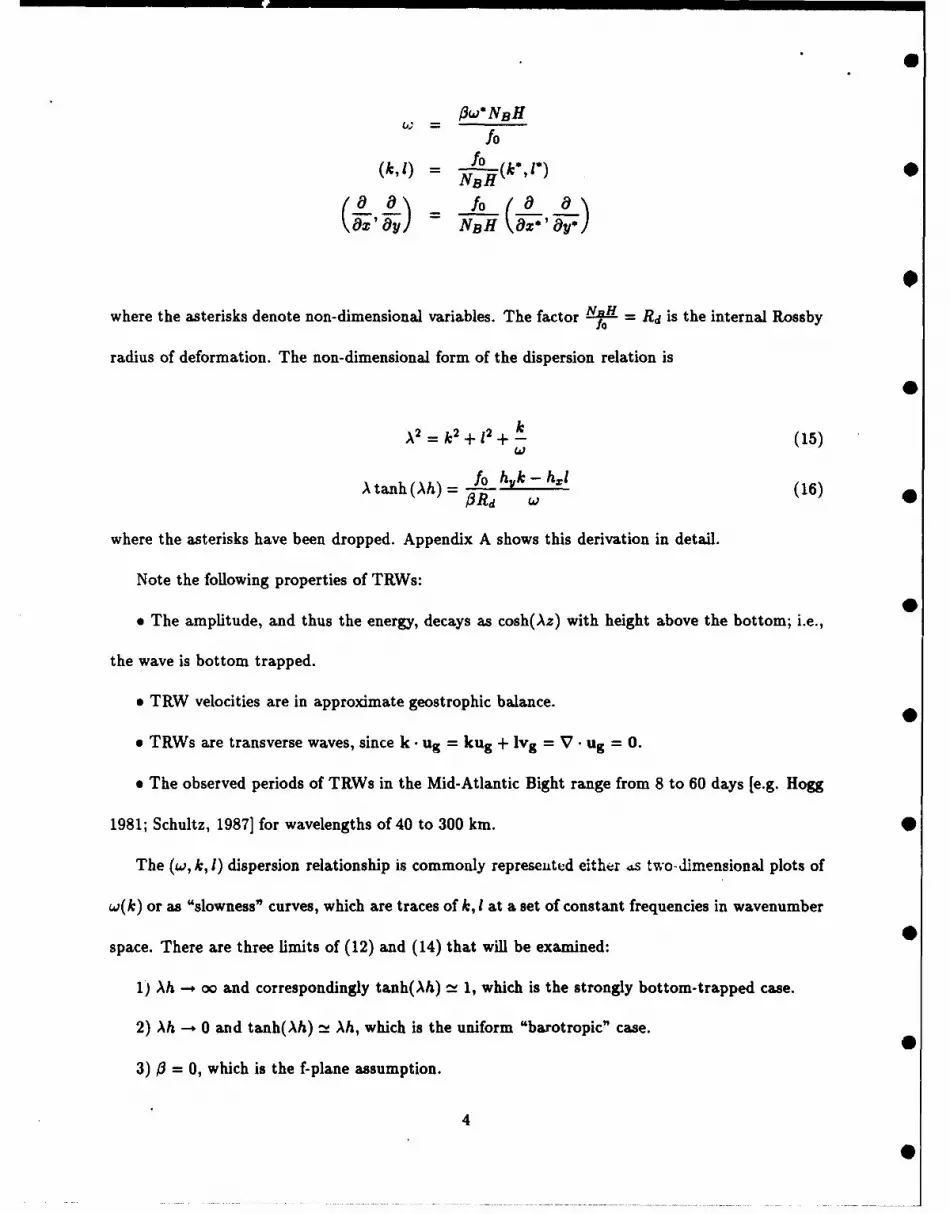
In the second limit, tanh(Ah) -* (h), (14) becomes
I NB2 NA2h = y) (hyk - h.,I)
When this is combined with (12) the result is
(k + E) 2 + (I+ F)2 = G2
where
/3fh 31E=
2w 2wh
F = fhx2wh
G= ( - 2 +h) (fh)2)
This is the equation of a circle. The solution for this barotropic case at site B3, assuming the Test
B3 values, is shown in Figure 3.
7

In the third limit, 0 = 0, (12) becomes
\ 2 (,) 2 (k2 + P2)
which, when combined with (14) does not yield a simple analytic solution. Thus this limit is
solved using numerical techniques together with the Test B3 values. Figure 4 shows the resulting 9
dispersion relation.
In reality, TRWs should fall somewhere between the first two limits. Figure 5 shows a numerical
solution for the dispersion curve using the Test B3 values but without specifying any limits. A
comparison of Figures 2 and 5 reveals that the bottom-trapped case, where tanh(Ah) - 1, is an
excellent approximation for the full solution (at least for waves specified by the Test B3 parameters).
Finally, Figure 6 shows the dependence of the full dispersion relation on frequency. Numerical
solutions for four different wave periods are shown, 24, 32, 40, and 48 days. All four of these
wav,.vectors essentially point either upslope or downslope; the best alignments were found with the
longest period waves. As seen in Figure 6, for wavelengths greater than 75 km (k < .0001), k and
1 vary only slightly for these moderate changes in frequency.
4 Ray Tracing
The following discussion was adapted from LeBlond and Mysak [1978]. There are three steps
involved in ray tracing. First, the equations describing the system are developed. This includes
the expressions for the dispersion relation, the group velocity, the time variation of the frequency,
and the dependence of the frequency on the environmental parameters (such as bottom slope and
water depth). Second, initial values for position, wavelength, and frequency are chosen, and the
corresponding group velocity, c., is computed. Third, the wave packet is progressed with velocity
0c9 for a time 6t, and a new wavelength and frequency are found by integrating the equations from
8J
2.0 xiO 4 - I I X I I
*I
0.0 x100 --J/
-2.0 X C-4/
-4
-4.0 x10- I /
-4.0 xlO- -2.0 x10- 4 0.0 x10 0 2.0 x10⁻⁴
K
Figure 3: The uniform, barotropic dispersion relation for a TRW assuming the Test B3 values.Units are m-.
.J 0.0 xlO0-'
-4.0 x10⁻⁴
-4.0 x10- 4 0.0 x10 0
K
Figure 4: Numerical Solution for the j = 0 dispersion relation in which the Test B3 values weused. Units are m-
9

"2 C "--4
2.C xi,.,
02.:
-2.. x2.
KK
I
-. :-.0 xlO-' -2.0 xlO-4 0.0 xlO° 2.0 xlO- 4"
K
Figure 5: Numerical solution to the full dispersion relation. Units are m- 1.
2. x •C - I I I -4
0.C x'0° -
-,-
-2.C x'0 ,
-4.0I I I I I
-4.0 x10- 4 -2.0 xlO- 4 0.0 x10 0 2.0 X10⁻⁴
K
Figure 6: Numerical solutions for periods 24, 32, 40, and 48 days. The crosses denote a period of24 days, the square is a 32 day period, the triangle denotes the 40 day period, and the diamond isthe 48 day period. Units are in m- 1
10

step 1 over the time interval 6t. The second and third steps are repeated to obtain a path.
To form a mathematical expression for the ray tracing consider a plane wave, with amplitude
A(x, t) and phase S(x, t),
0(x, t) = A(x, t) exp[iS(x, t)] (19)
It is assumed that the amplitude of the wave varies at a much slower rate and over much larger
spatial scales than the phase. The local wavenumber k is defined as
k=VS
and the frequency w as
asOt
Cross-differentiation of these two definitions results in the conservation of wave crests equation
A- + W = 0 (20)
Here k is the directional density of wave crests and w is the flux of wave crests past a fixed point.
By considering both the dynamics of the wave type and the environmental parameters, it is possible
to relate k and w by using the dispersion relation
w(x, t) = a[k(x, t); y(x, t)] (21)
where 7 represents the environmental parameters. If the dispersion relation (21) is substituted into
the conservation of wave crests (20), the result in tensor notation is
Oki +O ca A_ 0
"-i Oki Ozz 87 Oxi8kf
Since the wavenumber is defined as the gradient of the phase, its curl must vanish; thus eiik = 0
and so = •.••. Using this and the definition of the group velocity, ci, = f, the above equation
may be rewritten in vector notation as
dlk Ok Do=. +cg.Vk= -v7 (22)
011

where it a & + c. • V is a derivative moving with the wavepacket. An expression for the variation
of w can be found by differentiating the dispersion relation (21) with respect to time and using the
conservation of wave crests (20) to eliminate k. The result is
Ow Oa Oki 8a 0-y aa aw Ooa-/t0k• 0 Di O'y07 OkOx S078T-t = Fkj at + 8-y 5T Fk: 7x + Ty 0t
Rewriting in vector notation similar to (22) gives the variation in w along a ray path
dw Ow +lac V (23)dt Ot 9-Y ,Ot
Thus the equations which describe the system are
w(x,t) - o[k(x,t);'y(x,t)] (24)
dx _ ea (25)
dk _ aadk Sa (26)dt - 'YV
di• S 07& I; _ 8 f ( 2 7 )dt 0- at
5 Wave Tracing Programs
This section describes the processing steps for ray tracing. The MATLAB code (or FORTRAN,
in the case of the first program GET-ETOPOII.FOR) are given in Appendix C.
5.1 Preparing the Topography
One of the most important features of this method is that real bottom topography is used. In
order to remove all small scale topographic fluctuations that would not affect the waves but will
influence the resulting spline fit, the topography must be gridded and smoothed. Figures showing
the progressive results of this process are presented in Appendix B.
12

5.1.1 The Raw Bathymetry
The raw bathymetry can be obtained from the NCAR ETOP05 earth elevation data set which is
a gridded topography array on a -L a grid. The data set is gridded in equal increments of latitude
and longitude rather than kilometers so the gridding in the x and y directions is slightly different.
Since the area of study will normally encompass only a small fraction of this data, a program called
GETETOPO-II.FOR is used to select just the bathymetry for the area of interest. It is best to
choose the area of interest generously, so that boundary effects of the smoothing filter (discussed
later) will be minimized in the actual study area.
The program GET.ETOPOII.FOR is based on a program GETETOPO.FOR (written by
John Lillibridge at URI). The program has been modified to remove the z-scaling option and to run
on a micro VAX computer. The program is executed by the command file GET-ETOPO.COM,
which must be modified to contain the appropriate input and output file names.
5.1.2 Remove unwanted features
After windowing the bathymetry, it is necessary to remove some isolated features. In this for-
mulation only waves in regions where WKBJ approximations are valid (i.e. where the topography
varies on a much longer scale than the wavelength). Thus features that violate this must be re-
moved or the subsequent smoothing process will spread those features to the region of interset.
For example, bathymetric features that are narrow compared to a wavelength would approximately
generate Taylor-columns to the waves; thus it is better to eliminate these narrow features. The
larger features, such as isolated large-diameter seamounts or chains of seamounts, act as scatterers
and must be removed since reflection is not included in the formulation. The problem features are
removed by reducing their vertical extent. For example, a seamount that was on a slope of average
depth -3500 meters and rose to -2800 meters would cause problems so all grid points in the region
13

of the mount that had a value of greater than -3400 meters would be set equal to -3400 meters,
effectively shortening the seamount.
The MATLAB routine LANDSCAPE.M is used to eliminate unwanted features. A mouse
is required to run the program. The mouse is used to focus in on the feature to be shortened. A
seamnount is selected and eliminated by clicking with the mouse, first on the lower left and then on
the upper right corner of the seamount. At the 'landscape level?' query give the desired depth of
the seamount (e.g. -3500). The program will continue to loop through these steps as long as the
user types 'y' to the 'continue' prompt. The bathymetric contours may be selectively labelled. This
is accomplished by clicking with the mouse on the desired contour at the 'manual' prompt. After
all features have been editted, answer 'n' to the 'continue' query. Save the variable 'mowed-BATH'
to a disk file; this is the new bathymetry data set.
5.1.3 Filtering 0
After removing the unwanted large-scale features, it is necessary to fiter out the small-scale
features that in reality do not affect the waves, but in this formulation would cause considerable
noise in the calculation of the environmental parameters -t and V7 . The TRWs of interest have
wavelengths ranging from about 110 km to 330 km. Therefore a cutoff wavenumber of - was
chosen for the wavenumber filter. MATLAB computes the filter coefficients from the ratio of the 0
cutoff wavenumber to the Nyquist wavenumber.
The program for filtering the topography is a MATLAB routine called FILTER2.M. To run
the program, the user supplies the coefficients for the spatial gridding and the 'mowed-BATH' data
set. The smoothed bathymetry, Y, should be saved in a disk file for later use.
14
5.1.4 Compute spline representation
The final step in preparing the topography is to fit a series of B-splines to the bottom depths. This
is done so that the gradient of the depth, Vh, can be computed for any given location. Because
B-splines are linear processes, the two dimensional grid of bathymetry can be treated one dimension
at a time. The B-splines are first fit to lines of constant latitude. Then another set of B-splines
is fit as a function of latitude (i.e. along lines of constant longitude), creating a two dimensional
B-spline expression for the bathymetry.
The program that fits the B-splines is called COMPUTE-SPLINES3.M. The code is com-
mented heavily. Many of the commands are concerned with reducing "undulations" at the edges
of the domain. These are reduced by augmenting the series to be interpolated. The arguments
of the program are the latitude and longitude of the first point of the filtered bathymetry data
set. It should be noted that the constant 'diat' must be specified prior to executing the program.
This constant specifies the grid spacing of the input array of bathymetry. (For example, for a grid
spacing of half a degree, set dlat = 0.5). The output variables 'c, cprime, c2prime, and xknots'
should be saved in a disk file. (Use an output file name such as SPLINE-110 to indicate what
filter was applied to the input bathymetry data.)
The routine TEST-SPLINES uses the B-splines variables to solve for the depth, bottom slope,
and their gradients at a given location. It is executed in each ray tracing step. In addition to the
B-spline coefficients, the latitude and longitude of the point must be supplied.
5.2 Getting the initial wavenumber
As noted previously in step 2 of the Ray Tracing discussion, it is necessary to obtain initial (k,, 4j)
estimates for the wavenumber vector. These values are needed in order to compute the initial group
velocity of the wave packet. The MATLAB routine INITVAL.M requires the user to supply the
15

position of the starting point of the TRW, •3, fo, NB, H, and Vh, as well as the wavelength and
frequency of the wave. The outputs are k and I as well as the bottom trapping coefficient A and
the propagation angle 8.
Prior to running INITVAL.M, a five element row vector called 'parms' must be created. The
five elements of this vector are 3, dt, fo, H, and NB. The second element, the time step dt, is not
used by this program so it is not crucial to supply its correct value. (However, dt will be used in a
subsequent program.) The third and fourth elements are the Coriolis parameter and the average
water depth from sea surface to sea floor. The final element is NVB, the Brunt-Vaisili frequency.
The routine INITVAL.M also requires the depth, h, at the starting point of the TRW as well
as the bottom slopes h, and h.. To find the value of h, h=, and h. at this position the user must
run the MATLAB program TESTSPLINES.M using the B-spline coefficients obtained from the
COMPUTE-SPLINES$.M program together with latitude and longitude of that point. The
output of the TESTSPLINES.M program should be placed in variable called 'gradh' for use by
the program INITVAL.M to find the wavenumber.
Four additional inputs are required before executing the INITVAL.M program. Set 'omega'
to be the angular frequency, (2), of the TRW in s-I and set 'LAM' to be the wavelength in km.
The longitude and latitude of the starting point are specified as 'x' and 'y.' Once all of the variables
necessary to run INITVAL.M are specified, the program may be executed. The initial k and I
values, as well as the bottom-trapping coefficient A and the propagation angle 9 (measured from
east) of the TRW are calculated by the program.0
5.3 Tracing
, The MATLAB routine called TRWTRACE.M traces the wave path in the manner discussed in
the section entitled Ray Tracing. The routine contains a self check to see if the error is becoming
16

too large. For this test, a new frequency, wi, is computed using the new wavenumbers. This is then
checked against the initial frequency by wcheck = - Ideally the frequency should not vary
over time. However due to computational error the frequency does change and this test warns if the
error is becoming too large. Tests (discussed later) show that for the 40-day period waves, errors
in wcheck of as much as 25% will not significantly alter the important wave parameters, including
the path, wavenumber, group speed, or the bottom-trapping coefficient.
There are several variables that need to be assigned prior to running TRWTRACE.M. First,
the time step increment dt (the second element in the 'parms' array) must be set. This program
allows the wave to be traced forward (positive time increment) or backward (negative time incre-
ment) in time. The time increment is specified in hours. Second, put the longitude and latitude, in
that order, into a 2-element row vector called 'loc' where longitude is measured in degrees east (e.g.
73W is -73). Third another row vector called 'k' should containg the initial ki and 1i values. Finally,
the user must specify the name of the file containing the B-spline variables (e.g. SPLINE_110).
This is an approximate guide to the execution time of the TRWTRACE.M program on a
DEC 3100-76 computer. The major time-consuming step is in the calculation of Vh which requires
the computation of new B-spUne variables for each new position. The execution time for this step
is lengthed greatly if a dense spline set is used. For example, if the B-splines have been fit to a 15
by 25 grid then to run TRWTRACE.M for 50 time steps, the total run time is approximately 15
minutes. Denser filter grids significantly slow down the program; for example using splines fit to a
85 by 145 grid, a 50 time step run would take 1.5 hours.
5.4 Examples
Choosing the ray tracing parameters, such as filter size and time step, can be difficult. One
recommendation is to conduct test runs, specifying different choices for each parameter and compare
17

the results. That way the time efficiency can be weighed against the desired accuracy. The following
examples (Figures 6-10) show the effects of various choices of these parameters on tracing TRW
ray paths, from a detection site in the SYNOP Inlet Array to a potential generation region in the
SYNOP Central Array. (Thus here the time steps will be negative).
For the following cases a consistent set of parameters was used and only one parameter was
varied at a time. Unless stated otherwise, the bathymetry wavenumber filter size was 330 kin, the
time step was eight hours, the period was 40 days, the wavelength was 130 kin, and the launch
site was B3. TRWs of this wavelength and period have been observed in the Inlet Array (Pickart
and Watts, 1990). Several parameters were also specified; /3 = 1.8 x 10⁻¹¹ m-is-1 , f = 9 x 10⁻⁵
s-1, and H = 4000 m. As mentioned earlier, NB was set equal to a constant value, an appropriate
value for the Gulf Stream region being NB = 1 X 10⁻³ s- 1 (Pickart, personal communication).
Figure 7, shows the effect of varying the time step (dt) on the wavepath. Time steps of one
hour and eight hours were tested. The paths for these two runs are almost indistinguishable; the
only difference being that the total wave distance travelled was about 2% shorter for the dt = -1
hr case due to a slower group speed. Figure 8 compares how several of the parameters varied over
time for these two runs. The plots of the total wavenumber (K), the average bottom slope (gradh),
and the bottom trapping coefficient (A) show little difference between the two runs. However, there
is a very large difference in 'wcheck', a measure of the percent variation of the actual frequency
in the run compared to the correct frequency. A value of zero for wcheck indicates no error in
computed frequency. In Figure 8 it is obvious that the frequency errors are high when dt = -8
hours; however this appears to have no effect on the predicted wave path (Figure 6). On the other
hand differences in the actual frequency result in differences in the group speed C. for the two test
cases. Figure 8 shows that when dt = -1 hr the TRW travels about 2 - 3% slower than when
dt = -8 hrs.
18

__I 1 I.I . .I I I I . I ..,,,.I,
40.0 --- ----
38.0 -," '", "
36.0 -
I I I
340.0I - -•
T-I I I
I -
I ,
i S I /
34.0 ' ~I "' 'I' I -67.0 I"
-77.0 -75.0 -73.0 -71.0 -69.0 -67.0 -65.0
Figure 7: B3 launch with dt=-1 hrs and dt=-8 hrs for 410 time steps and 52 time steps, respec-tively. Approximate run times 1.5 hours and 15 minutes, respectively. The cross denotes the eighthour time step and the square is the one hour time step run. The dashed lines are t.he 330 kmfiltered bathymetry.
19

0.20 -
0.00
2.20z
1 80-
Y 1. 0 LI
3).22F
0.067
2.00-
1.20
0.80 -
55.0
U 45.0
35.00. 200. 400.
Hours
Figure 8: Comparison of dt=-1 hrs and dt=-8 hrs. The cross denotes the eight hour time steprun and the squares are the one hour run.0
20

The effects of varying the degree of smoothing of the bathymetry were also tested. For example,
for the area between the SYNOP Inlet and Central Arrays, the 110 km filter gives a more realistic
bottom topography than the 330 km filter (see Appendix B). However, in order to fit B-splines to
the 110 km filtered bathymetry without aliasing, the filtered data can only be subsampled every
6 degree. This leads to a very dense rpline set and considerably slows down the tracing program.
Using a 330 km filter for the bathymetry permits subsampling at every ½ degree without aliasing,
and in turn leads to a sparser spline set and a shorter run time. Figure 9 shows the predicted wave
paths from site B3 for three different filter sizes, 110, 220, and 330 km. Despite the differences in
in the smoothed bathymetries the end positions of the predicted wave paths are quite close.
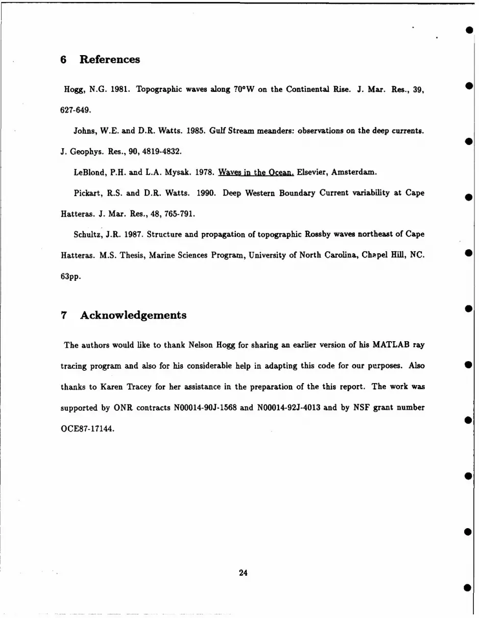
The influence of the choice of launch position and wave period was also tested. Figure 10 shows
launches from sites B2, B3, and B4 of the Inlet Array, which are about 50 km from each other. All
other parameters have been held constant. The three paths appear to parallel one another. The
biggest difference between them is the total distance traveled, impling that the group speeds are
different. The slowest speeds were obtained for the wave traced from site B4, where IVhI is the
smallest.
The predicted wave path also depends on the wave periodicity. Figure 11 shows the traces of
three waves launched from site B3 with periods of 32, 40, and 48 days. In this case the waves travel
approximately the same distance (There is '..tle variation in longitude of the end points). On the
other hand there is a difference about 20 latitude between the trace endpoints for waves with the
32 day periodicity and the 48 day period waves.
These results can be summarized as follows. Firstly, an accuracy of 10 kilometers in the 'launch'
site of the wave gi res consistent path predictions. Additionally, a 10% error in wave period will
also give consistent path predictions. Second, more accurate topography is obtained when a 110
km wavenumber filter is applied. Finally, a time step of dt = -8 hours is adequate for most cams;
21
40.0
38.0
36.0
34.0 - I I I t I I t I I
-77.0 -75.0 -73.0 -71.0 -69.0 -67.0 -65.0II
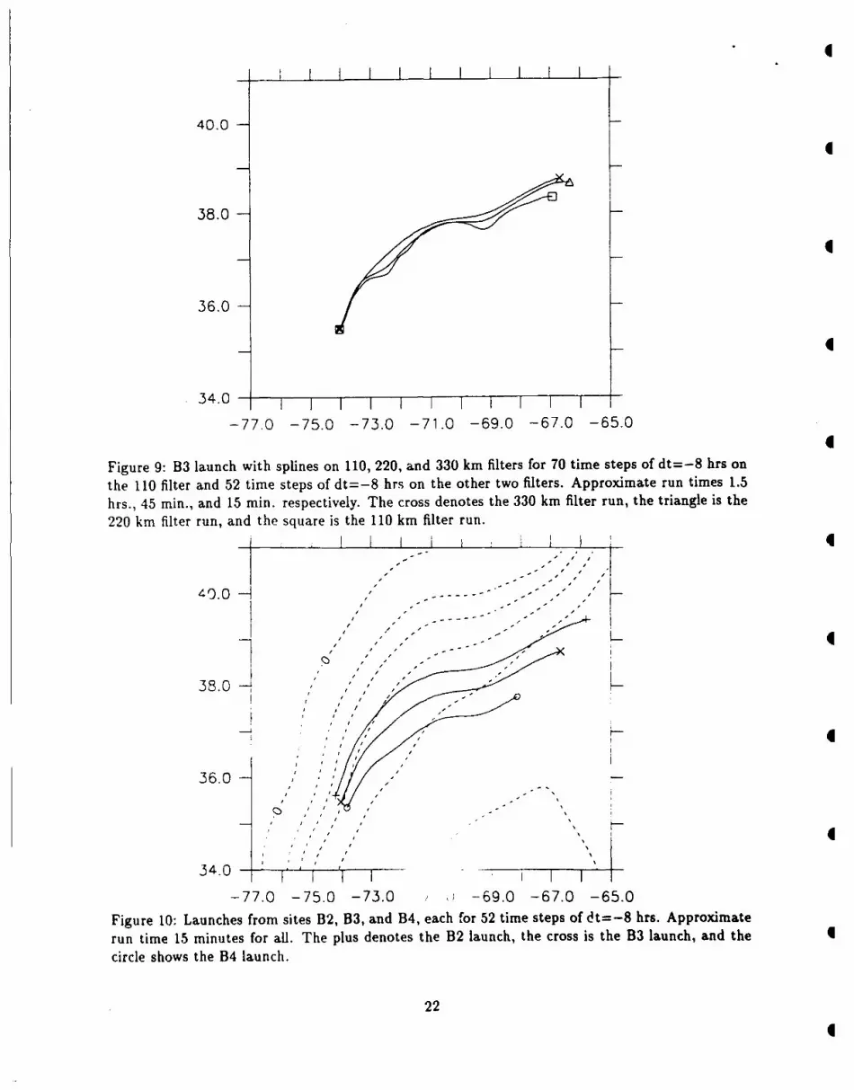
Figure 9: B3 launch with splines on 110, 220, and 330 km filters for 70 time steps of dt=-8 hrs on
the 110 filter and 52 time steps of dt=-8 hrs on the other two filters. Approximate run times 1.5
hrs., 45 min., and 15 min. respectively. The cross denotes the 330 km filter run, the triangle is the
220 km filter run, and the square is the 110 km filter run.
I I •
4-9.0 -- ---- - ,
L.38.0 ' , , - - - ..,-
I ' 'I
36.0, , '
-77.0 -75.0 -73.0 -69.0 -67.0 -65.0
Figure 10: Launches from sites B2, B3, and B4, each for 52 time steps of dt=-8 hrs. Approximaterun time 15 minutes for all. The plus denotes the B2 launch, the cross is the B3 launch, and thecircle shows the B4 launch.
22
j i I

I II I I I I I !
40.0 - -
* I I°
38.0 , , ,
III / €"
* II
36.0 - , '""
34.0I -i T
-77.0 -75.0 -73.0 -71.0 -69.0 -67.0 -65.0
Figure 11: B3 launch with different periods, each for 52 time steps of dt=-8 hrs. The plus denotesthe 32 day period, the cross is the 40 day period, and the circle shows the 48 day period.
using dt -1 hour is only necessary when extreme accuracy in group speed, c.., is needed.
23
0 Ii•\
6 References
Hogg, N.G. 1981. Topographic waves along 70OW on the Continental Rise. J. Mar. Res., 39,
627-649.
Johns, W.E. and D.R. Watts. 1985. Gulf Stream meanders: observations on the deep currents.
J. Geophys. Res., 90, 4819-4832.
LeBlond, P.H. and L.A. Mysak. 1978. Waves in the Ocean. Elsevier, Amsterdam.
Pickart, R.S. and D.R. Watts. 1990. Deep Western Boundary Current variability at Cape
Hatteras. J. Mar. Res., 48, 765-791.
Schultz, J.R. 1987. Structure and propagation of topographic Rossby waves northeast of Cape
Hatteras. M.S. Thesis, Marine Sciences Program, University of North Carolina, Chapel Hill, NC.
63pp.
7 Acknowledgements
The authors would like to thank Nelson Hogg for sharing an earlier version of his MATLAB ray
tracing program and also for his considerable help in adapting this code for our purposes. Also
thanks to Karen Tracey for her assistance in the preparation of the this report. The work was
supported by ONR contracts N00014-90J-1568 and N00014-92J-4013 and by NSF grant number
0CE87-17144.
24

8 Appendix A The Dispersion relation derivation01
This is the derivation of the dispersion relation (equations (15) and (16)) that was shown in the
Dynamics and Kinematics of TRWs section. Begin by using the same five equations, the two
linearized horizontal motion equations, the incompressibility equation, the hydrostatic equation,
and the linearized density equation, which are repeated here.
- f,= 1OP (28)
Ft 1O ax/DV 1+fu= 1a (29)
i POa ay*U + + w = 0 (30)Fx +DY -Dz
1- P'g = 0 (31)
Op' I poN 2w = 0 (32)t g(
Now, taking the time derivative of (31) and substituting (32) into it yields
t 5- +poN2 w= (33)
Next, take • of (29) and subtract 4 of (28) to give
D' v a% =0=a_axot 19Y& ax f O #
Substituting (30) for the quantity in paranthesis and moving it over to the right hand side gives
•a fa O uV 8 WSF -- + OV= f (34)
which is the linear vorticity equation. Let the quantity in paranthesis be denoted as C. Now, by
* using the leading order geostrophic balance it is possible to get relations for v., u., and (e
V" = O/Po (35)
* 25

ug = Lop' (36)
1= j--v2p! (37)
Here V = +-- . Substituting these into the linear vorticity (34) gives us the Quasi-Geostrophic
Vorticity (QGV) Equation
1[0 a p1 OWf- [ (V p ) + /3 -#T, o - ( 8To P0 & OZ(38)
Now take . of (33) to get 0
which is substituted into the right hand side of the QGV (38) to give
1 ~ ~ ~ ~ 8 [±Vp)#P=f± ( 1 OP')7. [o , + Ox &. ]z poN2 OZ
Multiplying both sides by Po and combining the time derivatives gives
_2p, + ±[ 2,p•1_ a() oP
Tt Oz N D5z]+ #ox=
Using Hogg's (19811 technique approximate the varying N with a constant Brunt-Vaisili frequency,
NB, at the bottom to obtain a workable equation of one variable.
0[ )282l + #Lp =5t_[~j + _L -ýZ-2(39)
This is the same expression as equation (6). Now for the top boundary condition at z = 0 the rigid
lid approximation is used to force w = 0. So (33) simplifies to
82p,
Wz' . 0 (40)
Assuming no normal flow at the bottom, where w = u. -Vh
1 [Op Oh Oip'Oh]
26
Substituting into (33) gives02p' N2 OP Oh Op'Oh(
*Oz = fo [ axy a]y (41)
where z = -h(x, y). A plane wave solution of the form
* = A(z) exp[i(kz + ly - wt)] (42)
is sought. Substituting (42) into (39) gives
( o y2 2A I -/kplS12+ f z
0 LPf(_k2 - k+NB 5Z2;
From this point, the prime will be dropped from pressure p, and the subscripts will be dropped
from f and N. Taking the time derivative yields
iwp(k2 + 12 _ --)21 &A\N / ) +'Oikp = 0
Divide by both i and p, since they are non-zero, leaving
W•(k2 +[. 12 2 02A- .• -• ) + ,Ik :0\N A z 2
Dividing by w and regrouping gives
- 1-2A + (k2 + +12+ =0
Multiplying by -(NY)2A produces
02--A -A (k2 + 12 +-) =0
If the quantity inside the square brackets is defined as A2 the result is
02 A-z2 A = 0 (43)
where
= (k2 + 12 + -)(44)
27

Using (44) and the top boundary condition (40) it is possible to solve for A(z)
A(z) = cosh(A\z) (45)
Putting this into (42) and then substituting into the bottom boundary condition (41) the left side
of (41) becomes
a-P = -A sinh(-,\h)iw exp[i(kz + ly - wt)]
and the right side of (41) becomes
N2 /8heOp Dh9p N2. / h 8 h t7 A Op Oh = -N-2icosh(-Ah)exp[i(kx+ly-wt)] (Lk- I)
Setting the two sides equal and cancelling the common i and exp[i(kx + ly - wt)]
N 2
-A sinh(-,\h)w =N cosh(-A\h)(hk - hIl)
where the derivatives of h are denoted as h. and h.. Dividing through by cosh(-A\h) gives
N 2
-A tanh(-Ah) -(hyk - hal)
Since tanh(-z) = - tanh(x), this can be written as
N 2
A tanh(Ah) = N-2(hyk - h.l) (46)Wf
At this point, the equations are easier to work with if they are non-dimensionalized. Specify the
following factors
h = Hh*
O-H
wO --
(k,1) - NH
28

0
ax 69 - NH (8xL~*')
Where the asterisks denote non-dimensional variables. Substituting these into (44) gives the
non-dimensional form
A'*2 =(N'\ 2 (ka 2je2 + 12f2 + 3k'! 2
H.2 f N2H2 +-2 N 2 H2-- /3
This expression can be simplified by multiplying by H 2, moving - inside the parenthesis, and
cancelling the 3-terms to obtain
•A.2 = k*2 + 12 + (47)
The non-dimensional form of (46) is
A A* N2 f Hf If. kl'f h * 1-fSH-tanh(HHh*) = f7IoNHNH O*N (h f f NN)
Cancelling the common factors gives
f2 (h,k" - h'l')* A* tanh(A*h-) = f-HN *
Finally, introducing the radius of deformation, Rd = • yields
A-=f (hk- hl*) (48)
Equations (47) and (48) together comprise the non-dimensional dispersion relation for this system.
* 29

9 Appendix B Example Bottom Topography Preparation.
Following are three figures that show the progression of a region of bottom topography as it is
prepared for ray tracing. The area shown is 65-77 W and 34-41 N.
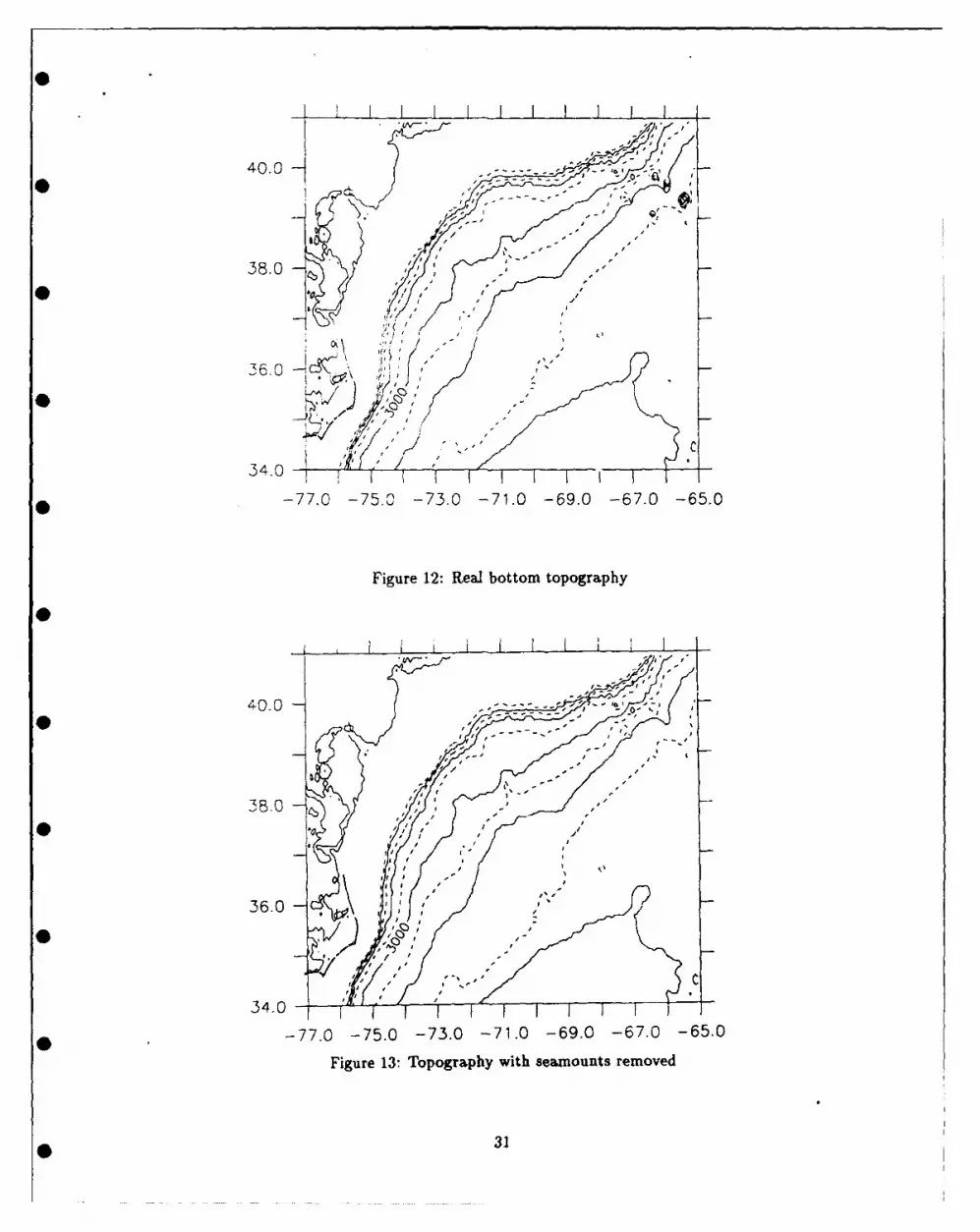
The first is the original bottom topography, as taken from the ETOPO5 data set. Figure 12 still 0
has the sea mounts and all of the true topography shown. After the LANDSCAPE.M program
is run the seamounts that were in the upper right corner are no longer there, creating a topography
such as in Figure 13. Afte *e filtering has been done the result is Figure 14. Here a 110 km
filter has been used. Figure 15 shows the 220 km filtered topography. Figure 16 shows the 330 km
filtered topography.
0
30
40.0
38.0
356. 0 K-J3 K/
34.0 *
-77.0 -75.C) -73.0 -71.0 -69.0 -67.0 -65.0
Figure 12: Real bottom topography
40.0)
30
360
-77.0 -75.0 -73.0 -71.0 -69.0 -67.0 -65.0
Figure 13: Topography with seamounts removed
31

I I I I I
40 .0 -- ,- --
38.0 -
36.0 /
34.0
-77.0 -75.0 -73.0 -71.0 -69.0 -67.0 -65.0
Figure 14: 110 km filtered topography. Note the coastline gets smoothed also and appears as the0 contour.
I I I I I I I
40.0
38.0 -
36.0
38.0
,_ I I
I •
34.0- -
-77.0 -75.0 -73.0 -71.0 -69.0 -67.0 -65.0
Figure 15: 220 km filtered topography.
32

S s
40.0
38.0
, / I
I I
34.0 -
-77.0 -75.0 -73.0 -71.0 -69.0 -67.0 -65.0
Figure 16: 330 km filtered topography.
330 33
10 Appendix C Program Codes
Most of the following program code is written in MATLAB. A good reference for MATLAB
is Pro-MatlabTM for VAX/VMS Computers, 1991 by MathWorks Inc. The lone exception, the
program GETETOPOII.FOR is written in FORTRAN. 0
34

Ae e
425
0 o'q '-4cqC904 -0 -j - "
en0
Is~ ~ C0 eq-
co& 4545 00 0f10 lv
-~~ aul 4 E 5 41 4jC'-4 CO CO 5415~ &E.44 a l 4jil4 48,040I V0 ' . ~ ~ ~ 4~g e
en ~ I I ~ JSI 555 55 q,0 45 0-4E Id 8 - 1
44 ~ -0- ) A
-,4 U) A~aa -4
01 91QUO~~4 Op 0OiOUC 4C O O0-000
Vq 4.1 05 ý4 4 45
01f 9ý 01 U .- 4
0 . j 0~ 0 1
E 4)-- j
-4~~~~~ 4)44 . 44 -
C6 a 0
4-1) 4101~~~ 0- 1uuuuuuuuuduut~~~~~~~ u 5 - uuau0u 0 suu0 u~ u 45 uauu
01 *54~~* 4eq,35

-4
4.
-4-n
41 U
* 4 .'
41V4
.fl
Up py pi u p
36

0 -
00
-14
1411
* f4
-4 aa a 10
414 1 isF
Ai -4
go dipa... 4 ~ - *37

___ I
6
I
0
0
6
-4
-4 6
0%0%
I
(.4
'.4 6zg,� � 8
.1 �11111112 !�liii.
038

0m
-44
-4j
.14 .01
'.1
'.04
M 0M.A4
04 C)'iA4
04 01
do O a 00 aw a a d 0O-0 0 .
.. . . .. .. . .. .... . ..
%4S
4w4-
4 1 -441:4
0%0
Id oS0% 0 P.td 2 ld pd
S 44, 0i
I~ I
4~40

0~~~~~~~~~~~~~ q_________________________
044 ;
04 04 4-
3i :4
'-4a 41
-41 -
*4 *0.
41:
-~ i .j ~ ;41

, + 0. :1 -Cl• .. + :lJ + 14 M' , jbc . 1
4-4r . -4 a4
0% 96 0%cic
)t C4- 0 -" -
-4 C &-40r 4 4ý
'Z + :z+ +;.+ .- , ++•,+, ,,.,,: ..., .:,,+,,,.+,•- , .11 :, :... ,r .: ýZý.CIO,+ i o : 4:": fii".4' -" - .• ."
0. 0
,,4 + 4 0" -s.-." + -
E -- M C-4 CA- 4-1 +4. 4C
CIO M - -I C1 4 a
ci is+ + v if -a I--C
S -,'..I.',, U
.R ~~4- 14j~ 4 '0
%.4z- fC.
t: 'I+ Bl +
. . . . . . . .. .. .
,- A ' I .
C' I 1!0% +: I+4'V 0 -4 ++•"•. - •.
+ •, -. '+.4+ *01-0 i - :-".. '--Cq•++ +. 0'" "--"C-C.
0 4A'
~. 0.0
41 8 - CA
Is. 8m. . . .fCCI
I--~141
42

0a
0m
a04
-44
0to
-43

SECURITY CLASSIFiCATION OF T15 PAGE
REPORT DOCUMENTATION PAGEIa. REPORT SECURITY CL.ASSiFICA•ION Rb RESTRICTIVE MARKINGS
I~n__l me a ,i f'i,-A
Za. SECURITY CLASSIFICATION AUTHORITY 3 OISTRIBUIiON/AVAILABILITY OF REPORTDistribution for Public Release;
Zb. DECLASS;FICATION/ DOWNGRADING SCHEDULE Distribution is unlimited
4. PERFORMING ORGANIZATION REPORT NUMBER(S) GSO 5. MONITORING ORGANIZATION REPORT NUMBER(S)niversity of Rhode Island Tech Report 93-1
Graduate School of Ozeanography
6a. NAME OF PERFORMING ORGANIZATION 6 6b. OFFICE SYMBOL 7a. NAME OF MONITORING ORGANIZATIONUniv. of Rhode Island (If applicabJle)
Grad. School of Oceanography I
6c. ADDRESS (City, State, and ZIPCode) 7b. ADDRESS (City, State, and ZIP Cod*)3outh Ferry Roadgarragansett, RI 02882
Ba. NAME OF FUNDING/ SPONSORING 8b. OFFICE SYMBOL 9. PROCUREMENT INSTRUMENT IDENTIFICATION NUMBERffq'f al Research (Of appliable)
.Natin l Science Fn indntinnI8c. ADDRESS (City, State, and ZIP Code) 10. SOURCE OF FUNDING NUMBERS
800 N. Quincy St., Arlington, VA 22217 PROGRA" PROJECT TASK IWORK UNITc'0ELEMEN' 0. NO. NO. ACCESSION NO.
800 G. St., N.W., Washington DC 20550
11. TITLE (Include Security Classification)
Ray Tracing on Topographic Rossby Waves.
12. PERSONAL AUTHOR(S)
Christopher Meinen. Erik Fields. Robert Pickart. D_ Randolph Watts13a. TYPE OF REPORT 13b. TIME COVERED 14. DATE OF REPORT (Year, Montrh, DOay) 5. PAGE COUNTSummary FROM TO I May, 199316. SUPPLEMENTARY NOTATION
17. COSATI CODES 18. SUBJECT TERMS (Continue on reverse if necessary and identify by block number)
FIELD -GROUP SUB-GROUP Topographic Rossby Waves, SYNOP, and Mid Atlantic Bight
19. ABSTRACT (Continue on reverse if necessary and identify by block number)Topographic Rossby Waves (TRWs) have been identified with the largest variability
in deep current meter records along the continental slope in the Mid-Atlantic Bight (MAB).Ray tracing theory is applied to TRWs using the real bottom topography of the MAB andthe observed stratification. The depression relation for TRWs is derived and variouswavenumber limits are discussed. A computational method for tracing the waves is presentedincluding the necessity of smoothing the bathymetry. In the examples shown, TRWs withperiods of 24-48 days generally propagate southwestward, changing their wavelengths from400 to 100 kilometers in responce to the change in bottom slope. TRW paths are shownthat connect from the SYNOP Central Array near 68*W to the SYNOP Inlet Array near CapeHatteras.
20. :ISTRIBUTION/AVAILABILITY OF ABSTRACT 21. ABSTRACT SECURITY CLASSIFICATION
S UNCLASSIFIED/UNLIMITED 0 SAME AS .RPT r DT'C USERS
22a. NAME OF IESPONSIBLE NOIVIOUAL 22b tELEPHONE (Include Area Code.) 22c. OFFICE SYMBOL
00 FORM 1473, 84 MAR 33 APR ecition may De usea until exnausTea. SECURITY CLLSSiFICAriON OF "H5 '-G.All otier editions are oosolete.