Lecture Notes in Electrical Engineering 281

Koen LangendoenWen HuFederico FerrariMarco ZimmerlingLuca Mottola Editors

Real-World Wireless Sensor NetworksProceedings of the 5th International Workshop, REALWSN 2013, Como (Italy), September 19–20, 2013

Lecture Notes in Electrical Engineering

Volume 281

Board of Series Editors

Leopoldo Angrisani, Napoli, ItalyMarco Arteaga, Coyoacán, MéxicoSamarjit Chakraborty, München, GermanyJiming Chen, Hangzhou, P.R. ChinaTan Kay Chen, Singapore, SingaporeRüdiger Dillmann, Karlsruhe, GermanyGianluigi Ferrari, Parma, ItalyManuel Ferre, Madrid, SpainSandra Hirche, München, GermanyFaryar Jabbari, Irvine, USAJanusz Kacprzyk, Warsaw, PolandAlaa Khamis, New Cairo City, EgyptTorsten Kroeger, Stanford, USATan Cher Ming, Singapore, SingaporeWolfgang Minker, Ulm, GermanyPradeep Misra, Dayton, USASebastian Möller, Berlin, GermanySubhas Mukhopadyay, Palmerston, New ZealandCun-Zheng Ning, Tempe, USAToyoaki Nishida, Sakyo-ku, JapanFederica Pascucci, Roma, ItalyTariq Samad, Minneapolis, USAGan Woon Seng, Nanyang Avenue, SingaporeGermano Veiga, Porto, PortugalJunjie James Zhang, Charlotte, USA

For further volumes:http://www.springer.com/series/7818

About this Series

‘‘Lecture Notes in Electrical Engineering (LNEE)’’ is a book series which reportsthe latest research and developments in Electrical Engineering, namely:

• Communication, Networks, and Information Theory• Computer Engineering• Signal, Image, Speech and Information Processing• Circuits and Systems• Bioengineering

LNEE publishes authored monographs and contributed volumes which presentcutting edge research information as well as new perspectives on classical fields,while maintaining Springer’s high standards of academic excellence. Also con-sidered for publication are lecture materials, proceedings, and other relatedmaterials of exceptionally high quality and interest. The subject matter should beoriginal and timely, reporting the latest research and developments in all areas ofelectrical engineering.

The audience for the books in LNEE consists of advanced level students,researchers, and industry professionals working at the forefront of their fields.Much like Springer’s other Lecture Notes series, LNEE will be distributed throughSpringer’s print and electronic publishing channels.

Koen Langendoen • Wen HuFederico Ferrari • Marco ZimmerlingLuca MottolaEditors

Real-World WirelessSensor Networks

Proceedings of the 5th InternationalWorkshop, REALWSN 2013, Como (Italy),September 19–20, 2013

123

EditorsKoen LangendoenDelft University of TechnologyDelftThe Netherlands

Wen HuCSIRO ICT CentreQueensland Centre for Advanced

TechnologiesPullenvaleAustralia

Federico FerrariMarco ZimmerlingComputer Engineering and Networks

LaboratoryETH ZurichZurichSwitzerland

Luca MottolaDipartimento di Elettronica, Informazione

e BioingegneriaPolitecnico di MilanoMilanItaly

ISSN 1876-1100 ISSN 1876-1119 (electronic)ISBN 978-3-319-03070-8 ISBN 978-3-319-03071-5 (eBook)DOI 10.1007/978-3-319-03071-5Springer Cham Heidelberg New York Dordrecht London

Library of Congress Control Number: 2013954846

� Springer International Publishing Switzerland 2014This work is subject to copyright. All rights are reserved by the Publisher, whether the whole or part ofthe material is concerned, specifically the rights of translation, reprinting, reuse of illustrations,recitation, broadcasting, reproduction on microfilms or in any other physical way, and transmission orinformation storage and retrieval, electronic adaptation, computer software, or by similar or dissimilarmethodology now known or hereafter developed. Exempted from this legal reservation are briefexcerpts in connection with reviews or scholarly analysis or material supplied specifically for thepurpose of being entered and executed on a computer system, for exclusive use by the purchaser of thework. Duplication of this publication or parts thereof is permitted only under the provisions ofthe Copyright Law of the Publisher’s location, in its current version, and permission for use mustalways be obtained from Springer. Permissions for use may be obtained through RightsLink at theCopyright Clearance Center. Violations are liable to prosecution under the respective Copyright Law.The use of general descriptive names, registered names, trademarks, service marks, etc. in thispublication does not imply, even in the absence of a specific statement, that such names are exemptfrom the relevant protective laws and regulations and therefore free for general use.While the advice and information in this book are believed to be true and accurate at the date ofpublication, neither the authors nor the editors nor the publisher can accept any legal responsibility forany errors or omissions that may be made. The publisher makes no warranty, express or implied, withrespect to the material contained herein.

Printed on acid-free paper

Springer is part of Springer Science+Business Media (www.springer.com)

Preface

It is our great pleasure to welcome you to REALWSN 2013, the 5th Workshop onReal-World Wireless Sensor Networks, with a focus of bringing togetherresearchers and practitioners to discuss state-of-the-art and best practices in sensornetworks.

This year we received 32 submissions, originating from over 18 differentcountries around the globe. Apart from a few submissions violating the double-blind requirement, all papers received at least three reviews and engaged in anonline discussion phase. Finally, 10 full papers and 6 short papers were selectedfor this year’s program. As the sensor network field is maturing the programincludes a wide variety of topics, ranging from RF front ends and directionalantennas, via MAC protocols and routing, to applications studies and real-worlddeployments. In addition to the technical program, the workshop features a posterand demo session with nine entries, making for an exciting event all-in-all.

We thank the members of the technical program committee, the poster anddemo chairs (Thiemo Voigt and Silvia Santini), the publication chairs (FedericoFerrari and Marco Zimmerling), and the local organizers (Mikhail Afanasov andAlessandro Sivieri) for their contributions to the organization of the workshop.Above all, we would like to thank Luca Mottola, the general chair, for keeping uson track and making REALWSN 2013 a reality.

September 2013 Wen HuKoen Langendoen

v

Organization

REALWSN 2013 was organized by Politecnico di Milano, Dipartimento diElettronica, Informazione, e Bioingegneria.

General Chair

Luca Mottola Politecnico di Milano, Italy and SICS Swedish ICT,Sweden

Program Co-Chairs

Wen Hu CSIRO, AustraliaKoen Langendoen TU Delft, The Netherlands

Poster and Demo Chairs

Silvia Santini TU Darmstadt, GermanyThiemo Voigt Uppsala University and SICS Swedish ICT, Sweden

Program Committee

Nirupama Bulusu Portland State University, USAPer Gunningberg Uppsala University, SwedenChamath

KeppitiyagamaUniversity of Colombo, Sri Lanka

Gian Pietro Picco University of Trento, ItalyUtz Roedig Lancaster University, UKChristian Rohner Uppsala University, SwedenKay Römer TU Graz, AustriaJochen Schiller FU Berlin, GermanyCormac Sreenan University College Cork, IrelandTim Wark CSIRO, Australia

vii

Neal Patwari University of Utah, USAOmprakash Gnawali University of Houston, USAYu (Jason) Gu Singapore University of Technology and DesignOlga Saukh ETH Zurich, SwitzerlandNiki Trigoni University of Oxford, UKMarco Zúñiga TU Delft, The NetherlandsPrasant Misra SICS Swedish ICT, SwedenChiara Petrioli University of Rome ‘La Sapienza’, ItalyPhilipp Sommer CSIRO, AustraliaGianluca Dini University of Pisa, ItalyWang Jiliang Hong Kong University of Science and TechnologyGeoffrey Challen University at Buffalo, USAMarcus Chang Johns Hopkins University, USA

Publication Chairs

Federico Ferrari ETH Zurich, SwitzerlandMarco Zimmerling ETH Zurich, Switzerland

Publicity Chair

Mikhail Afanasov Politecnico di Milano, Italy

Web Chair

Alessandro Sivieri Politecnico di Milano, Italy

viii Organization

Contents

Part I Applications

Snowcloud: A Complete Data Gathering Systemfor Snow Hydrology Research . . . . . . . . . . . . . . . . . . . . . . . . . . . . . . 3Christian Skalka and Jeffrey Frolik

The Big Night Out: Experiences from Tracking Flying Foxeswith Delay-Tolerant Wireless Networking . . . . . . . . . . . . . . . . . . . . . 15Philipp Sommer, Branislav Kusy, Adam McKeown and Raja Jurdak

On Rendezvous in Mobile Sensing Networks . . . . . . . . . . . . . . . . . . . 29Olga Saukh, David Hasenfratz, Christoph Walser and Lothar Thiele

Real-Life Deployment of Bluetooth Scatternets for WirelessSensor Networks . . . . . . . . . . . . . . . . . . . . . . . . . . . . . . . . . . . . . . . . 43Michael Methfessel, Stefan Lange, Rolf Kraemer, Mario Zessack,Peter Kollermann and Steffen Peter

Part II Poster and Demo Abstracts

Poster Abstract: Velux-Lab—Monitoring a Nearly ZeroEnergy Building . . . . . . . . . . . . . . . . . . . . . . . . . . . . . . . . . . . . . . . . 55Alessandro Sivieri

Poster Abstract: Visualization and Monitoring Toolfor Sensor Devices . . . . . . . . . . . . . . . . . . . . . . . . . . . . . . . . . . . . . . . 61Lubomir Mraz and Milan Simek

ix

Demo Abstract: MakeSense—Managing ReproducibleWSNs Experiments . . . . . . . . . . . . . . . . . . . . . . . . . . . . . . . . . . . . . . 65Rémy Léone, Jérémie Leguay, Paolo Medagliani and Claude Chaudet

Demo Abstract: Cross Layer Design for Low Power, Low Delay,High Reliability Radio Duty-Cycled Multi-hop WSNs . . . . . . . . . . . . . 73Eoin O’Connell and Brendan O’Flynn

Poster Abstract: Outdoors Range Measurements with ZolertiaZ1 Motes and Contiki . . . . . . . . . . . . . . . . . . . . . . . . . . . . . . . . . . . . 79Marie-Paule Uwase, Nguyen Thanh Long, Jacques Tiberghien,Kris Steenhaut and Jean-Michel Dricot

Poster Abstract: iBAST—Instantaneous Bridge AssessmentBased on Sensor Network Technology . . . . . . . . . . . . . . . . . . . . . . . . 85Richard Mietz, Carsten Buschmann, Dennis Boldt,Kay Römer and Stefan Fischer

Demo Abstract: SmartSync; When Toys Meet WirelessSensor Networks . . . . . . . . . . . . . . . . . . . . . . . . . . . . . . . . . . . . . . . . 91Fiona Edwards-Murphy, Michele Magno, Aidan Frost, Amy Long,Naomi Corbett and Emanuel Popovici

Poster Abstract: Link Quality Estimation—A Case Studyfor On-line Supervised Learning in Wireless Sensor Networks . . . . . . 97Eduardo Feo-Flushing, Michal Kudelski, Jawad Nagi,Luca M. Gambardella and Gianni A. Di Caro

Poster Abstract: An Experimental Study of Attackson the Availability of Glossy . . . . . . . . . . . . . . . . . . . . . . . . . . . . . . . 103Kasun Hewage and Thiemo Voigt

Part III Low-level Components

Node Identification Using Clock Skew . . . . . . . . . . . . . . . . . . . . . . . . 111Ibrahim Ethem Bagci and Utz Roedig

MagoNode: Advantages of RF Front-ends in WirelessSensor Networks . . . . . . . . . . . . . . . . . . . . . . . . . . . . . . . . . . . . . . . . 125Mario Paoli, Antonio Lo Russo, Ugo Maria Colesantiand Andrea Vitaletti

x Contents

MIMOSA, a Highly Sensitive and Accurate Power MeasurementTechnique for Low-Power Systems . . . . . . . . . . . . . . . . . . . . . . . . . . 139Markus Buschhoff, Christian Günter and Olaf Spinczyk

A Remotely Programmable Modular Testbed for BackscatterSensor Network Research . . . . . . . . . . . . . . . . . . . . . . . . . . . . . . . . . 153Eleftherios Kampianakis, John Kimionis, Konstantinos Tountasand Aggelos Bletsas

Part IV Networking

A Scalable Redundant TDMA Protocol for High-DensityWSNs Inside an Aircraft . . . . . . . . . . . . . . . . . . . . . . . . . . . . . . . . . . 165Johannes Blanckenstein, Javier Garcia-Jimenez,Jirka Klaue and Holger Karl

Do We Really Need a Priori Link Quality Estimation? . . . . . . . . . . . . 179Vasilis Vasilopoulos, Daniele Puccinelli and Marco Zúñiga

Redundant Border Routers for Mission-Critical6LoWPAN Networks . . . . . . . . . . . . . . . . . . . . . . . . . . . . . . . . . . . . . 195Laurent Deru, Sébastien Dawans, Mathieu Ocaña,Bruno Quoitin and Olivier Bonaventure

Using Directional Transmissions and Receptions to ReduceContention in Wireless Sensor Networks . . . . . . . . . . . . . . . . . . . . . . 205Ambuj Varshney, Thiemo Voigt and Luca Mottola

Part V Energy

Energy Parameter Estimation in Solar Powered WirelessSensor Networks . . . . . . . . . . . . . . . . . . . . . . . . . . . . . . . . . . . . . . . . 217Mustafa Mousa and Christian Claudel

Experiences with Sensors for Energy Efficiencyin Commercial Buildings . . . . . . . . . . . . . . . . . . . . . . . . . . . . . . . . . . 231Branislav Kusy, Rajib Rana, Phil Valencia, Raja Jurdak and Josh Wall

Contents xi

Wireless Sensor Networks for Building Monitoring DeploymentChallenges, Tools and Experience . . . . . . . . . . . . . . . . . . . . . . . . . . . 245Alan McGibney, Suzanne Lesecq, Claire Guyon-Gardeux,Safietou R. Thior, Davide Pusceddu, Laurent-Frederic Ducreux,François Pacull and Dirk Pesch

Long Term WSN Monitoring for Energy Efficiencyin EU Cultural Heritage Buildings . . . . . . . . . . . . . . . . . . . . . . . . . . . 253Femi Aderohunmu, Domenico Balsamo, Giacomo Paciand Davide Brunelli

xii Contents

Part IApplications

Snowcloud: A Complete Data Gathering Systemfor Snow Hydrology Research

Christian Skalka and Jeffrey Frolik

Abstract Snowcloud is a data gathering system for snow hydrology field researchcampaigns conducted in harsh climates and remote areas. The system combinesdistributed wireless sensor network technology and computational techniques to pro-vide data to researchers at lower cost and higher spatial resolution than ground-basedsystems using traditional “monolithic” technologies. Supporting the work of a vari-ety of collaborators, Snowcloud has seen multiple Winter deployments in settingsranging from high desert to arctic, resulting in over a dozen node-years of practi-cal experience. In this chapter, we discuss both the system design and deploymentexperiences.

1 Introduction

The ability to characterize snowpack state, as well as snowmelt, is broadly importantfor understanding hydrological and ecological processes and incorporating thoseprocesses in agricultural, ecological, etc. models [11]. Snowmelt is the primary sourceof water in many mountainous regions of the world and as a result is a critical necessityfor about 16 % of the world’s population [16]. Current climate model simulationsshow that snow processes are not stationary [2] and observations show snowpackhas declined across much of the US in recent decades [3]. Despite the importance ofdata gathering in this realm, there exist major gaps in observing snowmelt and runoff[14, 20], even in relatively well-instrumented regions of the US. Current observationsare relatively sparse and correlations among point measurements and model esti-mates can vary significantly [15]. Improved snow observations are thus desperately

C. Skalka (B) · J. FrolikUniversity of Vermont, Burlington, VT, USe-mail: ceskalka@cems.uvm.edu; skalka@cs.uvm.edu

J. Frolike-mail: jfrolik@cems.uvm.edu

K. Langendoen et al. (eds.), Real-World Wireless Sensor Networks, 3Lecture Notes in Electrical Engineering 281, DOI: 10.1007/978-3-319-03071-5_1,© Springer International Publishing Switzerland 2014

4 C. Skalka and J. Frolik

needed to provide objective measures for verification of hydrologic model forecasts[18] and to better streamflow predictions through updating the modeled snow waterequivalence (SWE) [5].

Wireless sensor networks can address this need, especially for ground-truth datagathering. WSNs have significant advantages over existing methods in terms of com-bined temporal and spatial resolution, deployment flexibility and low environmentalimpact, and low cost. Snow courses are accurate, but invasive, human-resource inten-sive, and usually have poor temporal resolution. Traditional ground-based automatedsensors such as SNOTEL sites have good temporal resolution, but are limited in termsof spatial resolution due to the high cost of deployment and maintenance. Finally,both manual surveying and SNOTEL sites are ill-suited to forested areas and highlyvariable topologies, settings in which spatial and temporal variability of snowpacksneed to be better understood.

Our system, Snowcloud, leverages the advantages of WSNs for snow hydrologyresearch. It was specifically developed as an instrument for short- and medium-termfield research campaigns in remote locations, that could be used by a variety ofresearchers, and easily re-tasked to a diverse range of studies. Snowcloud was thusdesigned to be low-cost and within the budget constraints of academic researchers,to be modular for ease of shipping/transport to and assembly at remote locations,and to not be dependent on any existing infrastructure for data collecting. Further-more, Snowcloud is a complete system, comprising data production, collection, andpresentation. Our online presentation of data also anticipates public use.

Other projects have previously leveraged WSN technology to study cold-landsprocesses. Embedded wireless sensing has been used to study glacial movement [6]and permafrost [7]. In addition, WSNs have been proposed to better under snow interms of structure [10] and conditions leading to avalanches [1, 8, 17]. Most closelyrelated to our work is an extensive, long-term network deployed at the southernsierra critical zone observatory (CZO) [9]. As a complement to the extensive CZOsite instrumentation, this wireless sensor network consists of 23 nodes each with anextensive suite of science-grade instrumentation along with additional 34 nodes toensure network connectivity. In comparison to alternative methods (e.g., wired dataloggers), the CZO deployment provides the ability to collect data nearly continuouslyand present it in near real-time from across the 1 km2 study site. But in contrast toour work, this is a longer-term, larger-scale, higher cost project, designed for a veryspecific purpose. Snowcloud is intended to be a smaller, more affordable tool for usein a broad range of studies.

Herein, we present the Snowcloud system in the context of the life cycle of datafrom sampling to storage and presentation (Fig. 1). We highlight the technical detailsthat support our stated aims. In Sect. 2, we describe the network hardware and soft-ware platforms, and how data is sampled and formatted. In Sect. 3, we discuss solu-tions employed to collect and report data. In Sect. 4, we present an oft overlookedaspect of WSN, specifically the processing of data and its presentation to end usersvia a publicly available database. We discuss several Snowcloud deployments to datein Sect. 5 along with some key technical and practical experiences. We conclude bydiscussing future work related to algorithms and sensors.

Snowcloud: A Complete Data Gathering System 5

Fig. 1 Snowcloud system components and data life cycle

Fig. 2 Snowcloud tower (L) and Harvester device (R)

2 Sampling Data

The Snowcloud network consists of multiple towers (Fig. 2), each hosting one ortwo wireless sensor devices (i.e., nodes) that collect the pertinent data. Nodes aredeployed above the snowpack (i.e., aerial nodes) and sometimes below the snowpack(i.e., ground nodes) depending on the science objectives. Nodes communicate via aTinyOS mesh network. Depending on the sensor suite and battery requirements, acompleted single tower ranges in cost from $500 to $1,000. We detail these variousaspects of the platform in the following paragraphs.

6 C. Skalka and J. Frolik

Fig. 3 Snowcloud sensors and electronics (L) and control board features (R)

Computation, Timing, and Communications The nerve center of each toweris a MEMSIC TelosB mote [12], pictured in Fig. 3, running the TinyOS2 operatingsystem. We have developed a suite of programs for sensor control, including powercycling and sample rates, and on-mote datalogging and reporting. Regardless of theremote data collection method used, each tower logs sampled data in non-volatileflash memory on the mote for backup. The on-board clock is used to time samplingepochs, and each sample is timestamped with node-local time.

Although network time synchronization protocols such as FTSP are available inTinyOS, using node-local time without network synchronization has generally beenadequate for existing deployments. There has been very little node power cycling,and deployments are typically serviced and restarted within 8 months—TelosB clockdrift during such a period is tolerable in this application. Also, protocols such as FTSPare intended for much more precise time synchronization than we need. The benefitof ignoring time synchronization is simplification of code development, which isnon-trivial since node programs are already quite complex and difficult to debug.Also, new gateway technology as discussed in Sect. 3 will provide the network witha battery backed real-time clock. However, network time synchronization wouldcertainly provide a more robust system and allow nodes to periodically operate inlow-power mode, so we intend to include time synchronization in future iterationsof the system.

Custom Control Board We have developed a custom control board (Fig. 3) witha number of hardware features useful in this application space. The control boardincludes basic features such as voltage regulators for the mote and sensors and break-outs for the mote ADC pin array. It also contains a switch allowing the mote to powercycle sensors, supporting an energy-efficient power regime defined at the softwarelevel—in short, active sensors are powered off when they are not sampling. Theboard includes a low voltage cutoff (LVCO) circuit to protect draw-down of batter-ies in case solar recharging is interrupted for extended periods, for example during

Snowcloud: A Complete Data Gathering System 7

Winter storm cycles, or due to solar panel snow loading. A voltage sensor is alsoincorporated to monitor solar panel/battery voltage.

Sensor Systems and Sampling Regime The Snowcloud system can be configuredto support a variety of sensors. The current “standard” configuration for the aerialnode includes an ultrasound sensor, and air temperature sensor, a photosyntheticallyactive radiation (PAR) sensor, and a system voltage sensor. The low-cost ultrasoundsensor is a ruggedized Maxbotix sensor with a 15 cm to 4 m range, which producesa voltage proportional to the round-trip time of flight. These sensors are pictured insitu in Fig. 2, and in detail in Fig. 3. We have also implemented ground nodes formeasuring soil moisture and ground level PAR, the latter being useful for ascertainingbush leaf-area-index (LAI). Due to the short link lengths, ground nodes have nodifficulty, using just a patch antenna, communicating through the snowpack withaerial nodes to disseminate collected data.

Sampling intervals are determined by user requirements and expected solarexposure and power availability. As snowpack evolution is a slow process, typi-cal sampling intervals utilized for Snowcloud deployments are either 1 or 3 h. Theultrasound sensor is powered off by software when not sampling. Multiple samplesare taken in each sampling cycle, aka epoch, typically 12 ultrasound readings, 5 PARreadings, and 3 temperature readings. Only median values for each sensor type arestored in mote flash memory to conserve log space.

Power System Snowcloud towers are powered by a combination of 12 V lead acidbatteries and a 12 W photovoltaic panel. This is a popular solution and many relatedproducts are available, including solar controllers. Although lead acid batteries areheavy, robustness to cold temperatures and a wide recharge range make them ourpreferred choice. The TelosB platform has a 20–30 milliamp draw on average, whichis easily powered by the solar panel in full solar exposure. However, adequate batterypower is required at night, during extended storm cycles, and at the depths of Winterin arctic deployments. Deployed battery capacity has varied from 12 to 55 amp hdepending on deployment conditions. In all cases, the control board’s LVCO preventsbattery draw down below a 10 to 11 V adjustable threshold. The LVCO circuit is toprevent deep battery discharge as most solar controllers will not recharge batteriesdrawn down below 9 V. If a node is shut off by the LVCO, it will automatically restartwhen battery charge comes back above the threshold.

Support Structure and Enclosures As seen in Fig. 2, the Snowcloud supportstructure consists of a vertical mast from which the aerial node is cantilevered. Atthe top of the mast is the solar panel and communication antenna. The standardtower for deployment in areas with high annual snowfall provides approximately 2.5m of clearance between the ultrasound sensor and the ground. The mast is readilyassembled from 1 m segments of aluminum thereby allowing tower height to bereadily increased or decreased, and easily packed. The structure has been tested inSolidworks® and is designed to withstand winds up to 100 mph. The most challengingaspect of the structure design is the anchoring mechanism as the ground at ourdeployment sites has ranged from granite to sand to bog. We have used both a plateanchor that is affixed to the ground, and a tripod base combined with a buried ballast

8 C. Skalka and J. Frolik

(e.g., a plastic bucket filled with rock). The latter approach is easily installed andresults in more stable structure.

For electronics enclosures, we have used Pelican® cases of various sizes.Especially for batteries, these are relatively cheap, adaptable solutions, and can beeasily drilled to accommodate wiring pass-throughs.

3 Collecting and Storing Data

We now consider how we collect and report data. By “collect” we mean how wemanage voltage samples as data once they are registered on mote ADC ports. By“report” we mean how we communicate that data to a permanent storage device, i.e.,a database on a lab-accessible file server. The interpretation and visualization of purevoltage data is treated as a separate matter in Sect. 4.

Data Storage Layers and Redundancy In the Snowcloud system, data is poten-tially stored at three layers: permanent storage, a data collection device, and non-volatile flash memory on the nodes themselves. Each node’s flash memory space isadequate to store a year of data for sensors with hourly sampling rates. In our expe-rience, this storage mechanism is highly robust and can always be relied upon whenall else fails. The use of data collection devices, described in detail below, providesmore reliability, convenience, and near-real-time data reporting, and also interestingautomated systems control opportunities that we envision as future work.

Data Harvester and Pull Protocol We have developed and implemented a hand-held Harvester device to serve as the primary data collection device for areas withoutcellular coverage. Users transport the device to and from the site, and collect datawhile in network proximity by issuing a command from a simple push-button inter-face. The device is waterproof for use in snow, and has a rechargeable lithium-ionbattery. The Harvester leverages TinyOS ad-hoc mesh networking, so that a com-munication link only needs to be established between it and one arbitrary tower in aconnected network.

Device status during use is provided by built-in LEDs on processor boards, whileinput is provided by external buttons wired to the user and reset buttons on a TelosBmote inside the Harvester. This mote establishes a network connection with theSnowcloud deployment and issues requests for data. Reported data is relayed viaUSB to a Technologic Systems TS7260 board with 12GB of flash memory, where itis available for subsequent download in the lab e.g. via ethernet. Harvester operationis based on a custom-designed pull protocol layered over the TinyOS Disseminationprotocol and collection tree protocol (CTP). The protocol provides a “push button”user experience, where a single button push initiates collection of all data withinthe network. The protocol will not interfere with normal network operation, i.e.,sampling. It is scalable to arbitrary network size, and is robust to node failure duringreporting. Otherwise, the protocol does not provide integrity or reliability guaranteesbeyond those provided by CTP. We impose a data reporting flow control for theconnection between the mote and the TS7260, since in testing we encountered dataloss without it. Total collection times vary depending on number of nodes, length of

Snowcloud: A Complete Data Gathering System 9

deployment, and sampling rates, but after a few months of deployment pulling datatends to take between 10 and 60 min.

Most interestingly, when a Harvester device is introduced to the network by theuser, it becomes a CTP “root node” to receive data—but although it is not well-documented, our field experience has revealed that CTP does not support a networkwith zero root nodes, which is the case when the Harvester is removed. Rather, CTPthat has been running for about a day or more will no longer accept roots and reportdata. Thus, the Harvester pull protocol uses Dissemination to stop and restart CTPat the removal and reintroduction of the device by the user.

Data Gateway and Push Protocol We are currently developing and testing aGateway device, that will receive data from the sensor network and report it in near-real-time over the Internet. This device is essentially the same hardware platformas the Harvester, coupled with a cellular modem, a battery backed real time clock,and an external power supply. The Gateway receives and stores sensor network datain a local mySQL database. This provides a second layer of data redundancy inthe system—in the absence of cellular connectivity, data can be manually retrievedfrom the gateway device, e.g., by pulling the SD card. In the presence of cellularconnectivity, a program periodically runs on the gateway and reports new data overthe GSM cellular modem to the Internet via FTP. Periods are application dependent.

The Gateway currently uses CTP and a push protocol in the network. Nodesreport samples to it as they are taken. The Gateway timestamps samples as they arereceived. Note that this protocol is more robust to node failure: in particular, if thenetwork pull protocol is used and a node stops and restarts due to battery charge andLVCO operation, the “restart time” of the node cannot be known and subsequentnode local timestamps cannot be correlated with real time. In contrast, the Gatewaycan always assign real timestamps when samples are immediately pushed by sensornodes. And in the event of Gateway stop and restart, a Harvester-type pull protocolcan be automatically run on restart to retrieve missed data.

4 Processing and Presenting Data

Data Pipeline Whether a Harvester or Gateway is used to collect data from the net-work, it is initially available in permanent storage in flatfiles. Each entry records themote ID, the sensor type, data represented in ADC counts, and a sample timestamp.Node local timestamps are automatically converted to real timestamps given theknown node start time. This data is easily parsed and entered into a relational data-base. Once in the database, data processing scripts are applied to obtain physicalinterpretations of sensor voltages as described below, e.g., ultrasound and tempera-ture sensor samples are combined to obtain snow depth readings. It is then availableto users via online web interfaces.

Data Processing and Interpretation The final product of the Snowcloud sys-tem is processed sensor data. An example of Snowcloud snow depth data inferredfrom four deployed nodes is in Fig. 4. Processing includes some conservative noiseremoval, where sensor readings that are definitely spurious given known possible

10 C. Skalka and J. Frolik

Fig. 4 Screenshot of snow depth data from Sulitjelma, Norway, 2013

value ranges are filtered out, otherwise smoothing is left to the end user. Process-ing also includes transformation of raw ADC voltage datapoints into physical units.These transformations depend on the sensors used and desired physical units. The airtemperature and soil moisture sensors we’ve used come with factory-specified cali-bration curves for converting sensor voltages into physical units. Interpreting snowdepth, PAR, and system voltages requires customized techniques since the relevantsensors are not “out of the box” for these applications. But for all sensors that weuse, calibration curves are linear.

Snow depth Ultrasound sensors directly measure the time for a sonic pulse to travelfrom the sensor to a solid surface and back. Distance to the surface is easily inferredfrom this, though air temperature must also be known since the speed of sound varieswith it. As the distance to ground surface G from any fixed sensor can be measuredprior to snowfall, snow depth D is interpreted from an input temperature reading t inphysical units and an ultrasound reading s in raw voltage as follows, where SOS isthe speed of sound as a function of temperature, and C is the ultrasound calibrationcurve that converts raw voltage to time of flight: D = G − ((C(s)/2) ∗ SOS(t)).The calibration curve C is not factory supplied, and ultrasound performance tends tovary, so each Snowcloud SD sensor array is calibrated individually to obtain a tower-specific C. This is done in lab conditions by recording sensor readings at defineddistances and known temperatures, and performing a simple linear regression on theresults.

PAR, V sensors Both PAR and system voltage readings are directly interpretedfrom sensor data. Although calibration curves must be obtained, we have found thesecurves to be quite consistent across sensor instances. For PAR sensors, we obtaineda calibration curve for converting raw ADC counts to readings in micromoles/s2,by plotting a set of ADC readings against PAR levels measured with a DecagonAccuPAR LP-80 ceptometer and performing simple linear regression. For systemvoltage calibration, we plotted voltage sensor ADC counts against input voltagelevels, accurately set with a power supply, and performed a simple linear regressionon the graph.

Snowcloud: A Complete Data Gathering System 11

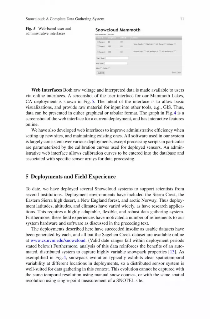
Fig. 5 Web-based user andadministrative interfaces

Web Interfaces Both raw voltage and interpreted data is made available to usersvia online interfaces. A screenshot of the user interface for our Mammoth Lakes,CA deployment is shown in Fig. 5. The intent of the interface is to allow basicvisualizations, and provide raw material for input into other tools, e.g., GIS. Thus,data can be presented in either graphical or tabular format. The graph in Fig. 4 is ascreenshot of the web interface for a current deployment, and has interactive featuresonline.

We have also developed web interfaces to improve administrative efficiency whensetting up new sites, and maintaining existing ones. All software used in our systemis largely consistent over various deployments, except processing scripts in particularare parameterized by the calibration curves used for deployed sensors. An admin-istrative web interface allows calibration curves to be entered into the database andassociated with specific sensor arrays for data processing.

5 Deployments and Field Experience

To date, we have deployed several Snowcloud systems to support scientists fromseveral institutions. Deployment environments have included the Sierra Crest, theEastern Sierra high desert, a New England forest, and arctic Norway. Thus deploy-ment latitudes, altitudes, and climates have varied widely, as have research applica-tions. This requires a highly adaptable, flexible, and robust data gathering system.Furthermore, these field experiences have motivated a number of refinements to oursystem hardware and software as discussed in the preceding text.

The deployments described here have succeeded insofar as usable datasets havebeen generated by each, and all but the Sagehen Creek dataset are available onlineat www.cs.uvm.edu/snowcloud. (Valid date ranges fall within deployment periodsstated below.) Furthermore, analysis of this data reinforces the benefits of an auto-mated, distributed system to capture highly variable snowpack properties [13]. Asexemplified in Fig. 4, snowpack evolution typically exhibits clear spatiotemporalvariability at different locations in deployments, so a distributed sensor system iswell-suited for data gathering in this context. This evolution cannot be captured withthe same temporal resolution using manual snow courses, or with the same spatialresolution using single-point measurement of a SNOTEL site.

12 C. Skalka and J. Frolik

Sagehen Creek Field Station, California, USA (Fall 2009–Spring 2010)Sagehen is situated just east of the Sierra Crest at an elevation of 2,000 m. Thedeployment period was December 2009 through June 2010. In addition to proto-type testing, this deployment was used for collaborative research with University ofNevada, Reno (UNR). The results of this research demonstrated that the combinationof telemetry obtained from a Snowcloud deployment, with models obtained usingstatistical techniques including linear regression and kriging, allows more accurateprediction of areal SWE averages than standard techniques [13]. This full-seasonfield campaign served to validate basic functionality and robustness of the Snow-cloud platform in its intended environment, and to demonstrate that our low-costultrasound-based approach to SD measurement specifically is effective.

The deployed network consisted of six sensor nodes, each supporting an aerialnode with temperature and ultrasound sensors. The deployment covered a 1 hectarelocation with variety of terrain and canopy features. As a field research station, wewere able to report data as it was collected, via the aforementioned collection treeprotocol (CTP), to a base station mote connected to a laptop in a laboratory buildingproximal to the deployment site. As this laptop was connected to AC power and theInternet, data was available in near-real-time and data collection and reporting neverfailed. As we discuss in the subsequent deployments, such convenience in reportingis not the norm in practice.

Mammoth Lakes, California, USA (Winter 2012-date) An active Snowcloudnetwork is currently deployed at an Easter Sierra Mountain site (elevation 2,300 m)near Mammoth Lakes. The data gathered by this network supports research directedby researchers from University of California, Santa Cruz (UCSC). The purpose ofthis research is to study the effects of climate change on alpine snow hydrologyand high-desert flora, specifically the effect of increased rain-on-snow events onshrub communities. This deployment consists of three towers deployed over a 300 mtransect, each with a fully-instrumented aerial node (SD, PAR and temperature) anda ground node (PAR, soil moisture at 10 cm and 1m). Leaf area index is derived fromthe difference between the PAR sensors in the aerial and ground arrays. Furthermore,the voltage sensor (discussed in technical detail in Sect. 2) provides useful systemtelemetry, i.e., an indication of battery levels over time. Both Harvester and Gatewaydevice prototypes have been utilized for data collection in this deployment.

Hubbard Brook Experimental Forest, New Hampshire, USA (Fall 2012-date)and Sulitjelma, Norway (Winter 2013-date) During the past year we have deployedthe Snowcloud system in two disparate but low altitude settings. The first site is on theforested slopes of the Hubbard Brook Experiment Forest in New Hampshire, USA(elevation 300 m). This area has been a site of a long term study to better understandsnow and its impact on streams and watersheds. This particular deployment supportsresearchers from the University of New Hampshire (UNH) who are studying theeffects of forest canopies on snow accumulation and melt. For this purpose we haveinstalled three towers with aerial nodes to provide continual sampling at sites wheremanual snow courses are conducted nominally on a biweekly basis. Our secondrecent deployment is outside the town of Sulitjelma, Norway in collaboration withresearchers at Stockholm University (SU). This site (elevation 150 m) is above the

Snowcloud: A Complete Data Gathering System 13

arctic circle which impacted greatly our ability to rely on solar for months during thewinter, and gave our system its most extreme test to date. We have four towers withaerial nodes at this site and a two-month sample of the collected snow depth data canbe seen in Fig. 4. The variability seen between towers deployed in near proximity(approximately 50 m apart) will help researchers develop more informative modelsfor areal SWE for the purposes of validating airborne data. The Harvester devicehas been successfully used by our collaborators to retrieve data from both of thesedeployments.

6 Conclusion

In this chapter, we have described the Snowcloud system for snow hydrology researchapplications, that implements a complete data collection pipeline from in situ sam-pling to online presentation. The main novelty of the system is its application space,and its design support for strategic short- and medium-term studies and adaptabilityto a variety of missions. The system has been successfully deployed in harsh Winterconditions in a number of settings, demonstrating the robustness of its design and theeffectiveness of distributed WSN technology for monitoring snowpack evolution.

As future work, we intend to expand applications of our system, and refine anddeploy our Gateway technology during the upcoming 2014 snow season. We alsointend to investigate network control algorithms to reduce system power consump-tion. These algorithms will leverage global knowledge and higher computing poweron the Gateway, and will build on so-called backcasting techniques [19] for net-work control and new programming languages technology for control orchestrationin WSNs [4]. Finally, we are working to augment Snowcloud with additional sens-ing capabilities including in situ temperature profiling and microwave attenuation tobetter characterize snowpack dynamics during melt onset.

Acknowledgments The authors express their thanks to our scientific collaborators, including DavidMoeser (Swiss Federal Institute for Snow and Avalanche Research—SLF), and Drs. Mark Walker(UNR), Michael Loik (UCSC), Jennifer Jacobs (UNH), and Ian Brown (SU). We would also liketo thank Dan Dawson (Sierra Nevada Aquatic Research Lab—SNARL) and Jeff Brown (SagehenCreek Field Station) for their invaluable support of our field work.

References

1. Alippi, C., Anastasi, G., Galperti, C., Mancini, F., Roveri, M.: Adaptive sampling for energyconservation in wireless sensor networks for snow monitoring applications. In: IEEE Confer-ence on Mobile Ad Hoc and Sensor Systems (2007)

2. Campbell, J., Ollinger, S., Flerchinger, G., Wicklein, H., Hayhoe, K., Bailey, A.: Past andprojected future changes in snowpack and soil frost at the Hubbard Brook Experimental Forest,New Hampshire, USA. Hydrol. Process. 24, 2465–2480 (2010)

14 C. Skalka and J. Frolik

3. Campbell, D. et al.: Attribution of declining Western U.S. snowpack to human effects. J. Climate105, 11826 (2008)

4. Chapin, P., Skalka, C., Smith, S., Watson, M.: Scalaness/nesT: type specialized staged pro-gramming for sensor networks. In: ACM Generic Programming: Concepts and Experiences(GPCE) (2013)

5. Franz, K., Hatmann, H., Sorooshian, S., Bales, R.: Verification of national weather serviceensemble stream-flow predictions for water supply forecasting in the Colorado River basin. J.Hydrometeorol. 4, 1105–1118 (2003)

6. Guizzo, E.: Into deep ice. IEEE Spect. 42(12), 28–35 (2005)7. Hasler, A., Talzi, I., Tschudin, C., Gruber, S.: Wireless sensor networks in permafrost research—

concept, requirements, implementation and challenges. In: Proceedings of 9th Int’l Conferenceon Permafrost (2008)

8. Henderson, T., Grant, E., Luthy, K., Cintron, J.: Snow monitoring with sensor networks. In:IEEE International Conference on Local Computer Networks (2004)

9. Kerkez, B., Glaser, S., Bales, R., Meadows, M.: Design and performance of a wireless sensornetwork for catchment-scale snow and soil moisture measurements. Water Resour. Res. 48(9),w09515 (2012)

10. Lampkin, D.: Resolving barometric pressure waves in seasonal snowpack with a prototype-embedded wireless sensor network. Hydrol. Process. 24, 2014–2021 (2010)

11. Liston, G.: Interrelationships among snow distribution, snowmelt, and snow cover depletion:implications for atmospheric, hydrologic, and ecologic modeling. J. Appl. Meteorol. Climatol.38, 1474–1487 (1999)

12. MEMSIC.: TelosB data sheet. Technical report, 6020–0094-03 Rev A (2013)13. Moeser, C., Walker, M., Skalka, C., Frolik, J.: Application of a wireless sensor network for

distributed snow water equivalence estimation. In: Western Snow Conference (2011)14. NOAA.: Strategic science plan. Technical report, Office of Hydrologic Development Hydrology

Laboratory (2007)15. Tedesco, M., Narvekar, P.: Assessment of the NASA AMSR-E SWE product. IEEE J. Sel. Top.

Appl. Earth Obs. Remote Sens. 3(1), 141–159 (2010)16. UNESCO.: Third UN world water development report: water in a changing world. Technical

report, UN (2007)17. Vilajosana, I., Llosa, J., Schaefer, M., Surinach, E., Marques, J.M., Vilajosana, X.: Wireless

sensors as a tool to explore avalanche internal dynamics: experiments at the Weissfluhjochsnow chute. In: International Snow Science, Workshop (2009)

18. Welles, E., Sorooshian, S., Carter, G., Olsen, B.: Hydrologic verification: a call for action andcollaboration. Bull. Amer. Meteor. Soc. 88(4), 503–511 (2007)

19. Willett, R., Martin, A., Nowak, R.: Backcasting: adaptive sampling for sensor networks. In:IPSN, pp. 124–133 (2004)

20. Yan, F., Ramage, J., McKenney, R.: Modeling high-latitude spring freshet from AMSR-Epassive microwave observations. Water Resour. Res. 45, w11408 (2009)

The Big Night Out: Experiences from TrackingFlying Foxes with Delay-Tolerant WirelessNetworking

Philipp Sommer, Branislav Kusy, Adam McKeownand Raja Jurdak

Abstract Long-term tracking of small-size animals with wireless sensor networksremains a challenge as only limited energy harvesting and storage is possible due tostringent size and weight constraints for animal collars. We present first experiencestowards a perpetual monitoring system for free-living flying foxes. The high mobilityof flying foxes requires a delay tolerant wireless network for data gathering: GPSpositions and sensor data have to be stored locally until a wireless gateway deployedin bat congregation areas, so called roosting camps, comes within radio range. Inthis chapter, we present the system architecture and discuss our design decisionstowards sustainable and reliable monitoring of flying foxes with a limited energybudget for sensing, storage and communication. Using empirical data from threefree-living flying foxes, we characterize the overall system performance in terms ofenergy consumption and latency.

1 Introduction

The ongoing technological innovation, driven by the explosion of interest in mobilephone technology, has led to ever smaller, less energy demanding, and more accuratesensors and computation devices available on the market. Modern smart phones can

P. Sommer (B) · B. Kusy · R. JurdakAutonomous Systems Lab, CSIRO Computational Informatics,Brisbane, QLD, Australiae-mail: philipp.sommer@csiro.au

B. Kusye-mail: brano.kusy@csiro.au

A. McKeownCSIRO Ecosystem Sciences, Cairns, QLD, Australiae-mail: adam.mckeown@csiro.au

R. Jurdake-mail: raja.jurdak@csiro.au

K. Langendoen et al. (eds.), Real-World Wireless Sensor Networks, 15Lecture Notes in Electrical Engineering 281, DOI: 10.1007/978-3-319-03071-5_2,© Springer International Publishing Switzerland 2014

16 P. Sommer et al.

localize users with an accuracy of a few meters, thus enabling novel applications thatwould not have been possible a few years ago. Decreasing form factor, weight, costand energy consumption have made GPS receivers a versatile research tool enablingnovel applications across several domains.

Wireless sensor networks (WSNs) are well suited for wildlife habitat monitoringapplications. Sensor nodes, also called motes, combine sensing, processing, storage,communication, and energy harvesting capabilities in a small and light-weight pack-age powered by batteries. Researchers typically place motes at specific locationsto deliver non-intrusive long-term observation of natural habitats. However, manyresearch questions require tracking the movements of individual animals within apopulation at high spatial and temporal resolution [3, 5, 9]. Recently, GPS-enabledcollars weighting just above 100 g have been used for long-term tracking of Whoop-ing Crane migration in North America [1]. As maximum weight of a collar is usuallylimited to 5 % of the body weight of the animal, tracking small-size animals remainsa challenge.

Application context Flying foxes are mammals that belong to the family of fruitbats (Pteropididae). They are common in the tropic and subtropic areas of Asia,Australia and Pacific Islands. They congregate in large numbers of up to severalthousands individuals to roost during daytime in so called camps. Flying foxes arenocturnally active and leave the camps for foraging from fruit trees. During thenightly foraging, they are able to cover distances up to 100 km over more than 10 h.Monitoring mobility and behavior of individual flying foxes is motivated by the needto better understand this threatened species. Furthermore, flying foxes are attributedto carry diseases, such as the Hendra or Lyssa viruses, which can be transmitted toother animals or humans.

Challenges Developing a hardware and software system to track flying foxes ischallenging due to several constraints. First of all, animal ethics requires that thecollar accounts for less than 5 % of the animal’s body weight. Depending on the typeof animal and differences in body weight between male and female individuals, thisresults in a total weight limit of 30 to 50 g for all electronic components, small solarpanels and batteries. Consequently, we are severely limited in terms of availableenergy resources required to perform sensing, processing, storage and communi-cation tasks. Second, our goal is to track free-living animals, so we will have nophysical contact with the collar after the deployment time. Finally, flying foxes leavethe camp for a period of more than 10 h every night and can be away for multipledays. Collars need to collect data in a delay-tolerant way and operate for long periodsof time during which they cannot communicate with the base station.

Contributions In this work, we present the system architecture and discuss ourdesign decisions to achieve perpetual low-power operation of a tracking device(Sect. 2). First, we have developed BatMac, a simple scheduling algorithm for low-power wireless communication tailored to our particular application domain. Specifi-cally, a large number of animals congregate within the relatively small area of a campduring daytime, which allows for offloading previously gathered sensor data to a basestation. We use a slotted schedule based on GPS time to desynchronize transmissions

The Big Night Out: Experiences from Tracking Flying Foxes 17

Base station 1 Base station 2 Base station nServer

Fig. 1 The network architecture of the Bat Monitoring Project

of individual collars and use a simple radio duty-cycling approach that assumes analways-on base station (Sect. 3). Second, profiling and debugging of wireless sensornodes on free-living animals paired with the intermittent radio connectivity is a chal-lenging task. We have implemented a scheduler that guards execution of individualsensing tasks and use several mechanisms to improve software and hardware reli-ability. We also implemented an over-the-air reconfiguration protocol that helps tomitigate the lack of physical access to the device after the deployment time (Sect. 4).Finally, we use empirical data from three flying foxes to demonstrate performanceof individual system components in real-world deployments.

2 System Architecture

In this section, we give a brief overview of the system architecture, shown in Fig. 1.Our wireless sensor network consists of three layers: (1) the mobile sensing nodesintegrated into an animal collar deployed on flying foxes, (2) the base station layerwhich consists of several spatially distributed units, and (3) the central databaseserver.

2.1 Mobile Sensing Layer

The purpose of the mobile sensing device is to gather sensor data from an individualcollared animal using a variety of sensors (e.g., GPS, accelerometer, pressure sensor).The mobile sensor device is housed inside a collar, which can be attached around theanimal’s neck by experts trained in handling flying foxes.

In order to meet the stringent constraints in terms of weight, size and powerconsumption, we decided to build our own printed circuit board (PCB). A detaileddescription of this board is available in [8]. The software on the mobile sensor nodeis running a modified version of the Contiki operating system that adds customextensions for logging and remote procedure calls (RPC) (see Sects. 3 and 4).

18 P. Sommer et al.

2.2 Base Station Layer

Bat roosting camps provide an ideal opportunity for the placement of static infrastruc-ture, so called base stations, as thousands of animals congregate within a relativelysmall area during daytime. The base station is responsible for downloading sensordata from nearby mobile nodes by using short-range wireless connectivity. We use agateway node with a TI CC1101 radio connected to an embedded Linux system forcontrol and monitoring of the download operations. In addition, a 2G/3G wirelessmodem connects the base station to our central server for data uploads. We employsolar panels and batteries to allow autonomous operation in bat camps. Solar energyharvesting is usually a reliable source of power in tropical or subtropical locationswith plenty of sunshine, but consecutive days with cloud cover or dense vegetationcan limit the amount of solar energy harvested. Consequently, we might only be ableto operate the base station during a limited time and have to batch downloading datafrom animals and uploading to the database.

2.3 Backend Storage and Control Layer

Sensor readings from different mobile nodes are downloaded by spatially separatedbase stations and transferred to a central database for permanent storage and offlineanalysis. The database is further responsible to keep a synchronized view of whichpages have been already downloaded from nodes. This information is required toavoid duplicate downloads of the same page when the animal is roaming betweendifferent camps. Network health data such as battery voltage and number of packetsreceived from different base stations are periodically reported to the database to assistin continuous monitoring and network management.

3 Delay Tolerant Networking for Animal Tracking

Flying foxes are known to cover large distances during nightly foraging and seasonalmigrations between different camps. Satellite-based communication systems allowdata upload at global scale but pose a significant burden in terms of their cost, size andpower consumption. The large spatial coverage of cellular communication networks(e.g., 2G and 3G systems) offers a flexible and cost effective alternative to satellitebased systems. However, size and power hinders the integration into collars for smallmammals and birds with more stringent constraints. Therefore, we have opted for alow-power, short-range wireless transceiver (TI CC1101) that allows energy efficientoperation within unlicensed bands of the frequency spectrum. The disadvantage ofour approach is the need to maintain the infrastructure of base stations in flying-foxcongregation areas.

The Big Night Out: Experiences from Tracking Flying Foxes 19

Protocols for data collection During the last decade, several data collection pro-tocols for wireless sensor networks have evolved for different application scenarios.Data collection protocols such as CTP [7] and Dozer [2], maintain a routing tree alongwhich packets are forwarded towards the sink node. While both protocols are ableto duty-cycle the radio transceivers to save energy, maintaining the network staterequires periodic radio beacons. Recently, several communication protocols havebeen proposed that not need to keep topology-dependent state, such as the Low-Power Wireless Bus [6], which are resilient to high node mobility, but require thenodes to maintain accurate synchronization.

3.1 The BatMac Protocol

Given the uncontrolled mobility patterns of free-living animals and limited energyresources for wireless communication, we decided to implement a novel protocolcalled BatMac. BatMac is a time-synchronized medium access protocol, which istailored to the intermittent connectivity between mobile nodes and the base station.BatMac is a sender-initiated single-hop protocol implemented on top of Contiki’sRIME network stack. It is based on the observation that, unlike homogeneous sensornetworks, the distribution of power budgets is highly asymmetric in our network.Mobile nodes can aggressively duty-cycle their radios while the base station operatesits radio continuously. Therefore, we do not to use multi-hop communication forpacket forwarding, which allows mobile receivers to put their radio in sleep modefor long periods of time.

Slotted communication We use a combination of time-based communicationslots and a request-response protocol to avoid interference when multiple mobilenodes are present within communication range of a single base station. Mediumaccess is scheduled using a concept of communication rounds that each consistof several sub-slots. Nodes can access the radio channel exactly once during eachcommunication round, in a sub-slot that is determined by their node ID. For example,for a system with 10 nodes, we might define a communication round to take 5 minand consist of 10 sub-slots. Each of the 10 nodes will then transmit once every 5 minfor up to 30 s.

Timings of rounds and sub-slots are determined based on UTC time tracked by thereal-time clock of mobile nodes. The real-time clock is periodically re-synchronizedon every GPS lock. The mapping between nodes and their corresponding sub-slotis based on their unique identifier. Selection of the round length and the number ofsub-slots is a tradeoff between data transmission latency and the maximum numberof nodes that we support. As our deployment needs to scale up to 1000 nodes ormore, we can assign multiple nodes to the same slot through a modulo operation ontheir node IDs. We synchronize the real-time clock to within a second to the GPStime, which has the effect of randomizing transmission of beacons within the samesub-slot.

20 P. Sommer et al.

Announcement beacon Each mobile node periodically broadcasts a radio packetcontaining an announcement beacon at the beginning of its designated communica-tion slot. The announcement contains the node’s identifier, application version, andthe current flash page number. After sending the radio packet, the node keeps itsradio on until a predefined timeout (e.g., 1 s) expires. If the timeout expires, the radiois switched off until the next announcement.

Node selection The base station is continuously listening for incoming announce-ment beacons from mobile nodes. Upon reception of an announcement, the basestation determines if further communication with the node is required, e.g., if newdata needs to be downloaded from the flash or the node’s configuration should beupdated. If further communication is needed, the base station keeps the node’s radioawake, by sending aradio_on(timeout) command, which will set a new timeoutto switch off the radio at the node.

3.2 Data Storage

We are interested in collecting sensor readings from different sensors while the collaris on the animals for several weeks, months or years. Mobility patterns of free-livinganimals make it very difficult to predict when the animal will be nearby a campwhere a base station is deployed. Thus, our software is required to provide persistentstorage of sensor data for several hours, days or even weeks. We implemented a first-in first-out data store using the external flash as a circular buffer. Our AT25DF641flash chip is divided in 32768 pages of 256 bytes each.

The variety of sensors on the mobile device requires a data storage system thatis able to handle readings of different payload sizes and at different data rates. Forexample, a single GPS reading includes values for the timestamp, latitude, longitude,height, speed and an estimation of position accuracy, which results in a total of15 bytes every second. On the other hand, the combined 3-axis accelerometer andmagnetometer sensor generates 12 bytes per reading and can operate at samplingrates up to 100 Hz.

Tagged data format We adapt the Tagged Data Format (TDF) from [4] to packsensor readings into a byte stream. TDF adds metadata such as the sensor type andtimestamp in front of each reading (see Fig. 2). The ID of the sensor type and flagsindicating the type of timestamp (relative or absolute) are encoded into a 2-byteheader field. Sensor readings associated with an absolute timestamp need 6 bytes toencode the seconds (4 bytes) and millisecond fraction (2 bytes) of the timestamp. Ifthe timestamp of the current reading can be encoded using an offset to the previoustimestamp, it is only necessary to store a 2-byte offset. Each sensor type has a specificlength for sensor readings, which is fixed and needs to be known to both the encoderand decoder of a TDF stream. To enable decoding of each flash page individually,the first sensor reading always uses an absolute timestamp.

The Big Night Out: Experiences from Tracking Flying Foxes 21

Sensor Type+ Flags2 bytes

Timestamp(global)

Sensor Data

6 bytes 1..n bytes

Sensor Type+ Flags2 bytes

Timestamp(offset)

Sensor Data

2 bytes 1..n bytes

Sensor Type+ Flags2 bytes

Timestamp(offset)

Sensor Data

2 bytes 1..n bytes

Fig. 2 Storage of sensor readings in flash using the tagged data format (TDF)

Evaluation TDF is a flexible format that provides a compact representation ofheterogeneous sensor readings in flash storage. However, the TDF encoder has tojump to the next page if not enough bytes are available in the remainder of the flashpage. This fragmentation leads to empty bytes at the end of a page. We characterizethe overhead of encoding sensor readings using TDF on sensor data from a collarattached to a free-living flying fox. We downloaded 1147 pages from the flash storageof the node and analyzed 17730 sensor readings encoded in the TDF stream. Ourresults indicate that the actual sensor data accounts for 65 % of the flash page sizeof 256 bytes, while headers account for 12 % (sensor type) and 19 % (timestamp).Finally, the overhead due to empty bytes at the end of a flash page accounts for only4 % of the flash size, which is acceptable given the flexibility that TDF offers forstoring heterogeneous sensor data into a continuous flash buffer.

3.3 Data Retrieval

Data downloads are initiated by the base station as a response to an announcementbeacon, based on the node’s current flash page number contained in the beacon.The download handler runs as a Python script on the embedded Linux machine. Weimplemented a greedy approach to scheduling downloads from nodes within radiorange of a base station. If the current page number in the beacon is higher thanthe last downloaded page, the base station requests missing pages from the node insequential order.

Since a full page of 256 bytes would not fit into a single radio packet, we useRPC calls to request chunks of bytes within a specific page from the base. EachRPC command is retransmitted up to 5 times if not acknowledged by the node. If acomplete page has been transferred, the base reassembles it and decodes its contentusing the TDF parser. If the page contains no errors, the base will upload the sensordata to the central database server and mark the corresponding page as complete. Ifno Internet connection is available at the base station, data will be buffered locallyat the base until it can be uploaded to the database.

Data consistency The request/response approach requires the base station to knowthe latest information from each node that is stored in the database. Since our systemarchitecture includes multiple spatially distributed base nodes, we use a centralizedapproach to coordinate data downloads across the base stations. Base stations keeptrack of the most recently downloaded flash page for every mobile node, whichallows mobile nodes not to keep track of the download process. Mobile nodes needto simply announce their most recent flash page number and then respond to a base

22 P. Sommer et al.

Beacon

Day 1 Day 2 Day 3 Day 4 Day 5 Day 6 Day 700 06 12 18 00 06 12 18 00 06 12 18 00 06 12 18 00 06 12 18 00 06 12 18 00 06 12 18 00

0200400600800

100012001400

Pag

es

Data acquisitionData download

Fig. 3 Timeline of received radio announcement packets at the base station from a single bat (top)and the number of generated versus downloaded flash pages (bottom)

station’s RPC to transmit a specific flash page. Each page will only be downloadedexactly once as long as the state information is synchronized across all base stations.However, this needs to be done only every couple of hours as animals are unlikelyto move between the spatially separated base nodes within that time window.

Evaluation We present experimental results using data downloaded from a singlewild bat during a 7-day period. Figure 3 shows received announcement packets andnumber of pages written to flash. In general, we are able to receive announcementbeacons from the mobile node just before 6 am in the morning until just after 6 pmin the evening. In the morning, the earliest received beacon was at 5.34 am on thesecond day while no beacons were received until 6.14 am on Day 4. The last beaconfrom the animal was received between 5.09 (Day 1) and 6:19 pm (Day 5, 6 and 7). Wecalculate the packet reception rate (PRR) for announcement beacons as the fractionbetween received beacons and the number of expected beacons between the first andlast received beacon for every day. The range of the observed PRR is between 0.35(Day 5) and 0.78 (Day 2).

By analyzing the timestamps embedded in the downloaded pages, we are able totrack the flash storage consumption over time. Flash pages are written at a lower rateduring daytime, as we are mainly logging node health information and a few GPSpositions. The data rate increases between 6 pm and 6 am when high-frequency GPSsampling is activated. The latency between data acquisition and download is lowduring the day since the base station is able to download new pages continuously.Clearly, the latency is higher for data gathered during the night as we have up to12 h without contact to the base station. Depending on the quality of the radio link inthe camp, it might take several hours until the nightly backlog is downloaded (e.g.,Day 5).

4 Configuration and Debugging

Development of hardware and software for animal tracking is challenging due tothe mobility of the animals. While it is relatively easy to follow the path of col-lared livestock, catching and collaring of free-living animals such as flying foxes islabor intensive and notoriously difficult. Large nets mounted between high poles arerequired to catch animals while they are flying back in or out of the camp during

The Big Night Out: Experiences from Tracking Flying Foxes 23

the night. Catching a collared animal a second time is almost impossible given thelarge number of individuals populating a camp. Therefore, our development approachassumes that it is not possible to gain physical access to the mobile node ever againafter the initial deployment.

4.1 Remote Task Configuration

Several mechanisms for over-the-air code distribution in wireless sensor networkshave been proposed in the literature. However, supporting wireless reprogrammingincreases the complexity of the code running on the node and requires dedicatedstorage for new and fallback images. Furthermore, any failure during the reprogram-ming process might leave the node in a defective state. Therefore, we decided not toimplement over-the-air reprogramming for our mobile nodes. Instead, we integratedmethods to support wireless reconfiguration for a set of well-tested tasks within ourapplication. Each task is associated with a Contiki process that implements a specificsensing task (e.g., getting several GPS fixes, or measuring the battery voltage). Taskscan be limited to a specific time interval (start, stop), periodicity within that timeinterval, and minimum battery voltage. Tasks can also have additional argumentswhich are specific to a sensor (e.g., number of samples). The task scheduler is exe-cuted once every second to start or stop tasks according to the current configuration.

Reconfiguration Task configurations use a dedicated part of the flash for persis-tent storage. We provide remote procedure calls (RPC) sent over the radio to view,update and delete a task on the sensor node.

4.2 Remote Debugging

We implemented two methods for debugging mobile nodes deployed on animals:Node inspection by remote procedure calls sent over the radio, and logging of debugoutput to the flash storage as part of TDF data. In addition, we use a combination ofhardware and software based mechanisms to recover from error conditions. In theremainder of this section, we describe the debugging capabilities integrated with ourapplication and highlight how their usefulness for debugging in practice.

Node inspection We implemented several helper methods for debugging andinspection of the current node state. Thereby, we do not want to halt code executionon the node, but rather acquire a snapshot of the node’s status, e.g., the current valueof a variable in RAM. Furthermore, custom RPC methods allow us to reboot the node,sample the battery voltage, read data from the external flash, and read/modify/deletetasks.

Debug instrumentation While RPC methods are useful to inspect the node statuswhen radio connectivity is available, little information is available during periods

24 P. Sommer et al.

with no radio connectivity. Therefore, we implemented two additional sensing tasksuseful to aid the process of debugging. The POWER task will periodically sample thebattery voltage, solar panel voltage, and charge current and write the ADC readingsto the flash storage using the TDF logging abstraction. In addition, the DEBUG taskperiodically logs the reason for the last microcontroller reset and the current uptime inseconds, allowing us to track node reboots and determine their cause retrospectively.

Watchdog and Grenade timers We combine a hardware watchdog and a softwaretimer to recover from potential problems that could cause the software running onthe microcontroller to get stuck. The hardware watchdog of the MSP430 will triggera reboot if the watchdog timer is not being reset within 2 s. Therefore, we instrumentContiki’s main scheduler loop to reset the watchdog periodically. This mechanismwill protect us from possible software errors within the implementation of our Contikiprocesses such as infinite loops. A so called grenade timer is used as an additionallayer of protection against hardware and software problems. Thereby, we force agraceful node reboot when the uptime counter reaches a predefined value (e.g., oncea day). Grenade reboots can easily be distinguished from uncontrolled reboots bylooking both at the reset reason and the value of the uptime counter logged to flash.

5 Experimental Data: A Day in the Life of a Flying Fox

We present preliminary experimental results from two mobile nodes attached tofree-living flying foxes. Both animals left the camp during the night and returnedat dawn. We configured two different tasks for GPS sampling to gather the positionof the mobile node depending on the current time of day. The low-frequency GPStask will log the current location every 3 h during the day. During the night, thehigh-frequency GPS task logs locations every 10 min.

5.1 GPS Tracking

The interval between startup of the GPS receiver until the first GPS position isavailable is commonly denoted as the Time to First Fix (TTFF). During a coldstart,the GPS receiver has to search for a signal from several GPS satellites to determine itscurrent position. After the first valid position has been calculated, the receiver keepstracking the existing satellites in order to periodically update its estimation of thecurrent location. We use the sleep mode of the u-blox MAX6 module, which retainsreal-time clock and satellite orbit information while the main part of the receiver isput into a low-power mode. A GPS hotstart is possible if the receiver wakes up fromsleep mode and has up-to-date satellite information to calculate the current position,otherwise, it has to go through a coldstart phase again. We collected TTFF values of1103 successful GPS location requests from two nodes. Reported values for TTFF

The Big Night Out: Experiences from Tracking Flying Foxes 25

0 10 20 30 40 50 60 70Time to First Fix [s]

0.000.050.100.150.200.250.300.35

Fre

quen

cy

0 10 20 30 40 50 60 70Time to First Fix [s]

0306090

120150180

GP

S o

ff-tim

e [m

inut

es]

Fig. 4 Distribution of the time to first GPS fix (left) and the relation between the preceding GPSoff interval and the time to first fix (right)

are between 1 and 67 s while it takes 4.17 s to get the first valid position on average(see Fig. 4). We further observe that it takes longer to get the first fix when the GPSwas inactive for a longer period of time.

5.2 Power Management

The amount of remaining energy stored in the rechargeable battery depends on sev-eral factors, such as the amount of solar energy harvested and the current draw duringrecent days. We periodically measure the battery voltage, the solar panel voltage andthe charge current into the battery using the on-board ADC on the sensor node. Whilewe aim to derive an accurate estimation for the remaining energy based on measure-ments in future versions, the task scheduler currently only uses the battery voltagewhen deciding whether to execute a task. Power measurements and correspondingGPS task execution times are reported in Fig. 5. We measure similar values for thecharge current for both nodes. We see considerable differences between the twomobile devices, although the animals are roosting in the same camp. Node A main-tains a relatively stable battery voltage across the whole measurement period whilethe battery voltage of Node B decreases rapidly during the night time. As a resultof the low voltage, Node B stops gathering GPS samples as its battery drops belowthe threshold voltage. We can also see a significant difference between rainy weather(Day 1) and sunny weather (Days 2 to 5). Furthermore, we continually increase theduty-cycle of the GPS task during the night. Starting from fixes every 10 min between6 pm and 6 am (Day 1/2), we extended the window from 5.30 pm to 6 am to capturethe departure of the animals from the camp (Day 3/4). Finally, we reconfigured theGPS task to gather continuous GPS fixes at a frequency of 1 Hz between 5.35 and6 pm on the evening of Day 5. Figure 6 shows the positions of the animals on a map.

26 P. Sommer et al.

GPS

Day 1 Day 2 Day 3 Day 4 Day 500 06 12 18 00 06 12 18 00 06 12 18 00 06 12 18 00 06 12 18 00

Time

3.3

3.53.73.9

Batte

ry [V

]

GPS thresholdBattery Voltage

Charge Current05101520

Cha

rge

Cur

rent

[mA]

GPS

Day 1 Day 2 Day 3 Day 4 Day 500 06 12 18 00 06 12 18 00 06 12 18 00 06 12 18 00 06 12 18 00

Time

3.33.53.73.9

Batte

ry [V

]

GPS threshold

Battery Voltage

Charge Current0510152025

Cha

rge

Cur

rent

[m

A]

Fig. 5 Battery voltage, charge current and activation of the GPS task for Node A (top)and B (bottom)

Node B: 17:45

Node A: 17:45

Camp Location

Node A: 05:55

Node A: 17:50

Node A: 05:50

Node A: 17:55

Node A: 05:45

Node A: 18:00-05:40

Node B: 17:50

Node B: 17:55-18:55 19:35-00:55

Node B: 19:00

Camp Location

Node A: 17:38

Node A: 17:56-05:50

Node B: 18:00-19:10

Node B: 17:57

Node B: 17:43

Fig. 6 GPS waypoints of two mobile nodes: The GPS was configured to get fixes every 10 minduring night time on Day 4 (left). Continuous sampling allows to track the accurate flight path whenanimals leave the camp on Day 5 (right)

6 Lessons Learned

In this chapter, we have presented our first experience with a novel hardware and soft-ware architecture for monitoring flying foxes using mobile sensor nodes. Althoughthis project is only at an early stage and deployment of several hundred animal

The Big Night Out: Experiences from Tracking Flying Foxes 27

collars is planned over the next months, we have gathered a large set of empiricaldata, which allows us to verify the correctness of system operations and providesinvaluable information for fine-tuning our system in future deployments.

We believe that staggered releases of new software features to a small numberof nodes can mitigate the impact of possible software problems instead of rollingout several hundred nodes simultaneously. However, this requires co-existence ofdifferent software versions, as collars with older software versions still remain active.Thus, we assign a software version to each node which is also included as part ofthe announcement beacon, enabling to identify the capabilities of different nodes.Furthermore, diagnostic tools built on top of remote procedure calls enable flexibleinspection of nodes within range.

Logging state information to persistent storage is vital for debugging a system withintermittent network connectivity. The over-the-air reconfiguration of tasks providescontrol over the amount of debug output during different stages of the deployment,thus providing code instrumentation only when needed.

Acknowledgments We would like to thank Ben Mackey, Philip Valencia, Chris Crossman, LukeHovington, Les Overs and Stephen Brosnan for their contributions to this project.

References

1. Anthony, D., Bennett, W., Vuran, M., Dwyer, M., Elbaum, S., Lacy, A., Engels, M., Wehtje,W.: Sensing through the continent. In: ACM/IEEE IPSN (2012)

2. Burri, N., von Rickenbach, P., Wattenhofer, R.: Dozer: Ultra-low power data gathering in sensornetworks. In: ACM/IEEE IPSN (2007)

3. Butler, Z.: From robots to animals: virtual fences for controlling cattle. J. Robot. Res. 25, 5–6(2006)

4. Corke, P., Wark, T., Jurdak, R., Moore, D., Valencia, P.: Environmental wireless sensor net-works. Proc. IEEE, 98(11), (2010)

5. Dyo, V., et al.: WILDSENSING: design and deployment of a sustainable sensor network forwildlife monitoring. ACM Trans. Sens. Netw.8(4), (2012)

6. Ferrari, F., Zimmerling, M., Mottola, L., Thiele, L.: Low-power wireless bus. In: ACM SenSys,(2012)

7. Gnawali, O., Fonseca, R., Jamieson, K., Moss, D., Levis, P.: Collection Tree Protocol. In: ACMSenSys, (2009)

8. Jurdak, R., Sommer, P., Kusy, B., Kottege, N., Crossman, C., Mckeown, A., Westcott, D.:Camazotz: multimodal activity-based GPS sampling. In: ACM/IEEE IPSN, (2013)

9. Zhang, P., Sadler, C.M., Lyon, S.A., Martonosi, M.: Hardware design experiences in ZebraNet.In: ACM SenSys (2004)

On Rendezvous in Mobile Sensing Networks

Olga Saukh, David Hasenfratz, Christoph Walser and Lothar Thiele

Abstract A rendezvous is a temporal and spatial vicinity of two sensors. In thischapter, we investigate rendezvous in the context of mobile sensing systems. Weuse an air quality dataset obtained with the OpenSense monitoring network toexplore rendezvous properties for carbon monoxide, ozone, temperature, and humid-ity processes. Temporal and spatial locality of a physical process impacts the numberof rendezvous between sensors, their duration, and their frequency. We introduce arendezvous connection graph and explore the trade-off between locality of a processand the amount of time needed for the graph to be connected. Rendezvous graphconnectivity has many potential use cases, such as sensor fault detection. We suc-cessfully apply the proposed concepts to track down faulty sensors and to improvesensor calibration in our deployment.

1 Introduction

In recent years, wireless sensor networks (WSNs) have become a mature technologyand are successfully used in a number of long-term installations [1, 2]. Most deploy-ments are composed of static sensors fixed at desired locations, which are carefullychosen according to the node’s communication and sensing ranges. The data mea-sured by such deployments is usually highly temporally resolved at every chosen

O. Saukh (B) · D. Hasenfratz · C. Walser · L. ThieleComputer Engineering and Networks Laboratory, ETH Zurich, Zurich, Switzerlande-mail: saukh@tik.ee.ethz.ch

D. Hasenfratze-mail: hasenfratz@tik.ee.ethz.ch

C. Walsere-mail: walser@tik.ee.ethz.ch

L. Thielee-mail: thiele@tik.ee.ethz.ch

K. Langendoen et al. (eds.), Real-World Wireless Sensor Networks, 29Lecture Notes in Electrical Engineering 281, DOI: 10.1007/978-3-319-03071-5_3,© Springer International Publishing Switzerland 2014

30 O. Saukh et al.

location. The main drawback of static installations is, however, their poor spatialscalability to monitor large areas. Involvement of mobile sensor nodes increasesspatial area coverage at the price of temporal coverage. Additionally, it enables ape-riodic rendezvous between sensors. We define a rendezvous as a temporal and spatialvicinity of two sensors. A rendezvous is not bounded to a specific location in timeand space. In fact, two sensors moving around hand in hand build one rendezvouswith infinitely many temporally and spatially related measurements.

Despite the advantages of mobile sensors, ensuring faultless operation [3, 4],automatic sensor calibration [5, 6], and data quality (e.g., by timely detection ofoutliers [7]) are challenging tasks in mobile networks due to the sporadic and unpre-dictable nature of rendezvous. Additionally, access to reliable reference measure-ments is absent or limited to a small number of locations. Thus, supervising theerror-free operation of mobile sensor networks is only possible by either carefullydesigning and exploiting rendezvous between sensors, or applying model-based datavalidation schemes. The latter requires models describing the phenomenon of interestand sensors in use, which are typically not known a priori [8] and hard to obtain[9, 10].

In many urban areas, public transport vehicles, such as streetcars and buses,provide a suitable basis for deploying wireless sensor nodes [11]. The inherent mobil-ity in such installations often solves spatial coverage problems and enforces highprobability of rendezvous due to a usually good connectivity of public transport net-works (PTNs). We monitor airborne pollutants and environmental parameters withthe OpenSense nodes, which are installed on top of public streetcars traversing thecity of Zurich, Switzerland.

In this chapter, we use our deployment to implement an in-depth analysis ofrendezvous between mobile sensor nodes to ensure consistent network operation, andinvestigate prerequisites and limits of this approach. To the best of our knowledge,this is the first chapter researching this direction. The presented results are basedon data obtained from three months of operation gathering more than 4 millionsmeasurements.

Past research efforts on exploiting rendezvous in mobile networks focused ondata communication [12–15] and network-wide time synchronization [16]. In bothcases, a rendezvous depends on the node’s communication range and is assessedin terms of successful communication between two nodes. This definition is binary,since communication either succeeds or fails. Many environmental monitoring appli-cations would leverage a phenomenon-based definition of rendezvous for their usein sensor calibration and sensor failure detection routines [17, 18]. However, giventemporal and spatial distances between two sensors, what can be concluded aboutthe similarity of their respective measurements? How close should two sensors cometogether so that one can expect their measurements to be similar? In this chapter, wemake use of our dataset to shed light on these questions.

Contributions and Roadmap Different phenomena exhibit different notions ofspatial and temporal locality. Once two sensors are in close vicinity of each other,they are expected to deliver similar measurements. In this chapter, we propose aphenomenon-based definition of a rendezvous, which exploits this property using air

On Rendezvous in Mobile Sensing Networks 31

pollution measurements from our mobile OpenSense nodes traversing a large urbanarea of 100 km2.

The main contributions described in this chapter are:

• We introduce the notion of a rendezvous based on the spatial and temporal localityof a phenomenon. Using the OpenSense dataset, we can clearly distinguish global(temperature and humidity) from more local (carbon monoxide) phenomena.

• We construct a rendezvous connection graph, which enables comparing any pair ofsensors in the network. We explore the trade-off between locality of a phenomenonand time required to achieve connectivity in the rendezvous connection graph. Wefind that in our deployment connectivity is achieved within a few days even forlocal phenomena, such as carbon monoxide dispersion in an urban environment.

• We demonstrate the applicability of rendezvous to detect sensor failures and toimprove sensor calibration in the running OpenSense deployment.

We summarize related work in Sect. 2. In Sect. 3 we present the OpenSense deploy-ment and describe the dataset used in Sect. 4 to explore the properties of rendezvous.The determined rendezvous parameters for a number of environmental phenomenaare used in Sect. 5 to detect faulty sensors and update sensor calibration. We concludein Sect. 6.

2 Related Work

Two directions in WSN research are related to the contributions of this chapter:exploiting node rendezvous in mobile networks and characterization of sensors’sensing ranges. Many applications of mobile networks leverage node rendezvousfor data communication [12] and time synchronization [16]. A large body of workexplores temporal connectivity in opportunistic networking, e.g. [19]. Several worksadvocate data muling to minimize node energy consumption by gathering data witha mobile sink [13–15]. The resulting communication range based rendezvous aredefined by a successful communication link and are thus binary in contrast to sensingrange based rendezvous.

Unit disc graph model [20] of a sensing range is a popular assumption in a greatbody of theoretical publications. Although this model is rather simplistic, it is widelyused for theoretical analysis and algorithm design. In particular, many early coverageand k-coverage scheduling algorithms are based on this model [17, 21–24]. Theseworks often either ignore the deviation of the model from reality or assume that thesensing radius can be obtained. A few works even propose to calibrate the sensingrange to fit specific requirements [25, 26].

More recent research activities explore diversity of sensing ranges and buildalgorithms that are not limited to any specific model. In [27], the authors developedan energy efficient node scheduling algorithm for environmental monitoring appli-cations, which exploits correlations between sensors to create the maximal numberof uncorrelated subgroups. Energy savings are achieved by keeping active only one

32 O. Saukh et al.

node from each subgroup at a time. The authors of [28] explore the impact of sensingdiversity on sensor collaboration with the goal to achieve confident sensing coverage.The study of sensing diversity is based on a sensor network deployment for vehicledetection. The main idea of [29] is to develop precise models of a sensing range byrelating the location of events to event detection results of individual sensors. Eventsare either generated intentionally or highly dynamic natural events are used to learnthe sensing ranges. Similarities of measurements are computed using P-norm, that,in contrast to our work, needs the sensors to be well-calibrated. Another closelyrelated work is [3], that discusses simulation results of a neighbor-based node faultdetection scheme by comparing sensor measurements within the node’s neighbor-hood. Similar to our work, the authors propose to apply smooth filtering to correctsome false readings due to transient faults.

In contrast to previous research, we investigate the problem of rendezvous designbased on unknown sensor sensing range in a mobile scenario and in an uncontrolledsetting. Our analysis and the obtained rendezvous parameters have not only spatialbut also temporal characteristics, which is not explored in any of the above works.Our approach works for noisy uncalibrated sensors and can be used for detectingsensor faults and sensor calibration.

3 OpenSense System and Deployment

OpenSense is an air quality monitoring network composed of mobile sensor nodes,which leverage mobility of a local public transport network (PTN), and two gov-ernmental static stations providing high-quality measurements. The operation cyclesof the PTN underlying the OpenSense network impact rendezvous times and loca-tions. In this section, we present the OpenSense node’s hardware and software aswell as statistics on the OpenSense network operation. The evaluation is based ona three-month dataset acquired from March to May 2013. This dataset is used inthe next section to examine the properties of rendezvous for several environmentalphenomena.

The core of an OpenSense node, depicted in Fig. 1, is a Gumstix embedded com-puter with a 600 MHz processor running the Ångström embedded Linux operatingsystem. A GPS receiver supplies the station with precise geospatial information.The weight of a node is approximately 4.5 kg and its power draw is around 40 W.Variations of the local air quality is measured with a set of gas sensors measuringozone (O3) [30] and carbon monoxide (CO) [31], along with temperature and relativehumidity [32]. Five OpenSense nodes are equipped with a second temperature sensorlocated inside the box. All sensors face the direction of vehicle movement and areprotected with covers from dust and rain. A fan on the back of the sensor box ensures aconstant air flow through the box. O3, temperature, and humidity are measured every20 s while the CO and internal temperature sensors are sampled once every 60 s. Allmeasurements are transmitted over the GSM network to the back-end server runningGSN [33], a software middleware that facilitates data collection in sensor networks.

On Rendezvous in Mobile Sensing Networks 33

Fig. 1 The OpenSense nodeis equipped with severalsensors, such as ozone (O3)and carbon monoxide (CO),to monitor airborne pollutantsand environmental parameters

To prevent data loss due to communication failures, the OpenSense node temporarystores measured data in a local database until its reception is acknowledged by theback-end server.

Two reference stations, part of the governmental local air quality monitoring net-work, are located 4 and 16 m apart from the PTN tracks. The stations are equippedwith several high-quality analytical instruments capable of measuring main air pol-lutants with high precision. Data from these stations has a temporal resolution of60 s.

Since February 2013, ten OpenSense nodes are operating on top of streetcars bytraversing an urban region of 100 km2. Figure 2b, c show operation times of eachnode. A sensor node operates approximately 20 h per day. During the night, typicallyfrom 1:00 AM to 5:00 AM, the streetcars are in their depots. Not all streetcars areused every day. On a regular day, on average, nine out of the ten streetcars are inoperation. The streetcars are hosted by a set of depots in the city marked with circlesin Fig. 2a. A depot serves a subset of lines, thus, any of its routes can be taken by astreetcar hosted by the depot. A streetcar changes routes from time to time or remainsinactive in a depot for a few days. For example, node 1 remained in the depot forseveral weeks after an accident, as observable in Fig. 2b on the low number of daysin operation. Although sensor mobility is limited to streetcar tracks, the OpenSensenetwork covers many places with low and high traffic densities, parks, shoppingand living areas. In total, a sensor node monitors air pollution along 3–6 differentroutes. On average, a streetcar decides daily on a new route. This behavior givestwo advantages with respect to air quality monitoring on top of a streetcar network:(i) good spatial and temporal coverage of the city, as shown in Fig. 2a and (ii) highchances of rendezvous between sensor nodes or between sensor node and referencestations within a few days.

During the 3 months under analysis, the ten sensor nodes transmitted in total over4 million data packets with O3, CO, temperature, and humidity readings, as depictedin Fig. 2d. We use this data to investigate the temporal and spatial locality of the

34 O. Saukh et al.

(a)

1 2 3 4 5 6 7 8 9 100

50

100

47.8

79.392.4

69.6

100.089.1 88.0

100.092.4 88.0

Sensor node [ID]

Day

s on

line

[%](b)

1 2 3 4 5 6 7 8 9 100

10

20

Sensor node [ID]

Upt

ime

[h/d

ay]

(c)

March April May June 0

2

4

Time

Pack

ets

[x10

6]

HumidityTemperatureO

3

CO

(d)

Fig. 2 OpenSense nodes cover a large urban area of 100 km2 on top of ten streetcars. On averagenine sensor nodes are in operation for 20 h per day. In three months more than 4 million measurementsare performed. a Coverage of the urban area, b percentage of days in operation, c uptime per day,d packets over time

measured processes and to determine relevant rendezvous parameters. We ensurethat the GPS position and the timestamp of each sensor reading are accurate. To thisend, our system implements two data filters: (i) a GPS-Filter to eliminate sensorreadings with inaccurate GPS locations and (ii) an Indoor-Filter to filter out datameasured inside depots. About 57.1 % (2.46 million) of the measurements pass thetwo data filters.

The GPS-Filter leverages the horizontal dilution of precision (HDOP) value,which indicates the geometrical positioning of the GPS satellites. Smaller valuesimply a good positioning. In our implementation, we filter out sensor readings withHDOP greater than 2.5, which results in 1.1 % eliminated values. The 2.5 thresholdcorresponds to a localization precision of a few meters. Later we will show that theprocesses measured with the OpenSense network require spatial closeness of tens ofmeters and thus can tolerate position inaccuracies of several meters.

The Indoor-Filter eliminates further 41.8 % of measurements that were possiblyperformed in depots. Although the measurements are generally valid, they donot provide close estimates of the urban air pollution and lead to inconsistent(indoor/outdoor) value pairing at a rendezvous. Indoor-Filter removes all measure-ments taken by an OpenSense node within the radius of 300 m from the depot loca-tion (as can be observed in Fig. 2a by missing measurements in the close vicinity ofdepots). It also eliminates sensor measurements taken up to 30 min after leaving thedepot to account for the time needed to adapt the sensor signal to outdoor conditions.

On Rendezvous in Mobile Sensing Networks 35

4 Rendezvous and Graph Connectivity

Let u and v be two, possibly mobile, sensors. Both sensors take time-orderedmeasurements {xi }, {y j } ⊂ D,∀i, j ∈ N \ 0 from a domain of sensor values D.Let Φ be a set of pairs of measurements taken by the sensors u and v defined by

Φ = {(xi , y j ) | d(xi , y j ) ≤ d̂ ∧ t (xi , y j ) ≤ t̂},

where d(xi , y j ) and t (xi , y j ) define temporal and spatial distances between themeasurements xi and y j , respectively. The parameters d̂ and t̂ set constraints on thecloseness of two measurements. The sensors u and v make a rendezvous if the set ofmeasurement pairs includes at least k values, |Φ| ≥ k, where k depends on the usecase of the set Φ as we will show later. Pairs of measurements in Φ are referred to asrendezvous pairs. A rendezvous pair can be determined by comparing timestampsand GPS positions of two sensor readings taken by u and v. Rendezvous allowa number of useful applications, such as detecting sensor failures and performingsensor calibration, if correlation of rendezvous pairs is high. In this section, weexperimentally investigate the dependency between rendezvous parameters d̂ andt̂ and correlation of rendezvous pairs for different environmental processes basedon the sensor measurements acquired by the OpenSense deployment. A process islocal, if it requires tightly set rendezvous parameters to achieve high correlationof rendezvous pairs. We investigate the trade-off between locality of a process ofinterest and amount of time required to get sufficient number of rendezvous pairsbetween sensors in the OpenSense network to draw conclusions on the status of thedeployed sensors.

4.1 Process-Induced Rendezvous

We expect spatially and temporally close sensor readings to be similar [3, 27]. Given aset of rendezvous pairs for some rendezvous parameter values d̂ and t̂ , we compute thePearson correlation coefficient to quantify their similarity. We require |Φ| ≥ 1,000rendezvous pairs between any two sensors and vary the values of spatial and temporalrendezvous parameters d̂ ∈ [25, 500 m] and t̂ ∈ [1.5, 30 min]. Although not all sensorsused in the evaluation are perfectly calibrated, the calibration curves of these sensorsare nearly linear [30, 31]. In this case, insufficient calibration has no impact on thecorrelation between two sensors.

In the first row of Fig. 3, we present the average pairwise correlation of rendezvouspairs for the processes monitored by the OpenSense network: CO, O3, temperature,and humidity. The obtained results suggest high variability of sensing patterns bothin time and space depending on the process of interest. We observe an irregularcorrelation decrease pattern whereas our expectation is a monotonic decay. We makethe following observations: (i) sensors are subject to noise, (ii) change of the process

36 O. Saukh et al.

Temporal limit [min]

Spat

ial l

imit

[m]

2 6 10 15 20 24 28 25

100

175

250

325

400

475

[cor

r]

0.6 0.7 0.8 0.9

(a)

Temporal limit [min]

Spat

ial l

imit

[m]

2 6 10 15 20 24 28 25

100

175

250

325

400

475

[cor

r]

0.5 0.6 0.7

(b)

Temporal limit [min]

Spat

ial l

imit

[m]

2 6 10 15 20 24 28 25

100

175

250

325

400

475

[cor

r]

0.96 0.98 1

(c)

Temporal limit [min]

Spat

ial l

imit

[m]

2 6 10 15 20 24 28 25

100

175

250

325

400

475

[cor

r]

0.98 0.99 1

(d)

Temporal limit [min]

Spat

ial l

imit

[m]

2 6 10 15 20 24 28 25

100

175

250

325

400

475

[cor

r]

0.6 0.7 0.8 0.9

(e)

Temporal limit [min]

Spat

ial l

imit

[m]

2 6 10 15 20 24 28 25

100

175

250

325

400

475

[cor

r]

0.5 0.6 0.7

(f)

Temporal limit [min]

Spat

ial l

imit

[m]

2 6 10 15 20 24 28 25

100

175

250

325

400

475

[cor

r]

0.96 0.98 1

(g)

Temporal limit [min]

Spat

ial l

imit

[m]

2 6 10 15 20 24 28 25

100

175

250

325

400

475

[cor

r]

0.98 0.99 1

(h)

Fig. 3 Pearson correlation of the monitored phenomena for different spatial d̂ and temporal t̂thresholds. a CO. b O3. c Humidity. d Temperature. e CO [s]. f O3 [s]. g Humidity [s]. h Temperature[s]. [s] denotes signal aggregation with window size of 20

might be too fast for our measurement schedule, and (iii) change of the processmight be too local for our requirements on spatial closeness. We smooth the values inrendezvous pairs taken with the same sensor with a moving average to address the firsttwo issues. Note that sparse sampling can be compensated by signal aggregation [34].In the second row of Fig. 3, we smooth the sequences by using moving averages withwindow size of 20 before computing the correlation coefficients. For all consideredphenomena we were able to obtain a more coherent picture of the decay of spatialand temporal relation between sequences of measurements.

Our results suggest that the variation of CO in the air is very local and requiresspatial closeness of <100 m (Fig. 3a, e) for two sensors making a rendezvous. Vari-ation of humidity and temperature is minor over the considered temporal and spatiallimits. This is confirmed by high correlation (> 0.95) of rendezvous pairs for allpoints in the plots (Fig. 3c, d, g, h). In this case, the improvement gained throughdata aggregation is insignificant due to low sensor noise as can be concluded from avery small increase of average correlations.

The bottom left corner in all subfigures of Fig. 3 does not contain any data as aresult of low number of rendezvous pairs (|Φ| < 1,000) and is thus white-colored.We observe an important trade-off between correlation of rendezvous pairs and theirnumber. On the one hand, tighter rendezvous parameter values lead to a highercorrelation of values. On the other hand, it takes longer to obtain a sufficient numberof rendezvous pairs to enable their useful applications, such as sensor fault detectionand sensor calibration.

On Rendezvous in Mobile Sensing Networks 37

Temporal limit [min]

Spat

ial l

imit

[m]

2 6 10 15 20 24 28 25

100

175

250

325

400

475

[103 ]

50 100 150 200

(a)

March April May June 0

1

2

3

[num

ber/

h, x

103 ]

(b) (c)

Fig. 4 Average number of rendezvous pairs between two sensors increases significantly withincreasing spatial and temporal rendezvous parameters (a). The number of rendezvous pairs overtime (d̂ = 100 m, t̂ = 10 min) depends on the number of nodes in operation (b) and is unevenlydistributed between them (c). Thickness of lines is proportional to number of rendezvous pairs.a average, b over time, c pairwise

4.2 Rendezvous Connection Graph

The number of rendezvous pairs depends on the parameters d̂ and t̂ . Analysis of theOpenSense dataset reveals that the number of rendezvous pairs increases significantlyfor larger d̂ and t̂ , cf. Fig. 4a. On average, a pair of sensors located up to 100 mfrom each other and taking measurements up to 10 min apart makes over 20,000parallel measurements over the period of three months. We plot the total numberof rendezvous pairs per hour for this parameter setting in Fig. 4b. One streetcar wason maintenance before mid-April, which explains the 9x increase of rendezvouspairs over the last 1.5 months. The distribution of rendezvous pairs among nodesis uneven, as depicted in Fig. 4c (line thickness is proportional to the number ofrendezvous pairs) and depends on whether two streetcars share the same depot andthus serve the same set of lines.

A large number of rendezvous pairs per se does not ensure that one can compareany two sensors in a mobile network. We introduce a rendezvous connection graphas an undirected graph with a set of sensors as its vertices, and a set of edges betweensensors, which make a rendezvous. Connectivity of the rendezvous connection graphis crucial for identifying sensor failures and updating sensor calibration as will beshown in the next section. In Fig. 5, we plot the probability of having the OpenSenseconnectivity graph connected within a given time limit in days. We compare results

1 2 3 4 5 6 7 8 9 10 11 12 13 140

50

100

Time [day]

Con

nect

ed P

r.[%

]

(a)

1 2 3 4 5 6 7 8 9 10 11 12 13 140

50

100

Time [day]

Con

nect

ed P

r.[%

]

(b)

Fig. 5 Network connectivity analysis. Network connectivity depends on the spatial and temporalthresholds and on the required number of measurements per rendezvous. a Rendezvous with >1,000measurements, b Rendezvous with >5,000 measurements

38 O. Saukh et al.

for cases when |Φ| ≥ 1,000 and |Φ| ≥ 5,000 rendezvous pairs are sufficient toqualify for a rendezvous. This is necessary in case of noisy sensors and gives thepossibility to compute a correlation between rendezvous pairs. In all cases, our datasetsuggests that within 4 days it is highly probable to connect the whole network.All nodes in the network are always reachable within 7 days. As can be seen inFig. 5b, very tight rendezvous parameters may increase the time required for networkconnectivity, however, most processes monitored by the OpenSense network set morerelaxed constraints on rendezvous (e.g., d̂ = 100 m and t̂ = 10 min). Consideringreference stations does not impact the time needed to reach all nodes in the network,indicating that a subset of OpenSense nodes passes by reference stations quite often.

5 Rendezvous Applications

We end the chapter with two case studies that use the introduced rendezvous to detectfaulty sensors and calculate up-to-date calibration parameters for functional sensors.Based on our findings from Sect. 4 we fix the spatial and temporal threshold of arendezvous to d̂ = 100 m and t̂ = 10 min, respectively. For simplicity we use thesame threshold for all environmental datasets.

5.1 Case Study: Faulty Sensor Detection

A faulty sensor often generates data which does not look conspicuous and does notconform to the typically used fault models [3]. This makes fault detection a non-trivial challenge. In this work, we consider a sensor faulty if its measurements do notcorrelate with the majority of mutually correlated sensors at rendezvous. A similardefinition of a faulty sensor in static networks is used in [3]. Sensor faults might bea consequence of hardware failures (e.g., gas sensors can be destroyed if exposedto grease or organic solvents [30]) or sensor sensitivity loss and soaring noise dueto sensor aging. Although our gas sensors are uncalibrated, they are not treatedas faulty and give high correlations on account of linearity of their sensor output[30, 31]. Linear transformations have no effect on the Pearson correlation coefficient.

In case of easily-comprehensible environmental phenomena, such as temperature,it is often obvious whether a sensor is faulty or not. For example, the snapshot inFig. 6a shows an obviously faulty temperature sensor considering that the sensor iscalibrated and the measurements were taken in summer. A threshold filter wouldbe able to detect this kind of faults. For many environmental phenomena like gasesand even humidity, a faulty sensor might be difficult to recognize. Fig. 7a shows anexample of a faulty humidity sensor, which is difficult to identify without furtherdata.

Based on data from the OpenSense network we observe that a surprisingly lowcorrelation of calibration pairs at a rendezvous indicates that one of the sensors

On Rendezvous in Mobile Sensing Networks 39

May 24 May 25 May 26 May 27 May 28 May 29−60−40−20

020

Time [day]

Sign

al

Faulty Correct

(a) (b)

Fig. 6 The faulty temperature sensor of node 3 can be easily detected e.g., by a threshold filter.Correlation with other sensors is lower than between fully functional sensors. a Absolute measuredvalues, b Pairwise correlation

May 24 May 25 May 26 May 27 May 28 May 290

50

100

Time [day]

Sign

al

Faulty Correct

(a)

1

2

34

5

6

7

8 9

10

(b)

Fig. 7 The faulty humidity sensor of node 6 does not look conspicuous and does not conformto the typically used fault models. However, it reveals significantly lower correlation with othersensors when compared to the correlation of fully functional sensors. a Absolute measured values,b Pairwise correlation

is not working properly. We demonstrate this statement with the help of Fig. 6band Fig. 7b, where both plots show pairwise correlations between temperature andhumidity sensors attached to OpenSense nodes for d̂ = 100 m and t̂ = 10 min. Thethickness of the edge is proportional to the correlation of the nodes’ measurements ata rendezvous. The failed temperature sensor is the internal temperature sensor built-in five OpenSense nodes. Only these OpenSense nodes have edges in the rendezvousconnection graph in Fig. 6b. The average correlation between sensor 3 and othersensors is 0.32, whereas the average correlation between correctly working sensorsis > 0.98. The faulty humidity sensor has an average correlation of 0.21 with othersensors, whereas the functional sensors have >0.96 correlation between each other.

5.2 Case Study: Sensor Calibration

In the second case study we demonstrate how rendezvous can be used to calibrate low-cost sensors. The ten sensor nodes pass by two reference stations from time to time,which are located near the streetcar tracks. We make use of these rendezvous betweensensor nodes and reference stations to calculate up-to-date calibration parameters forthe ozone and temperature sensors deployed in the OpenSense nodes.

40 O. Saukh et al.

−4 −3 −2 −1 0 1 2 3 40

10

20

Error [C]

[num

ber]

(a)

−4 −3 −2 −1 0 1 2 3 40

10

20

30

Error [C]

[num

ber]

(b)

−20 −10 0 10 200

5

10

Error [ppb]

[num

ber]

(c)

−20 −10 0 10 200

5

10

Error [ppb]

[num

ber]

(d)

Fig. 8 Before and after using rendezvous to calibrate the temperature and ozone sensors of node 7.The colored lines denote the average (straight) and standard deviation (dashed) of the measurementerrors when compared to measurements from the reference station. a Temp.: original, b Temp.:calibrated, c O3: original, d O3: calibrated

We illustrate the applicability of sensor calibration using rendezvous with a three-day data extract from sensor node 7. We use the method of least squares to adjustthe calibration parameters of the sensors such that the sum of squared differencesbetween sensor readings and reference measurements is minimized [35]. With thiscalibration approach, we are able to considerably increase the measurement accuracyof node 7, as depicted in Fig. 8. For temperature the mean absolute error is reducedfrom 2.1± 1.6 ◦C to 0.4 ± 0.5 ◦C and for ozone from 10.5 ± 5.3 ppb to 4.2 ± 5.1ppb. Further, we could remove for both sensors an undesired bias as it can be seenon the mean error of 0 (colored straight lines in Fig. 8b, d).

6 Conclusions

This work introduced and explored the potential of phenomenon-based rendezvousbetween sensors in a mobile setting. For our analysis we used data gathered with theOpenSense network, which monitors air quality on top of streetcars in an urban area.Pairwise correlations between measurements of mobile sensors at various spatialand temporal distances revealed a dependency between the locality of a monitoredphenomenon and the strength of correlation. This dependency impacts the parametersthat define a rendezvous and control its duration and frequency. We presented theresults for a dataset comprising CO, O3, temperature, and humidity sensor readings.We found that all sensors in the OpenSense deployment can be reached within afew days to test the correct behavior of the whole network. As a case study of thedeveloped concepts, we used rendezvous to detect sensor failures and to improvesensor calibration.

Acknowledgments We would like to thank Tonio Gsell and Jan Beutel for their technical support.Further, we thank Roman Lim, Federico Ferrari, and the anonymous reviewers for their valuablefeedback that helped us to improve this chapter. This work was funded by NanoTera.ch with SwissConfederation financing.

On Rendezvous in Mobile Sensing Networks 41

References

1. Beutel, J., Gruber, S., Hasler, A., Lim, R., Meier, A., Plessl, C., Talzi, I., Thiele, L., Tschudin,C., Woehrle, M., et al.: PermaDAQ: A scientific instrument for precision sensing and datarecovery in environmental extremes. ACM/IEEE IPSN, In (2009)

2. Ceriotti, M., Mottola, L., Picco, G.P., Murphy, A.L., Guna, S., Corra, M., Pozzi, M., Zonta,D., Zanon, P.: Monitoring heritage buildings with wireless sensor networks: The Torre Aquiladeployment. ACM/IEEE IPSN, In (2009)

3. Yim, S., Choi, Y.: Neighbor-based malicious node detection in wireless sensor networks. Wire-less Sensor Network 4(9), 219–225 (2012)

4. Farruggia, A., Re, G.L., Ortolani, M.: Detecting faulty wireless sensor nodes through stochasticclassification. In: PerCom Workshops, IEEE. (2011) 148–153.

5. Miluzzo, E., Lane, N.D., Campbell, A.T., Olfati-Saber, R.: CaliBree: A self-calibration systemfor mobile sensor networks. IEEE DCOSS, In (2008)

6. Hasenfratz, D., Saukh, O., Thiele, L.: On-the-fly calibration of low-cost gas sensors. SpringerEWSN, In (2012)

7. Rajasegarar, S., Leckie, C., Palaniswami, M.: Anomaly detection in wireless sensor networks.Wireless Communications, IEEE 15(4), 34–40 (2008)

8. Hoek, G., Beelen, R., de Hoogh, K., Vienneau, D., Gulliver, J., Fischer, P., Briggs, D.: A reviewof land-use regression models to assess spatial variation of outdoor air pollution. ElsevierAtmospheric Environment, In (2008)

9. Elnahrawy, E., Nath, B.: Cleaning and querying noisy sensors. ACM WSNA, In (2003)10. Hasenfratz, D., Saukh, O., Thiele, L.: Model-driven accuracy bounds for noisy sensor readings.

IEEE DCOSS, In (2013)11. Aberer, K., Sathe, S., Chakraborty, D., Martinoli, A., Barrenetxea, G., Faltings, B., Thiele, L.:

OpenSense: Open community driven sensing of environment. ACM IWGS, In (2010)12. Shi, K.: Semi-probabilistic routing in intermittently connected mobile ad hoc networks. Journal

of Information Science and Engineering 26(5), 1677–1693 (2010)13. Xing, G., Wang, T., Xie, Z., Jia, W.: Rendezvous planning in wireless sensor networks with

mobile elements. IEEE Transactions on Mobile Computing 7(12), 1430–1443 (2008)14. Park, J., Moon, K., Yoo, S., Lee, S.: Optimal stop points for data gathering in sensor networks

with mobile sinks. Wireless Sensor Network 4(1), 8–17 (2012)15. Du, J., Liu, H., Shangguan, L., Mai, L., Wang, K., Li, S.: Rendezvous data collection using a

mobile element in heterogeneous sensor networks. International Journal of Distributed SensorNetworks 12, 1–12 (2012)

16. Choi, B.J., Liang, H., Shen, X.S., Zhuang, W.: DCS: distributed asynchronous clock synchro-nization in delay tolerant networks. IEEE Transactions on Parallel and Distributed Systems23(3), 491–504 (2012)

17. Cao, Q., Abdelzaher, T., He, T., Stankovic, J.: Towards optimal sleep scheduling in sensornetworks for rare-event detection. ACM/IEEE IPSN, In (2005)

18. Li, J.J., Faltings, B., Saukh, O., Hasenfratz, D., Beutel, J.: Sensing the air we breathe-theOpenSense Zurich dataset. AAAI, In (2012)

19. Lee, C.H., Kwak, J., Eun, D.Y.: Characterizing link connectivity for opportunistic mobilenetworking: Does mobility suffice? In: INFOCOM. (2013) 2124–2132.

20. Schmid, S., Wattenhofer, R.: Algorithmic models for sensor networks. WPDRTS, In (2006)21. Abrams, Z., Goel, A., Plotkin, S.: Set k-cover algorithms for energy efficient monitoring in

wireless sensor networks. In: ACM/IEEE IPSN. (2004) 424–432.22. Gui, C., Mohapatra, P.: Power conservation and quality of surveillance in target tracking sensor

networks. In: ACM MobiCom. (2004) 129–143.23. Hsin, C.f., Liu, M.: Network coverage using low duty-cycled sensors: random & coordinated

sleep algorithms. In: ACM/IEEE IPSN. (2004) 433–442.24. Kumar, S., Lai, T.H., Balogh, J.: On k-coverage in a mostly sleeping sensor network. In: ACM

MobiCom. (2004) 144–158.

42 O. Saukh et al.

25. Cevher, V., McClellan, J.H.: Sensor array calibration via tracking with the extended kalmanfilter. In: ICASSP, IEEE Computer Society (2001) 2817–2820.

26. Girod, L., Lukac, M., Trifa, V., Estrin, D.: The design and implementation of a self-calibratingdistributed acoustic sensing platform. In: ACM SenSys. (2006) 71–84.

27. Koushanfar, F., Univ, R., Taft, N., Potkonjak, M.: Sleeping coordination for comprehensivesensing using isotonic regression and domatic partitions. In: INFOCOM. (2006) 1–13.

28. Keally, M., Zhou, G., Xing, G., Wu, J.: Exploiting sensing diversity for confident sensing inwireless sensor networks. In: INFOCOM. (2011) 1719–1727.

29. Hwang, J., He, T., Kim, Y.: Exploring in-situ sensing irregularity in wireless sensor networks.In: ACM SenSys. (2007) 289–303.

30. SGX Sensortech: MiCS-OZ-47 ozone sensor. http://goo.gl/kZ5ay31. Alphasense: CO-AF sensor on a digital transmitter board. http://goo.gl/9Bl5n32. Sensirion: SHT10 humidity and temperature sensor. http://goo.gl/LHBas33. Aberer, K., Hauswirth, M., Salehi, A.: A middleware for fast and flexible sensor network

deployment. VLDB, In (2006)34. Vucetic, S., Fiez, T., Obradovic, Z.: Examination of the influence of data aggregation and

sampling density on spatial estimation. Water Resources Research 36(12), 3721–3730 (2000)35. Björck, A.: Numerical methods for least squares problems. SIAM, In (1996)

Real-Life Deployment of Bluetooth Scatternetsfor Wireless Sensor Networks

Michael Methfessel, Stefan Lange, Rolf Kraemer, Mario Zessack, PeterKollermann and Steffen Peter

Abstract Bluetooth scatternets are constructed from overlapping piconets, allowingany number of nodes to be connected into a multi-hop wireless network. Although thetopic has been researched for 15 years, no deployments of self-organized scatternetshave been published. Recently we have presented the SFX algorithm, which wasimplemented on commercial Bluetooth nodes and is an extension of SHAPER from2003. Here measurements are presented for scatternet trees for a laboratory networkof 24 nodes and for deployment in a photovoltaic power plant with 39 nodes. Theresults demonstrate the effectiveness of the SFX algorithm, which is evidently theonly actually implemented scatternet contruction procedure which is distributed anddoes not assume full node-to-node visibility.

1 Introduction and Related Work

Developed in the 1990’s, Bluetooth [3] is widely used for short-distance point-to-point wireless links. The Bluetooth standard also introduced the concept of a scat-ternet. A scatternet is a collection of Bluetooth piconets, each containing up to eightnodes, forming a multi-hop network. Bluetooth is a cheap, robust, and verified tech-nology. Therefore scatternets are good candidates for wireless sensor networks forindustrial control and surveillance and similar systems.

M. Methfessel · S. Lange (B) · R. KraemerIHP, Im Technologiepark 25, 15236 Frankfurt(Oder), Germanye-mail: lange@ihp-microelectronics.com

M. Zessacklesswire AG, Rudower Chaussee 30, 12489 Berlin, Germany

P. KollermannAE REFUsol GmbH, Uracher Strasse 91, 72555 Metzingen, Germany

S. PeterCenter for Embedded Computer Systems, University of California, Irvine, USA

K. Langendoen et al. (eds.), Real-World Wireless Sensor Networks, 43Lecture Notes in Electrical Engineering 281, DOI: 10.1007/978-3-319-03071-5_4,© Springer International Publishing Switzerland 2014

44 M. Methfessel et al.

Interestingly, the Bluetooth standard left open the procedure by which a scatter-net is set up. This has lead to intense research and a number of distinct proposals,in particular for the most useful case: a distributed, self-organizing and self-healingalgorithm which does not assume full node-to-node visibility. However, to the bestof our knowledge, none of these have made it to a working implementation onactual Bluetooth hardware. Consequently, although scatternets with a fixed prede-fined topology were used in some applications, self-organized scatternets have notbeen used in any practical applications to date.

The authors have recently presented a distributed algorithm to build a scatternetwith the desired self-organizing, self-healing, and self-optimizing properties, whichdoes not assume full node-to-node visibility. This SFX procedure is based on the pre-viously presented SHAPER algorithm. The basic idea (to move the node of one treeto a suitable position by a series of role switches prior to merging, see Fig. 1) is alsoused in the SFX algorithm. However, while working on a real-world implementationof SHAPER, key points arose for which solutions were still required. These concern(1) the collection of information about neighboring nodes, (2) overall steering ofthe algorithm, (3) locking and (4) tree optimization. Solutions were found for theseissues and presented in Ref. [7].

In this chapter, results for tree construction in a laboratory test network of 24nodes are presented. Furthermore, as a realistic application the SFX algorithm wasdeployed in photovoltaic power plant, where it has been functioning reliably forseveral months. The purpose of the installation is to collect diagnostic data fromthe inverters without need for a cable-based Ethernet network. The measured datademonstrates that the SFX procedure indeed reliably builds, optimizes, and maintainsa tree with the required properties.

Comparing to previously proposed scatternet formation algorithms [11], theseare generally mesh-based [12] or tree-based, with some discussion of star and ringtopologies [1]. A mesh offers redundancy which can quickly compensate for dis-rupted links, while a tree must be repaired to regain connectivity. On the other hand,a mesh requires extra effort for routing which is avoided in a tree. Real-world con-siderations argue against some of the proposed procedures. Centralized approaches

Fig. 1 The basic mergeprocedure as introduced bySHAPER. Arrows point frommaster to slave and R labelsroot nodes. Trees TA and TBwill merge by building up anew connection (dashed) withnode B as master and node Aas slave. Prior to connecting,the root of TA is moved tonode A by a sequence of roleswitches

R

A

R

B

T TA B

Real-Life Deployment of Bluetooth Scatternets for Wireless Sensor Networks 45

such as BTCP [9] or also MMPI [5] can construct an optimal piconet structure, butmust collect and distribute information from a central site. When all nodes of thesystem can communicate with each other, elegant techniques such as TSF [10] orthe closely similar TreeNet [2] can be used. However, full node-to-node visibility isnot given for most actual systems.

The most realistic approach seems to be SHAPER [4], on which the present work isbased. In the following, Sect. 2 briefly characterizes the extensions added by the SFXalgorithm. Results for the laboratory test network and the photovoltaic power plantare presented in Sects. 2 and 3, respectively, while Sect. 4 contains the conclusions.

2 Main Points of the SFX Algorithm

Figure 1 illustrates the basic SHAPER procedure to merge two trees. A sequence ofrole switches is applied to the links between the left-handed root node and A. Theresult is that A becomes root and is not slave in any piconet. This node is thereforefree to become slave in the new connection.

SFX introduced four extensions to obtain a procedure which works reliably andeffectively for real-world Bluetooth systems (see [7] for details):

Collecting information about the neighborhood A central task is to acquireinformation about other nodes in the neighborhood. The usual Bluetooth procedure(used by SHAPER) is to find a node using inquiry, build a connection, and exchangeinformation over this connection. This turns out to be prohibitively inefficient inpractice. SFX packages the relevant information as user-defined data in an extendedinquiry response. By this simple device, a node has a full overview of all neighboringnodes and the quality of links to them after each inquiry phase. Effectively, each nodeis broadcasting its local topology to all nodes in the neighborhood.

Steering the algorithm When two trees merge, SHAPER reconfigures the smallertree. Thus each node must know the total number of nodes in its current tree. Whenmultiple distributed merge operations are done, it is a major task to maintain thetree cardinality consistently. Reference [4] does not adress the issue but presentssimulation results; perhaps these simulations were on a higher level which assumesthat the cardinality is known a priori. In a real-life situation, this sub-task has asimilar complexity as the whole tree-building procedure.

SFX uses the following approach to enable a distributed algorithm. First, bymeans of an asymmetric merge procedure with one “active” and one “passive” tree,any number of merges can be done into the same target tree simultaneously. Secondly,merge operations are only permitted if the active tree can lower its tree identifier bymerging. This avoids loop formation by simultaneous antiparallel merges betwentwo trees. Furthermore, when a node merges into the ever-growing final tree (withthe globally lowest tree identifier) it will be passive in subsequent merges. Thereforethe tree which reconfigures is usually the smaller tree.

46 M. Methfessel et al.

Tree locking Antiparallel merging is avoided as described above, but it must stillbe ensured that each tree does only one active merge at a time. Reference [4] suggestsa solution, which however requires modification in order to cope with delays andpossible race conditions arising when actual Bluetooth nodes are used. Details canbe found in [7].

Tree optimization To optimize the tradeoff between tree depth and link qual-ity, SFX introduced two procedures, whereby links are compared according to themeasure Xk = Pk + βDk where Pk is the path loss for a link to node k and Dk isdepth the node would have when connected via this link. First, after each inquiryphase a node inspects possible links within the same tree and switches its position ifX can reduced. Second, a whole subtree can disconnect, “flip” by switching masterand slave roles betwen the old and new bridge nodes, and reconnect. This proce-dure is quite similar to basic tree merging and is required in cases where the simpleoptimization cannot improve the situation.

3 Laboratory Tests

As a test, 24 nodes were distributed over two wings of the IHP building (Fig. 2).The nodes consist of a Bluetooth Class 1 module [3] and a μC unit running a LinuxOS (including the full TCP protocol stack) and the SFX algorithm. By means of

1

2

3

4

5

67

8

9

10

11

12

13

14

15

16

1718

19 20

21

22

23

24

Fig. 2 Sketch of the in-house test network with 24 bluetooth nodes arranged in two adjacent wings(separation 20 m) over two floors (squares above, circles below). The arrows show a typical stabletree. The root is at node 1

Real-Life Deployment of Bluetooth Scatternets for Wireless Sensor Networks 47

a dedicated power amplifier and low noise amplifier, distances up to 500 m can bebridged with 6 cm dipole antennas [6]. All nodes were connected to an Ethernetbackbone for easy control and monitoring. Nodes typically find 2 to 4 neighborswith a path loss below 85 dB within a wing. Links between the wings are weaker dueto a metallic coating on external windows, with a path loss of ∼100 dB from N8 toN24.

Repeated runs were done to study the performance during tree formation. Thenodes booted at random in a ten-second interval, requiring another 18 s to boot.Starting with pairwise connections, nodes coalesce into trees. When a node joins thegateway tree containing N1, it optimizes its position within the tree according to thetradeoff between path loss and depth.

In the right-hand wing, most nodes can build robust connections to several nodesin their neighborhood. Therefore, the optimization procedure has enough degreesof freedom to reduce tree depth without sacrificing link quality. As a result, treestend to look quite different in the right wing but the depth here is never greater thanfour. In the left-hand wing, links are weaker and the same local tree is constructedin almost all most cases. The link between the wings settles down to N8 → N24 inthe majority of cases.

To characterize the time required to set up the tree, Fig. 3 summarizes the timeuntil all nodes have joined the gateway tree for 100 runs. The time includes the bootdelay and lies at around 50–100 s. Histogram B shows the time until optimization iscompleted. Stability was defined as the start of the first 60-s period in which the treeremained static. The results show that two to three minutes are adequate to build upan optimized tree.

As described in Ref. [7], development was done in parallel on the actual hardwareand in a simulation environment, both running the identical code. These simula-tions can now be used to study the behavior for larger systems. Nodes were spreadrandomly over a rectangular area, with parameters similar to those in the test net-work. The simulation results are shown in Fig. 4. We included the case for 24 nodes

0 50 100 150 200 250 300 0 50 100 150 200 250 3000

5

10

15

20

25

30

35

Time [s]

(a)

0

5

10

15

20

25

30

35

Time [s]

(b)

Fig. 3 Histogram showing the elapsed time until connectivity is reached (a) and until the tree isstable (b) for 100 runs of the 24-node IHP test network

48 M. Methfessel et al.

0 50 100 150 200 250 300 0

4080

300

200

100

50

24

Time [s]

(a) (b)

4080

300

200

100

50

24

Time [s]

Fig. 4 Histogram showing the elapsed time until connectivity is reached (a) and until the tree isstable (b) for 100 simulation runs each for 24, 50, 100, 200, and 300 nodes

to compare with the measurements. Agreement is satisfactory with slightly shorterdelays since the simulation uses a static channel model and disregarded the fact thatinquiry responses are often corrupt in practice. The simulations show that the SFXalgorithm works effectively for node counts in the hundreds. The times to reach con-nectivity and stability increase somewhat with the node count. The effect is larger forstability since optimization becomes more complex for large systems. In contrast,connectivity is still reached quickly, since merges are performed in all parts of thesystem in parallel.

4 Deployment in a Photovoltaic Power Plant

As a real-life test, 39 nodes were attached to the inverters of a photovoltaic powerplant as shown in Fig. 5. The main issue was to test the effectiveness of the scatternetbuild-up and the robustness of data transfer under realistic conditions. Previous mea-surements had shown that radio transmission is made difficult by reflections fromthe rows of metal struts and from the need to avoid shadows on the photovoltaicmodules. The nodes were mounted behind the upper edges of the modules. Afterfinding poor results using small PCB-mounted ceramic antennas, good performancewas obtained using 20 cm antennas which protruded above the edge. Informationabout the system can be found in Ref. [8].

A new tree is built up each morning as the nodes boot. Monitoring this processover 6 months, a correct tree was constructed in each case, except for several dayswhen snow covered the solar modules. A typical generated tree is shown in Fig. 5.Usually the tree depth was 9 or 10 but depths down to 6 were also observed. Linksover distances of 300 m or more occur. The pathloss for any link did not exceed 95 dB,the threshold to trigger subtree optimization. Thus, the algorithm is performing in

Real-Life Deployment of Bluetooth Scatternets for Wireless Sensor Networks 49

15 20 25 28 33 37 39

8 14 19 24 27 32 36 38

5 7 13 18 23 26 31 35

2 4 6 10 12 17 22 30 34

1 3 9 11 16 21 29

Fig. 5 Map of the photovoltaic power plant, showing the positions of the 39 nodes and a typicaltree generated by the SFX procedure. The root is node 6. The field is 1300 by 550 m with 102 rowsof solar modules (courtesy of GP JOULE)

accordance with the chosen parameter values. Typically, nodes boot within 2 min ofeach other. The tree is stable about one minute after the last node is activated. Afterthat, optimization modifies the tree from time to time (Fig. 6) with a brief loss of con-nectivity. Since the nodes are located far apart, the algorithm was configured to searchfor optimal connections aggressively. Reconfigurations are triggered by changes inthe transmission properties, e.g., due to weather conditions. In scenarios with shorterdistances, parameters can be chosen to reduce the number of reconfigurations.

Measurements were done to characterize the data transfer in the scatternet.Figure 7 shows the ping times and the times required to transfer data via TCP. Bothtests were done one node at a time, avoiding issues of competing data streams through

0 60 120 180 240 300 360

70

80

90

100

Time [minutes]

Pat

hlos

s [d

B]

Fig. 6 Tree-maintenance events for 6 h after the scatternet boots (diamonds immediate optimization,open squares subtree optimization requests, filled squares subtree optimization). Values show thepath loss associated with the event

50 M. Methfessel et al.

0 1 2 3 4 5 6 7 8 9 100

100

200

300

400

500

600

700

Node depth

Rou

nd-T

rip T

ime

[ms]

0 1 2 3 4 5 6 7 8 9 100

5

10

15

20

25

30

35

40

Node depth

Dat

a T

rans

fer

Tim

e [s

]

Fig. 7 Round-trip ping times (left) and time needed to transfer one Mbit of data (right) betweenthe root and some other node for the power plant deployment

a bottleneck. The results are displayed as function of the depth in the tree of the targetnode. The evident linear behavior shows that good links were built up between allnode pairs, which in the end is the main purpose of the procedure. The ping round-trip times show a delay of 30 ms per hop, as was also observed in the laboratory.A large part of the delay is due to the protocol handling in the Linux operatingsystem and the Bluetooth stack.

5 Conclusions

Bluetooth scatternets have been the subject of research for many years. Ideally, ascatternet should set itself up by a distributed algorithm which does not assume fullnode-to-node visibility. The scatternet should automatically optimize and respondsuitably when nodes enter or fail or when link properties change.

Of the previously proposed distributed algorithms for scatternet set-up and main-tenance, none have made it to a deployable system. In this chapter, results werepresented for the SFX algorithm, which constructs a scatternet tree in accordancewith the requirements above and was implemented on commercially available Blue-tooth modules. Starting from the basic idea of the SHAPER algorithm, extensionswere added to obtain a real-life implementation. Simulations, laboratory tests, anddeployment have demonstrated good performance:

• Tree build-up is fast, creating a stable and optimized tree in a few minutes.• Measurements show a balanced tree with good links along all connections.• Realistic simulations for hundreds of nodes demonstrate a good scalability.

To our knowledge, these successful results are the only study of self-organized large-scale Bluetooth scatternets in a realistic deployment to date.

Acknowledgments This work was supported by the German Bundesministerium für Bildung undForschung (grants KF2123403DF9/KF231001DF9). We thank GP JOULE for access to the photo-voltaic power plant.

Real-Life Deployment of Bluetooth Scatternets for Wireless Sensor Networks 51

References

1. Al-Kassem, I., Sharafeddine, S., Dawy, Z.: Bluehrt: hybrid ring tree scatternet formation inbluetooth networks. In: IEEE Symposium on Computers and Communications, 2009. ISCC2009, pp. 165–169 (2009)

2. Beutel, J.: Robust topology formation using btnodes. Comput. Commun. 28(13), 1523–1530(2005)

3. Bluetooth SIG.: Specification of the bluetooth system, v2.1+edr (2007)4. Cuomo, F., Di Bacco, G., Melodia, T.: Shaper: a self-healing algorithm producing multi-hop

bluetooth scatternets. In: IEEE Global Telecommunications Conference, 2003. GLOBECOM’03, vol. 1, pp. 236–240 (2003)

5. Donegan, B.J., Doolan, D.C., Tabirca, S.: Mobile message passing using a scatternet framework.Int. J. Comput. Commun. Control III(1), 51–59 (2008)

6. Lesswire AG, Berlin: BlueBear—industrial long range HCI-Bluetooth 2.0 Modul with EDR(2009)

7. Methfessel, M., Peter, S., Lange, S.: Bluetooth scatternet tree formation for wireless sensornetworks. In: 2011 IEEE 8th International Conference on Mobile Adhoc and Sensor Systems(MASS), pp. 789–794 (2011)

8. Refuconnect.: REFUsol. http://www.refusol.com/accessories/refuconnect/ (2012)9. Salonidis, T., Bhagwat, P., Tassiulas, L., LaMaire, R.: Distributed topology construction of

bluetooth wireless personal area networks. IEEE J. Sel. Areas Commun. 23(3), 633–643 (2005)10. Tan, G., Miu, A., Guttag, J., Balakrishnan, H.: Forming scatternets from bluetooth personal

area networks. Technical Report MIT-LCS-TR-826, Massachusetts Institute of Techonology(2001)

11. Whitaker, R.M., Hodge, L., Chlamtac, I.: Bluetooth scatternet formation: a survey. Ad HocNetw. 3(4), 403–450 (2005)

12. Yu, C.M., Lin, J.H.: Enhanced bluetree: a mesh topology approach forming bluetooth scatternet.IET Wireless Sens. Syst. 2(4), 409–415 (2012)

Part IIPoster and Demo Abstracts

Poster Abstract: Velux-Lab—Monitoringa Nearly Zero Energy Building

Alessandro Sivieri

Abstract Velux-Lab is the first Italian Nearly Zero Energy Building (NZEB) builtinside a university campus; its main characteristic is the high energy efficiency. Itconstitutes an experimental module conceived as a laboratory to test new technolo-gies and materials for energy efficiency in construction building. A Wireless SensorNetwork collects data from several sensors monitoring the building and the HVACsystem, and these data have been used to validate some properties of the buildingitself.

1 Introduction

Politecnico di Milano is the first Italian university to have a Nearly Zero EnergyBuilding (NZEB) inside one of its campuses, the Velux-Lab (Fig. 1a).

This building is a project originally conceived for the Velux company as themodel home for Mediterranean climate, designed by J.A. Cantalejo and A. Ronda;it has been shown in several locations around Europe (Bilbao, Rome, Milan) since2007. In 2010, Velux decided to donate the building to the university, to be used asan energy laboratory to show and demonstrate new materials and technologies forenergy efficiency.

The current building has the same structure of the original one, but materialsand insulation have been replaced, due to the age of the previous ones, damaged bythe installation and dis-assemblage of the various parts to move the building fromsite to site. An adaptation to the Milan climate has also been made, in particular byoptimizing the shape for the hot season and weather stress: the roof helps to achievenatural ventilation, maximum solar gain in the winter and shadows in summer. Due

A. Sivieri (B)

Dipartimento di Elettronica, Informazione e Bioingegneria, Politecnico di Milano,Piazza L. da Vinci 32, Milano, Italye-mail: sivieri@elet.polimi.it

K. Langendoen et al. (eds.), Real-World Wireless Sensor Networks, 55Lecture Notes in Electrical Engineering 281, DOI: 10.1007/978-3-319-03071-5_5,© Springer International Publishing Switzerland 2014

56 A. Sivieri

(a) (b) (c)

Fig. 1 Motes hardware and locations

to these facts, the building reacts instantly to the climate change and only in theextreme seasons it needs help from the HVAC system to maintain comfort for itsusers [1].

A monitoring system has been deployed inside the building, to collect data fromseveral sources and help to validate the theoretical properties of the building itself;in particular:

• 14 temperature probes have been installed inside the different layers of the walls, toclosely capture all the variations due to the different materials that constitute theselayers; these probes are connected to 5 Tmote Sky devices through an expansionboard specifically designed to perform high precision measurements

• the electrical meters located in the HVAC system are connected to a sink collectingthe electrical consumption of several components of the system, to closely monitorthe real efficiency of the building

• Co2 sensors, ultrasonic meters and inverters paired with solar panels are beingdeployed in the building and will be integrated in the data collection in the nextfew weeks.

Engineers and architects from the university are then able to see the data from allthese sensors, aggregate it and compare it to the theoretical properties of the buildingand the system, to check the real energy efficiency of the Velux-Lab.

The rest of the article will focus on the Wireless Sensor Network and data analysisdescribed in the first item in the list shown above.

2 The Wireless Sensor Network

The Wireless Sensor Network is built using 5 Tmote Sky devices, located in one ofthe two rooms of the building, plus the sink connected to a computer in the HVACroom. Each device has 1–4 temperature probes connected to it through an expansionboard conceived for high precision measurements.

The hardware The requirements for temperature measurements coming from theenergy experts is to have a max uncertainty of 0.1 ◦C per probe (Fig. 1b), to be able toacquire the smallest variations in the differences between the wall layers. The ADCsof the motes we used do not have sufficient precision to satisfy these requirements,especially because the PT1000 probes we used have variations of less than 4Φ for

Poster Abstract: Velux-Lab—Monitoring a Nearly Zero Energy Building 57

each degree, or less than 0.4Φ for each tenth of a degree, so signal amplificationis needed to take these small variations in resistance (thus in voltage) and digitallyconvert it with the needed precision. This expansion board (Fig. 1c) has a separatepower supply, also on battery, because it needs more than the 3V provided by themote to amplify the signal; the 4 AA batteries needed by the shield last more or lessone year, with measurements taken every minute by all the connected probes.

The motes, powered by 2 AA batteries, are not able to last as long as the expansionboard, for several reasons: first, the radio power cannot be maintained low, due tothe fact that two of the five devices are located in cavities in the outside wall, wherethe temperature probes of the outer layers are located; the peculiar materials of theselayers and the protection needed inside the cavities to avoid problems with averseweather conditions (rain and snow) require a significant power for the radio system.Another factor of the shortened battery duration is the sampling frequency: each motesends once per minute three different kinds of data (described below), in a multi-hopnetwork, causing collisions and retransmission of the packets. We decided to stickwith the AA batteries due to size constraints inside the external boxes, and with thissetup motes last 2–3 months.

The software The motes run the TinyOS operating system [2], and the networkrouting protocol in use is CCBR [3]: we chose this protocol mainly for two reasons:the first one is that it has been designed “in house”, and this was an interesting realapplication to try it out, and the second being that, despite the fact that our scenario isstatic and not mobile, which was one of the guidelines in designing CCBR, it can beuseful to have support for context-based messages: other than temperature probes,all motes collect data about the residual energy on the batteries and the values ofinternal sensors (e.g., to detect if humidity and maybe water is inside the externalcavities), all with different timings, and we wanted to give our users the possibilityof setting timers depending on both the type of data collected and the location of thenodes.

The sink saves all the data on a MySQL database, to be accessed and analyzed bythe experts.

3 Data Analysis

An example of the analysis performed by the engineers and architects, with thehelp of the data collected from the sensors, is about the internal thermal comfort ofthe building [4]. Figure 2 shows a chart of the various temperature ranges definingdifferent comfort zones (as specified by the International norm [5] and the Italianlegislation [6]).

P1 and P2 are two of the internal probes, one located on the West wall and the otheron the East windows; measurements were taken from October 2012 to April 2013,and the chart shows how class A satisfaction comprises more than 95 % values forP1, showing the resistivity of the wall layers, while it comprises less than 40 % values

58 A. Sivieri

Fig. 2 Comfort zone measured by the probes

for P2, which disagrees with the theorical results obtained by dynamic simulations1:this shows on the one hand the limitations of the simulation process, and on the otherhand the criticity of doors and windows in highly insulated buildings.

4 Conclusions and Future Work

The Wireless Sensor Network built to monitor this particular building, albeit simplefrom a software point of view, required to overcome some hardware challenges, duedo the precision requirements by the stakeholders involved; its usefulness has beenproved by the data analysis excerpt described above.

The future work for the whole project involves the extension of the monitoringparts of the system to all the possible dimensions that can be useful to verify thebuilding energy properties; this may involve further extending the network with newnodes with different hardware requirements to interface with the existing sensors. Theengineers and architects involved in the project are also working on configurationsthat may involve introducing actuators for the HVAC system.

Acknowledgments We would like to thank Velux and Politecnico di Milano, in particular Prof.M. Imperadori and his collaborators from the BEST Department and Prof. M. Motta and his col-laborators from the Energy Department, for the involvement of our research group into this project.

1 Not shown here due to space constraints: they will be shown on the poster.

Poster Abstract: Velux-Lab—Monitoring a Nearly Zero Energy Building 59

References

1. Activehouse-veluxlab. http://www.activehouse.info/cases/veluxlab2. Hill, J., Szewczyk, R., Woo, A., Hollar, S., Culler, D., Pister, K.: System architecture directions

for networked sensors. SIGPLAN Not. 35(11), 93–104 (2000)3. Cugola, G., Migliavacca, M.: A context and content-based routing protocol for mobile sensor

networks. In: Proceedings of 6th EWSN Conference (2009)4. Sauchelli, M.: Prove dinamiche—dynamic tests. Domus (2012)5. UNI EN ISO certifications n. 7726–7730 (2002–2006)6. D.P.R. 26 agosto 1993 (Italian legislation administrative decree), n. 412 (1993)

Poster Abstract: Visualization and MonitoringTool for Sensor Devices

Lubomir Mraz and Milan Simek

Abstract The objective of this chapter is to present SensMap, a novel web-basedinteractive visualization, monitoring and managing tool which brings major advan-tages when compared with similar available solution. SensMap is built on the top ofXively web-cloud and it is not tied with any hardware platform. SensMap providesrich set of features, from real-time status observation of sensor devices to compre-hensive historical data comparison among multiple devices.

1 Introduction

The visualization of sensors location and interpretation of their data has crucialimportance, it gives the data their meaning. At least three factors should be visual-ized: (i) what was measured, (ii) when it was measured and (iii) where the originof the data is located. The main objective of the SensMap [1] is to achieve thesetasks in the most intuitive and straightforward way. Our research team known asWislab (Wireless System Laboratory of Brno) has recently developed the frame-work for visualization of sensor devices and their data stored in a Xively cloud [2].The SensMap [1] is written in JavaScript/HTML5 and Adobe Flex and it is built asframework of the web-based applications. It offers exploration of nodes in Outdoorperspective (using Google maps), Indoor perspective (visualization of nodes placedinside of building) and Topology perspective (showing radio links and its qualityamong nodes in one wireless network). In this chapter we introduce how to get sen-sor data to the Xively and mainly how to visualize them in the SenMap framework.The rest of the chapter is structured as follows: In Sect. 2 the related applications are

L. Mraz (B) · M. SimekDepartment of Telecommunicatons, WISLAB Laboratory, Brno Universityof Technology, Brno, Czech Republice-mail: mraz@phd.feec.vutbr.czURL: www.wislab.cz

K. Langendoen et al. (eds.), Real-World Wireless Sensor Networks, 61Lecture Notes in Electrical Engineering 281, DOI: 10.1007/978-3-319-03071-5_6,© Springer International Publishing Switzerland 2014

62 L. Mraz and M. Simek

discussed. Subsequently in Sect. 3 we briefly outline the primer features of SensMap.In Sect. 4, the individual visualization perspectives of the framework are presented.The chapter is concluded in Sect. 5, where our future work is outlined.

2 Related Work

Nowadays, there are dozens of visualization applications dedicated to WSN. A greatreview of most of them can be found in literature [2–4]. One of the most famousWSN platforms comes from Memsic Company. Their system is equipped with Mote-View visualization framework [5]. Another visualization framework are TinyVizfor TOSSIM [6], SpyGlass [7] or NetViewer [8]. All the mentioned visualizationapplications are highly promising tools for the sensor data visualization and networkcontrol. However, most of them are running only as the desktop application and theyare often very closely coupled with the specific hardware or simulation environment.The SensMap framework outperforms these limitations. It runs as web-based appli-cation and it allows the visualization of the arbitrary sensing system over the world.Furthermore, it goes deeper and provides very detailed visualization of the sensorsdeployed not only in approximate area but also in the specific building and even theroom.

3 Main Features of SensMap

The SensMap disposes of three visualization perspectives [1]. Each perspective isimplemented as the stand-alone web application and can run in a separate browsertab. The Outdoor View Perspective shows physical location of sensor nodes in thegeographical view by using Google maps. Indoor View perspective shows physicaldeployment of sensor nodes inside the building. Lastly the Topology View perspec-tive allows visualization of logical topology of particular wireless sensor networkbased on LQI (link quality indicator). Generally, the main features of the SenseMapcan be listed as follows. (i) Visualizes sensor devices and their data in real-time orwithin defined interval in the history, (ii) Visualizes status (health) of sensor devices,(iii) Visualizes sensor devices geographically and also inside of the buildings, (iv)Allows to add, remove and manage the sensor devices and buildings, (v) Showsgraphs and compares values from different data sources, (vi) Exports data for fur-ther analysis, (vii) Searches the sensor devices in fulltext mode and also within thedefined geographical region, (viii) Shows topology of wireless sensor networksand link quality between nodes.

In the current version of the SenseMap framework, data from arbitrary sensingplatform need to be stored in the Xively public cloud. Xively’s data exchange (XivelyREST API) is based on REST architecture, where data transfer is realized over theHTTP protocol. The data are visualized to the users via the SensMap, see Fig. 1.

Poster Abstract: Visualization and Monitoring Tool 63

Fig. 1 The communication chain between user’s data, Xively and SensMap

Fig. 2 OutdoorView perspective of SensMap

4 Visualization Perspectives

The SensMap framework is available at Ref. [1], where the OutdoorView perspectivecan be launched. At the OutdoorView link provided, our Wislab testbed with nineexperimental sensor nodes can be found as it is depicted in Fig. 2. Each of the Wislabnode disposes of four analog and two digital inputs. The measured data on individualinputs can be easily visualized. Each sensor device is graphically represented by themarker. Two types of markers can be distinguished within the application (i) thesensor marker and (ii) the building marker.

If the data from the sensor are not older than 15 min, the sensor marker isblue, otherwise it is grey. In the default state marker’s label contains feed title.The user might select a datastream to be displayed in the label by right click onthe node marker. This invokes a dropdown list which contains all the datastreamsfor the given node. Immediately after the selection a current value appears in themarker’s label and from now, it is automatically updated (this is applied only for Nowmode). The significant advantage of the Visualization Framework is presented by the

64 L. Mraz and M. Simek

simple management of the sensor devices through the graphical interface. Throughthe application, the new sensors can be added, placed or removed. After setting theMaster Key in Outdoorview perspective, the user can easily add the new sensors intothe Xively cloud . The operation with the IndoorView perspective is comparable withthe OutdoorView. In addition, the user can visualize the network in the individualbuilding floors and scale the size of the markers in order to fit them to the floorplan. The SensMap framework allows furthermore to observe the individual radiolinks and its quality between the sensors. For this purpose the SensMap offers thethird perspective called TopologyView perspective. The user can see the networktopology, where each sensor node is represented by a circle marker.

5 Conclusion

In this chapter, we presented SensMap, a flexible and modular web-based applicationfor interactive visualization and monitoring of remote sensor devices. SensMap isused intensively in our research projects. Currently released v0.2 is still in the alphastage. Beta release is expected in the end of 2013. As next steps, we would like toextend support for mobile sensor devices and implement an interface for triggeringevents over the data. SensMap is freely available and we believe that it can be usefulfor large sensing community.

Acknowledgments This chapter was prepared within the project SIX No. CZ.1.05/2.1.00/03.0072.

References

1. Wislab: SensMap-visualization and monitoring framework. Wislab. http://www.wsnapp.wislab.cz/

2. Xively: Xively-IoT public cloud. https://xively.com/ (2013)3. Parbat, B., Dwivedi, A.K., Vyas, O.P: Data visualization tools for WSNs: a glimpse. Int. J

Compute. Appl. 2(1), 20104. Rodriguez Peralta, L.M.; Ieixeira Gouveia, B.A., Gomes de Sousa, D.J., da Silva Alves, C.:

Enabling museum’s environmental monitorization based on low-cost WSNs. In: New Technolo-gies of Distributed Systems (NOTERE), pp. 227–234

5. Turon, M.: MOTE-VIEW: a sensor network monitoring and management tool. In: The 2nd IEEEWorkshop on Embedded Networked Sensors (2005)

6. TOSSIM: Visualizing the real world. http://webs.cs.berkeley.edu/retreat-1-03/slides/1-03-tossim-tinyviz.pdf

7. Buschmann, C., Pfisterer, D., Fischer, S., Fekete, S.P., Kröller, A.: SpyGlass: a wireless sensornetwork visualizer. ACM SIGBED Rev. 2(1), 1–6 (2005)

8. Ma, L., Wang, L., Shu, L., Zhao, J., Li, S., Yuan, Z., Ding, N.: NetViewer: a universalvisualization tool for wireless sensor networks. In: Global Telecommunications Conference.IEEE GLOBECOM pp. 1, 5, 6–10 (2010). http://ieeexplore.ieee.org/stamp/stamp.jsp?tp=&arnumber=5683876&isnumber=5683069

Demo Abstract: MakeSense—ManagingReproducible WSNs Experiments

Rémy Léone, Jérémie Leguay, Paolo Medaglianiand Claude Chaudet

Abstract Wireless Sensor Networks (WSN) users often use simulation campaignsbefore real deployment to evaluate performance and to fine-tune application and net-work parameters. This process requires repeating the same experiments under similarconditions and to collect, parse and present data efficiently. This chapter introducesMakeSense: a tool that automates this workflow and that allows reproducing simu-lations easily by defining the whole experiment and post-processing steps in a singleJSON configuration file, easy to share and to modify. MakeSense also provides in-terfaces to interact with a running simulation, allowing to send external stimuli andto collect data in real time. MakeSense currently runs over the COOJA simulator,but has been built to be easily adapted to other architectures, including real testbeds.

1 Introduction

Evaluating applications and protocols through simulation always follow the sameworkflow from the simulation parameters definition to the creation of graphs thatrepresent performance under different conditions. Yet, no generic tool really providesa way to automate the whole process and people often rely on ad-hoc scripts. Some

R. Léone (B) · J. Leguay · P. MedaglianiThales Communications & Security, Gennevilliers, Francee-mail: remy.leone@telecom-paristech.fr; remy.leone@thalesgroup.com

J. Leguaye-mail: Jeremie.Leguay@thalesgroup.com

P. Medaglianie-mail: Paolo.Medagliani@thalesgroup.com

R. Léone · C. ChaudetInstitut Mines-Télécom, Télécom ParisTech, CNRS LTCI UMR 5141,Paris, Francee-mail: Claude.Chaudet@telecom-paristech.fr

K. Langendoen et al. (eds.), Real-World Wireless Sensor Networks, 65Lecture Notes in Electrical Engineering 281, DOI: 10.1007/978-3-319-03071-5_7,© Springer International Publishing Switzerland 2014

66 R. Léone et al.

tools such as NEPI [3] focus on the interaction between testbeds, but do not addresswireless sensor network platforms and hence, their architecture may be too complexfor constrained devices.

In this chapter, we introduce MakeSense, a tool that automates large-scale WSNexperiments and facilitates adaptation and reproducibility. MakeSense relies on asingle JSON configuration file described in Sect. 2 from scenario definition to graphsgeneration. Sharing this lightweight file with the specific source code is sufficientto let others reproduce an experiment, improving the results trustworthiness [1].MakeSense runs today over the COOJA simulator, but is designed to be generic andto be adapted to real testbeds too. We then describe its workflow and functionalities,including online interaction with simulation and describe a demonstration in Sect. 3.

2 MakeSense Core Functionalities

2.1 JSON Configuration File

All simulation parameters such as random seeds, transmission range are defined ina single JavaScript Object Notation configuration file. An excerpt of such a con-figuration file is presented on Listing 1.1. The file starts by the definition of somegeneral parameters, such as the wireless interference range and specifies a templatefor the Makefile that will serve during the building process. It then defines one orseveral mote types (e.g. routers, end nodes, ...), the firmware they will use and givesthem an RPL instance ID. In the motes section, it instantiates the different nodeswith respect to the templates and specifies individual parameters such as their coor-dinates, their ID (address) and the UDP port on which they will be reachable duringthe simulation.

As this configuration file specifies all relevant parameters for a simulation, it iseasy to use templates and scripting to run large experimental campaigns. A script cangenerate a series of such files, referring to the same or to different source codes, runexperiments and store the JSON files as scenario descriptors, as they are lightweight.Listing 7.1 Configuration file excerpt

Demo Abstract: MakeSense—Managing Reproducible WSNs Experiments 67

2.2 Workflow

MakeSense workflow, represented schematically in Fig. 1, is composed of 6 stepsthat can be called independently, thanks to their loose coupling, or run in sequenceusing the run_all shortcut.

68 R. Léone et al.

Fig. 1 MakeSense workflowNode

source code

for motes- Input for simulator

Traces- PCAP- logs

HTML report

make

deploy

run_exp

analyze

report

plot

make creates the whole environment necessary for the experiment execution. Itcompiles the source code and creates the configuration files required bythe simulation tool from templates.

deploy uploads the simulation files from a local repository to a remote locationto run several simulations in parallel. This step can easily be adapted toupload firmwares to a real testbed.

run_exp launches the simulation series. MakeSense can launch concurrently, sev-eral functions that will fetch the simulation output through the nodes’ serialor network interfaces. Each node has its own independent log file.

analyze parses trace files, e.g. PCAP files or text logs file, by applying a set of filtersto produce CSV files that contain only the desired information. Filters areeasy to specify and MakeSense includes a set of basic filters.

plot produces graphs using the CSV files produced by the analyze step and theinfo in the settings files to select relevant data.

report gathers all the results into a single HTML report file.

2.3 Multiple Control Channels

The simulation runs from its beginning to its end without user interaction, or can berun in real-time mode, allowing real-time interaction with traffic generators such asreal applications, other simulators, or a user using an interactive command line andvisualizing performance evolution through the COOJA scripting engine, as illustratedin Fig. 2. This feature allows to let the WSN run as if it were a real network and tomeasure its reaction to external, controlled, stimuli.

Demo Abstract: MakeSense—Managing Reproducible WSNs Experiments 69

Fig. 2 Real-time interactionwith COOJA

External IPapplication

Telnetoutputreading

Scriptengine

commands

COOJA

IPGW

IPV6

telnet

radio

3 Demonstration

The COOJA implementation of MakeSense uses the Python programming languageand other libraries such as fabric, jinja2 and matplotlib. As a demonstration, we useCOOJA [2] in real time mode to simulate a network of 10 nodes connected using anRPL tree. The first node is a border router that connects all the remaining nodes thatare CoAP servers, to the hosting operating system. We send traffic to the differentsensor nodes from the shell and from the script engine contained inside the simulator.This traffic is composed of CoAP and PING requests.

As specified in the configuration file, MakeSense generates without user interac-tion various graphs. For example, Fig. 3 represents the theoretical connectivity graph,extracted from the sole configuration file using circular transmission range. Figure 4is a representation of the real RPL tree, generated by querying nodes for RPL infor-mation on their serial interface, without perturbing the network traffic. Figure 5 is aclassical per-protocol throughput graph, showing the use of per-protocols filters andFig. 6 represents delay of Ping requests issued from the hosting operating system,that shows the interaction with the outside world.

Fig. 3 Connectivity graph

Fig. 4 RPL tree

70 R. Léone et al.

Fig. 5 RPL and ping trafficevolution

Fig. 6 Ping RTT betweenhost machine and simulatednode

4 Conclusion

This chapter describes and shows an example use of MakeSense, a framework forautomating series of simulation in order to make them reproducible and reusable.The current implementation is tailored for the Cooja simualtor, and we are workingon its adaptation to real testbeds. The MakeSense Python implementation for Coojais available at: http://github.com/sieben/makesense.

This work takes place in the context of the ANR IRIS project and was partiallycarried out at the LINCS laboratory.

Demo Abstract: MakeSense—Managing Reproducible WSNs Experiments 71

References

1. Aruliah, D.A., Brown, C.T., Hong, N.P.C., Davis, M., Guy, R.T., Haddock, S.H.D., Huff, K.,Mitchell, I., Plumbley, M., Waugh, B., White, E.P., Wilson, G., Wilson, P.: Best practices forscientific computing. Comput. Res. Reposit. abs/1210.0530 (2012)

2. Eriksson, J., Österlind, F., Finne, N., Tsiftes, N., Dunkels, A., Voigt, T., Sauter, R., Marrón, P.J.,COOJA/MSPSim: interoperability testing for wireless sensor networks. In: 2nd InternationalConference on Simulation Tools and Techniques (SIMUTools 2009), p. 27. Rome, Italy (2009)

3. Lacage, M., Ferrari, M., Hansen, M., Turletti, T., Dabbous, W.: NEPI: using independent simu-lators, emulators, and testbeds for easy experimentation. ACM SIGOPS Oper. Syst. Rev. 43(4),60–65 (2010)

Demo Abstract: Cross Layer Design for LowPower, Low Delay, High Reliability RadioDuty-Cycled Multi-hop WSNs

Eoin O’Connell and Brendan O’Flynn

Abstract We present a cross-layer approach for delivering low delay, low power andhighly reliable sensor data transfer in radio duty-cycled multi-hop wireless sensornetworks. We develop a novel routing metric that uses a number of weighted physicaland logical parameters to enable better parent selection for routing data towards thesink. Trading latency against reliability, we demonstrate competitiveness with thestate of the art, namely ORW and CTP, through direct comparison using real tracesobtained from a 52 node deployment. We demonstrate reliability in excess of 99.9 %in all cases, improved energy efficiency over the state of the art, with minimal trade-offs in terms of end to end latency.

1 Introduction

In duty-cycled multi-hop WSN deployments, end-end latency is defined as the timetaken for a packet generated by a node to traverse the network before it arrives at thenetwork sink. Duty-cycled WSN deployments can introduce large end-end latencies,due to the relatively long sleep periods used in their duty-cycled nature. This workstudies the effects which latency reduction protocols have on performance metrics,in an attempt to make duty cycled low power WSN’s more suitable for a wider rangeof potentially time-sensitive and reliability focused applications.

Many potential applications for WSN’s are sensitive to end-end latencies. Somespecific examples of these time sensitive applications would be intruder detectionsystems for building security and smoke/CO detection systems. For both of theaforementioned examples, it is critical that the network sink is notified of any eventswithin an application specific time bound. The maximum delay between detection ofan event and reception at the network sink must include the per-hop latency incurred

E. O’Connell (B) · B. O’FlynnTyndall National Institute, University College Cork, Cork, Irelande-mail: eoin.oconnell@tyndall.ie

K. Langendoen et al. (eds.), Real-World Wireless Sensor Networks, 73Lecture Notes in Electrical Engineering 281, DOI: 10.1007/978-3-319-03071-5_8,© Springer International Publishing Switzerland 2014

74 E. O’Connell and B. O’Flynn

by each hop in the network. The most common approach to solve such an issue isto deploy a network which performs receive checks more frequently. The impact ofthis is increased power-consumption due to frequent receive checks.

To overcome the issues discussed above, a cross layer Media Access Control(MAC) and routing approach was designed which aims to reduce end-end latencyand increase reliability. Previous latency reduction techniques choose parents solelybased on the one-hop latency [3]. This can result in potentially lossy links. We presenta detailed study which compares 2 versions of our work. A comparison between a pro-tocol which optimizes for latency and one which optimizes for reliability is presented.Results are compared in terms of average end-end latencies, power consumption andmost importantly reliability. The resultant protocol uses smart techniques to enable alatency aware parent selection process and enables nodes to choose parents not onlybased on link qualities, but also on the end-end latency which they provide.

The contributions of this work are:

• A latency aware protocol which considers end-end not just one-hop latency• A routing mechanism/novel parent selection process which provides >99.9 % reli-

ability• An extremely low radio duty cycle implementation of 0.2 %• A trade-off comparison between a latency reduction routing protocol and a relia-

bility based protocol.

2 Design

2.1 Mac Design/Latency Awareness

Other work on latency reduction in low-power WSNs use opportunistic routingtechniques such as [3] and [1]. In opportunistic routing, the first node to ACK themessage becomes the parent who forwards the packet. In this work, all potentialone-hop parents are probed during the learn phase and information is attained aboutthe end-end latency which one could provide.

Our MAC protocol uses an RTS/CTS (Request-to-Send/ Clear-to-Send) preambleto contact neighboring nodes. Upon reception of a correctly addressed CTS packet,the sender proceeds by sending the payload (Payload transmission is also ACKED).With each RTS/CTS cycle having a fixed length, nodes can calculate the time offset inmilliseconds between their respective wakeup schedules. The time-offsets betweennodes is also equal to the latency incurred when exchanging data packets.

2.2 Parent Selection

Parent selection is based on multiple parameters. We consider multiple, multi-hopweighted parameters in selecting parents; RSSI, Hop Count, End-End Latency,

Demo Abstract: Cross Layer Design 75

Workload, Battery Voltage, Duty Cycle and Routing Options. Nodes assign eachparent an attractiveness factor and choose the best parent. These parameters arecommunicated in the payload ACK.

3 Deployment/ Evaluation

A total of 52 nodes were deployed in an old building spanning 3 storeys, 1 singlesink node was deployed on the 3rd and top storey. The dimensions of the building are(L:60m, W:70m, H:20m), results have been compared against CTP [2] and ORW [3].Two versions of the protocol (Version A and Version B) have been designed andexperimentally verified and tested, each experiment was conducted for a minimumof 3 days. Version A was optimized for reliability and Version B for latency.

The testbed used for this experiment consists of custom devices, comprised of aPIC24F microcontroller and an SX1211 868 MHz radio transceiver. The hardwareplatform is pictured in Fig. 1.

In Fig. 2, results of the 3 day long experiment are presented. In Fig. 2a, averagedresults for each node are depicted in terms of achieved duty cycle and end-end latency.Figure 2b, presents the reliability achieved by each node, and the average RSSI oftheir parents. The average RSSI of the chosen parent(s) reflects the reliability of theprotocol.

Fig. 1 Testbed WSN node, SX1211 868 MHz radio with PIC24F microcontroller. TX power:+10 dBm(@25 mA); RX current: 3 mA(@−98 dBm); sleep current:1 µA

76 E. O’Connell and B. O’Flynn

0 10 20 30 40 500

0.1

0.2

0.3

0.4

Node Index

Dut

yC

ycle

%

0 10 20 30 40 500

0.5

1

1.5

Node Index

End-

End

Del

ay(s

)End-End Delay and Duty Cycle

Version AVersion AVersion B

0 10 20 30 40 50

60

80

100

Node Index

RSS

I(-

dBm

)

RSSI and Reliability

0 10 20 30 40 5095

96

97

98

99

100

Node Index

Rel

iabi

lity

%

Version B

(a) (b)

Fig. 2 Results from deployment, data for all 51 nodes plotted. a Latency and duty cycle. b RSSIand reliability

3.1 Summary of Deployment Results

Version A of the protocol achieves an average reliability of 99.983 %, Version B ofthe protocol achieves an average reliability a fraction lower at 99.58 %. The drop inreliability seen in Version B can be explained by Fig. 2b, this graph shows how theaverage RSSI of chosen parent nodes decreases. Choosing parents with lower latencybut worse RSSI results in lossier links. Version A of the protocol prefers stable linksover low-latency links.

Turning to the duty cycle, Version A achieves a duty-cycle of 0.207 % which is22 % lower than that of Version B. This reduction in duty-cycle can be explainedby the more stable links provided by Version A which optimizes for reliability.Compared to the state of the art, this work outperforms ORW by a factor of 4 and3.07.

Version A also provides a very uniform distribution of the duty-cycle of all nodesunder test, this would provide a more uniform lifetime for nodes in a deployment.The results presented in [3], show ORW and CTP to exhibit larger variations betweenthe maximum and minimum duty cycles achieved by the nodes under test.

The improved latency performance of Version B seems to be an attractive optionconsidering that there is only a slight impact on the radio duty-cycle and reliability.The 47 % reduction in average end-end latencies comes at a cost of only 0.4 % interms of reliability and a fractional increase of 0.058 % on the overall duty-cyclefigure. ORW offers on average 60 ms lower latency compared to this work, but theauthors do not provide detailed reliability data.

Demo Abstract: Cross Layer Design 77

4 Demonstration

Using a small 10–20 node network on a bench with custom nodes, we create amulti-hop network by allowing only certain nodes to communicate with the networksink. Load balancing, an energy efficient MAC and ultra reliable routing will bedemonstrated. Packet latencies will be displayed as each packet arrives at the networksink, we will be able to demonstrate the latency performance of both versions of ourdesigned protocol. By actively adding or removing nodes from the network, we candemonstrate how our load balancing algorithm works and how nodes repair damagedpaths. We require only bench space and mains 230 V power sockets.

References

1. Autenrieth, M., Frey, H.: Padermac: a low-power, low-latency mac layer with opportunisticforwarding support for wireless sensor networks. In: Proceedings of the 10th International Con-ference on Ad-hoc, Mobile, and Wireless Networks, pp. 117–130. Springer, Paderborn, Germany(2011)

2. Gnawali, O., Fonseca, R., Jamieson, K., Moss, D., Levis, P.: Collection tree protocol. In: Pro-ceedings of the 7th ACM Conference on Embedded Networked Sensor Systems (SenSys’09),pp. 1–14. ACM, New York (2009)

3. Landsiedel, O., Ghadimi, E., Duquennoy, S., Johansson, M.: Low power, low delay: opportunisticrouting meets duty cycling. In: Proceedings of the 11th international conference on InformationProcessing in Sensor Networks, pp. 185–196. Beijing, China (2012)

Poster Abstract: Outdoors RangeMeasurements with Zolertia Z1Motes and Contiki

Marie-Paule Uwase, Nguyen Thanh Long, Jacques Tiberghien,Kris Steenhaut and Jean-Michel Dricot

Abstract Practically useful outdoor transmission ranges have been determinedexperimentally for Zolertia Z1 motes running Contiki. Both internal and externalantennas were tested. The analog and digital quality of the received signal as well asthe packet delivery rate have been measured. The influence of transmission power,bushes and weather conditions have been explored. Internal antennas were exces-sively sensitive to orientation, while external antennas allowed reliable and ratherstable communications over distances between motes of up to 150 m. Radio dutycycling was responsible for some, still partially unexplained, packet losses.

1 Motivation

To study experimentally the interactions of the Radio Duty Cycling (RDC), MACand Routing over Low power and Lossy Networks (RPL) protocols for WirelessSensor and Actuator Networks (WSAN), a test facility is being built in the gardenof a countryside house because observations will be easier to interpret far frompotentially disturbing radio transmitters and from reflecting structures causing multi-path interferences. The facility consists in a WSAN, with a dozen static motes,positioned all over a 1,000 m2 lawn, one mobile mote, affixed on a robotic lawnmower, and one gateway mote, located near a veranda, where computers and testequipment are housed. The position and the transmission power of the static motesshould force the RPL routing algorithm to select as many as possible multi-hop

M.-P. Uwase (B) · N. T. Long · J. Tiberghien · K. SteenhautVrije Universiteit Brussel, ETRO, Pleinlaan 2, 1050 Brussels, Belgiume-mail: marie.paule.uwase@vub.ac.be

M.-P. Uwase · J. Tiberghien · J.-M. DricotUniversité Libre de Bruxelles, OPERA, Av. Franklin Roosevelt 52, 1050 Bruxelles, Belgium

M.-P. UwaseNational University of Rwanda, Butare, Rwanda

K. Langendoen et al. (eds.), Real-World Wireless Sensor Networks, 79Lecture Notes in Electrical Engineering 281, DOI: 10.1007/978-3-319-03071-5_9,© Springer International Publishing Switzerland 2014

80 M.-P. Uwase et al.

routes. As a survey of the relevant literature [1–6] did not provide sufficient practicaldata to implement this last requirement, we undertook ourselves a practical studyof radio links, inspired by the experimental work reported in [5] and [6], but usingmodern motes available on today’s market. We believe some of our observations canbe useful for anybody designing a WSAN.

2 Experimental Set-Up

Most of the experiments with WSANs in our environment are done with ZolertiaZ1 motes [8] running Contiki [9]. The Z1 exists in two versions: one with a built-inantenna, another with an external antenna. Both were investigated. The quality of aradio link can be characterized by three indicators. Two of them are evaluated by theradio receiver itself: the analog Radio Signal Strength Indicator (RSSI) and the digitalLink Quality Indicator (LQI) [7] estimated by the demodulator. The third is directlyrelevant to the applications: the Ratio of correctly Delivered Packets (PDR). Studiesshowing that these three indicators do not correlate very well can be found in [8] and[9]. Therefore, whenever relevant, the values of the three will be given. To evaluatethese indicators, a point to point unicast link was set up, using the communicationfunctions provided by Contiki rime. The motes were mounted on 1m wooden polesby means of nylon straps. The battery powered transmitter could freely be positionedanywhere in the garden and given any orientation. The receiver was positioned at 1mfrom the veranda and was connected by a USB cable to a PC. All range measurementswere done along three straight lines, with no obstacles between sender and receiver.For avoiding interference with possible WiFi networks all tests were performed inchannel 26, the channel which is least susceptible to WiFi interference. The absenceof interfering radio fields was monitored during the experiments by means of aSPECTRAN HF-4060 portable spectrum analyzer from Aaronia. Radio traffic wasmonitored by a TI packet Sniffer with a cc2531DK dongle.

3 The Measurements

To test a link, the sender transmitted every second a 45 bytes packet. For 50 consec-utively received packets the values of RSSI, LQI and the sequence number of thepacket were recorded by the PC connected to the receiver. The global values of RSSIand LQI were obtained by averaging the recorded values, while the PDR value wascomputed by dividing the number of received packets by the number of sent packets.The latter was obtained from the sequence number included by the sender in eachpacket. For these tests, the radio was continuously left on.

Poster Abstract: Outdoors Range Measurements 81

3.1 Directivity Measurements

The first test aimed at comparing the motes with built-in antenna and those with anexternal vertical λ/4 whip antenna. Preliminary tests showed that for links exceeding1 m, the motes with built-in antenna needed to be held vertically. For evaluating thehorizontal directivity, the properties of the radio link were measured with 8 differentorientations of the sender with respect to the receiver. This clearly showed thatthe internal antenna of the Z1 motes is far from omnidirectional (20 dB differencebetween the best and worst direction) and that transmission in front of the mote isespecially poor. It was suspected that the presence of batteries in front of the internalantenna was the cause of this poor performance, but removing the batteries provedthis hypothesis wrong. As the internal antenna would be a source of unwanted andhard to explain artifacts, it was decided to use exclusively motes with an externalvertical antenna. These antennas appeared to be horizontally omnidirectional and tohave a main vertical radiation pattern covering approximately 20◦.

3.2 RSSI Calibration

The next test consisted in verifying the accuracy of the RSSI indications by thereceivers. One by one, all motes, under identical conditions, received 50 packetsfrom a single sender. The average values of RSSI for each mote were compared. Theyall were within a 2 dB margin, except for one mote that gave a 20 dB lower value.The 2 dB margin complies with the CC2420 specifications [7] but the 20 dB wereconsidered an indication of malfunctioning. The antenna or its cable was suspectedbut substitution proved the problem was elsewhere.

3.3 Range Measurements

First, the maximal range was evaluated at 0 dBm in an open field. It was found tobe 160 m. Thereafter the quality of radio links was measured several times in threedifferent directions, over distances ranging between 3 and 21 m with steps of 3 m andwith four different levels for the transmitted power (0, −10, −15 and −23 dBm). Analmost monotonous, but far from predictable, decrease of the RSSI values in functionof the distance could be observed, but large differences between measurements donein different directions and/or weather conditions confirmed the affirmation that RSSIvalues cannot be used to estimate distances [10]. The LQI values did not show asimilar pattern: often they were better at medium distances (12 m) than nearby (3 m).However, most observed values were above 90 which corresponds to a good digitallink. The quality of these digital links was confirmed by the PDR values, which were100 % for all links, except for one 21 m link (with −25 dBm sending power) whereRSSI (−93 dBm), LQI (60) and PDR (<10 %) clearly showed that this was out ofrange.

82 M.-P. Uwase et al.

3.4 The Influence of Radio Duty Cycling

When range measurements were started in 2012, naively the default configurationsof the motes and their Contiki operating system (power = 0 dBm, MAC = CSMA,RDC = contikimac, 8 Hz [11]) were used. Despite good RSSI and LQI figures,abnormally low PDR values were obtained. Disabling the power saving radio dutycycling (RDC) by replacing the contikimac driver by the nullrdc driver brought thePDR to 100 % in almost all experiments, as reported above. The very low RDC wasfound to be due to a timing bug in the Z1 version of the contikimac driver. The bugwas reported in the appropriate forum [12] and corrected. This resulted in a PDRclose to 100 % for RSSI levels better than −75 dBm, but degrading rapidly beyondthat limit (with a RSSI of −80 dBm, PDR is as low as 16 %). This degradation isprobably due to the Clear Channel Assessments threshold set at −80 dBm used todetect arriving packets.

The degradation due to power savings was explored further by adding to the rangemeasurements described above, tests with the three different RDC protocols read-ily implemented in Contiki (contikimac, Xmac [13] and Low Power Probing (LPP)[14]). With Xmac, no degradation of the PDR could be observed, even with an RSSIas low as −84 dBm. The case of LPP is quite different: below −50 dBm, messagesare sometimes duplicated or triplicated because the LPP driver in the sender ignoressome acknowledgments received and forces the CSMA MAC layer to retry or todrop the packet. This is clearly due to a timing issue, because the problem disappearswhen the DEBUG option is enabled in the LPP driver.

4 Conclusions

The Zolertia Z1 motes can ensure reliable radio communications over links withattenuations that do not exceed 90 dB. In an open dry grass field, this corresponds toa distance of some 180 m when the vertical whip antennas provided with the motes areused. Wet grass or moderate rain can cost up to 15 dB and a single leafy bush on thepath costs 15 dB, meaning that radio links exceeding 150 m should be avoided. TheZ1 mote is also available with an internal antenna. Compared with the whip antenna,this costs between 25 and 45 dB, depending on the relative orientation of the motes,practically restricting the motes with an internal antenna to desktop experiments.The above measurements were conducted with the radios always on, and resultedin PDRs very close to 100 %. Enabling energy saving RDC protocols changed thisfigure, especially over long links, but we suspect this is due to some inadequatetunings of parameters built into the Contiki implementation of these protocols.

Poster Abstract: Outdoors Range Measurements 83

References

1. Trenkamp, P., Becker, M., Goerg, C.: Wireless sensor network platforms datasheets versus mea-surements. In: Annual IEEE Conference on Local, Computer Networks, pp. 966–973 (2011)

2. Srinivasan, K., Ditta, P., Tavakoli and P. Levis: An empirical study of low power wireless. ACMTrans. Sens. Netw. 6(2) (2010)

3. Weilian, Su: Mohamad Alzaghal: channel propagation characteristics of wireless MICAz sen-sor nodes. Ad Hoc Netw. 7, 1183–1193 (2009)

4. Verdone, R., Gezer, C., Flavio, F.: The impact of realistic footprint shapes on the connectivityof wireless sensor networks. In: Proceedings of WSNPERF 2009, Pisa. ACM, Italy (2009)

5. Anastasi, G., Conti, M., Falchi, A., Gregori, E., Passarella, A.: Performance measurements ofmote sensor networks, Department of Information Engineering, University of Pisa and CNR-IIT Institute. http://citeseerx.ist.psu.edu/viewdoc/download?doi=10.1.1.74.8076&rep=rep1&type=pdf (2004). Accessed 24 July 2012

6. Niels, R., Gertjan, H., Koen, L.: Link layer measurements in sensor networks. Faculty ofElectrical Engineering, Mathematics and Computer Science, Delft University of Technology,The Netherlands. http://www.st.ewi.tudelft.nl/ koen/papers/mass04.pdf (2004). Accessed 24July 2012

7. CC2420 Datasheet, Chipcon instruments from Texas Instruments. http://www.ti.com/lit/ds/symlink/cc2420.pdf (2012). Accessed on 24 July 2012

8. Holland, M.M., Aures, R.G., Heinzelman, W.B.: Experimental investigation of radio perfor-mance in wireless sensor networks. Department of Electrical and Computer Engineering,University of Rochester, Rochester New York. http://www.ece.rochester.edu/projects/wcng/papers/conference/holland_secon06.pdf (2010). Accessed 24 July 2012

9. Liu, T., Cerpa, A.-E.: Foresee (4C): Wireless Link Prediction Using Link Features. ElectricalEngineering and Computer Science, University of California–Merced. http://andes.ucmerced.edu/papers/Liu11a.pdf (2012). Accessed 24 July 2012

10. Z1 Datasheet, Zolertia. http://www.zolertia.com/ (2010). Accessed March 201011. Dunkels, A.: The ContikiMAC radio duty cycling protocol. Technical Report T2011:13,

Swedish Institute of Computer, Science December (2011)12. https://github.com/contiki-os/contiki/pull/22413. Michael, B., Gary, V.Y., Eric, A., Richard, H.: X-MAC: A Short Preamble MAC Protocol

for Duty-Cycled Wireless Sensor Networks. Department of Computer Science University ofColorado, USA. http://www.cse.wustl.edu/lu/cse521s/Papers/x-mac.pdf

14. R. Musaloiu-Elefteri, C. Liang, A. Terzis. Koala: Low power probing—ultra-low power dataretrieval in wireless sensor networks. IPSN 2008

Poster Abstract: iBAST—Instantaneous BridgeAssessment Based on Sensor NetworkTechnology

Richard Mietz, Carsten Buschmann, Dennis Boldt, Kay Römerand Stefan Fischer

Abstract This poster presents the iBAST project, the goal of which is the con-tinuous monitoring of highway bridges with sensor network technology. Currentlyworking on a first individual solution, the long term goal of the project, though, is tomove from individual case studies towards a comprehensive monitoring of bridges,by developing a monitoring system which can be easily and cost-effectively cus-tomized for every bridge. This poster abstract presents the system architecture andimplementation as well as first results.

1 Introduction

Bridges are subject to a continuous process of aging and damage and require continu-ous monitoring and maintenance, which is associated with considerable costs. Underacute pressure on costs, these measures are often minimized, which in the past led tothe expansion of existing damage—and even worse, to emergency measures such assuspension of lanes, closedowns for trucks and buses, or even complete closedownsof the whole bridge.

We believe that such situations can be prevented by using modern wireless sensornetwork (WSN) technology. The aim of this project is therefore to design a cost

This work is partially funded by the Federal Highway Research Institute of the Federal Republicof Germany (Förderkennzeichen 88.0122/2012, iBAST).

R. Mietz (B) · D. Boldt · S. FischerInstitute of Telematics, University of Lübeck, 23538 Lübeck, Germanye-mail: mietz@itm.uni-luebeck.de

C. Buschmanncoalesenses GmbH, 23562 Lübeck, Germany

K. RömerInstitute for Technical Informatics, Graz University of Technology, 8010 Graz, Austria

K. Langendoen et al. (eds.), Real-World Wireless Sensor Networks, 85Lecture Notes in Electrical Engineering 281, DOI: 10.1007/978-3-319-03071-5_10,© Springer International Publishing Switzerland 2014

86 R. Mietz et al.

effective bridge management and maintenance through continuous monitoring withadvanced information technology. Actually, even more ambitious, the long termgoal of the project is to move from individual case studies such as [1–3] towards acomprehensive monitoring of bridges using WSNs. This requires the reduction ofeffort of using a WSN for monitoring a bridge—which is now measured in person-years of engineers and scientists. Because each bridge is unique with individualdamage and peculiarities, the goal of the project is to develop a monitoring systemwhich can be easily and cost-effectively customized for every bridge. This is achievedby building a modular system consisting of a set of ready-made hardware and softwarecomponents which can be assembled in the way needed for the specific bridge. Thefunctioning of the selected components is easily adapted to the monitoring task of thebridge. A central objective of the research and development in this project is thereforea design which can be installed and configured by suitable trained engineers.

2 Architecture and Implementation

In order to implement this approach, we designed a layered architecture which isshown in Fig. 1. It consists of the WSN application running on the developed hard-ware, the backend with database, and the user interface (UI):

Hardware The hardware platform was designed following a modular approach(see Fig. 2). The main board on the left contains the basic functionality, such as themicro controller and radio, energy management, peripherals such as external storage(flash and/or SD card), a low power accelerometer, a USB interface and an optional UIconsisting of a display and a rotary/push controller. The device (see Fig. 3, depictedwith attached external pressure sensor) can be powered from internal batteries (upto 136 Wh) or external supplies (e.g., a solar panel or 3–24V DC), and can provideconfigurable voltages to external components. To adapt to different measurementtasks and sensor types, the main board can be extended by two expansion boards (cf.Fig. 2 on the right) that can carry internal sensors (e.g., a high precision inclinometer)or interfaces to external sensors (e.g., high-resolution ADC for strain gauges) andcommunication devices (e.g., GPRS/UTMS modem). This allows to use completelydifferent sensor types on each of the expansion slots, i.e., multi-sensor nodes can

GPRS modem

Sensor nodes attached to bridge Information system

User interface

RE

ST

ful A

PI

RE

ST

ful A

PI

Web

Soc

ket

Fig. 1 Architecture of the iBAST-system

Poster Abstract: iBAST—Instantaneous Bridge Assessment 87

Fig. 2 Hardware architecture

Sensor 2.1

Sensor 2.n

Expansion Board 1

Expansion Board 2

Energy RFuC

UI Peripherals

Sensor 1.1

Sensor 1.n Sensor 1

Sensor 2

Main Board

Fig. 3 Sensor node

be created. Within the project iBAST, we will sense impact factors (e.g., tempera-ture, humidity, wind, traffic) on the one hand and construction responses (e.g., tilt,displacement, crack opening/closure) on the other in order to be able to correlatethem.

WSN Application The WSN application interprets scripts defined by users. Thescripting language allows defining events (e.g., car passes the bridge, sensor measureexceeds threshold, or a specific time), behaviors (e.g., sense, log, and send values),and scopes (a set of sensors defined by addresses or sensor type). Distributed if-thenrule evaluation of logical formulas over events trigger behaviors for the sensors of agiven scope. Additionally, a compression script (based on [4]) allows lowering thedata size by reducing the level of detail of sensed data. Furthermore, an accuracy-driven time synchronization protocol allows adjusting the accuracy of the nodes’clocks to the needs of the deployed sensor types and the current script interpreted bythe application to reduce resource consumption.

Backend The backend handles the communication between WSN and UI by trans-lating between protocols and (de-)serialization of verbose data formats (used on theInternet) and binary representations (used in the WSN). Moreover, it manages data ofindividual bridges, i.e., static metadata, real-time sensor data, and data provided byusers (e.g., reports and photos). Data collected by the sensors is interpreted based onstored bridge damage models, and a grade is computed, in compliance with the DINstandard of [5], which reflects the state of the bridge. Since this is done continuously,changes in this state early thus enabling timely counter measures.

88 R. Mietz et al.

User Interface The UI is a platform independent single-page web applicationrealized with HTML5 technologies. Hence, observing the live state of a bridge ispossible without polling the backend continuously. It is specifically designed for theworkflow of and easy use by the target audience of structural engineers. Users canview information of maintained bridges as well as add arbitrary information likenotes or files such as pictures, blueprints or reports. Visualizations of current andpast sensor values (e.g., as charts) allows inspecting and tracking of the bridge statefor any given time interval. Furthermore, a rights management system can providedifferent views on the data for the maintainer, a subcontractor, or the public. Finally,new scripts can be created and uploaded to the WSN to change or adapt monitoringgoals.

3 Case Study

The state of Schleswig-Holstein is providing a prestressed concrete road bridgenear Lübeck which spans a federal highway to conduct a case study to test thedeveloped hardware and software components under realistic weather, traffic, anddamage conditions.

We already carried out successful gluing tests to evaluate the influence of differentweather conditions on the durability of the mounting of sensor nodes to the bridge.A second experimental series we undertook has given insight into radio propagationcharacteristics at the bridge.

Next, the deployment of a sensor node with different environmental sensors andthe GPRS modem will allow testing of the first versions of the WSN application,backend, and UI. These components will then be incrementally enhanced and eval-uated. Furthermore, we will deploy additional sensor nodes step-by-step to measureand analyze, among others, interactions between different environmental parameters,traffic, and crack growth. Finally, our goal is a 1 year full deployment of the bridgeusing approximately 20 sensors nodes.

4 Conclusion

We presented the iBAST project in which we develop an easily and cost-effectivelycustomizable monitoring system for bridges with the help of WSN technology whichhelps bridge maintainers to detect critical damages earlier and easier.

In the end of the project we expect to have all components fully tested and are ableto provide building blocks for arbitrary concrete bridges. The components shouldthen be able to self-sustainingly measure, aggregate, and correlate data of differentsensors to compute a grade reflecting the structural health of the bridge for a periodof 6 years which is the typical inspection interval of bridges in Germany.

Poster Abstract: iBAST—Instantaneous Bridge Assessment 89

References

1. Chebrolu, K., Raman, B., Mishra, N., Valiveti, P.K., Kumar, R.: Brimon: a sensor networksystem for railway bridge monitoring. In: Proceedings of the 6th MobiSys (2008)

2. Feltrin, G., Meyer, J., Bischoff, R., Motavalli, M.: Long-term monitoring of cable stays with awireless sensor network. Struct. Infrastruct. Eng. 6(5), 535–548 (2010)

3. Kim, S., Pakzad, S., Culler, D., Demmel, J., Fenves, G., Glaser, S., Turon, M.: Health monitoringof civil infrastructures using wireless sensor networks. In: Proceedings of the 6th IPSN (2007)

4. Mietz, R., Römer, K.: Work in progress: resource-aware fault localization in large sensornetworks. In: Proceedings of the 8th DCOSS (2012)

5. Deutschland. Bundesministerium für Verkehr, B.u.W.: Richtlinie zur einheitlichen Erfassung,Bewertung, Aufzeichnung und Auswertung von Ergebnissen der Bauwerksprüfungen nachDIN 1076: RI-EBW-PRÜF; Verkehrsblatt-Dokument Nr. B 5236. Verkehrsbl.-Verlag (1998)

Demo Abstract: SmartSync; When ToysMeet Wireless Sensor Networks

Fiona Edwards-Murphy, Michele Magno, Aidan Frost, Amy Long,Naomi Corbett and Emanuel Popovici

Abstract Since ancient times, toys have captured the imagination of children theworld over with major roles in learning and entertainment. This chapter presentsSmartSync, a platform for interactive toys using ultra low power Wireless Sen-sor/Actuation Network (WSN) technologies. These technologies are integrated intoa number of off-the shelf micro-robots and colour LED arrays, making them fullyautonomous. A demo system has been developed in which wireless micro-robots andthe colour LED arrays interact with a wireless microphone to create an interactiveconcert scenario. The LED lights and dancing robots are synchronised with musicthrough the WSN. In the final demonstration, the effectiveness of the dancing robotsand lights are shown when they respond to traditional Irish music. The WSN interfaceadded improves versatility and accessibility to such toys at a very low cost and lowpower overhead. This work represents a first step in the development of intelligentinterfaces for enhanced interaction with toys for children, especially for those withdisabilities.

F. Edwards-Murphy (B) · M. Magno · A. Frost · A. Long · N. Corbett · E. PopoviciDepartment of Electrical and Electronic Engineering, University College Cork, Cork, Irelande-mail: f.edwardsmurphy@umail.ucc.ie

M. Magnoe-mail: m.magno@ucc.ie

A. Froste-mail: a.frost@umail.ucc.ie

A. Longe-mail: a.d.long@umail.ucc.ie

N. Corbette-mail: naomi.corbett@umail.ucc.ie

E. Popovicie-mail: e.popovici@ucc.ie

K. Langendoen et al. (eds.), Real-World Wireless Sensor Networks, 91Lecture Notes in Electrical Engineering 281, DOI: 10.1007/978-3-319-03071-5_11,© Springer International Publishing Switzerland 2014

92 F. Edwards-Murphy et al.

1 Introduction

Recent technological advances have led to the development of embedded sensing,computing and communication devices; these are becoming an essential part of dailylife. These ubiquitous platforms, known as Wireless Sensor Networks (WSN) havebeen recognised as a fundamental technology for a large variety of applicationsincluding smart homes, personalised healthcare, security etc. [1]. WSN technologyhas gained popularity in recent times, as it supports a wide range of applications.

Toys play an important role in our lives. From a young age we enjoy the companyof toys and use them for entertainment and learning. This project aims to expand theaccessibility and interaction experience with toys using the latest emerging wirelesssensors, sensor interfaces and low power networking protocols. Heterogeneous WSNallow novel intelligent interfaces which are non-intrusive, natural, and empoweringfor children and could potentially have a large positive impact on everyday life [2].

The aim of this work is to design a scalable, low power infrastructure for col-laborative toys using WSN technologies. A system view is taken, combining ultra-low power processing and communication features of WSNs, these are integratedonto three low cost versatile micro-robot toys [3]. The platform used to develop allnodes is Texas Instruments’ (TI) EZ430-RF2500 [4] which includes a 2.4 GHz RFtransceiver, MSP430F2274 microcontroller and power management unit; this allowsnetwork implementation using the SimpliciTI compliant protocol stack.

Three robotic spiders are modified, allowing remote WSN control and inter-operability. These toys are deployed on a stage in a concert scenario with a custombuilt low power, low cost wireless sound detection and light system. The systemis capable of providing physical and visual feedback to music. A similar approachcould be used to respond to gestures making it ideal for education and a wide rangeof therapies [5].

1.1 System Integration

In order to provide a demo, a stage was designed. The floor of the stage was builtfrom a thin sheet of aluminium, providing reflections from the LED lights as wellas a drum sound effect which is a key aspect of Irish dancing. Three wireless LEDarrays were mounted at the top of the stage on metal railings. The three modifiedwireless Hexbug toys were placed on the stage where they dance. Finally, the wirelesscoordinator node with microphone sensor was placed in the vicinity of a source ofmusic.

2 Implementation

In this chapter a heterogeneous wireless network is presented with three types ofWSN nodes: a motor driver node, an audio sensing node and an LED array node.

Demo Abstract: SmartSync; When Toys Meet Wireless Sensor Networks 93

2.1 Wireless Micro-Robot Node

Hexbugs are a range of small, clever robotic toys designed and manufactured byInnovation First [6]. The Hexbug “Spider” was selected as its movement can becontrolled by two DC motors. This platform is adapted for remote wireless controlby replacing its original motor control with a custom motor control WSN node.

The architecture of robot node (Fig. 2a) includes an EZ430-RF2500 and a motorinterface. The motors are driven using a dual H-bridge TB6612FNG. This boardcontrols two DC motors at a constant current of up to 1.2 A. The motor speed iscontrolled using a PWM signal generated by the microcontroller’s on board timers.Low power, accurate wireless motor control is a key feature of robotic toys as itallows for toys to provide immediate feedback to stimulus. The developed firmwareimplemented several functions to make the spider dance in different styles in responseto network commands and to create a visually stimulating and autonomous reactionto the music.

During assembly, the unit was made as compact as possible to prevent the Spiderloosing balance. A small, light, rechargeable lithium polymer battery was used topower the robot. The lithium battery will also allow a miniaturised charging circuit,which will decrease the long term cost of the system.

2.2 Wireless Microphone Circuit

A music detection unit was designed and developed to allow the toys and LED’s toreact to music. Figure 2b shows how the music sensor is interfaced with the EZ430-RF2500. The wireless microphone node becomes the coordinator of the star topologySimpliciTI network (Fig. 1).

Fig. 1 Final smartsync system deployment and system architecture

94 F. Edwards-Murphy et al.

Fig. 2 Architecture of: aMicro-robot node, b Micro-phone node, c LED node

Graphic equalisers use banks of filters to divide music into frequency bands forindividual processing. The bands are often displayed in a graph using LED or LCDdisplays [7]. This method is used in the SmartSync sensor to separate detected music,these bands are analysed by the WSN node, which controls the LEDs and robots. Inthe circuit the amplified output of an electret microphone is taken. This output is fedinto two filters, low-pass and high-pass; this separates the “bass” and “treble” notes.

Demo Abstract: SmartSync; When Toys Meet Wireless Sensor Networks 95

The sensor network response becomes more engaging and attractive as it respondsdifferently to varying instruments and styles of music.

The WSN node in this unit was using the EZ430-RF2500, both audio bandsprovided by the audio sensor are sampled by the on board 10-bit ADC. The amplitudeof each input is compared against a series of thresholds. Based on the results the RFtransceiver disseminates a related command throughout the network.

2.3 Wireless LED Arrays

The concert scenario would not be complete without providing proper lighting solu-tions. This work considers an array of RGB LEDs, wirelessly controlled with a WSNnode to provide a disco type effect. The lights are synchronised with the movementsof the micro-robots through the wireless interface.

In order to create this node, the Texas Instruments TPS62260LED module andEZ430-RF2500 were used (Fig. 2c). The TPS62260LED drives its three on boardLED’s using TPS62260 2.25 MHz 600 mA step down voltage converters, which arecontrolled by an MSP430F2131 microcontroller. The intensity of the LED’s canbe varied to produce a variety of coloured transitioning light effects. The EZ430-RF2500 provides networking capabilities. The two MSP430’s are interfaced usingUART. The MSP430F2131 drives the buck converters in response to commands onthe network.

3 Conclusions

A versatile, low cost and low power platform for collaborative toys using WSNtechnologies has been developed. The demonstration shows the feasibility and fun-damental features of integrating WSN technology with low cost, battery operatedtoys in a classical example of a cyber-physical system. It is demonstrated that WSNis an enabling technology for real-world collaborative toys. Further work will expandthe system’s range of sensory abilities, collaborative signal processing abilities andcommunications; as well as providing further power optimisation [8].

Acknowledgments The authors thank Michael O’Shea and Tim Power in the Dept. mechanicalworkshop, and TI University Programme for their support.

96 F. Edwards-Murphy et al.

References

1. Shiwei, Z., Haitao, Z.: A review of wireless sensor networks and its applications. In: 2012IEEE International Conference on Automation and Logistics (ICAL), pp. 386–389 (2012)

2. Schwarz, J.: A grammar-based system for game playing with a sensor network. http://www.eng.yale.edu/enalab/publications/Jonathangrammars.pdf (2006)

3. Guerrero, P., Cilia M., Buchmann, A.: Relying on wireless sensor networks to enhance theRC-gaming experience. In: 3rd International Workshop on Pervasive Gaming Applications(PerGames 2006), Ireland (2006)

4. Jelicic, V., Magno, M., Brunelli, D., Bilas, V., Benini, L.: An energy efficient multimodalwireless video sensor network with eZ430-RF2500 modules. In: Proceedings of the IEEE 5thInternational Conference on Pervasive Computing and Applications, pp. 161–166 (2010)

5. Banerji, S.: A unified, neuro-physio platform to facilitate collaborative play in children withlearning disabilities. In: IEEE International Conference on Rehabilitation Robotics, pp. 912–917 (2009)

6. Innovation First, http://www.innovationfirst.com/ (2013)7. Solomon, C.W.: A 12 band microprocessor controlled graphic equalizer display filter IC. IEEE

Trans. Consum. Electron. 663–670 (1991)8. Popovici, E., Magno, M., Marinkovic, S.: Power management techniques for wireless sensor

networks: a review. In: 2013 5th IEEE International Workshop on advances in sensors andinterfaces (IWASI), pp. 194–198 (2013)

Poster Abstract: Link Quality Estimation—ACase Study for On-line Supervised Learningin Wireless Sensor Networks

Eduardo Feo-Flushing, Michal Kudelski, Jawad Nagi, Luca M. Gambardellaand Gianni A. Di Caro

Abstract We focus on the implementation issues of on-line, batch supervisedlearning in computationally limited devices. As a case study, we consider the useof such techniques for link quality estimation. We compare three strategies for theon-line selection of the data samples to be kept in memory and used for learning.Results suggest that strategies that keep balanced the set of training samples in termsof ranges of target values provide better accuracy and faster convergence.

1 Introduction

In real-world scenarios, wireless sensor networks (WSNs) might need to operate inharsh conditions, facing dynamic variations in the environment. In many of these sit-uations, it is useful, or even required, to model the variability and the uncertainty ofthe environments in order to understand the current situation and/or to make predic-tions about future events. To this end, machine learning techniques have been proven

This research has been partially funded by the Swiss National Science Foundation (SNSF)Sinergia project SWARMIX, project number CRSI22_133059.

E. Feo-Flushing (B) · M. Kudelski · J. Nagi · L. M. Gambardella · G. A. Di CaroDalle Molle Institute for Artificial Intelligence (IDSIA), Manno, Switzerlande-mail: eduardo@idsia.ch

M. Kudelskie-mail: michal@idsia.ch

J. Nagie-mail: jawad@idsia.ch

L. M. Gambardellae-mail: luca@idsia.ch

G. A. Di Caroe-mail: gianni@idsia.ch

K. Langendoen et al. (eds.), Real-World Wireless Sensor Networks, 97Lecture Notes in Electrical Engineering 281, DOI: 10.1007/978-3-319-03071-5_12,© Springer International Publishing Switzerland 2014

98 E. Feo-Flushing et al.

to be a flexible and effective approach to construct models able to capture complexrelationships among many different variables. Unfortunately, these techniques oftenconsume considerable amounts of computational resources. This might constitute abarrier to the use of machine learning in WSNs, since these networks are commonlymade of devices with limited computational capabilities, both in terms of processingand storage. These limitations raise the need to optimize, or set strict bounds to, theconsumption of computational resources during implementation and execution ofmachine learning algorithms, effectively balancing performance and consumptionof resources.

Among the large variety of machine learning techniques, supervised learningplays a central role, both historically and in terms of actual applications. In super-vised learning a system automatically learns on the basis of a set of labeled trainingdata given as input. In WSNs facing variable situations, on-line supervised learningschemes in which the system adaptively re-learn or learn incrementally can turn outto be very useful in practice. In a very broad sense, the implementation of on-linesupervised learning techniques, can be realized using two main approaches. In thebatch learning approach, iteratively, a node first gathers batches of data to learnfrom and use them to re-build (from scratch) the prediction model. For instance,Support Vector Machines can be conveniently used at this aim. In the incrementalapproach, a node incrementally updates the model after a new training sample isgathered. Although incremental approaches allow for significant savings in comput-ing resources (mainly processing), their internal models might continually increaseon size as new data samples arrive. Moreover, it might difficult to restrict the sizeof those models, or to control the trade-off between memory requirements and pre-diction accuracy. An example of incremental approaches which suffers from theseproblems is the popular Locally Weighted Projection Regression (LWPR) [1]. Instead,in batch learning, resource consumption is controllable by deciding/limiting the max-imum size of the training set and the frequency of rebuilding the model, making themmore suitable to be implemented in computationally limited devices such as WSNs.

In this work, we focus on the implementation issues of on-line, batch learning incomputationally limited, embedded networked devices. As a case study, we considerthe use of such techniques for link quality estimates. This is motivated by our recentwork [2] in which we proposed LQL, a protocol for the on-line supervised learning oflink quality estimates in wireless networks. LQL relies on passive channel monitoringto gather information about the quality of the current wireless links. This informationis used to learn a regression mapping between the local network configuration andthe expected link quality. Considering packet reception rate (PPR) as quality metric,it was shown that LQL allows to obtain fast and reliable estimates both in simulationand on a real testbed. In [2] we used LWRP for incremental learning and we did notaddress the issue of the limited computational capabilities, especially for memory,which we address here: as data is continually gathered, a node needs to decide whichdata to include in its training set and which not, since not all training informationcan be stored because of limited memory. We study different selection strategies andcompare their performance using a dataset obtained from a real WSN testbed.

Poster Abstract: Link Quality Estimation 99

2 On-line Training Data Selection for Batch Strategies

As each new sample arrives, we face the decision of whether this sample shouldbe included or not in the training set, and, in the positive case, which sample mustbe then removed (if needed) to keep the set size within the prescribed limits. Weevaluated three simple, but representative, strategies. The first is called FIFO, andit treats the current training set as a first in, first out queue: a new sample is alwaysaccepted and the oldest sample is always removed. In the RANDOM strategy, thedecisions are taken according to a probabilistic rule. The probability of a new sam-ple entering the set is 0.5. In the positive case, if the set is full, an existing sampleto be removed is chosen uniformly at random. The SLOTTED strategy consists ofuniformly partitioning the [0, 1] interval of possible link quality values in n = 10intervals, (q1 = [0, 0.1], . . . , q10 = [0.9, 1]). The training set is partitioned accord-ingly into n slots. Each slot i contains the samples whose link quality value (PRRin our case) falls inside the corresponding interval qi . The strategy, aims to maintaina set of training data that covers more or less uniformly the range of link qualityvalues (i.e. good and bad links should be equally represented in the set). All slots aremanaged with FIFO. For all strategies, the first model is built when the training setreaches the maximum allowed size. Then, after replacing half of the samples, a newmodel is built.

3 Experimental Evaluation

To implement batch learning, we used Gaussian Process Regression (GPR) [3], anonparametric, flexible regression method characterized by good prediction accu-racy, computational tractability, and its relatively simple implementation [4].

We consider a dataset obtained from the INDRIYA Testbed, a 3D WSN deployedacross three floors of the School of Computing at the National University ofSingapore [5]. The network is composed of 139 TelosB sensor motes. Nodes run theTinyOS operating system and are programmed in the NesC programming language.An implementation of LQL was used to collect data, which consisted in vectors ofnetwork features playing the role of measurable parameters determining the quality(PPR) of a link. Since INDRIYA nodes are static, in order to maximize the number ofobserved topologies and simulate changes related to mobility and/or radio switch-offin energy saving modes, the experiments were designed considering sub-networksof 40 logical nodes each, sampled out of the 139 nodes of the INDRIYA network.Each sub-network consists of randomly selected nodes, with the condition that eachnode has at least one neighbor. Each sub-network operates for 3 min. After that, anew sub-network is selected. Individual nodes also change their data generation rates(at the application layer). Rate changes occurred with intervals uniformly distributedbetween 5 and 45 s. Data rates are also uniformly distributed between 5 and 35 Pkts/s.Data packet size is set to 100 bytes, for a total payload of 114 bytes.

100 E. Feo-Flushing et al.

(a) (b)

Fig. 1 a Moving MSE. b Distribution of the errors. Performance of selection strategies for a trainingset of size 50 samples

Since all data samples are timestamped, we could recreate the batch learningprocess for each single logical node (represented by different real nodes in each ofthe sub-networks) and run GPR considering a maximum training set of size 50 and100 samples comparing the different selection strategies.

As performance metric, we measure prediction errors: the difference betweenmeasured and predicted values of PRR. These are calculated for each sample imme-diately after it is processed. We report the mean squared error (MSE) averaged in amoving window. We also report the final MSE value and the boxplot of the distri-bution of absolute prediction errors. These results are always averaged over all thenodes.

Figures 1 and 2 show the results for training set size of 50 and 100, respectively.From the analysis of the plots we can observe that the SLOTTED and FIFO strategies

(a) (b)

Fig. 2 a Moving MSE. b Distribution of the errors. Performance of selection strategies for a trainingset of size 100 samples

Poster Abstract: Link Quality Estimation 101

provide the best prediction accuracy. Over time, the SLOTTED strategy convergesfaster (i.e. generates robust models). Although the RANDOM strategy overall doesnot perform significantly worse, its initial slow convergence suggests that its accuracycould be dramatically reduced in environments that are quite dynamically changingover time.

4 Conclusions and Future Work

We tackled the implementation issues of on-line supervised learning in deviceswith limited computational resources. We focused on batch learning approachesfor processing training data and building a predictor in the context of link qualityestimation. Accounting for memory limitations, for buffering training data, we com-pare three strategies for the on-line selection of the data samples to be kept in memoryand used for learning. Results suggest that strategies that keep balanced the set oftraining samples in terms of ranges of target values provide better accuracy and fasterconvergence. Future work includes the design of more complex strategies that mea-sure the correlation between the samples composing the training set. The very goodprediction accuracy achieved even with small number of samples also motivates theeffort to implement the on-line supervised learning algorithms in small, embeddeddevices such as sensor nodes.

References

1. Vijayakumar, S., D’souza, A., Schaal, S.: Incremental online learning in high dimensions. NeuralComput. 17, 2602–2634 (2005)

2. Di Caro, G.A., Kudelski, M., Feo, E., Nagi, J., Ahmed, I., Gambardella, L.: On-line supervisedlearning of link quality estimates in wireless networks. In: Proceedings of the 12th IEEE/IFIPAnnual Mediterranean Ad Hoc Networking Workshop, pp. 69–76 (2013)

3. Rasmussen, C.E., Williams, C.K.I.: Gaussian Processes for Machine Learning. MIT Press,Cambridge (2006)

4. Gibbs, M., MacKay, D.J.: Efficient Implementation of Gaussian processes. Technical report,Cavendish Laboratory, Cambridge (1997)

5. Doddavenkatappa, M., Chan, M.C., Ananda, A.: Indriya: A low-cost, 3D wireless sensor networktestbed. In: Proceedings of TRIDENTCOM, pp. 302–316 (2011)

Poster Abstract: An Experimental Studyof Attacks on the Availability of Glossy

Kasun Hewage and Thiemo Voigt

Abstract Glossy is a reliable and low latency flooding mechanism which makes useof constructive interference. Therefore, it is important to investigate what happenswhen attacks are mounted on Glossy that try to break constructive interference. In thischapter, we explore the effectiveness of different methods of breaking constructiveinterference in Glossy. Our results show that Glossy is quite robust to approacheswhere nodes do not respect the timing constraints necessary to create constructiveinterference. Changing the packet content, however, has a more tremendous effecton the packet reception rate.

1 Introduction

The Low-Power Wireless Bus (LWB) provides a shared communication bus likeinfrastructure with a flat network hierarchy [1]. Therefore, no routing protocol isrequired as nodes can receive packets sent by each other similar to the way of receivingpackets from neighborhood nodes. The LWB is built on top of Glossy [2], a reliableand low latency flooding mechanism which has in-built accurate global time synchro-nization. The network-wide flooding in Glossy and the LWB itself make it possibleto support multiple communication patterns such as one-to-many, many-to-one andmany-to-many.

The capture effect is a phenomenon that enables the reception of packets despiteinterference from other wireless signals [3]. However, its efficiency is decreased whenconcurrent transmissions are increased [4]. In other words, when the node density is

K. Hewage (B) · T. VoigtUppsala University, Uppsala, Swedene-mail: kasun.hewage@it.uu.se

T. VoigtSICS Swedish ICT, Kista, Swedene-mail: thiemo@sics.se

K. Langendoen et al. (eds.), Real-World Wireless Sensor Networks, 103Lecture Notes in Electrical Engineering 281, DOI: 10.1007/978-3-319-03071-5_13,© Springer International Publishing Switzerland 2014

104 K. Hewage and T. Voigt

increased, packet reception is affected negatively since concurrent transmissions mayinterfere destructively. Glossy uses simultaneous transmissions of the same packetby allowing them to interfere constructively.

As Glossy primarily depends on constructive interference, it is important toinvestigate what happens when attacks are mounted on Glossy that try to breakconstructive interference.

In this chapter, we explore the effectiveness of different methods to breakconstructive interference in Glossy. Our results show that Glossy is quite robustto attacks where the malicious nodes do not respect the timing constraints necessaryto create constructive interference. Changing the packet content, however, has a moretremendous effect on the packet reception rate.

2 Background

2.1 Capture Effect and Constructive Interference

The capture effect is the phenomenon associated with packet reception in which theradio is able to receive a packet from one sender despite the simultaneous transmis-sions from other transmitters. Suppose, two packets from two transmitters in whichthe strength of first packet is higher than the second packet at the receiver. Assumethat the first packet arrives at the receiver earlier than the second packet. If the signalto noise ratio (SNR) of the first packet is higher than a certain threshold, the radio isable to receive the first packet successfully. If the second packet arrives earlier thanthe packet, the SNR of the second packet falls below the specific threshold sincethe first packet has a higher signal strength. In such a situation, the second packetis certainly lost. The correct reception of the first packet depends on the radio isdetecting the preamble and the Start of Frame Delimiter (SFD) of the packet.

For IEEE 802.15.4 radios, the temporal displacement between two concurrentand identical signals should be less than 0.5µs in order to correctly receive thepacket with a high probability. If a packet is received under such circumstances, thisis called constructive interference. The simulations conducted by Ferrari et al. [2]shows that the probability of correct packet detection decreases vastly if the temporaldisplacement is larger than 0.5µs. Therefore, generating constructive interferencerequires tight time synchronization among the radio transmitters.

2.2 Glossy

Glossy uses concurrent transmissions to benefit from constructive interference. Thenode that starts the transmission is called initiator and the other nodes are calledreceivers. Upon reception of a packet from the initiator, all receivers relay the packet

Poster Abstract: An Experimental Study of Attacks on the Availability of Glossy 105

at the same time. The nodes that receive the relayed packet also do the same and theprocess continues for a number of predefined rounds. In this way, the whole networkis flooded within a few milliseconds.

Glossy also provides time synchronization with no additional cost in which theerror is below one microsecond. Each packet in Glossy has a 1-byte field calledrelay counter. Initially, this counter is zero and it is incremented at each node beforerelaying the packet. Upon receiving a packet, a node can determine the number ofhops a packet has made. The slot length is defined as the duration between the startof two consecutive transmissions of the same packet with the relay counter. Theslot length is a network-wide constant since the packet length is not changed duringflooding and locally estimated by the nodes. Therefore, a node can compute the timewhen the flooding is started, called reference time, by the initiator based on the relaycounter. With the knowledge of the initiator’s clock value and the hop count, othernodes are able to achieve absolute time synchronization.

3 Breaking Constructive Interference

In this section we present the three methods for breaking constructive interferencewe have used in our experiments.

Delaying the packet relaying (DPR) In order to increase temporal displacementamong signals above 0.5µs, we use no operation instructions (NOPs) to delay fortriggering the transmission request to the radio. In the MSP430 MCU, NOPs areemulated from other instructions and their execution time can be calculated by usingthe Digitally Controlled Oscillator frequency of the MCU. Therefore, it is straight-forward to compute the number of NOPs required for a delay of above 0.5µs.

Relaying the packet earlier (RPE) Relaying the packet earlier than the plannedtime of the transmissions is also a possible way to increase the temporal displacement.In the implementation of Glossy, a certain number of NOPs are used to compensateinterrupt serving delay and hardware variations. We adjust these NOPs to relay thepacket earlier than the planned time.

Modifying the packet (MP) In addition to increasing temporal displacement,modifying the packet before relaying can also be used to interfere the signals destruc-tively. This is due to the overlapping of different signals. As mentioned in Sect. 2.2,Glossy uses a 1-byte field as the relay counter. Another possible attack is to modifythe relay counter before relaying.

4 Experimental Results

We conduct our experiments on the FlockLab testbed [5] using Tmote Sky sensornodes. We select one of the 30 nodes as the initiator and one as the malicious nodethat tries to break constructive interference by using the methods explained in theprevious section (DPR, RPE and MP).

106 K. Hewage and T. Voigt

Fig. 1 Packet reception for six selected nodes in the neighborhood of malicious node

The initiator periodically starts a Glossy phase flooding the network. The nextGlossy phase is scheduled after the end of each Glossy phase. At the receivers, thescheduler periodically starts Glossy to receive flooded packets. After the end of eachGlossy phase, the skew between node’s clock and the initiator’s clock is estimated byusing old and recently estimated reference times. The next Glossy phase is scheduledbased on the clock skew and the recently estimated reference time. In this way, Glossyphases of the receivers are always time synchronized with the initiator by ensuringthe participation of the receivers to the flooding. At each node, we log several statisticssuch as packet reception, CRC failure count, bad-length and bad-header count.

Fig. 2 CRC failures, bad-length and bad-header variation for a selected node (DPR)

Poster Abstract: An Experimental Study of Attacks on the Availability of Glossy 107

Fig. 3 CRC failures, bad-length and bad-header variation for a selected node (RPE)

Figure 1 shows the packet reception for six selected nodes in the neighborhoodof the malicious node. The graph show that Glossy is not affected at all by DPR andRPE. It is important to note that the low packet reception for MP is because Glossyfloods become unsynchronized. As a result of modifying the relay counter, nodesincorrectly estimate the reference time.

Figures 2 and 3 show the variation of CRC failure count, bad-length and bad-header count over the time for DPR and RPE for a selected node. The graphs showthe increase of these errors after the malicious node has been started (after 300 s).Glossy’s multiple relays of the same packet make Glossy robust and keep the overallpacket loss low despite the attacks.

Acknowledgments We would like to thank Federico Ferrari for clarifications regarding Glossyinternals. This work was supported by the WISENET center at Uppsala University.

References

1. Ferrari, F., Zimmerling, M., Mottola, L., Thiele, L.: Low-power wireless bus. In: ACM SenSys’12, New York, NY, USA, ACM 2012

2. Ferrari, F., Zimmerling, M., Thiele, L., Saukh, O.: Efficient network flooding and time synchro-nization with Glossy. In: ACM/IEEE IPSN, Chicago, IL, USA April 2011

3. Leentvaar, K., Flint, J.: The capture effect in FM receivers. IEEE Trans. Commun. 24(5),531–539 (1976)

4. Lu, J., Whitehouse, K.: Flash flooding: exploiting the capture effect for rapid flooding in wirelesssensor networks. In: IEEE INFOCOM, Rio de Janeriro, Brazil 2009

5. Lim, R., Ferrari, F., Zimmerling, M., Walser, C., Sommer, P., Beutel, J.: Flocklab: a testbed fordistributed, synchronized tracing and profiling of wireless embedded systems. In: ACM/IEEEIPSN, Philadelphia, USA April 2013

Part IIILow-level Components

Node Identification Using Clock Skew

Ibrahim Ethem Bagci and Utz Roedig

Abstract Clocks on wireless sensor nodes experience a natural drift. This clockskew is unique for each node as it depends on the clocks manufacturing charac-teristics. Clock skew can be used as unique node identifier which is, among otherapplications, useful for node authentication. We describe how clock skew of a node’sclock can be measured directly on a node by utilising the available high precisionradio transceiver clock. We detail an implementation of this proposed local clockskew tracking method for the Zolertia Z1 platform. We determine the required sam-pling effort to accurately determine clock skew. We also discuss how clock skewmeasurements can be aligned with existing transceiver operations in order to avoidan increase in energy consumption.

1 Introduction

All clocks on wireless sensor network (WSN) platforms experience a natural drift.This drift is unique to a node as it depends on the clock hardware. For example, thedrift of a node’s real-time clock is defined by unique properties of the used quartzcrystal. For most WSN applications clock drift is a nuisance and mechanisms suchas time synchronisation protocols are put into place to combat it. However, in thischapter we take advantage of a node’s unique clock drift pattern and use it to uniquelyidentify nodes.

Besides other security requirements it must be possible to authenticate nodes andsensor data provided by them. For example, a sink node must be able to verify thatdata is provided by genuine nodes and not by an adversary. Classical cryptographic

I. E. Bagci (B) · U. RoedigSchool of Computing and Communications, Lancaster University, Lancaster, UKe-mail: i.bagci@lancaster.ac.uk

U. Roedige-mail: u.roedig@lancaster.ac.uk

K. Langendoen et al. (eds.), Real-World Wireless Sensor Networks, 111Lecture Notes in Electrical Engineering 281, DOI: 10.1007/978-3-319-03071-5_14,© Springer International Publishing Switzerland 2014

112 I. E. Bagci and U. Roedig

methods can be used to implement authentication. In this case shared keys are usedto identify nodes. As keys may become compromised (i.e. someone obtaines a copy)which would allow an adversary to impersonate a node, methods have been developedwhich bind authentication to a node’s hardware. For example, a crypto chip such as theAtmel ATSHA204 [1] can be included in a node’s design which holds cryptographicmaterial for authentication. In this case an attacker must obtain the crypto chip inorder to impersonate a node. However, crypto chips are expensive and require anadditional component to be integrated in the node design. Thus, we use an alreadypresent hardware characteristic to derive a unique node identification; we use a node’sunique clock skew characteristic for identification.

In addition to the outlined security application, clock skew based identificationis useful for other tasks. For example, when commisioning nodes unique identifierssuch as node IDs and communication addresses must be determined. Clock skew canalso be used in this broader context to generate unique identifiers.

Clock skew has been previously used as means of node identification. For example,Kohno et al. [2] have shown that clock skew is unique and can be used to identifyclassical PCs in the Internet. Uddin et al. [3] have shown that this method can beused in principal in the context of wireless sensor networks. Existing work determinesclock skew by comparing clocks on separate nodes (or nodes and a sink). For thisprocess it is necessary to distribute time stamps over the underlying communicationnetwork and a constant network delay is required. In a WSN context this is animpractical requirement as duty cycled communication induces large network delayvariances.

In our work we move away from this limitation of existing work and we measureclock skew locally on nodes. We discuss how this can be achieved in general, describean implementation of this method and provide a detailed analysis describing clocksampling requirements and achievable quality. More specifically, the contributionsof this chapter are:

• Local Skew Determination: We describe how the clock skew of a node’s crystal-based real-time clock can be measured locally using the high precision clockavailable on modern transceivers to create unique node identifiers. An implemen-tation of this method for the Zolertia Z1 platform using Contiki is described.

• Analysis of Sampling Requirements: The achievable quality of the local clock skewdetermination is compared with the quality of state of the art distributed methods.The dependency of clock sampling effort and skew calculation quality is analysedin detail. In this context it is also shown how clock sampling can be aligned withgeneral transceiver operation in order to avoid a transceiver duty cycle increase.

The remaining chapter is organised as follows. The Sect. 2 describes related work.Section 3 defines the term clock skew formally and methods for clock skew calcula-tion and analysis are discussed. Section 4 discusses remote clock skew determinationwhile Sect. 5 describes local clock skew determination. In Sect. 6 we discuss findingsand describe future directions of research work.

Node Identification Using Clock Skew 113

2 Related Work

Clock skew is the deviation of a clock from the true time. Fingerprinting devicesusing clock skew is carried out by comparing frequencies of two clocks, one of themgenerally assumed to represent the true time.

Kohno et al. [2] has shown that clock skew of devices can be measured to fin-gerprint devices. It is shown that the clock skew of each device is unique and staysfairly consistent over time.

Zander et al. [4] improved clock skew measurement by applying a techniquecalled synchronized sampling. They demonstrated that synchronization of samplesreduces the quantisation error and hence improves skew determination quality.

Jana et al. [5] used clock skew to fingerprint wireless devices. The motivation fortheir work was the detection of fake wireless access points. Their work demonstratesthat emitting timestamped beacons with high frequency allows for precise clockskew calculation. According to their observations 50–100 beacons are sufficient toestimate clock skew accurately enough to identify individual nodes.

Arackaparambil et al. [6] demonstrated a clock skew spoofing attack in 802.11networks by using virtual interfaces. In their work they propose methods to combatclock skew spoofing and propose standardised interfaces which would allow networkproviders to publish clock skew information.

Huang et al. [7] demonstrated clock skew-based identification in wireless sensornetworks in the context of the Flooding Time Synchronization Protocol (FTSP) [8].FTSP provides coarse estimation of clock skew based on current offset and previousskew (it uses linear regression on the past eight data points).

Uddin et al. [3] demonstrated that sensor nodes have a unique clock skew and thatthe clock skew of a node can easily be monitored.

Murdoch et al. [9] split skew into two components, a constant and a variablepart. The variable part is affected by temperature changes and this effect was usedto reveal node identities in the TOR network by influencing CPU load and hence thetemperature of devices leading to measurable clock skew changes.

Our work differs from existing approaches as we measure clock skew locally onnodes. We believe that this is a necessary step towards a practical system as variationsin communication delays cannot be avoided in any real-world WSN deployment.Furthermore, we show how clock skew measurements fit with energy efficient oper-ations of sensor nodes and investigate the required sampling effort in detail. Existingwork with the exception of Huang et al. [7] calculate clock skew offline after a longsequence of samples are collected using a linear programming approach. Huanget al. [7] calculate clock skew online using a linear regression approach which weadopt in our work.

114 I. E. Bagci and U. Roedig

3 Clock Skew

Clock skew could be determined by analysing the drift of a clock Cm with the help ofa stable reference clock Cr . However, in a practical setting a stable reference clockis generally not available and it is only possible to monitor one drifting clock withanother drifting clock. Hence, a measured clock skew value for a node reflects driftof the measured clock and the used reference clock. Nevertheless, the determinedclock skew value is unique and dependant on the hardware characteristics of theclocks used.

3.1 Definition of Clock Skew

The measured clock Cm runs at frequency fs and the reference clock Cr runs atfrequency fr . To determine clock skew, timestamps of the measured clock and thereference clock are taken periodically. T m

1 and T r1 are the first timestamps of both

clocks taken at the first sample point, T mi and T r

i are timestamps taken at the ithsample point. The elapsed time of the measured clock Cm at the ith sample point istmi = (T m

i −T m1 )/ fm ; the elapsed time at the reference clock Cr is tr

i = (T ri −T r

1 )/ fr .The offset—the difference between measured and reference clock—at the ith samplepoint is oi = tm

i − tri . If we sample N pairs of (tr

i , oi ) for i ∈ {1, ..., N } and plotthese pairs (the so called offset-set), we obtain an approximately linear graph. It ispossible to fit a linear function of the form

δ · trN + ϕ (1)

to these obtained measurement points. The slope δ of the fitted linear function iscalled the clock skew.

3.2 Clock Skew Determination

There are a number of methods available to fit a linear function. Depending on theexact method used the definition of clock skew is also slightly altered. In the literaturemainly two methods are used in the context of clock skew calculation which we detailnext and use in the remainder of the chapter.

Linear Programming—LP Moon et al. [10] have shown that clock skew can beaccurately estimated from a set of samples using a linear programming method. LPfinds a line δ · tr

i + ϕ that upper bounds the offset-set. The problem constraint of LPis given as

δ · tri + ϕ ≥ oi (2)

and the following function is minimized (object function):

Node Identification Using Clock Skew 115

1

N.

N∑

i=1

(δ · tri + ϕ − oi ) (3)

LP delivers accurate results but has drawbacks when considering a WSN context.Samples must be collected and stored before the calculation can begin. Furthermore,a relatively complex solver for the LP must be available. If considering to executethe calculation on a resource constrained node storage and calculation requirementsmay be too excessive.

Linear Regression—LR Maróti et al. [8] estimate clock skew using a form of linearregression in their Flooding Time Synchronisation Protocol (FTSP). The algorithmuses the average elapsed time at the reference clock tr and the average offset o up tothe ith sample point. Then the skew is estimated by calculating:

δ = (oi − o)/(tri − tr ) (4)

For the FTSP eight sample points are used to estimate the clock skew. We use thisalgorithm with a varying number of sample points in order to have control over theachievable quality of the skew estimation. Compared to LP the implementation ismuch simpler and therefore more suitable for usage on resource constrained nodes.

3.3 Clock Skew Quality

In this work we aim to use clock skew to uniquely identify nodes. Hence it is importantthat clock skew measurements on two nodes can be attributed to the individual nodes.The collision probability (the likelihood that two nodes are seen as the same eventhough they are different) should be as small as possible.

Clock skew measurement, for example using the previously described LP or LRmethod, is subject to variation. Thus, as two nodes may have a skew values closeto each other, variance of the measured skew may make it hard to clearly attributemeasurements to individual nodes.

We use a t-test to compare the means of the measured clock skews of two nodes.The t-test returns a test decision for the null hypothesis that the nodes are the same.The alternative hypothesis is that the two nodes are not the same. The probabilityvalue (p-value) returned by the t-test is the probability of wrongly assuming that thetwo analysed nodes are the same when they are in fact not. Therefore, a small p-valueindicates that the means of clock skew measurements of two investigated nodes areunlikely to be the same.

For the experimental evaluations described in later sections we use p-values todescribe quality of determined clock skew measurements.

116 I. E. Bagci and U. Roedig

4 Remote Clock Skew Determination

In existing work (for example, [3] and [7]) measured clock Cm and reference clockCr are located on different nodes in the network. For example, the reference clockis the real-time clock of the sink node and the measured clock is the real-timeclock of the node to be identified. This remote clock skew determination is carriedout as a node generally provides only one accurate clock in its default configurationwhich is suitable for skew calculations.

4.1 The Impact of Network Jitter

As shown in Sect. 3, timestamps T mi and T r

i are the ith sample taken at the samepoint in time. When using remote clock skew determination T m

i is taken first and thetimestamp is transmitted via the network to the reference node which then takes thecorresponding time stamp T r

i . Thus, T ri is taken Δi after the sample T s

i . Δi is thenetwork delay associated with transmitting the ith timestamp of the measured clock.The clock skew calculation as presented in Sect. 3 is still valid if the network delay isconstant (Δi = Δ∀i). Variations in Δi (network jitter) reduce the quality with whichthe clock skew can be dertermined. In a practical WSN network jitter is high due tothe nature of duty cycled communication. For example, when using a protocol suchas ContikiMAC [11] the forwarding delay is dependant on when a sender transmitrequest occurs relatively to the point in time when a receiver node enters its periodiclisten phase. Using standard ContikiMAC configuration settings, forwarding delaysvary between 0 and 125 ms (ContikiMAC uses channel check rate of 8 Hz). This istoo high to measure the characteristics of clock skew.

Existing work uses remote clock skew determination in specific setups wherenodes are only one hop distance away and no duty cycling MAC protocols or sig-nificant network traffic is present. In such a specific case network jitter is low andremote skew determination is possible. However, in any practical setting this methodhas its limitations.

4.2 Experimental Evaluation

We use five Z1 nodes from Zolertia [12] to carry out a baseline experiment usingremote clock skew determination. We use the results obtained in this experiment ascomparison for the local clock skew determination method we introduce later.

The Z1’s external 32,768 Hz watch crystal is used for clock skew profiling. Welabel the nodes from Node 1 to 5 and select Node 2 as the sink node. Nodes are onehop away from a sink node and its external crystal clock is used as reference clockCr . The nodes run the Contiki operating system and use a NullMAC (no dutycycling

Node Identification Using Clock Skew 117

Fig. 1 The measured clockskew using five Zolertia Z1nodes with remote clock skewdetermination. Five observa-tions are carried out using2,500 timestamp samples

1 2 3 4 5−8−7−6−5−4−3−2−1

0123456789

10

Observations

Clo

ck s

kew

s (p

pm)

Node 1Node 3Node 4Node 5

MAC is present). No other network traffic than the transmission of timestamps fromthe four measured nodes is present in the network.

Timestamps T mi are transmitted every 4 s from the nodes to the sink. When the

sink node receives a timestamp T mi it records the corresponding timestamp T r

i . Thetotal transmitted packet count is 2,500 for every node. We repeat this operation fivetimes (five observations) and estimate the clock skew for each node. The clock skewis estimated using the previous described LP method. This calculation is carried outoffline after collection of all timestamp samples. The result is shown in Fig. 1; clockskew is shown in “part per million” (ppm).

Figure 1 shows that nodes can be clearly identified by measuring clock skew. Theclock skew is stable enough over several observations. For some nodes it is easierto distinguish them (for example, Node 1 and Node 4 are clearly separate nodes),others have skew values close together (for example, Node 4 and Node 5). However,even though some nodes are close together measured skew values can be clearlyattributed to nodes. How clearly nodes can be identified as separate (the quality

Table 1 Obtained p-values describing how clearly nodes can be distinguished from each other node

Node 1 Node 3 Node 4 Node 5

Node 1 – 4.25E − 06 3.19E − 08 2.36E − 08Node 3 4.25E − 06 – 3.91E − 07 1.69E − 07Node 4 3.19E − 08 3.91E − 07 – 3.23E − 03Node 5 2.36E − 08 1.69E − 07 3.23E − 03 –

The smaller the value the more clearly nodes are distinguishable

Table 2 Obtained p-values when comparing a node with itself

Node 1 Node 3 Node 4 Node 5

1.14E − 01 9.43E − 01 4.49E − 01 3.54E − 01

Values are larger (2 magnitudes) then the ones shown in Table 1, indicating skews are not distin-guisable

118 I. E. Bagci and U. Roedig

of the skew values) can be expressed using the previously outlined t-test. Table 1shows the results of this analysis. To provide some means of judging p-values weprovide Table 2. Here, the means of the first two observations of a node are comparedwith the mean of the third and forth observation of a node; effectively p-values aregenerated where a node is compared with itself and values are generated that are notdistinguishable. As it can be seen, worst case p-values in Table 1 are two orders ofmagnitude lower then in Table 2. This indicates that the investigated set of nodes inthis experiment is clearly uniquely identifiable via measured clock skews.

5 Local Clock Skew Determination

To overcome the previously outlined limitations of remote clock skew determination(i.e. the need of a constant network delay), it would be beneficial to use two localclocks on a node for skew determination.

5.1 Local Clock Sources

Most sensor node platforms provide two clock sources, the crystal-based real-timeclock and a processor internal digitally controlled oscillator (DCO). However, thesetwo available local clocks cannot be used for skew determination as the DCO clockhas a much lower precision then the real-time clock. Thus, no stable clock skewvalues can be determined using this setting.

However, most node platforms have a radio transceiver chip which has internallya high precision clock which is necessary for timing of data transmissions. In mostcases it is possible to access this resource and use it within the platform for otherpurposes than transmission and reception of data.

The Zolertia Z1 platform we use for our work provides an 8 MHz clock within theCC2420 radio transceiver. We use the same approach that Pettinato et al. [13] usedto make use of the clock source of the radio. The Clear Channel Assessment (CCA)pin of the radio is alternatively configured to output the internal radio clock signal[14]. We connect the radio CCA pin with the external timer sources pin (TBCLK)of the MSP430 processor. This allows us to use the radio clock as alternative clocksource. As this clock is of better quality than the crystal based RT clock it is nowpossible to use these two clocks to determine locally on the node a stable clock skewvalue.

Node Identification Using Clock Skew 119

Fig. 2 The measured clockskew using five ZolertiaZ1 nodes with local clockskew determination. Fiveobservations are carried outusing 600 timestamp samples

1 2 3 4 570717273747576777879808182838485868788

Observations

Clo

ck s

kew

s (p

pm)

Node 1Node 2Node 3Node 4Node 5

5.2 Experimental Evaluation

In this experiment we use the same five Z1 nodes as used for the previously describedbaseline experiment. The Z1’s external 32,768 Hz watch crystal (the measured clockCm) is used again for clock skew profiling. The CC2420 radio clock source is used asreference clock Cr . Obviously, all nodes have their individual transceiver clock and,thus, for each node skew profile an individual reference clock is used. TimestampsT m

i and T ri are collected with an interval of 1 s. The results determined using the LP

method are shown in Fig. 2.As it can be seen, nodes are clearly identifiable in terms of observed clock skew.

The skew values are different to the values obtained remotely as shown in Fig. 1.This has to be expected as different reference clocks are used.

The calculated p-values for the five nodes are shown in Table 3. As can be seenhere, p-values are several magnitudes lower compared to the remote skew determi-nation. This means that individual nodes can be distinguished much more clearly.It has to be noted that this significant improvement is achieved even though lesssample points (600 compared to 2,500) are taken and a shorter sample durations (1 scompared to 4 s) are used.

We conclude that the local clock skew determination is much better then remoteclock skew determination as nodes can be more clearly identified. The collisionprobability (the likelihood that two nodes are seen as the same even though they aredifferent) is greatly reduced. This is an important factor for the design of securitymechanisms.

5.3 Processing Optimisation

So far we have used the LP method to determine clock skew. This method is usefuland provides sufficiently accurate results (as previously shown) for local and remoteclock skew determination. However, LP is too complex to execute directly on resource

120 I. E. Bagci and U. Roedig

constrained nodes. We therefore use the LR method which is computationally morefeasible. LR is expected to deliver results of lesser quality compared to the LPmethod. It is therefore necessary to analyse if quality of the results is still sufficientto distinguish individual node clock skews.

Figure 3 shows a comparison of local skew determination using the LP and LRskew calculation method (The figure also contains lines showing the effect of reduc-ing the sample period from 1 s down to 7.8125 ms; we discuss the effect of reducedsample period in the next section). The corresponding p-values are given in Table 3.Interestingly, the LR method fares sightly better in terms of producing clearly dis-tinguishable clock skew values. This is contrary to what we would have expected.Clearly, LR therefore represents a feasible option for clock skew calculation.

We have implemented the LR method of calculation for the Contiki operatingsystem (LP was executed in Matlab after data had been collected). The run-timecomplexity of the LR algorithm is O(n). For the calculation of skew using 200sample points an execution time of 2.01 ms is required which corresponds to anenergy consumption of 0.027 mJ.

Table 3 p-values using LP and LR with 10 observations, 600 samples, 1 s sample period

Method Node 1 Node 2 Node 3 Node 4 Node 5

Node 1 LP – 1.30E − 15 1.6E − 24 8.13E − 22 6.58E − 19LR – 1.92E − 16 6.12E − 25 1.74E − 22 3.12E − 19

Node 2 LP 1.30E − 15 – 1.63E − 10 8.32E − 21 1.21E − 15LR 1.92E − 16 – 1.59E − 11 8.79E − 21 1.46E − 16

Node 3 LP 1.36E − 24 1.63E − 10 – 4.13E − 20 8.29E − 17LR 6.12E − 25 1.59E − 11 – 7.01E − 21 3.98E − 17

Node 4 LP 8.13E − 22 8.32E − 21 4.13E − 20 – 2.03E − 13LR 1.74E − 22 8.79E − 21 7.01E − 21 – 4.36E − 14

Node 5 LP 6.58E − 19 1.21E − 15 8.29E − 17 2.03E − 13 –LR 3.12E − 19 1.46E − 16 3.98E − 17 4.36E − 14 –

1 2 3 4 5 6 7 8 9 1070717273747576777879808182838485868788

Observations

Clo

ck s

kew

s (p

pm)

Node 1, 1000 msNode 1, 125 msNode 1, 15.625 msNode 1, 7.8125 msNode 2, 1000 msNode 2, 125 msNode 2, 15.625 msNode 2, 7.8125 msNode 3, 1000 msNode 3, 125 msNode 3, 15.625 msNode 3, 7.8125 msNode 4, 1000 msNode 4, 125 msNode 4, 15.625 msNode 4, 7.8125 msNode 5, 1000 msNode 5, 125 msNode 5, 15.625 msNode 5, 7.8125 ms

1 2 3 4 5 6 7 8 9 1070717273747576777879808182838485868788

Observations

Clo

ck s

kew

s (p

pm)

Node 1, 1000 msNode 1, 125 msNode 1, 15.625 msNode 1, 7.8125 msNode 2, 1000 msNode 2, 125 msNode 2, 15.625 msNode 2, 7.8125 msNode 3, 1000 msNode 3, 125 msNode 3, 15.625 msNode 3, 7.8125 msNode 4, 1000 msNode 4, 125 msNode 4, 15.625 msNode 4, 7.8125 msNode 5, 1000 msNode 5, 125 msNode 5, 15.625 msNode 5, 7.8125 ms

(a) (b)

Fig. 3 a Clock skews using LP. b Clock skews using LR. The measured clock skew of five ZolertiaZ1 nodes with remote local clock skew determination. Ten independent observations with 600timestamp samples are used

Node Identification Using Clock Skew 121

5.4 Sampling Optimisation

So far we have demonstrated the feasibility of local clock skew determination usingrelatively long sampling periods of 1 s and and a relatively large sample size of 600samples. It is beneficial to reduce as much as possible sample period and sample size.Reducing the sample period and size allows for more energy efficient operations andenables us to obtain skew values faster. When reducing the sample period less timeto observe skew is available and resolution of the used clocks can be a limiting factor.When reducing the sample size less points are available to reduce variance of theobtained result.

For local clock skew determination as presented in this chapter the transceiverclock is required. This clock is only available if the transceiver chip is active. Aduty cycled MAC protocol will aim to put the transceiver into an energy efficientsleep state for as long as possible and only wake the transceiver for short durations fortransmissions and receptions. If short sample periods are feasible it is possible to aligncommunication and clock sampling and no additional transceiver chip wake timesmust be introduced. For example, many slotted MAC protocols have transceiversperiodically on for durations of 10 ms to facilitate reception or transmission.

The required sample size should be as small as possible as this would allow usto obtain a skew measurement fast. If we assume that sample periods are alignedwith natural transceiver activity we still have to wait until the transceiver was usedsufficiently often enough before a skew measurement can be obtained.

We record 600 samples with four different sampling intervals: 1 s, 125 ms,15.625 ms and 7.8125 ms. These results are shown for 10 observations in Fig. 3,using LP and LR for analysis. Figure 4a, b shows changes in skew variance of 10observations when modifying sample size and sample period.

It is clearly visible that skew variations experienced from one measurement to thenext are reduced when increasing sample period and/or sample size. The question iswhat a feasible combination of sample size and sample period is. The answer willdepend on the application situation. However, generally it can be assumed that theshortest feasible sampling period should be used as this helps in aligning sampling

10 25 50 100 200 300 400 500 600

80

85

90

95

100

Clo

ck s

kew

s (p

pm)

10 25 50 100 200 300 400 500 60085.8

85.9

86

86.1

86.2

86.3

86.4

86.5

Clo

ck s

kew

s (p

pm)

(a) (b)

Fig. 4 a Node 1 using a 7.8125 ms sample period. b Node 1 using a 1 s sample period. Node 1skew for different sample sizes and sample period of 7.8125 ms and 1 s

122 I. E. Bagci and U. Roedig

Table 4 p-values using LR with 10 observations, 200 samples, 7.8125 ms sample period

Node 1 Node 2 Node 3 Node 4 Node 5

Node 1 – 6.66E − 10 6.14E − 12 3.14E − 16 3.37E − 15Node 2 6.66E − 10 – 1.21E − 04 3.25E − 12 2.08E − 12Node 3 6.14E − 12 1.21E − 04 – 3.79E − 12 1.92E − 11Node 4 3.14E − 16 3.25E − 12 3.79E − 12 – 1.69E − 09Node 5 3.37E − 15 2.08E − 12 1.92E − 11 1.69E − 09 –

with general transceiver activity. Then, the number of samples should be reduced upto a point a sufficient quality (expressed as p-values) of skew calculation is ensured.For example, if we assume that a sample period of 7.8125 ms is chosen and a samplesize of 200 is chosen we obtain p-values as shown in Table 4. These p-values arebetter than the p-values obtained via remote skew determination. Thus, with thesesettings local skew detection can replace remote skew detection without a loss inskew quality.

6 Conclusion

A node’s unique clock skew can be used for node identification purposes. It is usefulto use this approach because node identification is bound to the hardware and no addi-tional components have to be incorporated in the node design. We have demonstratedthat clock skew can be determined reliably locally on nodes. Existing methods relyon jitter free network communication which is unachievable in most practical WSNdeployments. Thus, the presented work takes an important step towards practicalclock skew identification.

We have shown that clock skew of a node’s RT clock can be determined locallyusing the transceiver clock present in most WSN systems. We have shown that locallydetermined skew values for nodes can be as unique and distinguishable as skew valuesdetermined in a distributed fashion. A sample period of 7.8125 ms and a sample size of200 is sufficient to determine clock skew locally with the same quality as remotelywith a sample period of 4 s and a sample size of 2,500. Also, the possible shortsample period of 7.8125 ms allows us to take clock skew measurements during timesthe transciever is active for communication. Additional transceiver active periods donot have to be scheduled to achieve local clock skew determination.

Initial experiments have shown that the measured clock skew depends on tempera-ture. A node would need to be profiled in terms of skew over the expected temperaturerange. Skew values would have to be transmitted together with a temperature readingin order to allow identification in deployments with varying temperature.

Node Identification Using Clock Skew 123

References

1. Atmel: Atmel ATSHA204 datasheet. http://www.atmel.com/Images/Atmel-8740-CryptoAuth-ATSHA204-Datasheet.pdf (2012). Accessed Mar 2012

2. Kohno, T., Broido, A., Claffy, K.: Remote physical device fingerprinting. IEEE Trans. Depend-able Secure Comput. 2(2), 93–108 (2005)

3. Uddin, M., Castelluccia, C.: Toward clock skew based wireless sensor node services. In: Wire-less Internet Conference (WICON), 2010 The 5th Annual ICST, pp. 1–9 (2010)

4. Zander, S., Murdoch, S.J.: An improved clock-skew measurement technique for revealinghidden services. In: Proceedings of the 17th Conference on Security Symposium. SS’08, pp.211–225. USENIX Association, Berkeley (2008)

5. Jana, S., Kasera, S.K.: On fast and accurate detection of unauthorized wireless access pointsusing clock skews. In: Proceedings of the 14th ACM International Conference on MobileComputing and Networking. MobiCom ’08, pp. 104–115. ACM, New York (2008)

6. Arackaparambil, C., Bratus, S., Shubina, A., Kotz, D.: On the reliability of wireless fingerprint-ing using clock skews. In: Proceedings of the Third ACM Conference on Wireless NetworkSecurity. WiSec ’10, pp. 169–174. ACM, New York (2010)

7. Huang, D.J., Teng, W.C., Wang, C.Y., Huang, H.Y., Hellerstein, J.: Clock skew based nodeidentification in wireless sensor networks. In: Global Telecommunications Conference, 2008.IEEE GLOBECOM 2008, pp. 1–5. IEEE (2008)

8. Maróti, M., Kusy, B., Simon, G., Lédeczi, A.: The flooding time synchronization protocol. In:Proceedings of the 2nd International Conference on Embedded Networked Sensor Systems.SenSys ’04, pp. 39–49. ACM, New York (2004)

9. Murdoch, S.J.: Hot or not: revealing hidden services by their clock skew. In: Proceedings ofthe 13th ACM Conference on Computer and Communications Security. CCS ’06, pp. 27–36.ACM, New York (2006)

10. Moon, S., Skelly, P., Towsley, D.: Estimation and removal of clock skew from network delaymeasurements. In: INFOCOM ’99. Eighteenth Annual Joint Conference of the IEEE Computerand Communications Societies. Proceedings, vol. 1, pp. 227–234. IEEE (1999)

11. Dunkels, A.: The ContikiMAC Radio Duty Cycling Protocol. Technical Report T2011:13,Swedish Institute of Computer Science. Dec 2011

12. Zolertia: Zolertia Z1 datasheet. http://zolertia.com/sites/default/files/Zolertia-Z1-Datasheet.pdf (2010). Accessed Mar 2010

13. Pettinato, P., Wirstrm, N., Eriksson, J., Voigt, T.: Multi-channel two-way time of flight sensornetwork ranging. In: Picco, G., Heinzelman, W. (eds.) Wireless Sensor Networks. LectureNotes in Computer Science, vol. 7158, pp. 163–178. Springer, Berlin (2012)

14. Texas Instruments: 2.4 GHz IEEE 802.15.4 / ZigBee-Ready RF Transceiver (Rev. C). http://www.ti.com/lit/ds/symlink/cc2420.pdf (2013). Accessed Mar 2013

MagoNode: Advantages of RF Front-endsin Wireless Sensor Networks

Mario Paoli, Antonio Lo Russo, Ugo Maria Colesantiand Andrea Vitaletti

Abstract This chapter introduces the MagoNode: a new low-power wireless devicefor Wireless Sensor Networks operating in the ISM 2.4 Ghz band. This platform isbased on a highly efficient RF front-end that greatly improves RF performance, interms of radio range and sensibility, still limiting energy consumption. Indeed, thedevice outperforms other existing amplified platforms available on the market and iscomparable to most commonly known unamplified motes. Moreover, the MagoNodeis tailored to operate in various countries with different wireless regulations. Ourplatform is also TinyOS-compatible and supports the Contiki operating system.

1 Introduction

Most of the modern hardware platforms dedicated to Wireless Sensor Networks(WSN) use 802.15.4 compliant transceivers operating in the ISM 2.4 GHz band [1, 2].Advantages are the world-wide availability of the 2.4 Ghz band, higher data rates withrespect to other ISM bands (433 Mhz, 868/915 Mhz), almost no regulatory restrictionsrelated to the duty cycle [3, 4] and compliance to ZigBee, that is a widespreadstandard solution for remote monitoring and control applications [5]. Unfortunately,

M. Paoli (B)

Dipartimento di Informatica, Sapienza Università di Roma, Rome, Italye-mail: paoli@dis.uniroma1.it; mariopaoli85@gmail.com

A. Lo Russo · U. M. Colesanti · A. VitalettiDipartimento di Ingegneria Informatica, Automatica e Gestionale Antonio Ruberti,Sapienza Università di Roma, Rome, Italye-mail: lorusso@dis.uniroma1.it

U. M. Colesantie-mail: colesanti@dis.uniroma1.it

A. Vitalettie-mail: vitaletti@dis.uniroma1.it

K. Langendoen et al. (eds.), Real-World Wireless Sensor Networks, 125Lecture Notes in Electrical Engineering 281, DOI: 10.1007/978-3-319-03071-5_15,© Springer International Publishing Switzerland 2014

126 M. Paoli et al.

those advantages come at the expense of a lower transceiver sensibility and higherpropagation losses due to the higher transmission frequency which translates in ashorter radio range, especially for indoor applications.

In several practical scenarios, the limited radio range of 802.15.4 transceiversrequires the presence of many additional relay nodes to guarantee network con-nectivity. Common assumptions in theoretical works on WSNs are that the densityof the network can be arbitrarily high to guarantee the robustness of the networkand to improve the quality of collected data. However, in many practical cases thoseassumptions are questionable. In our experience in monitoring critical infrastructures,a limited number of very accurate and costly transducers need to be deployed in givenpositions potentially far from each other. This implies several relaying nodes to beplaced in order to guarantee a reliable and robust network. However, a high numberof relay nodes implies higher hardware and deployment costs as well as an increasein energy costs due to more complex coordination and management activities. Asan example, in our WSN test-bed of the Roman B1 line underground constructionsite, a 700 m tunnel has been monitored by our network for months (from November2011 until June 2012) [6]. To guarantee wireless connectivity and an acceptable linkquality, nodes were about 40–50 m apart. However, experts required the monitoringof only four sections of the tunnel spaced from 100 to 400 m one from the other.Hence, at the end of the deployment, the tunnel was monitored by 32 nodes: oneacting as sink, 23 as relay nodes and only eight as nodes interfaced with transducers.

To overcome this issue, some recent hardware solutions for WSNs have started topropose built-in RF front-ends [7, 8]. An RF front-end is a combination of a PowerAmplifier (PA) and a Low Noise Amplifier (LNA) that enhances the transmissionand the reception of the transceiver, at the expense of an energy cost overhead. How-ever, the always increasing efficiency of transceivers combined with the constantlylowering power consumption of RF front-ends make this kind of solution more andmore convenient.

Contribution of the chapter In this chapter we present the MagoNode platformthat has been developed at Dipartimento di Ingegneria Informatica, Automatica eGestionale “Antonio Ruberti” [9] of Sapienza University of Rome in cooperationwith the spin-off WSense s.r.l. [10]. This platform takes advantage of the hardwareimprovements discussed earlier, and provides outstanding radio performance, stillkeeping the advantages of standard 2.4 Ghz transceivers. In the remainder of thischapter we briefly describe commercial RF front-ends features and the most recentnodes equipped with such devices. We present our platform with its extension boardsand compare it with other amplified motes. We show how our platform is more flexibleand has better performance in terms of power consumption, than motes equipped witha RF front-end and, at the same time, it is still competitive with respect to traditionalunamplified nodes. Finally, in the last section we compare the MagoNode platformand the IRIS while running an indoor test-bed, to evaluate the advantages of an RFfront-end approach.

MagoNode: Advantages of RF Front-ends in Wireless Sensor Networks 127

2 RF Front-ends and Platforms

2.1 Front-ends Requirements

As mentioned in the previous section, an RF front-end embeds a low noise amplifier(LNA) to improve the receiver sensitivity and a power amplifier (PA) to increase theoutput power. In addition to several research chapters focused on low-power 2.4 GhzRF front-ends for WSNs [11, 12], a wide range of devices are now available at mostcommon RF hardware manufacturers. We took care of RF front-ends suitable forWSN applications, relying on the following parameters:

• Supply voltage most wireless nodes operates in the 1.8–3.6 V range in order tobe powered by 2×AA 1.5 V batteries, hence, we expect a front-end to be as closeas possible to this range.

• RX Gain and RX Current keeping in mind that idle listening is the most commonsource of energy waste in a WSN [13], the RX current overhead of the front-endmust be as low as possible, still guaranteeing a good RX gain.

• TX Gain and TX Current the TX power output is regulated by local organi-zations such as ETSI in Europe and FCC in North America. In particular, ETSIlimits the maximum output power to +20 dBm [3, par. 4.3.2.1] but the actualoutput power is limited by the power spectral density specification in [3, par.4.3.2.2] which reduces the limit to approximately +10 dBm [14, 15]. Similarly,the FCC has a maximum output power limit of +30 dBm [4], however, the stricterradiation emission limit, difficult to meet without expensive filtering, reduce theactual power to +18–20 dBm [14, 15]. It is important to note that the TX cur-rent overhead is typically much higher than the RX one but, at the same time, inWSNs the time spent in TX and RX is much lower than the time spent in idlelistening [13].

• Noise figure each RF front-end amplifies the RF signal together with RF noise.The lowest is the noise figure, the better the transceiver will behave.

In Tables 1 and 2 we have compared several RF front-ends products available onthe market based on the aforementioned parameters. The values indicated in thosetables have been taken or derived from the available products data-sheets. As it canbe depicted, there is no evident winning solution: the best RX performance is givenby CC2590 and T7024, but the former has a high noise figure and is limited to amaximum power output (Pout ) of +14 dBm in TX while the latter, despite the goodcurrent/gain ratio, has a high RX current consumption. The best TX performance isgiven by RF6555 which is weak in RX due to a high current drain. Skyworks SE2431Lseems to represent a good balance between TX and RX modes and natively supportsantenna diversity option.

However, using an RF front-end tailored for 20 dBm power output becomes coun-terproductive when the Pout is limited to 10 dBm. In fact, using a front-end with lowermaximum Pout like the CC2590 or SE2438T allows to reach current consumption@10 dBm that is less than half with respect to the other solutions. Based on the

128 M. Paoli et al.

Table 1 Front-ends characteristics (part 1)

Brand Model Current Gain Current TX Current TX NoiseRX (mA) (dB) (mA) @10 dBm (mA) @20 dBm Fig. (dB)

Skyworks SE2431L 5 12.5 50 115 2Skyworks SE2438T 5.5 10.5 20 N/A 3.5Skyworks SKY65344 7 10 N/A 105 2.2Skyworks SKY65352 7 10 72 110 2RFMD RF6555 8 11 60 90 3RFMD RF6575 8 13 90 170 2.5Atmel T7024 8 16 50 110 2.1TI CC2590 3.4 11.4 17 N/A 4.6TI CC2591 3.4 11 50 105 4.6RFAxis RFX2401C 10 12 N/A 100 2.4RFAxis RFX2411 8 12 N/A 110 2.5

Table 2 Front-ends characteristics (part 2)

Brand Model Max Pout (dBm) Voltage (V) Comments

Skyworks SE2431L 23 2–3.6 Antenna div.Skyworks SE2438T 16 2–3.6 Antenna div.Skyworks SKY65344 20 2.7–3.6Skyworks SKY65352 20 2.7–3.6RFMD RF6555 20 2–3.6 Antenna div.RFMD RF6575 22 3–3.6 Antenna div.Atmel T7024 23 2.7–4.6TI CC2590 14 2–3.6 Footprint CC2591TI CC2591 22 2–3.6 Footprint CC2590RFAxis RFX2401C 22 2–3.6RFAxis RFX2411 21 2–3.6

previous observation, it is possible to design efficient solutions fitted for differentmarket areas and regulations. For the same reason, Texas Instruments developedCC2590 and CC2591 as interchangeable devices that share the same footprint andcomponents.

2.2 Competitors: Sensor Nodes with an RF Front-end

In this section we briefly introduce motes for Wireless Sensor Networks featuringRF front-ends.

The AdvanticSYS CM3300 node is equipped with a separated PA and LNA solu-tion, the SiGe PA2423L and Sirenza SGL-0622Z respectively [16]. The CM3300features 120 mA current consumption for transmission @20 dBm and 30 mA current

MagoNode: Advantages of RF Front-ends in Wireless Sensor Networks 129

consumption in RX giving 23 dB gain and is TelosB compatible, hence, it supportsTinyOS [17] and Contiki [18] operating systems. However, as opposed to other exist-ing solutions, the CM3300 is designed to run from mains since the 5 mA sleep currentdoes not allow it to be battery-powered for long lasting deployments.

The Atmel ZigBit Amp ATZB-A24-UFL (ZigBit) [7] is an OEM module han-dling Atmel’s 1281v MCU, AT86RF230 transceiver and a Skyworks (formerlySiGe) SE2431L RF front-end. The ZigBit accepts 3–3.6 V input voltage, it features+20 dBm output power and 12.5 dB of RX Gain. A TinyOS porting for the ZigBitmote has been provided by [19].

The Dresden Elektronic deRFmega128-22M12 (deRFmega) is the most recentwireless OEM module available on the market [8]. It is based on Atmel’s Atmega128RFA1 MCU/Transceiver System-on-chip bundle and the Skyworks SE2431L front-end. The device accepts from 2 to 3.6 V in input and has the following characteristics(derived from the user manual [20]): 18.5 mA RX power consumption with 12.5 dBgain, 143 mA for TX@20 dBm and 59 mA for TX@10 dBm. The deRFMega alsosupports Contiki and TinyOS operating systems.

3 MagoNode Platform

While the integration with an RF front-end has obviously represented the predom-inant part of the platform development, several other aspects, closer to commonlyknown wireless sensor nodes requirements, have been taken into account during theMagoNode design.

3.1 Platform Design

Controller selection We looked toward a cheap, low-power microcontroller and trans-ceiver bundle, possibly with software support for existing WSN operating systems(TinyOS, Contiki) and with all commonly used digital and analog interfaces. Atmel’sAtmega128RFA1 (RFA1) met all our requirements being a 8-bit, 16 Mhz System-On-Chip (SoC) 802.15.4 compliant with 128 KB of ROM, 16 KB of RAM and withoutstanding transceiver performance: 103.5 dB link budget, a current consumptionof 12.5 mA in RX and 14.5 mA in TX @+3.5 dBm. The SoC characteristic of theRFA1 chip reduces both size and bill of materials and keeps the overall platformcosts very low.

The RFA1 supports Atmel’s BitCloud ZigBee stack and is natively supported byTinyOS since release 2.1.2 thanks to the UCMote mini platform [2]. Also ContikiOS supports the RFA1.RF front-end We based our RF front-end selection on two fundamentals observa-tions: first of all, we expect idle listening to represent the predominant energy coston a wireless node, hence, it becomes important to pay as little RX overhead as

130 M. Paoli et al.

Fig. 1 The MagoNode OEM platform

possible when adding an RF front-end. Secondly, as already mentioned in Sect. 2.1,local regulations considerably limit the maximum output power. Thus, it makes non-sense to use a +20 dBm designed front-end in Europe while it would be limitingto use a +10 dBm designed front-end in North America. At the same time, it isvery unlikely that the same hardware used in one geographical area will move in acompletely different region. Based on these observations and having a look back toTable 1, we observe how CC2590 and CC2591 represent an optimal solution for ourrequirements. In particular, both front-ends have the lowest RX current consumptionstill guaranteeing good RX gains and, most importantly, they both share the samefootprint, making them interchangeable over the same PCB design.PCB design The MagoNode platform is designed as a 4-layer OEM board, i.e., acastellated PCB solderable on bigger application-specific boards. The reason of suchchoice with respect to more academic-like solutions such as TelosB or MicaZ, residesin a higher flexibility in board design for end-users applications. The MagoNodeOEM board is 35 mm long and 20 mm large (Fig. 1). It already holds the RF filteringsection designed following [21] and a U.FL connector that allows the connection ofan external antenna plug. The board has 39 castellated pins featuring most of RFA1capabilities, including 2 UART interfaces, 1 SPI, 1 I 2C, more than 20 GPIOs and 410-bit ADC channels. One pin can be enabled as antenna output by moving a 0 Ohmresistor. Finally, the board footprint has been designed to enable antenna-diversityin future releases.

3.2 Boards

As as a first step, we integrated the MagoNode in two different boards design (Fig. 2).The first one is a common academic-like board, namely MNA-Board, featuring a2×AA battery holder, a power switch, three debug leds, an RP-SMA connector, a51 pin Hirose expansion connector and, optionally, a 2 MB flash chip. The board is32 mm large and 55 mm long and, as almost all commonly known wireless sensor

MagoNode: Advantages of RF Front-ends in Wireless Sensor Networks 131

Fig. 2 The current-loop interface (left) and the MNA-board (right)

nodes, allows quick prototyping and debugging as much as easy deployment. Thesecond board is an application-specific sensor-board which acts as an interface for4–20 mA Current-Loop sensors. The 55×55 mm board accepts 5–30 V input voltage,provides a digitally controlled power switch for the current loop sensor and has three24-bit ADC channels with precision resistors for current measurements. The boardis housed in an IP56 box and uses an external antenna plugged to the U.FL connectorof the MagoNode.

3.3 Radio Current Consumptions: a Performance Comparison

To evaluate the performance of the MagoNode platform, in terms of current con-sumption, we have run two sets of tests. On the one side we compared the European(CC2590) and North American (CC2591) versions of the MagoNode platform withrespect to similar state-of-art amplified wireless nodes mentioned in Sect. 2.2, i.e.,ZigBit and deRFMega. On the other side, we compared the CC2590 version of theMagoNode with respect to common unamplified motes like IRIS, TelosB and theAtmel Atmega128RFA1-EK1 which shares the same MCU/Transceiver bundle withthe MagoNode but has not an RF front-end. Actually, we want to demonstrate notonly the competitiveness of our solution compared to other amplified devices, butalso that the energy overhead introduced by the MagoNode is low enough to getcompared with unamplified motes.

We programmed each device with the RadioCountsToLeds application availablein the official TinyOS 2.1.2 distribution. With a Rigol DM3068 precision multimeterwe sampled the current consumption with a period of 100µs. Finally, we calculatedthe average current consumption of each platform in reception (RX), transmission(TX) and idle listening (IDLE). Note that for the deRFMega platform, we derivedthose values from [20, Fig. 9 and 10] since the device was not available in our lab.

Figure 3 shows the current consumption of amplified nodes with the radio inTX@20 dBm, in TX@10 dBm, in RX and in IDLE. At highest output power, per-formance of the MagoNode CC2591 overwhelms those of deRFmega and Zigbit

132 M. Paoli et al.

Fig. 3 Current consumption comparison between the MagoNode and other amplified motes. TheCC2590 has a maximum Pout = 14 dBm and deRFMega datasheet does not provide the RX currentconsumption

by 12 and 21 % respectively. At 10 dBm the MagoNode CC2590, which is opti-mized for this power setting, has a current consumption than is less than half withrespect to others. This validates the choice we made to equip the MagoNode with twointerchangeable front-ends that provide the best performance at 10 dBm and 20 dBmrespectively. In addition, the IDLE performance of CC2590 and that one of CC2591beat that of deRFMega by 9 % and that of ZigBit by 32 %. Similar results arise inRX between MagoNode and ZigBit platforms, while it was not possible to comparethe deRFMega since the actual RX consumption was not reported in [20].

Figure 4 shows the current consumption of unamplified nodes and that of theMagoNode CC2590 with the radio in TX, in RX and in IDLE. We observe how theMagoNode CC2590 has a sensibly higher current consumption in TX than those ofIRIS@3 dBm (29 %), TelosB@0 dBm (45 %) and EK1@3,5 dBm (90 %). However,both RX and IDLE consumption of the CC2590 are lower than IRIS and TelosBby 19 and 35 % respectively. Of course, being the EK1 similar to a non-amplifiedversion of the MagoNode, even in these two radio states it drains less current by28 % in IDLE and 12 % in RX. Anyway, using the MagoNode in a real multi-hopscenario, thanks to the extended radio range and enhanced link quality guaranteedby the RF front-end, results in a reduction of the network traffic due to a lowernumber of re-transmissions and forwards. This implies that the measured highercurrent consumption of the MagoNode is mitigated by an overall lower number ofexpected transmissions, as we will clarify in the next section.

MagoNode: Advantages of RF Front-ends in Wireless Sensor Networks 133

Fig. 4 Current consumption comparison between the MagoNode and unamplified motes. EK1 iscomparable to a MagoNode without the RF front-end

4 Testbed

In the previous section we observed how the MagoNode platform outperforms theother amplified solutions. At the same time we also showed how the performanceof the CC2590 version of the MagoNode are close to the other unamplified nodes.These results lead us to think that, in a real multi-hop context, where the actual energyconsumption is driven by re-transmissions and hop count, the benefits introduced bythe front-end we chose for the MagoNode platform (CC2590) can further reduce theenergy overhead with regard to unamplified nodes.

4.1 Setup

We deployed the two networks in the basement of our department: the first one madeof MagoNode CC2950 and the second one composed by IRIS motes (Fig. 5). Thetest-beds ran in two different days and for the same amount of time. Like manyindoor tests the location is characterized by obstacles that shrink the radio range ofthe nodes. In the specific, the basement of our building features 70 cm walls thicknessand metal doors.

Each test-bed is made of 20 nodes powered by 2 × 1.5 V AA alkaline batteries.We used the Collection Tree Protocol (CTP) [22, 23] as routing layer and Low PowerListening (LPL) [24] as MAC, both are implemented in the TinyOS 2.1.2 distribution.In particular, we exploited the RFXlink library which enforces a common radio stackfor both platforms. We tuned CTP and LPL following parameters listed in Table 3,

134 M. Paoli et al.

Fig. 5 Test-bed topology

Table 3 Test-bed parameters

Parameters Value Parameters Value

Inter-packet interval 300 s CTP SENDDONE OK OFFSET 500 msBattery 2 × 1.5 V CTP SENDDONE OK WINDOW 250 msPacket size 103 bytes CTP LOOPY OFFSET 4 sRun time 24 h CTP LOOPY WINDOW 4 sNodes number 20 CTP NO ROUTE RETRY 20 sLPL wakeup period 500 ms CTP MIN INTERVAL 1 sLPL listen 10 ms CTP MAX INTERVAL 500 sLPL delay after receive 20 ms RF Channel 11

please refer to [23] and [24] for parameters details. Each test-bed ran for 24 h, eachnode transmitted a data packet toward the sink (Node 0) with an Inter-Packet Interval(IPI) of 5 min, using channel 11 of 802.15.4. We activated the TrafficMonitorLayerof the RFXlink library which enables detailed network statistics related to the radioactivity such as the overall radio active time, the time spent in transmission andreception, the overall number of bytes transmitted and received. All these values arecarried by each transmitted data packet which has a length of 103 bytes.

4.2 Metrics

We compared both test-beds in terms of network reliability, generated traffic andthe subsequent power consumption. We evaluated the network reliability statisticsthrough the following metrics:

• Data Delivery Ratio (DDR) this is the ratio between data packets transmitted byeach nodes and actually received by the sink.

MagoNode: Advantages of RF Front-ends in Wireless Sensor Networks 135

• Total Parent Chgs CTP automatically selects the parent of a node based on thelink reliability. This metric represents the overall number of parent changes of thewhole network.

On the other side, the generated traffic statistics were calculated exploiting thefollowing metrics:

• Total ReTx CTP features automatic re-transmission of unacknowledged datapackets. The overall count is aggregated in this metric.

• Average Time Has Lived (THL) each data packet carries the hop count repre-sented by the THL metric provided by CTP. The average THL is then an averagerouting-level network diameter.

• Total Fwd this metric represents the overall number of data packets that have beenforwarded over the whole multi-hop network.

Finally, we computed the power consumption statistics, derived from TrafficMon-itorLayer, exploiting the following metrics:

• Total CC [TX, RX, IDLE] these metrics point out the overall current consumptionof the network in mJ when nodes are respectively in TX, RX and IDLE state.

• Total TS [TX, RX, IDLE] these metrics point out the overall time spent by nodesin TX, RX and IDLE state.

4.3 Results

In Table 4, we can see how the reliability is guaranteed by CTP since DDR is equalto 100 % for both networks. However, to do this, the MagoNode network requires amuch lower quantity of generated traffic in terms of data re-transmission, forwardedpackets and average THL. This is due to the higher transmit power provided by theRF front-end, that extends the radio range of the nodes and strengthens the reliabilityof the channels. This entails a minor use of the radio that leads to a lower overallpower consumption. Indeed, as we can observe from Table 4, the sum of TX, RX andIDLE time of the MagoNode network is sensibly lower with regard to IRIS network,as is the current consumption. In particular, while consumption of the MagoNodenetwork in both TX and RX are close to the IRIS ones, in IDLE, the MagoNodenetwork performance is lower by about 20 %. Note that the higher TX time of theIRIS platform also affects the IDLE time. This is caused by the LPL transmissionmechanism which consists in a burst of packets interleaved by backoff and ack-wait periods. During those periods the transceiver is in idle listening state. We alsonotice how the IDLE power consumption of both networks is more than 90 % of thetotal one, hence, it represents by far the predominant consumption when comparingnetworks performance. This observation validates the design choice made in Sect. 3.1that keeps the RX/IDLE overhead as low as possible.

136 M. Paoli et al.

Table 4 Test-bed results

MagoNode IRIS Δ(%)

Avg DDR (%) 100 100 0Tot Parent Chgs 38 114 −66Tot ReTx 319 1393 −77Avg THL 1.55 2.14 −28Tot Fwd 3395 6804 −50Tot CC TX (mJ) 130379 132655 −1.7Tot CC RX (mJ) 37973 39391 −3.5Tot CC IDLE (mJ) 1713799 2139719 −20Tot TS TX(s) 1569 2066 −24Tot TS RX (s) 873 729 +2Tot TS IDLE (s) 33803 37538 −10

Δs are calculated with respect to IRIS values

5 Conclusions

The MagoNode platform outperforms other RF front-end platforms in terms ofenergy consumption. In particular, we explained how a more flexible platform, thatcould be equipped with the proper front-end depending on the specific geographicalcontext, helps to keep the current consumption low in many application scenarios. Wealso evaluated the MagoNode and other unamplified platforms showing that currentconsumption in TX, RX and IDLE are comparable.

The obvious advantages introduced by an RF front-end such as extended radiorange and more reliable links, allows the MagoNode to better fit to many real scenar-ios, like structural health monitoring, where traditional unamplified motes requiresseveral additional relay nodes to guarantee the appropriate network connectivity. Inaddition, we compared the MagoNode with the IRIS mote in a real multi-hop indoorscenario, keeping the same topology for both networks. Interestingly, even in thiscase, the results show that the advantages introduced by the RF front-end of theMagoNode help to contain the overall energy consumption by lowering the overallnetwork traffic.

References

1. Iris, TelosB, Micaz motes. http://www.memsic.com/wireless-sensor-networks2. UCMote mini. http://www.ucmote.com3. Etsi, EN 300 328 V1.8.1 final draft (2012–04). http://www.etsi.org4. Fcc, CFR 47. https://www.fcc.gov/5. ZigBee Alliance. http://www.zigbee.org6. GENESI Project Website. http://genesi.di.uniroma1.it7. ZigBit ATZB-A24-UFL/U0 datasheet. http://www.atmel.com8. Dresden Elektronik OEM modules deRFmega. http://www.dresden-elektronik.de

MagoNode: Advantages of RF Front-ends in Wireless Sensor Networks 137

9. Dipartimento di Ingegneria Informatica, Automatica e Gestionale “Antonio Ruberti”. http://www.dis.uniroma1.it

10. WSense s.r.l. http://www.wsense.it11. Hao, Z., Zhiqun, L., Meng, Z., Gang, C.: A 2.4 GHz low-IF RF frontend for wireless sensor

networks. In: ICMMT 2010, China on May 8–11, 201012. Didioui, A., Bernier, C., Morche, D., Sentieys, O.: Impact of RF front-end nonlinearity on

WSN communications. In: ISWCS, 201213. Demirkol, I., Ersoy, C., Alagöz, F.: MAC protocols for wireless sensor networks: a survey. In:

IEEE Communications Magazine, April (2006)14. Texas Instruments Application Note AN086. http://www.ti.com15. Jennic support website. http://www.jennic.com/support/solutions/0000216. AdvanticSYS CM3300 datasheet. http://www.advanticsys.com17. TinyOS. http://www.tinyos.net18. Contiki. http://www.contiki-os.org19. Huber, R., Fahrni, T.: Porting the ZigBit 900 Platform to TinyOS. Feb 200920. User Manual Radio Modules V1.1, http://www.dresden-elektronik.de21. Texas Instruments Application Note AN098. http://www.ti.com22. Gnawali, O., Fonseca, R., Jamieson, K., Moss, D., Levis, P.: Collection tree protocol. In:

SenSys’09, Nov 4–6, Berkeley, CA, USA (2009)23. Colesanti, U., Santini, S.: The collection tree protocol for the castalia wireless sensor networks

simulator. Technical Report Nr. 729, ETH Zurich, June, 201124. Moss, D., Hui, J., Klues, K.: Low power listening - TEP105

MIMOSA, a Highly Sensitive and AccuratePower Measurement Technique for Low-PowerSystems

Markus Buschhoff, Christian Günter and Olaf Spinczyk

Abstract In the area of wireless sensor networks, mobile computing systems andother battery-driven computing platforms it is an important task to reduce the system’spower consumption, as the usability of such a system is tightly coupled to the durationof a battery cycle. A basic task for reducing energy consumption is the creation ofhardware and software energy models to find and understand existing power savingpotentials. This often requires a most accurate measurement of both the energy andthe timing behavior of such a system. In this chapter we will show that, especially forsub-milliampere applications such as sensor network nodes, commonly used powermeasurement techniques do not perform well. We introduce MIMOSA, a low-costmeasurement device that uses a fast voltage regulator and analog integration circuitsto overcome most of the issues existing in other approaches.

1 Introduction

To derive energy models from existing hardware and software solutions, extensivemeasurement efforts must be made, since manufacturers of hardware componentsoften do not declare the energy-related behavior of their products in detail. In manydata sheets, the typical values given for digital circuits are the peak power, the general

“Messgerät zur integrativen Messung ohne Spannungsabfall”, German for “Measurementdevice for integrative measurements without voltage drop”.

M. Buschhoff (B) · C. Günter · O. SpinczykTechnische Universität Dortmund, 44227 Dortmund, Germanye-mail: markus.buschhoff@tu-dortmund.de

C. Güntere-mail: christan.guenter@tu-dortmund.de

O. Spinczyke-mail: olaf.spinczyk@tu-dortmund.de

K. Langendoen et al. (eds.), Real-World Wireless Sensor Networks, 139Lecture Notes in Electrical Engineering 281, DOI: 10.1007/978-3-319-03071-5_16,© Springer International Publishing Switzerland 2014

140 M. Buschhoff et al.

power dissipation and the idle power. Often, these values are just peak values fora certain worst-case setup or for a whole product family. Usually, reliable powervalues for all states of a component are not given. Thus, deriving a model for acomplete system of components, which includes a number of CPU cores, memory,I/O hardware, radio- and wired communication devices and a software architecturewith multiple implementation layers, requires a sophisticated measurement setupand benchmark utilization.

Central part of such a measurement setup is a digital power-meter, which allowsfor controlling and sensing different states of a benchmark, while recording the powerconsumption of a device. An example application may be the evaluation of a periph-eral device’s energy consumption, including the CPU utilization by the device driver,as shown in Sect. 6. As I/O often is done during a short-time interrupt service routine(ISR) within the driver, the measurement equipment needs a sufficient time resolutionand electrical current sensitivity. Both can be achieved with standard lab devices, likethe Powerscale STD probe system, in situations where the electrical current runningthrough the device under test (DUT) is well above several milliamperes.

Nowadays, low-power systems like Texas Intruments’ MSP-430 MCU familyperform in the sub-milliampere scale. This demands for new approaches in mea-surement, because small currents in this scale are difficult to sense, especially whenthere are sporadic peaks and mixed signals from other consumers in the peripheryof the MCU. Several manufacturers of lab equipment offer very exact direct current(DC) measurement devices, but working solutions for non-DC situations are rare andexpensive.

In the following we introduce MIMOSA, a measurement technique which wasdeveloped for exploring the power consumption of low-power embedded systems.The MIMOSA device consists of a prototype hardware implementation that allowsfor measuring the energy consumption of low-current devices with a good time-precision and a guarantee for the acquisition of short energy peaks that is far beyondthe abilities of common current-sampling circuits.

This chapter is structured as follows: In the next section, we explain somenecessary basics on power measurement technology and discuss the basic ideasbehind MIMOSA. Afterwards, we compare existing approaches in Sect. 3. Moretechnical details of the MIMOSA prototype are presented in Sect. 4. In the evalua-tion section we show how MIMOSA performs in terms of linearity, signal-to-noisedistance and in direct comparison to Hitex Powerscale. Finally, we show a practicalexample where MIMOSA was used to derive an energy model in Sect. 6.

2 Basics

A basic explanation of some terms and concepts of electronic engineering shall helpto understand the challenges and approaches described later in this chapter.

At first, the term power consumption (measured in Watts, [W]) here describes thecurrent (I ) running through a system while a given constant supply voltage (Vsup)is applied.

MIMOSA, a Highly Sensitive and Accurate Power Measurement Technique 141

P(t) = Vsup · I (t) (1)

Energy consumption, sometimes also referred to as work, given in Joule [J] orWatt-Seconds [Ws], describes the power consumed over a given time.

E =∫

P(t) dt = Vsup

∫I (t) dt (2)

As power and energy hardly can be measured directly, instead voltage, currentand time are to be measured, so that the power- and energy consumption can becalculated.

But, electrical current can only be measured indirectly, as physics allows only forsensing the effects of electrical current, which are electric- and magnetic fields, anda voltage drop over a conductor. The voltage drop is described by the famous Ohm’slaw (3), which states that the voltage drop V over a conductor with an electricalresistance R is proportional to the electrical current I flowing through the conductor.

V = R · I (3)

Measuring the voltage drop is the most relevant technique as it is easy to achieve.The current to be measured is led through a high-precision ohmic resistor (R), oftenreferred to as shunt. The voltage drop at this resistor is measured and the current andenergy can be calculated. This approach has some drawbacks, because the resistormust be dimensioned in regard to two contrary goals: The electrical resistance mustbe as small as possible to reduce the influence on the measured system, since a bigshunt would cause a big voltage drop, leading to a big energy dissipation within theresistor. This energy loss could even lead to malfunctions in the DUT. On the otherhand, the shunt also needs to be chosen as big as possible to achieve a considerablevoltage drop that can be measured with good precision. The common approach tosolve this problem is to choose a very small high-precision shunt, as well as a sensitive(and complex) measurement technology which utilizes signal amplifiers for sensingthe resulting small voltage drop. Nonetheless, the small voltage drop still has anunfavorable signal-to-noise ratio (SNR) leading to inaccurate measurements.

Additionally, the shunt must be chosen in regard to the measurement scale. Asan example, we take a 3 V driven system that should be measured by a maximumvoltage drop of 1 %. With a maximum current drain of 50 mA this would require ashunt of 0.6Φ, while the same voltage drop at 50µA would require a 600Φ shunt.This shows that the shunt-selection depends on the energy consumption of DUT. Ifit needs more energy than expected by the measurement device, the voltage drop canbecome too high, leading to improper operation of the DUT.

Manufacturers of more sophisticated devices try to circumvent these issues byusing an automated shunt selection circuit. As shunt-switching takes a certain amountof time, those devices typically have problems with rapidly changing loads as theymight appear in computer systems. Frequently changing between idle-states and

142 M. Buschhoff et al.

active, high-power peripheral I/O, like radio transmissions, might cause the measure-ment device to continuously switch between shunts, resulting in unreliable output.

Another issue that arises with common measurement devices is the samplingproblem: The signal representation of a sampled curve is only valid for frequenciesbelow half of the sample rate (Nyquist-Shannon sampling theorem). This means, thatfor a device with a sampling frequency of 100 kHz, all signals that are close to orshorter than 20µs might be misrepresented. Figure 1a illustrates how short activitypeaks, as they occur in computing devices, might cause a big error in the results.

This led to the following two key ideas for the construction of the MIMOSAdevice:

Voltage Regulation: The MIMOSA prototype uses a different technique for stabi-lizing the voltage drop. It utilizes a fast voltage-regulating circuit to compensateit, allowing a high shunt resistance, high voltage drops, and thus removing theneed for highly-sensitive measurement technologies. This implies that MIMOSAis not only a measuring device, but also the supply voltage source for the DUT.

Integration: MIMOSA uses a set of analog integration circuits to deal with shortpeaks. In fact, MIMOSA “calculates” the integral of the shunt’s voltage drop onthe analog side of the circuit by using a well-known setup of operational amplifiersand capacitors. The integral calculation is done for each sampling period.

That means, in contrast to common digitizing circuits, which sample a “snapshot”of the shunt’s voltage-drop, our approach is to sample the integrated energy valuethat was calculated between the samples. As integral calculation is implementedas an analog circuit, we can show that information loss is much lower than by theusual snapshot-sampling. Thus, the output of MIMOSA is not the electrical currentmeasured via small voltage drops, but the energy consumption over the whole lastsampling period measured by voltage drops having a high signal-to-noise distance.

Equation (4) shows the mathematical basement of a typical sample-and-connectmeasurement. For each snapshot sample m at a time tm over an interval ts = tm −tm−1(which is constant), with a sample value of Vm , a linear connection between themeasurements is assumed. This is depicted as a gray, triangular function in Fig. 1a.The equation calculates the area under this function for each sample interval, whichis 1

2 (Vm + Vm−1) ∗ ts , and sums it up for all samples. It is obvious that the resulting

(a) (b) (c)

Fig. 1 Signal capturing in typical sampling approaches and MIMOSA. a Sample and connect forshort peaks showing under and over-represented signals. b MIMOSA integrates all signals in ananalog circuit. No peaks are lost. c Signal shape representation for wide signals in MIMOSA

MIMOSA, a Highly Sensitive and Accurate Power Measurement Technique 143

energy value can only be correct, if the actual signal resembles to the assumed linearconnection of the snapshots. This can only be the case for signals that do not havehigh frequency portions.

E = Vsup

n∑

m=1

tsVm + Vm−1

2· 1

R

= ts · Vsup

2R

n∑

m=1

(Vm + Vm−1) (4)

As the MIMOSA approach calculates the integral over each sample period onthe analog side of the circuit, no assumptions on the signal shape between twomeasurements needs to be made. The result of MIMOSA measurements can becalculated as:

E = Vsup

n∑

m=1

∫ tm

tm−1

V (t)

Rdt

= Vsup

∫ tn

t0

V (t)

Rdt

= Vsup

∫ tn

t0I (t) dt (5)

As (5) is equivalent to (2), MIMOSAs accuracy only depends on the quality ofthe analog integration circuits and the signal-to-noise ratio. Theoretically, it has aninfinite vertical resolution. Figure 1b illustrates the MIMOSA results as black dots.The value of each sample is the integral of the last sample-interval (the hatched areaunder the actual signal curve).

Another important aspect is the shape of a signal. Unlike other sampling circuits,MIMOSA acquires correct energy values for peaks that occur between the samples,but it is not able to show the shape of that peaks. But, for signals significantly longerthan a sampling period, MIMOSA still can represent the signal shape quite well, asillustrated in Fig. 1c.

3 Related Work

3.1 Measurement Approaches

An overview of energy measurement methods in the field of embedded systems andnetwork technology is given by Nakutis [1] and Hergenröder et al. [2].

In the field of wireless sensor networks, Jiang et al. proposed SPOT [3]. SPOTuses a differential amplifier for sensing the voltage drop at a low-resistance shunt

144 M. Buschhoff et al.

and a voltage-to-frequency conversion (VFC) to overcome limits in the measurementrange. The drawback of this method is the noise at a low ohmic shunt and that acounter is necessary to determine the peaks of the VFC’s output signal. This means,the resolution is restricted by the frequency used for reading the counter. If it is readwith a high frequency, the system has a low resolution. Vice versa, if a high resolutionis necessary, only rare measurements are possible.

Another approach is shown by Konstantakos et al. [4]. Here, a current mirrorinstead of a shunt is used to duplicate the input current. Afterwards, a capacitor ischarged to integrate over that current. Konstantakos et al. use a method which isclosely related to coulomb counting and SPOT for determining the input current:Whenever the capacitor reaches a certain charge, it triggers a counter and gets dis-charged. Thus, it suffers from the same drawback as the SPOT method: The resolutionscales with the frequency of the counter readings.

Other, commercially available approaches range from a diversity of power mea-surement and battery-management chips to high-end lab measurement devices.Typical integrated circuits are the ADE7753 [5], DS2438 [6] (sampling and digitalintegration) and MCP3906 (VFC) [7]. These solutions lack the necessary dynamicrange and resolution, since they are usually just advanced ADCs.

In the middle field of the device range are full-fledged measurement solutionslike the HiTex Powerscale system. The Powerscale probe technology automaticallyswitches between shunts to adapt the measurement range. Powerscale was designedand advertised for enabling the user to visualize the power consumption of softwareroutines in embedded systems [8]. Powerscale was awarded with the EmbeddedWorld Award 2010 (category “Tools”), and was elected as one of the products ofthe year 2011 (category “Embedded Design”) by the readers of the German “Elek-tronik” magazine. This is the reason why we compare MIMOSA to the most sensi-tive and sophisticated of the Powerscale probes: The so called “ACM probe”, with ameasurement range from 200 nA to 500 mA.

The far end of the device-range is covered by professional lab equipment, like theAgilent P-Series power meters [9], which use high sampling rates and very precise,highly sensitive and well shielded circuits, but are also difficult to handle and costintensive.

So, to the best of our knowledge, only the high end of the measurement systemsmight be able to meet the special requirements needed to create accurate energymodels of wireless sensor networks or other low-power embedded systems.

4 MIMOSA Technology

4.1 Overview

Figure 2 shows a block diagram of the MIMOSA technology. On the left, the currentis converted to a voltage drop over a high ohmic shunt. The resulting voltage dropis compensated by a voltage regulator, which in itself acts as the voltage supply forthe DUT.

MIMOSA, a Highly Sensitive and Accurate Power Measurement Technique 145

VoltageRegulator

+3VDUT

Integrator

Integrator

Integrator ADC USB

CPLD

Shunt

Inpu

t sel

ect

Out

put s

elec

tR

eset

Voltage drop

VoltageSupply+12V

(reset)

(integrate)

(sample)

Fig. 2 Overview of the MIMOSA prototype

The voltage drop is accumulated in one of three analog integrators. To avoidgaps during the measurement, three integrators work in a pipeline setup: While oneintegrator is working for the active sample interval, the output of the last sampleinterval is send to a an analog to digital converter (ADC) by another one. At thesame time, the third integrator, which held the results of the second-last interval, isreset to zero. After each sampling interval, the integrators switch their function. Thewhole process is controlled by a Complex Programmable Logic Device (CPLD).

The last part of the signal chain is a data interface, currently implemented as aUSB connection. The data interface could be exchanged to allow a broad range ofapplications, e.g., using an I2C interface for in-situ measurements, as proposed byJiang et al. [3].

4.2 Voltage Drop Compensation

As MIMOSA can use a high-ohmic shunt to create a considerable voltage drop, acompensational circuit is necessary to allow for fault-free operation of the DUT. Forthis purpose, Fig. 3a shows how an operational amplifier (OpAmp) was used to copya reference voltage to its output connections. The reference voltage is generatedby an integrated high-precision reference-voltage circuit. It must be equal to therequired supply voltage of the DUT. As the OpAmp works in a negative feedbackloop, it will automatically compensate for any voltage drop at the output node. Adownstream power-transistor, which is part of the feedback-loop, allows for higherelectrical currents without overloading the OpAmp.

The shown circuit has some important properties for this application:

• The output voltage is almost constant. Its uniformity depends on the slew rate ofthe OpAmp and the downstream transistor.

146 M. Buschhoff et al.

_

+

U1

Vshunt

DUT

VD

D

_

+

Shunt

Sample Reset

Sample

To ADC

C1

R1

R2

T1 T2 T3

D1U1

(a) (b)

Fig. 3 Simplified schematics of the MIMOSA circuits. a Voltage drop compensation. b Analogintegrator

• The upper voltage of the shunt and its electrical resistance can be freely chosenwithin the abilities of the active components. So the voltage drop is highly scalableover a broad voltage range.

• The current for the DUT is completely delivered through the shunt branch.• A drawback of this approach is that the capacitive load must be kept low. However,

to achieve good current measurements, a low capacitance is always necessary.

4.3 Analog Integration

Analog integral calculation is a typical application for OpAmps. The simplifiedschematic of one of the three MIMOSA integration circuits is shown in Fig. 3b. Theprinciple is simple: A capacitor (C1) is charged with a current IC proportional tothe shunt’s voltage drop Vshunt (6). The capacitor’s charge QC is the integral of theincoming current over time (7).

To allow for an electrical current independent of the capacitor’s charge, theOpAmp’s negative input acts as virtual ground. To do so, the OpAmp will continu-ously compensate the capacitor’s charge by lowering its (negative) output voltage,which by that must be proportional to the capacitor’s charge. As shown in Equation(8), the output of the integrator thus is proportional to the integral of the shunt’svoltage drop.

IC = Vshunt

R1(6)

QC =∫

tIC (t) dt (7)

Vout = − QC

C1= − 1

C1

∫

tIC (t) dt

= − 1

R1 · C1

∫

tVshunt (t) dt (8)

MIMOSA, a Highly Sensitive and Accurate Power Measurement Technique 147

For MIMOSA, three transistor switches have been inserted into the integratorcircuit, which are controlled by the CPLD. When all transistors are off, the circuit isintegrating. By activating the Sample signal (Transistors T1 and T3), the integrationis stopped and the output voltage is stable. In this mode, the output voltage can besampled safely by the downstream ADC.

After sampling, the integrator needs to be reset. This is done using the Reset signalon transistor T2, which short-circuits capacitor C1 until it is completely discharged.

As stated before, MIMOSA uses three integrators to allow sampling the outputof one integrator, while the second is working and the third is being reset.

5 Evaluation

To evaluate the performance of MIMOSA, we have set up a series of experiments toyield reproducible conclusions on the accuracy of the system.

In the first experiment, ten precision resistors were used sequentially to generatea DC load. For each resistor, 300,000 values were taken at a sample rate of 100 kHz,so that each integrator was used 100,000 times. Figure 4a shows the results of thisexperiment. Each value is denoted by a cross. Since the noise is very low, the crossesappear as a vertical bar. Figure 4b shows that the noise is within a range of ± 3 nJ.The distance of the median from the regression straight is never above 0.3 nJ.

For showing the accuracy of the integrators, we generated peaks smaller than thesample time of 10µs using a signal generator.1 The signal generator was set to arectangular signal with a frequency of 300 kHz, so that 3.33 peaks occurred betweentwo samples. By changing the setting for the duty-cycle, which is the ratio of the highand the low level time of the signal, the pulse duration and thus the output energyof the signal was altered. Figure 5a shows that pulses even smaller than 200 ns were

50 100 150 200 250 300 350 400 450 500

-3.0

-1

.50

1.5

3.0

Load Current [µA]

Dev

iatio

n fr

om li

near

reg

ress

ion

stra

ight

[nJ]

(a) (b)

3060

9012

015

018

0

Cha

rge

mea

sure

d pe

r 10

µs in

terv

al [n

J]

100 200 300 400 500

Load Current [µA]

xxxxxxxxxxxxxxxxxxxxxxxxxxxxxxxxxxxxxxxxxxxxxxxxxxxxxxxxxxxxxxxxxxxxxxxxxxxxxxxxxxxxxxxxxxxxxxxxxxxxxxxxxxxxxxxxxxxxxxxxxxxxxxxxxxxx

xxxxxxxxxxxxxxxxxxxxxxxxxxxxxxxxxxxxxxxxxxxxxxxxxxxxxxxxxxxxxxxxxxxxxxxxxxxxxxxxxxxxxxxxxxxxxxxxxxxxxxxxxxxxxxxxxxxxxxxxxxxxxxxxxxxxxxxxxx

xxxxxxxxxxxxxxxxxxxxxxxxxxxxxxxxxxxxxxxxxxxxxxxxxxxxxxxxxxxxxxxxxxxxxxxxxxxxxxxxxxxxxxxxxxxxxxxxxxxxxxxxxxxxxxxxxxxxxxxxxxxxxxxxxxxxxxxxxxx

xxxxxxxxxxxxxxxxxxxxxxxxxxxxxxxxxxxxxxxxxxxxxxxxxxxxxxxxxxxxxxxxxxxxxxxxxxxxxxxxxxxxxxxxxxxxxxxxxxxxxxxxxxxxxxxxxxxxxxxxxxxxxxxxxxxxxxxxxxxxxx

xxxxxxxxxxxxxxxxxxxxxxxxxxxxxxxxxxxxxxxxxxxxxxxxxxxxxxxxxxxxxxxxxxxxxxxxxxxxxxxxxxxxxxxxxxxxxxxxxxxxxxxxxxxxxxxxxxxxxxxxxxxxxxxxxxxxxxxxxxxxxxxxxx

xxxxxxxxxxxxxxxxxxxxxxxxxxxxxxxxxxxxxxxxxxxxxxxxxxxxxxxxxxxxxxxxxxxxxxxxxxxxxxxxxxxxxxxxxxxxxxxxxxxxxxxxxxxxxxxxxxxxxxxxxxxxxxxxxxxxxxxxxxxxxxxxxxxxx

xxxxxxxxxxxxxxxxxxxxxxxxxxxxxxxxxxxxxxxxxxxxxxxxxxxxxxxxxxxxxxxxxxxxxxxxxxxxxxxxxxxxxxxxxxxxxxxxxxxxxxxxxxxxxxxxxxxxxxxxxxxxxxxxxxxxxxxxxxxxxxxx

xxxxxxxxxxxxxxxxxxxxxxxxxxxxxxxxxxxxxxxxxxxxxxxxxxxxxxxxxxxxxxxxxxxxxxxxxxxxxxxxxxxxxxxxxxxxxxxxxxxxxxxxxxxxxxxxxxxxxxxxxxxxxxxxxxxxxxxxxxxxxxxx

xxxxxxxxxxxxxxxxxxxxxxxxxxxxxxxxxxxxxxxxxxxxxxxxxxxxxxxxxxxxxxxxxxxxxxxxxxxxxxxxxxxxxxxxxxxxxxxxxxxxxxxxxxxxxxxxxxxxxxxxxxxxxxxxxxxxxxxxxxxxxxxxxxxxxxxxxx

xxxxxxxxxxxxxxxxxxxxxxxxxxxxxxxxxxxxxxxxxxxxxxxxxxxxxxxxxxxxxxxxxxxxxxxxxxxxxxxxxxxxxxxxxxxxxxxxxxxxxxxxxxxxxxxxxxxxxxxxxxxxxxxxxxxxxxxxxxxxxxxxxxxxxxxxxxxxx

Fig. 4 DC measurement with 10 precision resistors. a DC linearity. b Noise

1 PeakTech 4030

148 M. Buschhoff et al.

xxxxxxxxxxxxxxxxxxxxxxxxxxxxxxxxxxxxxxxxxxxxxxxxxxxxxxxxxxxxxxxxxxxxxxxxxxxxxxxxxxxxxxxxxxxxxxxxxxxxxxxxxxxxxxxxxxxxxxxxxxxxxxxxxxxxxxxxxxxxxxxxxxxxxxxxxxxx

xxxxxxxxxxxxxxxxxxxxxxxxxxxxxxxxxxxxxxxxxxxxxxxxxxxxxxxxxxxxxxxxxxxxxxxxxxxxxxxxxxxxxxxxxxxxxxxxxxxxxxxxxxxxxxxxxxxxxxxxxxxxxxxxxxxxxxxxxxxxxxxxxxxxxxxxxxxxxxxxxxxxxxxxxxxxxxxxxxxxxxxxxxxxxxxxxxxxx

xxxxxxxxxxxxxxxxxxxxxxxxxxxxxxxxxxxxxxxxxxxxxxxxxxxxxxxxxxxxxxxxxxxxxxxxxxxxxxxxxxxxxxxxxxxxxxxxxxxxxxxxxxxxxxxxxxxxxxxxxxxxxxxxxxxxxxxxxxxxxxxxxxxxxxxxxxxxxxxxxxxxxxxxxxxxxxxxxxxxxxxxxxxxxxxxxxxxxxxxxxxxxxxxxxxxxxxxxxxxxxxxxxxxxxxxxxxxxxxxxxxxxxxxxxxxxxxxxxxxxxxxxxxxxxxxxxxxxxxxxx

xxxxxxxxxxxxxxxxxxxxxxxxxxxxxxxxxxxxxxxxxxxxxxxxxxxxxxxxxxxxxxxxxxxxxxxxxxxxxxxxxxxxxxxxxxxxxxxxxxxxxxxxxxxxxxxxxxxxxxxxxxxxxxxxxxxxxxxxxxxxxxxxxxxxxxxxxxxxxxxxxxxxxxxxxxxxxxxxxxxxxxxxxxxxxxxxxxxxxxxxxxxxxxxxxxxxxxxxxxxxxxxxxxxxxxxxxxxxxxxxxxxxxxxxxxxxxxxxxxxxxxxxxxxxxxxxxxxxxxxxxxxxxxxxxxxxxxxxxxxx

xxxxxxxxxxxxxxxxxxxxxxxxxxxxxxxxxxxxxxxxxxxxxxxxxxxxxxxxxxxxxxxxxxxxxxxxxxxxxxxxxxxxxxxxxxxxxxxxxxxxxxxxxxxxxxxxxxxxxxxxxxxxxxxxxxxxxxxxxxxxxxxxxxxxxxxxxxxxxxxxxxxxxxxxxxxxxxxxxxxxxxxxxxxxxxxxxxxxxxxxxxxxxxxxxxxxxxxxxxxxxxxxxxxxxxxxxxxxxxxxxxxxxxxxxxxxxxxxxxxxxxxxxxxxxxxxxxxxxxxxxxxxxxxxxxxxxxxxxxxxxxxxxxxxxxxxxxxxxxxxxxxxxxxxxxxxxxxxxxxxxxxxxxxxxxxxxxxxxxxxxxxxxxxxxxxxxxxxxxxxxxxxxxxxxxxxxxxxxxxxxxxxxxxxxxx

xxxxxxxxxxxxxxxxxxxxxxxxxxxxxxxxxxxxxxxxxxxxxxxxxxxxxxxxxxxxxxxxxxxxxxxxxxxxxxxxxxxxxxxxxxxxxxxxxxxxxxxxxxxxxxxxxxxxxxxxxxxxxxxxxxxxxxxxxxxxxxxxxxxxxxxxxxxxxxxxxxxxxxxxxxxxxxxxxxxxxxxxxxxxxxxxxxxxxxxxxxxxxxxxxxxxxxxxxxxxxxxxxxxxxxxxxxxxxxxxxxxxxxxxxxxxxxxxxxxxxxxxxxxxxxxxxxxxxxxxxxxxxxxxxxxxxxxxxxxxxxxxxxxxxxxxxxxxxxxxxxxxxxxxxxxxxxxxxxxxxxxxxxxxxxxxxxxxxxxxxxxxxxxxxxxxxxxxxxxxxxxxxxxxxxxxxxxxxxxxxxxxxxxxxxxxxxxxxxxxxxxxxxxxxxxxxxxxxxxxxxxxxxxxxxxxxxxxxxxxxxxxxxxxxxxxxxxxxxxxxxxxxxxxxxxxxxxxxxxxxxxxxxxxxxxxxxxxxxxxxxxxxxxxxxxxxxxxxxx

xxxxxxxxxxxxxxxxxxxxxxxxxxxxxxxxxxxxxxxxxxxxxxxxxxxxxxxxxxxxxxxxxxxxxxxxxxxxxxxxxxxxxxxxxxxxxxxxxxxxxxxxxxxxxxxxxxxxxxxxxxxxxxxxxxxxxxxxxxxxxxxxxxxxxxxxxxxxxxxxxxxxxxxxxxxxxxxxxxxxxxxxxxxxxxxxxxxxxxxxxxxxxxxxxxxxxxxxxxxxxxxxxxxxxxxxxx

xxxxxxxxxxxxxxxxxxxxxxxxxxxxxxxxxxxxxxxxxxxxxxxxxxxxxxxxxxxxxxxxxxxxxxxxxxxxxxxxxxxxxxxxxxxxxxxxxxxxxxxxxxxxxxxxxxxxxxxxxxxxxxxxxxxxxxxxxxxxxxxxxxxxxxxxxxxxxxxxxxxxxxxxxxxxxxxxxxxxxxxxxxxxxxxxxxxxxxxxxxxxxxxxxxxxxxxxxxxxxxxxxxxxxxxxxxxxxxxxxxxxxxxxxxxxxxxxxxxxxxxxxxxxxxxxxxxxxxxxxxxxxxxxxxxxxxxxxxxxxxxxxxxxxxxxxxxxxxxxxxxxxxxxxxxxxxxxxxxxxxxxxxxxxxxxxxxxxxxxxxxxxxxxxxxxxxxxxxxxxxxxxxxxxxxxxxxxxxxxxxxxxxxxxxxxxxxxxxxxxxxxxxxxxxxxxxxxxxxxxxxxxxxxxxxxxxxxxxxxxxxxxxxxxxxxxxxxxxxxxxxxxxxxxxxxxxxxxxxxxxxxxxxxxxxxxxxxxxxxxxxxxxxxxxxxxxxxxxxxxxxxxxxxxxxxxxxxxxxxxxxxxxxxxxxxxxx

xxxxxxxxxxxxxxxxxxxxxxxxxxxxxxxxxxxxxxxxxxxxxxxxxxxxxxxxxxxxxxxxxxxxxxxxxxxxxxxxxxxxxxxxxxxxxxxxxxxxxxxxxxxxxxxxxxxxxxxxxxxxxxxxxxxxxxxxxxxxxxxxxxxxxxxxxxxxxxxxxxxxxxxxxxxxxxxxxxxxxxxxxxxxxxxxxxxxxxxxxxxxxxxxxxxxxxxxxxxxxxxxxxxxxxxxxxxxxxxxxxxxxxxxxxxxxxxxxxxxxxxxxxxxxxxxxxxxxxxxxxxxxxxxxxxxxxxxxxxxxxxxxxxxxxxxxxxxxxxxxxxxxxxxxxxxxxxxxxxxxxxxxxxxxxxxxxxxxxxxxxxxxxxxxxxxxxxxxxxxxxxxxxxxxxxxxxxxxxxxxxxxxxxxxxxxxxxxxxxxxxxxxxxxxxxxxxxxxxxxxxxxxxxxxxxxxxxxxxxxxxxxxxxxxxxxxxxxxxxxxxxxxxxxxxxxxxxxxxxxxxxxxxxxxxxxxxxxxxxxxxxxxxxxxxxxxxxxxxxxxxxxxxxxxxxxxxxxxxxxxx

xxxxxxxxxxxxxxxxxxxxxxxxxxxxxxxxxxxxxxxxxxxxxxxxxxxxxxxxxxxxxxxxxxxxxxxxxxxxxxxxxxxxxxxxxxxxxxxxxxxxxxxxxxxxxxxxxxxxxxxxxxxxxxxxxxxxxxxxxxxxxxxxxxxxxxxxxxxxxxxxxxxxxxxxxxxxxxxxxxxxxxxxxxxxxxxxxxxxxxxxxxxxxxxxxxxxxxxxxxxxxxxxxxxxxxxxxxxxxxxxxxxxxxxxxxxxxxxxxxxxxxxxxxxxxxxxxxxxxxxxxxxxxxxxxxxxxxxxxxxxxxxxxxxxxxxxxxxxxxxxxxxxxxxxxxxxxxxxxxxxxxxxxxxxxxxxxxxxxxxxxxxxxxxxxxxxxxxxxxxxxxxxxxxxxxxxxxxxxxxxxxxxxxxxxxxxxxxxxxxxxxxxxxxxxxxxxxxxxxxxxxxxxxxxxxxxxxxxxxxxxxxxxxxxxxxxxxxxxxxxxxxxxxxxxxxxxxxxxxxxxxxxxxxxxxxxxxxxxxxxxxxxxxxxxxxxxxxxxxxx

0.5 1.0 1.5 2.0 2.5 3.0

1530

4560

7590

105

120

Cha

rge

mea

sure

d pe

r 10

µs in

terv

al [n

J]

0.17 0.50 0.83 1.17 1.50 1.83 2.17 2.50 2.83 3.17

-1.2

-0.6

0.0

0.6

1.2

Pulse duration [µs]Pulse duration [µs]

Dev

iatio

n fr

om li

near

reg

ress

ion

line

[nJ]

(a) (b)

Fig. 5 Integration of peaks smaller than the sample period (10µs). a Linearity. b Noise

sensed by the analog integrators and the system behaved linear and showed nearlyno noise throughout the whole measurement. In this measurement we show howMIMOSA behaves in the mA range, so that the noise becomes very low (below1.5 nJ, Fig. 5b).

To evaluate the signal shape in comparison to other devices, we measured a 20 kHzrectangular signal on both MIMOSA and Powerscale with the ACM probe. Bothdevices sample with a frequency of 100 kHz, so both devices had 5 samples perperiod, which is close to the limit where sampling can represent a good signal form.Figure 6a shows the resulting curve for both measurements. While MIMOSA is still

0 20 40 60 80 100 120 140

0.00

3

time [µs]

Mea

sure

d en

ergy

[µJ]

MIMOS APowerScale

0.00

60.

009

0.01

20.

015

0.01

8

time [ms]

Mea

sure

d cu

rren

t [µA

]M

easu

red

char

ge [µ

J]

0.00

30.

009

0.01

520

6010

014

0

0 5 10 15

(a) (b)

Fig. 6 MIMOSA versus Powerscale. a MIMOSA versus Powerscale: Signal shape comparison ofa 20 kHz rectangular signal. b Top MIMOSA; Bottom Powerscale

MIMOSA, a Highly Sensitive and Accurate Power Measurement Technique 149

able to show a slightly distorted rectangular signal due to the mathematically correctintegration at the flanks, the signal cannot be recognized as rectangular any moreusing Powerscale.

6 Practical Application

As MIMOSA’s main purpose is the mapping of energy-related behavior of acompound system created of hardware and software, we will show an example onhow this can be accomplished. The DUT in this example will be a TI eZ430-Chronoswatch. This device is an MSP-430 based embedded system comprised of a plenty ofsensors and a wireless communication interface.

In our example, we want to measure the power consumption of the CMA-3000acceleration sensor within the watch, including the software stack and the inter-chipcommunication that is necessary to retrieve acceleration measurements.

In fact, the motivation for a more sophisticated measurement method arose whenwe started the experiments for a modeling approach that we described in [10]. In thischapter, we had to make assumptions on the power consumption and timing behaviorwithin each state of the accelerometer, based on a combination of data sheets, scopemeasurements with a high-frequency oscilloscope and Powerscale measurements.

The idea behind the modeling method shown there is to express the inner states ofthe utilized hardware using priced timed automata. Each state has a power consump-tion associated with it. The question is, for how long will the hardware reside in eachstate? As this is dependent on the interaction of the components and the implemen-tation of the driver—here given by two interrupt service routines (ISR)—we need toknow exactly at what time either of the ISRs is triggered by the acceleration sensorand for how long they perform.

The system in this example behaves like that: After initialization of the system, theCPU goes to sleep mode and the acceleration sensor starts to measure its accelerationin three spatial directions. It does this at a frequency of 400 Hz. After each cycle,three 16-bit values, one for each spatial axis, are ready to be retrieved. The sensorwill now inform the CPU by triggering an interrupt, thus waking up the CPU. Now,a sequence of six byte transfer is started to read the sensor values over a SerialPeripheral Interface (SPI). Each transfer is initiated by the CPU, which goes tosleep mode while the actual transfer is active. The transfer ends with an interrupt,waking up the CPU to process received data and initializing the next transfer. Figure 7illustrates this.

Fig. 7 Activity diagram of an accelerometer measurement

150 M. Buschhoff et al.

The last ISR call is used for post-processing the data and storing them into a fixedmemory location where an application can access it. Then the CPU finally goes tosleep and waits for the next round.

Figure 6b shows the results of the measurement. The peaks (from left to right)reflect the behavior of the system: Three energy peaks for measuring the axes, fol-lowed by a phase of CPU activity in the first ISR. Afterwards a cycle of 6 double-peaks, where the smaller peaks shows the energy needed by the SPI transfer and thebigger peak showing the ISR. The last peak takes more time, as the collected data iswritten into memory.

The bottom curve shows the same measurement repeated using Powerscale.Although both devices use the same sample rate, the MIMOSA measurement showsa clearer signal shape.

7 Conclusion

In this chapter we described MIMOSA, a new approach to energy measurementin low-power systems. MIMOSA uses analog integration circuits to overcome theenergy loss that is inherent to usual sampling devices, due to their inability to sensepeaks between the samples. MIMOSA uses a 100 kHz sampling frequency for digi-tizing the output of the analog integrators. We could show that MIMOSA is able tosense peaks of at least 100 ns or frequencies of 10 MHz, respectively. We were alsoable to show that measurements in the 1µJ region only show a signal noise of about1 nJ (0,1 %). This is possible by utilizing a fast voltage-regulator to compensate anyvoltage drop at the shunt resistor, thus allowing to use high ohmic shunts, which havea high signal-to-noise ratio.

In a direct comparison and practical application, MIMOSA had to perform againstPowerscale, an award-winning power measurement device that was designed andadvertised for creating energy models of embedded system software routines. Wewere able to show that MIMOSA is able to outperform Powerscale in our experiments.

Acknowledgments This work was partly supported by the German Research Council (DFG) withinthe Collaborative Research Center SFB 876, project A4.

References

1. Nakutis, Z.: Embedded systems power consumption measurement methods overview. MATAVI-MAI 2, 29–35 (2009)

2. Hergenröder, A., Furthmüller, J.: On energy measurement methods in wireless networks.In: IEEE International Conference on Communications (ICC), pp. 6268–6272. IEEE (2012)

3. Jiang, X., Dutta, P., Culler, D., Stoica, I.: Micro power meter for energy monitoring of wirelesssensor networks at scale. In: Proceedings of the 6th International Conference on InformationProcessing in Sensor Networks. IPSN ’07, pp. 186–195. New York, NY, USA, ACM (2007)

MIMOSA, a Highly Sensitive and Accurate Power Measurement Technique 151

4. Konstantakos, V., Kosmatopoulos, K., Nikolaidis, S., Laopoulos, T.: Measurement of powerconsumption in digital systems. IEEE Trans. Instrum. Meas. 55, 1662–1670 (2006)

5. Analog Devices: Single-phase multifunction metering ic with di/dt sensor interface (ADE7753-C Data Sheet)

6. Maxim Integrated: Smart battery monitor (DS2438 Data Sheet)7. Microchip Technology Inc: Energy-metering ics with active (real) power pulse output

(MCP3905/06 Data Sheet)8. Hitex Development Tools GmbH: Energy optimization: Powerscale. http://www.hitex.com/

index.php?id=powerscale (2013). Accessed 17 June 20139. Agilent Technologies: N1911a/n1912a p-series power meters and n1921a/n1922a wideband

power sensors (N1911A/N1912A/N1921A/N1922A Data Sheet)10. Buschhoff, M., Günter, C., Spinczyk, O.: A unified approach for online and offline estimation

of sensor platform energy consumption. In: 8th International Wireless Communications andMobile Computing Conference (IWCMC), pp. 1154–1158 (2012)

A Remotely Programmable Modular Testbedfor Backscatter Sensor Network Research

Eleftherios Kampianakis, John Kimionis, Konstantinos Tountasand Aggelos Bletsas

Abstract The necessity of backscatter sensor networks (BSNs) has recently emergeddue to the need for large-scale, ultra low-cost, ultra low-power, wireless sensing.Development of such networks requires tools for rapid prototyping and evaluationof key-enabling BSN technologies. Although tools for testing wireless sensor net-works (WSNs) have been widely developed over the last few years in the form oftestbeds, almost no significant testbed examples exist for BSNs. Throughout thiswork, a set of hardware, firmware and software components have been designedand implemented, creating a BSN research testbed. The latter employs a modulararchitecture and enables rapid prototyping of critical components for low-cost, large-scale BSNs. Testbed components enable microwave, detection, coding and multipleaccess research, tailored for backscatter radio and networking. The testbed offersdynamic reconfiguration through implementation of remote, over the air program-ming (OTAP), that reduced programming time per node by two orders of magnitude.An overview of the testbed is given, and its modular tools are described in terms offunctionality and importance for BSN research.

E. Kampianakis (B) · J. Kimionis · K. Tountas · A. BletsasECE Department,Technical University of Crete, Chania, Greecee-mail: ekabianakis@isc.tuc.gr; kampianakis@gmail.com

J. Kimionise-mail: ikimionis@isc.tuc.gr

K. Tountase-mail: ktountas@isc.tuc.gr

A. Bletsase-mail: aggelos@telecom.tuc.gr

K. Langendoen et al. (eds.), Real-World Wireless Sensor Networks, 153Lecture Notes in Electrical Engineering 281, DOI: 10.1007/978-3-319-03071-5_17,© Springer International Publishing Switzerland 2014

154 E. Kampianakis et al.

1 Introduction

Technologies such as wireless sensor networks (WSNs) [1] and backscatter sensornetworks (BSNs) [2, 3] lead towards large-scale, low-cost, wireless connectivity.Development tools for WSNs are widely developed, with typical examples beingdemonstrated in [4]. Testbed architecture includes wireless nodes under test, con-nected to interface boards acting as monitors. A gateway using a high level networkinterface (e.g Ethernet, 802.11) communicates with the interface boards.

On the other hand, limited research tools exist for BSN research and develop-ment. One example towards that direction is the work in [5], where a set of custommicrowave devices for monitoring performance of radio frequency identification(RFID) antennas is presented. However, the setup is confined in measuring onlymicrowave and antenna parameters.

This chapter describes the hardware and software components for the developmentof a BSN testbed. A prototype node with a single microcontroller unit (MCU) isdeveloped that accommodates both a backscatter and a high level radio interface.The backscatter radio interface is implemented with a single RF transistor controlledby the MCU. The transistor acts as an antenna load switch, thus achieving backscattermodulation when an incident wave is reflected by the antenna [6]. For the high levelcontrol link, a 2.4 Ghz radio module is utilized.

The hybrid node developed (Fig. 1-left) acts both as the DUT, which is a semi-passive backscatter tag similar to the one presented in [7], and as the unit for remoteprogramming, control and debugging functions. The DUT and monitor functions areconstructed in software such that they are completely independent to one another.

The constructed testbed is shown in Fig. 1-right and its architecture is shown inFig. 2. Remotely controlled Carrier emitters at the UHF band (868 MHz) illuminatethe hybrid testbed nodes; the latter scatter back modulated information using a singletransistor front-end. A software defined radio (SDR), tuned at the UHF band, acts asthe tag receiver (reader). The SDR is connected to a host PC, where all signal process-ing takes place in software. The PC also hosts the testbed gateway, which transmitscontrol packets and executable code to the hybrid nodes and the carrier emitters,

Fig. 1 Left Hybrid testbed node. Right Experimentation testbed

A Remotely Programmable Modular Testbed 155

Fig. 2 Center Testbed overview. Left Carrier emitter. Right Hybrid node architectures

over a reliable 2.4 GHz link. It also receives debugging messages and feedback fromthe monitoring nodes. Instead of monostatic architecture, commonly used in RFIDsystems, bistatic backscatter radio is utilized (i.e emitter dislocated from receiver).Bistatic architecture allows extended communication ranges thus rendering broadarea BSNs [8] viable.

This is the first effort towards the construction of a complete BSN testbed thatis flexible, remotely programmable, and BSN research-oriented. Research topicssuch as detection schemes, resource allocation techniques, networking algorithms,as well as RF hardware (e.g switching transistors) and antennas where examined endevaluated with the utilization of this work.

The chapter is organized as follows: Section 2 describes the benefits of utiliz-ing the BSN testbed. Section 3 gives the description of the hardware and softwarecomponents required for the testbed implementation. Section 4 provides a set ofresearch-oriented experimentation scenarios for testbed evaluation. Finally, Sect. 5offers the conclusion of this work.

2 Benefits/Features of a BSN Testbed

The utilization of a BSN testbed offers engineers mobility–portability, long rangeremote programmability, debugging and network monitoring, high level of softwareand hardware flexibility, dynamic reconfigurability, with relatively low cost and mostimportantly, reduced experimentation time.

Portability is a critical feature for real-life, outdoor network testbeds. Figure 3shows a testbed deployment outdoors, where environmental sensing applications areevaluated. Six hybrid nodes are place around a battery-operated carrier emitter and upto 17 m away from the reader. The SDR reader the host PC and a spectrum analyzer

156 E. Kampianakis et al.

Fig. 3 Remotely programmable testbed and hybrid node, outdoor deployment

(for debugging purposes) are placed in fixed position due to the power supply neededfor the SDR. However , the latter could be modified for completely portable operation(e.g. see work in [9]).

Over the air programming (OTAP) is utilized in this work, as in many WSNtestbeds. It allows wireless programming of network nodes with limited access,and accelerates the overall software development process. Particularly, with wiredprogramming, for an outdoor, six node network such as the one in Fig. 3, a total timeof 12 min (720 s including mobility) is required for programming the network. WithOTAP utilization, programming time is reduced to 12 s (i.e two orders of magnitudereduction).

All components of the testbed are low-cost commodity solutions, or custom-built,in-house fabricated hardware. Particularly, backscatter radio hardware (i.e RF tran-sistor, antenna) can be replaced and various sensors and actuators can be easilyinstalled. Carrier emitters are fully configurable through software in terms of fre-quency and output power. Applications, from simple LED blinking to backscattercommunication schemes are written in simple C language. Finally the total cost ofthe testbed depicted in Fig. 1-right is approximately 2,300 Euros, with the PC andSDR being the most expensive, while hybrid nodes cost an order of magnitude less.

3 Testbed Implementation

Hardware The core testbed module is a hybrid node.Having the classic WSN testbed in mind a WSN node was utilized to act as the

monitoring device and as the DUT. A module equipped with a backscatter RF front-end is connected to the interface board of the WSN node [10]. The node exchangescontrol data with the gateway using the embedded 2.4 Ghz RF module and backscattercommunication is achieved with the backscatter module.

The backscatter module is equipped with a RF transistor and an SMA antennaconnector. The transistor’s base is driven by an MCU pin, while the other two areconnected to the antenna terminals. When the MCU drives the base pin on high level

A Remotely Programmable Modular Testbed 157

Fig. 4 Over the air programming block diagram

or low level, the transistor acts as a short or an open circuit, respectively. This allowsswitching between two antenna reflection coefficients, therefore enabling backscattermodulation [6, 11]. Figure 1-left depicts the implemented node and Fig. 2 (right)depicts node architecture.

To enable backscatter communication, low-cost, battery-operated RF carrier emit-ters are utilized. These devices, in the form of monolithic MCU-radio, are program-mable signal generators. These modules are connected with the WSN nodes via thereliable 2.4 GHz link and as result, there is full control over the whole network.Several of the devices may exist on a test field, promoting experimentation withbistatic/multistatic backscatter links. These are less-explored backscatter architec-tures, with emerging research interest [8, 12, 13].

For the reception of backscatter signals, a commodity software defined radio(SDR) is used, while the processing takes place on a host PC, using MATLAB. Thisoffers the flexibility to study communication schemes in depth. Since full controlover the physical layer is required, no commercial “black box” devices are utilized.

Software The major software component of this work implements remote testbedprogrammability. The testbed’s software system architecture is depicted in Fig. 4 andmainly consists of three parts: the bootloader, the gateway firmware, and the appli-cation. The application may be any type of code that can be executed by the nodeplatform. Initially, the user application image file is transferred to the gateway fromthe host PC through an RS232 interface. The gateway firmware is responsible to reli-ably transmit the image file to all the network nodes within its range. Mechanismsfor compressing image data in order to reduce the overall programming time, as wellas reliable data transmission (RDT) protocols have been employed. The bootloaderinstalled in each node (1) handles the wireless code reception via the 2.4 GHz inter-face, (2) validates the code, and (3) begins the program execution. The fact that thebootloader is the sole responsible module for programming the nodes renders its fail-safe operation critical. Thus, functions such as checksum image file validation andwatchdog timing have been developed, in order to address any undesired situation.Finally, the bootloader is invoked by the application when a new program needs tobe downloaded.

The above procedure, accelerates development, since the average time for wirelessprogramming per node is about 2 s. Methods and devices that require physical contactare time consuming (more than 30 s per node) and messy.

158 E. Kampianakis et al.

4 Research with a BSN Testbed: Scenarios and Applications

High level modularity of the testbed’s software and hardware components allowsvarious experimentation possibilities. With the setup of Fig. 5, a set of research appli-cation scenarios have been implemented and evaluated on the proposed testbed. Sixnodes have been used, however, the number of BSN nodes can be extended to severalhundred.RF/Microwave Research for BSNs Experimentation with various front-ends (i.eantennas and antenna loads) is necessary for the evaluation of tag design which greatlyaffects communication link performance [8]. Commodity or prototype antennas [14]can be quickly installed, and backscatter link budgets can be tested [12]. Figure 6depicts the received power spectrum for a half-wavelength and a quarter-wavelengthantenna, respectively, with the testbed node placed at a fixed location.Physical Layer Communication Examination of communication schemes, receivers’performance and communication tradeoffs is feasible. On-off-keying (OOK) andfrequency-shift-keying (FSK) modulations along with the corresponding receiverswere developed and evaluated. Remote experimentation was conducted avoidingchannel fading while full control of the testbed was maintained. Noise and received

Fig. 5 Measured SNR values per backscatter node in lab deployment

Fig. 6 Received power spectrum of a half-wavelength and a quarter-wavelength antenna with fixedtag-reader distance. The switching (i.e subcarrier) frequencies are clearly visible. The quarter-wavelength antenna backscattered signal has fairly smaller amplitude than the one backscatteredfrom the half-wavelength antenna

A Remotely Programmable Modular Testbed 159

carrier power were estimated at the reader, followed by a per-tag estimation of thebackscattered signals’ SNR. The estimated SNR values for carrier power of+13 dBmcan be seen in Fig. 5, employing OOK and a nonlinear receiver. Tags were switchedon and off sequentially to ensure that only one was transmitting at a time.

Finally various idiosyncrasies of bistatic backscatter links were examined such asthe carrier frequency offset between carrier emitters and the reader and the “range-versus-rate” communication tradeoffs. Figure 7 depicts the baseband received spec-trum of a carrier emitter along with a tag performing FSK modulation, with 100 and125 kHz subcarriers. One can observer the increased noise floor around the carrier,which affects negatively the tags’ SNR, since its subcarriers reside inside the clutterfrequency region. Communication was practically impossible, with a measured BERvalue of 35 %. Followingly the tag was reprogrammed to operate in different subcar-riers (250, 300 kHz), away from the clutter. The resulting BER value was 3.5 %.Cross Layer Experimentation There are problems that require experimentation withall the layers of the testbed. Such is the study of the capture effect, when two nodesutilize the same communication channel simultaneously and collide. However undercertain conditions, demodulation can be achieved, if the weaker signal is regarded asnoise. Theoretical research on the field exists [15], but real-system study is difficultdue to synchronization and control issues. Figure 8-left shows the forced collision oftwo tags, making the demodulation impossible. After the OTAP (Fig. 8-right), twodistant tags are forced to collide. The tag closer to the reader, the one with higherSNR value, is demodulated, while the second tag can be seen as noise on the top ofthe strong tag’s waveform.

−.5 −.4 −.3 −.2 −.1 0 .1 .2 .3 .4 .5-16

-14

-12

-10

-8

-6

-4

-2

0

MHz

dB

−.5 −.4 −.3 −.2 −.1 0 .1 .2 .3 .4 .5-16

-14

-12

-10

-8

-6

-4

-2

0

MHz

dB

Fig. 7 Left tag operating inside RF clutter (BER 35 %). Right tag operating away from RF clutter(BER 3.5 %)

160 E. Kampianakis et al.

Fig. 8 Capture effect experimentation. Left Tags collide by transmitting at the same time. RightTags are re-programmed to examine capture effect (strong tag is decoded successfully, even at thepresence of a weak interfering tag). The figure depicts real signals captured by the SDR receiver

5 Conclusion

This chapter describes in detail the design and implementation of a low-costbackscatter sensor network testbed that merges WSN and BSN technologies. Hard-ware/software flexibility and over the air testbed programmability, facilitate simpledebugging and monitoring of critical backscatter communication parameters. Finally,real world, indoor or outdoor deployments demonstrated testbed mobility and porta-bility.

References

1. Akyildiz, I., Su, W., Sankarasubramaniam, Y., Cayirci, E.: Wireless sensor networks: a survey.Comput. Netw. 38(4), 393–422 (2002)

2. Vannucci, G., Bletsas, A., Leigh, D.: Implementing backscatter radio for wireless sensor net-works. In: Proceedings IEEE Personal, Indoor and Mobile Radio Communications, 1–5 Sept2007

3. Vannucci, G., Bletsas, A., Leigh, D.: A software-defined radio system for backscatter sensornetworks. IEEE Trans. Wireless Commun. 7(6), 2170–2179 (2008)

4. Werner-Allen, G., Swieskowski, P., Welsh, M.: Motelab: a wireless sensor network testbed. In:Fourth International Symposium on Information Processing in Sensor Networks (IPSN), pp.483–488 April 2005

5. Griffin, J., Durgin, G., Haldi, A., Kippelen, B.: How to construct a test bed for RFID antennameasurements. In: IEEE Antennas and Propagation Society International Symposium, pp.457–460 Jul 2006

A Remotely Programmable Modular Testbed 161

6. Dobkin, D.M.: The RF in RFID: Passive UHF RFID in Practice. Elsevier, Amsterdam (2008)7. Thomas, S., Reynolds, M.: QAM backscatter for passive UHF RFID tags. In: IEEE International

Conference on RFID, pp. 210–214 Apr 20108. Kimionis, J., Bletsas, A., Sahalos, J.N.: Bistatic backscatter radio for tag read-range extension.

In: IEEE International Conference on RFID-Technologies and Applications (RFID-TA), Nice,France, Nov 2012

9. Dickens, M., Dunn, B., Laneman, J.N.: Design and implementation of a portable softwareradio. IEEE Commun. Mag. 46(8), 58–66 (2008)

10. Bletsas, A., Vlachaki, A., Kampianakis, E., Sklivanitis, G., Kimionis, J., Tountas, K., Asteris,M., Markopoulos, P.: Building a low-cost digital garden as a telecom lab exercise. IEEE Per-vasive Comput. 12(1), 48–57 (2013)

11. Bletsas, A., Dimitriou, A.G., Sahalos, J.N.: Improving backscatter radio tag efficiency. IEEETrans. Microw. Theory Tech. 58(6), 1502–1509 (2010)

12. Griffin, J.D., Durgin, G.D.: Complete link budgets for backscatter-radio and rfid systems. IEEEAntennas Propag. Mag. 51(2), 11–25 (2009)

13. Bletsas, A., Kimionis, J., Dimitriou, A.G., Karystinos, G.N.: Single-antenna coherent detectionof collided FM0 RFID signals. IEEE Trans. Commun. 60(3), 756–766 (2012)

14. Kruesi, C.M., Vyas, R.J., Tentzeris, M.M.: Design and development of a novel 3D cubic antennafor wireless sensor networks (WSN) and RFID applications. IEEE Trans. Antennas Propag.57(10), 3293–3299 (2009)

15. Lai, Y.C., Hsiao, L.Y.: General binary tree protocol for coping with the capture effect in RFIDtag identification. IEEE Commun. Lett. 14(3), 208–210 (2010)

Part IVNetworking

A Scalable Redundant TDMA Protocolfor High-Density WSNs Insidean Aircraft

Johannes Blanckenstein, Javier Garcia-Jimenez, Jirka Klaueand Holger Karl

Abstract We present the results of a measurement campaign conducted with awireless sensor network (WSN) deployment inside an aircraft. A robust and scal-able TDMA protocol for mission-critical applications was developed, which exploitsspatial diversity provided by redundant access points. The WSN, consisting of 500sensor nodes organized in three cells with two redundant access points per cell, wasinstalled in an Airbus A330–300. The link quality and the packet error rate with andwithout the redundant access points was evaluated. It was found that the packet errorrate could be decreased more than four times by using the spatial diversity introducedby the dual access point approach.

1 Introduction

The applications of wireless sensor networks in aircraft are manifold [1], e.g. cabinstatus monitoring, maintenance support, structural health monitoring and location-aware mobile devices. Thus, the requirements are diverse in terms of data rate,delay, and loss tolerance. All applications should be served by the same wirelessinfrastructure and communication protocol. The protocol must be able to supportmany devices with a high density, since there are potentially several thousands ofwireless sensors in a single aircraft. The available bandwidth is scarce, especiallyconsidering low-power wireless standards like IEEE802.15.4, where only 225 kbit/smaximum theoretical data rate is available for a single-hop single-channel network,while with multi-hop this data rate is at least divided by the number of hops [2].

J. Blanckenstein (B)· J. Garcia-Jimenez · J. KlaueEADS Innovation Works, Munich, Germanye-mail: johannes.blanckenstein@eads.net

H. KarlUniversity Paderborn, Paderborn, Germanye-mail: holger.karl@upb.de

K. Langendoen et al. (eds.), Real-World Wireless Sensor Networks, 165Lecture Notes in Electrical Engineering 281, DOI: 10.1007/978-3-319-03071-5_18,© Springer International Publishing Switzerland 2014

166 J. Blanckenstein et al.

Additionally, using the standard slotted CSMA/CA mechanism the maximum datarate is limited to around 35 kbit/s [3] or even 12 kbit/s [4] with around 50 activewireless nodes. It is our goal to support a high number of nodes (thousands) within afairly small space while providing defined data rates, delay bounds, and loss rates fordifferent applications. For this purpose a robust MAC protocol for mission-criticalapplications is needed. In [5], MAC protocols are classified according to the net-work performance parameters delay and reliability. Only a few protocols fall inthe appropriate class “delay-intolerant and loss-intolerant”, namely QoS-MAC [6],MMSPEED [7], Burst [8] and GinMAC [9]. All reviewed delay and loss-intolerantprotocols are based on TDMA. The survey [5] also states that all reviewed protocolsexcept WirelessHART [10] are based on academic or theoretical studies and mightnot be suitable for real deployments. Delay bounds and packet delivery guaranteesare of course always based on the assumption that the wireless channel is not too badall the time. Based on channel models derived from aircraft measurement campaigns[11–15] we derived a maximum distance between sender and receiver of 10 m. Foran efficient use of the channel capacity we abstain from multi-hop and ACK/NACK-based retransmissions as well. Since bad channel conditions cannot be avoided evenover a quite short distance, robustness is introduced by redundant access points (AP).The additional diversity is basically for free since most packets are broadcast uplink(from node to APs). In addition to the spatial diversity from distributed access points,each AP has two antennas. Our MAC-protocol is based on a planned TDMA schemewhich makes use of the scalable number of redundant APs. It is described in Sect. 2.

In order to test our design goal of reliable communication with strict delay boundswhile using the channel capacity efficiently, we deployed 500 wireless sensor nodes inan Airbus A330–300. The measurement campaign as well as the developed wirelesssensor network platform is described in Sect. 3. In Sect. 4 we show the results of theperformance evaluation in terms of received signal strength and packet error rates.

2 Scalable Redundant TDMA

In dense WSNs with high traffic, contention is likely. Therefore, the medium accesscontrol (MAC) mechanism is a critical factor in the design of the system. TDMAhas the advantage that channel capacity utilization, network delays, and powerconsumption can be determined in advance.

We propose a TDMA MAC protocol which fulfills our requirements in denseWSNs. These are achieved, in part, through the concept of AP redundancy instead ofretransmissions. An efficient synchronized single-hop scheduling, based on a pureTDMA protocol, is established in a centralized and scalable way. Up to eight redun-dant APs are supported per cell. The protocol uses a periodic time-slotted superframestructure that only consists of guaranteed time slots forming the contention-free peri-ods for the beacons and logical links.We present the protocol as a directed graph G(B,L, C, D, U, I) in Fig. 1, where B denotes the set of beacons, L the set of logical links,C the number of APs, D the number of downlink slots, U the number of uplink slots,

A Scalable Redundant TDMA Protocol 167

t

B-S

lot

(0)

B-S

lot

(1)

B-S

lot

(c)

DL

-Slo

t(0

,0)

DL

-Slo

t(1

,0)

DL

-Slo

t(c

,d)

UL

-Slo

t(0

)

UL

-Slo

t(1

)

UL

-Slo

t(u

)

… … …

IL-S

lot

(0)

IL-S

lot

(1)

IL-S

lot

(i)…

B-S

lot

(0)

B-S

lot

(1) …

B-S

lot

(c) …

Beacon Period Uplink Period Downlink Period Internodelink Period

Fig. 1 TDMA protocol structure

and I the number of internode-link slots. Let B(c) denote the beacon from AP c,DL-Slot(c, d) denote the downlink slot d from AP c to the nodes, UL-Slot(u) theuplink slot u from node to the APs and IL-Slot(i) the internode-link i from nodeto nodes. The slot duration and the set of slots forming each logical link period(D, U, I) can be defined and optimized, both statically or dynamically, according tothe specific network requirements, such as throughput, delay, and node allocation.

For synchronizing with the TDMA network, a low duty cycle listening mode basedon a CCA algorithm has been implemented with the protocol on the sensor node. Theoperating AP with the lowest slot allocation will provide the initial synchronizationto the rest of the devices. Thus, each AP has to be in the communication range of atleast one lower-slot-allocation peer. Beacons are broadcast by each AP. These con-tain all the necessary information to synchronize with the superframe and schedulenode activity within it. For reliable synchronization and data delivery, redundancy isintroduced in the system by sending multiple copies of beacons and downlink mes-sages from spatially distributed APs and by broadcasting to these APs in the uplink.From an energy perspective this method does not lead to a significant increase ofpower consumption. Nodes will only listen until the first copy of the data packet wascorrectly received. Afterwards, they sleep during the rest of the redundant slots.

3 Measurement Campaign

An experimental measurement campaign has been performed with an implementationof this TDMA protocol. The aim was to characterize the wireless environment in anaircraft and to confirm the improvements that the protocol provides.

3.1 Setup

The network was organized in three cells with two redundant APs per cell. Thepositions of the APs were selected, on the one hand, to provide maximum coverageand, on the other hand, to resemble likely installation positions. The sensor nodes

168 J. Blanckenstein et al.

Fig. 2 Setup of access points and wireless sensor nodes in the aircraft

were installed at the positions where the potential applications require them, forinstance at the seats, life vest compartments, light units, lavatories, kitchens, galleysand cargo compartments. Each dot in Fig. 2 represents one node, the colors symbol-ize different applications. However, for the purpose of this chapter, all of them aretreated uniformly. The nodes were mostly placed on the left side of the aircraft dueto its symmetry. Equipping all seats on the right side as well would only lead to mir-rored conditions regarding the opposed APs. The six red squares represent the APs.Two APs close together form a cell and work in the same radio-frequency chan-nel. Assigning a different channel for each cell enables interference-free, paralleloperation of the cells.

The sensor nodes are assigned to cells according to their distance from the APswith a maximum distance of 10 m. The aircraft is approximately 60 m long so thatthree cells with a radius of 10 m cover the whole aircraft. A maximum number of170 nodes per cell was defined for the campaign, so that the superframe of a cellconsists of two beacons (one from each AP), two downlink command slots and 170uplink slots (one for each sensor). With a slot length of 5 ms a superframe is 870 mslong. A sensor needs to receive at least one beacon and one downlink command andto transmit one packet. On average a packet is 33 bytes or 1 ms long which meansthat the duty cycle is 3/870 = 0.36 % most of the time. In the worst case, which iswhen the first beacon is missed and also the first command is missed, the node needsto listen for four whole slots leading to a duty cycle of (4 · 5 + 1) /870 = 2.4 %.

Figure 3 shows the periodic message flow of the measurement protocol developedas a simple method to assess the quality indicators for a complete network scenario. Aserver triggers the APs via IP/UDP multicast datagrams to broadcast the measurementrequests according to the defined TDMA protocol. Nodes respond by sending theirmeasured data in their slot and the APs forward the answers back to the server.

Each node measured temperature, battery voltage and received signal strength(RSSI) for the measurement requests received from each of the two access points.The APs measured the RSSI for each received packet. That means that 4 RSSI values(AP0 → Node, AP1 → Node, Node → AP0, Node → AP1) were measured foreach node per superframe. In total around 38 million transmissions were recorded.The packet error rates for the up- and downlink were calculated for each AP alone andfor both combined. In the downlink, “combined” means a node received a requestfrom either AP; and in the uplink, either AP received the packet from the node.Based on that the packet error rate (PER) was calculated for the four links sepa-rately and for the combined links. Since the access points are designed with two

A Scalable Redundant TDMA Protocol 169

…

…

…Multicast Request to APs

Server AP0AP1

Node0Node1

NodeN

Broadcast Request toNodes

Unicast Response to Server

Broadcast Response to APs

IP/UDP wiredinterface

IEEE802.15.4 wireless interface

DL-Slot (0,0)

B-Slot (1)

DL-Slot (1,0)

B-Slot (0)

UL-Slot (0)

UL-Slot (1)

UL-Slot (N)

B-Slot (1)

B-Slot (0)

Fig. 3 Message flow-chart

antennas, measurements were done with either antenna and additionally with theantenna auto-select mode of the transceiver. In the following section the PERs arecompared for the different antennas as well as for the redundant APs in order toevaluate the impact of antenna selection versus that of spatial diversity.

3.2 Low-Power Wireless Sensor Node Platform

As a testbed platform, sensor nodes were specifically developed for the aircraftapplications. Table 1 summarizes its main features.

In a TDMA scheme, the duty cycle has the major effect on the energy consumptionof the sensor node. To observe this impact, an analysis was carried out on increasingthe superframe duration by adding more uplink slots, while keeping the configurationdefined in the previous section (two redundant APs and one downlink slot). In thisway, the duty cycle is reduced since sensor nodes are only active during beaconand downlink slots and during the transmission in their allocated uplink slot. Theconfigured RF parameters for the sensor node are −101 dBm RX sensitivity and+4 dBm TX output power. The results of these measurements are presented in Fig. 4.

The graph reveals that with increasing superframe length (lower duty cycle), theaveraged power consumption approaches 22µA asymptotically. This value is theminimum required current by the board when all components are in deep sleep

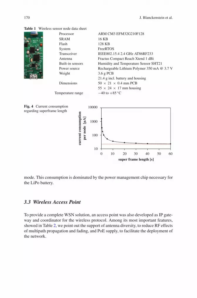
170 J. Blanckenstein et al.

Table 1 Wireless sensor node data sheetProcessor ARM CM3 EFM32G210F128SRAM 16 KBFlash 128 KBSystem FreeRTOSTransceiver IEEE802.15.4 2.4 GHz AT86RF233Antenna Fractus Compact Reach Xtend 1 dBiBuilt-in sensors Humidity and Temperature Sensor SHT21Power source Rechargeable Lithium Polymer 350 mA @ 3.7 VWeight 3.6 g PCB

21.4 g incl. battery and housingDimensions 50 × 21 × 0.4 mm PCB

55 × 24 × 17 mm housingTemperature range −40 to +85 ◦C

Fig. 4 Current consumptionregarding superframe length

10

100

1000

10000

0 10 20 30 40 50 60

curr

ent

cons

umpt

ion

per

node

[µ

A]

super frame length [s]

mode. This consumption is dominated by the power management chip necessary forthe LiPo battery.

3.3 Wireless Access Point

To provide a complete WSN solution, an access point was also developed as IP gate-way and coordinator for the wireless protocol. Among its most important features,showed in Table 2, we point out the support of antenna diversity, to reduce RF effectsof multipath propagation and fading, and PoE supply, to facilitate the deployment ofthe network.

A Scalable Redundant TDMA Protocol 171

Table 2 Wireless access point data sheetProcessor ARM926EJ

ARM CM3 EFM32GG330F1024SRAM 4 MB + 128 KBFLASH 8 MB + 1 MBSystem Embedded Linux + FreeRTOSTransceiver 2.4 GHz AT86RF233Antenna Dual diversity RP-SMA ConnectorPower source PoE (Power over Ethernet)Weight 47 g PCB

178 g incl. housing and antennasDimensions 76 × 63 × 1 mm PCB

94 × 134 × 46 mm housingTemperature range −40 to +85 ◦C

4 Results

First, the quality of the wireless channel is evaluated with respect to RSSI valuesand PER. Second, the impact of dual access points and different antenna selectionmodes is evaluated.

4.1 Base Measurements

The RSSI values obtained by the transceiver during the measurement campaignare in the range of −91 to −10 dBm with a resolution of 1 dBm and an accuracyof 3 dBm. In Fig. 5, the average RSSI value per node over the distance betweenthe access point and the corresponding node is shown, together with four aircraftchannel measurements from literature [12–15] and the free-space model. As can beseen, the RSSI values form a dense cloud around the channel measurements fromliterature. But in contrast to them, a trend line for the RSSI values would follow aneven steeper slope than suggested by the models. This is due to shadowing causedby real application positions, e.g. underneath the seats. Additionally, some nodes inplaces like the cargo compartment or the electronic bay have even lower RSSI valuesthan the majority of the nodes. These nodes form the scarce cloud below −70 dBm.Based on the measured distribution of the RSSI values we reason that a cell sizeof 10 m still leads to acceptable RSSI values. With a bigger cell radius the receivedsignal strength will decrease to a level where it will have significant impact on thepacket error rate for the current system.

Figure 6 shows the difference of averaged RSSI values per node; in Fig. 6a themean RSSI values of AP 1 are subtracted from AP 0 and in Fig. 6b the mean RSSIvalues of the downlink are subtracted from the uplink. The difference of the values

172 J. Blanckenstein et al.

Fig. 5 Average RSSI pernode compared to channelmeasurements from literature

-100-90-80-70-60-50-40-30-20-10

0

0 5 10 15 20 25 30R

SSI

[dB

m]

distance [m]

A330-300Free-spaceB777-200 [14]B767-300 [13]A340-300 [12]A319-100 [15]

can indicate if the channel is biased. In Fig. 6a, the RSSI values deviate around acommon mean (≈ −2.1 dB); the received signal strength for AP 1 is slightly higher.As outlined in Sect. 3.1 the nodes are not equally distributed throughout the aircraftand therefore the distance to Access Point 1 is a little bit shorter on average; hence thehigher RSSI values. Nevertheless, there are lots of nodes for which the signal strengthis higher at AP 0. This emphasizes the benefit of the multi-AP approach to utilizespatial diversity. In Fig. 6b the difference of the RSSI values of uplink−downlink isshown. The deviation of the difference is smaller than in Fig. 6a and in the regionof the accuracy of the RSSI values. We expected this deviation, but with a meanof 0 instead of −2.6 dB. The RSSI values for the downlink were always higherthan for the uplink. Most probably it is caused by non-reciprocal components in theaccess points, but this has to be validated with further measurements. Figure 7 showsthe packet error rate for all nodes in the uplink case. Figure 7a shows the uplinkpacket error rate with an abscissa scaling up to 1. As can be seen, for most of thenodes the PER is quite low with the exception of some outlier nodes. The moderateoutliers occur when the link quality is poor due to “challenging” placements of thenodes. The outliers with high values result from nodes which lost connectivity tothe APs for a long time. In Fig. 7b the abscissa is scaled up to a PER of 0.01 andoutliers above a threshold of 0.01 are removed to improve the visualization. As canbe seen, the packet error rate varies over the nodes, but the combined PER (greenarea) is always lower than the PER when just using AP 0 or AP 1. With two accesspoints per cell in the uplink case the combined PER is more than four times lowerthan compared to the PER when only using either AP 0 or AP 1. Because of thehigh PER of the outliers the mean is not a well suited measure for the tendency ofthe PER. When comparing the mean value for a = 1.1 · 10−2 (with outliers) withb = 4.9 · 10−4 (without outliers) the discrepancy is obvious. Instead, the median forboth cases equals 2.5 · 10−4 and is therefore used in the remainder of the chapter asthe measure for comparing PERs.

A Scalable Redundant TDMA Protocol 173

0 100 200 300 400 500−25

−20

−15

−10

−5

0

5

10

15

20

25

node IDs

mea

n R

SSI

AP

0 −

mea

n R

SSI

AP

1 [d

B]

differencemean

0 100 200 300 400 500−25

−20

−15

−10

−5

0

5

10

15

20

25

node IDs

mea

n R

SSI

uplin

k −

mea

n R

SSI do

wnl

ink

[dB

]

differencemean

(a) (b)

Fig. 6 a Difference of the mean RSSI values of AP 0 and 1, and b Difference of the mean RSSIvalues of uplink and downlink

0 100 200 300 400 5000

0.001

0.002

0.003

0.004

0.005

0.006

0.007

0.008

0.009

0.01

node IDs

PE

R

AP 0 AP 1 combinedmedian combined

0 100 200 300 400 5000

0.1

0.2

0.3

0.4

0.5

0.6

0.7

0.8

0.9

1

node IDs

PE

R

AP 1AP 0combined

(a) (b)

Fig. 7 a PER for the uplink, and b PER for the uplink with all outliers (above 0.01) removed

4.2 Impact of Dual Access Points

Two APs are responsible for each cell. Downlink packets—beacons included—aresent by both APs. Uplink packets are broadcast and because of the cell size canbe received by both APs. Therefore, in both directions spatial diversity and in thedownlink also temporal diversity is exploited.

To gain as much diversity as possible, the best case would be when the linksto AP 0 and AP 1 were statistically independent. Then, the combined PER wouldequal the product of the individual PERs of the APs, (PERC = PERAP0 · PERAP1).To evaluate the dependency of those links, we calculated the cross-correlation ofthe RSSI values and determined the Pearson product-moment correlation coefficientper node. A high correlation coefficient means that both APs measure similar RSSI

174 J. Blanckenstein et al.

−90 −80 −70 −60 −50 −40 −30

−90

−80

−70

−60

−50

−40

−30

RSSI [dBm] for AP 0

RSS

I [d

Bm

] fo

r A

P 1

ρ0,1 = 0.90

−90 −80 −70 −60 −50 −40 −30

−90

−80

−70

−60

−50

−40

−30

RSSI [dBm] for AP 0

RSS

I [d

Bm

] fo

r A

P 1

ρ0,1 = 0.04

(a) (b)

Fig. 8 Time-aligned RSSI values for AP 0 and 1 in the downlink; a RSSI values for node 165 (highcorrelation coefficient), and b RSSI values for node 45 (low correlation coefficient). The diameterof the circles is proportional to the number of measurements

values, while a low coefficient means that their measurements are independent fromeach other. Figure 8 visualizes this dependency with the help of two examples.The links for the depicted node in Fig. 8a are statistically dependent; both APsmeasure similar RSSI values at each time, which therefore form a cloud around thebisecting line. Statistically independent links are depicted in Fig. 8b. For this node,no correlation can be observed for the measured RSSI values. The values do notfollow the bisecting line, but they seem to be equally distributed. The links to bothAPs are slightly correlated, but this correlation is still low enough to exploit diversity.The mean correlation coefficient over all nodes in the downlink equals 0.30 with astandard deviation of 0.42, while for the uplink the mean equals 0.21 with a standarddeviation of 0.31. The high deviation indicates a different potential gain for eachnode by the multi-AP approach; nevertheless, for most of the nodes the impact willbe high. Figure 9 shows the median of the PERs for the downlink, the uplink, andfor the round-trip communication. The PER for AP 1 is in all three cases slightlyhigher than the PER for AP 0. In the downlink 18 %, in the uplink 9 %, and forthe round-trip 17 %, even though AP 1 received a 2.1 dB stronger signal. As can beseen in Fig. 5, the RSSI values are in the region of −40 to −70 dBm, therefore evenwith a 2.1 dB weaker signal the signal-to-noise ratio is still high and will have nobig influence on the PER. The same is valid when comparing the downlink with theuplink. The 2.6 dB stronger signal in the downlink also has no significant influence onthe PER.The combined PER will be lowest, if both links are statistically independent.With the given PERs for AP 0 and AP 1, this lower bound is in the order of 10−6. Themeasured combined PER was in the order of 10−4. Nevertheless, in all three cases thecombined PER is much lower than with only one AP, which clearly shows the benefitof the multi-AP approach when introducing spatial diversity. The round-trip PER isof course higher than only for the down- or uplink. Nevertheless, the combined PER

A Scalable Redundant TDMA Protocol 175

Fig. 9 Median of PER forAP 0, 1, and combined

DOWNLINK UPLINK ROUND−TRIP0

1E−04

5E−04

1E−03

2E−03

med

ian

of P

ER

s

AP 0AP 1combined

in the round-trip case is still lower than the PERs for AP 0 or 1 in down- and uplinkindividually.

4.3 Impact of Antenna Selection

As explained in Sect. 3.3 the access point is equipped with two antennas, where onlyone of them can be selected at a time. There are three different antenna selection(AS) modes available: AS 1 for always using the first antenna, AS 2 for always usingthe second antenna, and AS 3, the antenna auto-select mode, where the transceiverchooses the antenna. For more detail on auto-select mode, see Sect. 11.4 in the datasheet of the transceiver Atmel AT86RF233. We made sure that always the same ASmode was selected for all access points. To evaluate the impact of the AS modes inFig. 10a the median of the packet error rates for different antenna selection modesare depicted. The minimal resolution of the PERs is a consequence of the limitedmeasurement time. This minimal resolution is depicted as the black bar within eachPER bar. As can be seen, for mode AS 3 the measured PER is identical to theresolution of these measurements and therefore can only be used as the upper bound.The PER for the antenna selection mode AS 2 is always slightly higher than forAS 1. In Fig. 10b the ratio of the packet error rates for up- and downlink are shown.As can be seen, for all combinations the ratio is nearly one, which means that eachchosen antenna selection mode has the same impact on the PER even though thedownlink has a 2.6 dB higher RSSI than the uplink. It becomes obvious that themulti-AP approach has a much higher impact on the PER compared to the impact ofdifferent antenna selection modes. Because of the limited time for the measurementsthe impact of different antenna selection modes could not be investigated with therequired resolution. This will be done in future measurement campaigns.

176 J. Blanckenstein et al.

DOWNLINK UPLINK ROUND−TRIP0

2E−04

4E−04

6E−04

8E−04

1E−03

med

ian

of P

ER

s

AS 1AS 2AS 3

AS1 AS2 AS30

0.2

0.4

0.6

0.8

1

1.2

1.4

1.6

quot

ient

of

PER

s

median U/Dmean U/D

(a) (b)

Fig. 10 a Median PER for AS modes, and b Ratio of PER for up- and downlink

5 Conclusions

A wireless sensor network with 500 sensor nodes was successfully deployed in anAirbus A330–300. The designed TDMA protocol abstains from multihop and fromARQ-based retransmissions in order to provide guaranteed maximum delay whilemaintaining a high channel utilization. Robustness is achieved by spatial redundancyprovided by multiple APs. The measured environment is even more challenging thansuggested by channel models from literature, which becomes obvious when compar-ing the measured distribution of RSSI values with the models. The reason for thatis the deployment of the nodes at the application positions, e.g. in the life vest com-partments under the seats. Two APs per cell were used to introduce spatial diversity.This diversity reduced the PER significantly. The access points were equipped withtwo antennas, but the measurement results did not show significant impact on thePER when selecting one or the other.

A new measurement campaign will be conducted to evaluate the decrease ofPER when using more than two access points per cell and to find out when increas-ing spatial diversity stops improving PER. Additionally, the extended measurementcampaign will be used to gather more data. This is necessary to increase the resolu-tion of the PER and to be able to investigate the impact of antenna selection morethoroughly.

A Scalable Redundant TDMA Protocol 177

References

1. Lewandowski, A., Michaelis, S., Wietfeld, C., Klaue, J., Kubisch, M.: In-cabin localizationsolution for optimizing manufacturing and maintenance processes for civil aircrafts. In: PositionLocation and Navigation Symposium (PLANS), 2012 IEEE/ION, pp. 1257–1264 (2012)

2. Österlind, F., Dunkels, A.: Approaching the maximum 802.15.4 multi-hop throughput. In:Proceedings of the Fifth ACM Workshop on Embedded Networked Sensors (HotEmNets 2008),June 2008

3. Petrova, M., Riihijarvi, J., Mahonen, P., Labella, S.: Performance study of ieee 802.15.4 usingmeasurements and simulations. In: IEEE Wireless Communications and Networking Confer-ence, 2006, WCNC 2006, vol. 1, pp. 487–492 (2006)

4. Lee, T.-J., Lee, H.R., Chung, M.Y.: MAC throughput limit analysis of slotted CSMA/CA inIEEE 802.15.4 WPAN. IEEE Commun. Lett. 10(7), 561–563 (2006)

5. Suriyachai, P., Roedig, U., Scott, A.: A survey of MAC protocols for mission-critical applica-tions in wireless sensor networks. IEEE Commun. Surv. Tutorials 14(2), 240–264 (2012)

6. Suriyachai, P., Roedig, U., Scott, A.: Implementation of a MAC protocol for QoS supportin wireless sensor networks. In: IEEE International Conference on Pervasive Computing andCommunications, 2009, PerCom 2009, pp. 1–6 (2009)

7. Felemban, E., Lee, C.-G., Ekici, E.: MMSPEED: multipath multi-SPEED protocol for QoSguarantee of reliability and timeliness in wireless sensor networks. IEEE Trans. Mobile Comput.5, 738–754 (2006)

8. Munir, S., Lin, S., Hoque, E., Nirjon, S.M.S., Stankovic, J.A., Whitehouse, K.: Addressingburstiness for reliable communication and latency bound generation in wireless sensor net-works. In: Proceedings of the 9th ACM/IEEE International Conference on Information Process-ing in Sensor Networks, IPSN ’10, pp. 303–314. New York, USA (2010)

9. Suriyachai, P., Brown, J., Roedig, U.: Time-critical data delivery in wireless sensor networks.In: Proceedings of the 6th IEEE international conference on Distributed Computing in SensorSystems, DCOSS’10, pp. 216–229. Springer, Heidelberg (2010)

10. Chen, D., Nixon, M., Mok, A.: WirelessHART: Real-Time Mesh Network for IndustrialAutomation, 1st edn. Springer, NewYork (2010)

11. Kaouris, A., Zaras, M., Revithi, M., Moraitis, N., Constantinou, P.: Propagation measurementsinside a B737 aircraft for in-cabin wireless networks. In: IEEE Vehicular Technology Confer-ence 2008, VTC Spring 2008, pp. 2932–2936 (2008)

12. Moraitis, N., Constantinou, P.: Radio channel measurements and characterization inside air-crafts for in-cabin wireless networks. In: IEEE 68th Vehicular Technology Conference, 2008.VTC 2008-Fall, pp. 1–5 (2008)

13. Hankins, G., Vahala, L., Beggs, J.H.: Propagation prediction inside a B767 in the 2.4 GHz and5 GHz radio bands. In: IEEE Antennas and Propagation Society International Symposium,2005, vol. 1A, pp. 791–794 (2005)

14. Hankins, G., Vahala, L., Beggs, J.H.: 802.11ab propagation prediction inside a B777. In:IEEE/ACES International Conference on Wireless Communications and Applied Computa-tional Electromagnetics 2005, pp. 837–840 (2005)

15. D’Errico, R., Rudant, L.: UHF radio channel characterization for wireless sensor networkswithin an aircraft. In: Proceedings of the 5th European Conference on Antennas and Propagation(EUCAP), pp. 115–119 (2011)

Do We Really Need a Priori LinkQuality Estimation?

Vasilis Vasilopoulos, Daniele Puccinelli and Marco Zúñiga

Abstract Traditionally, link quality estimation (LQE) has been viewed as an a prioristep in sensor network routing protocols because it filters out unreliable links beforedata transmission. Recent results, however, show that protocols can perform wellwithout a priori LQE. Because getting rid of LQE seems rather counter-intuitive,the aim of this work is to look deeper into the behavior of LQE-free protocols. Ourresults, based on one of the state-of-the-art LQE-free protocols, show two interestinginsights. First, LQE-free protocols manage to choose links that are slightly betterthan the ones obtained with a priori LQE methods. Second, in traditional protocols,the effort needed to identify good links accounts, on average, for roughly half ofthe energy consumption of nodes, depending on the nodes’ active period and on theinter-packet interval. By eliminating this overhead, LQE-free protocols can save asignificant amount of energy compared to standard approaches.

1 Introduction

Traditional collection protocols in sensor networks, such as CTP [1] and Arbutus [2],employ a two-step approach to build their routing structure. First, nodes performlink quality estimation (LQE) to get a sense of all the possible usable links. Then,each node forms a routing path on top of these usable links (according to a givenmetric). Performing link quality estimation makes sense because unreliable linksare commonplace in sensor networks (due to the use of low-cost radios) and it isimportant to filter them out to increase reliability.

In the last couple of years, however, a new generation of collection protocols [3–6]have challenged this traditional view, and they have achieved better energy efficiency

V. Vasilopoulos · M. Zúñiga (B)

Delft University of Technology, Delft, The Netherlandse-mail: m.a.zunigazamalloa@tudelft.nl

D. PuccinelliUniversity of Applied Sciences and Arts of Southern Switzerland, Manno, Switzerland

K. Langendoen et al. (eds.), Real-World Wireless Sensor Networks, 179Lecture Notes in Electrical Engineering 281, DOI: 10.1007/978-3-319-03071-5_19,© Springer International Publishing Switzerland 2014

180 V. Vasilopoulos et al.

than CTP-like approaches. While all these new protocols have their own distinctivefeatures, they share a common characteristic: they do not perform a priori link qualityestimation. This observation motivated us to look deeper into the (in)significance oflink quality estimation for sensor networks.

The most important task of sensor networks is the ability to deliver data. Linkquality and path length play a central role in this respect: the better the link and theshorter the path, the higher the delivery rate. But, if no a priori link quality estimationis performed, several important questions arise. Without LQE, how good (or bad)are the selected links? What is the impact on the path length? The new generation ofcollection protocols reports delivery rates that are comparable or higher than CTP;therefore, they must be utilizing good links. Does this imply that a priori LQE is notnecessary?

Furthermore, since link quality estimation typically comes with a sizable controltraffic overhead and, therefore, a potentially significant energy footprint, it is impor-tant to quantify the exact energy demands of LQE methods (since the eliminationof these extra energy demands may be the core reason why the new generation ofprotocols outperform the older one).

In this chapter we report some preliminary results that are part of a wider researcheffort aiming at understanding LQE-free protocols. We selected the Broadcast-FreeCollection Protocol (BFC [6]) as an initial step to delve into the questions posedabove. Our empirical evaluation provides some interesting insights:

• LQE-free protocols choose links that are as good as, or even slightly better thanthose chosen by a priori LQE methods. While our results are based on BFC,we conjecture that this behavior also holds for other protocols (at least in somescenarios).

• We analyze the energy budget of CTP, dividing it between the parts used for controltraffic (mainly LQE) and data transmissions. Our results show that the control traf-fic part uses between 40 and 60 % of the energy resources of nodes (depending onthe nodes’ active period and on the inter-packet interval). Quantifying this over-head is central to understand the (in)efficiency of methods aiming at identifyinggood links.

2 Preliminaries

In recent years, several collection protocols have been proposed that do not rely onLQE as heavily as in previous research efforts, which treated it as an indispensablebuilding block. Before describing the related work in detail, it is important to highlightthat this new generation of LQE-free protocols provides the same delivery rate asCTP [1] and most of these new protocols do so by consuming less energy.

The summary of the state-of-the-art is captured in Table 1. For the duty cycle wedo not provide the actual numbers, but rather a relative metric (since most of thecorresponding chapters used different evaluation scenarios). For example, the value

Do We Really Need a Priori Link Quality Estimation? 181

Table 1 Performance of recent collection protocols

BCP LWB ORW BFC CTP

Relative duty cycle (%) >5 0.34 0.4 0.53 1Delivery rate (%) >97 >99 >99 >99 >99

of 0.4 for ORW indicates that the duty cycle of this protocol is on average 60 % lessthan in CTP (as reported by the authors).

2.1 Related Work

The Backpressure Collection Protocol (BCP) [3] employs a data-driven approachand forwards packets to the neighbor with the lowest queue level. It is a notableexample of structure-free routing, but it is not a great fit for duty-cycled sensornetworks because it requires a significant level of offered load to be effective, andthis increases the energy consumption of nodes (see Table 1).

The Low-Power Wireless Bus (LWB) [5] describes a way to perform datadissemination without utilizing LQE. LWB effectively turns a multi-hop low-powerwireless network into a shared bus, where all nodes are potential receivers of alldata. LWB leverages constructive interference to perform ultra-cheap and ultra-lightnetwork wide floods. The main limitation of this protocol with respect to CTP is thatit is centralized; one node in the network is responsible for synchronizing the fastfloods of all the other nodes.

The aforementioned protocols are great examples of new radical ways to dissem-inate and collect data without a priori LQE. Their mechanisms are, nevertheless,fundamentally different from CTP. BCP requires an artificially high offered load tobootstrap the system and LWB is centralized. To have a good (and fair) insight intothe benefits of LQE-free approaches, we believe that it is better to first use protocolsthat, in spirit, are closer to CTP. Below we describe two of such protocols.

In Opportunistic Routing in Wireless Sensor Networks (ORW) [4], the sink firstperforms floods to form a gradient centered around itself. The nodes then use oppor-tunistic unicast transmissions to forward data to the first neighbor that wakes up andthat provides progress towards the sink (i.e. a node with a higher gradient). ORWdoes not rely on a priori LQE methods except for one instance, when nodes cannot find a parent. The authors describe their approach as a “coarse-grained flavor ofLQE”.

The Broadcast-Free Collection protocol (BFC) [6] completely avoids LQE whilebuilding a data collection tree. BFC relies on eavesdropping nodes that already have apath towards the sink. The protocol is bootstrapped by the sink neighbors, which upontransmitting their first data packets get direct acks from the sink. The eavesdroppingprocess is repeated by nodes further down the tree until all nodes get a path. If a nodeis unable to eavesdrop on a potential parent, it remains disconnected until a potentialparent appears in its vicinity.

182 V. Vasilopoulos et al.

Selecting the best candidate for comparison As mentioned in Sect. 1, this chapterdescribes our first effort aiming at understanding LQE-free protocols. As a startingpoint we required a protocol that resembles CTP as much as possible but that requiresno a priori LQE. ORW and BFC are similar to CTP, but ORW still performs somelevel of LQE (albeit minimal). To avoid obtaining wrong insights, such as gettingLQE help from ORW when a node cannot find a parent, we decided to use BFC asa stepping stone.

Novelty This study is the first to identify that many of the newly proposed collectionprotocols have a common characteristic: the lack of LQE. Considering that we useBFC as a stepping stone to understand LQE-free protocols, it is important to highlighthow our work differs from the study presented by Puccinelli et al. [6]. In that work,the authors propose BFC, provide an analytical model for the duty cycle of differenttypes of nodes and compare BFC with CTP with respect to energy, delivery rate andlatency. Their evaluation results do not look into the routing structure (link qualityand path length) resulting from the lack of LQE methods. Also, while the authors doprovide a thorough evaluation of energy consumption, they do not compare it witha dissected energy budget from CTP, i.e. CTP control traffic separated from CTPdata traffic. This dissection is important because, as it will be explained later (seeSect. 3.4), it allows us to compare LQE-free protocols with the “LQE-free” version ofCTP (which is obtained if the period of the Trickle timer in CTP increases to infinity).What is more, the above-mentioned dissection allowed us to trace a bug in the BFCcode that was penalizing BFC’s energy performance substantially. Finally, while theauthors do mention that BFC may result in unbalanced networks, we provide datathat supports their hypothesis. Overall, our goal is to better understand the propertiesof LQE-free operations using BFC as a case study of LQE-free operation and CTPas a case study of LQE-based operation.

2.2 Evaluation Methodology

Our experimental evaluation is based on the Indriya testbed [7]. We selected thistestbed because it offers reasonably challenging testbed conditions as well as a rel-atively large-scale network (138 active nodes as of spring 2013).

We used existing TinyOS implementations of CTP and BFC, and ran bothprotocols on top of BoX-MAC [8]. In all of our experiments nodes inject one datapacket every 5 min (a reasonable interval value for several data collection applica-tions). The sink was located at one edge of the network (node 1 in the top right corner)and it was always on (a typical choice since the sink is normally connected to a stationwith unlimited access to energy resources). Given that sensor network testbeds canhave different connectivity patterns at different times [9], we always ran BFC andCTP back-to-back so that both protocols could operate under similar conditions. Weused a transmit power of 0 dBm on 802.15.4 channel 26 in all experiments.

Do We Really Need a Priori Link Quality Estimation? 183

Even though we ran experiments over several LPL wake-up interval values, in thischapter we show the results for a wake-up interval of 1 s because it is in the optimaloperating range of CTP—with respect to energy consumption—for the assumedoffered load of 1 packet per node every 5 min. For all the other LPL intervals (>1 s),BFC performed even better than CTP. In line with most experimental studies in thisarea, we use the duty cycle as a proxy for energy consumption [10].

In the next section, we report our results based on the different roles that nodesplay in the network. This is done because the sink neighbors, relays and leaves canhave vastly different performances. The sink neighbors are the nodes that can reachthe sink in one hop, relays are the nodes that are not sink neighbors but that needto forward packets for other nodes (besides their own packets), and leaves are thenodes that only have to send their own packets.

3 Experimental Study

Our evaluation has two overarching goals. First, to understand the impact of elimi-nating a priori LQE on the underlying routing structure (link quality and path length).Second, to quantify the impact of LQE methods on the network’s energy consumption(duty cycle and load balance). Overall, our evaluation captures four messages:

• LQE-free protocols seem to select links that are as good as those chosen by LQEmethods.

• The paths of LQE-free protocols tend to be longer than those found in LQE-basedprotocols.

• By eliminating LQE, protocols can save a substantial amount of energy. For LPLwake-up interval of 1 s and inter-packet interval of 5 min, this translates into areduction of energy expenses between 40 and 60 %.

• Depending on the method, LQE-free protocols may lead to a better or worse loadbalance. In the case of BFC, the load balance and, therefore, the energy balanceis worse.

3.1 Link Quality

To utilize a common metric, we define link quality as the average number oftransmissions required to send successfully a packet from any node to its imme-diate parent. Figures 1 and 2 show the cumulative distribution function (cdf ) forall child-parent links for relay and leaf nodes, respectively, and Table 2 reports themean and standard deviation. We observe that performing a priori LQE does nothelp in selecting better links. In fact, BFC tends to select better links. CTP’s linksare roughly 9 % costlier than BFC’s for relays and 5.5 % costlier for leaves on thisoccasion. Below we provide a conjecture as to why this happens. We do not showthe results for the sink neighbors because all of these nodes had perfect links withCTP and BFC.

184 V. Vasilopoulos et al.

Fig. 1 CDF of the averagenumber of transmissions to theselected parent for the relays

0 1 2 3 40

0.2

0.4

0.6

0.8

1

Em

piric

al C

DF

Transmission Count to Parent

BFC

CTP

Fig. 2 CDF of the averagenumber of transmissions to theselected parent for the leaves

0 1 2 3 40

0.2

0.4

0.6

0.8

1

Em

piric

al C

DF

Transmission Count to Parent

BFC

CTP

Table 2 Link quality (# transmissions)

Relays LeavesCTP BFC CTP BFC

Average (μ) 1.15 1.05 1.27 1.20Std dev (σ ) 0.14 0.11 0.42 0.36

Why does a priori LQE not seem to matter? The key limitation of LQE methodsis the presence of “intermittent” links. Based on the various LQE studies in theliterature [11], let us assume the following simplified classification of sensor networkslinks: (i) good, when they rarely drop a packet (very high signal-to-noise ratio, wayabove the radio sensitivity), (ii) intermittent, when they have periods of good qualitybut also periods of bad quality (the signal-to-noise ratio oscillates around the radio

Do We Really Need a Priori Link Quality Estimation? 185

sensitivity), (iii) unreliable, when most of the time their quality is below good (thesignal-to-noise ratio is usually below the radio sensitivity). LQE methods are verygood at discarding unreliable links, but not so good at discarding intermittent links(because there is a chance that the quality is measured during a good period). Infact, Alizai et al. identified this limitation as a weakness of CTP but from a differentperspective [12]. That study claimed that CTP was too conservative. By discardingsome of these intermittent links, CTP was not taking advantage of those links’ goodperiods, which decreased its performance. In this study, we move in a differentdirection. We conjecture that LQE-free protocols overcome the lack of LQE methodsby being even more conservative on the utilization of intermittent links.

In BFC, nodes have a pre-determined parent (as in CTP), but the network reliessolely on good links. In BFC, a node is considered a parent if three consecutivedata packets arrive from the (potential) child node. Notice that BFC does not use asingle beacon to find a parent, BFC simply relies on sniffing and latching on nodesthat already found a path towards the sink. Given that (i) in most data collectionapplications the period between consecutive data packets is of a few minutes, andthat (ii) intermittent links are bursty in nature [11]; by validating a link every fewminutes, the chances of picking an intermittent link are significantly reduced. BFC isconservative in the sense that, by default, its data path validation mechanisms discardunreliable and intermittent links. This conservative approach, letting BFC assumesymmetric links, may explain why BFC selects slightly better links than CTP.

In ORW [4], nodes do not have a pre-determined parent; they transmit informationopportunistically using a unicast paradigm. In this way, nodes do not assume that alink exists (which is what protocols with a priori LQE methods do); a node uses whatis available at the moment. Given that link quality is known to be highly correlatedin time, ORW usually ends up selecting either good links or intermittent links duringgood periods. ORW is conservative in the sense that unless a link is currently good,it assumes that it does not exist.

3.2 Path Length

In CTP, the a priori LQE phase not only allows the network to identify good links,but this preliminary information is also used to identify short paths. On the otherhand, in LQE-free protocols nodes do not have this extra information, and hence,they may end up using longer routes. Figures 3 and 4 show the cdf of path lengths forrelays and leaves, and Table 3 reports the mean and standard deviation. The absenceof LQE clearly affects the depth of the data collection tree. Thanks to LQE, CTP’sroutes are roughly 8 % shorter for relays and 13 % shorter for leaves on this occasion.Even though we did not perform experiments with ORW, we expect this trend to bethe same. Due to the opportunistic nature of ORW transmissions, packets can followpaths that deviate significantly from the shorter routes identified by CTP.

186 V. Vasilopoulos et al.

Fig. 3 CDF of the averagenumber of hops to the sink forthe relays

1 2 3 4 5 6 70

0.2

0.4

0.6

0.8

1

Em

piric

al C

DF

Path Length

BFC

CTP

Fig. 4 CDF of the averagenumber of hops to the sink forthe leaves

1 2 3 4 5 6 70

0.2

0.4

0.6

0.8

1

Em

piric

al C

DF

Path Length

BFC

CTP

Table 3 Path length (# hops)

Relays LeavesCTP BFC CTP BFC

Average (μ) 2.72 2.95 3.36 3.85Std dev (σ ) 0.77 0.80 0.99 0.87

3.3 Link Quality Versus Path Length

Link quality and path length are jointly responsible for the formation of the datagathering tree, i.e. building the routing structure. To provide a comprehensive viewof the relation between link quality and path length, Figs. 5 and 6 show the routingcost (number of transmissions required to deliver a packet to the sink) versus the

Do We Really Need a Priori Link Quality Estimation? 187

Fig. 5 Routing cost versuspath length for the relays

1 2 3 4 5 61

2

3

4

5

6

7

8

Path Length

Rou

ting

Cos

tBFC

CTP

Fig. 6 Routing cost versuspath length for the leaves

1 2 3 4 5 61

2

3

4

5

6

7

8

Path Length

Rou

ting

Cos

t

BFC

CTP

path length for relays and leaves. If all paths were error-free, the plot would show aline with slope 1. At first glance, we could state that LQE-methods are more efficientbecause they provide shorter paths with similar link qualities, that is, they requireless transmissions to deliver the same amount of data. But as we will observe next,these savings are minimal compared to the energy expenses of CTP control traffic(which is required to find these good short routes in the first place).

3.4 Energy Efficiency

We have seen that without employing LQE underneath, BFC still opts for good links.Now, we will proceed to understand why the overall operation of BFC, and LQE-free

188 V. Vasilopoulos et al.

Fig. 7 Mean duty cycle forsink neighbors, relays andleaves

sink neighbors relays leaves0

0.5

1

1.5

2

Mea

n D

uty

Cyc

le (

%)

CTP DataCTP ControlBFC

protocols in general, can be so energy-efficient. To this end, we changed slightly theCTP code to monitor the fractions of the duty cycle related to control traffic andto data traffic. We also found a bug in the BFC code that penalized its duty cycle(i.e. BFC’s energy performance is better than the measurements reported in [6]).Figures 7 and 8 show the mean and median duty cycle for the three types of nodes.The median plot allows us to filter out connectivity outliers.

Figure 8 shows that the cost of CTP control traffic is similar for all node classes,in the order of 0.5 %. This occurs because CTP periodically sends probes to testthe connectivity of nodes. It is important to highlight that these measurements wereperformed once CTP and BFC reached a stable state, that is, after the initial probingrequired to bootstrap the network (otherwise the duty cycle of CTP would be evenhigher). The important lesson from this result is that it gives us an “LQE-free”version of CTP (captured by the white bars). Assuming an ideal static environment,CTP would need to run the Trickle timer only once (at the beginning). Then, afterthe routes are formed, the LQE phase would not need to be run again because linkswould not change. This result allows us to benchmark an LQE-free protocol, suchas BFC, with an ideal “LQE-free” version of CTP.

It is important to note that BFC has some other disadvantages besides the longlatency mentioned in [6]. A priori LQE also allows a better responsiveness. CTPwould react much faster to changes in the environment than BFC. For instance, ifa malicious interfering node is first turned on and then off. CTP would be able torapidly (re)identify the shorter paths “erased” by the interfering node. On the otherhand, BFC, would not be able to recover (or at least not fast enough) because noperiodic LQE measurements are done. As part of our future work, we plan to use theJamLab tool [13] to stress LQE-free protocols under different interference patterns.

Do We Really Need a Priori Link Quality Estimation? 189

Fig. 8 Median duty cyclefor sink neighbors, relays andleaves

sink neighbors relays leaves0

0.5

1

1.5

2

Med

ian

Dut

y C

ycle

(%

)

CTP DataCTP ControlBFC

3.5 Load Balancing

In [6], the authors mention that BFC seemed to have a worse load balance than CTP.We validate this hypothesis. Figures 9 and 10 illustrate the cdf of the forwardingload for the sink neighbors and relays. The forwarding load is defined as the ratio ofthe total number of forwarded packets (which includes locally generated and relayedpackets) per locally generated packet. We do not present the cdf for the leaves becausethe vast majority of them had a forwarding load of 1. Strictly speaking, all the leavesshould have a forwarding load of 1, but, in a real network, leaves may occasionallyact as relays for short periods of time. We, therefore, use a threshold of 2 to filter outsuch nodes from the set of real relays.

Fig. 9 CDF of the forwardingload for the sink neighbors

0 10 20 30 40 500

0.2

0.4

0.6

0.8

1

Em

piric

al C

DF

Forwarding Load

BFC

CTP

190 V. Vasilopoulos et al.

Fig. 10 CDF of the forward-ing load for the relays

0 10 20 30 40 500

0.2

0.4

0.6

0.8

1

Em

piric

al C

DF

Forwarding Load

BFC

CTP

Table 4 Jain’s fairness index

# Sink neighbors Index # Relays Index # Leaves Index

CTP 17 0.44 27 0.66 92 0.95BFC 22 0.18 21 0.44 93 0.96

Recalling that neither CTP nor BFC employ an explicit load balancing scheme,we see that BFC performs clearly worse than CTP with respect to sink neighbors (seeFig. 9). A few sink neighbors in BFC are responsible for forwarding 80 % of the load.The load balancing is better for the relays (see Fig. 10). To quantify the unfair shareof the forwarding load and consequently of the energy resources, we compute theJain’s fairness index for both CTP and BFC for all node classes in Table 4. A Jain’sindex of 1 denotes perfect balance (best-case value), while 1/n (where n denotes thenumber of nodes) indicates clear unfairness (worst-case value). If we consider allnodes, the Jain’s fairness index is 0.29 for CTP and 0.18 for BFC.

The reason for the worse load balance in LQE-free approaches seems to be thesame as for the longer paths (see Sect. 3.2). Without a priori LQE, a network not onlylooses the ability to identify good links but also to have a broader view of the under-lying communication graph. This broader view could facilitate the identification ofshorter paths and better load balancing.

3.6 Energy Efficiency Versus Load Balancing

To provide a complete view of the effect of LQE on the energy consumption ofindividual nodes, Figs. 11 and 12 show the duty cycle versus the forwarding load forthe sink neighbors and relays. Leaves can be regarded as relays that are responsible

Do We Really Need a Priori Link Quality Estimation? 191

Fig. 11 Duty cycle versusforwarding load for the sinkneighbors

0 5 10 15 20 25 30 35 400

1

2

3

4

5

6

Forwarding Load

Dut

y C

ycle

(%

)

BFC

CTP Data

CTP Total

Fig. 12 Duty cycle versusforwarding load for the relaysand the leaves

0 5 10 15 20 25 30 35 400

1

2

3

4

5

6

Forwarding Load

Dut

y C

ycle

(%

)

BFC

CTP Data

CTP Total

for forwarding only their own load (normally). Therefore, Fig. 12 depicts both nodeclasses jointly. We observe that, in general, BFC penalizes some individual nodes.As hypothesized in [6], this may be due to a “rich gets richer effect”. Nodes that arepicked first as parents are eavesdropped first, which in turn increases their number ofchildren and their forwarding load. This load balancing problem is not an intrinsicproblem of LQE-free protocols. We believe that the opportunistic nature of ORWwill naturally balance the load in the network because it can choose vastly differentpaths at each time (due to the presence of intermittent links). Analyzing the loadbalancing properties of ORW (among its many other LQE-free characteristics) ispart of our future work.

192 V. Vasilopoulos et al.

4 Conclusions

Our evaluation indicates that LQE might have been overrated. Not using LQE resultsin longer routes with extra hops, but it also results in more conservative routingdecisions, i.e. choosing individual links with a lower cost. The path length inefficiencycaused by the lack of LQE is therefore amortized at the root; on top of that, noLQE means no control overhead, which translates into a reduction of the energyfootprint of collection protocols between 40 and 60 % (for LPL wake-up intervalof 1 s and inter-packet interval of 5 min). Lack of fairness posed by load imbalanceis a clear drawback of LQE-free operation, though it can be avoided by abstractingaway from the network topology and getting every node to receive every packet asin [5]. Our results, however, clearly show that load imbalance does not have sizableconsequences in terms of energy consumption.

Acknowledgments We wish to thank our shepherd, Jason Gu, the anonymous reviewers, and themaintainers of publicly available testbeds. We gratefully acknowledge the TinyOS community andin particular all those researchers that have made their implementations available.

References

1. Gnawali, O., Fonseca, R., Jamieson, K., Moss, D., Levis, P.: Collection tree protocol. In:Proceedings of the 7th ACM Conference on Embedded Networked Sensor Systems, pp. 1–14.ACM, New York (2009)

2. Puccinelli, D., Haenggi, M.: Reliable data delivery in large-scale low-power sensor networks.ACM Trans. Sens. Netw. (TOSN) 6(4), 28:1–28:41 (2010)

3. Moeller, S., Sridharan, A., Krishnamachari, B., Gnawali, O.: Routing without routes: The back-pressure collection protocol. In: Proceedings of the 9th ACM/IEEE International Conferenceon Information Processing in Sensor Networks, pp. 279–290. ACM, New York (2010)

4. Landsiedel, O., Ghadimi, E., Duquennoy, S., Johansson, M.: Low power, low delay: opportunis-tic routing meets duty cycling. In: Proceedings of the 11th ACM/IEEE International Conferenceon Information Processing in Sensor Networks, pp. 185–196. ACM, New York (2012)

5. Ferrari, F., Zimmerling, M., Mottola, L., Thiele, L.: Low-power wireless bus. In: Proceedingsof the 10th ACM Conference on Embedded Networked Sensor Systems, pp. 1–14. ACM, NewYork (2012)

6. Puccinelli, D., Zúñiga, M., Giordano, S., Marrón, P.J.: Broadcast-free collection protocol. In:Proceedings of the 10th ACM Conference on Embedded Networked Sensor Systems, pp. 29–42. ACM, New York (2012)

7. Doddavenkatappa, M., Chan, M.C., Ananda, A.L.: Indriya: a low-cost, 3d wireless sensornetwork testbed. In: Testbeds and Research Infrastructure. Development of Networks andCommunities. Springer pp. 302–316 (2012)

8. Moss, D., Levis, P.: BoX-MACs: Exploiting Physical and Link Layer Boundaries in Low-PowerNetworking. Technical Report SING-08-00, Stanford University (2008)

9. Puccinelli, D., Gnawali, O., Yoon, S., Santini, S., Colesanti, U., Giordano, S., Guibas, L.: Theimpact of network topology on collection performance. In: Wireless Sensor Networks, pp.17–32. Springer, Heidelberg (2011)

10. Dunkels, A., Osterlind, F., Tsiftes, N., He, Z.: Software-based on-line energy estimation forsensor nodes. In: Proceedings of the 4th Workshop on Embedded Networked Sensors, pp.28–32. ACM, New York (2007)

Do We Really Need a Priori Link Quality Estimation? 193

11. Baccour, N., Koubaa, A., Mottola, L., Zúñiga, M.A., Youssef, H., Boano, C.A., Alves, M.:Radio link quality estimation in wireless sensor networks: a survey. ACM Trans. Sens. Netw.(TOSN) 8(4), 34:1–34:33 (2012)

12. Alizai, M.H., Landsiedel, O., Link, J.Á.B., Götz, S., Wehrle, K.: Bursty traffic over burstylinks. In: Proceedings of the 7th ACM Conference on Embedded Networked Sensor Systems,pp. 71–84. ACM, New York (2009)

13. Boano, C.A., Voigt, T., Noda, C., Römer, K., Zúñiga, M.: JamLab: Augmenting sensornettestbeds with realistic and controlled interference generation. In: Proceedings of the 10th IEEEInternational Conference on Information Processing in Sensor Networks, pp. 175–186 (2011)

Redundant Border Routersfor Mission-Critical 6LoWPAN Networks

Laurent Deru, Sébastien Dawans, Mathieu Ocaña, Bruno Quoitinand Olivier Bonaventure

Abstract Sensor networks are gradually moving towards full-IPv6 architecturesand play an important role in the upcoming Internet of Things. Some mission-criticalapplications of sensor networks will require a level of reliability that excludes thepresence of single points of failure, as it is often the case today for the gateways con-necting sensor networks to the Internet. In this chapter, we introduce RPL-6LBR, a6LoWPAN border router that addresses mission-critical deployments through redun-dancy. The chapter discusses how existing standards may be leveraged to enableredundant border router synchronization, while identifying certain of their short-comings. We also propose innovative network architectures incorporating multipleborder routers, which deal with redundancy and node mobility without requiring anysynchronization among the border routers. We implement the proposed RPL-6LBRin the Contiki operating system and report on this implementation through trialson a small-scale testbed and simulator. Our results open new possibilities for real-world wireless sensor networks requiring reliable border routers, and guide furtherstandardization efforts in emerging technologies in support of the Internet of Things.

L. Deru · S. Dawans(B) · M. OcañaCETIC, Rue des Frères Wright 29/3, B-6041 Charleroi, Belgiume-mail: sebastien.dawans@cetic.be

L. Derue-mail: laurent.deru@cetic.be

M. Ocañae-mail: mathieu.ocana@cetic.be

B. QuoitinUniversité de Mons, 20, place du Parc, B-7000 Mons, Belgiume-mail: bruno.quoitin@umons.ac.be

O. BonaventureUniversité Catholique de Louvain, B-1348 Louvain-la-Neuve, Belgiume-mail: olivier.bonaventure@uclouvain.be

K. Langendoen et al. (eds.), Real-World Wireless Sensor Networks, 195Lecture Notes in Electrical Engineering 281, DOI: 10.1007/978-3-319-03071-5_20,© Springer International Publishing Switzerland 2014

196 L. Deru et al.

1 Introduction

In the foreseeable future, billions of low power wireless devices will be connectedto the Internet. To make this Internet of Things (IoT) vision a reality, constraineddevices are adopting standards-based solutions [1]. The IoT embraces the IPv6networking architecture to fulfill these requirements. IPv6-based Wireless SensorNetworks (WSN) enable a diverse range of application domains from smart cities tobuilding and home automation. As the IoT-enabling technologies mature, so do therequirements on interconnectivity, reliability and fault-tolerance.

A key element of any deployed IoT network is the border router (BR) that connectsit to the Internet. The BR is a gateway between two different link-layer technologies,typically 802.15.4 on the WSN side, and Ethernet or Wi-Fi on the other. The BRalso separates the control planes of two different routing domains. In the majority ofcurrent deployments, the BR is unique.

When deploying large IoT networks, several issues appear such as the highsolicitation of nodes close to the BR, the single point of failure (SPoF) that theBR is, and interconnecting seamlessly with existing IPv6 networks. We argue thatfor reliable mission-critical networks, redundant BRs need to be deployed. With mul-tiple BRs, the packets can be load-balanced across these BRs and their neighboringnodes if the BRs are deployed at different physical locations, spreading the energyconsumption across the network and reducing the likelihood of bottlenecks duringtraffic bursts. Using multiple BRs also reduces the risk of unreachability of nodes ifnetwork partitioning occurs due to failures within the WSN. However, using multipleBRs raises new problems such as the need to synchronize them, how to recover fromfailures, how to handle node mobility and how to integrate them seamlessly into anexisting IPv6 network.

In this chapter, we analyze how large IoT networks attached via redundant BRs canbe deployed. Our work focuses on 6LoWPAN networks running RPL, the RoutingProtocol for Low-Power and Lossy Networks (LLNs), as it is the primary routingprotocol for IPv6 LLNs [2]. We analyze in detail how RPL networks support multipleBRs both in theory and in practice. We design a RPL 6LoWPAN Border Router (RPL-6LBR) solution supporting multiple BRs with node mobility and fault-tolerancewithout compromising the energy-efficient control mechanisms provided by RPL.Finally, we implement RPL-6LBR in the Contiki operating system and evaluate itsperformance.

2 Background

6LoWPAN and IPv6 operate on link layers that are fundamentally different: IPv6link layers such as Ethernet are highly-available, provide high throughputs with lowlatencies and are more reliable than LLNs. As a consequence, control-plane protocolsfor IPv6 and 6LoWPAN networks do not share the same constraints. In this section,

Redundant Border Routers for Mission-Critical 6LoWPAN Networks 197

we describe how RPL allows for low-overhead networking in support of LLNs, andwe further discuss how existing standards propose to interconnect IPv6 networksand 6LoWPAN.

2.1 RPL-based 6LoWPAN Networks

The Routing Protocol for LLNs (RPL) is a distance-vector routing protocol addressingthe problem of scalable any-to-any routing in low-power IPv6 networks [2]. RPLroutes upwards and downwards along a tree-like topology called Destination-Oriented Directed Acyclic Graph (DODAG), maintained via an adaptive beaconingmechanism. RPL provides good scalability with the network size because all thecontrol traffic is focused in optimizing a single topology towards a single destina-tion, rather than one route between all pairs of nodes in the network. It also favorsdata-driven link estimations, meaning it will not proactively waste energy attemptingto optimize its DODAG unless data packets are routed, which is attractive in termsof power savings. The main innovation of RPL is that it brings bidirectional trafficpatterns over lossy, multihop networks.

2.2 Interconnecting LLNs with IPv6

Figure 1 represents a typical network architecture integrating 6LoWPAN and IPv6networks. The BR may act as a router and separate the IPv6 and 6LoWPAN networksin different subnets, or act as a bridge, handling both IPv6 and 6LoWPAN networksas a common subnet.

These architectures support end-to-end IP communication between any host anda sensor on the LLN. To achieve this goal, 6LoWPAN transmits IPv6 packetsover IEEE 802.15.4 frames by adding an adaptation layer for header compressionand fragmentation [3]. For IPv6 control plane mechanisms, like the Neighbor

EthernetSwitch

InternetRouter

LAN Host Border Router

WSNaaaa::xxxx

BR as Bridgeaaaa::101

6LoWPANaaaa::1000

BR as Routerbbbb::101

BR as Bridgeaaaa::100BR as Routerbbbb::100

Internet

BR as Bridgeaaaa::1BR as Routerbbbb::1

Fig. 1 Border Router in a typical IPv6-6LoWPAN environment

198 L. Deru et al.

Discovery Protocol (NDP) [4], to operate on energy constrained and asymmet-ric networks, the IETF proposes the Neighbor Discovery Optimization for LLNs(6LoWPAN-ND) [5].

6LoWPAN-ND aims to support both proposed approaches to routing in 6LoW-PAN networks: route-over and mesh-under modes. However, 6LoWPAN-ND doesnot fully encompass the problem of interconnecting 6LoWPAN-based WSNs to theInternet, only interconnection by routing is explored.

To allow transparent communication as if the LLN is part of the IPv6 subnet,the Neighbor Discovery Proxy Gateway for 6LoWPAN-based WSNs (6LP-GW)provides bridging capabilities and allows an external host to discover and connectto sensors using NDP and protocol conversion between NDP and 6LoWPAN-ND[6]. However, that proposal does not cover the 6LoWPAN route-over scenario andits interaction with RPL.

2.3 Dealing with Mobility and Redundancy

Dynamic routing protocols like RPL are designed to adapt their routing strategiesagainst varying channel conditions. As a side effect, an immobile sensor can appear tobe mobile. RPL has built-in mechanisms to support inter-LoWPAN mobility thanks tothe multi-instance support and the capability to switch from one DODAG to anotherin the same instance.

6LoWPAN-ND does not have any requirement on inter-LoWPAN mobility inroute-over networks or on multi-BR support. This is out of scope of [5]. However,[5] requires that either sensors register their address towards all of the known 6LBRsor that an out-of-scope mechanism synchronize those 6LBRs. Again, no current6LoWPAN-ND implementation proposes any synchronization mechanisms. Thus,inter-LoWPAN mobility and redundancy is severely constrained as a WSN nodemoving from one DODAG to another will see the subnet prefix changing and thereforewill get a new global address. If each LLN is configured with its own prefix, MobileIPv6 or one of its variants could be implemented [7].

3 Design of a RPL-Compatible 6LBR

In order to tackle the shortcomings identified in the previous sections, we propose todefine the routing and mobility requirements for multi-BR RPL-based networks asfollows:

1. The BR must be compatible with RPL in a route-over mode.2. Multiple BRs must be able to co-exist in the same infrastructure, handling

contiguous or disjoint LLNs.3. Only one BR at a time should be responsible for a given 6LoWPAN host.

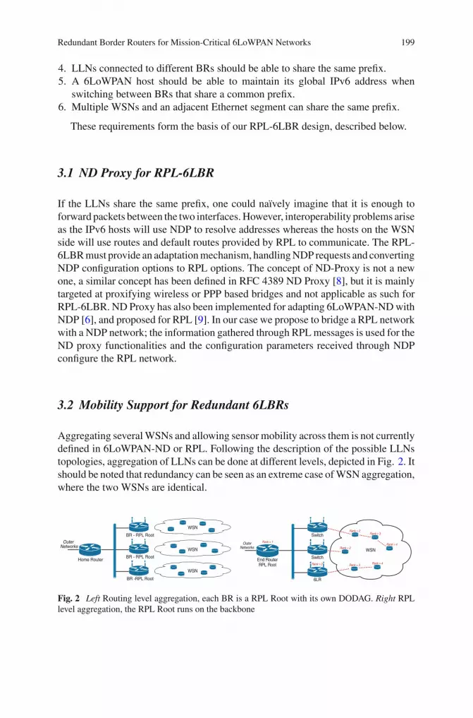
Redundant Border Routers for Mission-Critical 6LoWPAN Networks 199

4. LLNs connected to different BRs should be able to share the same prefix.5. A 6LoWPAN host should be able to maintain its global IPv6 address when

switching between BRs that share a common prefix.6. Multiple WSNs and an adjacent Ethernet segment can share the same prefix.

These requirements form the basis of our RPL-6LBR design, described below.

3.1 ND Proxy for RPL-6LBR

If the LLNs share the same prefix, one could naïvely imagine that it is enough toforward packets between the two interfaces. However, interoperability problems ariseas the IPv6 hosts will use NDP to resolve addresses whereas the hosts on the WSNside will use routes and default routes provided by RPL to communicate. The RPL-6LBR must provide an adaptation mechanism, handling NDP requests and convertingNDP configuration options to RPL options. The concept of ND-Proxy is not a newone, a similar concept has been defined in RFC 4389 ND Proxy [8], but it is mainlytargeted at proxifying wireless or PPP based bridges and not applicable as such forRPL-6LBR. ND Proxy has also been implemented for adapting 6LoWPAN-ND withNDP [6], and proposed for RPL [9]. In our case we propose to bridge a RPL networkwith a NDP network; the information gathered through RPL messages is used for theND proxy functionalities and the configuration parameters received through NDPconfigure the RPL network.

3.2 Mobility Support for Redundant 6LBRs

Aggregating several WSNs and allowing sensor mobility across them is not currentlydefined in 6LoWPAN-ND or RPL. Following the description of the possible LLNstopologies, aggregation of LLNs can be done at different levels, depicted in Fig. 2. Itshould be noted that redundancy can be seen as an extreme case of WSN aggregation,where the two WSNs are identical.

WSN

Outer Networks

Home Router

BR - RPL Root

BR - RPL Root

BR -RPL Root

WSN

WSN

WSN

Outer Networks

End Router RPL Root

Switch

Switch

6LR

Rank = 1

Rank = 2

Rank = 2

Rank = 2

Rank = 3

Rank = 3

Rank = 4

Rank = 4

Fig. 2 Left Routing level aggregation, each BR is a RPL Root with its own DODAG. Right RPLlevel aggregation, the RPL Root runs on the backbone

200 L. Deru et al.

Aggregating WSNs by synchronizing RPL-6LBR Aggregating WSNs usingND Proxy based RPL-6LBR sharing the same prefix is feasible but requires thesynchronization of the different RPL-6LBRs to allow sensor mobility. Otherwise,several RPL-6LBRs would perform ND Proxy for the same WSN node, which isundesirable. In this chapter we rely on the Neighbor Advertisements to synchronizethe ND Proxies of the connected RPL-6LBR.

Aggregating WSN using an external DODAG root RPL integrates sensormobility deeply, so an innovative solution we propose is to create a unique DODAGacross multiple BRs encompassing all the WSN nodes. This unique DODAG ismanaged by an External DODAG Root connected to the BRs through an Ethernetbackbone.

4 Implementation

We provide an implementation of our RPL-6LBR in the latest development version ofthe Contiki operating system.1 We support multiple types of RPL-6LBR platforms:the RapsberryPi with a custom 802.15.4 radio, the BeagleBone, the Econotag runningContiki natively and a standard Linux PC.

To enable multiple BR support in Contiki, we implement an ND Proxy as designedin Sect. 3.1 to adapt IPv6/NDP and 6LoWPAN/RPL. We also implement prefix distri-bution by leveraging the Prefix Information Option (PIO) of the RPL DIO broadcastmessages combined with a global reset of the DIO Trickle timer. Due to space limi-tations we refer the reader to the online documentation for implementation details.

5 Evaluation

We evaluate RPL-6LBR in different scenarios with a Python-based unit testframework, provided as part of the RPL-6LBR open-source repository.

As our implementation targets real deployments, the results in this chapter arepartially made up of tests on the RaspberryPi, interfaced with real sensor nodes ofour testbed: 20 nodes spread over a 500 m2 office space (10 TelosB, 10 Zolertia Z1).In order to explore certain parameters in a controlled manner, we also parallelizeda large number of test instances on Linux virtual machines, interfacing the sameRPL-6LBR with a virtual WSN using the COOJA simulator with TelosB emulatedsensor devices.

All sensor modules run a Contiki application over the ContikiRPL implementationusing the most commonly used configuration: the Minimum Rank Hop ObjectiveFunction (MRHOF) with ETX [10] as the routing metric and with RPL’s storingmode for downwards routing. We control the network size, topology, RPL DAGstabilization times and types and amount of cross-traffic. All runs consist in analyzing

1 http://cetic.github.com/6lbr. tag 6blr-1.1.0. 2013 (licence: BSD).

Redundant Border Routers for Mission-Critical 6LoWPAN Networks 201

Fig. 3 Time of propagation of new prefix versus hop count

the effects of cross-traffic, node mobility and prefix reconfiguration on bidirectionalapplication traffic between a host on the Ethernet network and a constituant of theWSN network, as far down the RPL DAG as possible. Each testcase was executed10 times, with different random seeds for the simulated ones.

Prefix distribution We measure the lapse of time during which a particular hoston the WSN is unreachable on a new prefix while this prefix is propagated on arunning network. Figure 3 shows the average duration of unreachability versus thedistance from the RPL Root for different traffic patterns. The main result is thatthere is little effect of the cross-traffic, prefix distribution being only dependant ofthe beaconing mechanisms of RPL.

Inter-WSN routing We next evaluate inter-WSN routing between two RPL-6LBRs set up in both SmartBridge and Switch modes, handling physically disjointWSNs. Ping messages are exchanged between elements of disjoint DODAGs (garan-teed in simulation), each roughly three hops away from its root. In SmartBridge mode,the Round Trip Times (RTT) of pings average 0.62 s± 0.12 s, which is slightly shorterthan the ones in the Switch mode measured as 0.67 s ± 0.12 s due to the extra hopthat is induced in Switch mode.

Node mobility On Fig. 4, we observe the behavior of RPL-6LBR in the presenceof a mobile node switching between DODAGs. We see that the performance isdependant of RPL’s link metric estimation. High data collection rates update themobile node’s ETX rapidly enough to allow it to select a member of the secondaryDODAG as preferred parent in all cases. On the other hand, low data collection ratesdo not all result in the reachability of the node within a 600 s limit we imposed, andthe trials that do converge exhibit a longer convergence time on average.

Border router outages In the case of BR outages, the effects of data-traffic isamplified (Fig. 5). A BR failure orphans the entire sub-DODAG originally handledby the BR and requires nodes closest to the alternate DODAG to update their linkETX first, then join the DODAG and announce their ranks to neighboring orphans viaDIOs. The remaining orphans of the previous DODAG gradually attach themselvesto the new DODAG in a hop by hop manner.

202 L. Deru et al.

Fig. 4 Mobile node trials. The success rate and unreachability duration is independent of whetheror not the other nodes of the network update their link metrics with periodic unicasts

Fig. 5 BR outage trials. The success rate and unreachability delay are improved when all elementsof the network accelerate their ETX updates as they emit periodic UDP messages

A close look at our test results reveals that routing loops appeared among theorphaned elements of the failed cases, which prevents ETX from rising since unicastskeep getting acknowledged within the routing loop. This is still an open problem inContikiRPL, as it is capable of detecting routing loops using the IPv6 Hop-by-HopOption for RPL [11] but does not implement any local repair.

6 Discussion

Our evaluation covers functional and performance aspects of the RPL-6LBRimplementation. We started by showcasing the prefix distribution functionalities,which is an important deployment aspect for real-world WSNs. Our results showsthat the principle of a RPL ND-Proxy to interconnect IPv6 networks and RPL net-works is sound and reliable. The synchronization mechanism, based only on existingstandards and messages, is proved to be functional and allows fast transition of onesensor node from one WSN to another.

Redundant Border Routers for Mission-Critical 6LoWPAN Networks 203

Performance-wise our measurements show a heavy influence of ETX-based linkestimation on RPL hosts’ reactiveness to change, in both mobility and BR outagesscenarios. Low-overhead link estimation is desirable for long-running battery-operated sensor networks, and it is important to note that the solution we proposedoes not compromise this design.

7 Conclusion

This work introduces a new 6LoWPAN border router design and implementationwhich leverages existing standardization efforts while complying with the reactivelink estimation mechanisms of RPL. We also propose solutions for redundant BRdeployments and assess RPL-6LBR in the presence of mobile nodes and BR failures.The results show that RPL-6LBR is viable for redundant BR deployments, but suggestthat a different choice of Objective Function would be needed for critical systems.

In future work, multiple RPL instances will accommodate different types ofrouting QoS to harness the flexibility of RPL. We will also address larger WSNdeployments by extending our testbed and integrating multiple RPL-6LBRs on larger,existing testbeds and real-world deployments.

Acknowledgments This work was partly funded by the Walloon Region under the First-DoCAfunding number 1017211. The authors would also like to thank Maxime Denis from UMons for hisvaluable contributions.

References

1. Ishaq, I.: IETF standardization in the field of the internet of things (IoT): a survey. J. Sen.Actuator Netw. 2(2), 235–287 (2013) Issn: 2224–2708. doi:10.3390/jsan2020235

2. Winter, T., Thubert, P., RPL Author Team: IPv6 Routing Protocol for Low power and LossyNetworks. March 2012

3. Montenegro, G., et al.: Transmission of IPv6 Packets over IEEE 802.15.4 Networks. Internetproposed standard RFC 4944, September 2007

4. Narten, T., et al.: Neighbor Discovery for IP version 6 (IPv6). RFC 4861. IETF, September2007

5. Shelby, Z., et al.: Neighbor discovery optimization for IPv6 over low-power wireless personalarea networks (6LoWPANs). Standard Track 6775, IETF, November 2012

6. Maqueda Ara, L.: Neighbor Discovery Proxy-Gateway for 6LoWPANbased Wireless SensorNetworks. MA thesis, KTH Information and Communication Technology (2011)

7. Obradovic, A., Nikolic, G.: Overview of mobility protocols features for 6LoWPAN. In:YUINFO, Wiley 2012

8. Thaler, D., Talwar, M., Patel, C.: Neighbor Discovery Proxies (ND Proxy). Experimental RFC4389, April 2006

9. Thubert, P.: 6LoWPAN Backbone Router. IETF Draft, 2013 http://datatracker.ietf.org/doc/draft-thubert-6lowpan-backbone-router/

10. De Couto, D.S.J., et al.: High-throughput path metric for multi-hop wireless routing. In:Proceedings of the International Conference on Mo- bile Computing and Networking (ACMMobiCom) pp. 134–146. San Diego, CA, USA, (2003)

11. Hui, J., Vasseur, J.P., The RPL Option for Carrying RPL Information in Data-Plane Datagrams.RFC 6553, March 2012

Using Directional Transmissionsand Receptions to Reduce Contentionin Wireless Sensor Networks

Ambuj Varshney, Thiemo Voigt and Luca Mottola

Abstract Electronically Switched Directional (ESD) antennas allow software-basedcontrol of the direction of maximum antenna gain. ESD antennas are feasible forwireless sensor network. Existing studies with these antennas focus only on control-lable directional transmissions. These studies demonstrate reduced contention andincreased range of communication with no energy penalty. Unlike existing litera-ture, in this chapter we experimentally explore controllable antenna directionalityat both sender and receiver. One key outcome of our experiments is that directionaltransmissions and receptions together considerably reduce channel contention. As aresult, we can significantly reduce intra-path interference.

1 Introduction

Electronically switched directional (ESD) antennas allow software-based control ofthe direction of the maximum antenna gain. ESD antennas bring spatial diversityto wireless applications, and have been shown feasible for real world sensor net-works. Previous work has studied the impact of introducing controllable direction-ality at the sender nodes only. These studies demonstrate improvements in networkperformance because of reduced contention [1] and increased range of commu-nication [2, 3]. There is, however, no experimental evidence about performance

A. Varshney (B) · T. VoigtUppsala University, Uppsala, Swedene-mail: ambuj.varshney@it.uu.se

T. Voigt · L. MottolaSICS Swedish ICT, Kista, Swedene-mail: thiemo@sics.se

L. MottolaPolitecnico di Milano, Milan, Italye-mail: luca@sics.se

K. Langendoen et al. (eds.), Real-World Wireless Sensor Networks, 205Lecture Notes in Electrical Engineering 281, DOI: 10.1007/978-3-319-03071-5_21,© Springer International Publishing Switzerland 2014

206 A. Varshney et al.

improvements brought by introducing controllable antenna directionality at bothsending and receiving nodes.

Directional transmissions alleviate contention by conveying radiated power in theintended direction of communication. Nevertheless, antennas are reciprocal in nature,i.e., they have similar receiving and sending patterns [4]. This suggests directionalreceptions enabled by these antennas could, for example, help alleviate channel con-tention from nearby nodes. Increased contention for the channel leads to higher packetloss, increased latency, and decreased throughput resulting in decreased lifetime ofsensor network applications. Introducing directional reception could further allevi-ate contention by attenuating the signal at the receivers from nodes in unintendeddirections of communication.

We build a number of SPIDA ESD antennas [2] for our experiments in this chapter.We evaluate these antennas as receivers and observe similarity in sending and receiv-ing patterns. We experiment with these antennas arranged in a rectangular grid anda linear chain of nodes. Our experiments confirm that directional transmissions andreceptions reduce channel contention. Our experiments also suggest that we can sig-nificantly reduce intra-path interference in linear networks, a problem experiencedin high-throughput protocols such as Flush [5] and PIP [6]. Finally, we demonstratethat by exploiting directional transmissions and receptions and the capture effect,simultaneous communication flows between multiple sender-receiver on one wire-less channel only are possible. In contrast to other protocols such as Strawman [7] thatreduces the contention by distributing transmissions in time, our approach tacklesthe problem in space.

The key contribution of this chapter is to confirm that directional transmissionand reception together indeed significantly reduce channel contention and intra-pathinterference. The rest of the chapter unfolds as follows: Sect. 2 provides a briefbackground on ESD antennas and verifies that the prototypes we build exhibit adirectional behavior. In Sect. 3 we report on our experiments demonstrating howexploiting directional transmissions and receptions can reduce contention and intra-path interference. Section 4 places our results in perspective against existing literatureand concludes the chapter.

2 Electronically Steerable Directional Antennas

The SICS Parasitic Interference Directional Antenna (SPIDA) is based on the conceptof Electrically-Switched Parasitic Element. Nilsson designed SPIDA for low pow-ered wireless-sensor networks [2]. SPIDA has six parasitic elements surrounding aquarter wavelength monopole antenna. The parasitic elements can be individuallygrounded or isolated. When all parasitic elements are isolated, the antenna is con-figured in omni-directional mode. When all elements are grounded except one, thedirection of maximum antenna gain points towards the direction of the isolated ele-ment. Encouraged by results obtained with the SPIDA antenna [1, 2, 8], we constructand use SPIDA antennas for our experiments.

Using Directional Transmissions and Receptions to Reduce Contention 207

(a) (b) (c)

Fig. 1 a Sending pattern experiment. b Receiving pattern experiment. c Experiment setup inanechoic chamber. Experimental setup used to demonstrate similar sending and receiving pat-tern of SPIDA antennas. d1–d6 indicate possible SPIDA directions. d7 indicates omni-directionalconfiguration. O indicates a probe node with omni-directional antenna

We evaluate the antenna prototypes we build in terms of the ability to control thedirection of maximum antenna gain. We further evaluate the receiving behaviour andsending behaviour of SPIDA antennas to show reciprocity in sending and receivingpatterns of SPIDA antennas.

Our experimental setup consists of Tmote sky nodes equipped with the antennasas shown in Fig. 1. We perform the experiment in an anechoic chamber to reducethe effect of multi-path and external interference. As a sender, the SPIDA-equippednode is configured to broadcast packets containing the sending direction, sequencenumber, and transmit power at an inter-packet interval (IPI) of 1

2 second. Even thoughwe are in an anechoic chamber, we chose this IPI since it usually prevents successivepacket loss due to link burstiness [9] and our experiments in the next section are notperformed in the chamber. We reconfigure the direction of the maximum antennagain in a round robin manner sending ten packets in one direction before switchingdirection. When receiving a packet the probe node logs RSSI, antenna configuration,sequence number and node id onto onboard flash. In the second experiment weobserve the receiving pattern. The roles of the SPIDA-equipped node and probesare reversed, keeping all other parameters the same. The node equipped with theomnidirectional antenna broadcasts beacon messages. The receiver with the SPIDAantenna stores RSSI, receiving direction, and sequence number onto onboard flash.

Figure 2 shows the result of our experiments. The figure depicts the mean RSSIof the received packets for five different SPIDA antennas used as sender and asreceiver in the first and second type of experiment, respectively. The error barsshow the standard deviation across the antenna prototypes. The graph shows thatwe can control the direction of the maximum antenna gain with the received signalstrength being the highest when the antenna is configured in the direction of node 1.Configuring the direction of the maximum antenna gain away from the node leadsto a decrease in signal strength of the received packets, with direction 3 and 5 beingthe worst performing directions. This is consistent with earlier results [8]. The moreinteresting result is the large difference in signal strength between the best direction(direction 1) and the worst direction (direction 3). We also observe as expected, aclose resemblance in the sending and receiving patterns of the SPIDA antenna, whichdemonstrates the antenna’s reciprocity.

208 A. Varshney et al.

Fig. 2 a Sending pattern. b Receiving pattern. Mean RSSI using SPIDA antenna as sender andas a receiver. Changing direction of maximum gain has significant effect on RSSI. The receivingpattern looks very similar to the sending radiation pattern suggesting reciprocity

3 Experimental Evaluation

In this section, we show that directional transmissions and receptions reduce channelcontention. We also show that this allows nodes in a linear network to communicatesimultaneously on the same wireless channel.

3.1 Basic Experimental Setup

We arrange the nodes according to Figs. 3 and 4, for two topologies that we callrectangular and linear. These topologies allow us to exploit directionality at thesender and the receiver. The nodes are arranged with direction 1 of the sender pointingtowards direction 1 of the receiver antenna in line of sight. Henceforth, configuringSPIDA antenna to directional mode means that we configure the direction of themaximum antenna gain towards direction 1.

A sensor node with an omnidirectional antenna broadcasts beacon messages attransmit power TX 31 (approximately 0 dBm). We use a higher transmit power toensure that beacon messages are received by all intended receivers independentof their antenna configuration. When receiving a beacon message, the sender andreceiver nodes configure the direction of the maximum antenna gain to directionalor omnidirectional mode. As the experiments are performed indoors, with nodesseparated by a few meters, we use the lower transmit power TX7–TX9 for sendernodes. We use the same transmit power for all nodes in the rectangular topology. In thelinear topology nodes have incrementally higher transmit power settings accordingto their placement in the chain. This is required due to the short distances betweenthe nodes in the chain and not needed when the distances between them are larger.

Using Directional Transmissions and Receptions to Reduce Contention 209

Fig. 3 Experimental setup for linear communication. Arrow directions denote the paired nodes.TX7, TX8, TX9 indicate the senders’ output power

Fig. 4 Experimental setup for investigating channel contention. Nodes are arranged in a rectangulartopology. S indicates sender and R receiver node

Again, we set the inter packet interval to 12 second to prevent successive packet losses

due to link burstiness. To prevent interference from IEEE 802.11 networks, we usethe IEEE 802.15.4 channel 26 in our experiments.

3.2 Alleviating Channel Contention

We investigate if directional transmissions and receptions can alleviate channelcontention. We establish communication between paired nodes, i.e., S1–R1,S2–R2 and S3–R3 (linear topology only). Our goal is to show that we can alleviatecontention from unpaired nodes.

The nodes are arranged as discussed in the previous section. The sender nodesbroadcast packets with sender node id and antenna configuration after receiving thebeacon message. In these experiments we introduce a delay before we trigger thesenders’ broadcasts to prevent collisions of packets from different sender nodes. Thereceiver node logs RSSI, sender node id, as well as sending and receiving antennaconfiguration onto the onboard flash. In the experiments we collect roughly 7,000packets.

Figure 5 shows the results of the experiment with nodes arranged in the rectangu-lar grid, Fig. 6 with nodes arranged linearly. In the graphs, we plot the mean receivedRSSI of packets for the different antenna configurations. When nodes are arranged in

210 A. Varshney et al.

Fig. 5 a Node 1 (R1). b Node 2 (R2). Mean received RSSI of packets for the antenna configurationon the X-axis. Nodes are arranged in a rectangular grid. Introducing directionality reduces the RSSIfrom the nearby unpaired node

Fig. 6 a Node 1(R1). b Node 2(R2). Mean RSSI of received packets from different sender nodeswith nodes arranged linearly. Configuring the direction of the SPIDA Antenna helps to reduceintra-path interference

the rectangular grid the RSSI of packets sent by the unpaired node is the highest. Thisis because of the proximity of the unpaired node and the omnidirectional configura-tion. However, as sender and receiver are configured to directional mode, the RSSIof packets sent by the unpaired node is reduced. The graphs shows that configuringonly the sender or the receiver to directional mode has significantly less effect thanconfiguring both to directional mode. We see a 21 dB (Fig. 5a) and a 15.6 dB (Fig. 5b)difference in RSSI for packets sent by the unpaired node between omnidirectionaland directional configuration. In directional mode the RSSI of packets sent by thepaired sender is the highest confirming that directionality at both sender and receiveris key to alleviate channel contention.

Using Directional Transmissions and Receptions to Reduce Contention 211

Similar to the experiment with the rectangular topology, we expect directionaltransmissions and receptions to alleviate contention when nodes are arranged in thelinear topology as shown in Fig. 3. Further, we expect that configuring directionalityshould attenuate signals from S2 and S3 for receiver node R1, and from S3 for nodeR2. We do not expect directional transmissions and receptions to alleviate contentionfor receiver node R3, as the direction of communication of S3 is the same as of S1and S2. Also, transmissions from S2 interfere with transmissions from S1 at R1.Similarly S3 interferes with transmissions from S2 at R2. This interference is similarto intra-path interference [10].

Figure 6a depicts the RSSI for packets received from different sender nodes atreceiver node R1. The graph shows that in omnidirectional mode the RSSI for pack-ets from S2 is the highest since S2 transmits at higher transmit power. As we putboth sender and receiver nodes to directional configuration, we are able to attenuatethe RSSI of the packets R1 receives from both S2 and S3 significantly, with the max-imum effect when both sender and receiver are configured to directional mode. Weobserve 16.8 and 14.7 dB difference in RSSI of packets sent by S2 and S3 in omni-directional and directional configuration. In the directional configuration, the RSSIof the paired sender is higher. The similar behaviour can be seen for node R2. Thegraphs shows an 11 dB difference in RSSI for packets sent by S3. This confirms ourfinding that directional transmissions and receptions together significantly alleviatechannel contention, and suggests that intra-path interference could be significantlyreduced with directional transmissions and receptions.

3.3 Simultaneous Communication Flows

In this section, we build upon the results obtained in previous section and show thatdirectional transmissions and receptions make it possible to establish communicationflows between nodes on the same wireless channel. We demonstrate this by forcingsimultaneous communication between paired nodes on the same wireless channel inthe following experiments exploiting the capture effect [11].

The experimental setup is similar to the one in the previous section. To allowpackets from different sender nodes to collide, we remove the delay introduced afterthe reception of the beacon message that triggers the sender to broadcast a packet.This causes the sender nodes to broadcast the packet at the same time. We have seenin the earlier experiment that directional transmissions and receptions ensure thesignal strength of packet sent from paired sender node are the highest. The resultsalso show that the difference in RSSI between the packets is >3 dB, which is theco-channel interference tolerance level of the CC2420. In this experiment, we expectbecause of the capture effect to receive only the packet with the higher RSSI fromthe paired sender node even in presence of other concurrent packet transmissionsfrom the unpaired sender nodes.

We collect around 30,000 packets for both topologies. Figure 7a, b show the resultswhen nodes are arranged in a rectangular grid, and Fig. 7c, d show the results whennodes are arranged linearly. In the graph, the bar plots of some sender nodes are

212 A. Varshney et al.

Fig. 7 a Node 1 (R1). b Node 2 (R2). c Node 1 (R1). d Node 2 (R2). Packet reception ratio (PRR)for receiver node 1 and 2. Nodes arranged in rectangular topology for a and b. Nodes arrangedin linear topology for c and d. A high PRR is observed from paired nodes when both sender andreceiver are configured to directional mode

not visible because the PRR is zero or close to zero. The graph clearly shows thatconfiguring both the sender and receiver to directional mode allows us to estab-lish communication between paired nodes with high packet reception ratio (PRR).Figure 7b, c and d show that configuring only the sender or the receiver to directionalmode results in lower PRR. This is expected since the difference in RSSI betweenpackets is close to 3 dB or less in the figures in the previous section. These experi-ments suggest that we can establish simultaneous communication flows on the samewireless channel using directional transmissions and receptions.

4 Discussion and Conclusion

Our experiments suggest that directional transmissions and receptions alleviatecontention and can reduce intra-path interference in a linear network. Woo and Cullerhave shown that intra-path interference is a problem for reliable delivery of data inmulti-hop wireless networks that is hard to avoid [10]. This is aggravated for high

Using Directional Transmissions and Receptions to Reduce Contention 213

goodput bulk data transmission protocols such as Flush [5]. Therefore, protocols likePIP use channel diversity to avoid intra-path interference and improve end-to-endthroughput [6]. Since there are only two IEEE 802.15.4 channels that do not overlapwith the frequencies used by WiFi, channel diversity may require the use of channelsthat are interfered by WiFi.

The results of our experiments suggest that using directional transmissions andreceptions we can avoid intra-path interference without using multiple channels.The latter also helps decrease protocol complexity and opens the possibility of highgoodput multi-hop paths using a single wireless channel.

Acknowledgments This work has been supported by the WISENET center at Uppsala University.

References

1. Mottola, L., et al.: Electronically-switched directional antennas for wireless sensor networks:a full-stack evaluation. In: IEEE SECON (2013)

2. Nilsson, M.: Directional antennas for wireless sensor networks. In: Scandinavian Workshopon Wireless Adhoc, Networks (2009)

3. Giorgetti, G., et al.: Exploiting low-cost directional antennas in 2.4 GHz IEEE 802.15.4 wirelesssensor networks. In: European Microwave Week (EuMW’07) (2007)

4. Balanis, C.A.: Antenna Theory: Analysis and Design. Wiley (2012)5. Kim, S., et al.: Flush: A reliable bulk transport protocol for multihop wireless networks. In:

ACM SenSys (2007)6. Raman, B., et al.: Pip: a connection-oriented, multi-hop, multi-channel tdma-based mac for

high throughput bulk transfer. In: ACM SenSys (2010)7. Österlind, F., et al.: Strawman: resolving collisions in bursty low-power wireless networks. In:

ACM IPSN (2012)8. Öström, E., et al.: Evaluation of an electronically switched directional antenna for real-world

low-power wireless networks. In: REALWSN (2010)9. Srinivasan, K., Kazandjieva, M., Agarwal, S., Levis, P.: The beta factor: measuring wireless

link burstiness. In: ACM SenSys (2008)10. Woo, A., Culler, D.: A transmission control scheme for media access in sensor networks. In:

ACM MobiCom (2001)11. Leentvaar, K., Flint, J.: The capture effect in FM receivers. IEEE Trans. Commun. 24(5),

531–539 (1976)

Part VEnergy

Energy Parameter Estimation in SolarPowered Wireless Sensor Networks

Mustafa Mousa and Christian Claudel

Abstract The operation of solar powered wireless sensor networks is associatedwith numerous challenges. One of the main challenges is the high variability ofsolar power input and battery capacity, due to factors such as weather, humidity, dustand temperature. In this article, we propose a set of tools that can be implementedonboard high power wireless sensor networks to estimate the battery condition andcapacity as well as solar power availability. These parameters are very important tooptimize sensing and communications operations and maximize the reliability of thecomplete system. Experimental results show that the performance of typical LithiumIon batteries severely degrades outdoors in a matter of weeks or months, and thatthe availability of solar energy in an urban solar powered wireless sensor networkis highly variable, which underlines the need for such power and energy estimationalgorithms.

1 Introduction

The convergence of communication, computation and sensing into ever smallerplatforms paves the way to a completely new set of monitoring and automation appli-cations in cities. Such applications usually rely heavily on wireless sensor networks(WSNs), which consist of, an ad-hoc of network of sensors transmitting its data toone or multiple gateways for processing. Given the decreasing costs of electronics,WSNs are expected to have more and more importance in tomorrow’s cities, with

M. Mousa (B) · C. Claudel (B)

King Abdullah University of Science and Technology,Thuwal, MK 23955-6900, Saudi Arabiae-mail: mustafa.mousa@kaust.edu.sa

C. Claudele-mail: christian.claudel@kaust.edu.sa

K. Langendoen et al. (eds.), Real-World Wireless Sensor Networks, 217Lecture Notes in Electrical Engineering 281, DOI: 10.1007/978-3-319-03071-5_22,© Springer International Publishing Switzerland 2014

218 M. Mousa and C. Claudel

applications including building monitoring [1], and urban sensing (traffic, pollution,lighting).

A significant portion of the global cost of a wireless sensor network is theinstallation, specially if dedicated power and/or data lines need to be installed. Toreduce costs, it is desirable for the sensor network to be self-powered. Battery powercan be used for ultra-low power applications (such as smart parking or traffic flowmonitoring), though the wireless range becomes severely limited, which imposesadditional relays to be installed, increasing costs. Harvesting some energy from theenvironment is possible, and allows increased sensing, communication and com-putational capabilities. Among all possible ambient energy sources, solar power isusually the most practical and reliable source in lower latitudes. However, there aresome significant challenges associated with operating a solar powered WSN, partic-ularly when the average solar power obtained by the solar panels is not considerablylarger than the average current draw, which is the case for instance in traffic sensingapplications (or other high power sensing applications).

In this article, we present the results of a medium scale experiment involving34 nodes deployed in an urban environment over a three month period. The nodesare powered both by a solar panel and by a rechargeable Lithium ion battery. Thisexperiment shows that the power availability and energy storage parameters arehighly variable, and that node-level energy management is needed. We identifiedtwo main areas of focus to tackle the energy estimation and forecast problems:

• Battery capacity and condition estimation. Our experimental results show that thecondition of the batteries is highly dependent on discharging patterns and environ-mental effects. In particular the remaining battery capacity, which is an importantdecisional factor for optimizing the operation of a wireless sensor network, ishighly variable.

• Solar power estimation. Our experimental results show that even if the nodes aredeployed in the same geographical area, the available solar power is highly vari-able. This is of considerable importance for sensing applications, since the sensingduty cycle of nodes can be dynamically adjusted in relation to their available andforecasted energy.

The node power and energy parameters are an input to any energy aware sensingand communication scheme [2–5]. Therefore, we need to estimate these parametersfor efficient operations. The focus of the present article is indeed to introduce a suiteof energy parameters estimation methods that can all be implemented in typical WSNmicrocontrollers.

2 Related Work

Energy monitoring is an active research field in WSNs, for instance with the workof [6] in energy monitoring. One of the difficulties arising with energy estimationis the absence of dedicated monitoring systems in most commercial platforms,

Energy Parameter Estimation in Solar Powered Wireless Sensor Networks 219

which can require the development of dedicated hardware and software [7, 8].In [9], the Li-Ion capacity depletion/discharge is modeled to predict future energyavailability, though some critical parameters (battery capacity) are not dynamicallyestimated. Some researchers [10] consider some electrochemical phenomena, suchas rate capacity characteristics, charge recovery and thermal effects, which can playa role in governing the selection of sensing parameters. In this chapter, our objectiveis to analyze the energy patterns in nodes subjected to a external source, in a harshenvironment (humidity, dust, temperature), and to propose computationally efficientmethods for estimating energy and power parameters dynamically. The resultingalgorithms are to be implemented in the nodes themselves, which have limited com-putational capabilities.

3 Experimental Work

3.1 System

Our proposed system consists of an heterogeneous wireless sensor network for mon-itoring traffic flow in cities using both fixed and mobile sensor data. The specificityof this sensor network lies in its operation: the traffic state estimates are directly com-puted by the wireless sensor network, and are forwarded to an output database. Thisdistributed computing based operation allows the system to be cheaper and simplerto deploy, since no costly redundant estimation servers and input databases wouldbe required. It would also enhance user privacy, since user data would remain local(only traffic estimates would be global).

The platform chosen for this prototype is the Libelium Waspmote, which isa commercial sensing platform derived from the Arduino series. It is built aroundan ATMega 1281 microcontroller, with 8 kB of RAM and 128 kB of programmableflash.

The Waspmote can be interfaced with two types of transceivers from XBee:one transceiver implements the Zigbee protocol, while the other implements IEEE802.15.4 standard. While ZigBee handles node synchronization and is relativelyenergy efficient, it cannot be used in the present application, as it would requirecoordinators that have to be always on (this cannot be guaranteed in practice for asolar powered wireless sensor network). In addition, a coordinator is a single pointof failure, and could potentially render a large portion of the network inoperative.We thus chose IEEE 802.15.4 XBee transceivers, which require the development ofa routing protocol supporting multi-hop communication.

For this work, we used the standard libraries provided by Libelium, thoughwe commented all unused functions from the API to increase the available memory.We also added a hard reset circuitry to enable periodic node reset, improving overallreliability.

220 M. Mousa and C. Claudel

Fig. 1 Deployment of solar-powered nodes. Left nodes inspected before deployment. Right visu-alization of node energy

3.2 Deployment

We installed 34 nodes on both sides of a street, in an urban environment in the cityof Thuwal (Jeddah, KSA). The maximal distance between any two nodes in thenetwork is approximately 400 m, as illustrated in Fig. 1. The network has a radiusof 5–6 hops, depending on the presence of parked vehicles around the main road,as well as other environmental conditions. Each node transmits its energy and localconnectivity map every 300 s. The resulting data can be displayed on a visualizerbuilt using The Pyramid (a Python web framework), and is also stored in adatabase.

3.3 Experimental Results

A subset of the battery voltage timeseries is illustrated in Fig. 2 below. The datacollected at the sink were in voltage values between 2.7 and 4.2 V, scaled 0–100 % inthe figure, each mote being represented by a different color. ADC failures can alsobe inferred from this figure. One month of experimental data has been used in ouranalysis.

4 Energy Model

4.1 Energy Generation and Storage

Each node is equipped with a rechargeable battery, connected to a solar panel througha charging chip. The complete energy management system is shown in Fig. 3 below.

The solar panel used for this study has a 3 W peak rating, which implies that itcan generate at most 3 W of electrical power.

Energy Parameter Estimation in Solar Powered Wireless Sensor Networks 221

Fig. 2 Energy timeseriesfrom 34 nodes between March21st and April 4th, 2013. Thedaily energy charge-dischargecycles are clearly visible

Fig. 3 Energy conversion ina solar-powered node

The charging chip efficiency ζ is the ratio of its output to input electrical power,and is around 90 % in the present case. The battery used for this study is a 2,300 mAh1-cell Lithium Ion battery.

4.2 Energy Conservation Equation

Each node in the network sends one update regarding its energy and its RSSI andlink statistics with other motes every 300 s (5 min).

All nodes are programmed with an identical software, and form a multi-hop meshnetwork. The average power consumption of theXBee transceivers in listening modeis 165 mW, while their power consumption in sending mode is 660 mW. These figuresare a function of the ambient temperature, a higher temperature being associated witha higher power consumption.

Since our objective is to study the energy evolution in a wireless sensor network,we configured the sensor network in such a way that the power consumption isapproximately the same for all nodes. The 300 s cycles consist in a listening phase

222 M. Mousa and C. Claudel

of 150 s, during which each node sends between 1 and 34 (worst case number ofmessages to relay through multi-hop) messages. Thus, the total energy consumedby a node during a cycle is between 24.8 and 25.4 J (we assume that the data rateis 32 kB/s, and that each packet is 100 bytes including overhead). Since power con-sumptions differ by 2.5 % at most, we can assume that the overall power consumptionis independent from the node, particularly since the temperature differences betweennodes (caused by cast shadows) cause changes in the power consumption that arehigher in magnitude. The average power draw of the transceiver is thus 85 mW,which, together with a power draw of 30 mW from the microcontroller yields a totalaverage power consumption of 115 mW.

Let E(k) be the energy stored in the node battery at (discrete) time kT . Theconservation of energy [11] can be written as:

E(k + 1) = E(k) − PdrawT + Psolar T (1)

where Pdraw and Psolar represent the average power draw and power generated bythe solar panel respectively. One of the specificities of this system is the fact thatthe power generated by the solar panel is not directly related to the power densityof the sunlight (irradiance) received by the solar panel, because of factors related tothe chain of energy conversion itself (Fig. 3). First, the solar panel and charging chipefficiencies are a function of their operating voltage, which cannot be adjusted (inparticular the solar panel is not necessarily operating at its voltage of peak efficiency).Second, the power that can be actually transferred to the battery is a function of thebattery condition (capacity, internal resistance) as well as its current charge (seeFigs. 2 and 5 ). In our solar power estimation problem (see Fig. 5), our objective isto estimate the maximal available solar power, assuming that this power could betransferred to the battery.

4.3 The Need for Energy Estimation and Forecast

Despite the cyclic nature of the sun irradiance, the energy availability in a solar-powered wireless sensor network will significantly vary between nodes, for a varietyof reasons:

• Large scale weather effects (uneven distribution of solar energy).• Short scale urban shadow effects (cast shadows), these effects can appear dur-

ing specific seasons (winter) depending on the latitude and the sensor networkdeployment locations.

• Debris, dust, humidity and salt accumulation (which are a function of the solarpanel orientation).

• Battery condition and remaining capacity (which is a function of the battery history,in particular the number and the severity of deep discharges). Since a battery

Energy Parameter Estimation in Solar Powered Wireless Sensor Networks 223

that has a lower capacity is more likely to be discharged deeply during its futureoperation, the differences between batteries tend to get worse over time.

To enable energy aware sensing, computing and communication schemes [12], itis critical to be able to accurately forecast future (medium-term) power availability,and to estimate the current battery condition. With such parameters, the operation ofthe system can be scheduled in real time as a function of expected energy availabilityand current energy storage performance. Because of the short term (daily), mediumterm (seasonal) and long term (rain, dust, debris, battery and solar panel degradation)variations in energy supply, this estimation and forecast process has to be conductedrelatively frequently.

Estimating the power availability in real time has additional benefits, for instanceto detect faults in the battery, solar panel or charging chip. This early detection allowsthe optimization of the remaining energy of the node to allow enough time for itsrepair.

5 Estimation of Battery Condition and Capacity

5.1 Background

As all batteries, the Lithium-Ion batteries used as an energy buffer in all nodes tend toage during their operation, which translates into a loss of capacity (or as an inabilityto fully charge the battery) and an increase in internal resistance.

Single-cell Lithium-Ion batteries (such as the battery used in this study) have amaximal voltage of 4.2 V, and a minimal voltage of 2.7 V, below which a batteryprotection circuit prevents further discharge. In general, the loss of performance ofa battery [13] depends on the following factors:

• Environmental conditions (in particular the temperature)• Extended operations at full charge• Depth, duration and number of discharge/charge cycles.

Though no battery datasheet was available to us, we used standard industry figuresto evaluate the battery performance. At the beginning of this test, all batteries hadbeen used for less than 100 charge/discharge cycles. Industry figures indicate thatbatteries can handle between 400–1,200 cycles before losing 30 % of their originalcapacity, though these values are highly dependent on environmental conditions.Therefore, our batteries can be considered as relatively new. The total duration ofthe experiment (3 months) added less than 100 cycles to these batteries history. Theambient temperatures measured during the experiment were comprised between 15and 35 ∗C, which fall within the recommended operating temperature range for thesebatteries.

As stated in Sect. 4, the discharge rate during listening operations is on the orderof 200 mW, while the maximal current that can be delivered by the charging chip is

224 M. Mousa and C. Claudel

280 mA, which is well within the recommended values of 1 C (2,300 mA) for chargeand 2 C (4,600 mA) for discharge of standard Li-Ion batteries.

In this study, we excluded motes for which the voltage timeseries were inconsistentwith the physics of the system (which denotes an ADC fault), for instance when thevoltage variations between two consecutive points exceed the maximal power thatcan be delivered by the charging chip or the maximal power that can be dissipatedby the battery. ADC failures can be directly inferred from Fig. 2.

5.2 Estimation of Battery Discharge Patterns

We first only consider the data generated during the night (i.e. after the sunset andbefore the sunrise), in which the solar panel generates negligible power (the illu-minance caused by urban street lights is orders of magnitude smaller than the fulldaylight illuminance).

The battery charge decreases linearly during the night since the current drawnby the microcontroller and the peripherals is constant (approximately 35 mA). Thevoltage data collected during the night thus provides us information on the relation-ship between battery charge Q and battery voltage V. Since the loss of energy duringone night does not span the complete operational range of the battery voltage, weintegrate the data of multiple days to estimate the discharge curves Q(V), where Qis determined up to a constant (this does not impact our analysis however, as we areinterested in the derivative of Q and not in Q itself).

We first define ti (V ) as the inverse of the nighttime battery discharge timeseriesVi (t) associated with nodes i ∀ [1, n]. Since the current drawn from the battery is

constant,1 we have that Q j (t) = Q0, j − i0 · t , or equivalently t = Q0, j −Q j (t)i0

. Giventhat the Q0, j (initial charge) are unknown for all j , we fit these functions by solvingthe following least squares problem:

minQ0,1,...,Q0,n

∑

i, j,i ∈= j

∫ Vmax

0

(ti (V ) − t j (V )

)2dV (2)

Problem (2) is an unconstrained quadratic programming (QP) which can be solvedusing standard linear algebra. We show the results of the above discharge curve fittingscheme for one node over two different time windows of 10 nights in Fig. 4. For thesegraphs, we assumed that 2.7 V (which is never attained in practice) corresponded toa zero charge. Note that most circuits will not discharge a lithium ion with a voltageless than 2.7 V to avoid irremediably damaging the battery.

1 This hypothesis assumes that the current drawn by the microcontroller and its peripherals isindependent of their temperature.

Energy Parameter Estimation in Solar Powered Wireless Sensor Networks 225

Fig. 4 Discharge curves of batteries AAAF evaluated on a 10 days period at the beginning of theexperiment (left), and on a 10 days period 20 days later (right). The right subfigure shows a slightdegradation in battery capacity, as well as a less reproducible (higher standard deviation) dischargepattern

5.3 Estimation of Battery Capacity

The battery capacity is estimated from the charge of the battery when its maximalvoltage is reached (which is a function of the battery, see Fig. 2). The pseudo-codeused for the above battery capacity estimation is presented in Algorithm 1 below.This codes relies on a polynomial fit (we used a polynomial of order 3 in practice)to estimate the charge at 2.7 V.

Algorithm 1 Pseudo-code implementation of the battery discharge curves and batterycapacity estimation Algorithm

Input: Vi (t), t ∀ [tsunset,i, tsunrise,i], i ∀ [1, n] {Voltage timeseries for i th night, i ∀ [1, n]}for i = 0 to i = n do

Low pass filter(Vi )≤ Viti (·) := V −1

iend for

minQ0,1,...,Q0,n

∑

i, j,i ∈= j

∫ Vmax

0

(ti (V ) − t j (V )

)2dV ≤ Q0,1, ..., Q0,n

Output: (Q0,1, ..., Q0,n) {Fitting parameters for discharge curves}Polynomial_fit(∧i∀[1,n]Graph(Q0,i + i0 · ti (·))) ≤ P(·) {Polynomial fit of the reconciliateddischarge curves}Output: Capacity C = P−1(max

t,iVi (t)) − P−1(Vmin,batter y) {Estimated battery capacity,

Vmin,batter y = 2.7V for Li-ion batteries}

As one can see from the above Table 1, the variations in capacity are signifi-cant with capacities ranging from 350 to 800 mAh. Note also that the estimation

226 M. Mousa and C. Claudel

Table 1 A systematic analysis over nine nodes yields the following estimated capacities

Mote ID AAA8 AAAF 9CE6 AA95 0865 07EB 085A 3A02 0897

Capacity (March 1–10) 525 575 700 665 740 595 548 397 784Capacity (March 11–20) 530 566 712 630 712 562 520 377 780Capacity (March 21–30) 528 545 620 603 686 553 490 345 710

is fairly robust, with only minor discrepancies between battery capacity estimates.All estimated capacities are less than one third the original battery capacity, whichshow that Li-Ion batteries degrade quickly in outdoor environments. For our futureresearch projects, we envision the use of Lithium Iron Phosphate batteries, whichhave a slightly lower energy density, but a much greater tolerance to temperaturefluctuations and deep discharges.

6 Estimation of Solar Power Supply

While the battery condition and remaining capacity are a very important factor forenergy management of wireless sensor networks, the solar power availability is anequally important parameter. The remaining capacity is a measure of the potentialenergy that can be stored in the battery, while the solar power availability can bethought of as a measure of the actual power input.

To estimate the availability of solar power, we first estimate the current generatedby the solar panel during the day (similarly as in Sect. 5) from the battery voltagetime series obtained during the day. The actual power input is then inferred from theproduct of current and battery voltage. Two examples of solar power input are shownin Fig. 5 below.

Figure 5 shows three main regimes of operation of a node:

• During the night, no solar power is generated (though the estimated generatedpower exhibits some noise). This corresponds to the times 0–6 and 17–24 inFig. 5, up.

• After sunrise, some solar power begins to be generated. The solar power peaks andthen reduces when the battery is close to being charged (times 6–11 in Fig. 5, up).At the beginning of this charging phase the solar power generated by the panel isclose to the maximum that a solar panel can generate, provided that the batterycharge is much lower than capacity, and that the generated power is not limited bythe charging chip specifications.

• The power generated is then constant, equal to the power consumption of the motewhen the battery is close to being charged (Fig. 5 from 11 to 17). During this phasethe power that could be generated by the solar panel is greater or equal to the powerconsumed by the node (with equality arising around 17:00 in Fig. 5, up).

Energy Parameter Estimation in Solar Powered Wireless Sensor Networks 227

Fig. 5 Solar powerestimates Top Actual powerinput inferred from Algo-rithm 2 on node AA95, andGaussian fit of the estimatedsolar power available. BottomGaussian fits of the estimatedavailable solar power on asubset of nine nodes, during atypical day (March 1, 2013)

Following [14], we use a Gaussian irradiance model, which has only three para-meters, and can be easily fitted by the mote (this results in a three dimensional leastsquares problem, though simpler methods can also be used). Gaussian fit is quiteaccurate for our study with low complexity which require less computation at thenode level. The pseudo-code used for the fitting is shown in Algorithm 2 below.

Algorithm 2 Pseudo-code implementation of the solar power estimation Algorithm

Input: P(·), Vi (·) {Polynomial fit of the Q(V) function, Voltage timeseries for i th day}Low pass filter(Vi )≤ ViDefine Qi (·) = P(Vi (·))Beginning and end of charge cycle detection (thresholding on Q≥

i ) ≤ (tb,i , te,i )Charge current saturation detection (zero of Q≥

i ) ≤ ts,iDefine Pwi (·) = Qi (·)·Vi (·)+Pw0

ζcharging chip{Solar panel input power}

Gaussian_fit(Graph((Pwi |[tmin,i ,ts,i ] cup[te,i ,tmax,i ])) ≤ R(·)) {Gaussian fit of the restriction ofPwi to the non-saturation domain}Output: R(·) {Fitting parameters for the solar power curve}

Figure 5 bottom shows Gaussian fits of the maximal solar power available to ninedifferent nodes during March 1, 2013. As one can see from this figure, there aresignificant differences in solar power availability between nodes. These differencesare caused by a set of factors including orientation, dust/humidity accumulation or

228 M. Mousa and C. Claudel

the presence of clouds or shadows. Note that the latter factors cannot be captured bythe Gaussian fit (which assumes a direct view to the sun), and would require moresophisticated models to be used.

An important assessment of the validity of the method comes from the fact that theestimated maximal power generated by the solar panel is always below its 3 W rating.Again, because of the charging chip input current limitation, not all this estimatedpower may be useable in practice.

7 Conclusion

This article presents a set of tools for estimating the energetic performance of solar-powered wireless sensor networks. Given the variability of solar energy availabilityand of the available battery capacity in a typical sensor network, we anticipate thatsuch tools will be very useful to optimize sensing and network operations and tominimize the number of nodes that run out of energy. While ultra-low power wirelesssensor network do not necessarily need such an optimization (provided that their solarpanels and batteries are oversized) to run, though this suite of tools is very importantfor fault detection and isolation, by comparing energy and power availability withadjacent nodes.

Future work will deal with the implementation of the above methods in the nodes.All methods introduced in this article can run on typical 8 bit microcontrollers, sincethey mainly rely on basic thresholding and least squares fitting, which can be doneefficiently with matrix operations. The required memory is on the order of hundredsof bytes, and the execution time is not expected to be an issue as computations are tobe performed once daily. Also, our analysis could be extended with regard to solarpower supply for the whole data for different days to conclude with similar patterns.

References

1. Ceriotti, M., Mottola, L., Picco, G.P., Murphy, A.L., Guna, S., Corra, M., Pozzi, M., Zonta,D., Zanon, P.: Monitoring heritage buildings with wireless sensor networks: the torre aquiladeployment. In: Proceedings of the International Conference on Information Processing inSensor Networks. IEEE Compute. Soc. 2009, 277–288 (2009)

2. Van Dam, T., Langendoen, K.: An adaptive energy-efficient mac protocol for wireless sensornetworks. In: Proceedings of the 1st International Conference on Embedded Networked SensorSystems, ACM, New York pp. 171–180 (2003)

3. Seada, K., Zuniga, M., Helmy, A., Krishnamachari, B.: Energy-efficient forwarding strategiesfor geographic routing in lossy wireless sensor networks. In: Proceedings of the 2nd Interna-tional Conference on Embedded Networked Sensor Systems, ACM, New York pp. 108–121(2004)

4. Huang, H., Hu, G., Yu, F.: Energy-aware geographic routing in wireless sensor networks withanchor nodes. Int. J Commun. Syst. 26(1), 100–113 (2013)

Energy Parameter Estimation in Solar Powered Wireless Sensor Networks 229

5. Alippi, C., Anastasi, G., Di Francesco, M., Roveri, M.: Energy management in wireless sensornetworks with energy-hungry sensors. IEEE Instrum. Meas. Mag. 12(2), 16–23 (2009)

6. Feeney, L.M., Andersson, L., Lindgren, A., Starborg, S., Ahlberg Tidblad, A.: A testbed formeasuring battery discharge behavior. In: Proceedings of the 7th ACM International Workshopon Wireless Network Testbeds, Experimental Evaluation and Characterization, ACM, NewYork pp. 91–92 (2012)

7. Fonseca, R., Dutta, P., Levis, P., Stoica, I.: Quanto: Tracking energy in networked embeddedsystems. In: OSDI, vol. 8, pp. 323–338 (2008)

8. Dunkels, A., Osterlind, F., Tsiftes, N., He, Z.: Software-based on-line energy estimation forsensor nodes. In: Proceedings of the 4th Workshop on Embedded Networked Sensors, ACM,New York pp. 28–32 (2007)

9. Saha, B., Goebel, K.: Modeling li-ion battery capacity depletion in a particle filtering frame-work. In: Proceedings of the Annual Conference of the Prognostics and Health ManagementSociety (2009)

10. Park, C., Lahiri, K., Raghunathan, A.: Battery discharge characteristics of wireless sensornodes: an experimental analysis. Power 20, 21 (2005)

11. Raghunathan, V., Kansal, A., Hsu, J., Friedman, J., Srivastava, M.: Design considerations forsolar energy harvesting wireless embedded systems. In: Proceedings of the 4th InternationalSymposium on Information Processing in Sensor Networks, IEEE Press, 64 (2005)

12. Bouabdallah, F., Bouabdallah, N., Boutaba, R.: On balancing energy consumption in wirelesssensor networks. IEEE Trans. Veh. Technol. 58(6), 2909–2924 (2009)

13. Sikha, G., White, R.E., Popov, B.N.: A mathematical model for a lithium-ion bat-tery/electrochemical capacitor hybrid system. J Electrochem. Soc. 152(8), A1682–A1693(2005)

14. Tsai, H.L.: Insolation-oriented model of photovoltaic module using matlab/simulink. SolarEnergy 84(7), 1318–1326 (2010)

Experiences with Sensors for EnergyEfficiency in Commercial Buildings

Branislav Kusy, Rajib Rana, Phil Valencia, Raja Jurdakand Josh Wall

Abstract Buildings are amongst the largest consumers of electrical energy indeveloped countries. Building efficiency can be improved by adapting building sys-tems to a change in the environment or user context. Appropriate action, however,can only be taken if the building control system has access to reliable real-time data.Sensors providing this data need to be ubiquitous, accurate, have low maintenancecost, and should not violate privacy of building occupants. We conducted a 3 yearstudy in a mid-size office space with 15 offices and 25 people. Specifically, wefocused on sensing modalities that can help improve energy efficiency of buildings.We have deployed 25 indoor climate sensor nodes and 41 wireless power meters,submetered 12 electric loads in circuit breaker boxes, logged data from our buildingcontrol system and tracked activity on 40 desktop computers. We summarize ourexperiences with the cost, data yields, and user privacy concerns of the differentsensing modalities and evaluate their accuracy using ground-truth experiments.

1 Introduction

Climate change and greenhouse gas emissions are forcing society to reevaluateenergy efficiency practices. Buildings consume a large portion of the total energy inindustrial countries and most of this energy is provided by conventional fossil-basedpower plants. As a result, numerous techniques for improving energy efficiency ofcommercial buildings have been proposed in recent years. Examples include light-ing systems and window shaders that react to changing daylight and occupancyconditions [1], software products that manage and control power consumed by PC

B. Kusy (B) · R. Rana · P. Valencia · R. JurdakCSIRO, Autonomous Systems, Brisbane, QLD, Australiae-mail: brano.kusy@csiro.au

J. WallCSIRO, Energy Technology, Newcastle, NSW, Australia

K. Langendoen et al. (eds.), Real-World Wireless Sensor Networks, 231Lecture Notes in Electrical Engineering 281, DOI: 10.1007/978-3-319-03071-5_23,© Springer International Publishing Switzerland 2014

232 B. Kusy et al.

workstations [2], and Heating Ventilation and Air Conditioning (HVAC) systemsthat adapt to occupancy, electricity price, and weather forecast [3–5].

Many of these systems rely on real-time sensing of environmental data and usercontext. Future building control systems will no doubt deploy and integrate numer-ous sensors in their core functionality. The advantage of the sensor and actuatorconvergence in building control systems is that individual sensors can be reusedfor different tasks. For example, power-meters can be used to detect occupancy ofoffices based on power consumption of desktop PCs and LCD monitors [6]. Thermalcomfort of people can be estimated using office temperature and user feedback [7].The overhead of installation and maintenance of building sensors is thus expected tobe amortized by the costs of operating the whole building. Despite the explorationof multiple sensing modalities for promoting energy efficiency in buildings, there isstill limited work on comprehensive comparison of their effectiveness.

The goal of this work is to quantify advantages and disadvantages of different sens-ing modalities in commercial office buildings. We collected data over a 3 year periodfrom environmental sensor nodes with temperature, light, humidity, and presencesensors deployed in every office in our building and from power-meters measuringenergy usage of office appliances. We also contracted electricians to install subme-ters on load circuits and obtained access to data from our building control system.Finally, we developed a PC application that tracked activity of the users on desktopcomputers and allowed us to remotely survey users about their thermal comfort.

We evaluate installation and operational costs of the different building sensors. Wefound that data yields of low cost sensors tend to decrease over time due to hardwarefailures. Battery operated devices introduce frequent black-out periods due to lack ornegligence of maintenance. Software-based sensing solutions are also surprisinglydifficult to maintain, despite existing IT policies of pre-installing the software on newcomputers. Permanently powered commercial products, on the other hand, performreliably on a long-term basis.

We also evaluate accuracy of the different sensors by conducting ground truthexperiments. We mostly focus on detecting office occupancy and estimation of ther-mal comfort of individual users. Our findings show that power-meters are 10–20 %less accurate in detecting office occupancy than passive infrared sensors and sufferfrom high false positive rates. PC activity loggers perform better than power-meters,but are generally rejected by users due to privacy concerns. Interestingly, users acceptpower-meters connected to their desktop PCs despite us disclosing their use for occu-pancy detection.

Finally, we conducted several human-in-the-loop experiments aiming at energyusage reduction of HVAC and office appliances. Our empirically-based simulationsindicate that 42 % reduction in HVAC energy usage can be achieved over a centrallymanaged HVAC with static space temperature setpoints. We also found that present-ing energy efficiency data to users can lead to behavior change and energy reduction,achieving 10 % energy savings on office appliances. Our findings help justify theneed for fine-grained continuous sensing of office occupancy, office climate, andenergy usage for building-scale systems.

Experiences with Sensors for Energy Efficiency 233

SensingSensing

ControlControl InformationInformation

Personal Power Meter

HVAC Control

PC/LCD Control

Climate, Energy

Statistics

Energy Usage/Efficiency

User Behavior

ThermalComfort

Occupancy Climate Data

Energy Usage

Processing

Aggregate Power Meter

ComfortSENSE™

PC ApplicationPersonal

Climate MeterBuilding Control

System

Fig. 1 Left Data from low level sensors can be used to drive adaptive environment control andimprove our understanding of the building energy usage. Right Office building used for our deploy-ment. Icons depict locations of sensors in offices

2 Experimental Setting

We built a comprehensive system for collecting data relevant to energy efficiencyand energy usage in commercial buildings. Specifically, we focused on collectinginformation about (1) presence of people in their offices, (2) energy usage of officeappliances and the HVAC, and (3) subjective perception of thermal comfort of users.Figure 1 (left) provides an overview of our architecture that includes multiple sensorinputs within a typical office building. Real-time collection of this data is importantfor closing the loop between building control, user behavior and comfort, and changesin the environment.

We deployed our system on a single floor of an office building that included threesingle-occupancy offices, 10 double-occupancy offices, one conference room, andtwo open-plan student offices (see Fig. 1 right). We describe each of our five sensingtechniques in more detail in the following text.

Personal climate monitors (climate) and power meters (power) We built twosensor platforms, climate meters and power meters, based on our in-house sensornetwork board. The board uses Intel 8051 processor and sub 1-GHz Nordic radio andis optimized for low power and small size. The nodes self-organize to provide a multi-hop wireless mesh and run on a single battery charge for approximately 2 months.We sampled climate and power meters every 60 s and transmitted the data over thewireless network to a central database. The climate monitors also transmitted theircurrent battery voltage level for maintenance purposes.

We deployed one climate monitor per user, most frequently next to the user’s LCDmonitor. We measured office climate and occupancy using temperature, humidity,light, and motion sensors.

234 B. Kusy et al.

The power meters measured current, voltage, power, and cumulative energy con-sumption of electric appliances at a power socket level (similar to [6]). We augmentedoff-the-shelf power meters with our wireless sensor board to enable real-time wire-less data collection of the energy data. We were limited to two power meters peruser, thus we generally measured an aggregate consumption of a desktop PC andLCD monitor with one power meter and used the other power meter for externalhard drives, laptops, and fans.

Commercial power meters (BCM) We installed Powerlogic PM9C power metersin breaker circuits (thus we call this modality BCM) to measure the aggregate energyusage of 12 electric circuits in our building, including user office sockets, lighting,hot-water heaters, and printers. We connected the meters to our internal Ethernet net-work and periodically recorded voltage, current, and power on each of the electricalcircuits every 60 s in the database.

Building control and management system (BMS) Our building is controlled byTridium JACE controllers connected together by an internal modbus network. Theaccess to the controller is restricted to our property managers who use it on a dailybasis, primarily to inspect and fine-tune performance of the heating, ventilation, andair-conditioning (HVAC) system. We have obtained access to the system and usedstandard Open Building Information Exchange (oBIX) RESTful web interface tolog data in the database and to control temperature in the offices during user trials.Our office space is logically divided into four air-conditioning zones and we used apython script to collect 11 sensor inputs per air-conditioning zone, including informa-tion about chillers, heaters, supply fans, indoor temperature, and space temperaturesetpoint that the HVAC is currently set to. Unlike the fine-grained office-level tem-perature data obtained by the personal climate monitors, BMS has one temperaturesensor per zone.

PC application (CSENSE, SURVEY) Finally, we used ComfortSENSE™ PCapplication [8] to track user activity on desktop computers and to administer usersurveys. The application runs as a background process on desktop computers and canbe controlled from a central server to display user surveys on all registered computers.Surveys focus mainly on user thermal comfort and their satisfaction with HVACperformance. Additionally, the application tracks key-strokes and mouse events onthe host operating system and records this information every 5 min in the database.Users can opt-out of activity monitoring in case of privacy concerns.

3 Analysis of Empirical Data

We summarize data that we collected over the course of our study in Fig. 2. The rowsin the figure denote different sensing modalities (see Sect. 2). The columns showthe total amount of data received from all nodes for a given modality (top figure)and the total number of nodes that sent at least one data point (bottom figure) fora given month. For clarity, we normalize each row by the maximum value foundfor that modality over the whole experiment. The normalization factors, shown as

Experiences with Sensors for Energy Efficiency 235

Fig. 2 Summary of data that we downloaded over 3 years for all sensor modalities. Figures on theleft show number of data points for each month, normalized to the maximum value over all monthsfor each row. Figures on the right show the normalization factor (i.e., the maximum value over allmonths). Note the sensor readings are in a logarithmic scale, while the number of nodes are in linearscale

bar-graphs in Fig. 2, vary for each modality, as the number of sensor nodes andsampling rates are different. For example, the dark blue color corresponds to 20million and 290 sensor readings for the BCM and SURVEY* modalities, respectively.

We started our experiment by deploying climate, power, and BCM meters inSeptember 2010. Overall, 23 climate domes, 41 power meters, and 12 BCMmeters were deployed. We started experimenting with HVAC and ComfortSENSE™in November 2011 and started logging BMS data in May 2012.

Installation and maintenance cost By far the most expensive was the initialdeployment period. BCM meters cost us approximately $12k, including the cost ofprofessional installation in our building. Manufacture and deployment of the wire-less sensor platforms cost approximately $12k, or about $200 per node, includingbatteries and enclosures. Clearly, software-based solutions or solutions that utilizeexisting infrastructure are advantageous over new sensors. We obtained the BMS,and CSENSE modality for free, as they are amortized by the costs of running thewhole building. In terms of the on-going maintenance, the only significant cost interms of dollars was replacing the rechargeable batteries in CLIMATE nodes afterone and half years.

While we spent minimal time maintaining BCM and BMS modalities, maintainingCLIMATE, POWER, and CSENSE modalities was more difficult. CLIMATE and

236 B. Kusy et al.

Fig. 3 Survey of six partici-pants on the intrusiveness ofdifferent sensing modalities

POWER nodes break down frequently as sensors or connectors fail and people tendto uninstall ComfortSENSE™ application after a few months.

Data yields It is clear that the best performing sensors in terms of node failures areBCM and BMS. This is commercially tested hardware that is periodically maintainedby our property managers. The lower yields in the sensor reading graphs tend tohappen due to power outages on the server, for example, around Christmas when thebuilding effectively shuts down.

All other sensing modalities tend to have decreasing yields over time. For exam-ple, the number of functional POWER meters dropped from 41 to less than 20 after1.5 years to less than 10 at present. CLIMATE nodes have frequent outages due to flatbatteries. COMFORT logging tends the perform best when we run targeted HVACexperiments as shown by the spikes on the SURVEY modality. This is becausewe tend to walk around and manually check that everyone is running Comfort-SENSE™ application. Surprisingly, the high failure of ComfortSENSE™ wasobserved despite a company-wide IT policy that automatically installs the appli-cation on all new computers.

User privacy Finally, we surveyed our users to evaluate their privacy concerns foreach sensing modality. Figure 3 shows that a large number of people reject computer-based data loggers. We disabled PC activity sensing for these users for the durationof the experiment. Interestingly, users were not as sensitive to the indirect occupancysensing through power meters, despite knowing that the power data information isused to determine occupancy.

4 Occupancy Estimation

Occupancy estimation offers energy savings by fully or partially shutting off HVACin unoccupied offices. We developed three threshold-based algorithms to evaluatethe accuracy of office occupancy sensing based on three sensing modalities—PIRsensors (collected from climate monitors), power meter readings (collected frompower meters), and ComfortSENSE™ computer activity detection. We determinedthresholds for distinguishing presence and absence of a person in an office by runningground truth experiments using a web-cam. We tracked occupancy of 4 offices overmultiple days and split this data randomly to training and testing sets. The trainingset is to find thresholds for office occupancy and the testing set is used to evaluateaccuracy of the occupancy detection.

Experiences with Sensors for Energy Efficiency 237

1 6 11 16 21 270

0.10.20.30.40.50.60.70.80.9

1

Threshold

AccuracyFPFN

12 36 60 84 1080

0.10.20.30.40.50.60.70.80.9

1

Seconds present in 120 second window

12 36 60 84 108

(a) (b)

(c)

00.10.20.30.40.50.60.70.80.9

1

Seconds present in 120 second window

Fig. 4 Accuracy of occupancy estimation using different sensing modalities. FP and FN refer tofalse postive and false negatives respectively. a PIR sensors. b Power meters. c ComfortSENSE™

Based on our investigations, we found that the threshold for PIR sensor readingsis generic and one single threshold fits all people and offices. However, determininga generic threshold for power meter was not achievable. This is because, differentpeople have different devices (even the number of monitors vary) connected to thepower meters. Another issue was the different screen saver intervals that people usewith their LCD monitors. For example, if a person uses a 10 min interval, the powermeter current will only drop 10 min after the person left the office. Therefore, we hadto find user-specific thresholds for power meter readings to distinguish the occupiedand empty state for each user.

Figure 4 shows the results. PIR sensing outperforms both the power meters andthe PC application, but the difference is less than we expected. PIR-based algorithmreaches its optimum at a threshold, where short periods of inactivity do not yet triggerfalse negatives. Power meters suffer from significant number of false positives asthe screen-saver thresholds are set to a relatively long period on average and thealgorithm fails to detect that people have left the office. PC activity threshold isa tunable parameter in the ComfortSENSE™ application, which gives us a morefine-grained control over false positives and true negatives.

238 B. Kusy et al.

Occupancy detection has been studied previously with similar results. For exam-ple, PIR sensors can achieve 96 % accuracy of office occupancy detection whencombined with a reed switch [9]. Camera systems can detect the number of people inan office with 80 % accuracy [5]. Our focus was on sensing modalities that are likelyto be deployed in buildings at low cost and that do not compromise user privacy.We show that simple data thresholding compares favorably to previous results andplan to further improve its performance by fusing data across all available sensingmodalities.

5 Thermal Comfort

The American Society of Heating, Refrigerating and Air conditioning Engineers(ASHRAE) defines Thermal comfort as “the state of mind in humans that expressessatisfaction with the surrounding environment” [10]. It is rated using the ASHRAEThermal Sensation Scale [10], which has the following definition: 3 = hot; 2 =warm; 1 = slightly warm; 0 = neutral; −1 = slightly cool; −2 = cool; −3 = cold.Knowing the thermal comfort of office occupants can help saving energy on coolingor heating. Specifically, thermal comfort models can give us lower and upper boundson the temperature at which a majority of occupants are comfortable.

We collected 849 comfort surveys from our office occupants, which were mappedto the temperature collected from a climate dome associated with each individual.Figure 5 (left) shows temperature versus comfort mapping. We observe that for awide range of temperatures (16.5–21 degree), thermal comfort undergoes a verysmall change: −0.5 to 0.5. A change of one degree centigrade of temperature cansave approximately 15 % of energy [11], therefore there is a tremendous potential ofsaving energy if people could tolerate slight discomfort.

We demonstrate that it is possible to build accurate models of user thermal comfortprovided accurate temperature sensing and the corresponding comfort surveys areavailable. Due to the sparsity of the surveys, it is not guaranteed that we will havea comfort level for all possible temperature readings. We used Φ-support vectorregression(Φ-SVR) [12] to build the prediction model given the temperature input.For various comfort ranges, we divide the comfort surveys into training and test setand conduct predictions. We observe that prediction accuracy is over 91 % for allpossible range of comfort levels (see Fig. 5 right).

Note that in order to find a generalized temperature threshold, we need data acrossdifferent climates and buildings as was investigated in [13], which is out of thescope of the chapter. In this chapter we mainly demonstrate that given a sparse dataof temperatures and corresponding thermal comfort responses, we can accuratelypredict thermal comfort for unknown temperatures.

Experiences with Sensors for Energy Efficiency 239

18 19 20 21 22 23−3

−2

−1

0

1

2

3

Temperature

The

rmal

sen

satio

n

predicted − svrreal

[−1 to 1] [−2 to 2] [−3 to 3]0

20

40

60

80

100

Comfort levels

% c

orre

ct c

lass

ifica

tion

Fig. 5 Left Temperature versus thermal comfort. Right SVR prediction accuracy

6 Energy Savings

One of our main goals is to show that building sensors can help to improve energy effi-ciency in commercial buildings. We describe two experiments that confirm viabilityof our vision in this section.

6.1 Office Appliances

Our study was limited to office spaces that have appliances, such as PCs, monitors,printers, and audio-visual equipment. However, similar ideas can be readily appliedto laboratory, kitchen, and other equipment connected to the grid.

We explored two strategies to reduce energy consumption. First, we identifiedopportunities for energy savings by quantifying the energy cost of user actions. Wedefined energy usage efficiency through occupancy and considered any energy usedin empty offices as wasted. We tracked individual performance on a regular basis,measured wasted energy, observed energy usage trends, and identified the maximumenergy users in the lab. Some of these results were distributed within our lab anddiscussed at our group meetings.

Second, we helped people save energy in an automated way. Users had access toour sensor data and could use our scripts to automatically improve energy efficiencyof their PCs and LCDs. For example, users could reset their LCD monitor sleeptimeout when away from the computer. Despite lacking a comprehensive analysisat the moment, we saw first indications of user involvement in sustainable practiceswhen provided with energy accountability tools.

We first established a baseline power consumption estimates for 15 participantsover a period of 5 weeks. During this period, participants were informed that energyconsumption was being measured, however they were provided with no feedback ontheir actual consumption.

240 B. Kusy et al.

Fig. 6 Per-day energy usageon workdays and duringweekends aggregated over 15offices, two printers, and aconference room

Fig. 7 Energy savingsover non-adaptive HVAC,using different definitionsof comfort

Over the subsequent 2 weeks we let participants see their personal energy usageand energy efficiency trends. This fostered an energy-aware culture which encour-aged participants to turn off monitors, computers and other mains-powered deviceswhere possible. Figure 6 illustrates results of this study. We average daily energyconsumption over the whole lab and report the values measured during workdays,weekends, and holidays. The difference between holidays and weekends is that somestudents come to work on the weekend, while nobody was present at work duringholidays. We consider the holiday power consumption as the lower bound for thepower consumption, as only servers of some of the employees are left running. Wealso report energy used during building-wide power outage to illustrate the energyused by the critical infrastructure protected by UPS. Overall, our system managedto reduce energy consumption by 10 % on workdays and 16 % on the weekends.

Systems targeting behavioral change suffer from the user fatigue problem wheremajority of users slip back to their old habits as the initial excitement fades [14].We suspect our system will face similar problems in real-world deployments. Themechanisms for automating energy savings will, however, alleviate user fatigue andwe intend to develop this area further in our future work.

Experiences with Sensors for Energy Efficiency 241

6.2 HVAC

Empirical testing of HVAC in real-world office buildings is often impractical. We,therefore, provide analysis of how much savings we can expect in a typical officebuilding. We propose to save energy by two key actions: (1) choosing optimal tem-perature that minimizes the difference between room temperature and outside tem-perature subject to satisfaction of occupants thermal comfort; and (2) turning off theHVAC when a zone is unoccupied. We built a simple Matlab simulator that replaysempirical occupancy data and allows for different HVAC control strategies. We com-pare the current strategy used in our building (fixed space temperature setpoint) to asystem that dynamically computes optimal temperature based on the comfort modelsof occupants.

We compute the energy savings over 3 months period: March 2011 to June 2011,where March to May is in Autumn and June is in winter. We choose the time intervalof recalculating the setpoint to be relatively large: 30 min, since changing the HVACsettings every minute could be prohibitively expensive. Furthermore, in order for the“set temperature” to take effect it may require at least 15 min [9]. The temperaturesetpoint for the fixed strategy was chosen a conservative 25 ◦C. As we mentionedbefore, prior work has shown that office buildings can save as much as 15 % energyfor each 1 ◦C increase in setpoint temperature in the summer [11].

In order to calculate energy savings, we first compute the difference betweenthe optimal setpoint and the fixed setpoint at any point in simulated time. We thencalculate the sum of all temperature differences over the course of the experiment andthen convert the aggregate temperature difference to energy savings by multiplying by15. Average energy savings while maintaining various comfort levels are summarizedin Fig. 7.

We observe that energy savings for the comfort level [−3 to 3] (i.e., −2 to −3 and2 to 3) is very high (nearly 70 %). This is because −3 and 3 are two extreme bounds,therefore, the HVAC system needs to perform minimum or no work. Energy savingsfor other ranges are still quite large (approximately 42 %). One interesting point tonote is that energy savings for ranges [−2 to 2] and [−1 to 1] are similar, therefore,choosing better comfort level [−1 to 1], we can still save substantial amount ofenergy.

7 Related Work

Jung et al. [15] attempt to determine the minimum number of power meters adaptivelyto validate and improve the appliance state (ON/OFF) estimation on a centralizedhome energy monitor. Several recent works have investigated the use of occupancysensing to reduce building energy consumption. Newsham and Birt [16] use anautoregressive integrated moving average model (ARIMA) to predict the demand forenergy in a building based on occupancy sensor data, which includes passive infrared

242 B. Kusy et al.

(PIR), door, and carbon-dioxide sensors. Hsu et al. [17] introduce an informationarchitecture for energy usage in CyberPhysical Systems (CPS), which includes asmart phone, RESTful web services, and low power sensors (tags). Agrawal et al.evaluate occupancy sensors to drive a joint HVAC and appliance control system in ashared office environment for the purpose of building energy management [9]. Theirwork uses a combination of PIR and office door state (magnetic reed) sensors toreduce false alarms. While our work also combines HVAC and appliance measure-ment and control, it additionally tracks thermal comfort levels through continuoususer feedback and jointly considers comfort as part of the overall building controlsystem.

Ploennigs et al. [18] attempt to measure thermal comfort by introducing the con-cept of a virtual sensor based on simple sensors, such as temperature. They useartificial neural networks to model comfort levels based on simple sensor readings.The work in [5] combines the concept of comfort and HVAC control. They collectand use building occupancy data to achieve up to 40 % in building energy savingssubject to COMFORT standards. They use low cost image sensors to detect occu-pancy state transitions, and Markov chains to estimate building occupancy. While ourwork shares the goal of maintaining thermal comfort levels while saving energy inbuildings, our work uses a combination of PIR and current sensor readings to deter-mine occupancy, which yields higher accuracy. In addition, our system combines theHVAC energy control, based on Wall et al. work [19], with appliance energy savingsthrough individual power meters and feedback back to users. Finally, our systemis a closed-loop system that enables users to affect their thermal comfort through avisual interface, which allows for dynamic optimization of the comfort/HVAC energytradeoff.

8 Conclusions

In this chapter, we described our experience with a long-term comprehensive studyof building sensors for energy usage and energy efficiency, comprised of wirelesspervasive sensors, building control units, and user activity detection software. Weevaluate the long-term cost, data yields, and user acceptance of different sensingmodalities and evaluated sensing accuracy using algorithms for estimation of buildingoccupancy and thermal comfort of individuals. Using this higher level information,we can estimate that an adaptive HVAC system can save up to 42 % of total energyand energy efficiency of individual employees can lead to 10 % reduction of energyused by office appliances.

Experiences with Sensors for Energy Efficiency 243

References

1. Singhvi, V., Krause, A., Guestrin, C., Garrett, Jr., J.H., Matthews, H.S.: Intelligent light controlusing sensor networks. In: SenSys ’05, ACM, pp. 218–229. New York (2005)

2. GreenTrac. http://www.greentrac.com/3. Agarwal, Y., Balaji, B., Gupta, R., Lyles, J., Wei, M., Weng, T.: Occupancy-driven energy

management for smart building automation. In: BuildSys ’10, ACM, pp. 1–6. New York (2010)4. BuildingIQ. http://www.buildingiq.com5. Erickson, V., Carreira-Perpinan, M., Cerpa, A.: Observe: occupancy-based system for efficient

reduction of HVAC energy. In: IPSN’11, pp. 258–269 (April 2011)6. Jiang, X., Dawson-Haggerty, S., Dutta, P., Culler, D.: Design and implementation of a high-

fidelity ac metering, network. In: IPSN’09, pp. 253–264 (2009)7. Erickson, V.L., Cerpa, A.E.: Thermovote: participatory sensing for efficient building hvac

conditioning. In: BuildSys ’12, ACM, pp. 9–16. New York (2012)8. Wall, J., Ward, J., West, S., Piette, M.: Comfort, cost and co2-intelligent hvac control for har-

monising hvac operating principles. In: IIR HVAC Energy Efficiency Best Practice Conference,Melbourne (2008)

9. Agarwal, Y., Balaji, B., Dutta, S., Gupta, R., Weng, T.: Duty-cycling buildings aggressively:the next frontier in HVAC control. In: IPSN’11, pp. 246–257 (2011)

10. ANSI/ASHRAE Standard 55. Thermal Environmental Conditions for Human Occupancy(2010)

11. Ward, J., White, S.: Smart thermostats trial. Tech. rep. CSIRO (2007)12. Vapnik, V.N.: The Nature of Statistical Learning Theory. Springer, New York (1995)13. Rana, R., Kusy, B., Jurdak, R., Wall, J., Hu, W.: Feasibility analysis of using humidex as an

indoor thermal comfort predictor. Energy Build. (2013)14. Jiang, X., Van Ly, M., Taneja, J., Dutta, P., Culler, D.: Experiences with a high-fidelity wireless

building energy auditing network. In: SenSys ’09, ACM, pp. 113–126. New York (2009)15. Jung, D., Savvides, A.: Estimating building consumption breakdowns using on/off state sensing

and incremental sub-meter deployment. In: SenSys ’10, ACM, pp. 225–238. New York (2010)16. Newsham, G.R., Birt, B.J.: Building-level occupancy data to improve arima-based electricity

use forecasts. In: BuildSys ’10, ACM, pp. 13–18. New York (2010)17. Hsu, J., Mohan, P., Jiang, X., Ortiz, J., Shankar, S., Dawson-Haggerty, S., Culler, D.: Hbci:

human-building-computer interaction. In: BuildSys ’10, ACM, pp. 55–60. New York (2010)18. Ploennigs, J., Hensel, B., Kabitzsch, K.: Wireless, collaborative virtual sensors for thermal

comfort. In: BuildSys ’10, ACM, pp. 79–84. New York (2010)19. Wall, J., Ward, J.K., West, S.: Autonomous controllers for intelligent hvac management. In:

World Sustainable Building Conference, pp. 1259–1267 (2008)

Wireless Sensor Networks for BuildingMonitoring Deployment Challenges,Tools and Experience

Alan McGibney, Suzanne Lesecq, Claire Guyon-Gardeux,Safietou R. Thior, Davide Pusceddu, Laurent-Frederic Ducreux,François Pacull and Dirk Pesch

Abstract As more large scale deployments of wireless solutions come on streamthere is a real need for deployment support for system integrators to ensure a reliableinfrastructure can be achieved. This chapter presents the experiences gained from areal deployment and discusses the process used by a designer in order to investigatewhat value the use of current support tools can offer a designer.

1 Introduction

In the building automation space, there is a perception of poor reliability andunpredictability when wireless is used over its wired counterparts. However, par-ticularly in retro-fit scenarios, the benefits of wireless technology far out weighs thisrisk. It is proposed that the lack of confidence in wireless solutions for buildings isborne out due to the lack of formal design and deployment methodologies that canbe followed by even inexperienced designers to ensure a reliable communicationinfrastructure can be achieved. There has been a number of research works focusingon deployment issues highlighting typical problems with WSN such as coverage,link or node problems [1–3]. This chapter will focus on the deployment process andwill present the challenges and experience of a real-world deployment in a build-ing following currently available industry guidelines. This approach will then becompared against a methodology using deployment planning support tools to aid inthe definition of device placement within the specific environment. The advantageof using tool support over the more traditional ad-hoc deployment process will beinvestigated.

A. McGibney (B) · D. Pusceddu · D. PeschCork Institute of Technology, Cork, Irelande-mail: alan.mcgibney@cit.ie

S. Lesecq · C. Guyon-Gardeux · S. R. Thior · L.- F. Ducreux · F. PacullCEA, LETI Minatec Campus, Grenoble, Fance

K. Langendoen et al. (eds.), Real-World Wireless Sensor Networks, 245Lecture Notes in Electrical Engineering 281, DOI: 10.1007/978-3-319-03071-5_24,© Springer International Publishing Switzerland 2014

246 A. McGibney et al.

Fig. 1 Sensor distribution inthe U-shape office building

2 Problem Specification

A three storey office building with a footprint of 1600 m2 was used for the evaluation.The building is constructed of reinforced concrete with an external thermal insula-tion made of bricks secured on metallic rails fixed on the outside of the walls. Anumber of devices were made available by the building occupier that were reused tominimize the overall cost. This led to a heterogeneous deployment of different wire-less technologies with RF communication links in the frequency bands of 433 MHz,868 MHz and 2.4 GHz. Devices have been spatially distributed in a non-uniform waywith each technology spread over both wings, see Fig. 1. Data must be collected ona periodic bases, preferably on a unique computer located in one office (highlightedon the map) on the 2nd floor. The power consumption sensors (PW) and CO2 levelsensors are line powered and must be located at wall plugs. Two sensors with thesame color (e.g. temperature T and relative humidity H in the first office on the 1stfloor) must be co-located. Two deployment approaches will be considered for thissite. Firstly, a Baseline deployment is undertaken which is based on a designer’sexperience along with any available manufacturer guidelines for each technology.An iterative approach is taken for each technology to define the number and posi-tion of gateways and repeaters when necessary. To evaluate if planning tools canimprove on current approaches, a second approach known as Design Tool deploy-ment was undertaken. This involved using a software package to model connectivityand generate the deployment plans for each technology.

3 Baseline Deployment

The technologies chosen present a large variety of topologies, communication ranges,leading to different deployment challenges. Note that a unique data collection point ispreferred in order not to spread gateways all over the building. Thus, due to the limited

Wireless Sensor Networks for Building Monitoring 247

indoor range for some devices (e.g. 5–10 m for ZigBee), repeaters are expected to bemandatory in order to ensure a high delivery ratio. Also several WiFi access pointsexist in the building, which will add extra communication difficulties. Devices onthe 433 MHz frequency band implement proprietary protocols. From expert know-how, their indoor communication range is around 20 m. The topology must be astar, which might result in the use of extra gateways to collect data. Devices on the868 MHz frequency band have also been used. When compared with the 2.4 GHzdevices, the indoor communication range seems better, with 20–30 m (manufacturerinformation).

There are little support tools available for the technologies used in the building.Therefore, range planning guidelines [4] are used, where the communication rangefor each sensor of a particular technology is assumed constant and the signal coverageis idealized based on a circle. As part of the guidelines, it is usually recommendedthat for a robust network, redundant radio receiver paths should be implementedthrough the inclusion of additional repeaters. The guidelines also endorse that thedeployment plan should be verified and adjusted based on a site survey throughthe addition/removal of repeaters or gateways. Note that this verification was doneduring the installation phase. Maps of the building were prepared in svg formatwith the specified sensing locations that were defined based on the initial require-ments and deployment constraints. Circles (representing the communication range)drawn around these devices must overlap to ensure appropriate communication.Some repeaters and gateways have to be added and some sensors were moved whentheir position is not fixed in the room to ensure connectivity to the gateway.

3.1 Deployment Challenges

Several difficulties have been faced using this deployment approach. The installa-tion of 433 MHz technology required the use of a custom application to visualizelive connectivity information during the deployment. However, a second gatewayhas been used because the data collection on a unique point is not possible. For thetechnologies in the 2.4 GHz range, poor reception quality was experienced due tointerferences even when the channels used by the different technologies are con-sidered prior to deployment (e.g. Plugwise—Ch 15 Waspmote—Ch 12). Moreover,intermittent WiFi experiments are undertaken in this building leading to disruptionon the connection. For the Plugwise technology, having 2 gateways would save 6repeaters, and therefore more sensing nodes could be deployed as required. However,this extra gateway increases the total bill of material. It was found that the externalthermal insulation of the building introduced some adverse effects on performance.For some technologies, signals from the 1st floor cannot reach the 2nd floor throughopen air because of the metallic grid on which the thermal insulation bricks are fixed.Also the restriction of having one unique collection point for all measurements hasalso led to an additional deployment complexity as repeaters have to be added. Froma global cost perspective, and taking into account the time spent by the installer to

248 A. McGibney et al.

manually tune the optimal position of these repeaters, a solution with multiple gate-ways might have been a better option. The effort and number of iterations required toget all the technologies working correctly can in some scenarios outweigh the savingsmade in terms of additional devices. Also, the manual tuning and troubleshooting ofdevice/repeater positions by experts incurs additional salary cost.

4 Design Tool Deployment

There are a number of commercially available propagation modeling software toolsbut are largely focused on the design of IEEE802.11 (WiFi) based wireless networks.The tool that was used in this case was developed at Cork Institute of Technology [5].The objective of the tool is to support the selection of the optimal configuration(number and position) of sensor, repeater and gateway devices in order to maximizelink quality across all nodes while minimizing the overall infrastructure cost. Adetailed description of the features of the design tool can be found in [5]. The designtool was used to create the deployment plans for all technologies. The user of thetool was only provided with the system requirements and a map of the building, theuser was not on site prior to completing the designs.

Using the tool the user first defines the environment where the network shouldbe deployed, the Auto-Cad file of building floors was imported into the tool andprocessed to allocate predefined material types for the walls, doors and windows.This is used along with the technology specification (frequency, transmit power,sensitivity threshold) as inputs into the tool. The tool has two options an automaticoptimization, which will suggest the optimal position of gateways and repeaters toensure reliable connectivity with predefined sensor positions. Alternatively, the usercan place, move and manually adjust device positions and evaluate the expected linkquality for the given configuration. Removing the constraint of a single gateway thetool suggests two gateway devices are required to ensure reliable connectivity. Forthis site, the designs with a single gateway were provided to the installer based onwhich they positioned the devices in the building.

5 Results Analysis

To present the benefits of using the design tool approach, Table 1 summarizes thesavings that can be achieved. The environment preprocessing is required for thedesign tool as it is a critical input for estimating the coverage within the building.This involved drawing the walls, doors and windows and allocating material typesto these objects. Regardless of the number of technologies that are considered inthe environment this definition is only done once, this time can reduce/increasedepending on the availability of the information for a specific site. This step is notnecessary for the baseline as a representation of the floor plans is already available

Wireless Sensor Networks for Building Monitoring 249

Table 1 Results summary

Technology Baseline Design tool Savings(%)

Design Deployment Deployment Design Deployment Deploymenttime time iteration time time iteration(min) (min) (min) (min)

Environment – – 60 – 0preprocessing

Oregon/ 100 422 0 24 65 0 83Chacon

Homes 0 5 0 0 5 0 0Waspmote 60 180 8 14 40 4 77Plugwise 60 360 9 44 210 6 40TelosB 25 60 0 14 60 1 13Watteco 30 150 5 24 40 0 64

Total 275 1,177 180 420 59

in the appropriate format to be able to overlay coverage circles. For all technologies,significant savings can be achieved. This can be attributed to the ease of use of thetool and the ability to output an initial design that is close to the final installation. Thedeployment iteration represents the number of changes required to the original designin order to successfully get all sensors communicating with the gateway devices. Inmost cases this number is reduced by the design tool. Across all technologies atotal of 59 % time savings can be accomplished which can be reflective of laborcost savings that can be achieved for this specific environment. To evaluate theperformance differences with the design outputs a comparison between deploymentsfor the TelosB technology is presented here. The TelosB application provides morefine grained information regarding the network therefore provides the capability toanalyze the network performance.

Figure 2 presents the deployment plans as used by the installer. On the left of thisfigure is the baseline deployment map where three repeaters were required (only onewas planned at design stage), two on the first floor and one on the second floor toconnect the devices on the first floor to the gateway placed on the second floor, asthree repeaters are required one sensing location is removed from the original planneddeployment. On the right of this figure is the design tool output which implies thatonly two repeaters are required, one on the first floor and one on the second floor,therefore all sensor locations are satisfied.

To compare the quality of each deployment the first thing that was considered wasthe packet reception rate (PRR). The goal is to establish which network configurationis the most reliable in terms of the number of packets delivered versus the expectednumber of packets when assigned a fixed sensing interval.The PRR over the com-plete deployment period of one week showed that the baseline deployment performedsignificantly better than the design tool. Both designs ensure 100 % of packets are

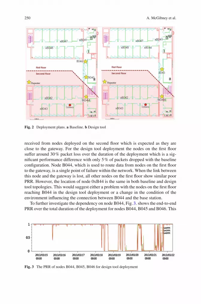
250 A. McGibney et al.

Fig. 2 Deployment plans. a Baseline. b Design tool

received from nodes deployed on the second floor which is expected as they areclose to the gateway. For the design tool deployment the nodes on the first floorsuffer around 30 % packet loss over the duration of the deployment which is a sig-nificant performance difference with only 5 % of packets dropped with the baselineconfiguration. Node B044, which is used to route data from nodes on the first floorto the gateway, is a single point of failure within the network. When the link betweenthis node and the gateway is lost, all other nodes on the first floor show similar poorPRR. However, the location of node 0xB44 is the same in both baseline and designtool topologies. This would suggest either a problem with the nodes on the first floorreaching B044 in the design tool deployment or a change in the condition of theenvironment influencing the connection between B044 and the base station.

To further investigate the dependency on node B044, Fig. 3. shows the end-to-endPRR over the total duration of the deployment for nodes B044, B045 and B046. This

Fig. 3 The PRR of nodes B044, B045, B046 for design tool deployment

Wireless Sensor Networks for Building Monitoring 251

figure shows that the reception of the nodes during the first four days was almostperfect. It may be important to note that the 16th of March is a Saturday and the 17this a Sunday. Suddenly, in the morning of Monday 18th of March, the link begins tofail; the packet reception rate drops to 0 % during the subsequent three nights andremains unstable during the rest of the days until the night of Friday the 22nd. Thesudden poor link quality over, could be attributed to changes in the environmentconditions e.g. the presence of people that may not have been occupied to the sameextent over the weekend period. However the link starts to completely fail duringthe nighttime for long periods of time, and it then continues to have more sporadicconnection loss during the day. As can be seen from the figure the same pattern isobserved for the nodes connected to B044 verifying that the loss of packets from thenodes on the first floor is caused by the failure of the link from the node B044 to thegateway.

The PRR for the baseline deployment resulted in a similar pattern albeit not assevere as the design tool deployment. The overall reception rate is much higher thanthe design tool deployment but this is due to the good quality of the links duringall nights. The majority of the total packet loss ratio (5 %) falls during daytime. Inboth deployments the link between B044 is the most problematic. The exact causeof this is difficulty to establish but it is suggested that a change in the environmentconfiguration (e.g. fire door closed at night) during Design Tool deployment, whichwas not considered by both designs, may have been responsible for the link failures.As devices remained in place for 3 more days (during Easter weekend), additionaldata is also available for the baseline deployment. This shows a very similar pattern tothat of the design tool deployment. All nodes from B044 only managed approximately62 % reliability. Once again, this stresses the possibility of environmental factorsinfluencing the performance of the link between B044 and the gateway and notnecessarily a result of the differences between the design outputs. Received SignalStrength Indicator (RSSI) readings from nodes were used to analyze deeper the causeof failure. Based on previous experiments and as shown in [6], it can be determinedthat when the RSSI values falls below−90 dBm the link quality drastically decreases,and the packet reception rates will in turn decrease. Some links are close to the−90 dBm but on average the most used links remain above this threshold, howeverthese links will be more sensitive to changes in the environment such as interferencesources.

The most problematic link, the one from B044 to the gateway presents an averageRSSI of −79 dBm for both designs. Theoretically, this would not indicate that thelink failure was caused by a weak signal and also that, if minor changes occurwithin the environment, it should be able to absorb the signal degradation. Whenthe RSSI values are analysed for the link between B044 and the gateway over thecomplete deployment period they appear reasonable. As the RSSI is only extractedfrom received data packets, the RSSI is unknown when there is no connection.However, there is no indication from the RSSI that a failure is about to occur. Itis difficult to ascertain exactly the cause of the failure but it has beenshown that the

252 A. McGibney et al.

link between B044 and the gateway is problematic, and also that the design tooldeployment is most affected by this link failure. It is proposed this is due to changesin the environment but it is very difficult to verify this assumption.

6 Lessons Learned

The savings gained by the use of the design tool emphasize the need for support toolsparticularly for indoor environments. However the dynamics of the environment arevery difficult to predict and can result in poor performance no matter how carefulthe design process has been, therefore the tools need to extend beyond design andmore towards holistic management tools. The following are considerations that willbe taken into account as future work [7].

• Link models only provide a “one-shot” prediction and cannot model the complexnature of the environment dynamics

• Tools should bridge the gap between operation and design to learn how to createbetter designs but also to actively adapt a configuration to handle different operatingconditions

• A metric to indicate the dependency of nodes on each other should be provided tothe installer from the design tool output

• The design tool should consider redundancy in its optimization process.

Acknowledgments The authors wish to acknowledge the support of the EU Commission underthe FP7 SCUBA project (Grant Agreement No 288079) in part funding the work reported in thischapter.

References

1. Reinisch, C., Kastner, W., Neugschwandtner, G., Granzer, W.: Wireless technologies in homeand building automation. In: 5th IEEE International Conference on Industrial In-formatics,vol. 1, pp. 93–98 (2007)

2. Itard, L., Meijer, F., Vrins, E., Hoiting, H.: Building Renovation and Modernisation in Eu-rope:State of the Art, review. Jan 2008.

3. Ringwald, M., Romer, K.: Deployment of sensor networks: Problems and passive inspec-tion.In: 5th Workshop on Intelligent Solutions in Embedded Systems (2007)

4. EnOcean Wireless Systems—Range Planning Guide http://www.enocean.com/fileadmin/redaktion/pdf/white_paper/WP_RANGE_PLANNING_Jun09_en.pdf

5. Mc Gibney, A., Guinard, A., Pesch, D.: Wi-design a modelling and optimization tool for wirelessembedded systems in buildings. In: IEEE 36th Conference on Local Computer Networks (LCN)(2011)

6. Srinivasan, K., Levis, P.: RSSI is under appreciated, In: Third Workshop on Embedded Net-worked Sensors (2006)

7. FP7 SCUBA Project http://www.ict-scuba.eu

Long Term WSN Monitoring for EnergyEfficiency in EU Cultural HeritageBuildings

Femi Aderohunmu, Domenico Balsamo, Giacomo Paciand Davide Brunelli

Abstract Historic buildings are a distinctive and invaluable characteristic ofnumerous European cities, and living symbols of Europe’s rich cultural heritage.However, today, EU cultural heritage buildings are contributing huge percentage tothe greenhouse gas emissions. This has led to the increasing of wireless sensor net-work (WSN) deployments aimed at monitoring and improving the energy efficiencyof these historic buildings. In this chapter we show a long term, low cost, passive dis-tributed environmental monitoring system that promotes energy-efficient retrofittingin historic buildings. We focus on the design and implementation of an innovativetechnological framework, and on the hardware and software development of the solu-tion. The presented system provides real-time feedback for the civil engineers forprompt intervention via remote interfaces.

1 Introduction

Intelligent monitoring of the structural health of historic buildings has become animportant research problem domain. Particularly, due to the lack of pre-existing mon-

F. AderohunmuInformation Science Department, University of Otago, Dunedin, New Zealande-mail: femi.aderohunmu@otago.ac.nz

D. Balsamo · G. PaciDepartment of Electrical, Electronic and Information Engineering (DEI),University of Bologna, Bologna, Italye-mail: domenico.balsamo@unibo.it

G. Pacie-mail: giacomo.paci@unibo.it

D. Brunelli (B)

Department of Industrial Engineering (DII), University of Trento,Via Sommarive 14, Trento, Italye-mail: davide.brunelli@unitn.it

K. Langendoen et al. (eds.), Real-World Wireless Sensor Networks, 253Lecture Notes in Electrical Engineering 281, DOI: 10.1007/978-3-319-03071-5_25,© Springer International Publishing Switzerland 2014

254 F. Aderohunmu et al.

Fig. 1 a Heritage building with WSN deployment. b Hardware unit: A rear view of 32-bit WISPESW24th prototype

itoring models and to the constraints associated with the measurement devices. Withthe increasing ease of fast prototyping and low cost of manufacturing, miniaturizedsmart sensor nodes can be easily configured for monitoring purposes, today. Thechallenge is however, the ability to allow these nodes to operate in a collaborativemanner over a long period of time without user intervention. The development ofsuch architectures require a cross layer design from hardware and network perspec-tive to the application layer. In this chapter we introduce an application scenario andwe present a design testbed and the implementation strategies for a rapid, accurateand low-cost intelligent monitoring. The selected hardware allows low power con-sumption and long distance peer-to-peer data transmission. The software design isan open source built on the NXP Jennic platform [12]. It supports star, tree and linearnetwork topologies. An integrated prototype has been deployed in a 36-nodes WSNtestbed in a 4-storey renaissance building of about 1300 m2, see Fig. 1a. The buildingis currently hosting several employees and students, and at the same time containsimportant historical artworks and frescoes. One of the main source of concerns forthe local conservation board is how to preserve these artworks. It is necessary to con-duct a timely estimation of any potential risk that could damage the building. Thisrequires a real-time monitoring and an appropriate response model that can alloweasy reproduction of the structural characteristics of the building.

The goal of the work is to develop a low-power, long-term and low-cost hard-ware and software solution that can efficiently monitor local climate changes inthe building. Our design consists of WISPES 24th node type [20], which gathersenvironmental parameters such as, air temperature, relative humidity, vibration, gasconcentration, air quality and ambient light. The network delivers data through amulti-hop network topology.

The remainder of this chapter is organized as follows: In Sect. 2 we present theapplication scenario, followed by the description of the hardware prototype in Sect. 3.In Sect. 4 we describe a proprietary software stack architecture that has been adaptedspecifically to meet the needs for low-cost, long-term and low-power operationallife-cycle. In Sect. 5 we present our deployment testbed, it is worth mentioning that,the deployment has currently spanned 18 months and it is assessed to be in the halfof the lifetime. Finally, in Sect. 6 we conclude the chapter.

Long Term WSN Monitoring for Energy Efficiency 255

2 Application Scenario

Structural health monitoring of building is a critical component of the civilinfrastructure system. For instance, heritage buildings are often on the lookoutfor health monitoring by civil engineers due to their touristic attraction towardsthe public. The safety of such buildings is necessary to limit the danger it posesto the economic vitality of the society especially during damaging events such asearthquake etc. The conservation of such structures for the future generations is oneof the main tasks of the European Union (EU). It is increasingly becoming impor-tant to understand the deterioration processes which affect artworks in museums andhistoric buildings, [9, 21]. Preserving the health of such structures requires a con-tinuous monitoring process of the building [2]. Some of the parameters of interestare temperature, humidity, dust presence, quality of the air, etc. Apart from monitor-ing the health of the building structures, some of the heritage buildings contain somehistorical artifacts and frescoes that require a certain temperature and humidity levelsfor easy preservation.

The development in the fields of micro-electromechanical systems and wirelesscommunications have introduced easy and low cost monitoring of such buildings,[1] and [13]. Therefore, it is possible to develop low-power, easy to install andminiaturized gadgets to sense and transmit data at a reasonable distance to morepowerful gateway nodes equipped with high computational capabilities in place of thecommon commercial cabling system that is often utilized. Similar application designusing WSN have been used in recent years. In Villa Regina [15], authors deployeda monitoring system composed of a wireless network of smart buttons, specificallydesigned to satisfy the requirements for applications in the field of cultural heritage.Majority of their work focused on evaluating the reliability of WSN for protecting andpreventing the oxidation of old mirrors. Similarly, in the case study of Torre Aquila[7]; a medieval tower in Trento (Italy), where a customized hardware efficientlycollects high-volume vibration data using specially designed sensors to acquire thebuilding’s deformation. One of the main drawbacks of these existing deployments isthat, the majority of the implementations do not support ultralow power operation,thus hampering their use for a long-term deployment. Since the lifetime of a WSNdepends largely on the power consumption at each sensor node, we focused onreducing power consumption both when the node is in active mode and when thenode is in sleep mode. We are able to achieve this by optimizing the radio activitythrough a synchronous power management strategy and through a dynamic powercontrol algorithm. This minimizes the use of the DC–DC converter, which guaranteesa stable input voltage reference when the system is in ‘ON’ mode. In the next section,we describe the hardware unit for our monitoring application.

256 F. Aderohunmu et al.

Table 1 Summary of theenergy consumption for onecycle of the state machine

Sample rate No transmission (mJ) Transmission (mJ)

10 s 8.184 27.8941 min 9.5 29.2110 min 23.72 43.43

3 Sensing Unit and Hardware Design

The hardware unit is shown in Fig. 1b. The sensor node is built on the NXP JN5148module with interconnected on-board sensors. The core of this module is designed tomeet the requirements of ZigBee PRO applications, nevertheless we optimized thenetwork protocol with proprietary features. The W24th nodes are equipped with thefollowing on-board sensors: Temperature (0.01 ◦C resolution; −40 to +90 ◦C. range),Humidity (0.04 ◦C resolution; 0–100 % rh range), Light sensor (0.23 lx resolution;0–100,000 lx range), 3-axis accelerometer (1 mg resolution; 0–6 g) and MOX Gassensor interface (10 % resolution). Our prototype incorporates an integrated hardwareand software designs that is capable of supporting both tree and star topologies.The flexibility of the hardware permits the W24th node to serve indifferently asa coordinator node, sleep-end node or router depending on the chosen topology.Through the wireless communication channel, the coordinator node can broadcastpackets to the entire network, and the network can be organized. The sensing unitsare able to sense all the previously mentioned parameters, store the data, analyze andtransmit the data when necessary Table 1.

The core of the system is a 32 bit micro-controller with a 2.4 GHz radio transceiverthat can achieve about 100 m communication range in an indoor-environment. The32 Mhz CPU clock permits the development of distributed data processing applica-tions with the possibility of attaching an external memory slot i.e., W24th is equippedwith a microSD card reader for local storage, data logging and backups. This allowsthe W24th to be connected to several expansion boards such as multi-channels acqui-sition interfaces, actuators, USB, KNX devices, energy harvesters and more [6, 10,18, 19]. Often in the field of wireless sensor networks, wireless communication isknown to be one of the major sources of power consumption. Long range commu-nication is normally avoided as it increases the power drainage of the transceiver. Inambient monitoring application, communication range could be up to hundreds ofmeters. It is imperative to avoid constant transmission when not necessary to prolongthe battery life. It is possible to achieve local data processing such as aggregationfrom cluster-heads or coordinator node due to the support of a peer-to-peer communi-cation offered by nodes. The W24th uses an aggressive power management methodusing 8µA in sleep mode, 17 mA in transmit mode and 23 mA in receive mode,which guarantees a longer battery lifetime. For example, compared with a TelosBmote [8], our node platform is able to yield about 35 % more power savings. Theraw data transfer rate of the transceiver is up to 26 kps when used on the communi-cation protocol and it includes reliable re-transmission/acknowledgment procedureaccording to the IEEE 802.15.4 standard.

Long Term WSN Monitoring for Energy Efficiency 257

Dynamic power-supply control In our test deployment one of the focus is toreduce the overall power consumption both when the node is in active mode andin the sleep mode. In the active mode, we achieved a reduced power consumptionby optimizing the radio activity through a synchronous power management strategy.Similarly, in the sleep mode, reduced power consumption is achieved by imple-menting a dynamic power-supply control algorithm, which minimizes the use of theDC–DC converter.

We implement a novel technique for extending the lifetime of a WSN node, byminimizing the consumption of the DC–DC converter during sleep mode. This isaccomplished through an adaptive algorithm that turns ‘ON’ and ‘OFF’ a DC–DCconverter to minimize the on-board sleep power consumption. DC–DC converters,typically, need an output capacitor for high frequency ripple filtering. The adaptivealgorithm computes on-line the maximum interval which guarantees the node tooperate solely with output capacitor, taking into account both the total leakage and itsvariations under temperature changes. The proposed solution significantly increasesthe lifetime of applications with low-duty cycle activity, such as WSNs, achieving inthe performed test a lifetime increment of over 30 %. In this way, the system allowsa reliably data transfer and so far has an estimated lifetime beyond three years in fulldeployment.

4 Software and Protocol Stack Architecture

The protocol stack design for our intelligent monitoring application is built on theJennic platform [12] developed on the IEEE 802.15.4 standard, which operates inthe globally unlicensed 2.4 GHz band. Our network design consists of a Coordinatornode which serves as the sink node (central server), some Router nodes and severalSleep-End nodes.

The Jennic platform ensures real-time data logging at the Coordinator node due tothe memory management strategy in place. The design of the protocol stack has thefollowing features: (1) Network load balancing to avoid data throughput congestion;(2) Offers support to the Sleeping End nodes for extended battery life; (3) Providesend-to-end message acknowledgment; (4) Allows over-the-air download; (5) Pro-vides statistics for network maintenance (6) Supports automatic route formation andrepair in-case of routing and (7) Finally, it provides network re-shaping to reducenetwork depth. In addition to these features, one of the main characteristic of theJennic platform is that it can efficiently handle all the network traffic and can man-age network faults with a self-healing mechanism. All these features make Jennicplatform a choice for our WISPES W24th node prototype.

258 F. Aderohunmu et al.

4.1 Time Synchronization

Time synchronization is a fundamental service in many distributed systems. Non-uniform operating temperature among deployed nodes and dynamic variation of thetemperature is the major cause of clock drift in the nodes of a network. In this networkprotocol we implemented a low-overhead clock synchronization for WSNs based ona new temperature compensation algorithm (TCA) presented in [3]. The TCA is localand uses a temperature sensor to remove the effects of environmental temperaturechanges and to increase the time between synchronization intervals. Using the TCA,the 32 KHz unit achieves an effective clock drift of less than 5 ppm over a wide rangeof operating temperatures (−5 to 62 ◦C), a significant improvement with respect tothe 55 ppm featured without temperature compensation.

This allows the coordinator node to broadcast beacons signals for all nodes inthe network to synchronize their time-stamp, and then all the node including routercan switch to the sleep mode, shutting down the radio. In the compensated node,the maximum drift is about 100 us, every 20 s, across the full temperature range;this means that a deviation in the network of 1 s may happen only after 55 h in anypossible temperature condition. This synchronization accuracy is enough to put allthe nodes of the networks (including routers) in sleep mode.

Moreover, the goal of our platform design is to be able to support other topologies,thus our design strategy deviates from the beacon-enabled approach. We instead use anon-beacon-based approach, which does not provide time synchronization and it doesnot support the active/sleep scheduling and Guarantee Time Slot (GTS) mechanism.It however, exhibits certain features, such as high scalability and low complexitythat makes it a method of choice for our design. To be able to use the non-beacon-based approach, we need to re-design a method to synchronize the network. As aresult, exploiting the temperature compensation algorithm (TCA), we implementedalso an Energy-efficient Service-Packet-based (ESS) transmission scheduling algo-rithm. This method is based on a centralize approach that is capable of providingtime synchronization on the top of the non-beacon-enabled IEEE 802.15.4 standard.The algorithm is designed to avoid collision in the network during packet trans-mission through a TDMA technique. The service-packet contains the time stampand other necessary network information such as the active sensors on the network.The service-packet transmission across the network is achieved by using a novelmethod based on constructive interference of IEEE 802.15.4 symbols for fast net-work flooding and implicit time synchronization. The overall idea is that interferenceis considered an advantage rather than a problem. Based on this intuition, the simul-taneous transmission of packet in the network becomes constructive. This methodhas proven to achieve a flooding reliability above 99 %, [11] which is quite close tothe theoretical lower latency bound. Our method proves to achieve a network-widetime synchronization at no cost since it implicitly synchronizes the nodes as theflooding packets propagates through the network. With this approach, the nodes turnon their radios, listen for communications over the wireless medium, and transmitover-heard packets after a certain time delay. Moreover, since the neighbours of a

Long Term WSN Monitoring for Energy Efficiency 259

Fig. 2 Deployment map (a) comparison between illuminance measurements taken using bothlux-meter and the deployed WSN (b)

sender recieves packet at the same time, they also transmit the packets at the sametime.

One key strategy to ensure that a received packet has been relayed, is to allow eachnode decrement an internal counter for the number of Service Packet transmitted.To summarize, the network node achieves synchronization by using service packetsand the coordinator defines the network topology for the deployment based on theavailable Link Quality and finally, it schedules each node to their given time-slot.

5 Deployment

Our deployment consists of 36-node setup located in the different parts of a 4-storeyhistoric building shown in Fig. 2a. The reason for the different positions of the nodesis to be able to capture various characteristics of environmental variables across thebuilding. For example, the first-floor contains ventilation systems that are constantlyinterrupted by the occupants; the attic contains generators and it is more closer tothe roof (outside) temperature, while the underground floor has less interaction.Understanding the dynamics of the occupancy with respect to the characteristics ofthe building is of interest to the civil engineers we interacted with. In our deployment,13 nodes are used as mobile stations for specific measurement purpose. These nodescan be used for dynamic surveys and may be employed to confirm the data collectedby alternative testing techniques.

The huge amount of data generated by different sensors is handled using Compres-sive Sensing algorithms [4, 5]. We present here only the illuminance measurementinside one of the rooms by using both professional lux-meter and 13 WSN nodes(Fig. 2b). Notice that this comparison demonstrates how our nodes, equipped with

260 F. Aderohunmu et al.

light sensors, can be used in place of the professional lux-meter to achieve a contin-uously monitoring of the daily or seasonal variations of ambient light with minimalefforts and errors on the measurements.

6 Conclusion

In this chapter, we describe the design and the implementation of a Wireless SensorNetwork tailored for monitoring heritage buildings. The continuous monitoring ofenvironmental parameters is crucial for protecting cultural heritage and historicalbuildings. In this type of application, wireless sensor networks represent an alterna-tive to traditional measuring instrumentations. The use of WSNs guarantees low-costand long-term monitoring with a high rate of data extracted from the deploymentfor further analysis. The network will be enhanced with Smart Wireless PowerMeters [16, 17] and Multimodal Video Sensor Nodes [14] as future works. The pro-posed sensor network includes functionalities for network management and efficientpower supply management and provides real-time feedback for the civil engineers.

Acknowledgments The research leading to these results has received funding from the projects3ENCULT and GreenDataNet, both funded by the EU 7th Framework Programme. In addition, theauthors would like to thank WISPES srl for the implementation of the prototypes

References

1. Abrardo, A., Balucanti, L., Belleschi, M., Carretti, C., Mecocci, A.: Health monitoring ofarchitectural heritage: the case study of san gimignano. In: Environmental Energy and StructuralMonitoring Systems (EESMS), 2010 IEEE Workshop on, pp. 98–102, 2010

2. Anastasi, G., Lo Re, G., Ortolani, M.: wsns for structural health monitoring of historicalbuildings. In: Human System Interactions, 2009. HSI ’09. 2nd Conference on, pp. 574–579,2009

3. Brunelli, D., Balsamo, D., Paci, G., Benini, L.: Temperature compensated time synchronisationin wireless sensor networks. Electron. Lett. 48(16), 1026–1028 (2012)

4. Caione, C., Brunelli, D., Benini, L.: Distributed compressive sampling for lifetime optimizationin dense wireless sensor networks. IEEE Trans. Industr. Inf. 8(1), 30–40 (2012)

5. Caione, C., Brunelli, D., Benini, L.: Compressive sensing optimization for signal ensemblesin wsns. Industrial Informatics, IEEE Transactions on (2013)

6. Carli, D., Brunelli, D., Benini, L., Ruggeri, M.: An effective multi-source energy harvesterfor low power applications. In: Design, Automation Test in Europe Conference Exhibition(DATE), pp. 1–6, 2011

7. Ceriotti, M., Mottola, L., Picco, G. P., Murphy, A. L., Guna, S., Corra, M., Pozzi, M., Zonta,D., Zanon, P.: Monitoring heritage buildings with wireless sensor networks: the torre aquiladeployment. In: Proceedings of the 2009 International Conference on Information Processingin Sensor Networks, IPSN ’09, pp. 277–288, Washington, DC, USA, 2009. IEEE ComputerSociety.

8. Crossbow. http://www.xbow.com (1995). Accessed 8 Sept 2012

Long Term WSN Monitoring for Energy Efficiency 261

9. Amato, F. D’., Gamba, P., Goldoni, E.: Monitoring heritage buildings and artworks with wirelesssensor networks. In: Environmental Energy and Structural Monitoring Systems (EESMS), 2012IEEE Workshop on, pp. 1–6, 2012

10. Dondi, D., Bertacchini, A., Larcher, L., Pavan, P., Brunelli, D., Benini, L.: A solar energyharvesting circuit for low power applications. In: Sustainable Energy Technologies, 2008.ICSET 2008. IEEE International Conference on, pp. 945–949, 2008

11. Ferrari, F., Zimmerling, M., Thiele, L., Saukh, O.: Efficient network flooding and time syn-chronization with glossy. In: IPSN, pp. 73–84, 2011

12. Jennic-Platform. NXP Jennic platform. http://www.jennic.com/index.php (1996)13. Lynch, J. P.: Overview of wireless sensors for real-time health monitoring of civil structures.

In: The 4th Intern. Workshop on Structural, Control, 10–11 June 200414. Magno, M., Brunelli, D., Zappi, P., Benini, L.: A solar-powered video sensor node for energy

efficient multimodal surveillance. In: Digital System Design Architectures, Methods and Tools,2008. DSD ’08. 11th EUROMICRO Conference on, pp. 512–519, 2008

15. Neri, A.,et al.: Environmental monitoring of heritage buildings. In: Environmental, Energy,and Structural Monitoring Systems, 2009. EESMS 2009. IEEE Workshop on, pp. 93–97, 2009

16. Porcarelli, D., Balsamo, D., Brunelli, D., Paci, G.: Perpetual and low-cost power meter for mon-itoring residential and industrial appliances. In: Design, Automation Test in Europe ConferenceExhibition (DATE), pp. 1155–1160, 2013

17. Porcarelli, D., Brunelli, D., Benini, L.: Clamp-and-measure forever: A mosfet-based circuit forenergy harvesting and measurement targeted for power meters. In: Advances in Sensors andInterfaces (IWASI), 2013 5th IEEE International Workshop on, pp.200–205, 2013

18. Porcarelli, D., Brunelli, D., Magno, M., Benini, L.: A multi-harvester architecture with hybridstorage devices and smart capabilities for low power systems. In: Power Electronics, ElectricalDrives, Automation and Motion (SPEEDAM), 2012 International Symposium on, pp. 946–951,2012

19. Weddell, A.S., Magno, M., Merrett, G.V., Brunelli, D., Al-Hashimi, B.M., Benini, L.: A surveyof multi-source energy harvesting systems. In: Design, Automation Test in Europe ConferenceExhibition (DATE), pp. 905–908, 2013

20. WISPES. Wispes W24TH sensor node. http://www.wispes.com (2009)21. Zonta, D., Pozzi, M., Zanon, P.: Managing the historical heritage using distributed technologies.

Int. J. Architectural Heritage 2(3), 200–225 (2008)