Recent behavior of output, unemployment, wages and prices

in Colombia: What went wrong?

Luis E. Arango, Ana M. Iregui and Luis F. Melo*

Banco de la República

May 2003

Abstract At the end of the last decade, the real activity in Colombia underwent the sharpest recession of the last fifty years. We postulate a non-triangular structural VAR model (Amisano and Giannini, 1997) to describe the dynamics of output, prices, unemployment and wages during the last two decades. The evidence suggests that, in the long-run, monetary policy has been neutral to both output and unemployment while the main reasons for the increase in the latter have been the lack of credibility of monetary policy, the way in which wages are set and the increase in non-wage labor costs.

Key words: structural VAR, unemployment, monetary policy, wages, expectations. JEL classification: E24, C40.

* The opinions expressed here are those of the authors and do not necessarily represent neither those of the Banco de la República nor of its Board of Directors. The authors thank Franz Hamman, Marta Misas, Jesús Otero, Carlos Esteban Posada, Hernando Vargas, and Diego Vásquez for helpful comments and suggestions and Mario Ramos for valuable research assistance. The usual disclaimers apply.

1

1. Introduction At the end of the 1990s the Colombian economic activity suffered the sharpest recession of the

last fifty years to the extent that output decreased about 5% in 1999. In addition, the

unemployment rate started to rise consistently reaching 20% in the year 2000. This increase in

the unemployment rate was accompanied by a gradual reduction in inflation and an increase in

real wages.

In view of these facts, to explain the slowdown of the economic activity several reasons

have been put forward. Among the arguments are: i) the tighter monetary policy set by an

authority committed with an inflation reduction program; ii) the lack of credibility of monetary

policy; iii) the type of expectations formed by agents when setting nominal wages which put

wages above their long-run equilibrium level (Arango and Posada, 2001, 2002). Urrutia (2002)

provides another explanation of the recession of 1999 which is linked to the deficit of the

current account and the sudden stop of capital flows associated to the crises of the international

capital markets occurred in 1997. However, we do not emphasize this view in our work. Instead,

we highlight the other three explanations since we understand that the most important causes of

the recession were internal rather than external.

Accordingly, we postulate a structural VAR model for a closed economy to describe the

dynamics of output, unemployment, wages and prices during the last two decades. Such an

approach has been previously used to study some macroeconomic aspects in different

economies. For example, Dolado and Jimeno (1997) associate the causes of Spanish

unemployment with shocks of different nature which have long lasting effects due to a full

hysteresis phenomenon. They find that the “… dismal performance of Spanish unemployment

can be explained as the result of a series of adverse shocks, which were difficult to absorb in a

context of a rigid system of labor market institutions and disinflationary policies. This finding

has relevant policy implications that unless supply side reforms are implemented, deflationary

policies will continue to be very costly in unemployment terms”(p. 1285).

Balmaseda et al. (2000)1 focus on the role played by aggregate demand, productivity,

and labor supply shocks in explaining the joint dynamic behavior of real output, real wages and

the unemployment rate in the modeling of labor markets in a sample of 16 OECD economies

over the period 1950-96. They find that “in most countries the identification scheme based on

2

unemployment being persistent but stationary yields more reasonable results than those based on

full-hysteresis whereby unemployment is considered to be an I(1) variable” (p.22). In addition,

the authors find that unemployment fluctuations are dominated by aggregate demand shocks in

the short-run and by labor supply and productivity shocks at lower frequencies.

For the case of Colombia, Misas and López (1998, 2001) use a SVAR (Blanchard and

Quah, 1989) approach to estimate output and unemployment gaps, whereas Misas and Posada

(2000) examine the sources of variation of the unexpected component of output growth. Arango

(1998) obtains some evidence on the nature (either nominal or real) of the temporary and

permanent components of the Colombian output and prices. Finally, Restrepo (1997) uses a

VAR approach to explain the response of some macroeconomic variables (GDP, real exchange

rate index, real money balances, money, inflation, and interest rate) to supply, demand, money

demand and money supply shocks.

However, our work advances some of them since we present and solve a stylized model

for the Colombian economy and introduce, in the empirical model, the long run restrictions

provided by the theoretical framework2. The evidence provided by this work suggests that, in

the long-run, monetary policy has been neutral to both output and unemployment while the main

reasons for the increase in the latter have been the lack of credibility of monetary policy, the

way in which wages are set (both of which increased the real wage) and the increase in labor

costs other than wages, such as those introduced by pension reforms3.

The outline of the paper is as follows. Section 2 presents some facts related to the

macroeconomic performance of the Colombian economy during the last years. Section 3

introduces the model. Section 4 presents the methodology and the empirical application. Section

5 presents a discussion of our findings and section 6 provides some concluding remarks.

2. The facts Since 1991 the Colombian central bank has been conducting a program for reducing inflation.

Such a program has been characterized by targets that decrease gradually, accompanied, among

1 See also Algan (2001) and Fabiani et al. (2001). 2 Arango (1998) also presents and solves a small macro model. 3 By using a different approach Cárdenas and Gutiérrez (1998) also underline the increase in nonwage labor costs as one of the determinants of the rise in the unemployment rate. However, other aspects such as the appreciation of the Colombian peso and the increase in the value added tax have also played a role in their view.

3

other things, by consistent stances of monetary policy4. On the one hand, the policy was

effective in the sense that, since then, inflation showed a negative-sloped long run component

(see Figure 1).

Figure 1. Annual inflation rate

7%

12%

17%

22%

27%

32%

1984

1985

1986

1987

1988

1989

1990

1991

1992

1993

1994

1995

1996

1997

1998

1999

2000

Observed inflation rate Annual inflation targets

Source: DANE and Banco de la República-SGEE

On the other hand, the program for reducing inflation was somehow intricate in the sense

that no inflation target was reached until 1997 (see Figure 1), a fact that, without any doubt,

undermined the credibility of the monetary authority5. In 1998 the authorities missed the target

again; in 1999 and 2000 the observed inflation levels were of 9.2% and 8.8% while the targets were

15% and 10%, respectively. These results might have suggested of a monetary policy stance tighter

than required6.

To complete the picture, in the late 1990s Colombia experienced a sharp recession as panels

A, B, and C of Figure 2 show. The growth of real output and the employment rate underwent an

abrupt reduction (Panel A) while the unemployment rate of the seven major cities of the

country7 soared between 1994 and 1999 (Panel B). We use two measures of the unemployment

rate: the first one is defined as “one minus the occupation rate”, which rose from 44% to about

50% between 1994 and 2000, whereas the second measure, defined as “one minus the ratio of

the occupation rate to the participation rate”, increased to about 20% during the same period. 4 See Urrutia (2002) for an interpretation of the monetary policy during the last decade. See also Hernández and Tolosa (2001). 5 In 1997 the inflation target was 18% while the observed inflation was 17,7%. 6 By that time, an intricate international environment for emerging markets together with internal fiscal difficulties and a current account imbalance were also part of the picture (see Urrutia, 2002). However, our analysis shall not focus explicitly on these aspects.

4

We make this distinction since the first measure of unemployment is the one that results from

our model and so we use it in the empirical exercise, while the second measure is the one

officially published. Finally, Panel C shows the urban employment rate which exhibits a strong

reduction during the same period. However, against some beliefs, the period of inflation

reduction and increase in the unemployment rate (our second measure) are far from coincident

(Figure 3). This is because inflation started to fall in 1991 while unemployment started to rise in

1994.

Figure 2. Evidence of the slump in Colombia in late 1990´s

A. Annual growth rate of output and employment rate

-10%

-6%

-2%

2%

6%

10%

1985

1986

1987

1988

1989

1990

1991

1992

1993

1994

1995

1996

1997

1998

1999

2000

-8%

-4%

0%

4%

8%

Annual quarterly GDP growth Employment growth rate

B. Unemployment rates (seven cities)

42%

45%

48%

51%

54%

1984

1985

1986

1987

1988

1989

1990

1991

1992

1993

1994

1995

1996

1997

1998

1999

2000

7%

10%

13%

16%

19%

22%

(1 - employment rate) Unemployment rate

C. Employment (occupation) rate (seven cities)

0,46

0,48

0,50

0,52

0,54

0,56

1984

1985

1986

1987

1988

1989

1990

1991

1992

1993

1994

1995

1996

1997

1998

1999

2000

Source: DANE-DNP, Banco de la República-SGEE and authors´ calculations

Figure 4 shows the unemployment rate (as measured by “one minus the occupation

rate”) and (the log of) the real labor income index, based on labor income data taken from the

Encuesta Nacional de Hogares (National Housing Survey) deflated by the CPI, which is the

7 These cities account for about 75% of the total population of the country.

5

proxy we use for the real wage index. According to the figure, this period was characterized,

firstly, by a sharp increase in the unemployment rate: 1994 – 1999, and, secondly, by an

inconsistent strong wage growth that started in mid 1992.

Figure 3. Inflation and unemployment rate

7%

11%

15%

19%

23%

27%

31%

35%

1984

1985

1986

1987

1988

1989

1990

1991

1992

1993

1994

1995

1996

1997

1998

1999

2000

7%

10%

13%

16%

19%

22%

Observed inflation rate Unemployment rate

Source: DANE-DNP, Banco de la República-SGEE and authors´ calculations

The hypothesis we maintain is that the increase in the unemployment rate was a reaction

to a real wage growth out of the equilibrium path (Arango and Posada, 2002) that converted

labor in a very costly factor8. The behavior of the real wage might be the result, on the one hand,

of an unexpected reduction in the inflation rate, perhaps due to the combination of a backward-

formed expectations phenomenon and low credibility of the monetary policy. On the other hand,

the behavior of the real wage might be the result of a minimum wage policy that sometimes

leads other nominal wage settings in the country, whose level is established on political rather

than factual (economic) grounds.

Just before the unemployment rate started to rise in 1994, the Law 100 of 1993, a new

labor market and social security legislation was enacted. Under this new scheme, some of the

labor costs related to health and pension plans were augmented (see Arango and Posada, 2001).

Figure 5 shows the behavior of the labor costs, other than real wages, and the unemployment

rate. Accordingly, the above hypothesis -related to the expectations and effects of the minimum

wage policy- could be amended to consider the impact of the increase in labor costs introduced

8 Iregui and Otero (2002), through nonlinear techniques, make the point that wages above their long-run equilibrium level do increase unemployment, but wages below this level do not reduce it. This result supports the view that factors that increase unemployment are not the same as those reducing it.

6

by such legislation. As a result, labor became rather costly at the beginning of the second half of

the nineties. Figure 4. Unemployment rate and real wage index

42%

45%

48%

51%

54%

1984

1985

1986

1987

1988

1989

1990

1991

1992

1993

1994

1995

1996

1997

1998

1999

2000

85

95

105

115

125

135

(1- employment rate) Real wage index Source: DANE-DNP, authors´ calculations

Figure 5. Unemployment rate and labor costs other than wages

42%

45%

48%

51%

54%

1984

1985

1986

1987

1988

1989

1990

1991

1992

1993

1994

1995

1996

1997

1998

1999

2000

Non-wage labor costs (1- employment rate)

Source: DANE, Arango and Posada (2001).

3. A stylized model To rationalize the above facts we use a model consisting of a set of structural equations (all

variables are in logs):

ttdt pmy −= (1)

ttttst pEpy θγ +−= − )( 1 (2)

ttttdt cypwn ϕβα −+−−= )( (3)

tttst pwn τδ +−= )( (4)

7

where dty stands for aggregate demand in period t, s

ty for aggregate supply, tp for the price

level, tθ for the technology process, dtn for labor demand, s

tn for labor supply, tw for

nominal wage, tc for the labor costs different from the wage, and tτ for a labor-supply shift

factor (Balmaseda et al, 2000). tE is the expectations operator.

Equation (1) suggests that aggregate demand responds to real balances as in the quantity

theory setting. Equation (2) assumes that aggregate supply is moved by two factors: technology

and surprises in the price level or, in other words, deviations of observed prices from expected

prices (Sargent and Wallace, 1975). Equation (3) sets that labor demand depends on real wages,

economic activity and labor costs different from real wages. Variable tc reflects costs such as

social security contributions (health and pension plans) and other payroll taxes such as the

contributions to the Instituto Colombiano de Bienestar Familiar (ICBF), the Servicio Nacional

de Aprendizaje (SENA) and the Cajas de Compensación Familiar9 (see Figure 5).

In addition, the model contains the following two definitions: dt

stt nnu −= (5)

ttttt pEw θλτρ +−= −1 (6)

where tu is the unemployment rate.

Finally, it is assumed that tm , tθ , tc and tτ behave as random walks10:

mttt mm ε+= −1 (7)

θεθθ ttt += −1 (8)

τεττ ttt += −1 (9)

cttt cc ε+= −1 (10)

The solution of the model is given by:

9 The ICBF attends issues related to the welfare of family, women, childhood and third age, The SENA is an official agency committed to training of labor force; the Cajas receive contributions for leisure, training and health of the labor force and families of the workers. 10 We also included a drift in equation (8). However, the long run restrictions of the system did not change.

8

θθ εγ

γεγ

εεγ

γ11 11

1)(1 −− +

++

+−+

=∆ ttmt

mtty (11)

ctt

tttmt

mtt AAu

εϕεαρδρ

εβδλαλεεεετ

θθθ

+−−+

−++−+−−=∆ −−

)1(

)()()( 11 (12)

τθθ ερεελε tttmttw −−+=∆ −− 11 (13)

θθ εγ

γεγ

εγ

γεγ 11 11

111

1−− +

−+

−+

++

=∆ ttmt

mttp (14)

where [ ]γδβγα +++= 1A , and ]][)1(1[ θεεγ tmt −+ corresponds to the contemporary

inflationary surprise.

Accordingly, in this economy only technology shocks have permanent effects on y 11.

Technology, labor supply and ex-wage labor costs shocks have permanent effects on u .

Technology, nominal and labor supply shocks have permanent effects on w and both

technology and nominal shocks have permanent effects on p . By looking at the restrictions

that emerge from the model, it is obvious that no triangular matrix is useful for identifying the

shocks. Next we explain the methodology.

4. Empirical approach We use a Blanchard-Quah (1989) style non-triangular decomposition to identify a SVAR model

of output ( y ), unemployment rate ( u ), nominal wages ( w ) and prices ( p ) for the period

1984:1 – 2000:4. Each variable was entered into the model in log levels, with the exception of

the unemployment rate which was entered as a fraction.

The statistical tests indicate that these series are integrated of order one each12 and that

no cointegrating relationship arises among them. Taking into account these stochastic properties

11 The long run restriction of the nominal shock stems from the fact that the polynomial of lags that relates this shock to the first difference of y is zero when it is evaluated with the lag operator equal to one. This type of restriction is used by Blanchard and Quah (1989) among others. 12 The persistence of unemployment rate is related to the so-called hysteresis phenomenon (Blanchard and Summers, 1986). However, the persistence of unemployment rate in Colombia seems to arise because of the behaviour during the second half of 1990´s (Arango and Posada, 2001).

9

we estimate a VAR model of order two for the first difference of the selected series13. The

selected reduced-form VAR model can be expressed as:

TtLA tt ,,2,1,eX)( …==∆ (15)

where ( )tttt pwuy ,,,X't = , p

p LALAILA −−−= …1)( , with L as the lag operator, p=2 and

{ }te a Gaussian white noise process with covariance matrix Σ . The model (15) can also be

noted in terms of structural shocks as:

ttLB ε=∆X)( (16)

where pp LBLBBLB −−−= …10)( and { }tε is a Gaussian white noise process with covariance

matrix I . In our case the structural shocks correspond to =′tε ( )ctt

mtt εεεε τθ ,,, . By using the

Wold theorem, expression (15) can be written in terms of reduced form shocks:

tt LC eX )(=∆ (17)

or in terms of structural shocks as:

tt L ε)(Φ=∆X (18)

where, …+++= 221)( LCLCILC and …+++=Φ 2

210)( LLL φφφ

Based on expressions (17) and (18) it can be shown that structural and reduced form

shocks are related to each other as follows:

tte εφ0= (19)

Since the series included in the model are I(1) processes, the long-run restrictions, in

terms of the structural shocks, can be formulated using the elements of )1(Φ :

∂∂

∂∂

∂∂

∂∂

∂∂

∂∂

∂∂

∂∂

∂∂

∂∂

∂∂∂

∂∂

∂∂

∂∂

∂∂

=

=Φ

−∞→

−∞→

−∞→

−∞→

−∞→

−∞→

−∞→

−∞→

−∞→

−∞→

−∞→

−∞→

−∞→

−∞→

−∞→

−∞→

∞

=

∞

=

∞

=

∞

=

∞

=

∞

=

∞

=

∞

=

∞

=

∞

=

∞

=

∞

=

∞

=

∞

=

∞

=

∞

=

∑∑∑∑

∑∑∑∑

∑∑∑∑

∑∑∑∑

ckt

tk

kt

tkm

kt

tk

kt

tk

ckt

tk

kt

tkm

kt

tk

kt

tk

ckt

tk

kt

tkm

kt

tk

kt

tk

ckt

tk

kt

tkm

kt

tk

kt

tk

ii

ii

ii

ii

ii

ii

ii

ii

ii

ii

ii

ii

ii

ii

ii

ii

pppp

wwww

uuuu

yyyy

εεεε

εεεε

εεεε

εεεε

φφφφ

φφφφ

φφφφ

φφφφ

τθ

τθ

τθ

τθ

limlimlimlim

limlimlimlim

limlimlimlim

limlimlimlim

)1(

044,

043,

042,

041,

034,

033,

032,

031,

024,

023,

022,

021,

014,

013,

012,

011,

13 The number of lags was chosen to be the minimum for which we obtain Gaussian white noise residuals. The diagnostic statistics for the residuals of the model are presented in Appendix 1.

10

Accordingly, with the economic constrains implied by the model of the previous section,

we have the following restrictions:

ΦΦΦΦΦ

ΦΦΦΦ

=Φ

00)1()1(0)1()1()1(

)1()1(0)1(000)1(

)1(

4241

333231

242321

11

(20)

where the first row shows the long run response of y to the shocks θε , mε , τε and cε

respectively; the second, third and fourth row shows the response of u , w , and p ,

respectively, to the same shocks in the same order.

It is convenient to re-express these restrictions in the following form:

dR =)( 0φvec (21)

where vec is an operator that stacks the columns of a matrix into a single column vector, R is a

full-rank matrix of dimension n × k2 , d is a vector n × 1, k the number of variables in the model

(four in this case) and n is the number of restrictions14.

Given that the number of distinct reduced form parameters in equation (15),

pk2+k(1+k)/2, is less than the number of the structural form parameters in (16), (p+1)k2, the

usual order conditions state that at least k(k-1)/2 restrictions are necessary in order to achieve

identification of the structural form15.

As it is customary, for identification the order conditions are necessary but not sufficient.

Hence the constraints must also satisfy the rank conditions to be able to generate an identified or

over-identified model. By assuming invertibility of the 0φ matrix, the true vector ( )*0φvec is

locally identified if and only if the system [ ]0~)( 0 =⊗ xDIR nφ , with the matrix nDIR ~)( 0φ⊗

evaluated at *0φ , has only [ ]0=x as admissible solution16.

Under over-identification of the model it is possible to construct a test based on the

likelihood ratio principle (LR) to check the validity of the restrictions:

( ))~()ˆ(2 Σ−Σ= LLLR (22)

14 For the model at hand, this representation, including the process of identification, is presented in detail in Appendix 2. 15 The classical Blanchard-Quah approach uses restrictions that imply an upper triangular form for )1(Φ which gives six restrictions [from k(k-1)/2 ] since k=4. Instead, for our model we have seven restrictions.

11

where L is the logarithm of the likelihood function and Σ~ is an estimator of Σ for the restricted

model. Under the null hypothesis (i.e., the validity of the restrictions being imposed), the test is

asymptotically distributed as 2χ with degrees of freedom equal to the number of constraints

minus k(k-1)/2.

As shown in Appendix 2, our system, including the constraints presented in (21), is over-

identified. Then, it is possible to compute the test described in (22), which gives LR = 1.36 with

a p-value of 0.243, suggesting that we cannot reject the validity of the constraints being imposed

at the usual significance levels. If the model happens to be identified or over-identified the

estimation stage is possible.

This type of SVAR model is called C-model by Amisano and Giannini (1997) who

provide the following two-step estimation technique. First, the reduced-form VAR is estimated

by OLS; second, the coefficients in 0φ are determined by imposing the long-run restrictions,

estimating the remaining free elements by maximization of the following log-likelihood

function:

( ) ( )

Σ

′−−= − ˆlog)( 0

102

2020 φφφφ traL TT (23)

where a is a constant, T is the sample size and Σ̂ is a consistent estimator of Σ . Then, in order to

achieve local identification this maximization is subject to the restrictions summarized in (21).

5. Results We use quarterly data on the real output ( y ), the unemployment rate ( u ), nominal wages ( w )

and prices ( p ) for the period 1984:1 – 2000:4. Real output corresponds to Gross Domestic

Product in 1994 prices; the unemployment rate was calculated as “one minus the occupation

rate”; nominal wages were computed as labor income (taken from the National Housing

Survey); finally, prices correspond to the CPI. The SVAR model has the restrictions set in

expression (20) above.

16 Matrix nD~ is specified in Appendix 2.

12

Figure 6 shows the response functions of y , u , w and p (in levels) after receiving a

shock of one standard error each in ( θε , mε , τε or cε )17. As expected, we observe that neither

a nominal shock, nor a labor supply shock nor a non-wage labor cost shock had a long-run effect

on output. However, a productivity shock increased output both in the short and long-run. In the

short run nominal shocks had a positive effect on output but it vanished in about three quarters.

Regarding unemployment, a productivity shock reduced it both in the long-run and short-run.

These responses seem counterintuitive at first since one may expect that, other things being

equal, the higher the productivity, the higher the wages and lower the employment level, from

the point of view of the firms. However, what such responses are showing is that β >

( δλαλ + ) in the third element of the right-hand side of equation (12). Recall that coefficient β

is the loading factor of economic activity in equation (3) of demand for labor while α and δ

are the coefficients that relate real wage with labor demand and supply both weighted by λ , the

coefficient that links productivity to nominal wage. Hence, for having the increase in

unemployment that Colombia had we needed either a raise in the real wage or a bad

performance of the economic activity18 or both. On the other hand, nominal shocks reduced

unemployment in the short-run but did not have any effect in the long-run. Unemployment

increased in the short run when facing labor supply shocks. When the shock to unemployment

came from the non-wage labor costs the result was a permanent increase in the former19.

As to nominal wages, given the significance of the response, productivity shocks did not

produce any effect neither in the short-run nor in the long run. A nominal shock increases

nominal wages in both the short-run and long run. A shock increasing the labor supply should

have reduced real wages; however, we obtained the opposite response in the short as well as in

the long-run. Regarding prices, a productivity shock did not affect prices neither in the short nor

in the long-run while a nominal shock increased prices in both terms. In summary, according to

the impulse response functions the model performs well since only one of them, the response of

nominal wages to a labor supply shock, goes against the intuition. 17 The log-likelihood function is maximized using a numerical iterative procedure; for this purpose we use the computation program MALCOM which uses the score algorithm. The confidence intervals of the impulse response functions were coded by the authors. 18 This response of economic activity may be driven by productivity shocks which were the only ones with permanent effects on output.

13

From this exercise it seems that, according to the magnitude of the response of nominal

wages and prices to nominal shocks, there is an increase of the real wage caused by a shock of

this source. Thus the next exercise we undertake is to modify the model to include the real wage

instead of the nominal one. In this case, after simple algebra manipulation, equation (13) is

replaced by:

τθ

θ−

θ−

ερ−ελ+

ε−εγ+

+ε−εγ+

−=∆=−∆

tt

ttmt

mt

rttt wpw )(

11)(

11)( 11

(13’)

where ttrt pww −= is the real wage. From equation (13’) we can see that no long run response

should be expected in the real wage caused by nominal shocks. With this modification, the

restrictions to the system are now given by:

ΦΦΦΦ

ΦΦΦΦ

=Φ

00)1()1(0)1(0)1(

)1()1(0)1(000)1(

)1(

4241

3331

242321

11

(20’)

where, as before, the rows show the response in the long run of y , u , rw and p to the shocks

θε , mε , τε and cε respectively.

The system corresponding to this version of the model is also over-identified. In this

case, the test described in (21), which gives LR = 3.46 with a p-value of 0.178, indicates that we

cannot reject the validity of the constraints at usual significance levels. The conclusion of this

exercise is that responses of the variables remain almost the same as in our benchmark case (see

Figure 7). However, notice that the response of unemployment to a labor supply shock is now

significant in both long run and short run. Observe also the short run responses of output,

unemployment and real wages to nominal shocks: the first increases while the second as well as

the real wage reduce.

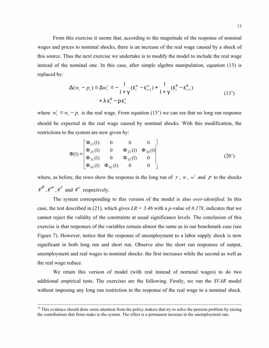
We retain this version of model (with real instead of nominal wages) to do two

additional empirical tests. The exercises are the following. Firstly, we run the SVAR model

without imposing any long run restriction in the response of the real wage to a nominal shock.

19 This evidence should draw some attention from the policy makers that try to solve the pension problem by raising the contributions that firms make to the system. The effect is a permanent increase in the unemployment rate.

14

Secondly, after reestablishing the version of the model with the real wage, we run the SVAR

without imposing long run restrictions of nominal shocks on the unemployment rate.

The evidence of these exercises suggests that nominal shocks, of the nature though for

this empirical model, does not have any effect on the real wage in the long run but a short term

response is captured by the model (see Figure 8).

Interestingly, for the second exercise, a nominal shock has the effect of reducing the

unemployment rate in the short run. In this version of the model output also reacts in the short

run while the real wage moves downward. Notice, however, that these effects last only about

one year then the responses are not significant (see Figure 9). These reactions of the variables

are fully consistent with backwards-formed expectations by the Colombian agents as it is

sometimes argued.

Now, let us think about an economy where a negative nominal shift announced every

year and made effective by the monetary authority but not believed by agents. The result is a

negative response of output and an increase in unemployment and the real wage in the short run.

No long run effect on any of these variables is possible according to our results. However, this

lack of credibility of monetary policy made feasible this joint behavior of the variables (and

agents) in the last years of the 1990s. Thus, to get a better performance of the economy, the

announcements of the monetary authority should be credible. If policy announcements had been

believed and taken into account when setting wages, unemployment had only increased because

of the impact of labor supply and non- wage labor costs.

As it might be obvious, these two last exercises would not be necessary since the long

run restrictions have not been rejected according to the statistics. However, some analysts of the

Colombian economy insist on a more active monetary policy to take the economy out of the

recession. Accordingly, these results suggest that the economy would have only a short run

reaction in output, unemployment and real wages. The cost of this behavior is to have a higher

price level both in short and long run (Figure 9). Of course if we assume that agents form

expectations rationally this policy could be undertaken only once, but if agents form

expectations backwards there is room for “managing the demand” over a few periods at a cost of

higher inflation.

15

6. Final remarks

In this work we present a small model for the Colombian economy with the aim of

understanding some of the possible causes of the deepest recession the country underwent

during the last fifty years. The model consists of structural equations for the product and labor

markets and some other definitions and assumptions. By using a non-triangular SVAR empirical

approach and quarterly data form 1984 up to 2000 we obtain sensible impulse response

functions for output, unemployment, and prices but less satisfactory for both nominal and real

wages. The result of the tests suggest that the long run restrictions, implied by the model, on the

response of the variables to productivity, nominal, labor supply, and non-wage labor costs

shocks can be imposed.

The evidence suggests that among the causes of the recession, the lack of credibility of

monetary policy seem to have a privileged place. Other shocks such as the labor supply and

non-wages labor costs also explain the increase in the unemployment rate. Most tellingly, the

exercise also shows the long run neutrality of nominal shocks to both output and unemployment.

However, these variables react in the short run to shocks of the same source.

Now, it is time for the authorities to analyze the way in which agents form their

expectations to exploit differences between expected and observed inflation or not given the

reaction in prices produced by these types of policies.

References

Algan, Y. (2002) How well does the aggregate demand-aggregate supply framework explain unemployment fluctuations? A France-United States comparison.. Economic Modelling, 19, 153-177. Amisano, G. and Giannini C. (1997) Topics in Structural VAR Econometrics. Springer-Verlag, Berlin. 2nd edition. Arango, L. E. (1998) Temporary and permanent components of Colombia’s output. Borradores de Economía, No. 96, Banco de la República. Arango, L.E. and Posada, C.E. (2001) El desempleo en Colombia, Coyuntura Social No. 24, 65-85.

16

Arango, L.E. and Posada, C.E. (2002) Unemployment rate and the real wage behaviour: a neoclassical hint for the Colombian labour market adjustment, Applied Economic Letters, 9, 425-428. Balmaseda, M.; Dolado, J. and López-Salido, J.D. (2000) The dynamic effects of shocks to labour markets: evidence from OECD countries. Oxford Economic Papers 52, 3-23. Blanchard, O. and Quah, D. (1989) The dynamic effects of aggregate demand and supply disturbances, The American Economic Review, Vol. 79, No. 4, 655-673. Blanchard, O. and Summers, L. (1986) Hysteresis in unemployment, European Economic Review, 31, 288-295. Cárdenas, M. and C. Gutiérrez (1998) Determinantes del desempleo en Colombia, Coyuntura Social, Debates. Situación y perspectivas del empleo y estrategias para su reactivación, Fedesarrollo, 9, 8-25. Dolado, J. and Jimeno, J. (1997) The causes of Spanish unemployment: A structural VAR approach, European Economic Review, 41, 1281-1307. Fabiani, S., Locarno, A., Oneto, G.P., and Sestito, P. (2001) The sources of unemployment fluctuations: an empirical application to the Italian case, Labour Economics, 8, 259-289. Hernández, A. and Tolosa , J. (2001) La política monetaria en Colombia en la segunda mitad de los años noventa, Borradores de Economía, No. 172. Banco de la República. Iregui, A.M and Otero, J. (2002) On the dynamics of unemployment in a developing economy: Colombia, Borradores de Economía No. 208, Banco de la República. Misas, M. and López, E. (1998) El producto potencial en Colombia: Una estimación bajo VAR estructural. Borradores de Economía, No. 94, Banco de la República. Misas, M. and López, E. (2001) Desequilibrios reales en Colombia. Ensayos sobre Política Económica, No. 40. Misas, M. and Posada, C. E. (2000) Crecimiento y ciclos económicos en Colombia en el siglo XX: el aporte de un VAR estructural. Borradores de Economía No.155, May. Restrepo, J. E. (1997) Modelo IS-LM para Colombia: Relaciones de largo plazo y fluctuaciones económicas. Archivos de Economía, No. 65. Sargent, T. and Wallace, N. (1975) Rational expectations, the optimal monetary instrument and the optimal policy rule, Journal of Political Economy, 83, 241-54. Urrutia, M. (2002) Una visión alternativa: la política monetaria y cambiaria en la última década, Revista Banco de la República, Vol. LXXV No. 895.

17

Appendix 1: Diagnostics tests for the residuals of the reduced-form VAR For system with nominal wages

Value p-value

Jarque-Bera 8.64 0.37

Adjusted-Q statistic1/ 248.78 0.03

Serial correlation LM test1/ 26.45 0.05 1/ Evaluated up to 15 lags. Note: these statistics correspond to the system graphed in Figure 6.

For system with real wages

Value p-value Jarque-Bera 10.72 0.22

Adjusted-Q statistic1/ 229.40 0.15

Serial correlation LM test1/ 16.60 0.41 1/ Evaluated up to 15 lags. Note: these statistics correspond to the system graphed in Figure 7.

Appendix 2: Identification of a structural VAR with long-run constrains

Amisano and Giannini (1997) show that the identification of the model, including the

restrictions in (21), can be analyzed in terms of the following systems of equations:

[ ]0=yNk (A.1)

( ) [ ]00 =⊗ yIR φ (A.2)

The system (A.1) has 2k equations in 2k unknowns and the system (A.2) has n

equations in 2k unknowns. The two systems are connected because they share the same 2k unknowns.

Amisano and Giannini(1997) suggest to insert the general solution of (A1) in (A2). The

vector representing the general solution of system (A1) can be written as:

xDy k~= (A.3)

18

where x is a k(k-1)/2 vector of free elements, kD~ is a k2×k(k-1)/2 full column rank matrix which

columns are associated with the eigenvectors corresponding to the zero eigenvalues of the Nk

matrix with ( )kkkk IN ⊕+= 221 and kk⊕ is the commutation matrix20 of dimensions k2×k2.

Inserting (A.3) in the system (A2) we obtain:

[ ]0~)( 0 =⊗ xDIR kφ (A.4)

Therefore, the system is identified if and only if (A.4) with the matrix kDIR ~)( 0φ⊗

evaluated at *0φ has only admissible solution [ ]0=x . In order to evaluate the identification of our

model, we need to define the matrices R and kD~ .

Computation of the R matrix

The R matrix is associated to the restrictions that are imposed to the reduced-form shocks. For

the model with real wage, we have the following long-run constraints:

ΦΦΦΦ

ΦΦΦΦ

=Φ

00)1()1(0)1(0)1(

)1()1(0)1(000)1(

)1(

4241

3331

242321

11

(A.5)

From equations (17), (18) and (19) it is straightforward to obtain the relationship:

0)1()1( φC=Φ (A.6)

Then, using (A.6) the restrictions implied in (A5) can be noted as:

dR =)( 0φvec (A.7)

Specifically (A.6) implies:

Then, the long-run constrains of the previous expression imply the following equations:

20 Let A be a p×q matrix. The vectors vec(A) and vec(A’) clearly contain the same pq components, but in different order. Hence, there exists a unique pq×pq permutation matrix which transforms vec(A) into vec(A’). This matrix is called the commutation matrix and is denoted ⊕ . Thus: )()( AvecAvecpq ′=⊕ .

19

0)1()1()1()1(0)1()1()1()1(0)1()1()1()1(0)1()1()1()1(0)1()1()1()1(

0)1()1()1()1(0)1()1()1()1(0)1()1()1()1(

44,04434,04324,04214,041

43,04433,04323,04213,041

44,03434,03324,03214,031

42,03432,03322,03212,031

42,02432,02322,02212,021

44,01434,01324,01214,011

43,01433,01323,01213,011

42,01432,01322,01212,011

=+++=+++=+++=+++=+++=+++=+++=+++

φφφφφφφφφφφφφφφφφφφφφφφφφφφφφφφφ

CCCCCCCCCCCCCCCCCCCCCCCCCCCCCCCC

These eight equations can be expressed in the notation of (A.7) with d as a vector of

zeros and the following R matrix:

=

)1()1()1()1(0000000000000000)1()1()1()1(00000000

)1()1()1()1(00000000000000000000)1()1()1()1(000000000000)1()1()1()1(0000

)1()1()1()1(0000000000000000)1()1()1()1(0000000000000000)1()1()1()1(0000

44434241

44434241

34333231

34333231

24232221

14131211

14131211

14131211

CCCCCCCC

CCCCCCCCCCCC

CCCCCCCC

CCCC

R

The components of the R matrix can be easily estimated since they come from the

reduced-form VAR.21

Computation of the matrix kD~

As stated above, the columns of kD~ are associated with the eigenvectors that correspond to zero

eigenvalues of the Nk matrix with ( )kkkk IN ⊕+= 221 and kk⊕ as the commutation matrix. For

our case k=4, hence the commutation matrix 44⊕ is:

21 The fact that the R matrix involves non-constant terms but the reduced form cumulated impulse response functions coefficients, C(1), which are not known and must be estimated causes some complications in the SVAR analysis. However, Amisano and Giannini (1997) show that under this situation we still can have consistent estimators for the optimization process.

20

=⊕

1000000000000000000010000000000000000000100000000000000000001000010000000000000000000100000000000000000001000000000000000000010000100000000000000000001000000000000000000010000000000000000000100001000000000000000000010000000000000000000100000000000000000001

44

And the 4~D matrix is the following:

−−

−

−−

−

=

000000010000000010000100010000000000

100000001000000010100000000000000001000100001000000001000000

~4D

With the previous definitions of R and 4~D and using some algebra it is easy to prove that

for any vector x, of dimension 6×1, the system [ ]0~)( *0

=⊗ xDIR kφ has only the admissible

solution [ ]0=x . Then, given the result of the order condition, number of restrictions greater than

k(k-1)/2, our system (with real wage) is over-identified.

Figure 6. Impulse response functions with nominal wages in the system

To a productivity shock To a nominal shock To a labor supply shock To a labor cost shock

Response

of

output

0.00000

0.00500

0.01000

0.01500

0.02000

0.02500

0.03000

1 3 5 7 9 11 13 15 17 19 21 23 25 27 29 31 33 35 37 39

-0.00800

-0.00600

-0.00400

-0.00200

0.00000

0.00200

0.00400

0.00600

0.00800

0.01000

0.01200

1 3 5 7 9 11 13 15 17 19 21 23 25 27 29 31 33 35 37 39

-0.00600

-0.00400

-0.00200

0.00000

0.00200

0.00400

0.00600

0.00800

0.01000

1 3 5 7 9 11 13 15 17 19 21 23 25 27 29 31 33 35 37 39

-0.00800

-0.00600

-0.00400

-0.00200

0.00000

0.00200

0.00400

0.00600

0.00800

1 3 5 7 9 11 13 15 17 19 21 23 25 27 29 31 33 35 37 39

Response

of

unemployment

-0.00450

-0.00400

-0.00350

-0.00300

-0.00250

-0.00200

-0.00150

-0.00100

-0.00050

0.000001 3 5 7 9 11 13 15 17 19 21 23 25 27 29 31 33 35 37 39

-0.00250

-0.00200

-0.00150

-0.00100

-0.00050

0.00000

0.00050

0.00100

0.00150

0.00200

0.00250

1 3 5 7 9 11 13 15 17 19 21 23 25 27 29 31 33 35 37 39

-0.00150

-0.00100

-0.00050

0.00000

0.00050

0.00100

0.00150

0.00200

0.00250

0.00300

1 3 5 7 9 11 13 15 17 19 21 23 25 27 29 31 33 35 37 39

0.00000

0.00100

0.00200

0.00300

0.00400

0.00500

0.00600

0.00700

0.00800

1 3 5 7 9 11 13 15 17 19 21 23 25 27 29 31 33 35 37 39

Response

of

nominal wage

-0.01000

-0.00500

0.00000

0.00500

0.01000

0.01500

1 3 5 7 9 11 13 15 17 19 21 23 25 27 29 31 33 35 37 39

0.00000

0.00500

0.01000

0.01500

0.02000

0.02500

0.03000

0.03500

0.04000

0.04500

0.05000

1 3 5 7 9 11 13 15 17 19 21 23 25 27 29 31 33 35 37 39

0.00000

0.00500

0.01000

0.01500

0.02000

0.02500

0.03000

0.03500

1 3 5 7 9 11 13 15 17 19 21 23 25 27 29 31 33 35 37 39

-0.01500

-0.01000

-0.00500

0.00000

0.00500

0.01000

0.01500

1 3 5 7 9 11 13 15 17 19 21 23 25 27 29 31 33 35 37 39

Response

of

prices

-0.01000

-0.00800

-0.00600

-0.00400

-0.00200

0.00000

0.00200

0.00400

0.00600

0.00800

1 3 5 7 9 11 13 15 17 19 21 23 25 27 29 31 33 35 37 39

0.00000

0.00500

0.01000

0.01500

0.02000

0.02500

0.03000

0.03500

0.04000

1 3 5 7 9 11 13 15 17 19 21 23 25 27 29 31 33 35 37 39

-0.01000

-0.00800

-0.00600

-0.00400

-0.00200

0.00000

0.00200

0.00400

0.00600

0.00800

0.01000

1 3 5 7 9 11 13 15 17 19 21 23 25 27 29 31 33 35 37 39

-0.00800

-0.00600

-0.00400

-0.00200

0.00000

0.00200

0.00400

0.00600

0.00800

0.01000

1 3 5 7 9 11 13 15 17 19 21 23 25 27 29 31 33 35 37 39

22

Figure 7. Impulse response functions with real wages in the system

To a productivity shock To a nominal shock To a labor supply shock To a labor cost shock

Response

of

output

0.00000

0.00500

0.01000

0.01500

0.02000

0.02500

0.03000

1 3 5 7 9 11 13 15 17 19 21 23 25 27 29 31 33 35 37 39

-0.01000

-0.00500

0.00000

0.00500

0.01000

0.01500

1 3 5 7 9 11 13 15 17 19 21 23 25 27 29 31 33 35 37 39

-0.00800

-0.00600

-0.00400

-0.00200

0.00000

0.00200

0.00400

0.00600

1 3 5 7 9 11 13 15 17 19 21 23 25 27 29 31 33 35 37 39

-0.00800

-0.00600

-0.00400

-0.00200

0.00000

0.00200

0.00400

0.00600

0.00800

1 3 5 7 9 11 13 15 17 19 21 23 25 27 29 31 33 35 37 39

Response

of

unemployment

-0.00450

-0.00400

-0.00350

-0.00300

-0.00250

-0.00200

-0.00150

-0.00100

-0.00050

0.000001 3 5 7 9 11 13 15 17 19 21 23 25 27 29 31 33 35 37 39

-0.00250

-0.00200

-0.00150

-0.00100

-0.00050

0.00000

0.00050

0.00100

0.00150

0.00200

0.00250

1 3 5 7 9 11 13 15 17 19 21 23 25 27 29 31 33 35 37 39

-0.00050

0.00000

0.00050

0.00100

0.00150

0.00200

0.00250

0.00300

0.00350

1 3 5 7 9 11 13 15 17 19 21 23 25 27 29 31 33 35 37 39

0.00000

0.00100

0.00200

0.00300

0.00400

0.00500

0.00600

0.00700

0.00800

1 3 5 7 9 11 13 15 17 19 21 23 25 27 29 31 33 35 37 39

Response

of

real wage

-0.01500

-0.01000

-0.00500

0.00000

0.00500

0.01000

1 3 5 7 9 11 13 15 17 19 21 23 25 27 29 31 33 35 37 39

-0.01500

-0.01000

-0.00500

0.00000

0.00500

0.01000

0.01500

1 3 5 7 9 11 13 15 17 19 21 23 25 27 29 31 33 35 37 39

0.00000

0.00500

0.01000

0.01500

0.02000

0.02500

0.03000

0.03500

0.04000

1 3 5 7 9 11 13 15 17 19 21 23 25 27 29 31 33 35 37 39

-0.01000

-0.00800

-0.00600

-0.00400

-0.00200

0.00000

0.00200

0.00400

0.00600

0.00800

0.01000

1 3 5 7 9 11 13 15 17 19 21 23 25 27 29 31 33 35 37 39

Response

of

prices

-0.01200

-0.01000

-0.00800

-0.00600

-0.00400

-0.00200

0.00000

0.00200

0.00400

0.00600

1 3 5 7 9 11 13 15 17 19 21 23 25 27 29 31 33 35 37 39

0.00000

0.00500

0.01000

0.01500

0.02000

0.02500

0.03000

0.03500

1 3 5 7 9 11 13 15 17 19 21 23 25 27 29 31 33 35 37 39

-0.00800

-0.00600

-0.00400

-0.00200

0.00000

0.00200

0.00400

0.00600

0.00800

0.01000

1 3 5 7 9 11 13 15 17 19 21 23 25 27 29 31 33 35 37 39

-0.00800

-0.00600

-0.00400

-0.00200

0.00000

0.00200

0.00400

0.00600

0.00800

0.01000

1 3 5 7 9 11 13 15 17 19 21 23 25 27 29 31 33 35 37 39

23

Figure 8. Impulse response functions with real wages in the system but

without long run restrictions on real wages to a nominal shock. To a productivity shock To a nominal shock To a labor supply shock To a labor cost shock

Response

of

output

0.00000

0.00500

0.01000

0.01500

0.02000

0.02500

0.03000

1 3 5 7 9 11 13 15 17 19 21 23 25 27 29 31 33 35 37 39

-0.01000

-0.00500

0.00000

0.00500

0.01000

0.01500

1 3 5 7 9 11 13 15 17 19 21 23 25 27 29 31 33 35 37 39

-0.00800

-0.00600

-0.00400

-0.00200

0.00000

0.00200

0.00400

0.00600

1 3 5 7 9 11 13 15 17 19 21 23 25 27 29 31 33 35 37 39

-0.00800

-0.00600

-0.00400

-0.00200

0.00000

0.00200

0.00400

0.00600

0.00800

1 3 5 7 9 11 13 15 17 19 21 23 25 27 29 31 33 35 37 39

Response

of

unemployment

-0.00450

-0.00400

-0.00350

-0.00300

-0.00250

-0.00200

-0.00150

-0.00100

-0.00050

0.000001 3 5 7 9 11 13 15 17 19 21 23 25 27 29 31 33 35 37 39

-0.00250

-0.00200

-0.00150

-0.00100

-0.00050

0.00000

0.00050

0.00100

0.00150

0.00200

0.00250

1 3 5 7 9 11 13 15 17 19 21 23 25 27 29 31 33 35 37 39

-0.00050

0.00000

0.00050

0.00100

0.00150

0.00200

0.00250

0.00300

0.00350

0.00400

1 3 5 7 9 11 13 15 17 19 21 23 25 27 29 31 33 35 37 39

0.00000

0.00100

0.00200

0.00300

0.00400

0.00500

0.00600

0.00700

0.00800

1 3 5 7 9 11 13 15 17 19 21 23 25 27 29 31 33 35 37 39

Response

of

real wage

-0.01200

-0.01000

-0.00800

-0.00600

-0.00400

-0.00200

0.00000

0.00200

0.00400

0.00600

0.00800

1 3 5 7 9 11 13 15 17 19 21 23 25 27 29 31 33 35 37 39

-0.01000

-0.00500

0.00000

0.00500

0.01000

0.01500

1 3 5 7 9 11 13 15 17 19 21 23 25 27 29 31 33 35 37 39

0.00000

0.00500

0.01000

0.01500

0.02000

0.02500

0.03000

0.03500

0.04000

1 3 5 7 9 11 13 15 17 19 21 23 25 27 29 31 33 35 37 39

-0.01000

-0.00800

-0.00600

-0.00400

-0.00200

0.00000

0.00200

0.00400

0.00600

0.00800

0.01000

1 3 5 7 9 11 13 15 17 19 21 23 25 27 29 31 33 35 37 39

Response

of

prices

-0.01200

-0.01000

-0.00800

-0.00600

-0.00400

-0.00200

0.00000

0.00200

0.00400

0.00600

1 3 5 7 9 11 13 15 17 19 21 23 25 27 29 31 33 35 37 39

0.00000

0.00500

0.01000

0.01500

0.02000

0.02500

0.03000

0.03500

1 3 5 7 9 11 13 15 17 19 21 23 25 27 29 31 33 35 37 39

-0.00800

-0.00600

-0.00400

-0.00200

0.00000

0.00200

0.00400

0.00600

0.00800

0.01000

1 3 5 7 9 11 13 15 17 19 21 23 25 27 29 31 33 35 37 39

-0.00800

-0.00600

-0.00400

-0.00200

0.00000

0.00200

0.00400

0.00600

0.00800

0.01000

1 3 5 7 9 11 13 15 17 19 21 23 25 27 29 31 33 35 37 39

24

Figure 9. Impulse response functions with real wages in the system but without long run restrictions on unemployment to a nominal shock.

To a productivity shock To a nominal shock To a labor supply shock To a labor cost shock

Response

of

output

0.00000

0.00500

0.01000

0.01500

0.02000

0.02500

0.03000

1 3 5 7 9 11 13 15 17 19 21 23 25 27 29 31 33 35 37 39

-0.01000

-0.00500

0.00000

0.00500

0.01000

0.01500

1 3 5 7 9 11 13 15 17 19 21 23 25 27 29 31 33 35 37 39

-0.00800

-0.00600

-0.00400

-0.00200

0.00000

0.00200

0.00400

0.00600

1 3 5 7 9 11 13 15 17 19 21 23 25 27 29 31 33 35 37 39

-0.00800

-0.00600

-0.00400

-0.00200

0.00000

0.00200

0.00400

0.00600

0.00800

1 3 5 7 9 11 13 15 17 19 21 23 25 27 29 31 33 35 37 39

Response

of unemployment

-0.00450

-0.00400

-0.00350

-0.00300

-0.00250

-0.00200

-0.00150

-0.00100

-0.00050

0.000001 3 5 7 9 11 13 15 17 19 21 23 25 27 29 31 33 35 37 39

-0.00350

-0.00300

-0.00250

-0.00200

-0.00150

-0.00100

-0.00050

0.00000

0.00050

0.00100

0.00150

1 3 5 7 9 11 13 15 17 19 21 23 25 27 29 31 33 35 37 39

-0.00050

0.00000

0.00050

0.00100

0.00150

0.00200

0.00250

0.00300

0.00350

0.00400

1 3 5 7 9 11 13 15 17 19 21 23 25 27 29 31 33 35 37 39

0.00000

0.00100

0.00200

0.00300

0.00400

0.00500

0.00600

0.00700

0.00800

1 3 5 7 9 11 13 15 17 19 21 23 25 27 29 31 33 35 37 39

Response

of

real wage

-0.01200

-0.01000

-0.00800

-0.00600

-0.00400

-0.00200

0.00000

0.00200

0.00400

0.00600

0.00800

0.01000

1 3 5 7 9 11 13 15 17 19 21 23 25 27 29 31 33 35 37 39

-0.01500

-0.01000

-0.00500

0.00000

0.00500

0.01000

0.01500

1 3 5 7 9 11 13 15 17 19 21 23 25 27 29 31 33 35 37 39

0.00000

0.00500

0.01000

0.01500

0.02000

0.02500

0.03000

0.03500

0.04000

1 3 5 7 9 11 13 15 17 19 21 23 25 27 29 31 33 35 37 39

-0.01000

-0.00800

-0.00600

-0.00400

-0.00200

0.00000

0.00200

0.00400

0.00600

0.00800

1 3 5 7 9 11 13 15 17 19 21 23 25 27 29 31 33 35 37 39

Response

of

prices

-0.01200

-0.01000

-0.00800

-0.00600

-0.00400

-0.00200

0.00000

0.00200

0.00400

0.00600

1 3 5 7 9 11 13 15 17 19 21 23 25 27 29 31 33 35 37 39

0.00000

0.00500

0.01000

0.01500

0.02000

0.02500

0.03000

0.03500

1 3 5 7 9 11 13 15 17 19 21 23 25 27 29 31 33 35 37 39

-0.00800

-0.00600

-0.00400

-0.00200

0.00000

0.00200

0.00400

0.00600

0.00800

0.01000

1 3 5 7 9 11 13 15 17 19 21 23 25 27 29 31 33 35 37 39

-0.00800

-0.00600

-0.00400

-0.00200

0.00000

0.00200

0.00400

0.00600

0.00800

0.01000

1 3 5 7 9 11 13 15 17 19 21 23 25 27 29 31 33 35 37 39