Embed Size (px)
Citation preview
Reconstructing Reticulate Evolution in Species – Theoryand Practice
Luay NakhlehDepartment of Computer
SciencesUniversity of Texas at Austin
Austin, Texas [email protected]
Tandy Warnow∗
Department of ComputerSciences
University of Texas at AustinAustin, Texas 78712
C. Randal LinderSection of Integrative BiologySchool of Biological SciencesUniversity of Texas at Austin
Austin, Texas [email protected]
ABSTRACTWe present new methods for reconstructing reticulate evo-lution of species due to events such as horizontal transferor hybrid speciation; both methods are based upon exten-sions of Wayne Maddison’s approach in his seminal 1997paper. Our first method is a polynomial time algorithmfor constructing phylogenetic networks from two gene treescontained inside the network. We allow the network to havean arbitrary number of reticulations, but we limit the retic-ulation in the network so that the cycles in network arenode-disjoint (“galled”); we prove accuracy guarantees forour first method by presenting a formal characterization ofthe set of gene trees defined by a species network. Our sec-ond method is a polynomial time algorithm for constructingnetworks with one reticulation, where we allow for errors inthe estimated gene trees. Using simulations, we demonstrateimproved performance of this method over both Neighbor-Net and Maddison’s method.
Categories and Subject DescriptorsF.2.0 [Theory of Computation]: General; G.4 [Mathem-atical Software]: Algorithm Design and Analysis; J.3 [Co-mputer Applications]: Life and Medical Sciences
General TermsAlgorithms, Theory, Experimentation.
KeywordsPhylogenetic networks, gene trees, subtree prune and re-graft.
∗Currently on sabbatical at the Radcliffe Institute for Ad-vanced Study.
Permission to make digital or hard copies of all or part of this work forpersonal or classroom use is granted without fee provided that copies arenot made or distributed for profit or commercial advantage and that copiesbear this notice and the full citation on the first page. To copy otherwise, torepublish, to post on servers or to redistribute to lists, requires prior specificpermission and/or a fee.RECOMB’04, March 27–31, 2004, San Diego, California, USA.Copyright 2004 ACM 1-58113-755-9/04/0003 ...$5.00.
1. INTRODUCTIONThe motivation for this paper is the problem of recon-
structing accurate evolutionary history in the presence ofreticulation events, such as hybrid speciation (where organ-isms hybridize and create new species), or horizontal trans-fer (via hybridization or viral transmission, for example).Both types of reticulation events are sufficiently commonto be of serious concern to systematists; hybrid speciationis common in some very large groups of organisms: plants,fish, amphibians, and many lineages of invertebrates, andhorizontal gene transfer appears to be very common in bac-teria [8] with lower levels being evident in many multicel-lular groups. Such evolutionary histories cannot be ade-quately represented using trees; instead, phylogenetic net-works (which are basically directed acyclic graphs, coupledwith time constraints) are used.
Several methods exist for reconstructing phylogenetic net-works from gene datasets; of these, NeighborNet by Bryantand Moulton [2] and a method by Wayne Maddison [10]are the most relevant to this paper. NeighborNet uses a“combined analysis” approach because it combines sequencedatasets by concatenation, and then seeks the phylogeneticnetwork on the basis of the distance matrix produced bythe combined dataset. Maddison, on the other hand, uses aseparate analysis where the network can be reconstructedby first inferring individual gene trees from separate se-quence datasets, and then reconciling the trees into a net-work. Maddison also showed the connection between phylo-genetic network reconstruction and the calculation of rootedsubtree prune and regraft (rSPR) distances (which we de-fine and discuss below). Maddison showed explicitly how toconstruct a network containing a single reticulation from itstwo trees (which are related by one rSPR move), and sug-gested that networks with additional reticulations could beinferred from individual gene trees, provided that the rSPRdistance between two constituent gene trees could be calcu-lated. However, Maddison did not show (or prove) how touse rSPR distance calculations in order to construct phylo-genetic networks. Furthermore, the rSPR Distance problemis currently of unknown complexity [1] (a naıve algorithmwould solve the problem in O(n2m) time, where n is thenumber of leaves in each of the trees, and m is the rSPRdistance between the trees).
In this paper we consider the inference of “gt-networks”(for “galled tree” networks, which is the terminology usedin [6]); these are phylogenetic networks in which reticula-
tion events are constrained so as to be evolutionarily inde-pendent of each other (see [6] for a biological justificationof the model). This model was first introduced by Wang etal. [15], and later formalized and further pursued by Gus-field et al. [6]. For this special case, we present polynomialtime algorithms that provably reconstruct accurate phylo-genetic networks, provided that accurate gene trees can beobtained. We also present polynomial time algorithms forreconstructing phylogenetic networks from inaccurate genetrees, and we demonstrate the improvement in accuracy ofthese methods over two previous methods for phylogeneticnetwork reconstruction in simulation.
The rest of the paper is organized as follows. In Section 2we briefly describe phylogenetic networks, including the def-inition of gt-networks and the rSPR operation. In Section 3,we briefly describe two of the evolutionary events that neces-sitate the use of phylogenetic networks; we also review Mad-dison’s approach and discuss its limitations. In Section 4 wepresent a formal characterization of gene trees within speciesnetworks in terms of the rSPR distances among them, andthen present our efficient algorithm for reconciling accurategene trees into a gt-network. In Section 5, we present alinear time algorithm for the following nice combinatorialproblem: given two trees t1 and t2, does there exist a pairof trees T1 and T2 refining t1 and t2, respectively, such thatT1 and T2 are the two induced trees in a gt-network withone reticulation? We show how to use this algorithm for re-constructing phylogenetic networks in practice in Section 6,and we (briefly) summarize the results of a simulation studycomparing the performance of this method (which we callSpNet, for “Species Network”) to NeighborNet. We closein Section 7 with final remarks and directions for future re-search.
2. NETWORKS AND GT-NETWORKS
2.1 Background
2.1.1 Graph-theoretic definitionsGiven a (directed) graph G, E(G) denotes the set of (di-
rected) edges of G and V (G) denotes the set of nodes of G.We write (u, v) to denote a directed edge from node u tonode v, in which case u is the tail, v the head of the edge,and u is a parent of v. The indegree of a node v is the num-ber of edges whose head is v, while the outdegree of v is thenumber of edges whose tail is v. A directed path of lengthk from u to v in G is a sequence u0u1 · · ·uk of nodes withu = u0, v = uk, and ∀i, 1 ≤ i ≤ k, (ui−1, ui) ∈ E(G); wesay that u is the tail of p and v is the head of p.
Node v is reachable from u in G, denoted u ; v, if thereis a directed path in G from u to v; we then also say thatu is an ancestor of v. Given a tree T and a subset L′ ofthe leaves, we write T |L′ to denote the subtree obtained byrestricting T to leaves L′, i.e., by removing all leaves not inL′ and all incident edges. If X is a subtree of T , we denoteby T \ X the tree obtained by removing subtree X from T .
We denote by L(T ) the leaf-set of a tree T . An undirectedpath p of length k between u and v in a rooted tree T is asequence u0u1 · · ·uk of nodes with u = u0, v = uk, and∀i, 1 ≤ i ≤ k, either (ui−1, ui) or (ui, ui−1) is an edge ofT . If p is an undirected path in tree T , and whose twoendpoints are u and v, we denote by END(p) = (U,V ) thetwo subtrees U and V attached to u and v, respectively, and
that do not contain any edges from p. We use p to denotethe path itself, as well as the edges of the path.
2.1.2 Strict consensus and compatibility treesLet T be a tree leaf-labeled by a set S of taxa. Each edge
e in T induces a bipartition π(e) = {A(e)|B(e)} on the set S,where A(e) is the set of taxa “below” e, and B(e) is the setcontaining the rest of the taxa. We denote by C(T ) the setof all bipartitions induced by tree T . We say that e1 and e2
(and their associated bipartitions) are compatible, denotede1 ≡ e2, if there exists a tree T that induces both π(e1) andπ(e2). This definition of compatibility naturally extends tosets of bipartitions, and hence also to trees.
If we contract an edge in T , thus identifying the endpointsof that edge, we obtain another tree T ′ on the same leaf set;T is then said to refine T ′, and T ′ is said to be a contractionof T . If T ′′ is the result of contracting a set of edges in T ,then too T ′′ is a contraction of T , and T is a refinement ofT ′′.
A set of trees is compatible if the trees have a commonrefinement; its minimal common refinement (called the com-patibility tree) is unique. For any set of trees, the maximallyresolved common contraction (called the strict consensustree) is also unique. Both the compatibility and strict con-sensus trees can be found in O(kn) time, where there are ktrees on the same set of n leaves [5, 16, 3].
Given two trees T1 and T2, the set U(T1, T2) contains alledges of T1 that are not compatible with T2; U(T2, T1) isdefined similarly. Note then that T1 and T2 are compatibleif U(T1, T2) = U(T2, T1) = ∅.
If a tree T has a node v with indegree and outdegree one,we replace the two edges incident to v by a single edge; thisoperation on T is called forced contraction.
2.2 Phylogenetic networksA phylogenetic network N = (V, E) with a set L ⊆ V of
n leaves, is a directed acyclic graph in which exactly onenode has no incoming edges (the root), and all other nodeshave either one incoming edge (tree nodes) or two incomingedges (reticulation nodes). The nodes in L have no outgoingedges. Tree edges are those whose head is a tree node, andnetwork edges are those whose head is a reticulation node.
In this paper, we focus on binary networks, i.e., networksin which the outdegree of a reticulation node is 1 and theoutdegree of a tree node is 2. Further, all trees are binary,i.e., all nodes (except for the leaves) have outdegree 2.
As discussed in [9], reticulation events impose time con-straints on the phylogenetic network, which we now brieflyreview. A phylogenetic network N = (V, E) defines a partialorder on the set V of nodes. Based on this partial order, weassign times to the nodes of N , associating time t(u) withnode u. If there is a directed path p from node u to nodev, such that p contains at least one tree edge, then we musthave t(u) < t(v) (in order to respect the time flow). Ife = (u, v) is a network edge, then we must have t(u) = t(v)(because a reticulation event is, at the scale of evolution, aninstantaneous process).
Given a network N , we say that p is a positive-time di-rected path from u to v, if p is a directed path from u tov, and p contains at least one tree edge. Given a networkN , two nodes u and v cannot co-exist in time if there existsa sequence P = 〈p1, p2, . . . , pk〉 of paths such that (1) pi isa positive-time directed path, for every 1 ≤ i ≤ k, (2) u
is the tail of p1, and v is the head of pk, and (3) for every1 ≤ i ≤ k − 1, there exists a reticulation node whose twoparents are the head of pi and the tail of pi+1.
If two nodes u and v cannot co-exist in time, then theycannot be “involved” in a reticulation event. In other words,u and v cannot be the two parents of a hybrid (i.e., theredoes not exist a reticulation node w such that (u, w) and(v, w) are edges in the network), nor can there be a horizon-tal gene transfer between them (i.e., neither (u, v) nor (v, u)can be an edge in the network). This property is furtherdiscussed in [10, 12, 9].
2.3 gt-NetworksIn this paper, we assume a biologically-motivated restricted
class of phylogenetic networks, called gt-networks, proposedby Wang et al. [15] and Gusfield et al. [6].
Definition 1. In a phylogenetic network N , let w be anode that has two directed paths out of it that meet at areticulation node x. Those two directed paths together definea “reticulation cycle” Q. Node w is called the “coalescentnode” of Q, and x is the “reticulation node” of Q.
Definition 2. A reticulation cycle in a phylogenetic net-work that shares no nodes with any other reticulation cycleis called a “gall”.
We denote by Qwx a gall whose coalescent node is w and
whose reticulation node is x. We denote by E(Qwx ) the set
of all edges on gall Q; formally, E(Qwx ) = {e : e is an edge
on a directed path from w to x}. The set RE(Qwx ) (for
“reticulation edges”) denotes the edges whose head is x, i.e.,the edges incident into x. When the context is clear, wesimply write Q for a gall, without explicitly naming thecoalescent and reticulation nodes.
Definition 3. A phylogenetic network N is called a “gt-network” if every reticulation cycle is a gall.
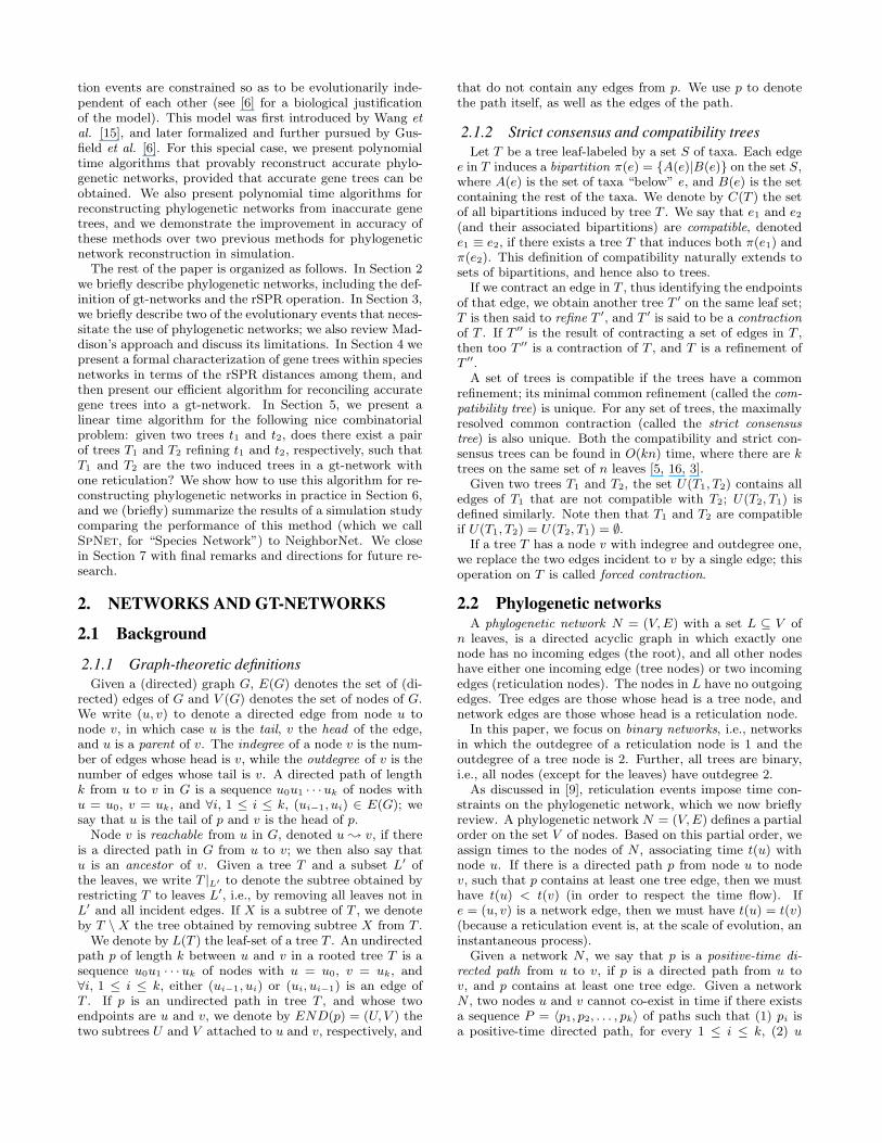
Figure 1(a) shows a gt-network N with a gall Qwx . The
set E(Qwx ) contains the edges (w, w1), (w1, u1), (w, w2),
(w2, u2), (u1, x), and (u2, x). The set RE(Qwx ) contains the
two edges (u1, x) and (u2, x). Obviously, gt-networks satisfythe synchronization property. In this paper, we assume thatthere is at least one tree node on each of the two paths fromw to x in a gall Qw
x (otherwise, the network would violatethe synchronization property).
We break a gall Qwx by removing exactly one of the edges
in the set RE(Qwx ).
Definition 4. A tree T is induced by a gt-network N ifT can be obtained from N through one of the possible waysof breaking all the galls in N , followed by forced contractionoperations on all nodes of indegree and outdegree 1.
Figures 1(b) and 1(c) show the two possible trees inducedby the gt-network N in Figure 1(a). To obtain the tree inFigure 1(b), the gall was broken by removing edge (u1, x)and applying forced contraction to node x; to obtain the treein Figure 1(c), the gall was broken by removing edge (u2, x)and applying forced contraction to node x. In general, givena network N with p reticulation nodes, we say that a tree Tis induced by N if T can be obtained by removing exactlyone of the two edges incoming into each of the p reticulationnodes in N .
Definition 5. Let Qwx be gall in a gt-network N , with
RE(Q) = {e1 = (u1, x), e2 = (u2, x)}. Further, let w1 bethe parent of u1, and w2 be the parent of u2. Assume treeT1 is obtained from N by removing edge e1, and tree T2
is obtained from N by removing edge e2. The two directedpaths w ; w1 and w ; u2 together define a “reticulationpath” in T1, and the two directed paths w ; w2 and w ; u1
together define a “reticulation path” in T2.
Given a gt-network with m galls, there are 2m possible waysof breaking the m galls, and thus inducing a tree. There isa direct correspondence between the edges and nodes of agt-network N and a tree T induced by N , and hence we talkabout a node or edge of T in N , or a node or edge of N inT (excluding the edges in RE(Q) and the nodes removed byforced contraction). We denote by RP Q(T ) the “reticulationpath” in T that results from breaking gall Q. The markededges in tree T1 of Figure 1(b) form the reticulation pathRP Q(T1), and the marked edges in tree T2 of Figure 1(c)form the reticulation path RP Q(T2) (we also use RP Q(T )to denote the edges on the reticulation path in T ).
2.4 The rSPR operationThe rSPR operation transforms rooted trees into other
rooted trees, and gene trees contained inside species net-works are related to each other by rSPR operations; we nowexplain this relationship. Observe that the two rooted treesT1 and T2 in Figures 1(b) and 1(c) (induced by the networkin Figure 1(a)) differ only in the location of the subtree T .Tree T2 can be obtained from T1 by “pruning” the subtreeT and “regrafting” it to another edge. In this case, we saythat T2 is obtained from T1 by one rooted subtree prune andregraft (rSPR) operation.
Definition 6. (From [1]) A rooted subtree prune andregraft (rSPR) on a rooted binary tree T is defined as cut-ting any edge and thereby pruning a subtree, t, and thenregrafting the subtree by the same cut edge to a new vertexobtained by subdividing a pre-existing edge in T −t. We alsoapply a forced contraction to maintain the binary propertyof the resulting tree.
The rSPR distance between two rooted binary trees T1 andT2, denoted by drSPR(T1, T2), is the minimum number ofrSPR operations needed to obtain T2 from T1. Computingthe rSPR distance between trees plays a central role in themethod that we propose for reconstructing networks. Weformally define the (decision) rSPR distance problem as fol-lows.
Definition 7. (The m-rSPR Distance Problem)
Input: Two binary trees, T1 and T2, leaf-labeled by a set Sof n taxa, and a nonnegative integer m.
Question: Is drSPR(T1, T2) = m?
The m-rSPR Distance Problem is of unknown computa-tional complexity [1]. However, for any constant m, we cansolve the m-rSPR Distance Problem in polynomial-time, aswe show in the following theorem.
Theorem 1. Given two binary trees T1 and T2 leaf-labeledby a set S of n leaves, and a constant m, we can decidewhether drSPR(T1, T2) = m in O(n2m) time.
w
T
u1 u2
w1 w2
X Y
x
w
T
w1
u2
X Y
w
T
u1
w2
X Y
(a) (b) (c)
Figure 1: (a) A gall Q whose coalescent and reticulation nodes are w and x respectively. (b) and (c) showthe two possible ways of “breaking” the gall Q to induce trees T1 and T2, respectively. The marked edges inT1 and T2 form RP Q(T1) and RP Q(T2), respectively.
The proof follows directly from Definition 6 and Theorem 2.1of [1], and is omitted. In this paper, we give an O(mn) al-gorithm for reconstructing a gt-network with m reticulationnodes from a pair of trees T1 and T2, each on n leaves.
3. RETICULATE EVOLUTIONA phylogeny of a set S of organisms is a graphical rep-
resentation of the evolution of S, typically a rooted binarytree, leaf-labelled by S. However, events such as hybrid spe-ciation and horizontal gene transfer require non-tree modelsfor accurate representations of evolution.
In what follows we will assume that the individual genedatasets are recombination-free (so that meiotic recombi-nation, or exchanges between sister chromosomes, does nottake place); this simplifies our analysis, and allows us to as-sume that all gene evolution is tree-like [4, 13, 17]. We alsoassume there are no gene gains or losses in the network.
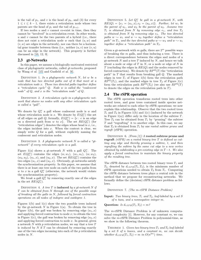
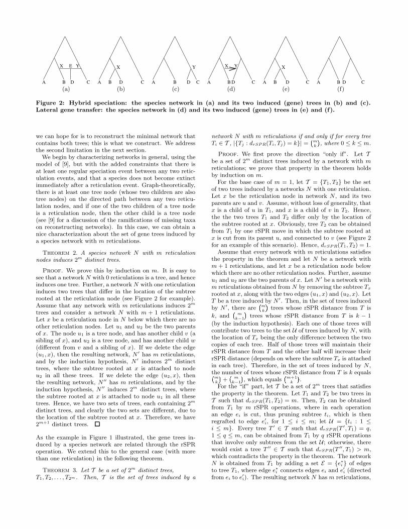
It is clear that trees are inappropriate graphical modelsof species evolution when reticulation occurs, though stillappropriate for gene evolution: in hybrid speciation, twolineages recombine to create a new species, as symbolizedin Figure 2(a), but genes evolve down trees contained inthe network as shown in Figures 2(b) and (c). In lateral(i.e., horizontal) gene transfer, genetic material is trans-ferred from one lineage to another without resulting in theproduction of a new lineage, as symbolized in Figure 2(d).And, as in hybrid speciation, each site evolves down a treewithin the network; that is, some sites are inherited throughlateral transfer from another species, as in Figure 2(e), whileall others are inherited from the parent, as in Figure 2(f).
3.1 Maddison’s approach to phylogeny recon-struction
In 1997, Wayne Maddison [10] made an important obser-vation which directly suggests a technique for reconstructingphylogenetic networks, via a “separate analysis” approach,which we now describe. Maddison observed that when thereis one reticulation in the network, there are two trees withinthe network, and every gene evolves down one of these twogene trees. Furthermore, the two trees are related to eachother by a single rSPR move, and given the two trees, itis straightforward to construct the network that containedboth trees. Maddison also suggested that when the networkcontains m reticulations, then any two trees contained in
the network would be related to each other by a sequenceof at most m rSPR moves (though the specific technique forproducing the network from two of its constituent trees wasnot provided). Maddison’s observations imply the followingmethod for constructing phylogenetic networks:
• Step 1: For each gene dataset, infer a gene tree.
• Step 2: If the two trees are identical, return that tree.Else, find the minimum network that contains bothtrees.
While Maddison showed how to perform Step 2 when theminimum network contains a single reticulation, he left openhow to do Step 2 when the network contains more thanone reticulation. However, finding such a network requirescomputing the rSPR distance between the two binary genetrees. This is a problem of unknown computational com-plexity, which is a computational limitation of Maddison’sapproach.
The other limitation is potentially more serious: if thegene trees have errors in them, then the minimal networkthat contains the gene trees may be incorrect. Therefore,Maddison’s method needs to be modified to work with errorsin the estimated gene trees.
In this paper we address both problems. In Section 4 weshow how to reconstruct a gt-network with any number ofreticulations from accurate gene trees (under an additionalassumption about the network). In Sections 5 and 6 we showhow to reconstruct a network with a single reticulation fromgene tree estimates that need not be accurate. In our futurework, we will investigate how to combine these approaches.
4. RECONSTRUCTING GT-NETWORKSWHEN GENE TREE ESTIMATES AREACCURATE
There are two main limitations to Maddison’s approach:(1) the construction of a network from two gene trees is onlydescribed explicitly when the network contains exactly onereticulation; (2) obtaining accurate binary trees in practicemay not be possible in most cases. In this section we addressthe first limitation by showing how to accurately constructa gt-network, with any number of reticulations, from two ofits constituent gene trees. However, since any two gene treesmay not involve both parents in each reticulation, the best
A B
X E
D C
Y
A B D C
X
A B CD
Y
A B CD
X Y
A CB D
X
A CB D
(a) (b) (c) (d) (e) (f)
Figure 2: Hybrid speciation: the species network in (a) and its two induced (gene) trees in (b) and (c).Lateral gene transfer: the species network in (d) and its two induced (gene) trees in (e) and (f).
we can hope for is to reconstruct the minimal network thatcontains both trees; this is what we construct. We addressthe second limitation in the next section.
We begin by characterizing networks in general, using themodel of [9], but with the added constraints that there isat least one regular speciation event between any two retic-ulation events, and that a species does not become extinctimmediately after a reticulation event. Graph-theoretically,there is at least one tree node (whose two children are alsotree nodes) on the directed path between any two reticu-lation nodes, and if one of the two children of a tree nodeis a reticulation node, then the other child is a tree node(see [9] for a discussion of the ramifications of missing taxaon reconstructing networks). In this case, we can obtain anice characterization about the set of gene trees induced bya species network with m reticulations.
Theorem 2. A species network N with m reticulationnodes induces 2m distinct trees.
Proof. We prove this by induction on m. It is easy tosee that a network N with 0 reticulations is a tree, and henceinduces one tree. Further, a network N with one reticulationinduces two trees that differ in the location of the subtreerooted at the reticulation node (see Figure 2 for example).Assume that any network with m reticulations induces 2m
trees and consider a network N with m + 1 reticulations.Let x be a reticulation node in N below which there are noother reticulation nodes. Let u1 and u2 be the two parentsof x. The node u1 is a tree node, and has another child v (asibling of x), and u2 is a tree node, and has another child w(different from v and a sibling of x). If we delete the edge(u1, x), then the resulting network, N ′ has m reticulations,and by the induction hypothesis, N ′ induces 2m distincttrees, where the subtree rooted at x is attached to nodeu2 in all these trees. If we delete the edge (u2, x), thenthe resulting network, N ′′ has m reticulations, and by theinduction hypothesis, N ′′ induces 2m distinct trees, wherethe subtree rooted at x is attached to node u1 in all thesetrees. Hence, we have two sets of trees, each containing 2m
distinct trees, and clearly the two sets are different, due tothe location of the subtree rooted at x. Therefore, we have2m+1 distinct trees.
As the example in Figure 1 illustrated, the gene trees in-duced by a species network are related through the rSPRoperation. We extend this to the general case (with morethan one reticulation) in the following theorem.
Theorem 3. Let T be a set of 2m distinct trees,T1, T2, . . . , T2m . Then, T is the set of trees induced by a
network N with m reticulations if and only if for every treeTi ∈ T , |{Tj : drSPR(Ti, Tj) = k}| =
�m
k � , where 0 ≤ k ≤ m.
Proof. We first prove the direction “only if”. Let Tbe a set of 2m distinct trees induced by a network with mreticulations; we prove that property in the theorem holdsby induction on m.
For the base case of m = 1, let T = {T1, T2} be the setof two trees induced by a networks N with one reticulation.Let x be the reticulation node in network N , and its twoparents are u and v. Assume, without loss of generality, thatx is a child of u in T1, and x is a child of v in T2. Hence,the the two trees T1 and T2 differ only by the location ofthe subtree rooted at x. Obviously, tree T2 can be obtainedfrom T1 by one rSPR move in which the subtree rooted atx is cut from its parent u, and connected to v (see Figure 2for an example of this scenario). Hence, drSPR(T1, T2) = 1.
Assume that every network with m reticulations satisfiesthe property in the theorem and let N be a network withm + 1 reticulations, and let x be a reticulation node belowwhich there are no other reticulation nodes. Further, assumeu1 and u2 are the two parents of x. Let N ′ be a network withm reticulations obtained from N by removing the subtree Tx
rooted at x, along with the two edges (u1, x) and (u2, x). LetT be a tree induced by N ′. Then, in the set of trees inducedby N ′, there are
�m
k � trees whose rSPR distance from T is
k, and�
m
k−1 � trees whose rSPR distance from T is k − 1
(by the induction hypothesis). Each one of those trees willcontribute two trees to the set U of trees induced by N , withthe location of Tx being the only difference between the twocopies of each tree. Half of those trees will maintain theirrSPR distance from T and the other half will increase theirrSPR distance (depends on where the subtree Tx is attachedin each tree). Therefore, in the set of trees induced by N ,the number of trees whose rSPR distance from T is k equals�
m
k � +�
m
k−1 � , which equals�m+1
k � .For the “if” part, let T be a set of 2m trees that satisfies
the property in the theorem. Let T1 and T2 be two trees inT such that drSPR(T1, T2) = m. Then, T2 can be obtainedfrom T1 by m rSPR operations, where in each operationan edge ei is cut, thus pruning subtree ti, which is thenregrafted to edge e′i, for 1 ≤ i ≤ m; let U = {ti : 1 ≤i ≤ m}. Every tree T ′ ∈ T such that drSPR(T ′, T1) = q,1 ≤ q ≤ m, can be obtained from T1 by q rSPR operationsthat involve only subtrees from the set U ; otherwise, therewould exist a tree T ′′ ∈ T such that drSPR(T ′′, T1) > m,which contradicts the property in the theorem. The networkN is obtained from T1 by adding a set E = {e∗i } of edgesto tree T1, where edge e∗i connects edges ei and e′i (directedfrom ei to e′i). The resulting network N has m reticulations,
u1, u2, . . . , um, and it induces the 2m trees in T .
4.1 Efficient reconstruction of gt-networks fromgene trees
Theorem 3 implies that given the “full” set of trees in-duced by a gt-network, we can reconstruct the network viaa series of rSPR distance computations among the trees.However, given a pair of trees induced by a gt-network, wecan only reconstruct a minimal (in terms of the number ofreticulation nodes) gt-network that induces these two trees.In what follows, we show how to efficiently reconstruct sucha minimal network from a pair of trees. Hereafter, we usen to denote the number of leaves in the trees as well asnetworks.
The intuition behind our algorithm is as follows. Giventwo trees T1 and T2, induced by a gt-network N , we first“mark” the edges of each tree that are incompatible withthe other tree (symbolized by U(T1, T2) and U(T2, T1) inthe proofs). If the two trees are m rSPR moves apart, themarked edges in tree T1 would form m node-disjoint paths inT1, and similarly for tree T2. While necessary, this conditionis not sufficient; an extra step is needed, in which, for eachmaximal path p1 of marked edges in T1, there must exist aunique maximal path p2 of marked edges in T2, where theendpoints of the two paths correspond to one rSPR move.
Lemma 1. Let T1 and T2 be two trees induced by a gt-network N . Further, assume that gall Qw
x in N was bro-ken in the two different ways to obtain T1 and T2. Then,RP Q(T1) ⊆ U(T1, T2), and RP Q(T2) ⊆ U(T2, T1).
Proof. Let RP Q be formed of the two paths p1 and p2
whose tail is w. Further, assume p1 is the path attached toedge e1 and p2 is the path attached to e2, where RE(Q) ={e1, e2}. Let X be the subtree rooted at node x, T1 beobtained by removing edge e1 from Q, and T2 be obtainedby removing edge e2 from Q. Then, in T1, the leaves ofX are under the edges of p2 but not under the edges ofp1, whereas in T2, the leaves of X are under the edges of p1
but not under the edges of p2. Hence, the edges on RP Q(T1)are incompatible with the edges of RP Q(T2), and vice versa.Therefore, we have RP Q(T1) ⊆ U(T1, T2) and RP Q(T2) ⊆U(T2, T1).
Lemma 2. Let T1 and T2 be two trees induced by a gt-network N . Further, assume that gall Q in N was brokenin exactly the same way to obtain both T1 and T2. Then,RP Q(T1) ∩ U(T1, T2) = ∅, and RP Q(T2) ∩ U(T2, T1) = ∅.
Proof. Since the gall Q is broken in exactly the sameway to obtain the two trees T1 and T2, it follows that theedges on RP Q(T1) induce the same bipartitions as thoseinduced by the edges of RP Q(T2). Hence, the edges ofRP Q(T1) and RP Q(T2) are mutually compatible. Further,the edges of RP Q(T1) are compatible with E(T2)\RP Q(T2);otherwise, the network N would not be a gt-network (therewould be two “overlapping” galls). Similarly, the edges ofRP Q(T2) are compatible with E(T1) \RP Q(T1). Therefore,it follows that RP Q(T1) ∩ U(T1, T2) = ∅ and RP Q(T2) ∩U(T2, T1) = ∅.
Let T be a tree induced by a gt-network N . We denote byNG(T ) the set of all edges e that are not on any gall inN . Formally, NG(T ) = {e ∈ E(T ) : for all galls Q in N ,e /∈ RP Q(T )}.
Lemma 3. Let T1 and T2 be two trees induced by a gt-network N . Then, NG(T1) ∩ U(T1, T2) = ∅, and NG(T2) ∩U(T2, T1) = ∅.
Proof. Assume e = (u, v) is an edge in NG(T1)∩U(T1, T2).Let A be the subtree of T1 rooted at v. Since e ∈ U(T1, T2),then, for some edge e′ = (u′, v′) in T2, L(A) ∩ L(B) 6= ∅,where B is the subtree of T2 rooted at v′. Let X = L(A) \(L(A) ∩ L(B)). Then, in tree T1, X is under edge e, andin tree T2, X is not under edge e′. Hence, edges e and e′
are members of E(Q) for some gall Q; a contradiction thate ∈ NG(T1). Therefore, NG(T1) ∩ U(T1, T2) = ∅; similarly,we prove that NG(T2) ∩ U(T2, T1) = ∅.
Theorem 4. Let N be a gt-network with q galls{Q1, Q2, . . . , Qq}, and T1 and T2 be two trees induced by N .Further, assume that exactly m of the q galls were brokenin the two possible ways to obtain the two trees T1 and T2,and the other q − m galls were each broken in a single way.Then, U(T1, T2) forms m node-disjoint undirected paths inT1, and U(T2, T1) forms m node-disjoint undirected paths inT2.
The proof follows immediately from Lemma 1, Lemma 2,and Lemma 3, and is omitted. Stated differently, Theo-rem 4 implies that if T1 and T2 are two trees induced bya gt-network N such that drSPR(T1, T2) = m, then each ofthe two sets U(T1, T2) and U(T2, T1) forms m node-disjointundirected paths in T1 and T2, respectively.
Let T1 and T2 be two trees induces by a gt-network N ,such that U(T1, T2) forms a set of node-disjoint undirectedpaths in T1, and U(T2, T1) forms a set of node-disjoint undi-rected paths in T2. Let p1 be one such path in U(T1, T2),and p2 be one such path in U(T2, T1). Further, assumeEND(p1) = (U1, V1) and END(p2) = (U2, V2). We saythat p1 yields p2 in one rSPR move (via subtree X),denoted p1 |=X p2, if there exists a nonempty subtree Xsuch that (1) X is a subtree of either U1 or V1, (2) X is asubtree of either U2 or V2, and (3) p1 ∩ U(T ′
1, T′2) = ∅ and
p2 ∩ U(T ′2, T
′1) = ∅, where T ′
1 = T1 \ X and T ′2 = T2 \ X.
Theorem 5. Let T1 and T2 be two trees induced by agt-network N . Further, assume that U(T1, T2) forms a setP1 of m node-disjoint undirected paths p1
1, p12, . . . , p
1m in T1,
and U(T2, T1) forms a set P2 of m node-disjoint undirectedpaths p2
1, p22, . . . , p
2m in T2. Then, drSPR(T1, T2) = m if
there is an injective function f : P1 → P2 and m subtreesX1, X2, . . . , Xm such that f(p1
i ) = p2j iff p1
i |=Xi p2j , where
1 ≤ i, j ≤ m.
Proof. Let P1 and P2 be the two sets of paths in thelemma, and let f be the injective function. Let p1
i ∈ P1 andp2
j ∈ P2 be two paths such that f(p1i ) = f(p2
j ). Assume Xi
is the subtree such that p1i |=Xi p2
j . Then, Xi is the subtreewhose pruning from T1 and regrafting it to another edge (toobtain tree T2) yielded paths p1
i and p2j in the two trees,
respectively. Since there are m such pairs of paths, thereare m such subtrees Xi whose pruning and regrafting in T1
would yield a tree T such that U(T1, T2) = ∅, which impliesT = T1. Hence, drSPR(T1, T2) = m.
Theorem 6. Let T1 and T2 be two binary trees induced bya gt-network N . We can decide whether drSPR(T1, T2) = min O(mn) time.
Proof. Preprocess the trees so that (1) For every twoleaves si and sj in either tree, the least common ancestor(LCA) of these two leaves can be found in constant time.This can be achieved in O(n) time using the techniques from[3, 7], and (2) For any internal nodes, i, the number β(i) ofleaves below i can be found in constant time. Further, ifSi is the set of leaves under i, then LCA(Si) can be foundin constant time. This can be achieved in O(n) time usingthe techniques from [3]. After this preprocessing, comput-ing U(T1, T2) and U(T2, T1) takes O(n) time (O(1) time foreach edge, and there are O(n) edges). This can be done byobserving that an edge e = (u, v) is in U(T1, T2) if and onlyif β(i) 6= β(LCA(Si)) (i is the number assigned to node v).It takes O(n) time to check if U(T1, T2) forms a simple path.Further, it takes O(n) time to check if the conditions of The-orem 4 and Theorem 5 hold (we can find f(p1
i ), if it exists,in O(1) time, by using the “highest” node of path p1
i andfinding its counterpart in T2; to find that subtree Xi suchthat p1
i |=X p2j , we need to compute the four pairwise inter-
sections of a set in END(p1i ) and a set in END(p2
j ), eachof which takes O(n) time, using bit vector representation ofsets). Hence, we can decide whether drSPR(T1, T2) = m inO(mn) time.
Now, it is straightforward to construct a gt-network N withm galls in O(mn) time, given two induced trees T1 and T2
such that drSPR(T1, T2) = m.
Theorem 7. Let T1 and T2 be two binary trees such thatdrSPR(T1, T2) = m. We can decide whether T1 and T2 areinduced by a gt-network N with m reticulation events, andif so construct such N , in O(mn) time.
Proof. By Theorem 6, we can find the m subtrees{X1, . . . , Xm}, such that p1
i |=Xi p2i , for 1 ≤ i ≤ m, where
p1i is a path in U(T1, T2), p2
i is a path in U(T2, T1), andf(p1
i ) = p2i (f is the injective function in the definition of
|=X). All this can be done in O(mn) time. We form the gt-network N from T1 as follows. For each path p1
i in U(T1, T2)and its corresponding subtree Xi, Xi will be attached to oneend of p1
i . We add another edge from the other end of p1i to
the root of Xi, thus creating a network N with m galls. Sincethe paths are node-disjoint, N will be a gt-network.
5. RECONSTRUCTING GT-NETWORKSWHEN GENE TREE ESTIMATES AREINACCURATE
The main limiting factor in Maddison’s approach is thatmethods, even if statistically consistent, can fail to recoverthe true tree. Even on quite long sequences, some topo-logical error is often present. This topological error can betolerated in a phylogenetic analysis, but it makes the infer-ence of phylogenetic networks from constituent gene treesdifficult. To overcome these limits, we propose a methodthat allows for error in the estimates of the individual genetrees; consequently, our method performs much better inpractice (as our simulation studies show).
Before we describe the method, we provide some insightinto its design. When methods such as maximum parsi-mony or maximum likelihood are used to infer trees, typi-cally a number of trees is returned, rather than a single besttree. For example, in maximum parsimony searches, es-pecially with larger datasets, there are often many equally
good trees (all having the same best score), and all canbe returned (along with suboptimal trees, if desired). Inmaximum likelihood, although the best-scoring tree may beunique, the difference in quality between that tree and thenext best tree(s) can be statistically insignificant, and soagain, a number of trees can be returned [14]. A commonoutput of a phylogenetic analysis is the strict consensus ofthese trees (that is, the most resolved common contractionof all the best trees found).
The interesting, and highly relevant, point here is the fol-lowing observation, supported by both empirical studies onreal datasets and simulations: the strict consensus tree willoften be a contraction of the true tree. Thus, even when ev-ery tree in the set of best trees is a little bit wrong, the strictconsensus tree (which contains only those edges common toall the best trees) is likely to be a contraction of the truetree. This observation suggests the following approach toinferring phylogenetic networks.• Proposed Approach
• Step 1: For each gene dataset, use a method (suchas maximum parsimony or maximum likelihood) ofchoice, to construct a set of “best” trees, thus pro-ducing sets T1 and T2.
• Step 2: Compute the strict consensus tree ti for Ti,for i = 1, 2.
• Step 3: Find trees T1 and T2 refining t1 and t2 suchthat Ti refines ti for each i = 1, 2, and T1 and T2 areinduced trees within a gt-network with p reticulations,for some minimum p.
When p = 0, the two consensus trees are compatible, and wewould return the compatibility tree; see Section 2.1. We nowshow how to handle the third step in this method when p = 1(solving this for general p is currently an open problem). Inthis case, Step 3 involves solving the following problem.• Combining consensus trees into a network(the ConsTree-Network Problem)
• Input: Two trees, t1 and t2, on the same set of leaves(not assumed to be binary)
• Output: A network N inducing trees T1 and T2, suchthat N contains one reticulation, and Ti refines ti, fori = 1, 2, if it exists; else fail.
We now provide a linear-time algorithm for this problem.There are two cases to consider: when the two consensustrees are compatible, and when the two trees are incompat-ible.
5.1 Compatible consensus treesIn most cases, if the consensus trees share a common re-
finement, we might believe the evolution to be tree-like (inwhich case we should combine the datasets, and analyze atree directly). However, suppose we have reason to believethat a dataset has undergone reticulation, so that a treeis not an appropriate representation of the true tree. Inthis case, we can still seek reticulate evolutionary scenarioscompatible with our observations. We begin with a simplelemma.
Observation 1. Let t be a binary tree that refines anunresolved tree T , and let p be a path in tree t. Then, whenrestricted to the edges of T , p forms a path in T as well.
Lemma 4. Let t be an unresolved tree. Then, there ex-ist two binary trees T1 and T2 that refine t and such thatdrSPR(T1, T2) = 1.
Proof. Let x be a node with outdegree 3, and let v1, v2,and v3 be the three children of node x. We obtain T1 from tby removing the edges (x, v1) and (x, v2), adding a new nodeu with an edge (x, u), and then making v1 and v2 childrenof u. The tree T2 can be obtained from t by removing theedges (x, v2) and (x, v3), adding a new node u with an edge(x, u), and then making v2 and v3 children of u. The rest ofthe nodes of T1 and T2 are resolved identically in both trees.It is obvious that T2 can be obtained from T1 by pruning v2
from its parent and attaching it to edge (x, v3) in T1, andhence drSPR(T1, T2) = 1.
Lemma 4 can be generalized to the case where t1 and t2 aretwo unresolved, yet compatible trees, as follows.
Lemma 5. Let t1 and t2 be two compatible unresolved trees.Then, there exist two binary trees T1 and T2 that refine t1and t2 respectively, and drSPR(T1, T2) = 1 if and only if t1and t2 have a common refinement t that is not fully resolved.Furthermore, we can determine if these two trees exist, andconstruct them, in O(n) time.
Proof. The proof of the “if” part follows from Lemma 4.We prove the “only if” part. Let T1 and T2 be two binarytrees that refine two unresolved (compatible) trees t1 and t2,such that drSPR(T1, T2) = 1. Since t1 and t2 are compatible,then they share a common refinement, t. The two binarytrees T1 and T2 also refine t. Since T1 and T2 are differentbinary trees and refine the same tree t, it follows that t isnot fully resolved.
5.2 Incompatible consensus treesWe now address the last remaining case, where the consen-
sus trees are incompatible. We begin with a simple lemma.
Lemma 6. Let T1 and T2 be two binary trees that refinetwo unresolved trees t1 and t2. Then, U(t1, t2) ⊆ U(T1, T2).
Proof. Let e ∈ U(t1, t2). Then, e ∈ E(t1), and conse-quently e ∈ E(T1). Further, e is incompatible with t2, andhence is incompatible with T2. It follows that e ∈ U(T1, T2).Therefore, U(t1, t2) ⊆ U(T1, T2).
Lemma 7. Let t1 and t2 be two unresolved incompatibletrees. If there exist two binary trees T1 and T2 that refine t1and t2, respectively, and such that drSPR(T1, T2) = 1, thenU(t1, t2) and U(t2, t1) are both simple paths in t1 and t2,respectively.
Proof. Assume U(t1, t2) is not a simple path in t1. Then,by Theorem 4, it follows that U(T1, T2) is not a simple pathin T1, and hence drSPR(T1, T2) 6= 1; a contradiction. There-fore, U(t1, t2) forms a simple path in t1. Similarly, we es-tablish that U(t2, t1) forms a simple path in t2.
Lemma 8. Let t1 and t2 be two incompatible unresolvedtrees, such that U(t1, t2) forms a path p1 in t1, and U(t2, t1)forms a path p2 in t2. Further, let END(p1) = (A1, B1) andEND(p2) = (A2, B2). Let Xi, 1 ≤ i ≤ 4, be the followingfour sets: X1 = (A1 − A2) ∩ (B2 − B1), X2 = (A1 − B2) ∩(A2 − B1), X3 = (B1 − A2) ∩ (B2 − A1), and X4 = (B1 −
B2) ∩ (A2 − A1). Then, there exist two binary trees T1 andT2 that refine t1 and t2, respectively, and drSPR(T1, T2) = 1,if and only if there exists an i, 1 ≤ i ≤ 4, such that (C1)t1|S\Xi
and t2|S\Xiare compatible, (C2) t1|Xi
and t2|Xi
are compatible, and (C3) t1|S\Xicontains all the edges in
U(t1, t2), and t2|S\Xicontains all the edges in U(t2, t1).
Proof. Assume that Xi, for some 1 ≤ i ≤ 4, satis-fies both conditions C1 and C2. Then, resolve t1|S\Xi
andt2|S\Xi
identically, resolve t1|Xiand t2|Xi
identically, andfinally attach the resolved subtrees t1|Xi
and t2|Xiin their
corresponding subtrees. The result is obviously two binarytrees T1 and T2 that differ only in the location of the subtreeleaf-labeled by Xi; i.e., drSPR(T1, T2) = 1. Let T1 and T2
be two binary trees that resolve the two incompatible un-resolved trees t1 and t2, such that drSPR(T1, T2) = 1. ByLemma 6, p1 ⊆ U(T1, T2) and p2 ⊆ U(T2, T1). By Theo-rem 5, T2 can be obtained from T1 by pruning a subtreet′ from one side of the path U(T1, T2) and regrafting it onthe other side of the path. It follows that t1|S\L(t′) andt2|S\L(t′) are compatible, and also that t1|L(t′) and t2|L(t′)
are compatible (since they refine the same tree t′). It isstraightforward to verify that L(t′) is equal to Xi, for some1 ≤ i ≤ 4.
We now state the major theorem of this section.
Theorem 8. We can solve the ConsTree-Network Prob-lem in O(n) time. That is, given two unresolved trees t1 andt2, in O(n) time we can find two binary trees T1 and T2 thatrefine t1 and t2, respectively, such that drSPR(T1, T2) = 1,when such a pair of trees exist. Further, once we have T1 andT2, we can compute a phylogenetic network with exactly onereticulation event inducing these trees in O(n) additionaltime.
Proof. We preprocess the trees so that: (1) For everytwo leaves si and sj in either tree, the least common ancestor(LCA) of these two leaves can be found in constant time.This can be achieved in O(n) time using the techniques from[3, 7], and (2) For any internal node, i, the number β(i) ofleaves below i can be found in constant time. Further, ifSi is the set of leaves under i, then LCA(Si) can be foundin constant time. This can be achieved in O(n) time usingthe techniques from [3]. After this preprocessing, computingU(t1, t2) takes O(n) time (O(1) time for each edge, and thereare O(n) edges). It takes O(n) time to check if U(t1, t2)forms a simple path. By Lemmas 7 and 8, we first checkwhether U(t1, t2) and U(t2, t1) form simple paths. Then, wecheck whether conditions C1 and C2 of Lemma 8 hold; if so,then we can obtain two binary trees T1 and T2 that resolve t1and t2, such that drSPR(T1, T2) = 1. Having preprocessedthe trees, testing the conditions of these two lemmas canbe achieved in O(n) time. Using bit vectors to representthe sets of taxa, we can preprocess the trees in O(n) timesuch that we store at each node the set of taxa under it;hence, it takes O(n) time to compute the sets Xi, 1 ≤ i ≤ 4.We construct N from T1 and T2 using in O(n) time usingTheorem 7. Hence, the algorithm takes O(n) time.
6. SPNET: OUR TECHNIQUE FOR INFER-RING GT-NETWORKS
SpNet, for Species Network, is a method we have de-signed for inferring networks (or trees, depending on the
data) under realistic conditions. We base SpNet on theapproach we outlined in the previous section, but we specif-ically use maximum likelihood for tree reconstruction, andwe compute the strict consensus of the best two trees foreach dataset. In order to facilitate a comparison to othermethods, such as NeighborNet, we do not allow SpNet toreturn “fail”, and so we apply Neighbor Joining (NJ) to allinputs on which we would otherwise return “fail.”• SpNet
• Step 1: We find the best two trees on each datasetunder maximum likelihood,
• Step 2: For each dataset, we compute the strict con-sensus of the two trees, thus producing the trees t1 andt2, and
• Step 3: If t1 and t2 are compatible, we combinedatasets and analyze the combined (i.e., concatenated)dataset using NJ, thus returning a tree. Else, we applyour algorithm for ConsTree-Network to t1 and t2. Ifwe can, we return a network N with one reticulation(if trees T1 and T2 exist refining t1 and t2, respectively,contained within the network N); if no such networkexists, we apply NJ to the concatenated dataset, andreturn a tree. (Alternatively, we could simply return“fail”.)
6.1 Experimental resultsWe have done extensive studies evaluating the perfor-
mance of the SpNet method in simulation, and comparedthe method to NeighborNet, NJ, and Maddison’s method.Not surprisingly, the method outperforms Maddison’s methodsince it is designed to allow for error in the data. Interest-ingly, it also outperforms NJ when the data are generatedon a network with a reticulation (it has essentially identicalperformance to NJ when the data are generated by a tree,which is not surprising). The comparison between SpNet
and NeighborNet is more interesting, and is the focus of ourbrief discussion here.
We focus here on the results of our experiments on 20-taxon trees and networks with one reticulation. We sim-ulated evolution down these trees and networks (using thetools in [11]) under the GTR model with gamma distributedrates across sites, and invariant sites (using the settings of[18]); reticulations in the networks modelled hybrid speci-ation. We produced two sequence datasets for each net-work, one for each of the gene trees contained within thenetwork. The concatenated sequences were given to bothNJ and NeighborNet (since those two methods are based ona combined analysis approach), but the separate gene se-quences were given to SpNet (since this method is based ona separate analysis approach). Furthermore, concatenatedsequences are required by both NJ and NeighborNet becausethey operate on distance matrices produced from all of thedata used in an analysis.
We measured the topological accuracy of the inferred phy-logenies (both trees and networks) with respect to the modelnetwork as follows. We define C(N)–the bipartitions of anetwork N–as the set of all bipartitions induced by the treescontained inside N ; in other words,
C(N) = �T∈T (N)
C(T )
where T (N) is the set of all trees induced by network N .
Given two networks, Nm (the model network) and Ni (theinferred network), we define the false positives, which isthe number of incorrectly inferred bipartitions, as |C(Ni)−C(Nm)|, and the false negatives, which is the number ofmissing bipartitions, as |C(Nm)−C(Ni)|. To obtain the falsepositive rate (FP) and false negative rate (FN), we normal-ize both the false positives and false negatives by the numberof bipartitions in the model network (|C(Nm)|). Hence, theFN rate of any method is at most 100%, whereas the FNrate may be larger than 100%.
False negative and false positive rates below 10% are good,with rates below 5% very good, in evaluating tree recon-struction methods.
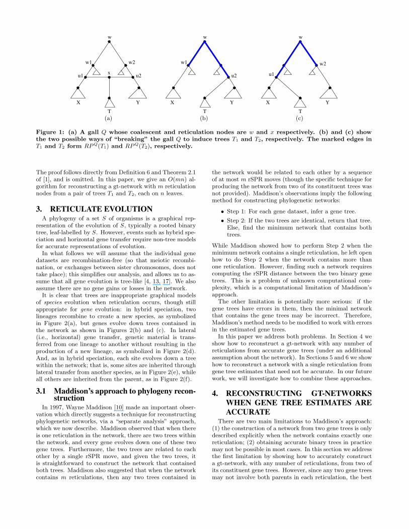
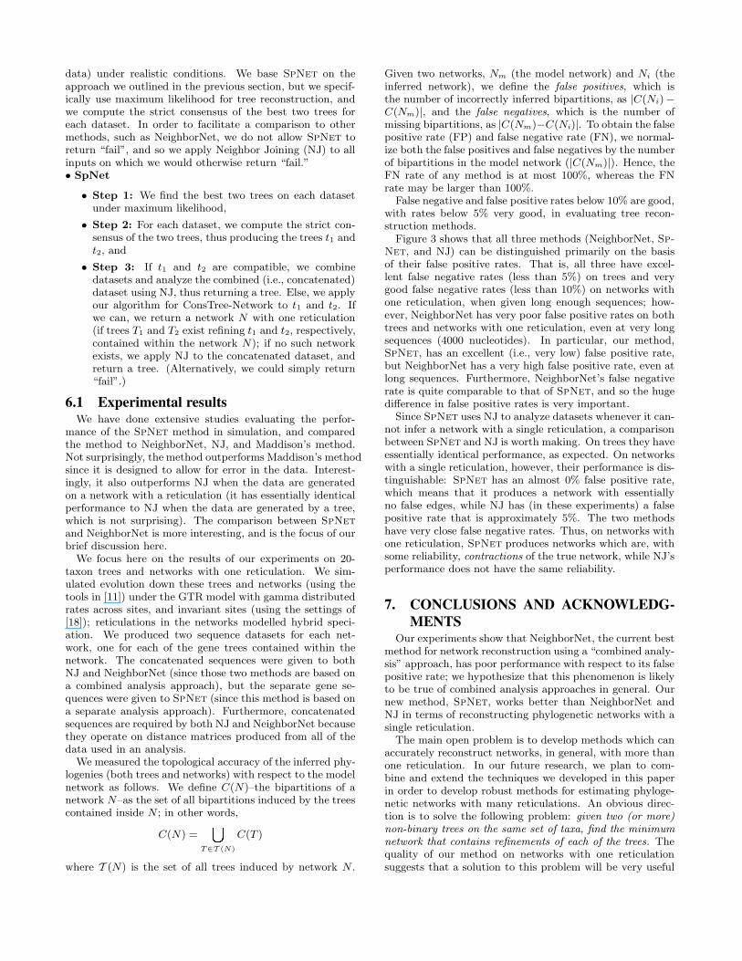
Figure 3 shows that all three methods (NeighborNet, Sp-
Net, and NJ) can be distinguished primarily on the basisof their false positive rates. That is, all three have excel-lent false negative rates (less than 5%) on trees and verygood false negative rates (less than 10%) on networks withone reticulation, when given long enough sequences; how-ever, NeighborNet has very poor false positive rates on bothtrees and networks with one reticulation, even at very longsequences (4000 nucleotides). In particular, our method,SpNet, has an excellent (i.e., very low) false positive rate,but NeighborNet has a very high false positive rate, even atlong sequences. Furthermore, NeighborNet’s false negativerate is quite comparable to that of SpNet, and so the hugedifference in false positive rates is very important.
Since SpNet uses NJ to analyze datasets whenever it can-not infer a network with a single reticulation, a comparisonbetween SpNet and NJ is worth making. On trees they haveessentially identical performance, as expected. On networkswith a single reticulation, however, their performance is dis-tinguishable: SpNet has an almost 0% false positive rate,which means that it produces a network with essentiallyno false edges, while NJ has (in these experiments) a falsepositive rate that is approximately 5%. The two methodshave very close false negative rates. Thus, on networks withone reticulation, SpNet produces networks which are, withsome reliability, contractions of the true network, while NJ’sperformance does not have the same reliability.
7. CONCLUSIONS AND ACKNOWLEDG-MENTS
Our experiments show that NeighborNet, the current bestmethod for network reconstruction using a “combined analy-sis” approach, has poor performance with respect to its falsepositive rate; we hypothesize that this phenomenon is likelyto be true of combined analysis approaches in general. Ournew method, SpNet, works better than NeighborNet andNJ in terms of reconstructing phylogenetic networks with asingle reticulation.
The main open problem is to develop methods which canaccurately reconstruct networks, in general, with more thanone reticulation. In our future research, we plan to com-bine and extend the techniques we developed in this paperin order to develop robust methods for estimating phyloge-netic networks with many reticulations. An obvious direc-tion is to solve the following problem: given two (or more)non-binary trees on the same set of taxa, find the minimumnetwork that contains refinements of each of the trees. Thequality of our method on networks with one reticulationsuggests that a solution to this problem will be very useful
1000 2000 3000 40000
0.5
1
1.5
2
Sequence Length
Err
or R
ate
FN(NNet)FN(SpNet)FP(NNet)FP(SpNet)FN(NJ)FP(NJ)
1000 2000 3000 40000
0.5
1
1.5
2
Sequence Length
Err
or R
ate
FN(NNet)FN(SpNet)FP(NNet)FP(SpNet)FN(NJ)FP(NJ)
1000 2000 3000 40000
0.1
0.2
0.3
0.4
0.5
Sequence Length
Err
or R
ate
FN(NNet)FN(SpNet)FP(SpNet)FN(NJ)FP(NJ)
Figure 3: FN and FP error rates of NeighborNet (NNet) and SpNet on 20-taxon networks, with 0.1 scalingfactor, with tree model phylogeny (left), and 1-hybrid network (middle). The rightmost graph shows theresults without the FP rate of NNet.
for phylogenetic network reconstruction, and should havebetter accuracy (with respect to false positives) than exist-ing approaches. However, the problem remains of unknowncomputational complexity, even for gt-networks.
This work is supported by National Science Foundationunder grants DEB 01-20709 (Linder & Warnow), EIA 01-21651 (Warnow), EIA 01-13654 (Warnow), EIA 01-21680(Linder & Warnow), EF 01-31453 (Linder & Warnow), bythe David and Lucile Packard Foundation (Warnow), by theInstitute for Cellular and Molecular Biology at UT-Austin(Warnow), by the Program in Evolutionary Dynamics atHarvard University (Warnow), and by the Radcliffe Institutefor Advanced Study (Warnow).
8. REFERENCES[1] B. Allen and M. Steel. Subtree transfer operations and
their induced metrics on evolutionary trees. Annals ofCombinatorics, 5:1–13, 2001.
[2] D. Bryant and V. Moulton. NeighborNet: Anagglomerative method for the construction of planarphylogenetic networks. In R. Guigo and D. Gusfield,editors, Proc. 2nd Workshop Algorithms inBioinformatics (WABI’02), volume 2452 of LectureNotes in Computer Science, pages 375–391. SpringerVerlag, 2002.
[3] W.H.E. Day. Optimal algorithms for comparing treeswith labeled leaves. Journal of Classification, 2:7–28,1985.
[4] S.B. Gabriel, S.F. Schaffner, H. Nguyen, J.M. Moore,J. Roy, B. Blumenstiel, J. Higgins, M. DeFelice,A. Lochner, M. Faggart, S.N. Liu-Cordero, C. Rotimi,A. Adeyemo, R. Cooper, R. Ward, E.S. Lander, M.J.Daly, and D. Altshuler. The structure of haplotypeblocks in the human genome. Science,296(5576):2225–2229, 2002.
[5] D. Gusfield. Efficient algorithms for inferringevolutionary trees. Networks, 21:19–28, 1991.
[6] D. Gusfield, S. Eddhu, and C. Langley. Efficientreconstruction of phylogenetic networks withconstrained recombination. In Proceedings ofComputational Systems Bioinformatics (CSB 03),2003.
[7] D. Harel and R.E. Tarjan. Fast algorithms for findingnearest common ancestors. SIAM Journal onComputing, 13(2):338–355, 1984.
[8] J.G. Lawrence and H. Ochman. Reconciling the manyfaces of lateral gene transfer. Trends in Microbiology,10:1–4, 2002.
[9] C.R. Linder, B.M.E. Moret, L. Nakhleh, A. Padolina,J. Sun, A. Tholse, R. Timme, and T. Warnow.Phylogenetic networks: generation, comparison, andreconstruction. Technical Report TR-CS-2003-26,University of New Mexico, 2003.
[10] W.P. Maddison. Gene trees in species trees.Systematic Biology, 46(3):523–536, 1997.
[11] L. Nakhleh, J. Sun, T. Warnow, C.R. Linder, B.M.E.Moret, and A. Tholse. Towards the development ofcomputational tools for evaluating phylogeneticnetwork reconstruction method. In Proc. 8th PacificSymposium on Biocomputing (PSB 03), pages315–326, 2003.
[12] R. Page and M.A. Charleston. Trees within trees:Phylogeny and historical associations. Trends inEcology and Evolution, 13:356–359, 1998.
[13] D. Posada and C. Wiuf. Simulating haplotype blocksin the human genome. Bioinformatics, 19(2):289–290,2003.
[14] H. Shimodaira and M. Hasegawa. Multiplecomparisons of log-likelihoods with applications tophylogenetic inference. Molecular Biology andEvolution, 16:1114–1116, 1999.
[15] L. Wang, K. Zhang, and L. Zhang. Perfectphylogenetic networks with recombination. Journal ofComputational Biology, 8(1):69–78, 2001.
[16] T. Warnow. Tree compatibility and inferringevolutionary history. Journal of Algorithms,16:388–407, 1994.
[17] K. Zhang and L. Jin. HaploBlockFinder: haplotypeblock analyses. Bioinformatics, 19(10):1300–1301,2003.
[18] D. Zwickl and D. Hillis. Increased taxon samplinggreatly reduces phylogenetic error. Systematic Biology,51(4):588–598, 2002.


