Recovering Facial Shape and Albedo using aStatistical Model of Surface Normal Direction

William A.P. Smith and Edwin R. HancockDepartment of Computer Science, The University of York

{wsmith, erh}@cs.york.ac.uk

Abstract

This paper describes how facial shape can be modelledusing a statistical model that captures variations in sur-face normal direction. To construct this model we makeuse of the azimuthal equidistant projection to map surfacenormals from the unit sphere to points on a local tangentplane. The variations in surface normal direction are cap-tured using the covariance matrix for the projected pointpositions. This allows us to model variations in face shapeusing a standard point distribution model. We train themodel on fields of surface normals extracted from rangedata and show how to fit the model to intensity data us-ing constraints on the surface normal direction provided byLambert’s law. We demonstrate that this process yields ac-curate facial shape recovery and allows an estimate of thealbedo map to be made from single, real world face images.

1. IntroductionShape-from-shading provides an alluring yet somewhat

elusive route to recovering 3D surface shape from single2D intensity images [15]. Unfortunately, the method hasproved ineffective in recovering realistic 3D face shape be-cause of real world albedo variations and local convexity-concavity instability due to the bas-relief ambiguity. Thisis of course a well known effect which is responsible fora number of illusions, including Gregory’s famous invertedmask [6]. The main problem is that the nose becomes im-ploded and the cheeks exaggerated [2]. It is for this reasonthat methods such as photometric stereo [5] have provenmore effective.

One way of overcoming this problem with single viewshape-from-shading is to use domain specific constraints.Several authors [1, 2, 8, 9, 16] have shown that, at the ex-pense of generality, the accuracy of recovered shape in-formation can be greatly enhanced by restricting a shape-from-shading algorithm to a particular class of objects. Forinstance, both Prados and Faugeras [8] and Castelan andHancock [2] use the location of singular points to enforce

convexity on the recovered surface. Zhao and Chellappa[16], on the other hand, have introduced a geometric con-straint which exploited the approximate bilateral symmetryof faces. This ‘symmetric shape-from-shading’ was usedto correct for variation in illumination. They employedthe technique for recognition by synthesis. However, therecovered surfaces were of insufficient quality to synthe-sise novel viewpoints. Atick et al. [1] proposed a statisti-cal shape-from-shading framework based on a low dimen-sional parameterisation of facial surfaces. Principal com-ponents analysis (PCA) was used to derive a set of ‘eigen-heads’ which compactly captures 3D facial shape. Unfortu-nately, it is surface orientation and not depth which is con-veyed by image intensity. Therefore, fitting the model toan image equates to a computationally expensive parame-ter search which attempts to minimise the error between therendered surface and the observed intensity. This is sim-ilar to the approach adopted by Samaras and Metaxas [9]who incorporate reflectance constraints derived from shape-from-shading into a deformable model.

Previous work has shown that both images of faces[13] and facial surfaces [1] can be modelled in a low-dimensional space, derived by applying PCA to a trainingset of images or surfaces. Unfortunately, the construction ofa statistical model for the distribution of facial needle-mapsis not a straightforward task. The statistical representationof directional data has proved to be considerably more dif-ficult than that for Cartesian data [7]. Surface normals canbe viewed as residing on a unit sphere and may be specifiedin terms of the elevation and azimuth angles. This repre-sentation makes the computation of distance difficult. Forinstance, if we consider a short walk across one of the polesof the unit sphere, then although the distance traversed issmall, the change in azimuth angle is large. Hence, con-structing a statistical model that can capture the statisticaldistribution of directional data is not a straightforward task.

To overcome the problem, in this paper we draw onideas from cartography. Our starting point is the azimuthalequidistant or Postel projection [12]. This projection has theimportant property that it preserves the distances between

locations on the sphere. It is used in cartography for pathplanning tasks. Another useful property of this projection isthat straight lines on the projected plane through the centreof projection correspond to great circles on the sphere. Theprojection is constructed by selecting a reference point onthe sphere and constructing the tangent plane to the refer-ence point. Locations on the sphere are projected onto thetangent plane in a manner that preserves arc-length.

We exploit this property to generate a local representa-tion of the field of surface normals. We commence witha set of needle-maps, i.e. fields of surface normals whichin practice are obtained either from range images or shape-from-shading. We begin by computing the mean field ofsurface normals. The surface normals are represented us-ing elevation and azimuth angles on a unit sphere. At eachimage location the mean-surface normal defines a referencedirection. We use this reference direction to construct anazimuthal equidistant projection for the distribution of sur-face normals at each image location. The distribution ofpoints on the projection plane preserves the distances of thesurfaces normals on the unit sphere with respect to the meansurface normal. We then construct a deformable model overthe set of surface normals by applying the Cootes and Taylor[3] point distribution model to the co-ordinates that resultfrom transforming the surface normals from the unit sphereto the tangent plane under azimuthal equidistant projection.On the tangent projection plane, the points associated withthe surface normals are allowed to move in a manner whichis determined by the principal component directions of thecovariance matrix for the point-distribution. Once we havecomputed the allowed deformation movement on the tan-gent plane, we recover surface normal directions by usingthe inverse transformation onto the unit sphere.

We fit the model to 2D intensity images using ideasdrawn from shape-from-shading. When the surface re-flectance follows Lambert’s law, the surface normal is con-strained to fall on a cone whose axis is in the light sourcedirection and whose opening angle is the inverse cosine ofthe normalised image brightness. This method commencesfrom an initial configuration in which the surface normalsreside on the irradiance cone and point in the direction ofthe local image gradient. The statistical model is fitted torecover a revised estimate of the surface normal directions.The best-fit surface normals are projected onto the nearestlocation on the irradiance cones. This process is iteratedto convergence, and the height map for the surface recov-ered by integrating the final field of surface normals. Weshow how albedo maps can be recovered using the differ-ence between observed and reconstructed image intensity.With the albedo maps to hand we explore how faces can berealistically reilluminated from different lighting and view-ing directions.

2. A Statistical Surface Normal ModelA “needle map” describes a surface z(x, y) as a set of lo-

cal surface normals n(x, y) projected onto the view plane.Let nk(i, j) = (nx

k(i, j), nyk(i, j), nz

k(i, j))T be the unitsurface normal at the pixel indexed (i, j) in the kth train-ing image. If there are K images in the training set, thenat the location (i, j) the mean-surface normal direction isn(i, j) = n(i,j)

||n(i,j)|| where n(i, j) = 1K

∑K

k=1 nk(i, j). Onthe unit sphere, the surface normal nk(i, j) has elevationangle θk(i, j) = π

2 − arcsinnzk(i, j) and azimuth angle

φk(i, j) = arctann

y

k(i,j)

nxk(i,j) , while the mean surface normal

at the location (i, j) has elevation angles θ(i, j) = π2 −

arcsin nz(i, j) and azimuth angle φ(i, j) = arctan ny(i,j)nx(i,j) .

The intrinsic mean of a distribution of points lying on aspherical manifold is in fact the spherical median. How-ever, we found that with aligned facial needle-maps the dis-tributions are highly Fisherian and hence the mean directionis a very good approximation to the spherical median. Be-cause of the simplicity of calculating the mean direction weuse this as our definition of the average surface normal.

To construct the azimuthal equidistant projection we pro-ceed as follows. We commence by constructing the tangentplane to the unit-sphere at the location corresponding to themean-surface normal. We establish a local co-ordinate sys-tem on this tangent plane. The origin is at the point of con-tact between the tangent plane and the unit sphere. The x-axis is aligned parallel to the local circle of latitude on theunit-sphere.

Under the azimuthal equidistant projection at the loca-tion (i, j), the surface normal nk(i, j) maps to the pointwith co-ordinate vector vk(i, j) = (xk(i, j), yk(i, j))T .The transformation equations between the unit-sphere andthe tangent-plane co-ordinate systems are

xk(i, j) =k′ cos θk(i, j) sin[φk(i, j) − φ(i, j)]

yk(i, j) =k′{

cos θ(i, j) sinφk(i, j)−

sin θ(i, j) cos θk(i, j) cos[φk(i, j) − φ(i, j)]

}

where k′ = csin c

and cos c = sin θ(i, j) sin θk(i, j) +

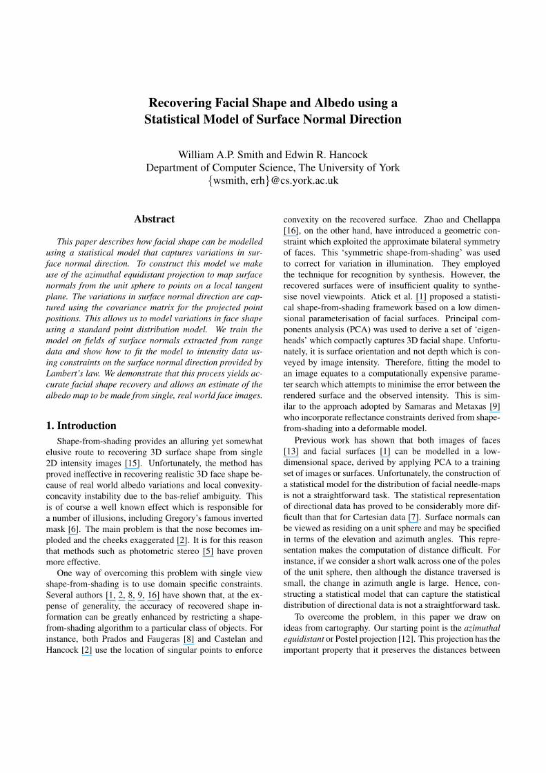
cos θ(i, j) cos θk(i, j) cos[φk(i, j) − φ(i, j)].Thus, in Figure 1, CP ′ is made equal to the arc CP for

all values of θ. The projected position of P , namely P ′,therefore lies at a distance θ from the centre of projectionand the direction of P ′ from the centre of the projection istrue. The equations for the inverse transformation from thetangent plane to the unit-sphere are

θk(i, j) = sin−1

{

cos c sin θ(i, j) −1

cyk(i, j) sin c cos θ(i, j)

}

φk(i, j) =φ(i, j) + tan−1 ψ(i, j)

θC O

PP'

Figure 1. The azimuthal equidistant projection

where

ψ(i, j) =

xk(i,j) sin c

c cos θ(i,j) cos c−yk(i,j) sin θ(i,j) sin cif θ(i, j) 6= ±π

2

−xk(i,j)yk(i,j) if θ(i, j) = π

2xk(i,j)yk(i,j) if θ(i, j) = −π

2

and c =√

xk(i, j)2 + yk(i, j)2.

2.1. Point Distribution Model

For each image location the transformed surface nor-mals from the K different training images are concate-nated and stacked to form two long-vectors of lengthK. For the pixel location indexed (i, j), the firstof these is the long vector with the transformed x-co-ordinates from the training images as components, i.e.Vx(i, j) = (x1(i, j), x2(i, j), ..., xK(i, j))T and the sec-ond long-vector has the y co-ordinate as its components,i.e. Vy(i, j) = (y1(i, j), y2(i, j), ..., yK(i, j))T . Since theazimuthal equidistant projection involves centering the lo-cal co-ordinate system, the coordinates corresponding to themean direction are (0, 0) at each image location. Hence,the long-vector corresponding to the mean direction at eachimage location is zero. If the data is of dimensions Mrows and N columns, then there are M × N pairs ofsuch long-vectors. The long vectors are ordered accordingto the raster scan (left-to-right and top-to-bottom) and areused as the columns of the K × (2MN) data-matrix D =(Vx(1, 1)|Vy(1, 1)| . . . |Vx(M,N)|Vy(M,N)). The co-variance matrix for the long-vectors is the (2MN) ×(2MN) matrix L = 1

KD

TD. We follow Atick et al. [1]

and use the numerically efficient method of Sirovich [10] tocompute the eigenvectors of L. Accordingly, we constructthe matrix L = 1

KDD

T . The eigenvectors ei of L can beused to find the eigenvectors ei of L using ei = D

Tei.

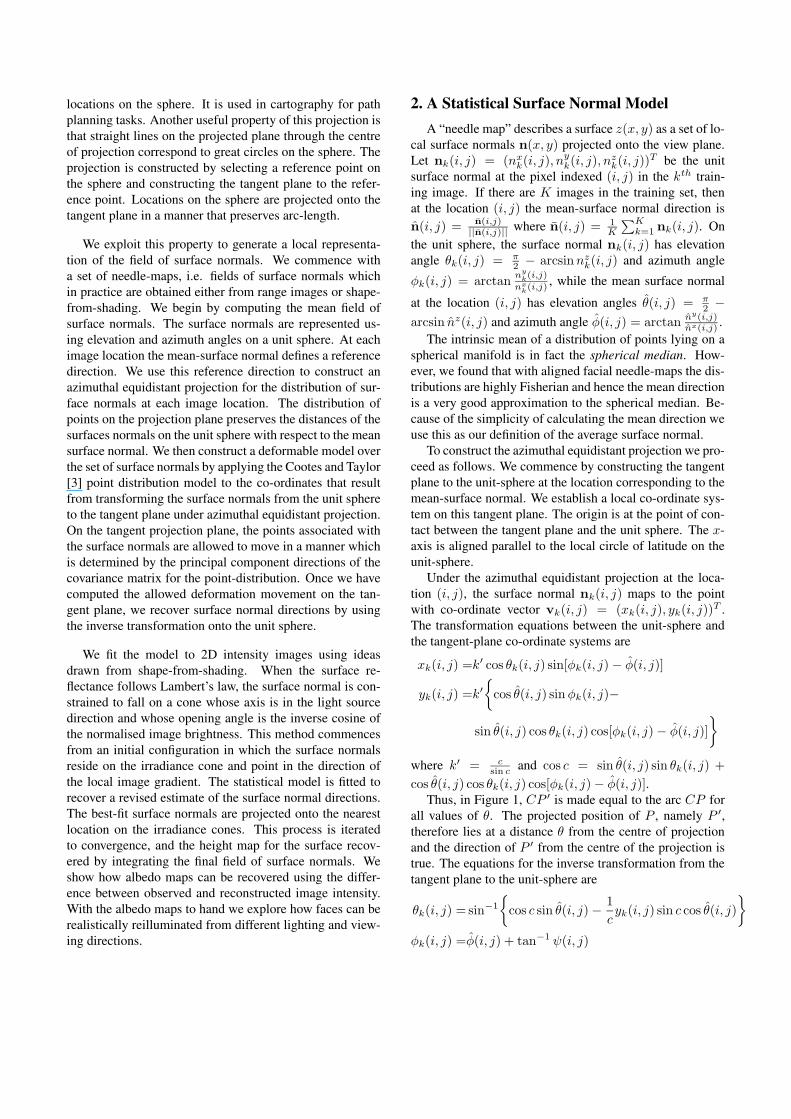
Figure 2 illustrates the process used in constructing ourmodel. On the left a distribution of surface normals at onepixel in a model is shown as points on the unit sphere. Onthe right the azimuthal equidistant projection of the points isshown with the mean point as the centre of projection. Thefirst PCA axis is shown by the line labelled PCA1. Thisline corresponds to a great circle on the sphere through the

Figure 2. Projection of points on the unit sphere topoints on the tangent plane at the mean point

mean direction which minimises the spherical distance toeach point.

The first K eigenvalues λi of L are given by the eigen-values λi of L, the remainder are zero. We may considersmall scale variation as noise. Hence, we need only retainS eigenmodes to retain p percent of the model variance. Wechoose S using

∑S

i=1 λi ≥ p100

∑K

i=1 λi. We deform theazimuthal equidistant point projections in the directions de-fined by the matrix P = (e1|e2| . . . |eS) formed from theleading S principal eigenvectors.

The simplest manner in which to fit the model to animage of a face is to use a shape-from-shading algorithmto extract a field of surface normals from the image. Theobserved field of surface normals undergoes an azimuthalequidistant projection at each point and the resulting coor-dinates are stacked to form a vector vk as described above.A vector of parameters b describing the needle-map in themodel parameter space is given by projecting the vector vk

onto the model eigenspace, b = PTvk. This parameter

vector will represent the closest needle-map in the modelspace and hence, if the model is trained on ground truthdata, will help resolve errors in the input needle-map. How-ever, given the difficulties inherent in robust needle-maprecovery from real world images, this projection approachdoes not work well in practice. In the next section we de-scribe an approach to fitting the model to image data whichexploits the constraint provided by the model with greatlyimproved results.

3. Fitting the Model to Intensity Images

We may exploit the statistical constraint provided by themodel in the process of fitting the model to an intensity im-age and thus help resolve the ambiguity in the shape-from-shading process. We do this using an iterative approachwhich can be posed as that of recovering the best-fit field ofsurface normals from the statistical model, subject to con-straints provided by the image irradiance equation.

If I is the measured image brightness, then according toLambert’s law I = n.s, where s is the light source direction.In general, the surface normal n can not be recovered froma single brightness measurement since it has two degrees of

freedom corresponding to the elevation and azimuth angleson the unit sphere. In the Worthington and Hancock [14]iterative shape-from-shading framework, data-closeness isensured by constraining the recovered surface normal to lieon the reflectance cone whose axis is aligned with the light-source vector s and whose opening angle is α = arccos I .At each iteration the surface normal is free to move to anoff-cone position subject to smoothness or curvature consis-tency constraints. However, the hard irradiance constraint isre-imposed by rotating each surface normal back to its clos-est on-cone position. This process ensures that the recov-ered field of surface normals satisfies the image irradianceequation after every iteration.

Suppose that n′l(i, j) is an off-cone surface normal at

iteration l of the algorithm. The update equation is there-fore n

l+1(i, j) = Θn′l(i, j) where Θ is a rotation matrix

computed from the apex angle α and the angle betweenn′l(i, j) and the light source direction s. To restore the

surface normal to the closest on-cone position it must berotated by an angle θ = α − arccos

[

n′l(i, j).s

]

about theaxis (u, v, w)T = n

′l(i, j) × s. Hence, the rotation matrixis

Θ =

c+ u2c′ −ws+ uvc′ vs+ uwc′

ws+ uvc′ c+ v2c′ −us+ vwc′

−vs+ uwc′ us+ vwc′ c+ w2c′

where c = cos(θ), c′ = 1 − c and s = sin(θ).The framework is initialised by placing the surface nor-

mals on their reflectance cones such that they are aligned inthe direction opposite to that of the local image gradient.

Our approach to fitting the model to intensity imagesuses the fields of surface normals estimated using the ge-ometric shape-from-shading method described above. Thisis an iterative process in which we interleave the process offitting the statistical model to the current field of estimatedsurface normals, and then re-enforcing the data-closenessconstraint provided by Lambert’s law by mapping the sur-face normals back onto their reflectance cones. The algo-rithm can be summarised as follows:

1. Initialise the field of surface normals n.2. Each normal in the estimated field n undergoes an az-

imuthal equidistant projection to give a vector of trans-formed coordinates v.

3. The best fit to the vector of transformed coordinates isv′ = PP

Tv.

4. Using the inverse azimuthal equidistant projection findn′ from v

′.5. Find n

′′ by rotating n′ using n

′′(i, j) = Θn′(i, j).

6. Stop if the difference between n and n′′ indicates con-

vergence.7. Make n = n

′′ and return to step 2.

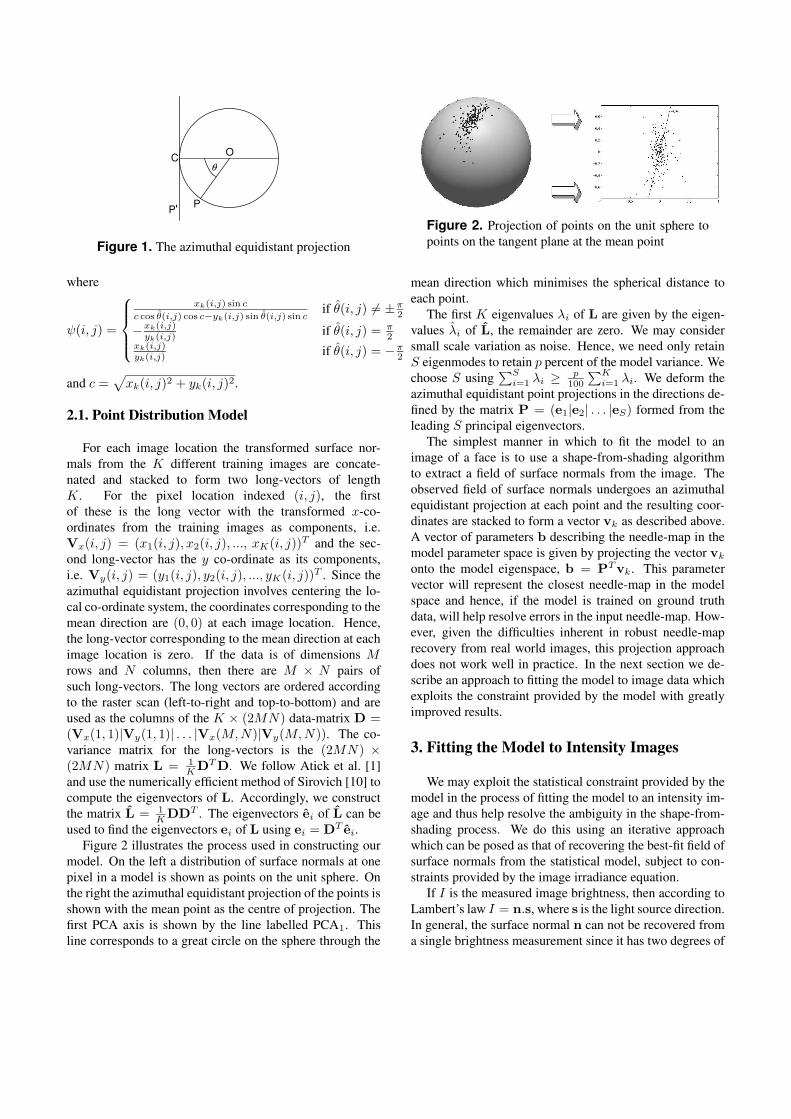
Figure 3. Angular difference between n′ and n

′′

3.1. Albedo Estimation

Upon convergence we output n′′, which satisfies the

data-closeness constraint. However, given the variation inalbedo in real world facial images, this may not be desir-able. In Figure 3 we show the angular change as data-closeness is restored to a typical final best fit needle map,i.e. the angular difference between n

′ and n′′. From the

plot it is clear that the changes are almost solely due to thevariation in albedo at the eyes, eye-brows and lips. Asidefrom these regions there is very little change in surface nor-mal direction, indicating the needle map has converged to asolution which satisfies the data-closeness constraint exceptin regions of actual variation in albedo.

For this reason we may choose to output n′ and an esti-

mate of the albedo map. In other words we relax the data-closeness constraint at the final iteration and use the dif-ferences between observed and reconstructed image bright-ness to account for albedo variations. If the final best-fitfield of surface normals is reilluminated using a Lamber-tian reflectance model, then the predicted image brightnessis given by I(i, j) = ρ(i, j)[s.n′(i, j)] where ρ(i, j) is thealbedo at position (i, j). Since I , s, and n

′ are all knownwe can estimate the albedo at each pixel using the formula:ρ(i, j) = I(i,j)

s.n′(i,j) .

4. Experiments

In this Section we present experiments with our method.We commence by investigating the results of fitting themodel to intensity data, and show the surface height datathat can be reconstructed from the fitted fields of surfacenormals. Second, we show how the model can be used toestimate a stable albedo map under varying illumination.Finally, we illustrate how the fitted models can be used tosynthesise novel facial views.

We train the statistical model using surface normals ex-tracted from range images of faces. The method could betrained on surface normal data delivered by shape-from-shading, but this is generally less reliable. We used 200range images of male and female subjects with neutral ex-pressions. 142 dimensions were used in the model to re-tain 95% of the variance. The images used in this studycome from the Yale-B database [5]. In the images the faces

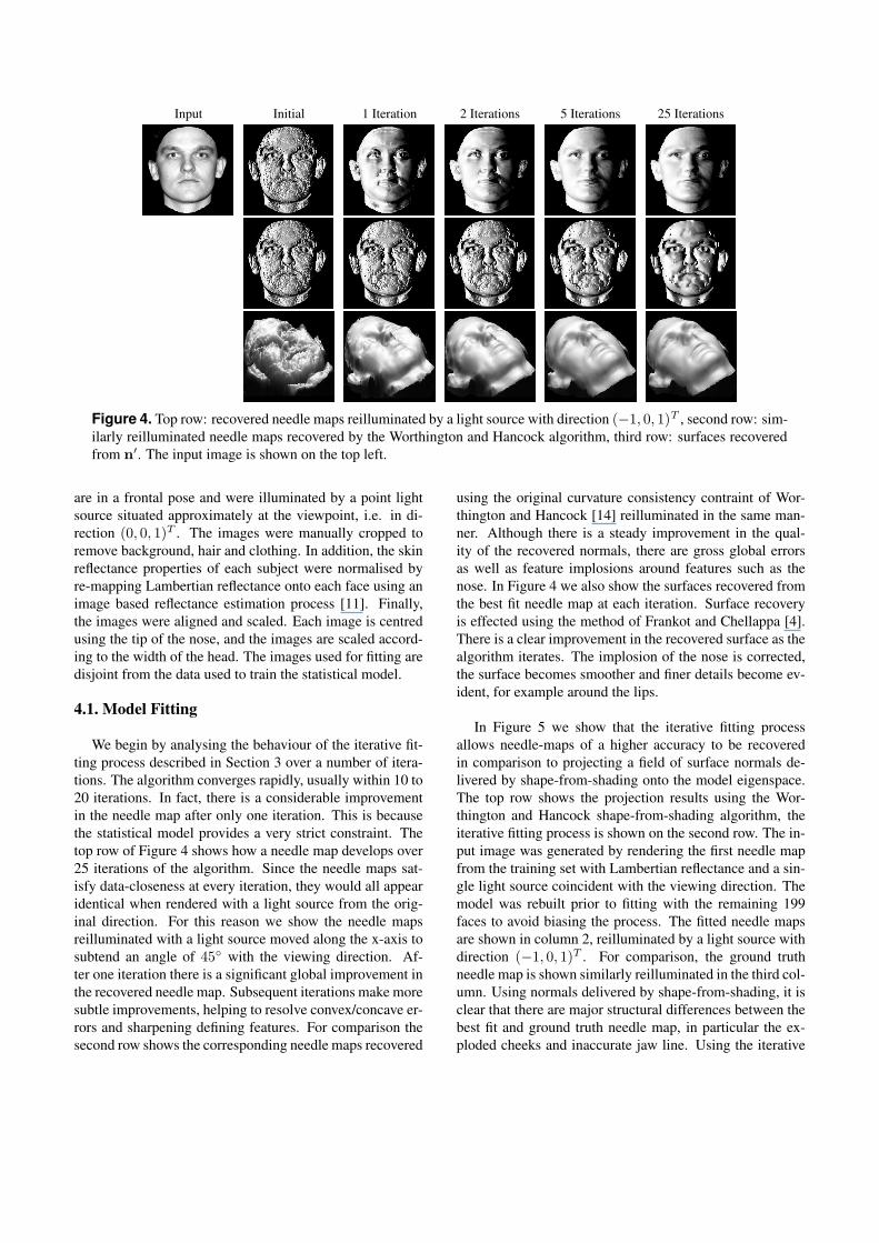
Input Initial 1 Iteration 2 Iterations 5 Iterations 25 Iterations

Figure 4. Top row: recovered needle maps reilluminated by a light source with direction (−1, 0, 1)T , second row: sim-ilarly reilluminated needle maps recovered by the Worthington and Hancock algorithm, third row: surfaces recoveredfrom n

′. The input image is shown on the top left.

are in a frontal pose and were illuminated by a point lightsource situated approximately at the viewpoint, i.e. in di-rection (0, 0, 1)T . The images were manually cropped toremove background, hair and clothing. In addition, the skinreflectance properties of each subject were normalised byre-mapping Lambertian reflectance onto each face using animage based reflectance estimation process [11]. Finally,the images were aligned and scaled. Each image is centredusing the tip of the nose, and the images are scaled accord-ing to the width of the head. The images used for fitting aredisjoint from the data used to train the statistical model.

4.1. Model Fitting

We begin by analysing the behaviour of the iterative fit-ting process described in Section 3 over a number of itera-tions. The algorithm converges rapidly, usually within 10 to20 iterations. In fact, there is a considerable improvementin the needle map after only one iteration. This is becausethe statistical model provides a very strict constraint. Thetop row of Figure 4 shows how a needle map develops over25 iterations of the algorithm. Since the needle maps sat-isfy data-closeness at every iteration, they would all appearidentical when rendered with a light source from the orig-inal direction. For this reason we show the needle mapsreilluminated with a light source moved along the x-axis tosubtend an angle of 45◦ with the viewing direction. Af-ter one iteration there is a significant global improvement inthe recovered needle map. Subsequent iterations make moresubtle improvements, helping to resolve convex/concave er-rors and sharpening defining features. For comparison thesecond row shows the corresponding needle maps recovered

using the original curvature consistency contraint of Wor-thington and Hancock [14] reilluminated in the same man-ner. Although there is a steady improvement in the qual-ity of the recovered normals, there are gross global errorsas well as feature implosions around features such as thenose. In Figure 4 we also show the surfaces recovered fromthe best fit needle map at each iteration. Surface recoveryis effected using the method of Frankot and Chellappa [4].There is a clear improvement in the recovered surface as thealgorithm iterates. The implosion of the nose is corrected,the surface becomes smoother and finer details become ev-ident, for example around the lips.

In Figure 5 we show that the iterative fitting processallows needle-maps of a higher accuracy to be recoveredin comparison to projecting a field of surface normals de-livered by shape-from-shading onto the model eigenspace.The top row shows the projection results using the Wor-thington and Hancock shape-from-shading algorithm, theiterative fitting process is shown on the second row. The in-put image was generated by rendering the first needle mapfrom the training set with Lambertian reflectance and a sin-gle light source coincident with the viewing direction. Themodel was rebuilt prior to fitting with the remaining 199faces to avoid biasing the process. The fitted needle mapsare shown in column 2, reilluminated by a light source withdirection (−1, 0, 1)T . For comparison, the ground truthneedle map is shown similarly reilluminated in the third col-umn. Using normals delivered by shape-from-shading, it isclear that there are major structural differences between thebest fit and ground truth needle map, in particular the ex-ploded cheeks and inaccurate jaw line. Using the iterative

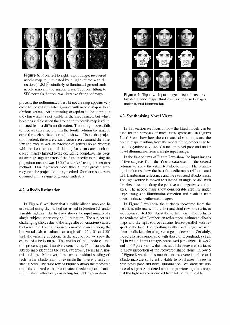
Figure 5. From left to right: input image, recoveredneedle-map reilluminated by a light source with di-rection (-1,0,1)T , similarly reilluminated ground truthneedle map and the angular error. Top row: fitting toSFS normals, bottom row: iterative fitting to image.

process, the reilluminated best fit needle map appears veryclose to the reilluminated ground truth needle map with noobvious errors. An interesting exception is the dimple inthe chin which is not visible in the input image, but whichbecomes visible when the ground truth needle map is reillu-minated from a different direction. The fitting process failsto recover this structure. In the fourth column the angularerror for each surface normal is shown. Using the projec-tion method, there are clearly large errors around the nose,jaw and eyes as well as evidence of general noise, whereaswith the iterative method the angular errors are much re-duced, mainly limited to the occluding boundary. The over-all average angular error of the fitted needle map using theprojection method was 13.25◦ and 3.93◦ using the iterativemethod. This represents more than 3 times greater accu-racy than the projection fitting method. Similar results wereobtained with a range of ground truth data.

4.2. Albedo Estimation

In Figure 6 we show that a stable albedo map can beestimated using the method described in Section 3.1 undervariable lighting. The first row shows the input images of asingle subject under varying illumination. The subject is achallenging choice due to the large albedo variations causedby facial hair. The light source is moved in an arc along thehorizontal axis to subtend an angle of −25◦, 0◦ and 25◦

with the viewing direction. In the second row we show theestimated albedo maps. The results of the albedo estima-tion process appear intuitively convincing. For instance, thealbedo map identifies the eyes, eyebrows, facial hair, nos-trils and lips. Moreover, there are no residual shading ef-fects in the albedo map, for example the nose is given con-stant albedo. The third row of Figure 6 shows the recoverednormals rendered with the estimated albedo map and frontalillumination, effectively correcting for lighting variation.

Figure 6. Top row: input images, second row: es-timated albedo maps, third row: synthesised imagesunder frontal illumination.

4.3. Synthesising Novel Views

In this section we focus on how the fitted models can beused for the purposes of novel view synthesis. In Figures7 and 8 we show how the estimated albedo maps and theneedle maps resulting from the model fitting process can beused to synthesise views of a face in novel pose and undernovel illumination from a single input image.

In the first column of Figure 7 we show the input imagesof five subjects from the Yale-B database. In the secondcolumn we show the estimated albedo maps. The remain-ing 4 columns show the best fit needle maps reilluminatedwith Lambertian reflectance and the estimated albedo maps.The light source is moved to subtend an angle of 45◦ withthe view direction along the positive and negative x and y-axes. The needle maps show considerable stability underlarge changes in illumination direction and result in nearphoto-realistic synthesised images.

In Figure 8 we show the surfaces recovered from thebest fit needle maps. In the first and third rows the surfacesare shown rotated 30◦ about the vertical axis. The surfacesare rendered with Lambertian reflectance, estimated albedomaps and the light source remains fronto-parallel with re-spect to the face. The resulting synthesised images are nearphoto-realistic under a large change in viewpoint. Certainly,the results are comparable with those of Georghiades et al.[5] in which 7 input images were used per subject. Rows 2and 4 of Figure 8 show the meshes of the recovered surfacesto allow inspection of the recovered shape alone. In row 5of Figure 8 we demonstrate that the recovered surface andalbedo map are sufficiently stable to synthesise images inboth novel pose and novel illumination. We show the sur-face of subject 8 rendered as in the previous figure, exceptthat the light source is circled from left to right profile.

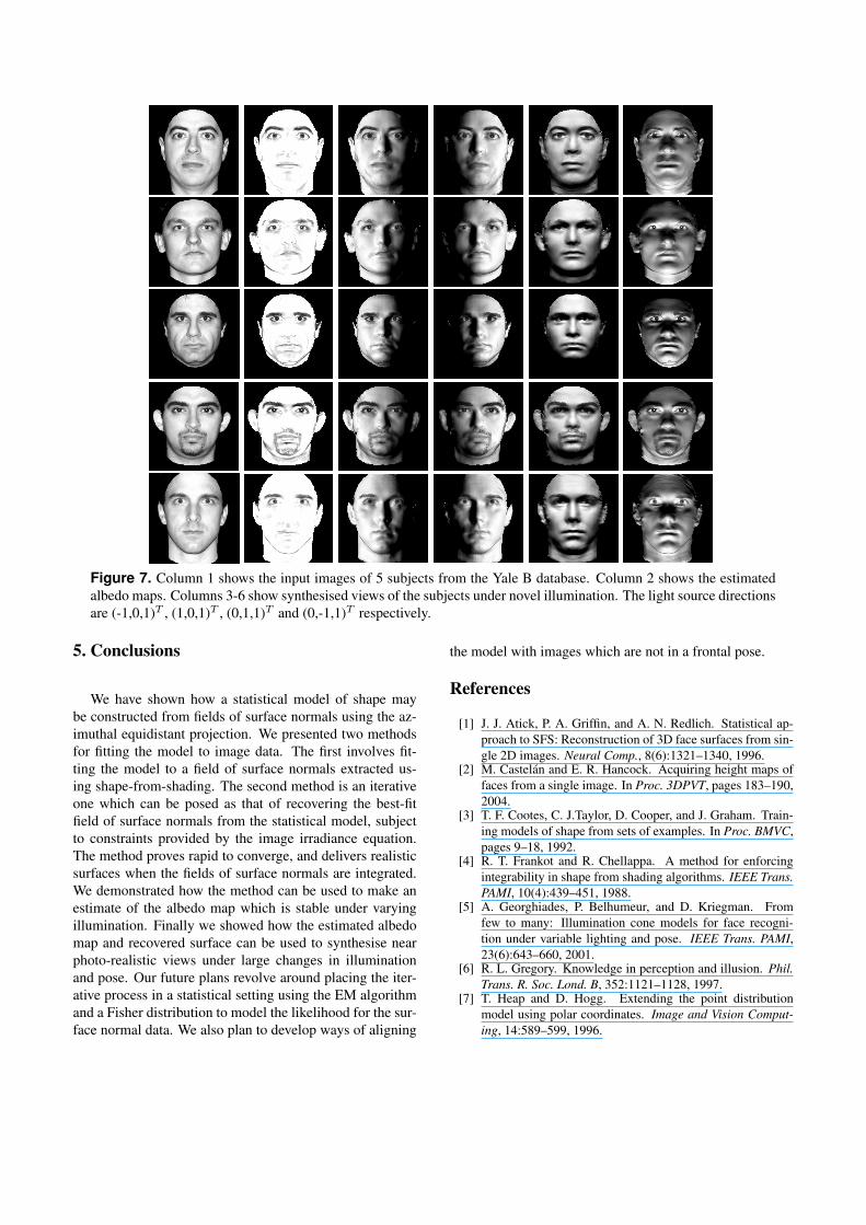
Figure 7. Column 1 shows the input images of 5 subjects from the Yale B database. Column 2 shows the estimatedalbedo maps. Columns 3-6 show synthesised views of the subjects under novel illumination. The light source directionsare (-1,0,1)T , (1,0,1)T , (0,1,1)T and (0,-1,1)T respectively.

5. Conclusions

We have shown how a statistical model of shape maybe constructed from fields of surface normals using the az-imuthal equidistant projection. We presented two methodsfor fitting the model to image data. The first involves fit-ting the model to a field of surface normals extracted us-ing shape-from-shading. The second method is an iterativeone which can be posed as that of recovering the best-fitfield of surface normals from the statistical model, subjectto constraints provided by the image irradiance equation.The method proves rapid to converge, and delivers realisticsurfaces when the fields of surface normals are integrated.We demonstrated how the method can be used to make anestimate of the albedo map which is stable under varyingillumination. Finally we showed how the estimated albedomap and recovered surface can be used to synthesise nearphoto-realistic views under large changes in illuminationand pose. Our future plans revolve around placing the iter-ative process in a statistical setting using the EM algorithmand a Fisher distribution to model the likelihood for the sur-face normal data. We also plan to develop ways of aligning

the model with images which are not in a frontal pose.

References

[1] J. J. Atick, P. A. Griffin, and A. N. Redlich. Statistical ap-proach to SFS: Reconstruction of 3D face surfaces from sin-gle 2D images. Neural Comp., 8(6):1321–1340, 1996.

[2] M. Castelan and E. R. Hancock. Acquiring height maps offaces from a single image. In Proc. 3DPVT, pages 183–190,2004.

[3] T. F. Cootes, C. J.Taylor, D. Cooper, and J. Graham. Train-ing models of shape from sets of examples. In Proc. BMVC,pages 9–18, 1992.

[4] R. T. Frankot and R. Chellappa. A method for enforcingintegrability in shape from shading algorithms. IEEE Trans.PAMI, 10(4):439–451, 1988.

[5] A. Georghiades, P. Belhumeur, and D. Kriegman. Fromfew to many: Illumination cone models for face recogni-tion under variable lighting and pose. IEEE Trans. PAMI,23(6):643–660, 2001.

[6] R. L. Gregory. Knowledge in perception and illusion. Phil.Trans. R. Soc. Lond. B, 352:1121–1128, 1997.

[7] T. Heap and D. Hogg. Extending the point distributionmodel using polar coordinates. Image and Vision Comput-ing, 14:589–599, 1996.

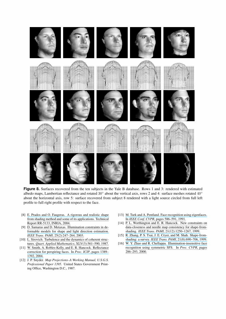
Figure 8. Surfaces recovered from the ten subjects in the Yale B database. Rows 1 and 3: rendered with estimatedalbedo maps, Lambertian reflectance and rotated 30◦ about the vertical axis, rows 2 and 4: surface meshes rotated 40◦

about the horizontal axis, row 5: surface recovered from subject 8 rendered with a light source circled from full leftprofile to full right profile with respect to the face.

[8] E. Prados and O. Faugeras. A rigorous and realistic shapefrom shading method and some of its applications. TechnicalReport RR-5133, INRIA, 2004.

[9] D. Samaras and D. Metaxas. Illumination constraints in de-formable models for shape and light direction estimation.IEEE Trans. PAMI, 25(2):247–264, 2003.

[10] L. Sirovich. Turbulence and the dynamics of coherent struc-tures. Quart. Applied Mathematics, XLV(3):561–590, 1987.

[11] W. Smith, A. Robles-Kelly, and E. R. Hancock. Reflectancecorrection for perspiring faces. In Proc. ICIP, pages 1389–1392, 2004.

[12] J. P. Snyder. Map Projections–A Working Manual, U.S.G.S.Professional Paper 1395. United States Government Print-ing Office, Washington D.C., 1987.

[13] M. Turk and A. Pentland. Face recognition using eigenfaces.In IEEE Conf. CVPR, pages 586–591, 1991.

[14] P. L. Worthington and E. R. Hancock. New constraints ondata-closeness and needle map consistency for shape-from-shading. IEEE Trans. PAMI, 21(12):1250–1267, 1999.

[15] R. Zhang, P. S. Tsai, J. E. Cryer, and M. Shah. Shape-from-shading: a survey. IEEE Trans. PAMI, 21(8):690–706, 1999.

[16] W. Y. Zhao and R. Chellappa. Illumination-insensitive facerecognition using symmetric SFS. In Proc. CVPR, pages286–293, 2000.