Embed Size (px)
Citation preview
Reducing Belief Revision to Circumscription
(and viceversa) ?
Paolo Liberatore and Marco Schaerf 1
Dipartimento di Informatica e Sistemistica
Universita di Roma “La Sapienza”
via Salaria 113, I-00198 Roma, Italy
email: {liberatore,schaerf}@dis.uniroma1.it
Abstract
Nonmonotonic formalisms and belief revision operators have been introduced as useful
tools to describe and reason about evolving scenarios. Both approaches have been proven
effective in a number of different situations. However, little is known about their relation-
ship. Previous work by Winslett has shown some correlations between a specific operator
and circumscription. In this paper we greatly extend Winslett’s work by establishing new
relations between circumscription and a large number of belief revision operators. This high-
lights similarities and differences between these formalisms. Furthermore, these connections
provide us with the possibility of importing results in one field into the other one.
Keywords: Knowledge Representation, Circumscription, Belief Revision, Computational
Complexity.
? Extended and revised version of [LS95].1 Work partially supported by ASI (Italian Space Agency).
Article published in Artificial Intelligence Journal. 93 (2002) 1–0
1 Introduction
During the last years, many formalisms have been proposed in the AI literature
to model commonsense reasoning. Particular emphasis has been put in the formal
modeling of a distinct feature of commonsense reasoning, that is, its nonmonotonic
nature. The AI goal of providing a logic model of human agents’ capability of reasoning
in the presence of incomplete or contradictory information has proven to be a very
hard one. Nevertheless, many important formalisms have been put forward in the
literature.
Two main approaches have been proposed to handle the nonmonotonic aspects of
commonsense reasoning. The first one deals with this problem, by defining a new
logic equipped with a nonmonotonic consequence operator. Important examples of
this approach are default logic proposed in [Rei80] and circumscription introduced in
[McC80]. The second one relies on preserving a classical (monotonic) inference opera-
tor, but introduces a revision operator that accommodates a new piece of information
into an existing body of knowledge. Specific revision operators have been introduced,
among the others, in [Gin86] and in [Dal88]. A general framework for revision has
been proposed by Alchourron, Gardenfors and Makinson in [AGfM85,Gar88]. A close
variant of revision is update. The general framework for update has been studied in
[KM89,KM91a] and specific operators have been proposed in [Win90] and [For89].
As pointed out by Winslett in [Win90], the large variety of candidate semantics for
belief revision and update varies widely in motivations, goals and area of application.
It is generally believed that there is no “best” method and that each one is suited for
a particular domain of application.
In this paper we investigate the relationship between circumscription and many op-
erators for belief revision and update. A first study of these relations has been done
2
in [Win89], where she relates her operator to circumscription. We expand her results
showing similar connections between several other belief revision operators and cir-
cumscription. To this end, we also introduce a variant of circumscription based on
cardinality, rather than set-containment.
The established correlations highlight the relations between the two fields. More-
over, as side benefits, they provide us with the opportunity to import results in
one field into the other one. A practical result is the possibility of directly using
algorithms developed for circumscription also for belief revision. In the last years,
many algorithms for circumscription have appeared in the literature (see, for exam-
ple, [Gin89,Prz89,NNS95]), while, to the best of our knowledge, only Winslett in
[Win90] has proposed an algorithm for belief revision. Using our reductions, it is pos-
sible to reduce a reasoning problem of belief revision into one in circumscription, thus
taking advantage of the large number of algorithms and reasoning systems already
developed.
In this paper we focus our attention on propositional languages, since some of the be-
lief revision operators have only been defined in this setting. However, in Section 9 we
briefly explain how and when our results also apply to full first-order circumscription
and belief revision.
The paper is organized as follows: In Section 2 we recall some key definitions and
results for belief revision and circumscription, introduce a variant of circumscription
(NCIRC), define the kind of relations we want to establish and explain the notation
used throughout the following sections. In Sections 3, 4, 5 and 6 we show the main
relations between the various kinds of revision operators and circumscription, while
in Section 7 we show relations and reductions between the various operators. In
Section 8 we focus on syntactically-restricted knowledge bases. Section 9 discusses
possible applications of our results with particular attention to the computational
complexity analysis. While in Section 10 we draw some conclusions. Finally, in the
3
appendices we have the proofs of most theorems and a brief description of some
complexity classes used for some of the results.
2 Preliminaries
In this section we (very briefly) present the background and terminology needed
to understand the results presented later in the paper. For the sake of simplicity,
throughout this paper we restrict our attention to a (finite) propositional language.
In Section 9 we briefly discuss how these results also apply to full first-order languages.
The alphabet of a propositional formula α is the set of all propositional atoms oc-
curring in it and is denoted by V (α). Formulae are built over a finite alphabet of
propositional letters using the usual connectives ¬ (not), ∨ (or) and ∧ (and). Ad-
ditional connectives are used as shorthands, α → β denotes ¬α ∨ β, α ≡ β is a
shorthand for (α ∧ β) ∨ (¬α ∧ ¬β).
An interpretation of a formula is a truth assignment to the atoms of its alphabet.
A model M of a formula F is an interpretation that satisfies F (written M |= F ).
Interpretations and models of propositional formulae will be denoted as sets of atoms
(those which are mapped into 1). A theory T is a set of formulae. An interpretation
is a model of a theory if it is a model of every formula of the theory. Given a theory T
and a formula F we say that T entails F , written T |= F , if F is true in every model
of T . Given a propositional formula or a theory T , we denote with M(T ) the set of
its models. We say that T is consistent, written T 6|= ⊥, if M(T ) is non-empty.
4
2.1 Belief Revision and Update
Belief revision is concerned with the modeling of accommodating a new piece of
information (the revising formula) into an existing body of knowledge (the knowledge
base), where the two might contradict each other. A slightly different perspective is
taken by knowledge update. An analysis of the differences between belief revision
and update is out of the scope of this paper, for an interesting discussion we refer
the reader to the work [KM91a]. We assume that both the revising formula and the
knowledge base can be either a single formula or a theory.
In the literature, the first formal studies on the principles of belief revision have been
presented by Alchourron, Gardenfors and Makinson in [AGfM85,Gar88]. In these
papers they present a set of postulates that all revision operators should satisfy.
These postulates, known as the AGM postulates, assume that the revision operator
applies to a deductively-closed set of formulae. In order to make the presentation more
homogeneous, we present the reformulation of these postulates where the revision
operator applies to propositional formulae. More precisely, we denote with K the
knowledge base (that is the existing logical theory), with A the revising formula
(that is the new information) and with ∗ the revision operator. This formulation has
been presented by Katsuno and Mendelzon in [KM91b], where they prove this set of
postulates equivalent to the original one.
Thus, the AGM postulates for (finite) propositional knowledge bases are:
AGM1 K ∗ A implies A.
AGM2 If K ∧ A is satisfiable then K ∗ A ≡ K ∧ A.
AGM3 If A is satisfiable then K ∗ A is also satisfiable.
AGM4 If K1 ≡ K2 and A1 ≡ A2 then K1 ∗ A1 ≡ K2 ∗ A2.
AGM5 (K ∗ A) ∧B implies K ∗ (A ∧B).
5
AGM6 If (K ∗ A) ∧B is satisfiable then K ∗ (A ∧B) implies (K ∗ A) ∧B.
The intuitive meaning of the postulates is simple to understand. AGM1 states that
the new information A is always retained in the revision. AGM2 postulates that, if no
consistency arises, A is simply added to K. AGM3 states that inconsistency cannot be
introduced unless A is inconsistent. Furthermore, because of AGM4 the revision op-
erator obeys the Principle of Irrelevance of Syntax and postulates AGM5 and AGM6
impose constraints on the behavior of revision in the presence of conjunctions.
Katsuno and Mendelzon in [KM91b] have shown that, to any revision operator satis-
fying AGM1-AGM6, corresponds a family of reflexive, transitive and total orderings
over the set of interpretations, one for each formula K. Given a revision ∗ and its
corresponding family of orderings, the following relation holds.
M(K ∗ A) = min(M(A),≤K) (1)
Any given ordering ≤K has the so-called property of faithfulness, that can be sum-
marized as follows:
(i) If I ∈M(K) then I ≤K J for any interpretation J .
(ii) If I ∈M(K) and J 6∈ M(K) then J ≤K I does not hold.
Roughly speaking, the models of M(K) are exactly the minimal elements of ≤K ,
and the other interpretations are ordered according to their distance from models of
K: given two models I and J , it holds I ≤K J if and only if I is considered more
plausible to an agent believing K. In this sense, achieving the principle of minimal
change, equation 1 means that the result of a revision is constituted by the models
of A that are closer to K.
We now recall the different approaches to revision and update, classifying them into
formula-based and model-based ones. A more thorough exposition can be found in
6
[EG92]. We use the following conventions: the expression card(S) denotes the car-
dinality of a set S, and symmetric difference between two sets S1, S2 is denoted by
S1∆S2. If S is a set of sets, ∩S denotes the set formed intersecting all sets of S, and
analogously ∪S for union; min⊆S denotes the subset of S containing only the mini-
mal (w.r.t. set inclusion) sets in S, while max⊆S denotes its maximal sets. Moreover,
we use the symbol ⊂ to denote strict containment, i.e. S1 ⊂ S2 if and only S1 ⊆ S2
and ∃a ∈ S2 such that a 6∈ S1.
Formula-based approaches operate on the formulae syntactically appearing in the
knowledge base K. Let C(K,A) be the set of the subsets of K that are consistent
with the revising formula A:
C(K,A) = {K ′ ⊆ K | K ′ ∪ {A} 6|= ⊥}
and let W (K, A) be the set of the maximal sets of C(K, A):
W (K, A) = max⊆C(K,A)
The set W (K,A) contains all the plausible subsets of K that we may retain when
inserting A.
SBR. In [FUV83] and in [Gin86], the revised knowledge base is defined as a set of
theories: K ∗SBR A.= {K ′∪{A} | K ′ ∈ W (K, A)}. That is, the result of revising K is
the set of all maximal subsets of K consistent with A, plus A. Logical consequence in
the revised knowledge base is defined as logical consequence in each of the theories,
i.e. K∗SBRA |= Q iff for all K ′ ∈ W (K,A), K ′∪{A} |= Q. In other words, Fagin et al.
and Ginsberg consider all sets in W (K, A) equally plausible and inference is defined
skeptically, i.e. Q must be a consequence of each set. For this reason, we term this
method as Skeptical Belief Revision (SBR). Note that K ∗SBR A can be equivalently
rewritten as∨
K′∈W (K,A) K ′.
7
Note that formula-based approaches are sensitive to the syntactic form of the theory.
That is, the revision with the same formula A of two logically equivalent theories K1
and K2, may yield different results, depending on the syntactic form of K1 and K2.
We illustrate this fact through an example.
Example 1 Consider K1 = {a, b}, K2 = {a, a → b} and A = ¬b. Clearly, K1 is
equivalent to K2. The only maximal subset of K1 consistent with A is {a}, while there
are two maximal consistent subsets of K2, that are {a} and {a → b}.
Thus, K1 ∗SBR A = {a,¬b} while K2 ∗SBR A = {(a ∧ ¬b) ∨ ((a → b) ∧ ¬b)} that is
equivalent to {¬b}.
Model-based approaches instead operate by selecting the models of A on the basis of
some notion of proximity to the models of K. Model-based approaches assume K
to be a single formula, if K is a set of formulae it is implicitly interpreted as the
conjunction of all the elements. Many notions of proximity have been defined in the
literature. We distinguish them between pointwise proximity and global proximity.
We first recall approaches in which proximity between models of A and models of
K is computed pointwise w.r.t. each model of K. That is, they select models of K
one-by-one and, for each one, choose the closest model of A. These approaches are
considered as more suitable for knowledge update [KM91a]. Let M be a model, we
define µ(M,A) as the set containing the minimal differences (w.r.t. set inclusion)
between each model of A and the given M ; more formally:
µ(M, A).= min⊆{M∆N | N ∈M(A)}
We also use the notation kM,A to denote the minimum cardinality of sets in µ(M,A),
i.e. kM,A = min(n|n = |S|, S ∈ µ(M,A)).
Winslett. The work [Win90] defines the models of the updated knowledge base as
8
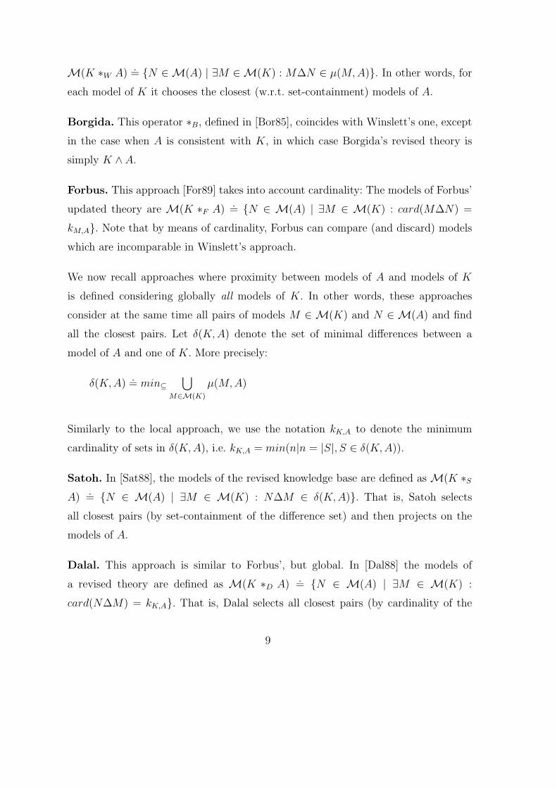
M(K ∗W A).= {N ∈ M(A) | ∃M ∈ M(K) : M∆N ∈ µ(M, A)}. In other words, for
each model of K it chooses the closest (w.r.t. set-containment) models of A.
Borgida. This operator ∗B, defined in [Bor85], coincides with Winslett’s one, except
in the case when A is consistent with K, in which case Borgida’s revised theory is
simply K ∧ A.
Forbus. This approach [For89] takes into account cardinality: The models of Forbus’
updated theory are M(K ∗F A).= {N ∈ M(A) | ∃M ∈ M(K) : card(M∆N) =
kM,A}. Note that by means of cardinality, Forbus can compare (and discard) models
which are incomparable in Winslett’s approach.
We now recall approaches where proximity between models of A and models of K
is defined considering globally all models of K. In other words, these approaches
consider at the same time all pairs of models M ∈ M(K) and N ∈ M(A) and find
all the closest pairs. Let δ(K, A) denote the set of minimal differences between a
model of A and one of K. More precisely:
δ(K,A).= min⊆
⋃
M∈M(K)
µ(M,A)
Similarly to the local approach, we use the notation kK,A to denote the minimum
cardinality of sets in δ(K, A), i.e. kK,A = min(n|n = |S|, S ∈ δ(K, A)).
Satoh. In [Sat88], the models of the revised knowledge base are defined as M(K ∗S
A).= {N ∈ M(A) | ∃M ∈ M(K) : N∆M ∈ δ(K,A)}. That is, Satoh selects
all closest pairs (by set-containment of the difference set) and then projects on the
models of A.
Dalal. This approach is similar to Forbus’, but global. In [Dal88] the models of
a revised theory are defined as M(K ∗D A).= {N ∈ M(A) | ∃M ∈ M(K) :
card(N∆M) = kK,A}. That is, Dalal selects all closest pairs (by cardinality of the
9
difference set) and then projects on the models of A.
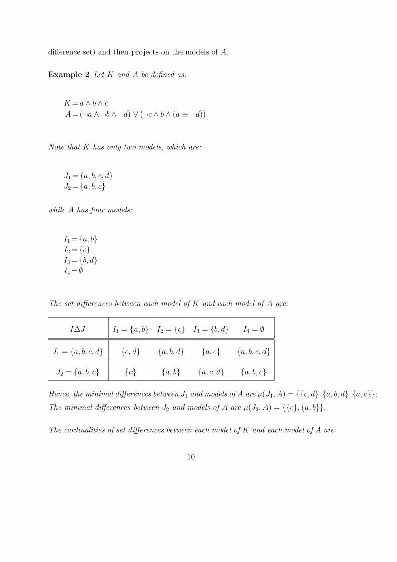
Example 2 Let K and A be defined as:
K = a ∧ b ∧ c
A = (¬a ∧ ¬b ∧ ¬d) ∨ (¬c ∧ b ∧ (a ≡ ¬d))
Note that K has only two models, which are:
J1 = {a, b, c, d}J2 = {a, b, c}
while A has four models:
I1 = {a, b}I2 = {c}I3 = {b, d}I4 = ∅
The set differences between each model of K and each model of A are:
I∆J I1 = {a, b} I2 = {c} I3 = {b, d} I4 = ∅
J1 = {a, b, c, d} {c, d} {a, b, d} {a, c} {a, b, c, d}
J2 = {a, b, c} {c} {a, b} {a, c, d} {a, b, c}
Hence, the minimal differences between J1 and models of A are µ(J1, A) = {{c, d}, {a, b, d}, {a, c}};The minimal differences between J2 and models of A are µ(J2, A) = {{c}, {a, b}}.
The cardinalities of set differences between each model of K and each model of A are:
10
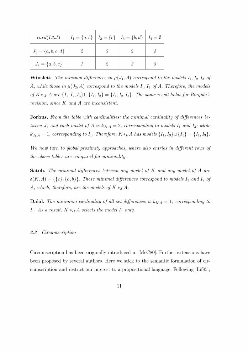
card(I∆J) I1 = {a, b} I2 = {c} I3 = {b, d} I4 = ∅
J1 = {a, b, c, d} 2 3 2 4
J2 = {a, b, c} 1 2 3 3
Winslett. The minimal differences in µ(J1, A) correspond to the models I1, I2, I3 of
A, while those in µ(J2, A) correspond to the models I1, I2 of A. Therefore, the models
of K ∗W A are {I1, I2, I3}∪{I1, I2} = {I1, I2, I3}. The same result holds for Borgida’s
revision, since K and A are inconsistent.
Forbus. From the table with cardinalities: the minimal cardinality of differences be-
tween J1 and each model of A is kJ1,A = 2, corresponding to models I1 and I3; while
kJ2,A = 1, corresponding to I1. Therefore, K∗F A has models {I1, I3}∪{I1} = {I1, I3}.
We now turn to global proximity approaches, where also entries in different rows of
the above tables are compared for minimality.
Satoh. The minimal differences between any model of K and any model of A are
δ(K, A) = {{c}, {a, b}}. These minimal differences correspond to models I1 and I2 of
A, which, therefore, are the models of K ∗S A.
Dalal. The minimum cardinality of all set differences is kK,A = 1, corresponding to
I1. As a result, K ∗D A selects the model I1 only.
2.2 Circumscription
Circumscription has been originally introduced in [McC80]. Further extensions have
been proposed by several authors. Here we stick to the semantic formulation of cir-
cumscription and restrict our interest to a propositional language. Following [Lif85],
11
we define:
Definition 1 Let T be a propositional formula, V (T ) = {x1, . . . , xn} its alphabet,
P , Q and Z disjoint sets of letters partitioning V (T ) (i.e. P ∪ Q ∪ Z = V (T )) and
M ∈ M(T ). M is called a (P,Z)-minimal model of T if there is no model N of T
such that N ∩Q = M ∩Q and (N ∩ P ) ⊂ (M ∩ P ).
Definition 2 The circumscription of T w.r.t. the three sets of letters P , Q and Z,
denoted as CIRC(T ; P, Q, Z), is an higher order formula whose set of models is the
set of all (P,Z)-minimal models of T , i.e. M |= CIRC(T ; P,Q, Z) iff M is a (P, Z)-
minimal model of T .
Informally, P is the set of letters we want to minimize, Q is the set of fixed letters,
while letters in Z are allowed to vary. Given two interpretations M and N , we use
the notation M ≤(P,Z) N to state that M is “(P,Z)-smaller” or equal than N , that
is (M ∩ Q) = (N ∩ Q) and (M ∩ P ) ⊆ (N ∩ P ). When we write M <(P,Z) N we
mean that M is strictly “(P,Z)-smaller” than N , that is (M ∩ Q) = (N ∩ Q) and
(M ∩ P ) ⊂ (N ∩ P ).
2.3 Cardinality-based Circumscription
The minimality criterion of circumscription is based on set-containment. We now in-
troduce, for propositional languages, a version of circumscription based on cardinality.
Definition 3 Let T be a propositional formula, V (T ) = {x1, . . . , xn} its alphabet,
P , Q and Z disjoint sets of letters partitioning V (T ) (i.e. P ∪ Q ∪ Z = V (T )) and
M ∈M(T ). M is called a (P, Z)-cardinality-minimal model of T if there is no model
N of T such that N ∩Q = M ∩Q and |N ∩ P | < |M ∩ P |.
Definition 4 The cardinality-based circumscription of T w.r.t. the three sets of let-
12
ters P , Q and Z, denoted as NCIRC(T ; P, Q,Z), is an higher order formula whose
set of models is the set of all (P,Z)-cardinality-minimal models of T , i.e. M |=NCIRC(T ; P, Q, Z) iff M is a (P, Z)-cardinality-minimal model of T .
In other words, I am preferring models with the least number of true letters of the
set P , rather than models with a least set of true letters. Given two interpretations
M and N , we use the notation M ¹(P,Z) N to state that M is “(P, Z)-cardinality-
smaller” than or equal to N , that is (M ∩Q) = (N ∩Q) and |(M ∩ P )| ≤ |(N ∩ P )|.Again, M ≺(P,Z) N denotes strict ordering. In order to better clarify the difference
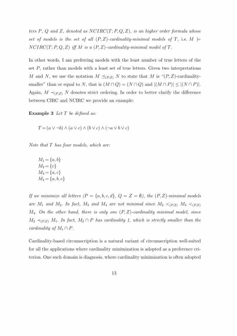
between CIRC and NCIRC we provide an example:
Example 3 Let T be defined as:
T = (a ∨ ¬b) ∧ (a ∨ c) ∧ (b ∨ c) ∧ (¬a ∨ b ∨ c)
Note that T has four models, which are:
M1 = {a, b}M2 = {c}M3 = {a, c}M4 = {a, b, c}
If we minimize all letters (P = {a, b, c, d}, Q = Z = ∅), the (P,Z)-minimal models
are M1 and M2. In fact, M3 and M4 are not minimal since M2 <(P,Z) M3 <(P,Z)
M4. On the other hand, there is only one (P,Z)-cardinality minimal model, since
M2 ≺(P,Z) M1. In fact, M2 ∩ P has cardinality 1, which is strictly smaller than the
cardinality of M1 ∩ P .
Cardinality-based circumscription is a natural variant of circumscription well-suited
for all the applications where cardinality minimization is adopted as a preference cri-
terion. One such domain is diagnosis, where cardinality minimization is often adopted
13
as the choice criterion.
2.4 Types of Reductions
In this paper we investigate whether circumscription and belief revision can be trans-
lated one into the other. To this end, we take into account various forms of reduc-
tions. Formally, a reduction from circumscription into belief revision is a pair of
functions f1 and f2 that take as input a 4-tuple T, P, Q, Z and produce two formulae
K = f1(T, P, Q, Z) and A = f2(T, P,Q, Z). Clearly, we want that the reduction pre-
serves the semantic content of the original knowledge base. Given a circumscriptive
theory CIRC(T ; P, Q,Z) and a revision operator ∗ we want that K = f1(T, P, Q, Z)
and A = f2(T, P, Q, Z) are such that the following relation holds:
{γ | CIRC(T ; P,Q, Z) |= γ} = {γ | K ∗ A |= γ}, (2)
γ being any formula in which only symbols of T occur. We call this property query
equivalence, and we say that if K ∗ A satisfies the above criterion then the result of
the reduction is query equivalent to CIRC(T ; P,Q, Z). Symmetrically, if given K and
A we find a T , P , Q and Z such that the relation (2) holds (where γ is a formula
using only symbols of K and A), we say that CIRC(T ; P, Q,Z) is query equivalent
to K ∗ A.
A tighter equivalence criterion we might look for is a form of equivalence characterized
by the following requirement
CIRC(T ; P, Q,Z) ≡ K ∗ A (3)
We call this property logical equivalence, and we say that if a pair of formulae K
and A is such that K ∗ A satisfies the above criterion it is logically equivalent to
14
CIRC(T ; P, Q, Z). Notice that if K∗A satisfies logical equivalence (3) it satisfies query
equivalence (2) as well, but not the other way around. Basically, query equivalence
(2) gives the possibility of introducing new propositional letters. This has definitely
an impact on the possibility of translating circumscription into belief revision, as we
will show. Symmetrically, if given K and A we find a T , P , Q and Z such that the
relation (3) holds (where γ is a formula using only symbols of K and A), we say that
CIRC(T ; P, Q, Z) is logically equivalent to K ∗ A.
The above properties do not take into account the computational cost of the reduc-
tions. This is far too general, in fact, unrestricted reductions are of little practical
interest and, furthermore since both circumscription and the belief revision opera-
tors can represent all boolean functions, unrestricted reductions always exist. For this
reason, we consider two restrictions on the cost of reductions: if the reduction can
be computed in polynomial time (i.e. both f1 and f2 can be computed in polynomial
time), we call it a poly-time reduction. On the other hand, if the size of the result of
the reduction is polynomial in the size of the inputs (i.e. the result of both f1 and f2
has size polynomial), we call it a poly-size reduction. Note that poly-size reductions
are more general than poly-time ones. In fact, all poly-time reductions are also poly-
size, while the contrary does not necessarily hold. While poly-time reductions are of
obvious interest and are the most widely used form of reduction used in theoretical
computer science (see [GJ79]), in this paper we also take into account reductions
that cannot be accomplished in polynomial time, but only increase the size by a
polynomial factor. Another important property of reductions is modularity. Adapting
the definition of Imielinski in [Imi87] to our setting, we say that a reduction from
circumscription into belief revision is modular if, given T , P , Q, Z K and A such
that CIRC(T ; P, Q,Z) is logically (query) equivalent to K ∗ A, and a new formula
γ, CIRC(T ∪ γ; P,Q, Z) is logically equivalent to K ∗ (A ∪ γ). In other words, the
reduction from (T, P, Q, Z) into (K, A) is modular if adding a new formula to T , does
not require to recompute K and A from scratch, but only adds on top of them.
15
2.5 Useful Previous Results
There a number of results that are used throughout the paper. These include known
reductions between various forms of circumscription as well as computational results
on both circumscription and belief revision.
The first important result is shown by de Kleer and Konolige in [dKK89] where they
prove the following corollary 2 :
Corollary 4 Let Q’ be a new set of letters one-to-one with letters in Q. then
CIRC(T ∧ (Q ≡ ¬Q′); P ∪Q ∪Q′, ∅, Z)
is query equivalent to CIRC(T ; P, Q,Z).
This result has been further refined by Cadoli, Eiter and Gottlob that in [CEG92]
show how to eliminate varying predicates from a circumscription. However, their
method allows to rewrite a circumscriptive theory and a query into a new circum-
scriptive theory without varying letters. It does not provide any straightforward way
to rewrite a circumscriptive theory with varying letters into one without varying
letters, independently of the queries that will be posed.
Note that the above corollary also holds for NCIRC. In fact we have:
Corollary 5 Let Q’ be a new set of letters one-to-one with letters in Q. then
NCIRC(T ∧ (Q ≡ ¬Q′); P ∪Q ∪Q′, ∅, Z)
is query equivalent to NCIRC(T ; P, Q,Z).
2 Adapted to a propositional language and rephrased using our terminology
16
The issue of reducing belief revision into circumscription has been analyzed by Winslett
in [Win89,Win90], where she shows a reduction from her operator for belief revision
into circumscription. The reduction we propose in Section 4 is slightly simpler than
the one she presented, but is less general, since it only applies in the propositional
case. Relations between circumscription and belief revision have also been pointed
out by Satoh in [Sat88].
In the paper we will also take advantage of the results on the complexity of inference
and model-checking. The complexity of inference for circumscription has been studied
by Eiter and Gottlob in [EG93] where they show that inference for circumscription
is a Πp2-complete problem. Cadoli in [Cad92] has shown that deciding whether an
interpretation is a (P, Z)-minimal model of a theory is a coNP-complete problem.
The complexity of deciding K ∗A |= Q (where ∗ is one of {∗SBR, ∗W , ∗B, ∗F , ∗S, ∗D},K, A and Q are the input) was studied in [EG92]: in Dalal’s approach, the prob-
lem is PNP[O(log n)]-complete, while in all other approaches it is Πp2-complete. While
the complexity of model checking, i.e. deciding M |= K ∗ A (where ∗ is one of
{∗SBR, ∗W , ∗B, ∗F , ∗S, ∗D}, K, A and M are the input) was studied in [LS96b].
In order to show that, in some cases, there is no poly-size reduction we use the results
on compactness of representations proved by Cadoli, Donini, Silvestri and the present
authors in [CDLS95,CDSS95,CDLS96a,CDLS96b], where it is analyzed the relative
compactness of various Knowledge Representation formalism to represent knowledge.
A brief presentation of the technical tools used in those proofs is in the appendix.
2.6 Notations
In order to make formulae more compact and easier to understand, we introduce a
number of notations that we use in the rest of the paper.
17
In the paper we frequently use the notion of substitution of letters in a formula.
The notation F [x/y] denotes the formula F where every occurrence of the letter x
is replaced by the formula y. This notation is generalized to ordered sets: F [X/Y ]
denotes the formula F where all occurrences of letters in X are replaced by the corre-
sponding elements in Y , where X is an ordered set of letters (in general, X ⊆ V (F ))
and Y is an ordered set of formulae with the same cardinality. That is, F [X/Y ] =
F [x1/y1, · · · , xk/yk]. For example, let T = (x1∧(¬x3∨x2)) and Y = {y1, y2, y3}. Then
the formula T [X/Y ] is (y1 ∧ (¬y3 ∨ y2)).
In order to make the formulae more compact and readable, we overload the boolean
connectives to apply to sets of letters. For example, given three disjoint sets of letters
W , S and R with the same number of elements k, we use the notation (¬S) as a
shorthand for the formula∧{¬si|si ∈ S}, (S ≡ R) to denote
∧{si ≡ ri|1 ≤ i ≤ k},(S ≡ ¬R) to denote
∧{si ≡ ¬ri|1 ≤ i ≤ k} and (W ≡ (S ≡ ¬R)) for∧{wi ≡ (si ≡
¬ri)|1 ≤ i ≤ k}. For example, the formula
T ∧ (W ≡ (X ≡ ¬Y )
where T = (x1 ∧ (¬x3 ∨ x2)) is a shorthand for:
x1 ∧ (¬x3 ∨ x2) ∧ [w1 ≡ (x1 ≡ ¬y1)] ∧ [w2 ≡ (x2 ≡ ¬y2)] ∧ [w3 ≡ (x3 ≡ ¬y3)]
3 Global Model-based Operators
In this section we establish relations between circumscription and the operators in-
troduced by Satoh and Dalal, that are based on global minimality.
18
3.1 Satoh’s revision
The connections between circumscription and Satoh’s revision [Sat88] are very simple.
This is due to the similarity of these operations: CIRC takes the models with a
minimal set of positive atoms of P , whereas Satoh’s revision selects the models of A
with a minimal set of differences with models of K.
To translate CIRC(T ; P, ∅, Z) into a Satoh’s revision it is enough to revise the knowl-
edge base with all atoms in P negated. More precisely, we have
Theorem 6 (¬P ) ∗S T is logically equivalent to CIRC(T ; P, ∅, Z).
Proof. Let M be a (P, Z)-minimal model of T . By definition, for all models N of
T we have that (N ∩ P ) 6⊂ (M ∩ P ). Therefore, M has minimal distance from the
models of P and, therefore, it is a model of ¬P ∗S T . Now, let M be a model of
¬P ∗S T . By definition, for all models N of T and all models L of ¬P , we have that
(N∆L) 6⊂ (M∆L). Therefore, M is a model of T and it has minimal distance from
the models of P . Hence, it is a model of CIRC(T ; P, ∅, Z).
Note that the above one is a modular poly-time reduction that satisfies both logical
and query-equivalence, but it assumes that Q = ∅. By combining the above theorem
and Corollary 4 we obtain:
Corollary 7 (¬P ) ∗S (T ∧ (Q ≡ ¬Q′)) is query equivalent to CIRC(T ; P,Q, Z).
where Q′ is a set of new letters one-to-one with letters in Q. The above reductions are
simple because Satoh’s revision seems somewhat more powerful than CIRC. In fact,
it has CIRC as a sub-case, where K is a set of literals. However, it can be shown that
Satoh’s revision can be translated, satisfying query-equivalence, into circumscription.
19
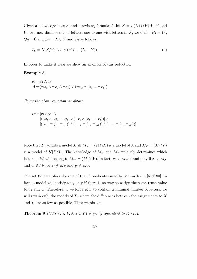
Given a knowledge base K and a revising formula A, let X = V (K) ∪ V (A), Y and
W two new distinct sets of letters, one-to-one with letters in X, we define PS = W ,
QS = ∅ and ZS = X ∪ Y and TS as follows:
TS = K[X/Y ] ∧ A ∧ (¬W ≡ (X ≡ Y )) (4)
In order to make it clear we show an example of this reduction.
Example 8
K = x1 ∧ x2
A = (¬x1 ∧ ¬x2 ∧ ¬x3) ∨ (¬x2 ∧ (x1 ≡ ¬x3))
Using the above equation we obtain
TS = [y1 ∧ y2] ∧[(¬x1 ∧ ¬x2 ∧ ¬x3) ∨ (¬x2 ∧ (x1 ≡ ¬x3))] ∧[(¬w1 ≡ (x1 ≡ y1)) ∧ (¬w2 ≡ (x2 ≡ y2)) ∧ (¬w3 ≡ (x3 ≡ y3))]
Note that TS admits a model M iff MX = (M∩X) is a model of A and MY = (M∩Y )
is a model of K[X/Y ]. The knowledge of MX and MY uniquely determines which
letters of W will belong to MW = (M ∩W ). In fact, wi ∈ MW if and only if xi ∈ MX
and yi 6∈ MY or xi 6∈ MX and yi ∈ MY .
The set W here plays the role of the ab predicates used by McCarthy in [McC80]. In
fact, a model will satisfy a wi only if there is no way to assign the same truth value
to xi and yi. Therefore, if we force MW to contain a minimal number of letters, we
will retain only the models of TS where the differences between the assignments to X
and Y are as few as possible. Thus we obtain
Theorem 9 CIRC(TS; W, ∅, X ∪ Y ) is query equivalent to K ∗S A.
20
Proof. Let γ be a formula such that V (γ) ⊆ V (K) ∪ V (A) = X. We first show that
CIRC(TS; W, ∅, X∪Y ) |= γ implies that K∗SA |= γ. Assume that CIRC(TS; W, ∅, X∪Y ) |= γ and K ∗S A 6|= γ. Thus, there exists a model MX of K ∗S A such that MX 6|= γ.
Let M ′X be a model of K such that M ′
X∆MX ∈ δ(K, A). We define MY = {yi|xi ∈M ′
X} and MW = {wi|((xi ∈ MX) and (yi 6∈ MY )) or ((xi 6∈ MX) and (yi ∈ MY ))}.Now, let M = MX ∪ MY ∪ MW . Obviously, it holds that M |= TS and M 6|= γ. If
M is a (W,X ∪ Y )-minimal model the thesis follows, so assume that there exists a
model N of TS such that N <(P,Z) M . Since N is a model of TS and it cannot contain
more literals of W than M , we have that NW = (N ∩W ) ⊂ MW . Hence, the distance
between NX = N ∩ X and NY = N ∩ Y is smaller than the distance between MX
and MY . Thus, MX is not one of the models of A closest to the models of K. As a
consequence, MX is not a model of K ∗S A and contradiction arises.
We now show that K ∗S A |= γ implies that CIRC(TS; W, ∅, X ∪ Y ) |= γ. Assume
that K ∗S A |= γ and CIRC(TS; W, ∅, X ∪ Y ) 6|= γ. Thus, there exists a model M
of CIRC(TS; W, ∅, X ∪ Y ) such that M 6|= γ. Let MX = M ∩ X, we show that
MX |= K ∗S A. It immediately follows that MX |= A, if MX is one of the models
of A closer to models of K the thesis follows, so assume to the contrary that there
exists a NX ⊆ X, different from MX , such that NX |= A and the distance of MX
from the closest model of K is a strict superset of the distance of NX from its closest
model of K, i.e. , µ(NX , K) ⊆ µ(MX , K) and µ(NX , K) 6= µ(MX , K). Let N ′X be a
model of K such that N ′X∆NX ∈ δ(K,A). Let NY = {yi|xi ∈ N ′
X}, NW = {wi|((xi ∈NX) and (yi 6∈ NY )) or ((xi 6∈ NX) and (yi ∈ NY ))} and N = NX ∪ NY ∪ NW .
Obviously N is a model of K[X/Y ] ∧ A ∧ (¬W ≡ (X ≡ Y )) moreover, N <(P,Z) M .
Hence, M is not a (W,X ∪ Y )-minimal model of K[X/Y ] ∧ A ∧ (¬W ≡ (X ≡ Y )),
hence contradiction arises.
Summing up, we have a modular poly-time reduction from CIRC into Satoh’s revision
21
that satisfies logical equivalence and a reverse (modular and poly-time) reduction
that only satisfies query equivalence. It is natural to ask whether there exists a (poly-
time or poly-size) reduction from Satoh’s revision into CIRC that preserves logical
equivalence. Using the result proven in [LS96a] on the complexity of model checking
for Satoh’s operator and the known complexity of model checking for CIRC (see
[Cad92]), we can show that:
Theorem 10 Unless Σp2 = coNP, there is no poly-time reduction from K ∗S A into
CIRC(T ; P, Q, Z) satisfying logical-equivalence. Unless Σp4 = Πp
4, there is no poly-size
reduction from K ∗S A into CIRC(T ; P, Q, Z) satisfying logical-equivalence.
Proof. In [LS96a] we have shown that the time complexity of deciding whether M |=K ∗S A is Σp
2-complete and that the compilability level of this problem is nu-comp-
Σp2-complete. In [Cad92] it is shown that deciding whether M |= CIRC(T ; P,Q, Z)
is coNP-complete and in [CDLS96a] we proved that the compilability level of this
problem is nu-comp-coNP-complete. As a consequence, if there exists a poly-time
reduction from K ∗S A into CIRC(T ; P,Q, Z) satisfying logical-equivalence we have
that a Σp2-complete can be reduced to a coNP-complete one, and thus, Σp
2 ⊆ coNP.
If there exists a poly-size reduction it follows that nu-comp-Σp2 ⊆ nu-comp-coNP(the
definition of this class is in the appendix). By [CDLS96a, Theorem 9] this implies
that Σp4 = Πp
4.
3.2 Dalal’s revision
The same reductions between Satoh’s revision and usual (set-containment-based) cir-
cumscription hold between Dalal’s revision [Dal88] and cardinality-based circumscrip-
tion. Proofs of all the following theorems are in the appendix.
22
Theorem 11 (¬P ) ∗D T is logically equivalent to NCIRC(T ; P, ∅, Z).
Note that the above reduction is modular, computable in polynomial time and satisfies
both logical and query-equivalence, but it assumes that Q = ∅. By combining the
above theorem and Corollary 5 we obtain:
Corollary 12 (¬P ) ∗D (T ∧ (Q ≡ ¬Q′)) is query equivalent to NCIRC(T ; P, Q,Z).
where Q′ is a set of new letters one-to-one with letters in Q. To reduce Dalal’s revision
into cardinality-based circumscription, we use the same relation adopted to reduce
Satoh’s revision into CIRC:
K ∗D A ⇒ NCIRC(TD; W, ∅, X ∪ Y )
where X = V (T )∪ V (A) and TD = K[X/Y ]∧A∧ (¬W ≡ (X ≡ Y )). Note that, not
surprisingly, TD coincides with TS.
Theorem 13 NCIRC(TD; W, ∅, X ∪ Y ) is query equivalent to K ∗D A.
We have shown a reduction from NCIRC into Dalal’s revision that satisfies logical
equivalence and a reverse reduction that only satisfies query equivalence. We show
that, unless there is a collapse in the polynomial hierarchy, there is no poly-size or
polytime reduction from Dalal’s revision into NCIRC that preserves logical equiva-
lence.
Theorem 14 Unless NP = coNP, there is no poly-time reduction from K ∗D A into
NCIRC(T ; P, Q, Z) satisfying logical-equivalence. Unless Σp3 = Πp
3, there is no poly-
size reduction from K ∗D A into NCIRC(T ; P,Q, Z) satisfying logical-equivalence.
We end this section with a complete example of application of our reductions. We
continue example (8) and reduce Satoh’s and Dalal’s revision to CIRC and NCIRC,
respectively.
23
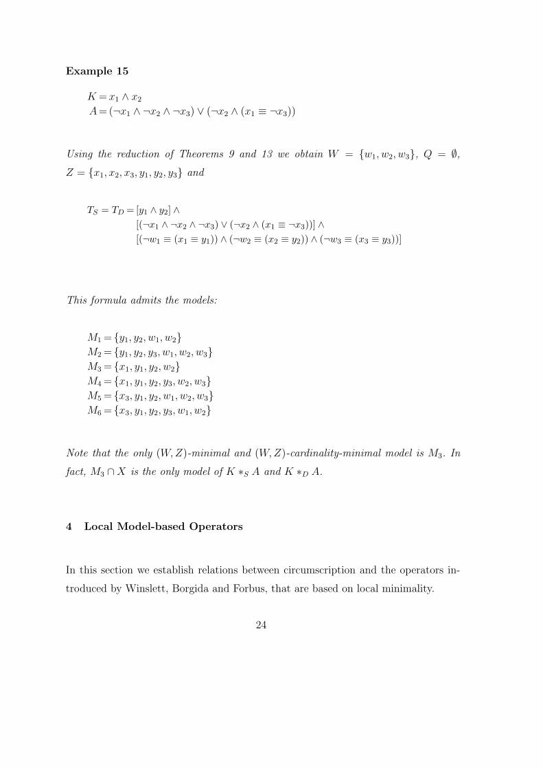
Example 15
K = x1 ∧ x2
A = (¬x1 ∧ ¬x2 ∧ ¬x3) ∨ (¬x2 ∧ (x1 ≡ ¬x3))
Using the reduction of Theorems 9 and 13 we obtain W = {w1, w2, w3}, Q = ∅,Z = {x1, x2, x3, y1, y2, y3} and
TS = TD = [y1 ∧ y2] ∧[(¬x1 ∧ ¬x2 ∧ ¬x3) ∨ (¬x2 ∧ (x1 ≡ ¬x3))] ∧[(¬w1 ≡ (x1 ≡ y1)) ∧ (¬w2 ≡ (x2 ≡ y2)) ∧ (¬w3 ≡ (x3 ≡ y3))]
This formula admits the models:
M1 = {y1, y2, w1, w2}M2 = {y1, y2, y3, w1, w2, w3}M3 = {x1, y1, y2, w2}M4 = {x1, y1, y2, y3, w2, w3}M5 = {x3, y1, y2, w1, w2, w3}M6 = {x3, y1, y2, y3, w1, w2}
Note that the only (W,Z)-minimal and (W,Z)-cardinality-minimal model is M3. In
fact, M3 ∩X is the only model of K ∗S A and K ∗D A.
4 Local Model-based Operators
In this section we establish relations between circumscription and the operators in-
troduced by Winslett, Borgida and Forbus, that are based on local minimality.
24
4.1 Winslett’s update
Winslett’s update method modifies models of K one-by-one, replacing each one with
the closest one within the models of A. Local proximity methods are better related
to circumscription where all letters are minimized. Circumscription without varying
and fixed letters (i.e. Q = Z = ∅) is immediately expressed as
CIRC(T ; P, ∅, ∅) ⇒ ¬P ∗W T
Theorem 16 (¬P ) ∗W T is logically equivalent to CIRC(T ; P, ∅, ∅).
In order to reduce Winslett’s update into circumscription, we must ensure that to each
distinct model of K correspond incomparable models in the circumscriptive theory.
Let X = V (K)∪V (A), Y and W be new sets of distinct variables, each one-to-one with
variables in X. The desired relation is obtained (only satisfying query-equivalence)
using the following equation:
TW = K[X/Y ] ∧ A ∧ (¬W ≡ (X ≡ Y )) (5)
In fact, we have
Theorem 17 CIRC(TW ; W,Y,X) is query equivalent to K ∗W A.
Note that TW is equal to TS, but now the letters in Y are kept fixed, not minimized.
We show a negative proof on the existence of a (poly-size or poly-time) reduction
from Winslett’s revision into CIRC that satisfies logical equivalence.
Theorem 18 Unless Σp2 = coNP, there is no poly-time reduction from K ∗W A into
CIRC(T ; P, Q, Z) satisfying logical-equivalence. Unless Σp4 = Πp
4, there is no poly-size
reduction from K ∗W A into CIRC(T ; P, Q,Z) satisfying logical-equivalence.
25
4.2 Borgida’s revision
Borgida’s revision operator [Bor85] is very similar to Winslett’s one, the only differ-
ence being that the result of the first one has to be K ∧ A when not contradictory.
It is easy to show that ∗B and ∗W coincide when K has a single model M . In fact,
if M is also a model of A, then K ∗W A = K ∧ A = K ∗B A. If M is not a model of
A the equivalence follows from the definition. As a consequence, the same reduction
used for ∗W also holds for ∗B. That is:
CIRC(T ; P, ∅, ∅) ⇒ ¬P ∗B T
In the other direction, one can find a direct transformation from Borgida’s revision
into circumscription, very much like Winslett’s one. The fact that the result must be
K ∧A can be taken into account by selecting the models of this formula as minimal.
K ∗B A ⇒ CIRC(TB; R ∪ Z ∪W, ∅, X ∪ Y )
where X = V (K) ∪ V (A), Y , W and R are new sets one-to-one with the elements of
X and TB is defined as follows:
TB = [K ∨ (Y ≡ R)] ∧K[X/Y ] ∧ A ∧ [¬W ≡ (X ≡ Y )] (6)
In fact, we have
Theorem 19 CIRC(TB; W,R, X ∪ Y ) is query equivalent to K ∗B A.
As for the other operators, we show a negative proof on the existence of a (poly-
size or poly-time) reduction from Winslett’s revision into CIRC that satisfies logical
equivalence.
26
Theorem 20 Unless Σp2 = coNP, there is no poly-time reduction from K ∗B A into
CIRC(T ; P, Q, Z) satisfying logical-equivalence. Unless Σp4 = Πp
4, there is no poly-size
reduction from K ∗B A into CIRC(T ; P,Q, Z) satisfying logical-equivalence.
4.3 Forbus’ update
We first observe how circumscription and NCIRC can be expressed using Forbus’
update. Reduction of NCIRC to Forbus’ operator is trivial:
NCIRC(T ; P, ∅, ∅) ⇒ ¬P ∗F T
Theorem 21 (¬P ) ∗F T is logically equivalent to NCIRC(T ; P, ∅, ∅).
The reduction of Forbus’ update to circumscription is very similar to Borgida’s one.
We have only to take in account that Forbus’ update is based upon a minimization
of the cardinality of the distances between models.
The reduction is:
K ∗F A ⇒ CIRC(TF ; V, Y,X ∪W )
where TF is defined as:
TF = K[X/Y ] ∧ A ∧ (¬W ≡ (X ≡ Y )) ∧ EQ(W,V ) ∧BEGIN(V ) (7)
The formula EQ(W,V ) is a polynomial-size formula that is true if and only if W and
V have exactly the same number of positive literals. It can be costructed in several
ways, if n is the cardinality of the two sets, the simpler formula representing this
boolean function uses two n-bits adders and then forces the two results to become
(bit-by-bit) equal. Finally, BEGIN(V ) states that the positive literals of V are its
27
first ones:
BEGIN(V ) = (vn → vn−1) ∧ . . . ∧ (v2 → v1)
Any interpreation M of V ∪ W satisfying EQ(W,V ) ∧ BEGIN(V ) is such that
|M ∩ V | = |M ∩W | and vi ∈ M if and only if for all 1 ≤ j < i we have vi ∈ M . That
is, an intepretation of the set V has all the true atoms “at the beginning”.
In fact, we have
Theorem 22 CIRC(TF ; V, Y, X ∪W ) is query equivalent to K ∗F A.
Summing up, we have a reduction from NCIRC into Forbus’ revision that satisfies
logical equivalence (when Q = Z = ∅) and a reduction from ∗F to CIRC that only
satisfies query equivalence. We show a negative proof on the existence of a reduction
from Forbus’ revision into CIRC that satisfies logical equivalence.
Theorem 23 Unless Σp2 = coNP, there is no poly-time reduction from K ∗F A into
CIRC(T ; P, Q, Z) satisfying logical-equivalence. Unless Σp4 = Πp
4, there is no poly-size
reduction from K ∗F A into CIRC(T ; P, Q,Z) satisfying logical-equivalence.
We end this section with an example of application of our reductions. We reduce
Winslett, Borgida and Forbus’ operators to CIRC.
Example 24 We use the same formulae K and A used in Example 8.
K = x1 ∧ x2
A = (¬x1 ∧ ¬x2 ∧ ¬x3) ∨ (¬x2 ∧ (x1 ≡ ¬x3))
For Winslett’s revision we use the reduction of Theorem 17 and we obtain P =
{w1, w2, w3}, Q = {y1, y2, y3}, Z = {x1, x2, x3} and TW
28
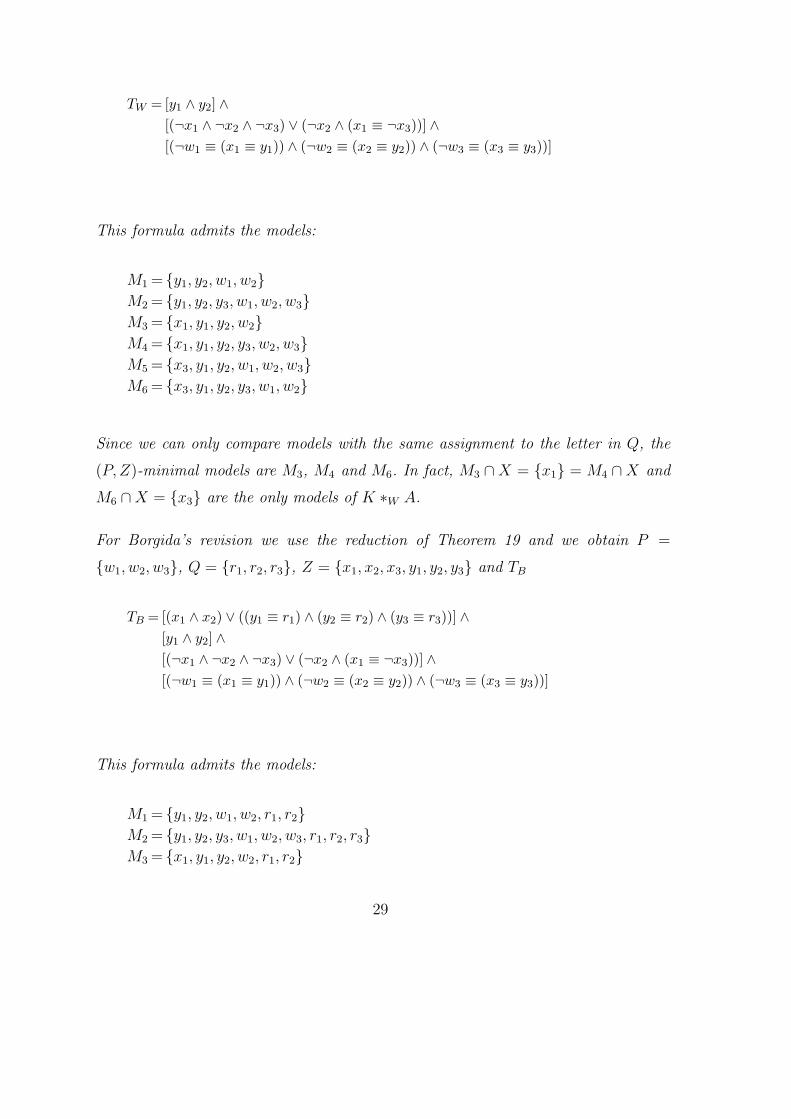
TW = [y1 ∧ y2] ∧[(¬x1 ∧ ¬x2 ∧ ¬x3) ∨ (¬x2 ∧ (x1 ≡ ¬x3))] ∧[(¬w1 ≡ (x1 ≡ y1)) ∧ (¬w2 ≡ (x2 ≡ y2)) ∧ (¬w3 ≡ (x3 ≡ y3))]
This formula admits the models:
M1 = {y1, y2, w1, w2}M2 = {y1, y2, y3, w1, w2, w3}M3 = {x1, y1, y2, w2}M4 = {x1, y1, y2, y3, w2, w3}M5 = {x3, y1, y2, w1, w2, w3}M6 = {x3, y1, y2, y3, w1, w2}
Since we can only compare models with the same assignment to the letter in Q, the
(P,Z)-minimal models are M3, M4 and M6. In fact, M3 ∩X = {x1} = M4 ∩X and
M6 ∩X = {x3} are the only models of K ∗W A.
For Borgida’s revision we use the reduction of Theorem 19 and we obtain P =
{w1, w2, w3}, Q = {r1, r2, r3}, Z = {x1, x2, x3, y1, y2, y3} and TB
TB = [(x1 ∧ x2) ∨ ((y1 ≡ r1) ∧ (y2 ≡ r2) ∧ (y3 ≡ r3))] ∧[y1 ∧ y2] ∧[(¬x1 ∧ ¬x2 ∧ ¬x3) ∨ (¬x2 ∧ (x1 ≡ ¬x3))] ∧[(¬w1 ≡ (x1 ≡ y1)) ∧ (¬w2 ≡ (x2 ≡ y2)) ∧ (¬w3 ≡ (x3 ≡ y3))]
This formula admits the models:
M1 = {y1, y2, w1, w2, r1, r2}M2 = {y1, y2, y3, w1, w2, w3, r1, r2, r3}M3 = {x1, y1, y2, w2, r1, r2}
29
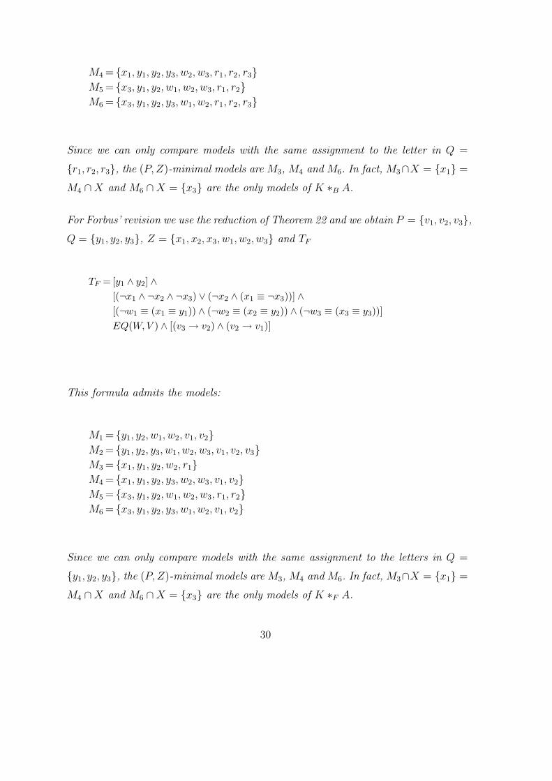
M4 = {x1, y1, y2, y3, w2, w3, r1, r2, r3}M5 = {x3, y1, y2, w1, w2, w3, r1, r2}M6 = {x3, y1, y2, y3, w1, w2, r1, r2, r3}
Since we can only compare models with the same assignment to the letter in Q =
{r1, r2, r3}, the (P,Z)-minimal models are M3, M4 and M6. In fact, M3∩X = {x1} =
M4 ∩X and M6 ∩X = {x3} are the only models of K ∗B A.
For Forbus’ revision we use the reduction of Theorem 22 and we obtain P = {v1, v2, v3},Q = {y1, y2, y3}, Z = {x1, x2, x3, w1, w2, w3} and TF
TF = [y1 ∧ y2] ∧[(¬x1 ∧ ¬x2 ∧ ¬x3) ∨ (¬x2 ∧ (x1 ≡ ¬x3))] ∧[(¬w1 ≡ (x1 ≡ y1)) ∧ (¬w2 ≡ (x2 ≡ y2)) ∧ (¬w3 ≡ (x3 ≡ y3))]EQ(W,V ) ∧ [(v3 → v2) ∧ (v2 → v1)]
This formula admits the models:
M1 = {y1, y2, w1, w2, v1, v2}M2 = {y1, y2, y3, w1, w2, w3, v1, v2, v3}M3 = {x1, y1, y2, w2, r1}M4 = {x1, y1, y2, y3, w2, w3, v1, v2}M5 = {x3, y1, y2, w1, w2, w3, r1, r2}M6 = {x3, y1, y2, y3, w1, w2, v1, v2}
Since we can only compare models with the same assignment to the letters in Q =
{y1, y2, y3}, the (P, Z)-minimal models are M3, M4 and M6. In fact, M3∩X = {x1} =
M4 ∩X and M6 ∩X = {x3} are the only models of K ∗F A.
30

5 Formula-based Operators
The only formula-based operator we have analyzed is SBR, introduced by Ginsberg
and Fagin, Ullman and Vardi. This operator is quite similar to Satoh’s principle of
minimization. The main difference between them is that the latter minimizes distance
given as set of literals, while the first one maximizes the number of preserved formulae
of K.
Two simple reductions from SBR into circumscription, and viceversa, are the following
ones:
CIRC(T ; P, ∅, Z)⇒ (¬P ) ∗SBR T
K ∗SBR A⇒CIRC(TSBR; Y, ∅, X)
where K = {f1 . . . , fm}, X = V (K) ∪ V (A), Y is a set of m new letters one-to-one
with formulae of K and TSBR is defined as
TSBR = A ∧ (y1 ≡ ¬f1) ∧ · · · ∧ (ym ≡ ¬fm)
More precisely, we have:
Theorem 25 (¬P )∗SBRT is logically equivalent to CIRC(T ; P, ∅, Z) and CIRC(TSBR; Y, ∅, X)
is query equivalent to K ∗SBR A.
Using Corollary 4 we can also obtain a reduction from CIRC(T ; P,Q, Z) into SBR
that preserves query equivalence. We close this section with an example of application
of our reductions. We reduce SBR to CIRC.
Example 26 We use the same formulae K and A used in Example 8, but K is now
a set of two formulae.
31
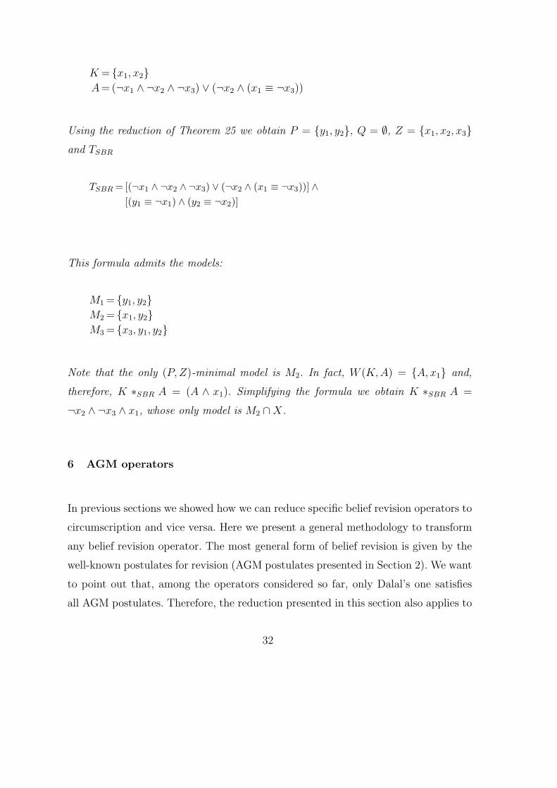
K = {x1, x2}A = (¬x1 ∧ ¬x2 ∧ ¬x3) ∨ (¬x2 ∧ (x1 ≡ ¬x3))
Using the reduction of Theorem 25 we obtain P = {y1, y2}, Q = ∅, Z = {x1, x2, x3}and TSBR
TSBR = [(¬x1 ∧ ¬x2 ∧ ¬x3) ∨ (¬x2 ∧ (x1 ≡ ¬x3))] ∧[(y1 ≡ ¬x1) ∧ (y2 ≡ ¬x2)]
This formula admits the models:
M1 = {y1, y2}M2 = {x1, y2}M3 = {x3, y1, y2}
Note that the only (P, Z)-minimal model is M2. In fact, W (K, A) = {A, x1} and,
therefore, K ∗SBR A = (A ∧ x1). Simplifying the formula we obtain K ∗SBR A =
¬x2 ∧ ¬x3 ∧ x1, whose only model is M2 ∩X.
6 AGM operators
In previous sections we showed how we can reduce specific belief revision operators to
circumscription and vice versa. Here we present a general methodology to transform
any belief revision operator. The most general form of belief revision is given by the
well-known postulates for revision (AGM postulates presented in Section 2). We want
to point out that, among the operators considered so far, only Dalal’s one satisfies
all AGM postulates. Therefore, the reduction presented in this section also applies to
32
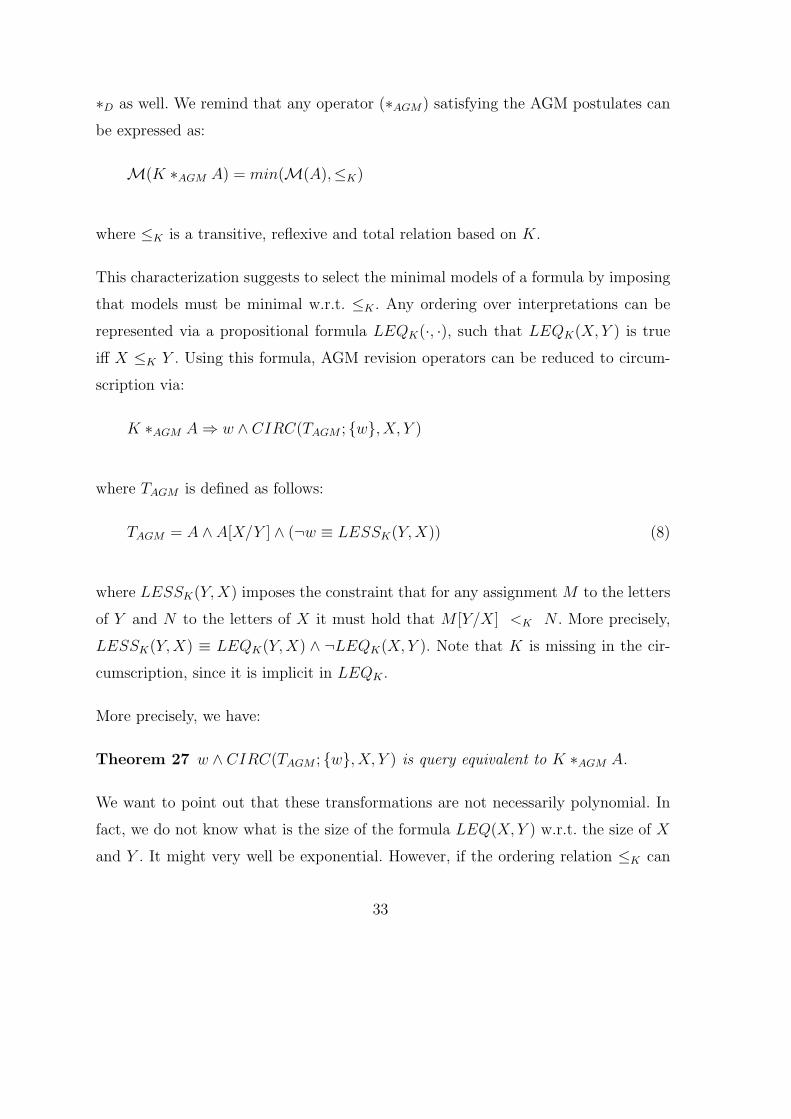
∗D as well. We remind that any operator (∗AGM) satisfying the AGM postulates can
be expressed as:
M(K ∗AGM A) = min(M(A),≤K)
where ≤K is a transitive, reflexive and total relation based on K.
This characterization suggests to select the minimal models of a formula by imposing
that models must be minimal w.r.t. ≤K . Any ordering over interpretations can be
represented via a propositional formula LEQK(·, ·), such that LEQK(X, Y ) is true
iff X ≤K Y . Using this formula, AGM revision operators can be reduced to circum-
scription via:
K ∗AGM A ⇒ w ∧ CIRC(TAGM ; {w}, X, Y )
where TAGM is defined as follows:
TAGM = A ∧ A[X/Y ] ∧ (¬w ≡ LESSK(Y,X)) (8)
where LESSK(Y, X) imposes the constraint that for any assignment M to the letters
of Y and N to the letters of X it must hold that M [Y/X] <K N . More precisely,
LESSK(Y,X) ≡ LEQK(Y,X) ∧ ¬LEQK(X, Y ). Note that K is missing in the cir-
cumscription, since it is implicit in LEQK .
More precisely, we have:
Theorem 27 w ∧ CIRC(TAGM ; {w}, X, Y ) is query equivalent to K ∗AGM A.
We want to point out that these transformations are not necessarily polynomial. In
fact, we do not know what is the size of the formula LEQ(X,Y ) w.r.t. the size of X
and Y . It might very well be exponential. However, if the ordering relation ≤K can
33
be decided in polynomial time, then the formula LEQK(X,Y ) has size polynomial.
7 Relations among belief revision operators
In Sections 3, 4, 5 and 6 we found relations between circumscription and belief revision
operators. Here we focus on relations among the various revision operators.
In particular, we show that Satoh’s and Ginsberg, Fagin, Ullman and Vardi’s oper-
ators can be reduced one to the other and that Winslett’s one can be reduced to
both. Note that these operators belong to three different classes of operators, namely
formula-based (Ginsberg, Fagin, Ullman and Vardi), model-based with global prox-
imity (Satoh) and model-based with local proximity (Winslett). Therefore, our results
make evident the similarities between all these operators, pointing out, at the same
time, their differences.
Ginsberg, Fagin, Ullman and Vardi’s operator can be reduced to Satoh’s operator via:
K ∗SBR A ⇒ Y ∗S A′
where K = {f1 . . . , fm}, Y is a set of m new letters one-to-one with formulae of K
and
A′ = A ∧ (y1 → f1) ∧ · · · ∧ (ym → fm)
More formally we have:
Theorem 28 Y ∗S A′ is query equivalent to K ∗SBR A.
The reverse reduction is:
K ∗S A ⇒ W ∗SBR A′′
34
where Y and W are sets of new letters one to one with letters of X and
A′′ = K[X/Y ] ∧ A ∧ (W → (X ≡ Y ))
More formally we have:
Theorem 29 W ∗SBR A′′ is query equivalent to K ∗S A.
More complex, but still computable in polynomial time, is the reduction of Winslett’s
operator into SBR. Denoting with F the following formula:
F = K[X/Y ] ∧ A ∧ (¬Y ∨ ¬Z) ∧ (W → (X ≡ Y ))
where Y , W and Z are sets of new letters one to one with letters of X. The reduction
is now the following one:
K ∗W A ⇒ (W ∪ Y ∪ Z) ∗SBR F
More formally we have:
Theorem 30 (W ∪ Y ∪ Z) ∗SBR F is query equivalent to K ∗W A.
Composing the reductions of ∗W to ∗SBR and ∗SBR to ∗S we have a reduction of ∗W to
∗S. All these reductions only preserve query equivalence, we show that there cannot
be any (poly-size or poly-time) reduction from either Winslett’s or Satoh’s operatot
into SBR.
Theorem 31 Unless Σp2 = coNP, there is no poly-time reduction from K ∗S A (K ∗W
A) into K ′∗SBRA′ satisfying logical-equivalence. Unless Σp4 = Πp
4, there is no poly-size
reduction from K ∗S A (K ∗W A) into K ′ ∗SBR A′ satisfying logical-equivalence.
35
8 Syntactically-restricted Knowledge Bases
In this section we focus on knowledge bases of a restricted syntactic form. Among the
restricted cases, Horn knowledge bases are of particular interest for several reasons.
First of all, since Horn clauses can represent if-then relations, they are expressive
enough to represent many real situations. Moreover, reasoning with Horn knowledge
bases is significantly simpler than reasoning with general ones (see [DG84]) and also
revising them is, in general, simpler than revising general ones (see [EG92]).
While reductions from circumscription to belief revision preserve the syntactic form of
the original theory, reductions from belief revision to circumscription do not preserve
the syntactic form of the formulae. As an example, notice that the relation X ≡ ¬Y
cannot be expressed as an Horn formula.
As a consequence, it is easy to apply results on restricted cases of belief revision to
circumscription, but the other way around is less likely to produce interesting results.
There are several reasons why the revision of Horn theories cannot be expressed as the
circumscription of a Horn formula. First of all, results of Eiter and Gottlob show that
reasoning with the revision of a Horn knowledge base is coNP-hard for all operators
considered, while reasoning with Horn theories under circumscription is a polynomial
task. As a consequence, reductions from belief revision to circumscription preserving
the syntactic form cannot be done in polynomial time (assuming P 6= NP).
Secondly, the result of revising a Horn knowledge base with a Horn formula might
be a non-Horn formula. For example, the result of {a, b} ∗ (¬a ∨ ¬b) is a ≡ ¬b for all
operators, and a ≡ ¬b cannot be expressed as an Horn formula. On the other hand,
the circumscription of a Horn theory is an Horn theory.
36
9 Analysis and Discussion
In the previous sections we showed new relations relating belief revision operators
and circumscription. These relations point out the close connections between the two
fields. We want to point out that our relations can be easily extended to full first-
order languages, whenever the belief revision operators are defined in this setting.
Take, for example, the reduction from circumscription into Satoh’s revision operator.
The reduction also applies when K and A are arbitrary first-order sentences. Clearly,
in this case X is a set of n predicates, each one with its arity, while W and Y are new
sets of n predicates, one-to-one with the predicates of X. Moreover, the constraint
¬W ≡ (X ≡ Y ) must be expressed as:
n∧
i=1
∀zk(¬wi(zk) ≡ (xi(z
k) ≡ yi(zk)))
where wi, xi and yi are k-ary predicates and zk is a vector of k variables.
Many side benefits can be obtained from the established relations. In this section we
want to point out the most important benefits obtained.
9.1 Compact Representation of NCIRC
In two recent papers [CDSS95,CDLS95] Cadoli, Donini and the present authors an-
alyze the size of the explicit representation of circumscription and belief revision
operators. More precisely, taking as an example belief revision, it is determined the
size of the smallest propositional formula K1 that is equivalent to K ∗ A, where ∗ is
one of the belief revision operators analyzed.
As it turns out, the size of the explicit representation of the result of revising a
knowledge base is, in general, exponential w.r.t. |K|+ |A|. Differences arise between
37
the various operators. The result of revising a knowledge base using Dalal’s revision
operator admits a polynomial-sized explicit representation, if we allow new variables
in the representation. More precisely, there exists a formula K1 using the letters of
K and A and possibly new ones, whose size is polynomial in |K|+ |A|, s.t. , for any
q using only variables of K and A we have that K1 |= q if and only if K ∗D A |= q.
We show that NCIRC(T ; P,Q, Z) always admits an explicit representation whose
size is polynomial w.r.t. |T |, via the proof given for Dalal’s belief revision operator.
NCIRC(T ; P, Q, Z) is the set of models of T with a least number of elements. Given
T and P , we first compute the least number k of true letters of the set P in the models
of T . At this point, we constrain the formula to have only models that contain atmost
k letters of the set P . This forces the formula to only retain the (P, Z)-cardinality-
minimal models of T . This can be accomplished by conjoining T with a formula
imposing that at most k letters of the set P must be true. That is:
NCIRC(T ; P, Q,Z) = T ∧ATMOST (k, P )
The formula ATMOST (k, P ) can be constructed using an n-bit adder (where n =
|P |) for the letters of P and then constraining the result to coincide with the bi-
nary representation of k. This a formula has size O(n3). Thus, the size of T ∧ATMOST (k, P ) is polynomial in |T |.
9.2 Computational Complexity Analysis
A valuable byproduct of the reductions presented in this work is the ability of im-
porting complexity results obtained in one field into the other one. For example, in
the general case, inference using the belief revision operators introduced by Satoh,
Borgida and Winslett has the same complexity of inference under circumscription.
While this result is not novel, it has been proven in [EG93,EG92], several other inter-
38
esting results can be obtained. As an example, it is known that deciding whether a
clause follows from the circumscription (with all letters minimized) of a theory com-
posed of binary clauses (i.e. clauses with at most two literals) is a coNP-hard problem
[CL94]. We can use this result to prove that inference in the revision of a knowledge
base composed of binary clauses is a coNP-hard problem for most operators.
Corollary 32 Let K and A be two CNF formula where all clauses have at most two
literals, and Q be a clause. The problem of deciding whether K ∗A |= Q is coNP-hard
for ∗ ∈ {∗S, ∗D, ∗W , ∗B, ∗SBR}.
10 Conclusions
We have presented a complete analysis of the relations between belief revision op-
erators on one hand and circumscription and its cardinality-based variant on the
other hand. Furthermore, we have pointed out the many benefits that the established
correlations can deliver to the analysis of both fields.
Our results greatly extends Winslett’s results on transforming her revision operator
into circumscription presented in [Win89]. Even though Winslett’s analysis could be
further extended to deal with other operators, our results provide us with more direct
and simple translations.
Acknowledgments
We want to thank Marco Cadoli for helpful discussions on the content of this paper.
39
References
[AGfM85] C. E. Alchourron, P. Gardenfors, and D. Makinson. On the logic of theory
change: Partial meet contraction and revision functions. Journal of Symbolic
Logic, 50:510–530, 1985.
[Bor85] A. Borgida. Language features for flexible handling of exceptions in information
systems. ACM Transactions on Database Systems, 10:563–603, 1985.
[Cad92] M. Cadoli. The complexity of model checking for circumscriptive formulae.
Information Processing Letters, 44:113–118, 1992.
[CDLS95] M. Cadoli, F. M. Donini, P. Liberatore, and M. Schaerf. The size of a revised
knowledge base. In Proceedings of the Fourteenth ACM SIGACT SIGMOD
SIGART Symposium on Principles of Database Systems (PODS-95), pages 151–
162, 1995.
[CDLS96a] M. Cadoli, F. M. Donini, P. Liberatore, and M. Schaerf. Feasibility and
unfeasibility of off-line processing. In Proceedings of the Fourth Israeli
Symposium on Theory of Computing and Systems (ISTCS-96), pages 100–109,
1996.
[CDLS96b] Marco Cadoli, Francesco M. Donini, Paolo Liberatore, and Marco Schaerf.
Comparing space efficiency of propositional knowledge representation
formalisms. In Proceedings of the Fifth International Conference on the
Principles of Knowledge Representation and Reasoning (KR-96), 1996. To
Appear.
[CDSS95] M. Cadoli, F. M. Donini, M. Schaerf, and R. Silvestri. On compact
representations of propositional circumscription. Technical Report RAP.14.95,
Dipartimento di Informatica e Sistemistica, Universita di Roma “La Sapienza”,
July 1995. To appear in Theoretical Computer Science. Short version appeared
in Proceedings of the Twelfth Symposium on Theoretical Aspects of Computer
Science (STACS-95), pages 205–216.
40
[CEG92] M. Cadoli, T. Eiter, and G. Gottlob. An efficient method for eliminating varying
predicates from a circumscription. Artificial Intelligence Journal, 54:397–410,
1992.
[CL94] M. Cadoli and M. Lenzerini. The complexity of propositional closed world
reasoning and circumscription. Journal of Computer and System Sciences,
48:255–310, 1994.
[Dal88] M. Dalal. Investigations into a theory of knowledge base revision: Preliminary
report. In Proceedings of the Seventh National Conference on Artificial
Intelligence (AAAI-88), pages 475–479, 1988.
[DG84] W. P. Dowling and J. H. Gallier. Linear-time algorithms for testing the
satisfiability of propositional Horn formulae. Journal of Logic Programming,
1:267–284, 1984.
[dKK89] J. de Kleer and K. Konolige. Eliminating the fixed predicates from a
circumscription. Artificial Intelligence Journal, 39:391–398, 1989.
[EG92] T. Eiter and G. Gottlob. On the complexity of propositional knowledge base
revision, updates and counterfactuals. Artificial Intelligence Journal, 57:227–
270, 1992.
[EG93] T. Eiter and G. Gottlob. Propositional circumscription and extended closed
world reasoning are Πp2-complete. Theoretical Computer Science, 114:231–245,
1993.
[For89] K. D. Forbus. Introducing actions into qualitative simulation. In Proceedings of
the Eleventh International Joint Conference on Artificial Intelligence (IJCAI-
89), pages 1273–1278, 1989.
[FUV83] R. Fagin, J. D. Ullman, and M. Y. Vardi. On the semantics of updates in
databases. In Proceedings of the Second ACM SIGACT SIGMOD Symposium
on Principles of Database Systems (PODS-83), pages 352–365, 1983.
41
[Gar88] P. Gardenfors. Knowledge in Flux: Modeling the Dynamics of Epistemic States.
Bradford Books, MIT Press, Cambridge, MA, 1988.
[Gin86] M. L. Ginsberg. Conterfactuals. Artificial Intelligence Journal, 30:35–79, 1986.
[Gin89] M. L. Ginsberg. A circumscriptive theorem prover. Artificial Intelligence
Journal, 39:209–230, 1989.
[GJ79] M. R. Garey and D. S. Johnson. Computers and Intractability, A Guide to the
Theory of NP-Completeness. W.H. Freeman and Company, San Francisco, Ca,
1979.
[Imi87] T. Imielinski. Results on translating defaults to circumscription. Artificial
Intelligence Journal, 32:131–146, 1987.
[Joh90] D. S. Johnson. A catalog of complexity classes. In J. van Leeuwen, editor,
Handbook of Theoretical Computer Science, volume A, chapter 2. Elsevier
Science Publishers (North-Holland), Amsterdam, 1990.
[KM89] H. Katsuno and A. O. Mendelzon. A unified view of propositional knowledge
base updates. In Proceedings of the Eleventh International Joint Conference on
Artificial Intelligence (IJCAI-89), pages 1413–1419, 1989.
[KM91a] H. Katsuno and A. O. Mendelzon. On the difference between updating a
knowledge base and revising it. In Proceedings of the Second International
Conference on the Principles of Knowledge Representation and Reasoning (KR-
91), pages 387–394, 1991.
[KM91b] H. Katsuno and A. O. Mendelzon. Propositional knowledge base revision and
minimal change. Artificial Intelligence Journal, 52:263–294, 1991.
[Lif85] V. Lifschitz. Computing circumscription. In Proceedings of the Ninth
International Joint Conference on Artificial Intelligence (IJCAI-85), pages 121–
127, 1985.
42
[LS95] P. Liberatore and M. Schaerf. Relating belief revision and circumscription.
In Proceedings of the Fourteenth International Joint Conference on Artificial
Intelligence (IJCAI-95), pages 1557–1563, 1995.
[LS96a] P. Liberatore and M. Schaerf. Belief revision and update: Complexity of model
checking and their relative compactness. Extended version of [LS96b], 1996.
[LS96b] P. Liberatore and M. Schaerf. The complexity of model checking for belief
revision and update. In Proceedings of the Thirteenth National Conference on
Artificial Intelligence (AAAI-96), pages 556–561, 1996.
[McC80] J. McCarthy. Circumscription - A form of non-monotonic reasoning. Artificial
Intelligence Journal, 13:27–39, 1980.
[NNS95] A. Nerode, R. T. Ng, and V. S. Subrahmanian. Computing circumscriptive
databases. I: Theory and algorithms. Information and Computation, 116:58–80,
1995.
[Prz89] T. Przymusinski. An algorithm to compute circumscription. Artificial
Intelligence Journal, 38:49–73, 1989.
[Rei80] R. Reiter. A logic for default reasoning. Artificial Intelligence Journal, 13:81–
132, 1980.
[Sat88] K. Satoh. Nonmonotonic reasoning by minimal belief revision. In Proceedings
of the International Conference on Fifth Generation Computer Systems (FGCS-
88), pages 455–462, 1988.
[Win89] M. Winslett. Sometimes updates are circumscription. In Proceedings of the
Eleventh International Joint Conference on Artificial Intelligence (IJCAI-89),
pages 859–863, 1989.
[Win90] M. Winslett. Updating Logical Databases. Cambridge University Press, 1990.
43
A Compilability Classes
In this section we summarize some definitions and results proposed in [CDLS96a]
adapting them to the context and terminology of belief revision formalisms. In that
paper we introduced a new complexity measure for decision problems, called compil-
ability. Following the intuition that a knowledge base is known well before questions
are posed to it, we divide a reasoning problem into two parts: one part is fixed or
accessible off-line (the revised knowledge base), and the second one is variable, or ac-
cessible on-line (the model). Compilability aims at capturing the on-line complexity
of solving a problem composed of such inputs, i.e., complexity wrt the second input
when the first one can be preprocessed in an arbitrary way. We introduce a new hier-
archy of classes, the non-uniform compilability classes, denoted as nu-comp-C, where
C is a generic uniform complexity class, such as NP, coNP, Σp2, . . .
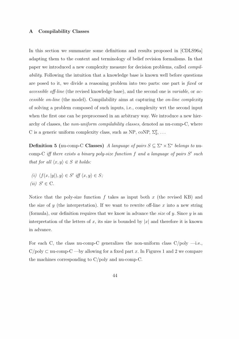
Definition 5 (nu-comp-C Classes) A language of pairs S ⊆ Σ∗×Σ∗ belongs to nu-
comp-C iff there exists a binary poly-size function f and a language of pairs S ′ such
that for all 〈x, y〉 ∈ S it holds:
(i) 〈f(x, |y|), y〉 ∈ S ′ iff 〈x, y〉 ∈ S;
(ii) S ′ ∈ C.
Notice that the poly-size function f takes as input both x (the revised KB) and
the size of y (the interpretation). If we want to rewrite off-line x into a new string
(formula), our definition requires that we know in advance the size of y. Since y is an
interpretation of the letters of x, its size is bounded by |x| and therefore it is known
in advance.
For each C, the class nu-comp-C generalizes the non-uniform class C/poly —i.e.,
C/poly ⊂ nu-comp-C —by allowing for a fixed part x. In Figures 1 and 2 we compare
the machines corresponding to C/poly and nu-comp-C.
44
|y|!!!1| |y -
y ∈ SS ′
f-
-
6
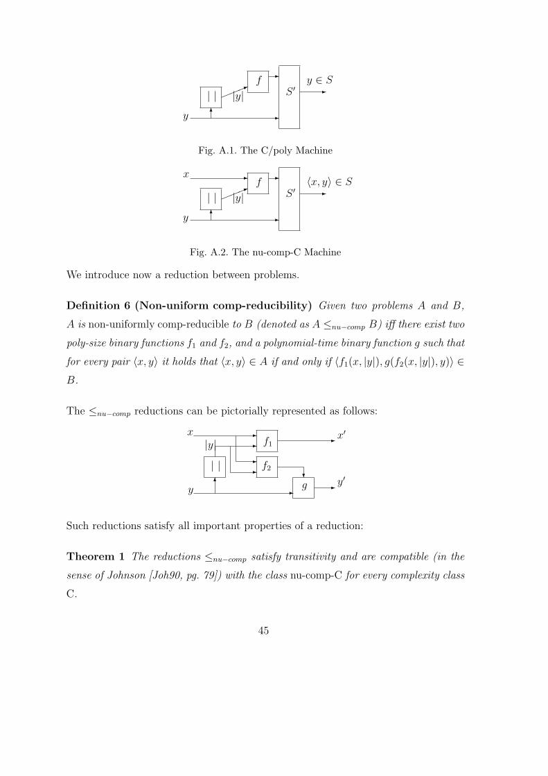
Fig. A.1. The C/poly Machine
|y|!!!1
-
| |y -
〈x, y〉 ∈ Sx
S ′f
-
-
6
Fig. A.2. The nu-comp-C Machine
We introduce now a reduction between problems.
Definition 6 (Non-uniform comp-reducibility) Given two problems A and B,
A is non-uniformly comp-reducible to B (denoted as A ≤nu−comp B) iff there exist two
poly-size binary functions f1 and f2, and a polynomial-time binary function g such that
for every pair 〈x, y〉 it holds that 〈x, y〉 ∈ A if and only if 〈f1(x, |y|), g(f2(x, |y|), y)〉 ∈B.
The ≤nu−comp reductions can be pictorially represented as follows:
|y|
-
-
6
| |y′
?
-f2
y -
x′x
g
f1-
-
-
Such reductions satisfy all important properties of a reduction:
Theorem 1 The reductions ≤nu−comp satisfy transitivity and are compatible (in the
sense of Johnson [Joh90, pg. 79]) with the class nu-comp-C for every complexity class
C.
45
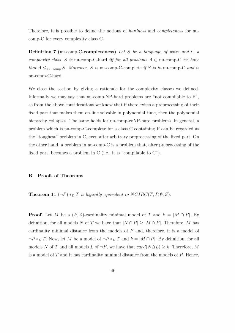
Therefore, it is possible to define the notions of hardness and completeness for nu-
comp-C for every complexity class C.
Definition 7 (nu-comp-C-completeness) Let S be a language of pairs and C a
complexity class. S is nu-comp-C-hard iff for all problems A ∈ nu-comp-C we have
that A ≤nu−comp S. Moreover, S is nu-comp-C-complete if S is in nu-comp-C and is
nu-comp-C-hard.
We close the section by giving a rationale for the complexity classes we defined.
Informally we may say that nu-comp-NP-hard problems are “not compilable to P”,
as from the above considerations we know that if there exists a preprocessing of their
fixed part that makes them on-line solvable in polynomial time, then the polynomial
hierarchy collapses. The same holds for nu-comp-coNP-hard problems. In general, a
problem which is nu-comp-C-complete for a class C containing P can be regarded as
the “toughest” problem in C, even after arbitrary preprocessing of the fixed part. On
the other hand, a problem in nu-comp-C is a problem that, after preprocessing of the
fixed part, becomes a problem in C (i.e., it is “compilable to C”).
B Proofs of Theorems
Theorem 11 (¬P ) ∗D T is logically equivalent to NCIRC(T ; P, ∅, Z).
Proof. Let M be a (P, Z)-cardinality minimal model of T and k = |M ∩ P |. By
definition, for all models N of T we have that |N ∩ P | ≥ |M ∩ P |. Therefore, M has
cardinality minimal distance from the models of P and, therefore, it is a model of
¬P ∗D T . Now, let M be a model of ¬P ∗D T and k = |M ∩ P |. By definition, for all
models N of T and all models L of ¬P , we have that card(N∆L) ≥ k. Therefore, M
is a model of T and it has cardinality minimal distance from the models of P . Hence,
46
it is a model of NCIRC(T ; P, ∅, Z).
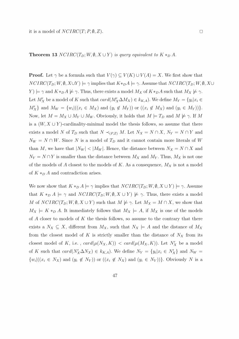
Theorem 13 NCIRC(TD; W, ∅, X ∪ Y ) is query equivalent to K ∗D A.
Proof. Let γ be a formula such that V (γ) ⊆ V (K) ∪ V (A) = X. We first show that
NCIRC(TD; W, ∅, X∪Y ) |= γ implies that K∗DA |= γ. Assume that NCIRC(TD; W, ∅, X∪Y ) |= γ and K∗DA 6|= γ. Thus, there exists a model MX of K∗DA such that MX 6|= γ.
Let M ′X be a model of K such that card(M ′
X∆MX) ∈ kK,A). We define MY = {yi|xi ∈M ′
X} and MW = {wi|((xi ∈ MX) and (yi 6∈ MY )) or ((xi 6∈ MX) and (yi ∈ MY ))}.Now, let M = MX ∪MY ∪MW . Obviously, it holds that M |= TD and M 6|= γ. If M
is a (W,X ∪ Y )-cardinality-minimal model the thesis follows, so assume that there
exists a model N of TD such that N ≺(P,Z) M . Let NX = N ∩X, NY = N ∩ Y and
NW = N ∩ W . Since N is a model of TD and it cannot contain more literals of W
than M , we have that |NW | < |MW |. Hence, the distance between NX = N ∩X and
NY = N ∩Y is smaller than the distance between MX and MY . Thus, MX is not one
of the models of A closest to the models of K. As a consequence, MX is not a model
of K ∗D A and contradiction arises.
We now show that K ∗D A |= γ implies that NCIRC(TD; W, ∅, X ∪ Y ) |= γ. Assume
that K ∗D A |= γ and NCIRC(TD; W, ∅, X ∪ Y ) 6|= γ. Thus, there exists a model
M of NCIRC(TD; W, ∅, X ∪ Y ) such that M 6|= γ. Let MX = M ∩X, we show that
MX |= K ∗D A. It immediately follows that MX |= A, if MX is one of the models
of A closer to models of K the thesis follows, so assume to the contrary that there
exists a NX ⊆ X, different from MX , such that NX |= A and the distance of MX
from the closest model of K is strictly smaller than the distance of NX from its
closest model of K, i.e. , card(µ(NX , K)) < card(µ(MX , K)). Let N ′X be a model
of K such that card(N ′X∆NX) ∈ kK,A). We define NY = {yi|xi ∈ N ′
X} and NW =
{wi|((xi ∈ NX) and (yi 6∈ NY )) or ((xi 6∈ NX) and (yi ∈ NY ))}. Obviously N is a
47
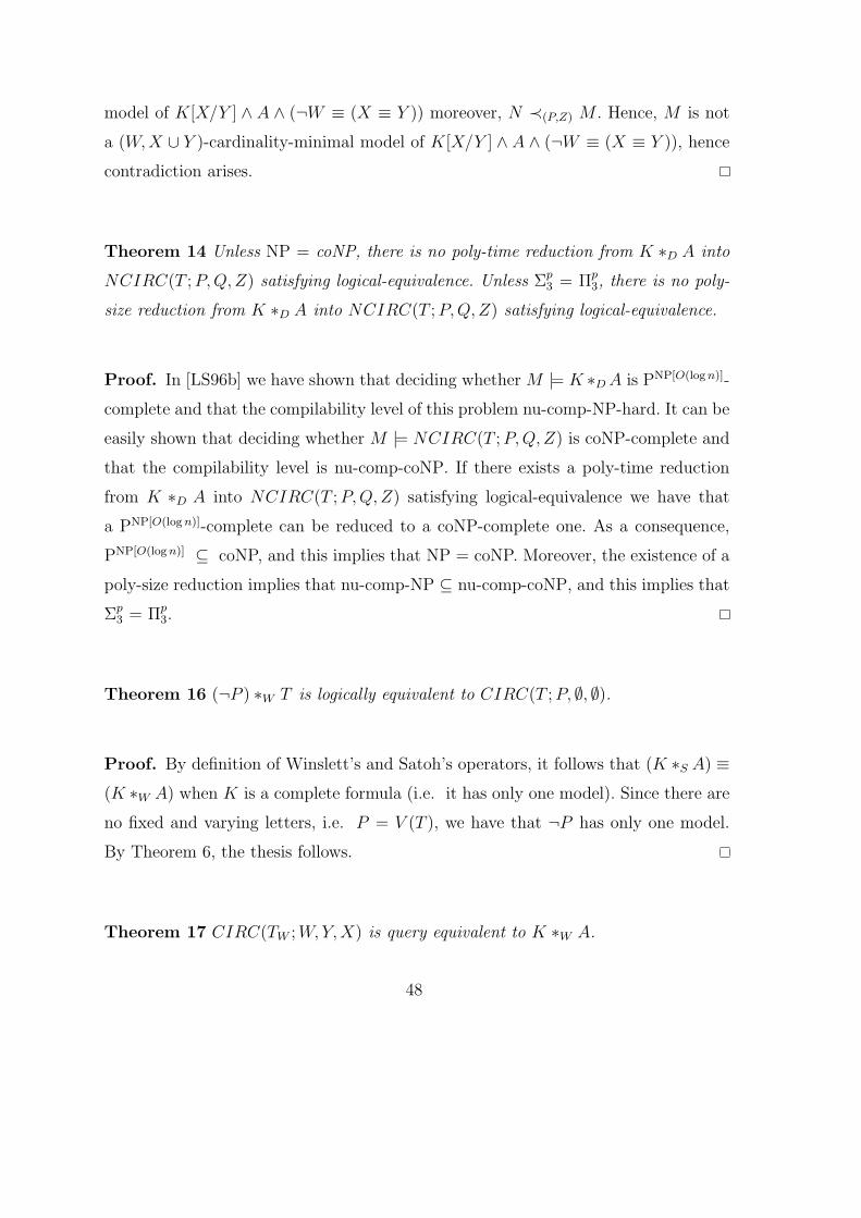
model of K[X/Y ] ∧ A ∧ (¬W ≡ (X ≡ Y )) moreover, N ≺(P,Z) M . Hence, M is not
a (W,X ∪ Y )-cardinality-minimal model of K[X/Y ] ∧ A ∧ (¬W ≡ (X ≡ Y )), hence
contradiction arises.
Theorem 14 Unless NP = coNP, there is no poly-time reduction from K ∗D A into
NCIRC(T ; P, Q, Z) satisfying logical-equivalence. Unless Σp3 = Πp
3, there is no poly-
size reduction from K ∗D A into NCIRC(T ; P,Q, Z) satisfying logical-equivalence.
Proof. In [LS96b] we have shown that deciding whether M |= K ∗D A is PNP[O(log n)]-
complete and that the compilability level of this problem nu-comp-NP-hard. It can be
easily shown that deciding whether M |= NCIRC(T ; P, Q, Z) is coNP-complete and
that the compilability level is nu-comp-coNP. If there exists a poly-time reduction
from K ∗D A into NCIRC(T ; P,Q, Z) satisfying logical-equivalence we have that
a PNP[O(log n)]-complete can be reduced to a coNP-complete one. As a consequence,
PNP[O(log n)] ⊆ coNP, and this implies that NP = coNP. Moreover, the existence of a
poly-size reduction implies that nu-comp-NP ⊆ nu-comp-coNP, and this implies that
Σp3 = Πp
3.
Theorem 16 (¬P ) ∗W T is logically equivalent to CIRC(T ; P, ∅, ∅).
Proof. By definition of Winslett’s and Satoh’s operators, it follows that (K ∗S A) ≡(K ∗W A) when K is a complete formula (i.e. it has only one model). Since there are
no fixed and varying letters, i.e. P = V (T ), we have that ¬P has only one model.
By Theorem 6, the thesis follows.
Theorem 17 CIRC(TW ; W,Y,X) is query equivalent to K ∗W A.
48
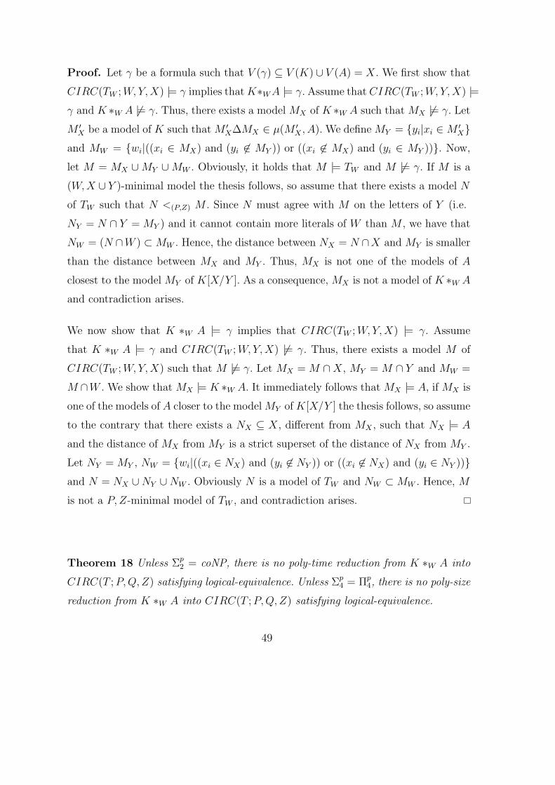
Proof. Let γ be a formula such that V (γ) ⊆ V (K) ∪ V (A) = X. We first show that
CIRC(TW ; W,Y,X) |= γ implies that K∗W A |= γ. Assume that CIRC(TW ; W,Y,X) |=γ and K ∗W A 6|= γ. Thus, there exists a model MX of K ∗W A such that MX 6|= γ. Let
M ′X be a model of K such that M ′
X∆MX ∈ µ(M ′X , A). We define MY = {yi|xi ∈ M ′
X}and MW = {wi|((xi ∈ MX) and (yi 6∈ MY )) or ((xi 6∈ MX) and (yi ∈ MY ))}. Now,
let M = MX ∪MY ∪MW . Obviously, it holds that M |= TW and M 6|= γ. If M is a
(W,X ∪ Y )-minimal model the thesis follows, so assume that there exists a model N
of TW such that N <(P,Z) M . Since N must agree with M on the letters of Y (i.e.
NY = N ∩ Y = MY ) and it cannot contain more literals of W than M , we have that
NW = (N ∩W ) ⊂ MW . Hence, the distance between NX = N ∩X and MY is smaller
than the distance between MX and MY . Thus, MX is not one of the models of A
closest to the model MY of K[X/Y ]. As a consequence, MX is not a model of K ∗W A
and contradiction arises.
We now show that K ∗W A |= γ implies that CIRC(TW ; W,Y, X) |= γ. Assume
that K ∗W A |= γ and CIRC(TW ; W,Y, X) 6|= γ. Thus, there exists a model M of
CIRC(TW ; W,Y,X) such that M 6|= γ. Let MX = M ∩X, MY = M ∩ Y and MW =
M ∩W . We show that MX |= K ∗W A. It immediately follows that MX |= A, if MX is
one of the models of A closer to the model MY of K[X/Y ] the thesis follows, so assume
to the contrary that there exists a NX ⊆ X, different from MX , such that NX |= A
and the distance of MX from MY is a strict superset of the distance of NX from MY .
Let NY = MY , NW = {wi|((xi ∈ NX) and (yi 6∈ NY )) or ((xi 6∈ NX) and (yi ∈ NY ))}and N = NX ∪NY ∪NW . Obviously N is a model of TW and NW ⊂ MW . Hence, M
is not a P, Z-minimal model of TW , and contradiction arises.
Theorem 18 Unless Σp2 = coNP, there is no poly-time reduction from K ∗W A into
CIRC(T ; P, Q, Z) satisfying logical-equivalence. Unless Σp4 = Πp
4, there is no poly-size
reduction from K ∗W A into CIRC(T ; P, Q,Z) satisfying logical-equivalence.
49
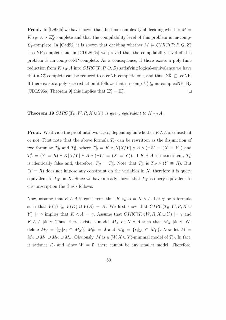
Proof. In [LS96b] we have shown that the time complexity of deciding whether M |=K ∗W A is Σp
2-complete and that the compilability level of this problem is nu-comp-
Σp2-complete. In [Cad92] it is shown that deciding whether M |= CIRC(T ; P,Q, Z)
is coNP-complete and in [CDLS96a] we proved that the compilability level of this
problem is nu-comp-coNP-complete. As a consequence, if there exists a poly-time
reduction from K ∗W A into CIRC(T ; P,Q, Z) satisfying logical-equivalence we have
that a Σp2-complete can be reduced to a coNP-complete one, and thus, Σp
2 ⊆ coNP.
If there exists a poly-size reduction it follows that nu-comp-Σp2 ⊆ nu-comp-coNP. By
[CDLS96a, Theorem 9] this implies that Σp4 = Πp
4.
Theorem 19 CIRC(TB; W,R, X ∪ Y ) is query equivalent to K ∗B A.
Proof. We divide the proof into two cases, depending on whether K∧A is consistent
or not. First note that the above formula TB can be rewritten as the disjunction of
two formulae T 1B and T 2
B, where T 1B = K ∧ K[X/Y ] ∧ A ∧ (¬W ≡ (X ≡ Y )) and
T 2B = (Y ≡ R) ∧ K[X/Y ] ∧ A ∧ (¬W ≡ (X ≡ Y )). If K ∧ A is inconsistent, T 1
B
is identically false and, therefore, TB = T 2B. Note that T 2
B is TW ∧ (Y ≡ R). But
(Y ≡ R) does not impose any constraint on the variables in X, therefore it is query
equivalent to TW on X. Since we have already shown that TW is query equivalent to
circumscription the thesis follows.
Now, assume that K ∧ A is consistent, thus K ∗B A = K ∧ A. Let γ be a formula
such that V (γ) ⊆ V (K) ∪ V (A) = X. We first show that CIRC(TB; W,R, X ∪Y ) |= γ implies that K ∧ A |= γ. Assume that CIRC(TB; W,R,X ∪ Y ) |= γ and
K ∧ A 6|= γ. Thus, there exists a model MX of K ∧ A such that MX 6|= γ. We
define MY = {yi|xi ∈ MX}, MW = ∅ and MR = {ri|yi ∈ MY }. Now let M =
MX ∪MY ∪MW ∪MR. Obviously, M is a (W,X ∪ Y )-minimal model of TB. In fact,
it satisfies TB and, since W = ∅, there cannot be any smaller model. Therefore,
50
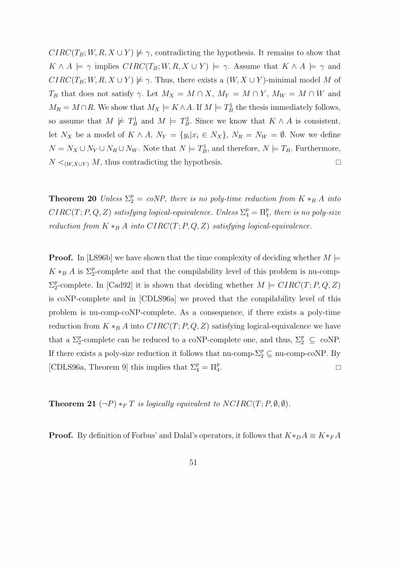
CIRC(TB; W,R, X ∪ Y ) 6|= γ, contradicting the hypothesis. It remains to show that
K ∧ A |= γ implies CIRC(TB; W,R, X ∪ Y ) |= γ. Assume that K ∧ A |= γ and
CIRC(TB; W,R, X ∪ Y ) 6|= γ. Thus, there exists a (W,X ∪ Y )-minimal model M of
TB that does not satisfy γ. Let MX = M ∩ X, MY = M ∩ Y , MW = M ∩ W and
MR = M ∩R. We show that MX |= K∧A. If M |= T 1B the thesis immediately follows,
so assume that M 6|= T 1B and M |= T 2
B. Since we know that K ∧ A is consistent,
let NX be a model of K ∧ A, NY = {yi|xi ∈ NX}, NR = NW = ∅. Now we define
N = NX ∪NY ∪NR ∪NW . Note that N |= T 1B, and therefore, N |= TB. Furthermore,
N <(W,X∪Y ) M , thus contradicting the hypothesis.
Theorem 20 Unless Σp2 = coNP, there is no poly-time reduction from K ∗B A into
CIRC(T ; P, Q, Z) satisfying logical-equivalence. Unless Σp4 = Πp
4, there is no poly-size
reduction from K ∗B A into CIRC(T ; P,Q, Z) satisfying logical-equivalence.
Proof. In [LS96b] we have shown that the time complexity of deciding whether M |=K ∗B A is Σp
2-complete and that the compilability level of this problem is nu-comp-
Σp2-complete. In [Cad92] it is shown that deciding whether M |= CIRC(T ; P,Q, Z)
is coNP-complete and in [CDLS96a] we proved that the compilability level of this
problem is nu-comp-coNP-complete. As a consequence, if there exists a poly-time
reduction from K ∗B A into CIRC(T ; P,Q, Z) satisfying logical-equivalence we have
that a Σp2-complete can be reduced to a coNP-complete one, and thus, Σp
2 ⊆ coNP.
If there exists a poly-size reduction it follows that nu-comp-Σp2 ⊆ nu-comp-coNP. By
[CDLS96a, Theorem 9] this implies that Σp4 = Πp
4.
Theorem 21 (¬P ) ∗F T is logically equivalent to NCIRC(T ; P, ∅, ∅).
Proof. By definition of Forbus’ and Dalal’s operators, it follows that K∗DA ≡ K∗F A
51
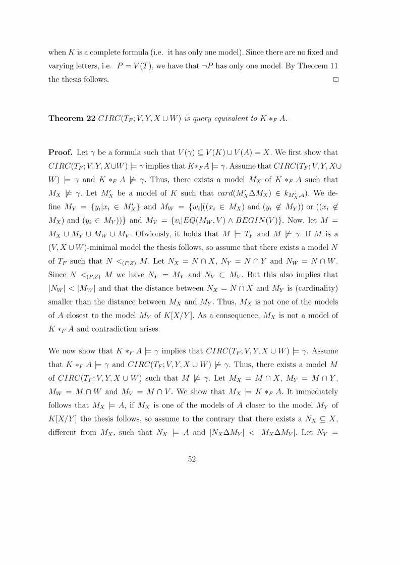
when K is a complete formula (i.e. it has only one model). Since there are no fixed and
varying letters, i.e. P = V (T ), we have that ¬P has only one model. By Theorem 11
the thesis follows.
Theorem 22 CIRC(TF ; V, Y, X ∪W ) is query equivalent to K ∗F A.
Proof. Let γ be a formula such that V (γ) ⊆ V (K) ∪ V (A) = X. We first show that
CIRC(TF ; V, Y, X∪W ) |= γ implies that K∗F A |= γ. Assume that CIRC(TF ; V, Y, X∪W ) |= γ and K ∗F A 6|= γ. Thus, there exists a model MX of K ∗F A such that
MX 6|= γ. Let M ′X be a model of K such that card(M ′
X∆MX) ∈ kM ′X ,A). We de-
fine MY = {yi|xi ∈ M ′X} and MW = {wi|((xi ∈ MX) and (yi 6∈ MY )) or ((xi 6∈
MX) and (yi ∈ MY ))} and MV = {vi|EQ(MW , V ) ∧ BEGIN(V )}. Now, let M =
MX ∪ MY ∪ MW ∪ MV . Obviously, it holds that M |= TF and M 6|= γ. If M is a
(V, X ∪W )-minimal model the thesis follows, so assume that there exists a model N
of TF such that N <(P,Z) M . Let NX = N ∩ X, NY = N ∩ Y and NW = N ∩ W .
Since N <(P,Z) M we have NY = MY and NV ⊂ MV . But this also implies that
|NW | < |MW | and that the distance between NX = N ∩ X and MY is (cardinality)
smaller than the distance between MX and MY . Thus, MX is not one of the models
of A closest to the model MY of K[X/Y ]. As a consequence, MX is not a model of
K ∗F A and contradiction arises.
We now show that K ∗F A |= γ implies that CIRC(TF ; V, Y,X ∪W ) |= γ. Assume
that K ∗F A |= γ and CIRC(TF ; V, Y,X ∪W ) 6|= γ. Thus, there exists a model M
of CIRC(TF ; V, Y, X ∪ W ) such that M 6|= γ. Let MX = M ∩ X, MY = M ∩ Y ,
MW = M ∩ W and MV = M ∩ V . We show that MX |= K ∗F A. It immediately
follows that MX |= A, if MX is one of the models of A closer to the model MY of
K[X/Y ] the thesis follows, so assume to the contrary that there exists a NX ⊆ X,
different from MX , such that NX |= A and |NX∆MY | < |MX∆MY |. Let NY =
52
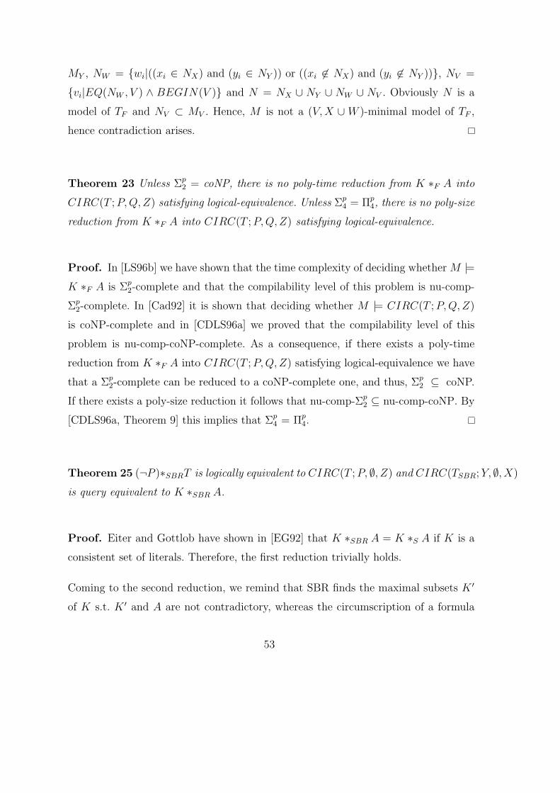
MY , NW = {wi|((xi ∈ NX) and (yi ∈ NY )) or ((xi 6∈ NX) and (yi 6∈ NY ))}, NV =
{vi|EQ(NW , V ) ∧ BEGIN(V )} and N = NX ∪ NY ∪ NW ∪ NV . Obviously N is a
model of TF and NV ⊂ MV . Hence, M is not a (V, X ∪ W )-minimal model of TF ,
hence contradiction arises.
Theorem 23 Unless Σp2 = coNP, there is no poly-time reduction from K ∗F A into
CIRC(T ; P, Q, Z) satisfying logical-equivalence. Unless Σp4 = Πp
4, there is no poly-size
reduction from K ∗F A into CIRC(T ; P, Q,Z) satisfying logical-equivalence.
Proof. In [LS96b] we have shown that the time complexity of deciding whether M |=K ∗F A is Σp
2-complete and that the compilability level of this problem is nu-comp-
Σp2-complete. In [Cad92] it is shown that deciding whether M |= CIRC(T ; P,Q, Z)
is coNP-complete and in [CDLS96a] we proved that the compilability level of this
problem is nu-comp-coNP-complete. As a consequence, if there exists a poly-time
reduction from K ∗F A into CIRC(T ; P,Q, Z) satisfying logical-equivalence we have
that a Σp2-complete can be reduced to a coNP-complete one, and thus, Σp
2 ⊆ coNP.
If there exists a poly-size reduction it follows that nu-comp-Σp2 ⊆ nu-comp-coNP. By
[CDLS96a, Theorem 9] this implies that Σp4 = Πp
4.
Theorem 25 (¬P )∗SBRT is logically equivalent to CIRC(T ; P, ∅, Z) and CIRC(TSBR; Y, ∅, X)
is query equivalent to K ∗SBR A.
Proof. Eiter and Gottlob have shown in [EG92] that K ∗SBR A = K ∗S A if K is a
consistent set of literals. Therefore, the first reduction trivially holds.
Coming to the second reduction, we remind that SBR finds the maximal subsets K ′
of K s.t. K ′ and A are not contradictory, whereas the circumscription of a formula
53
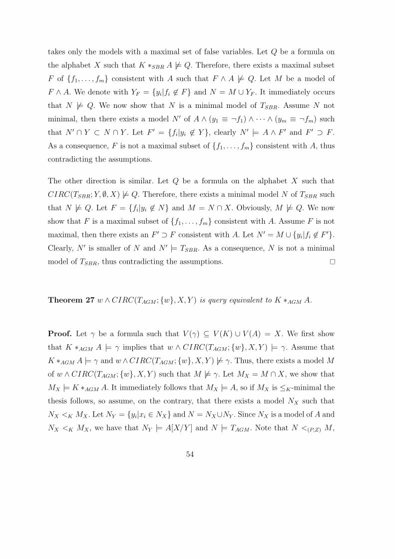
takes only the models with a maximal set of false variables. Let Q be a formula on
the alphabet X such that K ∗SBR A 6|= Q. Therefore, there exists a maximal subset
F of {f1, . . . , fm} consistent with A such that F ∧ A 6|= Q. Let M be a model of
F ∧ A. We denote with YF = {yi|fi 6∈ F} and N = M ∪ YF . It immediately occurs
that N 6|= Q. We now show that N is a minimal model of TSBR. Assume N not
minimal, then there exists a model N ′ of A ∧ (y1 ≡ ¬f1) ∧ · · · ∧ (ym ≡ ¬fm) such
that N ′ ∩ Y ⊂ N ∩ Y . Let F ′ = {fi|yi 6∈ Y }, clearly N ′ |= A ∧ F ′ and F ′ ⊃ F .
As a consequence, F is not a maximal subset of {f1, . . . , fm} consistent with A, thus
contradicting the assumptions.
The other direction is similar. Let Q be a formula on the alphabet X such that
CIRC(TSBR; Y, ∅, X) 6|= Q. Therefore, there exists a minimal model N of TSBR such
that N 6|= Q. Let F = {fi|yi 6∈ N} and M = N ∩ X. Obviously, M 6|= Q. We now
show that F is a maximal subset of {f1, . . . , fm} consistent with A. Assume F is not
maximal, then there exists an F ′ ⊃ F consistent with A. Let N ′ = M ∪ {yi|fi 6∈ F ′}.Clearly, N ′ is smaller of N and N ′ |= TSBR. As a consequence, N is not a minimal
model of TSBR, thus contradicting the assumptions.
Theorem 27 w ∧ CIRC(TAGM ; {w}, X, Y ) is query equivalent to K ∗AGM A.
Proof. Let γ be a formula such that V (γ) ⊆ V (K) ∪ V (A) = X. We first show
that K ∗AGM A |= γ implies that w ∧ CIRC(TAGM ; {w}, X, Y ) |= γ. Assume that
K ∗AGM A |= γ and w∧CIRC(TAGM ; {w}, X, Y ) 6|= γ. Thus, there exists a model M
of w ∧ CIRC(TAGM ; {w}, X, Y ) such that M 6|= γ. Let MX = M ∩X, we show that
MX |= K ∗AGM A. It immediately follows that MX |= A, so if MX is ≤K-minimal the
thesis follows, so assume, on the contrary, that there exists a model NX such that
NX <K MX . Let NY = {yi|xi ∈ NX} and N = NX∪NY . Since NX is a model of A and
NX <K MX , we have that NY |= A[X/Y ] and N |= TAGM . Note that N <(P,Z) M ,
54
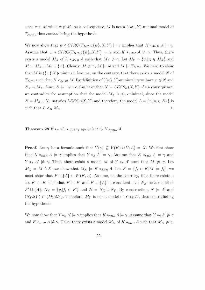
since w ∈ M while w 6∈ M . As a consequence, M is not a ({w}, Y )-minimal model of
TAGM , thus contradicting the hypothesis.
We now show that w ∧ CIRC(TAGM ; {w}, X, Y ) |= γ implies that K ∗AGM A |= γ.
Assume that w ∧ CIRC(TAGM ; {w}, X, Y ) |= γ and K ∗AGM A 6|= γ. Thus, there
exists a model MX of K ∗AGM A such that MX 6|= γ. Let MY = {yi|xi ∈ MX} and
M = MX ∪MY ∪ {w}. Clearly, M 6|= γ, M |= w and M |= TAGM . We need to show
that M is ({w}, Y )-minimal. Assume, on the contrary, that there exists a model N of
TAGM such that N <(P,Z) M . By definition of ({w}, Y )-minimality we have w 6∈ N and
NX = MX . Since N |= ¬w we also have that N |= LESSK(X,Y ). As a consequence,
we contradict the assumption that the model MX is ≤K-minimal, since the model
N = MX ∪NY satisfies LESSK(X, Y ) and therefore, the model L = {xi|yi ∈ NY } is
such that L <K MX .
Theorem 28 Y ∗S A′ is query equivalent to K ∗SBR A.
Proof. Let γ be a formula such that V (γ) ⊆ V (K) ∪ V (A) = X. We first show
that K ∗SBR A |= γ implies that Y ∗S A′ |= γ. Assume that K ∗SBR A |= γ and
Y ∗S A′ 6|= γ. Thus, there exists a model M of Y ∗S A′ such that M 6|= γ. Let
MX = M ∩ X, we show that MX |= K ∗SBR A. Let F = {fi ∈ K|M |= fi}, we
must show that F ∪ {A} ∈ W (K,A). Assume, on the contrary, that there exists a
set F ′ ⊂ K such that F ⊂ F ′ and F ′ ∪ {A} is consistent. Let NX be a model of
F ′ ∪ {A}, NY = {yi|fi ∈ F ′} and N = NX ∪ NY . By construction, N |= A′ and
(NY ∆Y ) ⊂ (MY ∆Y ). Therefore, MY is not a model of Y ∗S A′, thus contradicting
the hypothesis.
We now show that Y ∗S A′ |= γ implies that K ∗SBR A |= γ. Assume that Y ∗S A′ 6|= γ
and K ∗SBR A 6|= γ. Thus, there exists a model MX of K ∗SBR A such that MX 6|= γ.
55
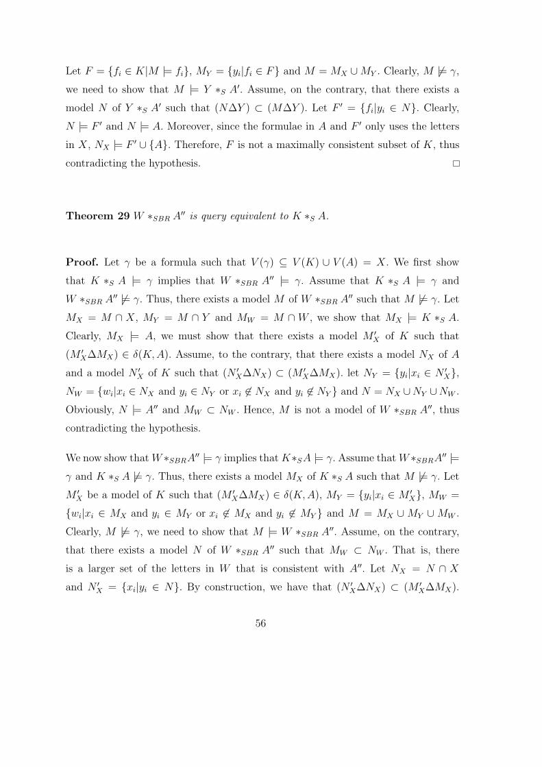
Let F = {fi ∈ K|M |= fi}, MY = {yi|fi ∈ F} and M = MX ∪MY . Clearly, M 6|= γ,
we need to show that M |= Y ∗S A′. Assume, on the contrary, that there exists a
model N of Y ∗S A′ such that (N∆Y ) ⊂ (M∆Y ). Let F ′ = {fi|yi ∈ N}. Clearly,
N |= F ′ and N |= A. Moreover, since the formulae in A and F ′ only uses the letters
in X, NX |= F ′ ∪ {A}. Therefore, F is not a maximally consistent subset of K, thus
contradicting the hypothesis.
Theorem 29 W ∗SBR A′′ is query equivalent to K ∗S A.
Proof. Let γ be a formula such that V (γ) ⊆ V (K) ∪ V (A) = X. We first show
that K ∗S A |= γ implies that W ∗SBR A′′ |= γ. Assume that K ∗S A |= γ and
W ∗SBR A′′ 6|= γ. Thus, there exists a model M of W ∗SBR A′′ such that M 6|= γ. Let
MX = M ∩ X, MY = M ∩ Y and MW = M ∩ W , we show that MX |= K ∗S A.
Clearly, MX |= A, we must show that there exists a model M ′X of K such that
(M ′X∆MX) ∈ δ(K, A). Assume, to the contrary, that there exists a model NX of A
and a model N ′X of K such that (N ′
X∆NX) ⊂ (M ′X∆MX). let NY = {yi|xi ∈ N ′
X},NW = {wi|xi ∈ NX and yi ∈ NY or xi 6∈ NX and yi 6∈ NY } and N = NX ∪NY ∪NW .
Obviously, N |= A′′ and MW ⊂ NW . Hence, M is not a model of W ∗SBR A′′, thus
contradicting the hypothesis.
We now show that W ∗SBRA′′ |= γ implies that K∗SA |= γ. Assume that W ∗SBRA′′ |=γ and K ∗S A 6|= γ. Thus, there exists a model MX of K ∗S A such that M 6|= γ. Let
M ′X be a model of K such that (M ′
X∆MX) ∈ δ(K, A), MY = {yi|xi ∈ M ′X}, MW =
{wi|xi ∈ MX and yi ∈ MY or xi 6∈ MX and yi 6∈ MY } and M = MX ∪ MY ∪ MW .
Clearly, M 6|= γ, we need to show that M |= W ∗SBR A′′. Assume, on the contrary,
that there exists a model N of W ∗SBR A′′ such that MW ⊂ NW . That is, there
is a larger set of the letters in W that is consistent with A′′. Let NX = N ∩ X
and N ′X = {xi|yi ∈ N}. By construction, we have that (N ′
X∆NX) ⊂ (M ′X∆MX).
56
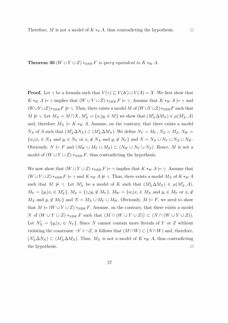
Therefore, M is not a model of K ∗S A, thus contradicting the hypothesis.
Theorem 30 (W ∪ Y ∪ Z) ∗SBR F is query equivalent to K ∗W A.
Proof. Let γ be a formula such that V (γ) ⊆ V (K) ∪ V (A) = X. We first show that
K ∗W A |= γ implies that (W ∪ Y ∪ Z) ∗SBR F |= γ. Assume that K ∗W A |= γ and
(W∪Y ∪Z)∗SBRF 6|= γ. Thus, there exists a model M of (W∪Y ∪Z)∗SBRF such that
M 6|= γ. Let MX = M ∩X, M ′X = {xi|yi ∈ M} we show that (M ′
X∆MX) ∈ µ(M ′X , A)
and, therefore MX |= K ∗W A. Assume, on the contrary, that there exists a model
NX of A such that (M ′X∆NX) ⊂ (M ′
X∆MX). We define NY = MY , NZ = MZ , NW =
{wi|xi ∈ NX and yi ∈ NY or xi 6∈ NX and yi 6∈ NY } and N = NX ∪NY ∪NZ ∪NW .
Obviously, N |= F and (MW ∪ MY ∪ MZ) ⊂ (NW ∪ NY ∪ NZ). Hence, M is not a
model of (W ∪ Y ∪ Z) ∗SBR F , thus contradicting the hypothesis.
We now show that (W ∪ Y ∪ Z) ∗SBR F |= γ implies that K ∗W A |= γ. Assume that
(W ∪Y ∪Z)∗SBR F |= γ and K ∗W A 6|= γ. Thus, there exists a model MX of K ∗W A
such that M 6|= γ. Let M ′X be a model of K such that (M ′
X∆MX) ∈ µ(M ′X , A),
MY = {yi|xi ∈ M ′X}, MZ = {zi|yi 6∈ MY }, MW = {wi|xi ∈ MX and yi ∈ MY or xi 6∈
MX and yi 6∈ MY } and N = MX ∪MY ∪MW . Obviously, M |= F , we need to show
that M |= (W ∪ Y ∪ Z) ∗SBR F . Assume, on the contrary, that there exists a model
N of (W ∪ Y ∪ Z) ∗SBR F such that (M ∩ (W ∪ Y ∪ Z)) ⊂ (N ∩ (W ∪ Y ∪ Z)).
Let N ′X = {yi|xi ∈ NY }. Since N cannot contain more literals of Y or Z without
violating the constraint ¬Y ∨¬Z, it follows that (M ∩W ) ⊂ (N ∩W ) and, therefore,
(N ′X∆NX) ⊂ (M ′
X∆MX). Thus, MX is not a model of K ∗W A, thus contradicting
the hypothesis.
57
Theorem 31 Unless Σp2 = coNP, there is no poly-time reduction from K∗SA (K∗W A)
into K ′ ∗SBR A′ satisfying logical-equivalence. Unless Σp4 = Πp
4, there is no poly-size
reduction from K ∗S A (K ∗W A) into K ′ ∗SBR A′ satisfying logical-equivalence.
Proof. In [LS96b] we have shown that the time complexity of deciding whether
M |= K ∗S A and M |= K ∗W A is Σp2-complete and that the compilability level of
this problem is nu-comp-Σp2-complete, while the time complexity of deciding whether
M |= K ∗SBR A is coNP-complete and that the compilability level of this problem
is nu-comp-coNP-complete. As a consequence, if there exists a poly-time reduction
from K ∗S A (K ∗W A) into K ′ ∗SBR A′ satisfying logical-equivalence we have that
a Σp2-complete can be reduced to a coNP-complete one, and thus, Σp
2 ⊆ coNP. If
there exists a poly-size reduction it follows that nu-comp-Σp2 ⊆ nu-comp-coNP. By
[CDLS96a, Theorem 9] this implies that Σp4 = Πp
4.
58


![Authorship Attribution through Character Substrings (and vice versa) [in French]](https://img.pdfslide.net/doc/110x75/6348f0a3031992cdcf024bae/authorship-attribution-through-character-substrings-and-vice-versa-in-french.jpg)


