Embed Size (px)
Citation preview
UNIVERSITY OF GREENWICH
Reducing Deadline Miss Rate for GridWorkloads running in Virtual Machines: a
deadline-aware and adaptive approach
by
Omer Khalid
A thesis submitted in fulfillment for thedegree of Doctor of Philosophy
in the
School of Computing and Mathematical Sciences
August 2011

All of our individual efforts forms the collective basis of human
progress and development.
I wouldn’t have become what I am now without the sparkling
love of my grandmother Janat Bibi, early educational training
given to me by my uncle Shamim Ahmed and unwavering trust
of my father Bashir Ahmed Khalid in me over the course of my
life.
This work is dedicated to all three of them!
i

Abstract
This thesis explores three major areas of research; integration of virutalization into sci-
entific grid infrastructures, evaluation of the virtualization overhead on HPC grid job’s
performance, and optimization of job execution times to increase their throughput by
reducing job deadline miss rate.
Integration of the virtualization into the grid to deploy on-demand virtual machines
for jobs in a way that is transparent to the end users and have minimum impact on
the existing system poses a significant challenge. This involves the creation of virtual
machines, decompression of the operating system image, adapting the virtual environ-
ment to satisfy software requirements of the job, constant update of the job state once
it’s running with out modifying batch system or existing grid middleware, and finally
bringing the host machine back to a consistent state.
To facilitate this research, an existing and in production pilot job framework has been
modified to deploy virtual machines on demand on the grid using virtualization ad-
ministrative domain to handle all I/O to increase network throughput. This approach
limits the change impact on the existing grid infrastructure while leveraging the exe-
cution and performance isolation capabilities of virtualization for job execution. This
work led to evaluation of various scheduling strategies used by the Xen hypervisor to
measure the sensitivity of job performance to the amount of CPU and memory allo-
cated under various configurations.
However, virtualization overhead is also a critical factor in determining job execution
times. Grid jobs have a diverse set of requirements for machine resources such as CPU,
Memory, Network and have inter-dependencies on other jobs in meeting their dead-
lines since the input of one job can be the output from the previous job. A novel re-
source provisioning model was devised to decrease the impact of virtualization over-
head on job execution.
Finally, dynamic deadline-aware optimization algorithms were introduced using ex-
ponential smoothing and rate limiting to predict job failure rates based on static and
dynamic virtualization overhead. Statistical techniques were also integrated into the
optimization algorithm to flag jobs that are at risk to miss their deadlines, and taking
preventive action to increase overall job throughput.

Acknowledgements
I would like to first of all thank you my Phd supervisors; Dr. Miltos Petridis and Dr.
Richard Anthony for their excellent supervision during the course of this thesis re-
search.
I would like to especially thank Dr. Richard Anthony for his rigorous feedback during
the write-up and final phase of my thesis preparations.
I would like to thank CERN, and my CERN supervisor Dr. Markus Schulz for provid-
ing me with an excellent research environment and the resources I needed for continu-
ing my work.
During the course of this research, brainstorming with more experienced researchers
was also very important for me to fully understand the complexity of CERN’s com-
puting Grid and ATLAS experiment’s job execution frameworks. I would like to thank
developers from ATLAS collaboration for providing me with the needed documenta-
tion and answering my questions. There were many people involved in this process
but particularly I would like to thank Paul Nilsson.
I would also like to thank Dr. Kate Keahey from Argonne National Laboratory, USA,
for her valuable input and critical questioning on my initial ideas related to ATLAS
workload optimizations which enabled me to dig deeper, and learn various aspect of
the research process about defining the problem statement.
I would like to thank Dr. Ivo Majelovic for pointing me to various smoothing and rate
limiting algorithms that led me to learn about them, and eventually applying them to
the research work presented in this thesis.
I would like to thank my two good friends from CERN; Angelos Molfetas and Ozgur
Cobanoglu - for brainstorming with me on many occasions during the last two years,
and challenging my ideas/assumptions through discussions. I learnt great deal from
their insights from the approaches they developed in their research domains of genetic
algorithms and electronic design respectively.
I would like to especially thank again Angelos Melfetas for proof reading my thesis
and providing me with valuable feedback to improve certain structural aspects of this
thesis.
Finally I would like to thank my family and relatives for supporting me and providing
me with the moral encouragement, and also tolerating my long absences while I was
busy with the write-up of this thesis.
iii

Publications
The research work presented in this thesis has been accepted in numerous peer re-
viewed conferences.
1. vGrid: Virtual Machine Life Cycle Management [1]: This publication explores the in-
tegration of virtualization deployment tools in the grid infrastructure and presents
the architecture of one such implementation namely vGrid tool. It’s contents are
included in chapter 3 and 5.
2. Enabling Virtual PanDA pilot for ATLAS [2]: This publication extended the work
done in the previous document, and worked towards integrating vGrid virtual
machine deployment engine into an existing ATLAS framework called PanDA
pilot job framework to automate the virtual machine creation process on worker
nodes. This covers the contents in chapter 5.
3. Executing ATLAS jobs in Virtual Machine [3]: This publication presented an im-
plementation study of running ATLAS jobs in virtual machines. This covers the
contents in chapter 5.
4. Enabling and Optimizing Pilot Jobs using Xen Virtual Machines for HPC Grid Applica-
tions [4]: This publication highlighted the research done in the previous work. A
preliminary study of evaluation of ATLAS workloads by executing them in vir-
tual machines was conduced and it presented optimization techniques for Xen
hypervisor to increase virtual machine performance. It highlighted the impact of
CPU and memory misallocation on job execution times. This covers the content
in chapter 2, 3 and 5.
5. Dynamic Scheduling of Virtual Machines running HPC workloads in Scientific Grids
[5]: This publication covers the preliminary research conducted into optimization
of deadline miss rate of ATLAS jobs in virtual machines using various scheduling
techniques. This covers the contents in chapter 2 and 6.
6. Deadline Aware Virtual Machine Scheduler for Scientific Grids and Cloud Computing
[6]: This publication develops on the previous work, and extended the research
done into adaptive algorithm based on rate limiting and statistical techniques for
reducing job deadline miss rate and increasing job throughput rate. This covers
the contents in 3, 6 and 8.
iv

Contents
Abstract ii
Acknowledgements iii
Publications iv
List of Figures ix
List of Tables xi
Abbreviations xii
1 Introduction 11.1 Research Questions . . . . . . . . . . . . . . . . . . . . . . . . . . . . . . . 31.2 Research Objectives . . . . . . . . . . . . . . . . . . . . . . . . . . . . . . . 41.3 Research Method . . . . . . . . . . . . . . . . . . . . . . . . . . . . . . . . 51.4 Thesis Structure . . . . . . . . . . . . . . . . . . . . . . . . . . . . . . . . . 71.5 Contribution . . . . . . . . . . . . . . . . . . . . . . . . . . . . . . . . . . . 9
2 Fundamental Concepts 102.1 Virtualization Technology . . . . . . . . . . . . . . . . . . . . . . . . . . . 11
2.1.1 Advantages of Virtualization . . . . . . . . . . . . . . . . . . . . . 122.1.2 Under the hood . . . . . . . . . . . . . . . . . . . . . . . . . . . . . 132.1.3 Software Virtualization . . . . . . . . . . . . . . . . . . . . . . . . 162.1.4 Hardware Virtualization . . . . . . . . . . . . . . . . . . . . . . . . 17
2.2 Large Scale Distributed Computing . . . . . . . . . . . . . . . . . . . . . . 182.2.1 Grid and it’s Architecture . . . . . . . . . . . . . . . . . . . . . . . 192.2.2 Grid Middleware . . . . . . . . . . . . . . . . . . . . . . . . . . . . 21
2.2.2.1 gLite Architecture . . . . . . . . . . . . . . . . . . . . . . 212.2.3 ATLAS Computing . . . . . . . . . . . . . . . . . . . . . . . . . . . 24
2.2.3.1 Job Submission Mechanisms . . . . . . . . . . . . . . . . 242.2.4 Job Scheduling . . . . . . . . . . . . . . . . . . . . . . . . . . . . . 252.2.5 Grid Sites Constraints . . . . . . . . . . . . . . . . . . . . . . . . . 26
2.3 Summary . . . . . . . . . . . . . . . . . . . . . . . . . . . . . . . . . . . . . 28
v

Contents
3 Literature Review 293.1 Virtualization in the Infrastructure . . . . . . . . . . . . . . . . . . . . . . 31
3.1.1 Virtualized Grid Computing . . . . . . . . . . . . . . . . . . . . . 313.1.1.1 Resource Management . . . . . . . . . . . . . . . . . . . 313.1.1.2 Deployment Techniques . . . . . . . . . . . . . . . . . . 35
3.1.2 Rising ”Clouds” . . . . . . . . . . . . . . . . . . . . . . . . . . . . . 413.2 Virtualization and Performance Challenges . . . . . . . . . . . . . . . . . 46
3.2.1 Overhead Diagnosis and Optimization . . . . . . . . . . . . . . . 463.2.1.1 Diagnostic and Monitoring . . . . . . . . . . . . . . . . . 473.2.1.2 Approaches . . . . . . . . . . . . . . . . . . . . . . . . . . 49
3.3 Infrastructure Management through Virtualization . . . . . . . . . . . . . 513.3.1 Live Migration of Virtual Machines . . . . . . . . . . . . . . . . . 513.3.2 Green Computing . . . . . . . . . . . . . . . . . . . . . . . . . . . 543.3.3 Security implications of Virtualization . . . . . . . . . . . . . . . . 55
3.4 Scheduling and Virtualization . . . . . . . . . . . . . . . . . . . . . . . . . 583.5 Summary . . . . . . . . . . . . . . . . . . . . . . . . . . . . . . . . . . . . . 61
4 Theoretical Concepts of Optimization Algorithms 644.1 Theory and Simulation Design . . . . . . . . . . . . . . . . . . . . . . . . 65
4.1.1 Assumptions and Hypothesis . . . . . . . . . . . . . . . . . . . . . 654.1.1.1 Assumptions . . . . . . . . . . . . . . . . . . . . . . . . . 664.1.1.2 Hypothesis . . . . . . . . . . . . . . . . . . . . . . . . . . 67
4.1.2 Software Simulator Architecture . . . . . . . . . . . . . . . . . . . 674.2 Algorithms Design and Architecture . . . . . . . . . . . . . . . . . . . . . 68
4.2.1 Virtual Execution Time . . . . . . . . . . . . . . . . . . . . . . . . . 694.2.2 Deadline Constraints . . . . . . . . . . . . . . . . . . . . . . . . . . 704.2.3 Performance Metrics . . . . . . . . . . . . . . . . . . . . . . . . . . 714.2.4 Execution Flow of Algorithms . . . . . . . . . . . . . . . . . . . . 724.2.5 Real-Time Failure Rate . . . . . . . . . . . . . . . . . . . . . . . . . 764.2.6 Scheduling Strategies . . . . . . . . . . . . . . . . . . . . . . . . . 79
4.3 Summary . . . . . . . . . . . . . . . . . . . . . . . . . . . . . . . . . . . . . 80
5 ATLAS Job Performance Experiments 815.1 Existing ATLAS System . . . . . . . . . . . . . . . . . . . . . . . . . . . . 82
5.1.1 PanDA Architecture . . . . . . . . . . . . . . . . . . . . . . . . . . 825.1.2 Virtualization in PanDA Pilot . . . . . . . . . . . . . . . . . . . . . 83
5.1.2.1 vGrid Deployment Engine . . . . . . . . . . . . . . . . . 835.1.2.2 Virtualization Interfaces . . . . . . . . . . . . . . . . . . 855.1.2.3 Modification to PanDA Pilot . . . . . . . . . . . . . . . . 86
5.2 Preliminary Evaluation Studies . . . . . . . . . . . . . . . . . . . . . . . . 875.2.1 Evaluation Metric . . . . . . . . . . . . . . . . . . . . . . . . . . . . 885.2.2 Approach and Method . . . . . . . . . . . . . . . . . . . . . . . . . 895.2.3 Experiment Design . . . . . . . . . . . . . . . . . . . . . . . . . . . 90
5.2.3.1 Setup . . . . . . . . . . . . . . . . . . . . . . . . . . . . . 905.2.3.2 Xen Parameters . . . . . . . . . . . . . . . . . . . . . . . 90
5.3 Results . . . . . . . . . . . . . . . . . . . . . . . . . . . . . . . . . . . . . . 915.3.1 Network I/O Performance . . . . . . . . . . . . . . . . . . . . . . 92
vi

Contents
5.3.2 Impact of CPU Parameters . . . . . . . . . . . . . . . . . . . . . . 945.3.3 Impact of Memory . . . . . . . . . . . . . . . . . . . . . . . . . . . 97
5.4 Summary . . . . . . . . . . . . . . . . . . . . . . . . . . . . . . . . . . . . . 100
6 Optimization Experiments for Deadline Miss Rate 1026.1 Experimental Design and Rational . . . . . . . . . . . . . . . . . . . . . . 103
6.1.1 Understanding the Results . . . . . . . . . . . . . . . . . . . . . . 1036.1.2 Experimental Design . . . . . . . . . . . . . . . . . . . . . . . . . . 106
6.2 Results . . . . . . . . . . . . . . . . . . . . . . . . . . . . . . . . . . . . . . 1076.2.1 Training Phase . . . . . . . . . . . . . . . . . . . . . . . . . . . . . 107
6.2.1.1 Resource Optimization . . . . . . . . . . . . . . . . . . . 1076.2.1.2 Alpha and Delta x Optimization . . . . . . . . . . . . . . 109
6.2.2 Threshold Determination . . . . . . . . . . . . . . . . . . . . . . . 1126.2.2.1 Delta Adaptation Algorithm . . . . . . . . . . . . . . . . 1126.2.2.2 Probabilistic Adaption Algorithm . . . . . . . . . . . . . 115
6.2.3 Steady Phase . . . . . . . . . . . . . . . . . . . . . . . . . . . . . . 1176.2.3.1 System Performance . . . . . . . . . . . . . . . . . . . . . 1176.2.3.2 Algorithmic Execution Performance . . . . . . . . . . . 122
6.3 Summary . . . . . . . . . . . . . . . . . . . . . . . . . . . . . . . . . . . . . 124
7 Conclusion 126
8 Future Work 130
A CERN and LHC Machine 132A.1 CERN . . . . . . . . . . . . . . . . . . . . . . . . . . . . . . . . . . . . . . . 132A.2 Large Hadron Collider . . . . . . . . . . . . . . . . . . . . . . . . . . . . . 133
B ATLAS Experiment 135B.1 Background . . . . . . . . . . . . . . . . . . . . . . . . . . . . . . . . . . . 135B.2 Job Types . . . . . . . . . . . . . . . . . . . . . . . . . . . . . . . . . . . . . 136
C ATLAS Feasibility Results 138C.1 Experimental Setup . . . . . . . . . . . . . . . . . . . . . . . . . . . . . . . 138
C.1.1 Specification . . . . . . . . . . . . . . . . . . . . . . . . . . . . . . . 138C.1.2 Test Definition . . . . . . . . . . . . . . . . . . . . . . . . . . . . . . 138
C.1.2.1 Physical Baseline . . . . . . . . . . . . . . . . . . . . . . . 139C.1.2.2 Virtual Baseline . . . . . . . . . . . . . . . . . . . . . . . 139C.1.2.3 Memory Optimization . . . . . . . . . . . . . . . . . . . 139C.1.2.4 CPU Core Optimization . . . . . . . . . . . . . . . . . . . 139C.1.2.5 CPU Scheduling Optimization . . . . . . . . . . . . . . . 140C.1.2.6 Network Optimization . . . . . . . . . . . . . . . . . . . 140
C.2 Summarized Data . . . . . . . . . . . . . . . . . . . . . . . . . . . . . . . . 142C.3 Raw Data . . . . . . . . . . . . . . . . . . . . . . . . . . . . . . . . . . . . . 143C.4 Network Throughput Data . . . . . . . . . . . . . . . . . . . . . . . . . . 146
vii

Contents
D PanDA Pilot Code 147D.1 Core Pilot Application . . . . . . . . . . . . . . . . . . . . . . . . . . . . . 147
D.1.1 Status Parameters . . . . . . . . . . . . . . . . . . . . . . . . . . . . 147D.1.2 Input Parameters . . . . . . . . . . . . . . . . . . . . . . . . . . . . 148D.1.3 Staging-In . . . . . . . . . . . . . . . . . . . . . . . . . . . . . . . . 149D.1.4 Clean-up Phase . . . . . . . . . . . . . . . . . . . . . . . . . . . . . 149
D.2 RunJob Pilot Application . . . . . . . . . . . . . . . . . . . . . . . . . . . . 150D.2.1 Job Execution Phase . . . . . . . . . . . . . . . . . . . . . . . . . . 150D.2.2 Status Update . . . . . . . . . . . . . . . . . . . . . . . . . . . . . . 151
E Scheduling Algorithms Code 152E.1 Dynamic Virtualization . . . . . . . . . . . . . . . . . . . . . . . . . . . . . 152
E.1.1 Overhead Prediction . . . . . . . . . . . . . . . . . . . . . . . . . . 152E.1.2 Real Job Progress . . . . . . . . . . . . . . . . . . . . . . . . . . . . 154E.1.3 Job Deadline Validation . . . . . . . . . . . . . . . . . . . . . . . . 154
E.2 Adaptive Algorithms . . . . . . . . . . . . . . . . . . . . . . . . . . . . . . 155E.2.1 Failure Rate Calculation . . . . . . . . . . . . . . . . . . . . . . . . 155E.2.2 x Threshold Adaptation . . . . . . . . . . . . . . . . . . . . . . . . 156E.2.3 Statistical Determination . . . . . . . . . . . . . . . . . . . . . . . . 158E.2.4 Probabilistic x Adaptation . . . . . . . . . . . . . . . . . . . . . . . 159
F Resource Utilization 160F.1 Results . . . . . . . . . . . . . . . . . . . . . . . . . . . . . . . . . . . . . . 160
F.1.1 CPU to Memory ratio: 1 to 1 . . . . . . . . . . . . . . . . . . . . . 160F.1.2 CPU to Memory ratio: 1 to 1.5 . . . . . . . . . . . . . . . . . . . . 163F.1.3 CPU to Memory ratio: 1 to 2 . . . . . . . . . . . . . . . . . . . . . 165F.1.4 CPU to Memory ratio: 1 to 3 . . . . . . . . . . . . . . . . . . . . . 167
G Alpha and Delta x Training 169G.1 Training Results . . . . . . . . . . . . . . . . . . . . . . . . . . . . . . . . . 169
G.1.1 α1=0.01 . . . . . . . . . . . . . . . . . . . . . . . . . . . . . . . . . . 169G.1.2 α2=0.05 . . . . . . . . . . . . . . . . . . . . . . . . . . . . . . . . . . 169G.1.3 α3=0.1 . . . . . . . . . . . . . . . . . . . . . . . . . . . . . . . . . . 169G.1.4 ∆x1=0.05 . . . . . . . . . . . . . . . . . . . . . . . . . . . . . . . . . 173G.1.5 ∆x2=0.1 . . . . . . . . . . . . . . . . . . . . . . . . . . . . . . . . . 174G.1.6 ∆x3=0.2 . . . . . . . . . . . . . . . . . . . . . . . . . . . . . . . . . 175
Bibliography 176
Glossary 192
Index 197
viii

List of Figures
2.1 IA32 Privilege . . . . . . . . . . . . . . . . . . . . . . . . . . . . . . . . . . 132.2 Virtualized Guest OS Privilege Model . . . . . . . . . . . . . . . . . . . . 142.3 ENIAC Computer . . . . . . . . . . . . . . . . . . . . . . . . . . . . . . . . 182.4 Tianhe-1A Supercomputer . . . . . . . . . . . . . . . . . . . . . . . . . . . 192.5 gLite Middleware Architecture . . . . . . . . . . . . . . . . . . . . . . . . 23
4.1 VM Simulator Architecture . . . . . . . . . . . . . . . . . . . . . . . . . . 684.2 Adaptive XThresh algorithm . . . . . . . . . . . . . . . . . . . . . . . . . . 744.3 Adaptive XThresh algorithm . . . . . . . . . . . . . . . . . . . . . . . . . . 76
5.1 Pilot Jobs Overview . . . . . . . . . . . . . . . . . . . . . . . . . . . . . . . 825.2 PanDA Pilot Physical Architecture . . . . . . . . . . . . . . . . . . . . . . 845.3 vGrid Deployment Agent . . . . . . . . . . . . . . . . . . . . . . . . . . . 855.4 VIRM Interfaces . . . . . . . . . . . . . . . . . . . . . . . . . . . . . . . . . 875.5 Virtual PanDA Pilot Execution . . . . . . . . . . . . . . . . . . . . . . . . 885.6 Memory Impact on Dom0 Network Throughput . . . . . . . . . . . . . . 935.7 Xen Scheduling Strategies . . . . . . . . . . . . . . . . . . . . . . . . . . . 965.8 Optimization of Xen Scheduling Parameters . . . . . . . . . . . . . . . . 975.9 VM Physical Memory Performance . . . . . . . . . . . . . . . . . . . . . . 995.10 VM Virtual Memory Performance . . . . . . . . . . . . . . . . . . . . . . . 100
6.1 Overview of Algorithmic Performance and Failure Rate Evolution . . . 1056.2 System Performance for Resource Training . . . . . . . . . . . . . . . . . 1096.3 Global Alpha and Delta x Training Results . . . . . . . . . . . . . . . . . 1116.4 Job success rate and termination rate for XThresh . . . . . . . . . . . . . . 1146.5 XThresh and failure rate evolution for PA algorithm . . . . . . . . . . . . 1166.6 System Performance for NO, SO and DO algorithms . . . . . . . . . . . 1186.7 System Performance for DA and PA algorithms . . . . . . . . . . . . . . 1206.8 DA and PA x Threshold and Failure rate evolution . . . . . . . . . . . . . 1216.9 Algorithm time performance comparison . . . . . . . . . . . . . . . . . . 123
A.1 LHC Experiment . . . . . . . . . . . . . . . . . . . . . . . . . . . . . . . . 133
B.1 ATLAS Experiment . . . . . . . . . . . . . . . . . . . . . . . . . . . . . . . 136
F.1 System Performance: Resource Ratio 1 . . . . . . . . . . . . . . . . . . . . 161F.2 Resource Utilization for Ratio 1:1 . . . . . . . . . . . . . . . . . . . . . . . 162F.3 System Performance: Resource Ratio 2 . . . . . . . . . . . . . . . . . . . 163F.4 Resource Utilization for Ratio 1:1.5 . . . . . . . . . . . . . . . . . . . . . . 164
ix

List of Figures
F.5 System Performance: Resource Ratio 3 . . . . . . . . . . . . . . . . . . . . 165F.6 Resource Utilization for Ratio 1:2 . . . . . . . . . . . . . . . . . . . . . . . 166F.7 System Performance: Resource Ratio 4 . . . . . . . . . . . . . . . . . . . . 167F.8 Resource Utilization for Ratio 1:3 . . . . . . . . . . . . . . . . . . . . . . . 168
G.1 Training Results for α1=0.01 . . . . . . . . . . . . . . . . . . . . . . . . . . 170G.2 Training Results for α2=0.05 . . . . . . . . . . . . . . . . . . . . . . . . . . 171G.3 Training Results for α3=0.1 . . . . . . . . . . . . . . . . . . . . . . . . . . . 172G.4 Training Results for ∆x=0.1 . . . . . . . . . . . . . . . . . . . . . . . . . . 173G.5 Training Results for ∆x=0.15 . . . . . . . . . . . . . . . . . . . . . . . . . . 174G.6 Training Results for ∆x=0.2 . . . . . . . . . . . . . . . . . . . . . . . . . . 175
x

List of Tables
3.1 Grid vs Cloud Computing . . . . . . . . . . . . . . . . . . . . . . . . . . . 43
5.1 VM Network Throughput . . . . . . . . . . . . . . . . . . . . . . . . . . . 945.2 Impact of Xen CPU capping on Job Performance . . . . . . . . . . . . . . 955.3 Impact of Memory Size on ATLAS Job Performance . . . . . . . . . . . . 98
6.1 Alpha and Delta Training Results . . . . . . . . . . . . . . . . . . . . . . . 1116.2 Probability Threshold Comparison . . . . . . . . . . . . . . . . . . . . . . 1156.3 DA and PA Performance Comparison . . . . . . . . . . . . . . . . . . . . 119
B.1 ATLAS Job Types . . . . . . . . . . . . . . . . . . . . . . . . . . . . . . . . 137
C.1 Test Configurations for ATLAS Job Performance . . . . . . . . . . . . . . 141C.2 Summarized Results for ATLAS Jobs . . . . . . . . . . . . . . . . . . . . . 142C.3 Raw Data for the ATLAS Job Performance . . . . . . . . . . . . . . . . . . 145C.4 Network Throughput for ATLAS Jobs . . . . . . . . . . . . . . . . . . . . 146
xi

Abbreviations
AAA Authorization, Authentication and Accounting System
ALICE A Large Ion Collider Experiment
ATLAS A Toroidal LHC Apparatus
BVT Borrowed Virtual Time
BQP Batch Queue Prediction
CapEx Capital Expenditure
CE Computing Element
CERN European Organization for Nuclear Research
(French: Conseil European pour la Recherche Nuclaire)
CMS Compact Muon Solenoid
CPU Central Processing Unit
DIRAC Distributed Infrastructure with Remote Agent Control
DMS Data Management System
DNS Domain Name Server
ENIAC Electronic Numerical Integrator and Computer
GRAM Grid Resource Allocation and Management
HEP High Energy Physics
HPC High Performance Computing
HVM Hardware based Virtual Machine
IaaS Infrastructure as a Service
IMA Integrity Management Architecture
IBM International Business Machines
IDD Isolated Device Domains
IP Internet Protocol
IS Information System
xii

Abbreviations
JVM Java Virtual Machine
LB Logging and Bookkeeping service
LCG Large Hadron Collider Computer Grid
LHC Large Hadron Collider
LHCb Large Hadron Collider beauty
LVM Logical Volume Manager
LRM Local Resource Manager
NIC Network Interface Card
MON Monitoring Services
PanDA Production And Distributed Analysis system
OS Operating System
PaaS Platform as a Service
QBETS Queue Bounds Estimation from Time Series
RAM Random Access Memory
REST Representational State Transfer
SaaS Software as a Service
SE Storage Element
SEDF Simple Earliest Deadline First
SLC Scientific Linux CERN
TPM Trusted Platform Module
UI User Interface
VC Volunteer Computing
VDT Virtual Data Toolkit
VIRM VIrtualization Resource Management
VM Virtual Machine
VMM Virtual Machine Monitor
VO Virtual Organization
WAN Wide-Area Network
WMS Workload Management System
WM Workload Manager
WN Worker Node
xiii

Chapter 1
Introduction
“Nothing in life is to be feared, it’s only to be understood.”
Marie Curie
Grid computing is an infrastructure where computing resources are highly distributed
geographically spanning over very many data centers, and provides sharing of re-
sources for diverse community of users in decentralised fashion [7]. Grid computing
is an evolutionary upward step from cluster computing, which was very popular in
1990’s, as the main computing platform for scientific applications [8, 9].
In the past few years, under utilization of server resource in data-centers led to the
uptake of virtualization technology to increase their resource utilization which leads
to lower support costs, higher mobility of the applications, higher fault tolerance with
lower Capital Expenditure (CapEx) [10]. ” At a high level, virtualization means turning
physical resources into logical ones. It’s a layer of abstraction. In this sense, it’s something
that the IT industry has been doing for essentially forever. For example, when you write a file to
disk, you’re taking advantage of many software and hardware abstractions such as the operating
system’s file system and logical block addressing in the disk controller. Collectively, each of these
virtualization levels simplify how what’s above interacts with what’s below” [11].
Deployment of operating system virtualization on the Grid has also been an active
arena of research since the virtualization technology became an established desktop
1

Chapter 1 Introduction
tool [12]. This is particularly challenging for large research organizations like Euro-
pean Organization for Nuclear Research (CERN) where thousands of servers or worker
nodes have to be constantly configured for large set of software environments: if a plat-
form can be configured by simply deploying a virtual machine (VM) rather than ardu-
ously reconciling the needs of several different communities in one static configuration,
then the infrastructure has a better chance to serve multiple communities.
Given this potential, one important question raised is how this technology could ben-
efit large scientific experiments like Large Hadron Collider (LHC) and it’s grid infras-
tructure i.e. LHC Computing Grid (LCG) to process its data-intensive and processor-
intensive jobs or workloads in VMs at large scale.
Over the past few years, another marketing-friendly term ”Cloud Computing” has
emerged. According to J. Barr ”. . . enterprise grid users see grid, utility and cloud com-
puting as a continuum: cloud computing is grid computing done right; clouds are a flexible
pool, whereas grids have a fixed resource pool; clouds provision services, whereas grids are pro-
visioning servers; clouds are business, and grids are science.” [13].
Thus, virtualization has increasingly brought a paradigm shift where applications and
services could be packaged as thin appliance and moved across distributed infrastruc-
ture with minimum disruption. Despite these major developments, some fundamental
questions remain unanswered especially for running High Performance Computing
(HPC) jobs in the VM’s being either deployed on the Grid or Cloud. And how sig-
nificant virtualization overhead could be under different workloads, and whether jobs
with tight deadlines could meet their obligation if resource providers were to fully vir-
tualize their worker1 nodes [14].
Grid infrastructure that serves the needs of LHC scientist executes many millions of
jobs per month. These jobs could fail for many reasons such as submission to incorrect
grid sites which doesn’t match the resource requirements of the job, lack of availability
of required libraries or software, missing input data sets et cetera. Most of these prob-
lems could be effectively resolved through better system configuration on the grid sites.
But one challenge that remains is how to reduce the impact of virtualization overhead
on job execution. Job execution and their deadlines gets extended due to virtualization
overhead since the job takes longer to complete.
1In this thesis, worker, compute and execution nodes are the same thing and used interchangeably.
2

Chapter 1 Introduction
Experimental studies, as discussed in chapter 5, show that this overhead is a dynamic
property of the system and depends on the type of workloads being executed. e.g. if
there are more cpu intensive jobs running in a worker node while heavily using net-
work bandwidth, then the virtualization overhead can go up to 15% where as it could
be around 1-5% if the jobs were more memory intensive and less cpu intensive.
This range of overhead adds a layer of uncertainty at the scheduler level that couldn’t
be handled externally and prior to the execution. By simply extending job deadlines
will result in over commitment of system resources as now the resources will become
available at later stage generally. It cannot be resolved by better estimation of job dead-
lines. This opens up a research space which this thesis attempts to answer by using
adaptive and real-time scheduling algorithms that dynamically optimize job deadline
miss rate by using selective acceptance criteria. This thesis focuses on investigation
to resolve this dynamism in virtualization overhead, and the resulting impact on job
deadlines at the scheduler level of worker nodes by using rate-limiting and statistical
techniques as discussed in chapter 4 and 6.
1.1 Research Questions
The research questions that this work addresses are:
1. How can virtualization be integrated into scientific grids with minimum change
impact on the existing infrastructure to deploy virtual machines on-demand for
job executions and being transparent to end-users?
2. What are the performance implications of introducing virtualization into grid en-
vironments? What are the key performance criteria and metrics that can be used
to describe the performance of these systems? What are the tuning parameters
and what is the relative sensitivity to each of these?
3. Can an optimization technique/s be devised to counter the effects of virtualisa-
tion overheads and thus improve the performance of HPC tasks in such environ-
ments? Can the technique be generalised and applied to other scientific domains?
3

Chapter 1 Introduction
1.2 Research Objectives
The above mentioned research questions are further expanded to achieve the following
objectives:
1. Integration of virtualization into grid: To investigate how virtualization technol-
ogy could be integrated into the grid in such a way that its transparent to the end
users and requires minimum changes into grid infrastructure, see chapter 2 for
more details. To achieve this objective, both existing grid middleware and their
deployment frameworks were investigated and adapted. The success of this ob-
jective has been the implementation of proof of concept deployment as discussed
in detail in chapter 5. This objective is linked with research question 1.
2. Investigating the performance of HPC jobs in virtual machines: To investigate
how virtualization technology could be deployed for HPC jobs, and to validate
that whether it provides a measurable advantage over physical machine based
execution. Virtualization technology has both advantages and disadvantages (see
chapter 2). The advantages are resource isolation, environment portability and
granularity of control over what can be installed in the virtual machines but at
the same time it incurs a performance penalty which extends job durations and
increases the likelihood of a job missing its deadline. This is further discussed and
results are presented in detail in chapter 5. This objective is linked with research
question 2.
3. Optimizing virtualization performance for HPC jobs in the grid: To reduce the
impact of virtualization overhead and resulting performance penalty for the grid
applications when run in virtual machines, and to employ performance optimiza-
tion techniques that could be used to achieve this objective. Various configu-
rations of CPU and Memory parameters for the virtualization hypervisor were
probed, and the outcome of the empirical results are summarized in chapter 5.
This objective is linked with research question 2.
4. Investigating dynamic optimization techniques to reduce job deadline miss-
rate: To conduct a simulative study that uses rate-limiting algorithms and sta-
tistical techniques in real time by applying a novel approach that increases the
4

Chapter 1 Introduction
chances of a job meeting its deadline which would otherwise overrun due to vir-
tualization overhead. This is discussed in detail in chapter 4. The results of exper-
iments conducted with optimization algorithms are further presented in chapter
6. This objective is linked with research question 3.
5. Application to a large research project with complex resources and data sets:
The final objective of this research has been to apply the research to a real world
application that is applicable to other computing domains as well. This research
work has applied virtualization technology to the workloads of A Toroidal LHC
Apparatus (ATLAS) experiment at CERN (see appendix A), and has provided in-
sight into how virtualization could be deployed on its scientific grid namely LCG.
1.3 Research Method
The research presented in this thesis spans multiple domains within computer science,
including grid, virtualization, and optimization algorithms.
The investigation requires three main phases: an initial empirical study of a real world
implemented system ; followed by theoretic development of new optimization tech-
nique/s; and finally empirical investigation of the performance of the adaptive and
statistical techniques. Some iteration between these work phases will be necessary to
permit feedback, reflection and tuning.
To validate the usefulness of virtualization for scientific grid computing, first of all a
real-world grid infrastructure such as World LHC Computing Grid (WLCG) will be
studied along side of the grid applications. One such application is a pilot job deploy-
ment framework. It’s a job leasing mechanism and is used by large number of scientists
to deploy their grid jobs. It’s explained in detail in section 5.1. This application man-
ages the complete life-cycle of the grid job from submission, deployment, execution
and reporting and has access to target worker nodes.
To enable virtualization on the grid infrastructure, such a pilot job framework is ex-
pected to be an excellent case-study application. The initial research aim will be to
fully understand its architecture and functionality - hopefully yielding insights into the
5

Chapter 1 Introduction
development of an architecture where all job data is downloaded in the host machine
prior to execution and then inserted into the virtual machine for job execution.
This will lead to preliminary experimentation to compare network throughput both on
the host machine running virtualization software and in the virtual machine.
Current and recent work done by the community will also be studied and used as a
reference against the work and progress of this project. The preliminary studies will be
extended to encompass all relevant themes of current work in the fields of virtualiza-
tion, grid and high performance computing. It will evaluate the feasibility of running
HPC grid jobs in virtual machines and will study the impact of CPU and memory allo-
cation on job performance. Real tasks will be used to ensure to evaluate the techniques
suitability for HPC workloads.
Detailed analysis of this study will inform the second, theoretical development phase2.
A test-bed platform will be set up to permit empirical study of the delta adaptive and
statistical techniques, and to enable fine tuning of the adaptive algorithms. The empir-
ical study will involve several different types of experiments based on the simulated
data derived from the preliminary studies, and a number of different performance met-
rics will be identified and used to benchmark overall job throughput rate (success rate),
job deadline miss rate and job termination rate (jobs that are prematurely killed as they
were unable to meet the acceptance criteria or when sufficient machine resources were
not available for execution).
The effectiveness of the optimization technique will be critically evaluated measuring
the absolute benefits of dynamic and real-time optimization of job deadlines using re-
maining job duration of the jobs as an acceptance criteria. The significance of empirical
results will be analysed in terms of the benefits gained relative to other performance
factors impacting on the system and thus explaining the extent of impact of the tech-
niques proposed in this thesis. The value of each technique (delta adaptive or statis-
tical) will be placed into perspective in terms of the extent of its generalisability over
different computing platforms and a variety of application domains.
2For logical clarity of the thesis structure, theoretical development phase is discussed first in chapter 4.And the preliminary experimentation that led to these theoretical concepts comes after in chapter 5 and6. This is solely done to discuss theoretical background first and then presenting the results of variousexperimentation in later chapters.
6

Chapter 1 Introduction
1.4 Thesis Structure
This thesis is divided in to following chapters:
1. Introduction: This chapter provides an overview of the whole thesis beginning
with highlighting the increasing role of virtualization in scientific computing. It
also elaborates on the key research objectives and questions that underpin the
research presented in this thesis regarding virtualization and VM scheduling in
the context of grid computing. It also summarizes each chapter and the content
presented in each of those chapters linking to the core research objectives.
2. Background: This chapter lays the foundation for the thesis by explaining the
background concepts. Commencing with virtualization technologies and how
they work is discussed focusing primarily on x86 architecture, and then diving
into the details about what sort of challenges are presented to the hypervisor to
fully virtualize a guest operating system. Next, grid system with it’s core objec-
tives and present implementations are summarized with clear emphasis on gLite
middleware [15] which is used for LCG Grid and Production Analysis and Dis-
tributed system for ATLAS (PanDA) pilot job framework [16]. Both gLite middle-
ware and PanDA pilot framework act as a reference implementations to the stud-
ies conducted in this thesis.. Finally, challenges of deploying virtual machines
on-demand in the grid infrastructure are discussed and explained i.e. VM image
management, performance overhead, live migration, advantages and disadvan-
tages of virtualization for large e-science projects such as grid.
3. Literature Review: This chapter begins with an analysis of various virtualization
approaches published in the last few years with their benefits and drawbacks,
and the research issues such as VM deployment tools, pilot job frameworks for
grid computing, live migration of virtual machines and image management for
the cluster. A comprehensive overview of optimization techniques developed by
the community to reduce CPU and I/O overhead, and to increase VM security is
also presented. A supplementary section on the emerging systems such as clouds
and green computing are also briefly touched upon as they are not the primary
focus of this thesis. Finally, scheduling of virtual machines and existing research
7

Chapter 1 Introduction
trend are analyzed for HPC jobs running both on physical and virtual machines
in the grid.
4. Theoretical Concepts: Continuing the research work presented in the previous
chapter, this chapter focuses on the core issue of scheduling jobs in VM and how
their chances to meet their deadlines could be improved. Various optimization
strategies based on dynamic and static virtualization overhead are first evalu-
ated, and then integrated into delta adaptive and statistical deadline optimization
techniques. These optimization techniques are also presented in this chapter.
5. ATLAS Job Performance Experiments: This chapter first provides an overview
of the existing ATLAS and PanDA pilot job framework, and presents the modifi-
cations made to it to deploy virtual machines on the grid to minimize the changes
required in the grid software. This work involved development and integra-
tion of a virtual machine deployment engine called vGrid, and VIrtualization Re-
source Management (VIRM) API in to the PanDA pilot at worker node level (both
vGrid and VIRM API were developed by the author of this thesis). In later sec-
tions, this chapter presents the results from preliminary experiments conducted
to determine network throughput, and impact of virtualization overhead on cpu-
intensive and memory-intensive jobs.
6. Optimization Experiments for Deadline Miss Rate: This chapter presents the
empirical results from the optimization algorithms presented earlier in chapter 4.
It first elaborates on the experimental setup and the initial training phase neces-
sary to determine key system parameters, and then the final results are discussed.
7. Conclusion: This chapter concludes with an overview of the research questions
addressed in this thesis, and the scientific contribution made by the author to the
body of knowledge on key areas of virtualizing grid computing, optimizing HPC
work loads for virtual machines and reducing job deadline miss rate by incor-
porating novel techniques from the domains of signal processing and statistical
methods.
8. Future Work: Finally, future work and potential areas of research are identified
and highlighted to continue the scientific research process in the direction of op-
timization of virtual machine based HPC job execution both in grid and cloud
infrastructures.
8

Chapter 1 Introduction
1.5 Contribution
In the best knowledge of the author, this thesis has contributed to the body of knowl-
edge in number of areas. The primary contribution is the application of rate-limiting al-
gorithms using delta adaptation of the threshold in the domain of scheduling to reduce
job deadline miss rate. This approach was further complemented by using cumulative
distribution function to achieve the same result by studying the probablity of success
of jobs that appears to miss their deadlines (see section 4.2).
The novelty of this research was to introduce a ratio of job deadline vs job duration
remaining, and using it as a acceptance/selection criteria which acted as an input to
the above mentioned algorithms. The results showed that job deadline miss rate can be
reduced by more than 10% when compared to the dynamic adjustment of virtualization
overhead (also proposed in this thesis), and increased job success rate by 40% when
compared to static application of virtualization overhead. This novel approach is both
extensible and applicable to other computing domains which are deadline-oriented.
Other areas were improving the understanding, through experimentation, about the
impact of virtualization overhead on cpu intensive, memory intensive and network in-
tensive applications. This provided a clear understanding about the upper and lower
limits of job performance achievable, and what should be expected if a real world HPC
application is migrated to virtual machine based deployment. New resource allocation
boundaries (cpu, memory and network) were identified for HPC workloads to achieve
optimal execution and throughput without severely degrading the overall system per-
formance.
This showed in some instances that badly configured systems could lead up to 80% de-
cline in job execution performance, and by downloading input data for jobs in admin-
istrative domain rather then virtual machines provides significantly higher network
throughput. This provided insights into efficient deployment of grid jobs in virtual
machines.
9
Chapter 2
Fundamental Concepts
“A man’s errors are his portals of discovery.’
James Joyce
This chapter introduces the fundamental concepts needed for understanding the re-
search work presented in this thesis and covered topics include virtualization, grid
computing and job scheduling. A more comprehensive review of these approaches
is presented in the next chapter. This chapter also identifies and describes key termi-
nology that is used throughout the thesis, therefore readers might have to revisit this
chapter when they come across terms which they are not familiar with.
This chapter continues as following: section 2.1 describes virtualization technology and
identifies key challenges faced in achieving operating system virtualization. It provides
an overview of various virtualization technologies, and the approaches adopted at the
software and hardware level by software and hardware vendors. Section 2.2 first iden-
tifies the key concepts behind grid computing and abstracts the key requirements for
scientific grids. It than further elaborates on those requirements and links them to the
existing scientific grid infrastructures to familiarize the reader with the distribution of
various grid services and their operations. Finally, it concludes with an overview of
pilot jobs, scheduling domains and the constraints faced by grid sites, and how virtual-
ization could contribute to efficient functioning and expansion of the grid environment.
10
Chapter 2 Fundamental Concepts
2.1 Virtualization Technology
Virtualization technology made it’s debut in 1960’s when International Business Ma-
chines (IBM) first successfully implemented it in its VM/370 operating system that al-
lowed users to time-share hardware resources in a secure and isolated manner [17, 18].
Since then the technology reappeared in the form of Java Virtual Machine (JVM) to
provide secure and isolated environment for java application execution.
Later on with the arrival of more powerful desktops and server computers equipped
with faster processors and more memory; virtualization technology moved to desktop
and server computing, and recent advancement in hardware level virtualization further
allowed introduction of abstraction between the executing environment and the under-
lying hardware by adding new features in CPUs to allow hypervisor to virtualize guest
operating systems. Grid Computing was a way forward to achieve a different level of
virtualization at a different scale to utilize distributed computing resources (network,
storage, CPU) in a uniform fashion through standarised interfaces and protocols [7].
Building upon the success of the internet and high throughput batch systems, grid
computing systems perform execution management through job abstraction where un-
verified, untrusted applications/code runs within secure and isolated environment re-
ferred to as sandbox [19]. Such sandboxing has been achieved through various safety
and security checks but has potential drawbacks such as leaving residual state (log
files, compiled code and libraries) on the physical resources, creation of a dependency
between the job execution and the execution environments tied to physical resources
and root security exploits. The present day grid computing systems rely on operat-
ing system mechanisms to enforce resource sharing, security and isolation, and their
vulnerability and inadequacy is discussed in detail by Butt and Miller [20, 21].
There have been a number of approaches to achieve such sandboxing through technolo-
gies such as chroot [22] and Jails [23] common to FreeBSD. However, such sandboxing
techniques are limited to isolating host operating system functions and processes, and
thus impose restrictions on applications that could utilize them. In the past few years,
with the increase in the computing power of commodity CPUs; new technologies have
emerged that enabled operating systems to be runnable as applications through an
abstraction layer of software called Virtualization Hypervisor or Virtualization Machine
11

Chapter 2 Fundamental Concepts
Monitor (VMM) which interfaces between hardware and host operating system, and
runs the guest operating system as Virtual Machines (VM) in an isolated environment,
see section 2.1.2.
Figueiredo et al [14] first proposed the idea of integrating virtual machines in to the
grid computing systems to run grid jobs which later on was implemented by many
projects such as Virtual Workspace, Gridway and others, see section 3.1.1.2. Utilization of
VMs as sandboxes can offer very clear advantages over other approaches as discussed
below.
2.1.1 Advantages of Virtualization
Following are the advantages of virtualization of guest OS that are relevant to grid
computing:
Flexibility and Customization: Virtual machines could be configured and customized
with specific software such as applications, libraries for diverse workloads such as LHC
experiments (see section A.1) without directly affecting the physical resources. This
decouples the execution environment from the hardware, and allows fine-grain cus-
tomization to enable support for jobs with special requirements such as root access or
running legacy applications.
Security and Isolation: Virtualization adds an additional layer of security as all the
activity taking place within one VM is independent and isolated from the other VM.
This model prevents a user of one VM affecting the performance or integrity of other
VMs, and secondly limiting the activity of a malicious user to a particular VM if it gets
compromised. This allows the underlying physical resource staying independent and
secure in the event of a security breach, and the compromised VM could be shutdown
without affecting the whole system. Each job runs in its own VM container, so this add
another layer of isolation as it is started with its separate environment without being
contaminated by the residual state of another job running in a separate VM but being
on the same machine.
Migration: VMs are only coupled to the underlying hypervisor software and stay inde-
pendent from the physical machine. This capability is particularly useful if a running
job has to be suspended and migrated to another physical machine or grid site (cluster
12

Chapter 2 Fundamental Concepts
participating in the grid) as long as it’s using the virtualization software. This capability
allows migrating virtual machines to another server which matches its requirements,
see also section3.3.1 for further discussion on this topic.
Resource Control: Virtualization allows fine-grained control to allocate well-defined
and metered quantities of physical resources (CPU, network bandwidth, memory, disk)
among multiple virtual machines. This leads to better utilization of server resources
and could be dynamically managed to match demand-supply profile among compet-
ing virtual machines. It also enables fine-grained accounting of resource consumption
by the virtual machines, and thus fits very well with the Virtual Organization (VO)
resource control policies.
2.1.2 Under the hood
Operating Systems (OS) traditionally have been designed to interface directly with the
underlying hardware, and there are a large number of kernel level calls that are made
directly to the processor’s registers to properly execute. Since x 86 is one of most wide-
spread architecture in both batch and desktop computing, it’s important to focus on
the specific challenges it poses to introduce virtualization hypervisor layer between the
hardware and the OS. It uses a 2-bit privilege level to distinguish between user level
applications and operating system kernel calls, and prevent operating system instruc-
tions from fault which could only be run in highest privilege mode. There are four
privilege levels [0-3]. 0 being most privileged where non-virtualized operating sys-
tem runs to execute processor level instructions, access address and page tables and
other processor specific registers. While most of the user application runs at privilege
level 3 which have least privileges [24]. This is illustrated in the following figure.
Operating System
Applications
0
1
2
3Lowest
Highest
FIGURE 2.1: 2-bit Privilege levels for x 86 processor architecture.
13

Chapter 2 Fundamental Concepts
Host Operating System
Guest Applications
0
1
2
3Lowest
Highest
Guest Operating System
(a) 0/1/3 Model
Host Operating System
Guest Applications
0
1
2
3Lowest
Highest
Guest Operating System
(b) 0/3/3 Model
FIGURE 2.2: Virtualized Guest Operating System Ring De-privileging
To introduce any hypervisor (also known as VMM) such as Xen [25], VMWare [26]
and KVM [27]; the guest operating system would have to run with less privileges with
out faulting kernel calls. To achieve this, a techniques know as ring deprivileging is
employed. Under this technique, VMM runs exclusively at level 0 while the guest op-
erating system could either be run at level 3 along side with guest applications known
as 0/3/3 model or at level 1 with guest applications running at level 3 known as 0/1/3
model. They are shown in figure 2.2.
To achieve the above objective of virtualizing guest operating system which is tradi-
tionally built to run on real hardware, this poses significant challenges for VMM to
deal with. Uhlig et al [24] have discussed these issues in great detail. Few of these
points are briefly summarized here:
• Ring aliasing: It refers to problems related to determining privilege level for the
software when executed at level different than that for which it was written for
i.e. OS being unable to determine its execution privilege level which could poten-
tially lead to the corruption of OS calls if not dealt with.
• Address-space protection: To manage a guest operating system, VMM requires ac-
cess to portions of virtual address space of the guest operating system and to pro-
cessors full virtual address space. This enables the VMM to control the processor
and must deny guest operating system accessing them to protect its integrity.
• Non-faulting access to privileged state: Since the guest OS is unaware of being virtu-
alized, VMM must emulate guest application/operating systems instructions re-
quiring higher privilege level while running them at lower privilege level, and yet
14

Chapter 2 Fundamental Concepts
preventing them from execution fault, whenever it tries to access CPUs privilege-
state hardware registers. This is achieved by redirecting OS calls to virtual regis-
ters maintained and updated by the VMM.
• Interrupt virtualization: Since guest OS is designed to respond to disk, I/O or to
other external interrupts when ever they happen and take action, under such
circumstances VMM must mask all such external interrupts and deliver virtual
interrupts to guest operating system when it is ready. This intercepting of exter-
nal interrupts leads to additional overhead, thus the intercepting frequency plays
a very important role in determining the VMM performance. e.g. This could hap-
pen if the user application running in the VM makes regular OS kernel calls that
have to be intercepted by the VMM.
• Ring compression: This occurs when VMM is forced to run guest OS at the same
privilege level as the guest application thus called privilege ring compression.
The main cause of this is when guest OS is running in 32-bit mode and is forced
to use paging mode for memory management which doesn’t distinguish between
0-2 privilege level, thus VMM must run guest OS in privilege level 3 . This
problem is only specific to 32-bit architectures and doesn’t affect other hardware
platforms.
• Access to hidden state: To manage the state of the guest OS, 32-bit Intel architec-
ture have some hidden registers which are not accessible through software and
are essential for maintaing the integrity of the OS. To schedule CPU and other
hardware resources to a VM (guest OS), VMM must have access to these hidden
registers when parallel running VM’s are saved and restored or migrated.
There have been on-going efforts by processor manufactures such as Intel and AMD,
and by VMM providers and OS companies to deal with the above challenges at various
levels (both at hardware and software level) and through different techniques. Some of
these techniques are discussed below:
15

Chapter 2 Fundamental Concepts
2.1.3 Software Virtualization
To address the virtualization challenges, VMM designers have come up with creative
solutions which require modifications of the guest operating system either at source or
binary level. Following are various techniques employed:
• Emulation: In this approach, the hypervisor completely emulates the raw hard-
ware into virtual interfaces. Any operating system supporting those virtual in-
terfaces could, in principal, be deployed as virtual machine. Qemu [28] is one
example of it. The trade-off in this approach is the performance over head due
to complete emulation of the underlying hardware platform, and this could be
quite significant for High Performance Computing (HPC) for their high perfor-
mance requirements.
• Para-Virtualization: In this technique, guest OS kernel has to be modified to re-
place calls, directed at the underlying H/W, with calls to virtual registers and
memory page tables maintained by the VMM. It offers highest performance among
the available techniques but it requires source level modification to guest-OS ker-
nel to replace low level kernel calls. This is only suitable for those guest-OS sys-
tem whose source code is available such as Linux®. Xen hypervisor [25] imple-
ments para-virtualization technique along others.
• Binary Translation: Another way to handle external interrupts is to replace the
binary instructions matching kernel calls on the fly originating from either guest-
OS or a virtual machine application at the run time. The advantage is the ability
to run legacy and proprietary operating systems without any modifications to the
guest operating system but at the cost of the performance loss due to additional
overhead for live monitoring of binary code and kernel calls. This improves over
time since VMM builds a cache table for most calls, and after a warm up phase
(when the caches reaches a certain threshold) performance stabilizes. VMWare
[26] have implemented this approach for example for Microsoft Windows®whose
source code is proprietary.
• Containers: This approach implements operating system level virtual machine by
encapsulating and isolating kernel processes. The host operating system kernel
is shared among all the running virtual machines. The tradeoff is that different
16

Chapter 2 Fundamental Concepts
operating systems could not be deployed as all the virtual machines share the
same host kernel. This technique works best in running multiple native applica-
tions on the same home operating system where only application level isolation
is required. Sun Solaris Containers and Zones, and Virtuozzo implement this
technique [29–32].
2.1.4 Hardware Virtualization
To improve virtualization performance and to reduce the overhead associated with in-
terrupt handling; CPU hardware designers have come up with ways that allows the
guest OS to be virtualized without corrupting its executing state. New control struc-
tures, registers and CPU operations have been added to facilitate this to allow VMM’s
to manage different privilege levels for the guest operating systems. Similar modifica-
tions have been made to both Intel™and AMD™processors to solve the virtualization
challenges described in the previous section.
The advantages of Hardware Virtual Machine (HVM) is that it takes away the software
overhead incurred at the VMM level to do interrupt handling, and reduces the need to
modify guest OS, thus improving VM performance. For closed-source guest OS, which
can’t be modified by end users as compared to open-source ones, there have been a
surge in the uptake of HVM technology.
This has also raised licensing issues related to how software providers license their
products for virtualization, but certainly this is outside the scope of this study.
The ultimate aim is to allow VMM to safely, transparently and directly use CPU to
execute virtual machines, therefore creating an illusion of a normal physical machine
for the software running in a virtual machine [33].
17

Chapter 2 Fundamental Concepts
2.2 Large Scale Distributed Computing
Since the advent of the computers, the scale of the computing capabilities have been
revolutionized from where Electronic Numerical Integrator and Computer (ENIAC)1
was the first computer built to do digital calculations using large vacuum tubes, as
shown in figure 2.3, while the present day supercomputer such as Tianhe-1A2, as shown
in figure 2.4, is able to perform calculations at PetaFLOPS scale.
FIGURE 2.3: ENIAC: The first large-scale general-purpose electronic computer in 1946.(Image source: Wikipedia)
Despite the technological improvements, the cost of acquiring and maintaining the su-
percomputers have drastically increased to a scale which is becoming prohibitively
expensive to acquire and maintain for academic organizations, and it also poses signif-
icant challenges for researchers as they would need to get additional training to write
optimized code for it as compared to the traditional batch job based system. This led
to the emergence of the idea of Grid computing as a large scale distributed computing
infrastructure for scientific applications.
1ENIAC: http://www.library.upenn.edu/exhibits/rbm/mauchly/jwmintro.html2National Supercomputing Center in Tianjin, China: http://www.nscc-tj.gov.cn/en/
18

Chapter 2 Fundamental Concepts
FIGURE 2.4: Tianhe-1A supercomputer at National University of Defense Technol-ogy in China which is world fastest supercomputer as of May 2011. (Image source:
Wikipedia)
2.2.1 Grid and it’s Architecture
The term ”Grid” was coined in mid 1990’s to represent a uniform and transparent ac-
cess to distributed compute and storage resources with different time zones and ge-
ographical boundaries [7]. It borrowed the concept from typical power distribution
grids where users are able to access electric power without even knowing from what
source that power was generated or where it was generated. Computer grid ”visionar-
ies”3 envisaged that such an infrastructure will be able to address key needs of scientific
computing:
• Diverse Set of Resources ranging from computers, softwares, files, data, sensors
and networks connected by large scale and high speed networks.
• Sophisticated Access Control to provide a precise level of control over how re-
sources are shared, level of sharing granularity and access control, and applica-
tion of policies ranging from local to global scale.
• Highly Flexible Sharing of resources involving both clients, servers and non-
centralised access.3Ian Foster, Steve Tuecke and Carl Kesselman are informally referred to as ”grid fathers” who jointly
wrote a seminal paper, ”The Anatomy of the Grid”, coined the term ”grid” in the 1990s.
19
Chapter 2 Fundamental Concepts
• Diverse Usage Modes for single-user or multi-user access while running perfor-
mance and cost-senstive applications which involves issues like quality of service
and delivery, resource allocation and provisioning, accounting and monitoring.
The scientific computing and engineering communities are very diverse in their needs,
scope, size, purpose and sociology. Therefore their sharing policies that govern such
complex sharing between so many different components has to be standardized. One
such sharing model is often described as a Virtual Organization [34]. There are number
of grid implementations available today built with different tools and technologies but
they all could be abstracted to the following architecture to provide resource specific
capabilities:
1. Computational resources spanning computers and other hardware required to
run computational tasks related to resource sharing, access, control, scheduling
and monitoring of the grid resources.
2. Storage resources to store files and data objects, and providing mechanisms to
access them in a transparent and reliable manner involving advance reservation
and replication.
3. Network resources are critical for the functioning of the grid and interaction of
it’s components and services to transfer data, jobs and other sets of information
related to resource discovery and global enforcement of sharing policies.
4. Resource protocols are categorized as information, management and data trans-
fer, and are needed to inquire about resource state (it’s availability, configuration
and state), negotiate (requirements, reservations), execute operations (creation of
process and data access across distributed clusters) and to monitor.
5. Catalogues and Software repositories are needed to provide required software
for process execution and sharing across communities, and to provide real time
meta-information on distributed resources.
A typical implementation of the above mentioned resource model is described as Grid
Operating System and also called Grid Middleware (see section 2.2.2).
20

Chapter 2 Fundamental Concepts
2.2.2 Grid Middleware
Over the years, different grid infrastructures and their corresponding middleware have
been developed such as Globus4, gLite5 and Arc6 where each has taken a slightly dif-
ferent approach to serve the needs of their dominant user communities.
One such grid infrastructure is LHC Computer Grid (LCG) (see appendix A) deployed
at European Organization for Nuclear Research (CERN). It provides a world-wide grid
service to its physics research communities distributed around the globe for simulation,
storage and analysis of scientific data using gLite middleware. Over the past few year’s
it has been expanded to incorporate bio-medics, astronomy and material sciences as
part of Enabling Grids for E-Science (EGEE) project7.
2.2.2.1 gLite Architecture
gLite middleware runs on the LCG Grid and incorporates software components and
services from other open-source middlewares such as Globus, Virtual Data Toolkit8
(VDT) and other middleware components [35].
To fully understand the context and scope of this research, it’s important to have an
overview of the structure and functioning of the gLite components. This will enable
the reader to contextualize the challenge of integration of virtualization in the grid
environment which is already in production use. This is discussed in section 1.1 and
part of research question 1.
gLite middlware is composed of the Workload Management System (WMS, a Data
Management System (DMS), an Information System (IS), an Authorization, Authen-
tication and Accounting System (AAA), Montioring Services (MON) and various
utility installation services [36] and adheres to grid resource capabilities as discussed
in section 2.2.1. Some of these systems consist of further smaller components that are
responsible for additional functionalities, and are often separated by distributed net-
works as shown in figure 2.5.
4Globus Toolkit: http://www.globus.org5gLite Grid Middleware: http://www.eu-glite.org6Arc Grid Middleware: www.nordugrid.org/middleware/7EGEE Project: http://www.eu-egee.org8Virtual Data Toolkit: http://vdt.cs.wisc.edu/
21
Chapter 2 Fundamental Concepts
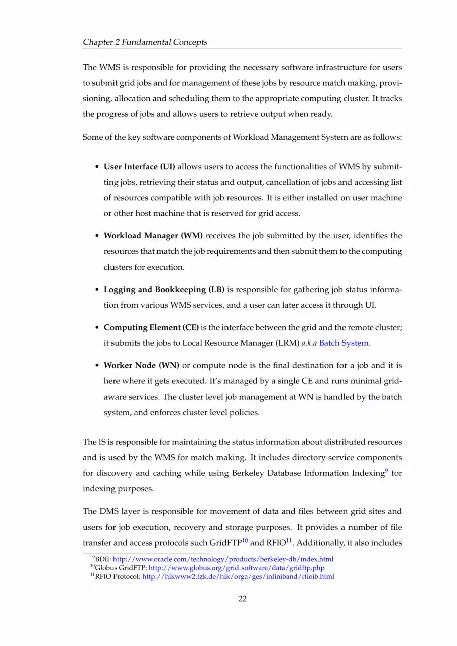
The WMS is responsible for providing the necessary software infrastructure for users
to submit grid jobs and for management of these jobs by resource match making, provi-
sioning, allocation and scheduling them to the appropriate computing cluster. It tracks
the progress of jobs and allows users to retrieve output when ready.
Some of the key software components of Workload Management System are as follows:
• User Interface (UI) allows users to access the functionalities of WMS by submit-
ting jobs, retrieving their status and output, cancellation of jobs and accessing list
of resources compatible with job resources. It is either installed on user machine
or other host machine that is reserved for grid access.
• Workload Manager (WM) receives the job submitted by the user, identifies the
resources that match the job requirements and then submit them to the computing
clusters for execution.
• Logging and Bookkeeping (LB) is responsible for gathering job status informa-
tion from various WMS services, and a user can later access it through UI.
• Computing Element (CE) is the interface between the grid and the remote cluster;
it submits the jobs to Local Resource Manager (LRM) a.k.a Batch System.
• Worker Node (WN) or compute node is the final destination for a job and it is
here where it gets executed. It’s managed by a single CE and runs minimal grid-
aware services. The cluster level job management at WN is handled by the batch
system, and enforces cluster level policies.
The IS is responsible for maintaining the status information about distributed resources
and is used by the WMS for match making. It includes directory service components
for discovery and caching while using Berkeley Database Information Indexing9 for
indexing purposes.
The DMS layer is responsible for movement of data and files between grid sites and
users for job execution, recovery and storage purposes. It provides a number of file
transfer and access protocols such GridFTP10 and RFIO11. Additionally, it also includes
9BDII: http://www.oracle.com/technology/products/berkeley-db/index.html10Globus GridFTP: http://www.globus.org/grid software/data/gridftp.php11RFIO Protocol: http://hikwww2.fzk.de/hik/orga/ges/infiniband/rfioib.html
22

Chapter 2 Fundamental Concepts
replication and catalogues services to speed up the process of the data transfer and
caching.
One key aspect of grid architecture is to provide sophisticated access control as dis-
cussed earlier in section 2.2.1. All the users and their related credentials linked to
their respective Virtual Organization are managed and controlled by AAA services,
and keeps tracks of resource usage on per user basis at each VO level to enforce re-
source sharing regime defined by the site and grid providers.
To enable grid managers and operators to run the system smoothly and efficiently, and
to troubleshoot whenever problems occur requires access to consistent and up-to-date
information so that problems can be quickly identified, analyzed and fixed. Manage-
ment System (MS) is responsible for maintaining grid services status, resource usage
and custom information related to running jobs for user access.
User
User Interfacejob submission
andmonitoring Information
System
resourcestatus
job and output
Job Queues
WorkloadManager
MatchMaking
Loggingand
Bookkeeping
Workload Management
System
StorageElementComputing Element
datatransfers
Batch System (LRM)
WorkerNode
WorkerNode
WorkerNode
Authentication, Authorization
andAccounting
datatransfers
jobsubmission
verification
FIGURE 2.5: Distribution and layout of the major components of the gLite middlwareservices.
23

Chapter 2 Fundamental Concepts
2.2.3 ATLAS Computing
ATLAS is one of the LHC experiments (see appendix B) and it’s workloads run on the
LCG grid. ATLAS users are part of the ATLAS virtual organization. To provide a uni-
form and comprehensive access to WMS infrastructure, ATLAS scientists have devel-
oped a high level computing software layer [37] that interacts with the grid middleware
and manages job submission, monitoring, resubmission in case of failures, queue man-
agement with different scientific grids such as Open Science Grid12, NorduGrid13 and
LCG while providing a single and coherent grid accesibility interface to its users.
2.2.3.1 Job Submission Mechanisms
The ATLAS computing software uses two different job submission mechanisms to the
grid:
1. Direct submission
In this model, the ATLAS users submit their jobs directly to a specific grid work-
load management system, which schedules the job to a suitable site that meets
job’s resource and software requirements. There are multiple application do-
mains from other experiments sharing the same grid infrastructure which leads
to latencies in scheduling the job and larger queue waiting times. If the job fails
while executing or gets terminated while waiting in the queue, then the user has
to resubmit their job. This leads to lower utilization rate of the system and higher
management overhead for the user.
2. Pilot Jobs
In recent years, ATLAS computing has developed a job submission framework
that interfaces with different scientific grids and takes care of job submission and
monitoring in an automated fashion. The system submits redundant and dummy
jobs called pilot jobs acquiring processing resources on the grid which are later
scheduled for real jobs by the external brokerage systems. Then the job is down-
loaded for execution from high-level ATLAS computing queues which is external
from the grid infrastructure.
12Open Science Grid: http://www.opensciencegrid.org/13NorduGrid: http://www.nordugrid.org/
24

Chapter 2 Fundamental Concepts
Pilot jobs are a kind of resource leasing mechanism, and their allocation and ac-
cess to the worker nodes is determined by the VO policies. They are responsible
for delegating the job scheduling responsibility away from the workload manage-
ment systems for resource provisioning and allocation for ATLAS jobs to reduce
unnecessary system load on the WMS. To prevent pilot jobs for submitting too
many jobs to local schedulers and reducing the share of resources for local jobs,
there are separate queue for pilot jobs and local jobs. This way a site administrator
manages the fair allocation of available job slots for pilot and local jobs.
Pilot jobs provides a very neat solution to over-come the unnecessary delays at
the WMS level, but there are certain limitation to their performance. One of the
main limitation is that a pilot job will have not control over what kind of job slot
it gets allocated by the local batch scheduler, and it only discovers the concrete
resource allocation once its deployed. At that stage, if the job slot doesn’t meet
the resource requirements of the downloaded job then the job is terminated, and
rescheduled. This could potentially lead to additional queueing delays.
ATLAS computing uses Production And Distributed Analysis system (PanDA)
for pilot job submissions [16], see section 5.1.1. Similar high level workload man-
agement and automated pilot systems are developed by other projects such as
Distributed Infrastructure with Remote Agent Control (DIRAC) [38].
2.2.4 Job Scheduling
With the evolution of grid middleware and development of pilot jobs, it’s important
to note that job scheduling takes place at different levels in the grid infrastructure.
Resource provisioning and allocation is handled by multiple and distributed system
which overlay each other. Three key systems that contribute to scheduling of ATLAS
jobs are following:
1. Central Scheduling: Jobs directly submitted to the grid are scheduled at the level
of WMS including pilot jobs to eventually acquire an execution slot at the worker
node. Scheduling at this level is determined by resource sharing policies between
various virtual organizations, and WMS makes sure that only jobs from authen-
ticated and authorized users goes through it.
25

Chapter 2 Fundamental Concepts
2. External Scheduling: Pilot job frameworks are external to the grid WMS and
once their jobs have acquired processing job slots, based on the configuration of
the job slot; pilot server sends the jobs from their centrally managed queues to the
worker nodes directly for execution. The primary metrics for scheduling at this
level is that the target worker node meets the software requirements of the job.
It is determined by the pilot job daemon when it starts executing on the worker
node, and send the details of resources it acquired back to PanDA server so that
job matching the acquired resources are sent to it.
3. Local Scheduling: Batch system level scheduling is the last link in the scheduling
hierarchy. They interface with grid CE which upon job arrival schedules them
to the worker nodes which could be either user jobs or pilot jobs. At this level
scheduling is more concerned with enforcement of local site policies such as sep-
arate queues for short, medium and long duration jobs.
2.2.5 Grid Sites Constraints
In this section, the existing problems faced by the grid sites (clusters participating in the
grid), especially those which are part of ATLAS experiment, are discussed. It provides
one of the core motivations to integrate virtualization in to the grid and utilize it’s
benefits to deploy and migrate portable execution environment i.e. virtual machines.
Following are the major issues that concerns such grid sites:
• Site Configuration: Whenever new middleware patches are released for the grid
sites, a number of sites get mis-configured resulting in the site going offline. This
results in no jobs being submitted to the site for a certain period of time until a
system administrator corrects the problem. This causes under-utilization of re-
sources and unnecessary administrative overhead for the site administrators.
• Platform Availability: Presently ATLAS recommends Scientific Linux CERN op-
erating system, which is derived from Red Hat Enterprise Linux with CERN spe-
cific modification, for its grid sites. This reduces choice for site providers who
might have a different OS preference due to local site needs and requirements
such as if the cluster is deployed in an academic institution and used for local
research activities.
26

Chapter 2 Fundamental Concepts
• Analysis Software: Atlas job requires additional stack of analysis software which
is 7GB in size. To support the grid sites, which do not have their own local
installation, CERN provides this software through read-only Andrew File Sys-
tem (AFS) over the Internet. Under heavy load, this leads to higher latencies,
which results in frequent job failures and could be very costly in terms of job
re-submission overhead for the long running jobs which have to be started again.
• Software Update: The update cycle for the ATLAS analysis software is around 2
weeks and requires downloading of hundreds of tarballs to the site. This process
is repetitive and burdensome for both the site providers and the ATLAS software
managers as it is prone to misconfigurations, and require efforts directed at trou-
bleshooting mis-configured sites.
Executing ATLAS jobs in virtual machines will certainly enable the site administrators
to manage their physicals resources more efficiently as operating system virtualiza-
tion decouples the execution environment from the host machines by turning them
into generic compute resources. Further more, pre-configured and pre-certified virtual
machine images with ATLAS software, if available locally at the site, will provide an
elegant solution to the current deployment strategy that relies on error prone software
distribution and update life cycle. There has been some progress on this front where
large grid sites participating in CERN’s LCG have developed regular virtual machine
images used for job execution. It will also open an avenue in the future that user’s
could package their job with the required software in the virtual machine image and
send it to the grid for execution.
27

Chapter 2 Fundamental Concepts
2.3 Summary
This chapter has described the fundamental concepts needed by reader that runs through
out this thesis, and placed the research into context. It provides a detailed discussion of
virtualization technology and the resultant overhead which arises as hypervisor soft-
ware has to continuously handle interrupts and kernel calls coming from guest operat-
ing systems.
It gave an overview of different technologies such as para-virtualization, emulation,
container and binary translation to achieve operating system virtualization at the soft-
ware level. It also described the hardware based virtualization which is increasingly
used these days due to fact that microprocessor manufacturers have updated the pro-
cessor hardware architecture by removing or adapting the CPU instructions to enable
more transparent virtualization of the guest OS.
In later sections, a detailed overview of the grid technologies, its goals and architecture
has been presented. This was further expanded in the context of a real-world grid
middleware i.e. gLite which has been deployed on the WLCG grid for CERN’s flagship
LHC experiment. Various components of gLite middleware has been presented such
as workload management system, accounting and book keeping, user-interface and
computing nodes, and their relationship to each other. This provided the basis for the
reader to fully locate the ATLAS experiment and it’s PanDA pilot job framework in
the context of grid computing. This was important since both ATLAS jobs and PanDA
pilot framework has been the subject of research in this thesis as real-world case study.
Finally, this chapter concluded with a discussion about the scheduling of jobs that has
taken place at various levels within grid workload management system, at batch sys-
tem level and finally by the PanDA pilot server. It also highlighted the challenges faced
by both system administrators and grid users in managing and using such a large and
distributed infrastructure. Operating system level virtualization is one of the promis-
ing approaches that could help in resolving some of these challenges to enable scientific
grids to be more dynamic, agile and optimal in delivery of computational services to
scientists around the globe.
28

Chapter 3
Literature Review
“We are made wise not by the recollection of our past, but by the responsibility for our future.”
George Bernard Shaw
According to Ruth et al. ”Grid computing technology....provides opportunities for a broad
spectrum of distributed and parallel computing applications to take advantage of the massive
aggregate computational power available...spanning multiple domains” [39].
Large scale distributed infrastructures such as grid and PlanetLab1 serve the needs of
diverse set of users running very many different applications. Some of these applica-
tions require pre-configured and customized execution environments (e.g. a particular
OS with specific libraries needed for diverse set of workloads). It may not be possible
to fulfill all such requirements in a grid infrastructure all the time for every worker
node. This requires the underlying infrastructure to possess certain flexibility to meet
competing and often contrasting requirements. Virtualization is a promising technol-
ogy to provide such flexibility to configure and deploy on-demand virtual execution
environment in a distributed grid infrastructure.
This chapter presents an overview of the body of work done to integrate virtualization
in to large scale grid infrastructures and attempts to categories different techniques.
Some of these techniques interfaces with batch systems to integrate virtualization at
1PlanetLab overlaying Infrastructure. See http://www.planet-lab.org
29

Chapter 3 Literature Review
the gird site level or solely focus on virtualizing a local cluster, while others directly in-
tegrate with grid middleware software. These techniques are discussed in detail along-
side with their architectural differences and implementation methods (see section 3.1).
This provides a comparative overview of the techniques that are complementary to the
approach taken to virtualize LCG grid through PanDA pilot (see chapter 5).
Yet, there is a parallel phenomenon going on in the large scale distributed computing
community to enable pay as go access to the infrastructure namely cloud computing.
Although the research presented in this thesis is primarily targeting grid computing,
but to properly contextualize this work and to provide an over view of the emerging
trends, a discussion on cloud computing is included in this chapter as well (see section
3.1.2).
Virtualization technology incurs a performance penalty as discussed in previous chap-
ter. A detailed analysis of it’s impact on job performance is further discussed in section
3.2.1 along side optimization techniques to overcome and reduce the impact of over-
head. This is relevant to the scope of this thesis since one of its main objective is to
investigate optimization techniques that are complementary to job schedulers by lever-
aging the overhead profile which changes due to the types of workload running in
virtual machines.
Section 3.3 describes live migration of virtual machines, and power management to
optimize infrastructure management with emphasis on security implications of virtu-
alization. Live migration techniques are useful to reduce virtual machine downtime
and migration times. Power management via intelligent task placement and determin-
ing hotspots in the cluster is crucial to minimize the energy costs of a data center, and
various approaches taken by other researchers are summarized. Although these topics
are beyond the scope of this study but are included since they are relevant to the issues
arising when grid infrastructure is virtualized.
Finally, a discussion of work related to various scheduling approaches taken to opti-
mally schedule virtual machines for interactive and batch applications is presented.
Scheduling architecture of the underlying Xen hypervisor provides number of differ-
ent scheduling algorithms and parameters to tweak job performance, and is presented
in section 3.4, and appropriate references are made to the contribution of this thesis
presented in next few chapters.
30

Chapter 3 Literature Review
3.1 Virtualization in the Infrastructure
The primary motivations for the uptake of virtualization has been resource isolation,
capacity management and resource customization: isolation and capacity management
allow resource providers to isolate users from the grid site and control their resource
usage while customization allows fine-grain modification of the execution environment
without affecting the host system.
Various approaches have been taken to integrate virtualization in grid infrastructure,
and they are discussed in the following section.
3.1.1 Virtualized Grid Computing
3.1.1.1 Resource Management
Deploying grid jobs in VM’s on-demand does not only involve performance and man-
agement issues but also presents challenges such as how to provision and allocate re-
sources for job submission, suspension and migration. This could be described as Qual-
ity of Life regarding an execution environment meeting all software requirements and
Quality of Service in relation to resource allocation [40]. Before looking in to various
techniques about how to virtualize grids and clusters, it’s important to define particu-
lar machine resources required for these techniques.
Resource Definition
The resources that have to be provisioned for a virtual machine before it could be de-
ployed are as follows:
• VM Image: The VM images contain the guest operating system and must be
downloaded to the destination machine before it can start. This requires allo-
cation of disk space on the storage system. VM image could be mounted as a
31

Chapter 3 Literature Review
loopback device2 with additional disk space for data write or it could be decom-
pressed into a logical volume group (LVM) which also facilitates to take periodic
snapshots of the disk if needed.
• Memory: Just like any other machine, VM’s require access to Random Access
Memory (RAM) which generally has to be pre-allocated. For multiple VM de-
ployment, RAM have to be reserved for each VM. Size and availability of RAM
on a given machine constrains how many VMs can be deployed simultaneously.
• Networking: Network bandwidth is another important resource for download-
ing VM images and input data sets for jobs on destination machines. Under a de-
fault configuration, network bandwidth consumes CPU shares of the VM while
the network bridge3 is emulated by the hypervisor (VMM) which requires man-
agement of network traffic in hypervisor software layer.
• CPU: The CPU share among all the virtual machines is allocated by the hypervi-
sor and is configurable for different VMs. These days multi-core CPU’s are widely
deployed and could dramatically influence a site provider’s virtual machine de-
ployment model; pre-deployed (pool of VM already running grid services) vs.
on-demand.
Provisioning Model
Resource management and efficient provisioning poses complex algorithmic challenges.
Each resource request is driven by multiple factors such as how much of the resource is
required, when it is required, how long it is required for and where it could be allocated
in the system. Grit et al. [41] have defined it as a knapsack problem where different items
and values have to be fitted in finite space of fixed volume. It becomes a multiple knap-
sack problem with multiple sites or physical hosts with different resource capabilities
such as CPU, disk, memory and network bandwidth.
Nevertheless, the resource-provisioning model will also depend on how virtual ma-
chines are deployed. There are two ways to achieve this:
2In Unix-like operating systems, a loop device, vnd (vnode disk), or lofi (loopback file interface) is apseudo-device that makes a file accessible as a block device.
3A software layer that connects the underlying networking interface hardware to the virtual machine.
32

Chapter 3 Literature Review
• On-Demand (no predeploy): For each new job request, a new VM is deployed
using an image that has the complete software environment required by the job.
Since deployment of VM from scratch takes a constant time; if its greater than the
job duration then this model will be least efficient as the job will be most likely to
miss its deadline.
• Sliver Resizing (predeploy): In this scenario, a pool of virtual machines are pre-
deployed and running on a cluster. Upon job arrival, the physical resources (CPU,
disk, network, memory) for the virtual machine are dynamically adjusted. This
model improves avg. job turnaround - time it takes for a job to complete, for short
duration jobs. The constraints of this approach is that a pre-defined set of VM
images are used which would match most of job requirements but not all of them.
This could be realistic when a site provider only participates in a single Virtual
Organization (VO) and have to manage limited set of pre-defined VM images.
For a site with multiple VO participation, there could be large set of VM images
and pre-deploying them may not be practical for all real-world use cases.
VM Image Management
Virtual machine image management poses serious challenges to large-scale deploy-
ment of virtualization in the grid. It’s a difficult problem to address and raises ques-
tions about how to create, certify and propagate these images to the required destina-
tion machines when required. The virtual machine startup, shutdown and destruction
stay constant as of 23 seconds, 11 second and <1 sec respectively for the VM image of
size of 2GB-4GB when benchmarked on 3GHz CPU [42]. The largest overhead in the
virtual machine deployment is due to image staging to the computational node and it
significantly increases job turnaround time.
Bradshaw et al. [43] have identified the following issues related to VM image manage-
ment:
• Generation: The flexibility to customize virtual machine images to meet job re-
quirements on-demand requires that images to be generated on-demand or prior
to deployment depending on a specific configuration such as user rights, applica-
tion installation and configuration etc. Configuration management process needs
33

Chapter 3 Literature Review
to be automated to specify which packages have to be included in an image.
Generating images on-demand, depending on the configuration, constitutes to
a significant time overhead. This could be avoided by decoupling the process
of image generation from the job request so that they could be generated, config-
ured and certified by the site administrators in advance. Such a configuration and
customization process is also referred as Contextualization [44], and the resulting
virtual machine is called Virtual Appliance [45].
• Management: Over the lifetime of an image, which is generally of few weeks,
a mechanism has to be developed to automate image updating process to patch
latest security packages. This requires some sort of a standard way to define
configuration, probably expressible in XML, so that distributed images are auto-
matically updated when new patches are available.
• Propagation: Another challenge is about devising a policy of where to locate
the images (on remote gird sites or locally cached on each cluster) and how to
download these images to worker nodes when needed. Relative locality (locating
images closer to where they are needed) reduces the time required for an image
to be downloaded to the destination machine but puts constraints on local sites
for having additional storage space since a typical ATLAS VM image is around
15 GB each. This also puts additional constraints on the network bandwidth and
could be optimized utilizing content based downloading mechanisms where only
the image difference is downloaded to the target machine, and patched to the VM
image on the fly [46].
There are also security risks associated with VM images as the site administrators
would be reluctant to execute images on their resources which they have not certi-
fied. Hence, allowing users to download their own customized virtual machine im-
ages, which offer maximum flexibility, poses a risk that a malicious grid user could
utilize such a VM to stage further attacks. One possible model could be virtual image
repository for each site containing images certified by the site authority whereas also
reducing image download overhead through relative locality.
Constandache et al. have employed a different approach to this challenge by developing
a technique to modify a generic VM image on the fly according to it’s user requirements
[47]. They used a control-binding protocol by using a pre-installed piece of software in
34

Chapter 3 Literature Review
the VM image which upon boot up first authenticates itself with its owner or a con-
troller proxy through secure tokens, and then customizes it according to its need. This
reduces the overhead of generating VM images on the fly which can rather be config-
ured on-the fly from a single VM image.
Recently, cloud software infrastructure providers have developed proprietary solutions
to address some of the challenges discussed above related to VM image management
and could be applied to grid computing on ad-hoc basis. Cloud computing infrastruc-
tures have developed standard ways to access distributed data (e.g. S3 query language
provided by Amazon Web Services), use of high-speed network based access for vir-
tual machine images and automatic patching of the virtual machine images when new
updates becomes available etcetera.
3.1.1.2 Deployment Techniques
There have been a number of approaches taken to bring in virtualization capabilities
in to clusters and grid systems. Often these techniques have employed methods that
are specific to a particular application domain e.g. serial jobs requires different sort of
mechanisms as compared to parallel job where job performance depends on message
passing, thus has to be deployed together in close proximity to reduce latency in mes-
sage passing which leads to higher synchronization costs. Also, significant work has
been done in the context of deployment platforms already in production use, and there-
fore makes sense to modify them to enable virtualization. This is the same approach
taken for the research work presented in this thesis.
These deployment techniques could be broadly grouped as follows:
• Virtual Cluster Management (VCM): In this model, no modifications are made
to the Cluster or Local Resource Managers (LRM) (a.k.a. batch systems) architec-
ture. The implementation of virtualization is completely external and opaque to
35

Chapter 3 Literature Review
the batch system e.g. Condor4, Torque5 and Platform LSF6. All the issues of re-
source allocation, scheduling, resource provisioning, security and optimization
are handled by an external software layer through an overlaying management in-
terface with batch systems and grids, but primarily work independently to pro-
vide clusters on-demand.
• Virtual Grid Coordinator (VGC):
In this model, VGC is implemented to interface with the existing grid workload
management system such as WMS or Globus Grid Resource Allocation and Man-
agement (GRAM) service. Grid job scheduling is done independent of the under-
lying virtualization management system, and VGC takes care of resource provi-
sioning, allocation and scheduling of the virtual machines as job arrives at a local
site for execution.
• Virtual Batch System (VBS):
This model follows the approach of integrating virtualization within the batch
system which stays transparent to the external grid infrastructures and utilize its
capabilities. In this model, the pre-existing schedulers would have to be modified
to incorporate virtual machine states corresponding to job states such as running,
paused or cancelled in order to monitor both jobs and virtual machines. This
enables the batch system for on-demand deployment and periodic resizing of
virtual machines according to the system load.
Virtual Cluster Management
The Cluster-On-Demand (COD) project falls under this category and implemented a
service-oriented architecture [48]. COD implements resource allocation based on CPU
speed, memory and disk allocation within the isolated virtual cluster. It can manage
both physical and virtual clusters where some of the machines are physical while oth-
ers are VM’s. Its extensible architecture allows specific modules to be plugged-in to
4Condor project for High Throughput Computing (HTC). See http://www.cs.wisc.edu/condor/5PBS/TORQUE is an open source resource manager providing control over batch jobs and distributed
compute nodes. See http://www.clusterresources.com/products/torque-resource-manager.php6Platform LSF is the workload management solution for high performance computing (HPC) environ-
ments, schedules batch and interactive workload for compute- and data-intensive applications in clus-ter and grid environments. See http://www.platform.com/workload-management/high-performance-computing
36

Chapter 3 Literature Review
provide fine-grained services, and it could interface with grid web-services for cluster
management and resource brokering.
They also introduce a concept of lease which is based on weak assurance, or best effort,
and represents a contract of a resource and is part of their Shirako project to handle site
based policy management and resources leasing [49]. It doesn’t implement advance
reservation of resources and the model is implemented in such a way that fundamen-
tals of leasing mechanism are decoupled from the leasing policy which varies from site
to site. Thus allowing fine-grained control over resources under different deployment
scenarios; it could be storage, network, and physical or virtual clusters.
Shariko can provide simpler resource allocation policies with in a site, which are exten-
sible, but more complex economic policies with external sites using credits are achiev-
able with an additional software module called Cereus [50]. The COD implementation
could be best described as distributed overlaying cluster management system, which
is fairly flexible and extensible, but it lacks precise mechanisms for integration in to
EGEE, OSG or other grids.
On the other hand, Maestro-VC project has taken a different implementation route than
COD. COD primarily focused on fine-grained resource allocation for both physical and
virtual machines, Maestro-VC tries to completely virtualize a physical cluster, and then
creates virtual clusters on-demand for its clients [51]. Their resource allocation model
is different since it is concerned more with VM performance which executes a par-
ticular job. Maestro-VC could be described as virtual batch system where it runs its
own management software on the physical machines along side with a global and local
scheduler to orchestrate virtual clusters on-demand.
This is particularly useful for parallel jobs that have to be run simultaneously and with
in a close-proximity to reduce latency for message passing, and Maestro-VC attempts
to address this problem by co-locating virtual machines on physical macines. Such a
deployment tool could be integrated in to the grid by the site providers to increase
resource utilization, but it remains confined to small scale cluster deployment rather
then large scale virtualization in the grid.
37

Chapter 3 Literature Review
Virtual Grid Coordinator
Virtual grid coordinator (VGC) differs from the previous technique as it is more focused
on integrating with the grid middle ware then fine-grained resource management at the
cluster level. It could be used in conjunction with the VCM tools.
Virtual Workspaces [52] (VW) project is a part of Globus Middleware7 and has been
very tightly integrated into its services. It defines a virtual machine instance as a
workspace.
Whenever a new job arrives, VW service manager initiates a workspace deployment
process. After verifying resource availability and job requirements on the target node,
a workspace creation request is communicated to the VW Node Manager that deploys
the virtual machine on the physical node which is very similar to vGrid agent as dis-
cussed in section 5.1.2.1. The virtual image is either taken from the local cache if present
or else downloaded from the central repository. Once VM is deployed, VW Server is
notified and it updates its resource status, and Grid file transfer protocol (FTP) service
is used for any pre-staging data/file transfers into the virtual machine for each job ex-
ecution. Upon job completion, VW Node Manager terminates the virtual machine with
the similar architectural approach as we implemented for PanDA daemon (see section
5.1.2.3).
VW has also developed techniques for image downloading and caching to the target
physical nodes. Despite the promising results from their prototypes, Virtual Workspaces
project kept its focus on integration and deployment of virtual execution environments
in the Globus middleware, in particular, and yet much has to be done to achieve opti-
mization in resource allocation and scheduling of virtual machines.
In comparison to VW, GridWay [53] is a meta-scheduling system that allows unat-
tended execution of grid jobs by supporting all the steps involved in the life-cycle of
a job such as resource discovery and selection, job preparation, submission, monitor-
ing, migration and termination. It could be used as VGC for gLite middleware while
7Globus Grid Alliance. See http://www.globus.org
38
Chapter 3 Literature Review
using VW as a virtual machine deployment backend at the cluster level. Their proof-
of-concept deployment has been for PBS/Torque batch system using XMM-Newton8
scientific application which matches ATLAS workloads in many respects.
One if its component is Execution Manager that interfaces with GRAM grid web-service
and submits a wrapper program to it. The wrapper program validates availability of
a virtual machine matching job requirement, and if none is available invokes virtual
workspaces to deploy a virtual machine. While the virtual machine is deployed, it polls
for virtual machine boot up. Once the virtual machine is deployed, then PBS/Torque
prolog step, executed before job is started, is initiated to copy input files into the virtual
machine. Upon the completion of the job, the wrapper program terminates the virtual
workspace initiated by epilog step - always executed at the end of each job.
This combination of VW and GridWay is very similar to the implementation taken for
Virtual PanDA pilot. The major difference is that VW-GridWay combination solely em-
ployed Globus grid resources, and makes it harder to be integrated in to gLite middle-
ware which uses PanDA pilot job framework. Secondly, it supports more generic jobs
which comes in with small and pre-package payload rather than the existing PanDA
pilot jobs which downloads its preload between VM setup and execution to avoid net-
work overhead of virtualization.
Virtual Batch System
Virtual batch system (VBS) approach is similar to VCM as it also focuses on the local-
cluster but rather then directly managing the cluster, it enhances the capabilities of
the batch system. Thus utilizing scheduling, resource allocation, queue management
and other features provided by the batch systems. VBS could complement some of
the capabilities of the VCG approach where former provides virtualization enablement
and latter provides integration into the grid.
Magrathea have one of the most interesting approaches in enabling virtualization in
the batch system [54]. Their model is based on a paradigm shift of scheduling virtual
8The European Space Agency’s (ESA) X-ray Multi-Mirror Mission (XMM-Newton) is a spacebased telescope. It carries 3 high throughput X-ray telescopes with an unprecedented effec-tive area, and an optical monitor, the first flown on a X-ray observatory. The large collectingarea and ability to make long uninterrupted exposures provide highly sensitive observations. Seehttp://xmm.esac.esa.int/external/xmm about/
39

Chapter 3 Literature Review
machines rather than jobs in the context of deployment by integrating their services into
the batch system to seemless scale up and down of pre-deployed pool of virtualized
worker nodes. It has extended PBS Professional9 scheduler to include virtual machine
states as jobs starts, executes and finishes.
The architecture of Magrathea consists of a master daemon and slave daemon. A mas-
ter daemon runs on each computational/worker node in a supervisory virtual machine.
It is responsible for monitoring worker virtual machine states and allocating resources
to them on demand. Each worker virtual machine runs slave daemon that intercepts
job requests from the scheduler for execution and if it does, then it communicates its
status to the master daemon running on the worker node.
If a job is interrupted or suspended during execution, then slave daemon notifies the
master daemon, which updates the virtual machine state in the cache status interfacing
the scheduler so that scheduler could reallocate resources using sliver resizing technique
to dynamically scale up or down physical resources allocated to a given VM. In such
an event, the master daemon will reduce virtual machine resources such as CPU share,
memory and will put the virtual machine in hibernation mode. For dynamic resource
allocation, master daemon interfaces with the Xen hypervisor on each worker node. Job
preparation and monitoring is handled by PBS monitoring facilities using standard PBS
epilog/prolog scripts that are always launched at the start and end of the job execution.
Currently, Magratheas usage scenario is one job per active virtual machine, and it is a
static deployment model where VM’s are pre-deployed and pre-configured as worker
nodes. It has been deployed for EGEE infrastructure where ATLAS jobs also get exe-
cuted. Another constraint to their approach is the lack of an image management sys-
tem, which would be critical, to manage images in a central repository with a local
cache to deal with a large-scale virtual machine deployment.
On the other hand, the Dynamic Virtual Clustering project have a taken a different ap-
proach of deploying virtual clusters on per job basis [55]. Its prototype implementation
9Portable Batch System (or simply PBS) is the name of computer software that performs job schedul-ing. Its primary task is to allocate computational tasks, i.e., batch jobs, among the available computingresources. It is often used in conjunction with UNIX cluster environments. PBS is supported as a jobscheduler mechanism by several meta schedulers including Moab by Cluster Resources and GRAM (GridResource Allocation Manager), a component of the Globus Toolkit. See http://www.pbsworks.com/
40

Chapter 3 Literature Review
is using Xen hypervisor, Moab Scheduler10 and Torque resource management system.
It analyses parallel and message passing interface (MPI) HPC workloads where parallel
VM’s are deployed on demand to executed all parallel jobs in one go that depend on
each other to execute successfully. DVC focuses on three objectives to achieve this:
1. To run a job on a cluster without modifying the underlying physical resources.
Upon arrival of an MPI job, a cluster of virtual nodes running resource manager
daemon is deployed. The resource manager daemon takes care of the staging of
files, job monitoring and notifying Moab scheduler upon job termination.
2. To migrate jobs with in the cluster. If a job has to be suspended and later on
moved to another virtual cluster due to heavy load or else, then DVC deploys the
job on another cluster while keeping the previous job image to keep the environ-
ment consistent. This way it increases job capacity by utilizing all the available
resources and reduces average job turnaround time.
3. To achieve cluster spanning when additional resources for a job are required. The
cluster scheduler borrows additional resources from another cluster scheduler
for a given timeframe, and returns the resources upon the completion of the jobs
using leasing mechanisms as described earlier in VCM deployment model. Once
the job is terminated, then DVC shuts down virtual cluster and Moab scheduler
is updated for the availability of physical resources for future job requests.
DVC achieves virtual clustering by tightly interfacing with the batch system to provi-
sion, allocate and schedule VM resources for MPI jobs.
3.1.2 Rising ”Clouds”
What is Cloud computing? According to National Institute of Standards and Technol-
ogy (NIST) ”Cloud computing is a model for enabling ubiquitous, convenient, on-demand
network access to a shared pool of configurable computing resources (e.g., networks, servers,
storage, applications, and services) that can be rapidly provisioned and released with minimal
management effort or service provider interaction.” [56].10Moab Grid Suite is a powerful grid workload management solution that includes schedul-
ing, advanced policy management, and tools to control all components of grids. Seehttp://www.clusterresources.com/pages/products/moab-grid-suite.php
41
Chapter 3 Literature Review
This buzzword has clearly captured the imagination of researchers working in the do-
main of distributed, grid, utility and service-oriented computing [57, 58]. Can cloud
computing be described as ”utility computing with a marketing friendly name....sprinkled
with little internet pixie dust” or is it ”grid computing done right” as claimed by J. Barr
in his article [13].
Cloud computing is a flexible resource pool which is elastic to grow or shrink based on
demand fluctuations and focuses on better resource utilization and business flexibility
to scale up and down the capacity while leveraging technologies such as virtualization
with standard interfaces to access the infrastructure. Where as, grids are a set of re-
source pool (servers, disks, tape drives, network resources) reserved and provisioned
for each virtual organization to enhance resource sharing among complex scientific ap-
plications, and often requiring dedicated infrastructure to maximize highest possible
performance and task throughput. These comparison are shown in table 3.1. Buyya et
al. have provided a very detailed analysis of clusters, grids and cloud paradigms and
the need to converge them in the 21st century computing vision [59].
There are currently various approaches to deploy clouds from federating clusters to
desktop grids and data centers. Some even have explored the idea of transforming en-
terprise desktops into a cloud and delivering desktop computing over cloud by bench-
marking capacity planning and workload analysis in the context of an enterprise [60].
While others have ventured on evaluating cost benefits of Volunteer Computing (VC)
such as BOINC project11 in the context of running parallel and compute-intensive ap-
plication both on clouds and volunteer computing [61]. Their results currently shows
lower start-up and operating costs using VC platform as compared to cloud utilization
when utilization is extrapolated for a year long commitment.
Nevertheless, due to the large number of cloud infrastructure providers in industry
with different services, the distinction between them has been obfuscated leading to
confusion among researchers and engineers to fully utilize the capabilities of the cloud
services for their particular applications. Lenk et al. have come up with an architectural
model that categories existing cloud services into various service types [62]. According
to them, the stack consists of three major categories:
11BOINC Project: Open-Source software for volunteer computing and grid computing. Seehttp://boinc.berkeley.edu/
42
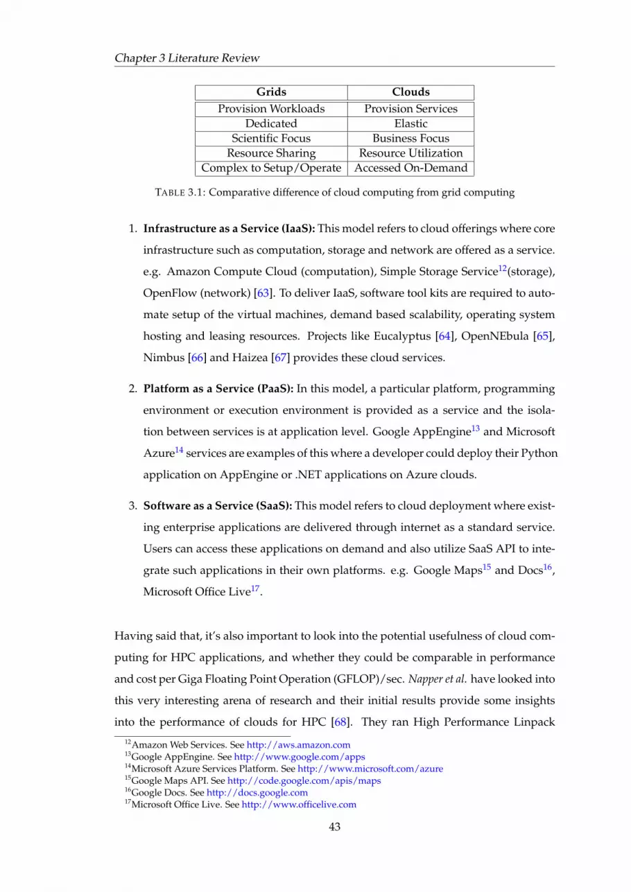
Chapter 3 Literature Review
Grids CloudsProvision Workloads Provision Services
Dedicated ElasticScientific Focus Business Focus
Resource Sharing Resource UtilizationComplex to Setup/Operate Accessed On-Demand
TABLE 3.1: Comparative difference of cloud computing from grid computing
1. Infrastructure as a Service (IaaS): This model refers to cloud offerings where core
infrastructure such as computation, storage and network are offered as a service.
e.g. Amazon Compute Cloud (computation), Simple Storage Service12(storage),
OpenFlow (network) [63]. To deliver IaaS, software tool kits are required to auto-
mate setup of the virtual machines, demand based scalability, operating system
hosting and leasing resources. Projects like Eucalyptus [64], OpenNEbula [65],
Nimbus [66] and Haizea [67] provides these cloud services.
2. Platform as a Service (PaaS): In this model, a particular platform, programming
environment or execution environment is provided as a service and the isola-
tion between services is at application level. Google AppEngine13 and Microsoft
Azure14 services are examples of this where a developer could deploy their Python
application on AppEngine or .NET applications on Azure clouds.
3. Software as a Service (SaaS): This model refers to cloud deployment where exist-
ing enterprise applications are delivered through internet as a standard service.
Users can access these applications on demand and also utilize SaaS API to inte-
grate such applications in their own platforms. e.g. Google Maps15 and Docs16,
Microsoft Office Live17.
Having said that, it’s also important to look into the potential usefulness of cloud com-
puting for HPC applications, and whether they could be comparable in performance
and cost per Giga Floating Point Operation (GFLOP)/sec. Napper et al. have looked into
this very interesting arena of research and their initial results provide some insights
into the performance of clouds for HPC [68]. They ran High Performance Linpack
12Amazon Web Services. See http://aws.amazon.com13Google AppEngine. See http://www.google.com/apps14Microsoft Azure Services Platform. See http://www.microsoft.com/azure15Google Maps API. See http://code.google.com/apis/maps16Google Docs. See http://docs.google.com17Microsoft Office Live. See http://www.officelive.com
43

Chapter 3 Literature Review
(HPL)18 to benchmark the performance of dense linear algebra in Amazon EC2 Cloud.
Their results show that performance drop was exponential when linearly increasing the
problem size and available cluster size to match the problem, and they could only ob-
serve 70% of peak theoretical computational performance for a single node size cluster.
They identified that lack of large available memory and faster network interconnects
as potential performance bottlenecks in the cloud.
Another issue related to cloud based model is security of the data within the cloud.
This could be of two types; first that cloud provider respects the integrity of the data
of their customers by not not introspecting the VMs, and secondly whether a malicious
user can break into one’s VM through co-residency placement. Co-residency placement
refers to multiple VM’s sharing the same physical infrastructure. Cloud providers use
load-balancing algorithms to distribute the VM’s for a particular user with in a cluster
of physical machine, and these VM’s have both internal and public IP address. Fur-
thermore, this increases the likelihood of an adversary sharing the same computation
machine as a target customer, and perhaps able to interfere with the integrity of the
target customer through cross-VM attacks.
Ristenpart et al. have successfully shown in their study that such attacks are not only
possible but feasible to develop [69]. They employed various techniques first to deter-
mine co-residency and then to launch an attack on a target VM (which in this case is
their own). Using network probing, IP address translation and DNS queries, measur-
ing small packet round trip times, establishing covert-disk channels through random
read/write of 0/1 bits and shared memory. They were first able to create a map of exe-
cuting VMs in the cloud and then later co-place their ”attacker” VM next to the ”target”
with the success rate of 40%. This study is very valuable in the context of security of
utilization in the cloud, and raises important questions about their viability for HPC
applications with the current state of technology.
Nevertheless, there are high level tools emerging to rapidly deploying a cluster on a
cloud. One such project is SnowFlock that uses VM cloning from a pre-defined image
and deploys it on the cloud with a a cluster size ranging from up to ten’s of nodes
[70]. It significantly reduces adaptation and entry barrier for the HPC applications to
18HPL is a software package that solves a (random) dense linear system in double precision (64bits) arithmetic on distributed-memory computers. It can thus be regarded as a portable as wellas freely available implementation of the High Performance Computing Linpack Benchmark. Seehttp://www.netlib.org/benchmark/hpl/
44

Chapter 3 Literature Review
be quickly deployed on the cloud infrastructure. Another example is the Gaia project
which deployed an data grid in the Amazon cloud to analyze data of five years of 2
million stars taken from number of international space telescopes where the primary
emphasis was to get a grid up and running with minimum investment in the physical
infrastructure [71].
W. Gentzsch argued ”Grids did not evolve in to the next fundamental IT infrastructure for
every thing and every body” [72]. The diversity of computing environments for differ-
ent scientific applications led to a usage model which is significantly different from
business usage where emphasis is on flexibility and less on performance. By combin-
ing grids with automation, virtualization, elastic capacity management leads to cloud
computing where both co-exit in their respective domains of utility.
Despite the advantages and flexibility of clouds, they also abstract away the visibility
of underlying platform which is often necessary for HPC applications where code is
pre-compiled for a particular platform to yield best performance. Possible examples of
is a genomic study of protein folding, climate change, analysis of physics data coming
from LHC at CERN. Unless and until new paradigms and programming languages are
developed which allow performance optimization with out the knowledge of target
platform, grid computing will continue to serve as primary computational model for
HPC community. Additionally, whenever more computational capacity is required for
a short span of time, cloud computing would be able to provide such capacity without
long term commitments and on-demand basis.
45
Chapter 3 Literature Review
3.2 Virtualization and Performance Challenges
There are several ways to build a system to share machine resources among heteroge-
neous applications. The simplest way has been to run a host with a standard operating
system such as Linux or Windows, and running applications as user processes. In such
a model, OS multiplexes the underlying CPU, memory, disk and network resources
among competing applications. Such an approach also creates complex configura-
tion interaction between running applications, and administrative overhead to manage
such a system. Such an approach poses additional challenges to prevent one applica-
tion adversely affecting the performance of the concurrently running applications, and
have been subject of OS research in late 90’s. One way to address this problem was to
enable operating system to provide performance isolation at process level [73, 74].
Development of the virtualization hypervisor, which multiplexes the physical resources
at the granularity of entire operating system is able to provide better resource utiliza-
tion but at the cost of performance overhead. Since running a full OS is more heavy
weight than a process in terms of initialization and resource consumption. Successful
partitioning of a machine to execute concurrent operating system poses a significant
challenge of performance isolation among virtual machines ”especially when virtual ma-
chines are owned by mutually distrusting users” [75].
In section 2.1, the key design issues of virtualization are discussed in detail highlight-
ing performance overhead incurred due to constant interception of hardware events by
the hypervisor when ever guest OS tries to access machine resources. In this section,
additional disk and network (I/O) overheads are discussed and a survey of on-going
research is presented where various approaches have been taken to optimize virtual-
ization overhead in the context of HPC applications with in Xen hypervisor.
3.2.1 Overhead Diagnosis and Optimization
Virtual machines provide Fault Isolation so that failure in one virtual machine does not
affect other VMs hosted on the same machine, and Performance Isolation that the re-
source consumption of one VM should not compromise the promised guarantees to
the adjacent VM’s.
46

Chapter 3 Literature Review
Xen hypervisor inserts a logical isolation layer between the hardware and I/O device
drivers (disk, network etc) to achieve fault isolation. In the initial design of Xen, de-
vice driver code was part of the hypervisor and provided safe shared access. Since
external events in device drivers could potentially create issues of dependability, main-
tainability, and manageability with in the hypervisor code, Xen moved to the architec-
ture where device drivers were hosted in Isolated Device Domains (IDD) and executed
in a separate scheduled virtual machine called Domain0 / dom0 or Dom0 [76]. Dom0 is
created at boot time and provides the control interface to manage the VM’s and their
resource allocation policies.
This model is certainly more efficient to enable fault isolation but results in a more com-
plex CPU model. It has two aspects; CPU consumed by the guest VM, and CPU con-
sumed by the IDD in the Dom0 that contains the un-modified device driver and per-
forms I/O processing on the behalf of the requesting VM.
3.2.1.1 Diagnostic and Monitoring
Diagnostic and monitoring of the VM resource consumption requires an accurate mon-
itoring framework that not only reports the amount of CPU allocated by the scheduler
for the execution of a particular VM but also the work done for I/O processing in IDD
for that particular VM e.g. consider a guest VM limited to 25% CPU consumption. If
the I/O processing in IDD for this VM accounts for 15%, then that VM has actually
consumed 40% of CPU.
To accurately monitor resource consumption in each domain and in IDD for each do-
main, Gupta et al. developed a monitoring and performance profiling framework called
XenMon. It provides sub-tools to enable event-logging with in Xen hypervisor at ar-
bitrary control points to collect information, and then provide meaningful information
[77]. XenMon has been integrated into the official Xen 3.0 code base.
Cherkasova et al. built their work on it, and conducted investigations to accurately mon-
itor CPU consumption for a network intensive application i.e. a web server [78]. Since
Xen uses a technique called Page Flipping for the exchange of I/O data between the Xen
and guest VM, where the memory page containing the I/O data is exchanged with an
unused page provided by the guest VM.
47
Chapter 3 Literature Review
They ran their experiments where varying degree of webpage size (from 1KByte to 70
KByte) were requested from the web server in the VM, and measured the number of
memory pages exchanged between the hypervisor and Xen, and thus calculating CPU
processing time of Dom0.
They observed that smaller network requests i.e. < 5KB were CPU bound since a min-
imum number of memory pages must be exchanged for each KByte of TCP/IP data
and the server could only do a maximum number of exchange at a given clock-speed
of the processor. Larger network requests i.e. > 50KB were found to be network-bound
where bottleneck was the total available network bandwidth available to the system
and confirmed a prior study [79].
Menon et al. attempted to optimize I/O overhead by developing a system-wide per-
formance profiling toolkit called XenoProf [80]. Their approach is to identify micro-
architectural components such as the cache and CPU instruction pipelines to measure
the impact of virtualization on the applications running in the VM, the VMM and be-
tween the VM domains.
They achieved this by generating sampling interrupts at regular intervals through hard-
ware performance counters using the OProfile19 toolkit, and running a domain-level
profiler in each domain and an administrative profile in the Dom0 to collect perfor-
mance samples. They were able to identify specific routines with in the Xen hypervisor
where the bottlenecks lie, and led to several optimization and bug fixes.
The networking throughput experiments conducted in this thesis are used to measure
the available throughput in a VM. Network throughput in a VM depends on available
memory in Dom0 which schedules CPU to process network packets. These results are
presented in section 5.3.1.
19OProfile is a system-wide profiler for Linux systems, capable of profiling all running code at lowoverhead. OProfile is released under the GNU GPL. It consists of a kernel driver and a daemonfor collecting sample data, and several post-profiling tools for turning data into information. Seehttp://oprofile.sourceforge.net/about/
48
Chapter 3 Literature Review
3.2.1.2 Approaches
The optimization of networking I/O in virtualization hypervisor has recently been the
focused of active research due to the fact that after proliferation of virtualization on
high performance servers, network throughput for virtualized applications is one of
the performance bottlenecks.
To achieve networking optimization, different approaches have been taken; developing
better I/O scheduling in the hypervisor; virtualization support in the NICs; optimiza-
tion of inter-VM I/O throughput. This section attempts to provide a brief survey of the
research work conducted on this subject.
One of the primary reason for reduced networking performance in virtual machines
is that on the receiver side, considerable amount of CPU time is spent on bringing the
packet into the system, performing software classification (depending on the type of
traffic), pushing the network traffic through the hypervisor layer before it’s transferred
to the destination VM. This whole process is very expensive in terms of consuming
valuable CPU time which could other wise be available for VM execution.
Project Crossbow, which is part of OpenSolaris networking stack, have developed a
novel idea of partitioning physical NICs into virtual NICs (VNIC) where each is seen
as an independent data channel by the rest of the system [81], and assigned to VM’s
for direct access. VNICs could be grouped together to create dedicated virtual network
lanes each with it’s own queues so that all the lanes receive fair scheduling to process
the incoming/outgoing network traffic. Dedicated virtualization lanes could either be
implemented at the hardware level as is already happening in modern NICs e.g. Intel’s
Virtual Machines Device Queues (VMDq) [82], or at the software level in the kernel to
support legacy NIC which do not have built-in virtualization capabilities.
In such a model, most of the packet processing takes place at the NIC thus relieving
some of the software classification load on the hypervisor, and accessed directly by the
VM’s a safe and secure networking access.
Another approach is to dedicate one of CPU cores specifically for I/O processing since
present day HPC machines are equipped with multi-core CPU’s. Liu et al. have fol-
lowed this route in their Virtualization Polling Engine (VPE) project by extending hy-
pervisor’s event model with dedicated polling threads running on separate cores [83].
49

Chapter 3 Literature Review
Their implementation platform of hypervisor is a KVM but the key ideas are equally
applicable to Xen as well. With this dedicated CPU approach, they were able to demon-
strate 5 times performance increase for transmitting network packets and 3 times in-
crease in receiving them on a 10 Gigabit ethernet network.
There are also software based optimization approaches to reduce virtualization I/O
overhead. The advantages of hardware based optimization is higher performance but it
increases hardware cost. The primary performance bottleneck for software approaches
is that they are interrupt driven, and event handling in VMs is expensive. Furthermore,
the software components are schedulable entities requiring CPU cycles to execute, and
thus incurs additional overhead due to context switching and transfer of control be-
tween software components. This increase caches misses at the processor level when-
ever one VM yields CPU to another one [84].
Organa et al. attempted to reduce the scheduling overhead of the software components
as discussed above. They identified performance bottlenecks in Xen default scheduler
in the areas of event-channel mechanisms used by the hypervisor to scan hardware de-
vices e.g. Dom0 being interrupted in the middle of I/O processing and sorting out VMs
in runnable state according to their remaining CPU shares. Some of their recommenda-
tions made their way through official Xen release since they were able to demonstrate
30% gain in I/O processing time when all combinations of their techniques were ap-
plied [85].
50
Chapter 3 Literature Review
3.3 Infrastructure Management through Virtualization
3.3.1 Live Migration of Virtual Machines
In 1980’s, there was a great deal of research done to enable process migration between
operating systems in the cluster and it was experimented on various systems [86, 87].
This approach had very many difficulties and also referred Residual Dependencies such
as open file descriptors, shared memory segments, application level state and kernel-
level state (e.g. the TCP control block for active connections) [88]. This was particu-
larly challenging because it required that original host machine must remain available
and accessible through network while synchronization of various dependencies is com-
pleted between host and target machines.
There were efforts done in this space to optimize these challenges. Zyas et al. devel-
oped techniques like imaginary segment and copy-on-reference in memory where process
memory was accessed through virtual address space and only copied to the migrating
machine if needed other wise a network reference is maintained [89]. Their measure-
ment matrix included number of bytes required for process migration and remote ex-
ecution based on these techniques providing empirical proof that minimal amount of
bytes transfered took place. On the other hand, Zap project introduced the notion of
process domains (pods) where dependencies such as file handles, sockets are grouped
together in a namespace and migrated. The draw back of the approach was that it re-
quired process to be first suspended, copied and then resumed on the new machine
[90].
If all the processes are encapsulated in a virtual machine, then it alters the dynamics of
the process dependencies. Since virtual machine is very close to the underlying VMM,
thus migration of VM’s with their complete set of executing applications and processes
provide a very clean solution to the problems faced by the process-level migration tech-
niques. This leads to better fault management, load-balancing and low-level system
management since operators of the data centers could migrate the complete VM as a
single-unit with it’s running processes to another machine and carry out maintenance
work on the original machine or simply decommission it. This is very useful in the
context of grid computing where virtual machines could be migrated on demand with
51

Chapter 3 Literature Review
out any serious deterioration of performance while remaining transparent to the end
user.
There are two key factors that determine the efficacy of live-migration of virtual ma-
chines. Firstly, to reduce downtime during which a VM is not available. And secondly,
to optimize migration time during which a VM is copied over from one machine to
the other and it’s in-memory state is synchronized. Clark et al. have demonstrated that
they could optimize downtime up to tens of milliseconds where they experimented with
high latency and low latency workloads being executed in the VM [91]. They employed
pre-copy technique where memory pages are iteratively copied over to the destination
machine from the source with out stopping the VM until very few faulted pages are
left. Once very few faulted pages are left, VM is stopped and started on the destina-
tion with faulted pages are ’pulled’ on demand from the host machine. Despite these
benefits, their work is restricted to VM migration in the local cluster.
This poses additional challenges in the grid environment where clusters are largely
distributed. Bradford et al. have looked into this problem and have come up with novel
approach to address this in their XenoServer project [92] where they proposed a solution
for wide-area network (WAN). They method utilizes pre-copy technique to transfer in-
memory state of the migrating VM but also transfer it local persistent state - a file system
used by VM, and often referred to as VM Image. Since a VM migration over WAN resets
its Internet Protocol (IP) address, and if the VM is running a network application such
as web server then it looses its existing connections and network state.
To counter this challenge, in the final phase of VM migration they use IP Tunneling20
technique to redirect existing client requests to new VM while the redirection of the
new IP address is handled through Dynamic DNS21 protocol. Harney et al. addressed
the migration of network state and the VM over WAN by using MobileIPv622 protocol
[93].20An IP tunnel is an IP network communications channel between two networks. It is used to transport
another network protocol by encapsulation of its packets. See http://tools.ietf.org/html/rfc200321Dynamic DNS is a method, protocol, or network service that provides the capability for a net-
worked device to notify a domain name server (DNS) to change, in real time (ad-hoc) the activeDNS configuration of its configured hostnames, addresses or other information stored in DNS. Seehttp://www.ietf.org/rfc/rfc3007.txt
22Mobile IPv6 is a version of Mobile IP - a network layer IP standard used by electronic devices toexchange data across a packet switched internetwork. Mobile IPv6 allows an IPv6 node to be mobile- to arbitrarily change its location on an IPv6 network - and still maintain existing connections. Seehttp://www.ietf.org/rfc/rfc3775.txt?number=3775
52

Chapter 3 Literature Review
Despite these advantages of low downtime of pre-copy approaches, it significantly in-
creases the total migration time of the VM which is of particular interest to the work
done in this thesis e.g. if a VM, running an ATLAS job, has to be live migrated to an-
other physical node in the cluster, then this will require that migration time is as low as
possible so that the job could be restarted as quickly as possible.
Post-copy method of live migration is another novel technique to reduce network over-
head and total migration time of the VM. The way it work is that rather than first
transferring in-memory state of the memory iteratively, it transfers the VM’s CPU state
called processor-state to the target machine. Upon this transfer, the VM is resumed on
the target machine and then in-memory state is fetched from the host system.
Hines et al. have implemented post-copy mechanism combined with a pro-active form
of memory pre-fetching pages should they fault on the host machine during the VM re-
sumption. Furthermore, they were able to further reduce the network overhead by 21%
by reducing the number of memory pages, to be transferred from host to the destina-
tion, by dynamically releasing free memory pages which was allocated to the VM but
were not used [94]. This approach is very useful for VM’s running workloads which
are large in size and require less migration time vs. downtime during migration phase.
Nevertheless, the task of transferring large VM disk images (e.g. 1 GB each) in offline
mode across WAN sites is particularly challenging. The work done by Hirofuchi et al.
and their performance results are promising in this area. By combination of a Network
Block Device (BND)23 and LZO Algorithm24 to compress the raw disk image before
and after live migration, they were able to optimize network overhead by 63% [95].
Given the enhanced attention this research area of live migration of VM’s is receiving;
large degree of focus is placed on how to optimize the migration process. There yet
remains an unanswered question that what if the migration VM leads to Service Level
Agreement (SLA) violation of co-hosted VM applications at that particular moment.
Stage et al. have looked into this area, and came up with a scheduling technique that dy-
namically controls the network bandwidth reserved for migrations to limit the impact
23In Linux, a network block device is a device node whose content is provided by a remote machine andare used to access a storage device that does not physically reside in the local machine but on a remoteone. See http://www.linuxjournal.com/article/3778
24LZO is a data compression library which is suitable for data de-/compression in real-time. This meansit favours speed over compression ratio. See http://www.oberhumer.com/opensource/lzo/
53

Chapter 3 Literature Review
of network demand fluctuations [96]. They used network weather forecasting service
[97] to determine average network utilization, and then schedule VM migration accord-
ing to a limited and targeted allocated bandwidth. This work is particular of interest
to us and to the research presented in this thesis, since a typical ATLAS VM is around
15 Gbyte of size. Suppose if 10 such VM have to be migrated to another cluster in the
grid, then they can have the potential to completely saturate the network link. Thus
dynamic scheduling of VM migration is another important area of future research.
3.3.2 Green Computing
Power management has become increasingly necessary in large data centers to opti-
mally deliver cooling and power within the constrains of energy costs. With the in-
creasing trend of power density in rack servers and blades, increased electricity con-
sumption leads to higher operating costs. This is particularly relevant to large grid
sites such as CERN where due to it’s geographical location, it draws power from both
Swiss and French electric grids, and often have to schedule power cuts due to higher
costs during peak usage in winter times.
Furthermore, increased energy consumption have a direct environmental impact. In
the beginning of this decade, considerable amount of research was done to reduce
power foot print of data centers through intelligent power-ware scheduling and work-
load placement on servers and turning off some servers at off-peak usage [98, 99].
With the proliferation of virtualization in the data centers for resource consolidation,
energy management through virtual machines have become an active area of research
and is complementary to the research presented in this thesis. Virtual machine based
execution of workloads enables resource providers to efficiently manage energy foot
print by using techniques that provision server resources according to temperature-
awareness [100] and enforces energy-management at the VM level [101].
In this context, VirtualPower project have adopted a very interesting technique to tackle
this problem both at hypervisor and VM level with out performance loss [102]. Virtu-
alization hypervisor (VMM), in this case Xen, traps the hardware signals coming from
the processor related to temperature and heat, which are then leveraged by the Virtu-
alPower to export ”soft power” states to the VM. Guest OS running in the VM generally
54

Chapter 3 Literature Review
also have power management facilities which are further customized to act upon these
incoming ”soft power” states in a certain policy manner to reduce power consumption
by 34% in the VirtualPower project.
This approach certainly requires both modification to the underlying hypervisor and to
the guest OS before optimal power management could be achieved. On the other hand,
Kusic et al. have taken an approach that incorporates concepts from approximation the-
ory to first predict the behavior of arriving workloads [103]. Secondly, they explicitly
consider the risk as a measure of switching cost of turning on and off of virtual ma-
chine during variable load conditions as metric to define profit. In their simulation
model, they were able to show that by dynamically power-aware provisioning virtual
machines, performance gains up to 22% could be made.
The study conducted by Verma et al. is complementary to this research thesis since they
assume that their HPC workloads are deployed to the cluster as a job, to be executed in
the virtual machines and dynamically scheduled by their software called pMapper [104].
They identified that power consumption by HPC workloads is application dependent,
non-linear and have a large dynamic range by running different types of HPC applica-
tion and evaluating the performance results by dynamically placing them according to
their resource consumption profile to save power.
3.3.3 Security implications of Virtualization
Diversity is an important source of robustness in biological systems where it provides
protection both to individuals because an individual might be resistant to a particular
problem, and for the population as a whole since any particular problem is unlikely
to affect the every individual. Computer systems are notable for their lack diversity
and prone to the spread of security threats once a vulnerability is exploited by hack-
ers. There has been a number of approaches taken to build diverse software systems to
enhance security through heterogeneity [105]. And to provide protection against par-
ticular forms of binary attacks such as Code Injection and State Corruption where a target
program is made to run a malicious code through code injection or by corrupting a
program’s state [106].
55

Chapter 3 Literature Review
Virtualization technology provides numerous benefits in containing such attacks to the
infected VM and provides mechanisms to quickly respond to the security vulnerability
by shutting it down with out affecting all other services running in parallel VMs. It also
augments the degree of vulnerability by reducing system heterogeneity since guest OS
are replicated to serve multiple applications which earlier could have been running
on a single system. Therefore, it increases the security risk as vulnerability surface is
increased through multiplication.
Certainly attacks targeting a particular program and VM could be contained, but at-
tacks attempting to escape the virtual machine isolation, if succeeded, could very quickly
undermine the underlying system. This requires Intrusion Detection System (IDS), as
first conceptualized by Anderson [107], to detect and monitor attempts to access infor-
mation, manipulate information or in worst case render a system unusable or unreli-
able.
In highly critical systems, this is achievable through specialized hardware as such
Trusted Platform Module (TPM) where a security chip is attached to a system. A remote
party can then validate the integrity of the system by comparing stored and remotely
calculated hashes to detect an intrusion attempt, and IBM Integrity Management Ar-
chitecture (IAM) is one such example where all executable code is first measured before
loading into the system [108]. The drawback of such systems is that they comes with
a hefty financial cost to install, maintain and operate which might often be feasible for
scientific grid providers.
KVMSec project have attempted to achieve this through software layer by running in-
tegrity monitoring daemons both in dom0 and VMs. They monitor critical file paths in
the virtual machines to detect any traces of intrusion or attack, and constantly validate
VM integrity with the host system. This allows to control unauthorized changes to the
guest OS when an intruder attempts to escape the VM boundaries, and notifies the host
system through shared memory [109]. The draw back of this approach is that it doesn’t
provide security against network based attacks.
SVGrid project fills this gap by running grid application in a VM’s and using dom0 as a
monitor VM [110]. Both grid application VM and monitor VM runs a client and server,
and all the pre-defined sensitive filesystem in the grid application VM is exported to
the monitor VM. Any access request for the system files have to be passed through this
56

Chapter 3 Literature Review
virtual file system server in the monitor, and fine-grained security policies are enforce-
able at this level. It also tags each grid VM with an ID and monitor VM maintains a
database of their MAC and IP addresses. To prevent a malicious grid user to spoof a
VM’s IP address to launch Denial-of-Service (DoS) attacks, all network traffic is verified
against this database. It’s a promising approach with additional 8% overhead as noted
by the authors.
Intrusion detection certainly acts as a first step to enable system administrators to detect
an intrusion in their system but it is not sufficient to carry out computer forensics after
the aftermath [111]. Determining which process, files, and system resources got infected
by an attacker is critical in brining back the service into secure and consistent state.
Jiang et al. employed anomaly detection technique of IDS to trace contamination path
from the break-in-point onwards [112]. They developed a novel process coloring tech-
nique where each process is assigned a ”color” which is a system-wide unique iden-
tifier. The color is either inherited when ever a child process is spawned or diffused
through processes actions (e.g. read or write operations) along the flow of information
between processes or between processes and objects (e.g. files or directories).
They leveraged virtual machine introspection (VMI) [113] to color processes within
a VM and then detect intrusions, and trace the contamination path by logging color
information in the system logs and then partitioning it based on contaminated color to
identify infected processes and system objects. Their approach is very interesting but
was not able to prevent a false alarm when a legal inter-application interaction takes
place. Nocentino et al. applied color processing technique to checkpoint a VM’s state
(memory pages, cache status, shadow pages, program counters) at periodic intervals
by hooking into the hypervisor, and later replay a VM from a previous point in time
[114].
Therefore, it could be said that virtualization technology does provide a considerable
degree of isolation though with additional overhead and increasing threat surface, and
mechanisms to maintain grid applications and services in consistent and stable state by
being able to quickly identify break-in-points, restarting the VM or replaying the VM
to a previous known secure state.
57

Chapter 3 Literature Review
3.4 Scheduling and Virtualization
This section focuses on the scheduling frameworks and approaches applied at hyper-
visor level. It is the hypervisor that dynamically maps physical CPU to the virtual
CPU of the virtual machines according to a scheduling strategy. CPU scheduling for
virtual machines has been largely influenced by the research in process scheduling in
operating systems.
A vast body of work on scheduling for different domains exists with various approaches,
theories and objectives [115]. In this particular instance, this thesis looks in to a limited
category of schedulers. A large number of these schedulers belong to the class of Pro-
portional Share (PS) schedulers.
Proportional share (PS) scheduler allocates CPU to a VM in proportion to the number
of shares (weight) assigned to it [116]. Proportional share schedulers are different from
Fair share (FS) schedulers since they aims to provide instant form of sharing among
active clients where as Fair share schedulers provides time-averaged form of propor-
tional share measured over longer period of time [117]. These schedulers can either use
Work Conserving (WC) or Non Work Conserving (NWC) modes.
In WC-mode, CPU shares are mere guarantees and if there is an idle CPU and a runnable
VM, then this mode allows allocation of additional CPU time to the VM. In NWC-
mode, CPU shares are hard-limits, and a VM is not allocated additional CPU even if
it’s available. WC-mode is optimal for throughput and HPC workloads to maximize
resource utilization where as NWC-mode work best for real-time and interactive appli-
cations to make sure that each VM receives it’s share of CPU at required times.
Xen hypervisor currently implements various FS schedulers, and three of them are de-
scribed below:
• Borrowed Virtual Time (BVT) is a fair-share scheduler using the concept of vir-
tual time, and only supports WC-mode. It provides low-latency support for real-
time and interactive application by allowing them to gain scheduling priority,
and borrowing CPU from their future allocations while they are in running state
by using context switching allowance [118].
58

Chapter 3 Literature Review
• Simple Earliest Deadline First (SEDF) is based on real-time algorithms and uses
slice and period for CPU allocation with NWC-mode. Each VM is allocated a slice
of time with in a length of period e.g. a VM can be allocated 10% of CPU time
by setting it’s slice value to 1ms in a period of 10ms or 10ms slice in the period
of 100ms. It could be optimized for throughput workloads but fairness of CPU
allocation depends on the period length and lacks the support for load-balancing
for multiprocessors. [119].
• Credit Scheduler is the latest PS scheduler in Xen. It uses weight and cap param-
eters to determine the CPU allocation of a VM using either WC or NWC modes.
If cap is set to zero, then a VM can receive additional CPU time if there are no
other runnable VM’s in the queue. A non-zero cap restricts the CPU allocation to
a given percentage. It provides supports for global load balancing in SMP host,
and makes sure to fully utilize idle CPU when ever a runnable VM is available. It
monitors resource usage every 10ms and calculates VM priorities (credits) every
30 ms. [120].
These schedulers were developed in Xen incrementally, and each of them have both ad-
vantages and disadvantages for different types of application workloads. Cherkasova et
al. were among the first ones to evaluate each of these schedulers and the performance
impact of their parameter values on the applications. They studied BVT, SEDF and
credit scheduler with different context switching allowance, period of CPU allocation
and credit allocations to determine the optimal performing scheduler for network and
disk I/O applications i.e. a webserver [121].
There results shows that BVT scheduler delivers best resource allocation when the con-
text switching allowance is larger, and SEDF (both in WC and NWC modes) for smaller
lengths of period. This allows the web server workload application to deliver higher
number of pages by reading the disk and sending over the pages over the network, and
for both schedulers gains up to 25% were made.
Credit scheduler showed similar performance to SEDF but with higher CPU allocation
error of between 1%-30%. This is fairly large range and points to more work to be done
to improve the credit scheduler but it showed better performance than SEDF when
more than two VM’s were run in parallel. This is a very similar use case to the ATLAS
application where multiple PanDA pilot jobs are deployed on a worker node. The
59

Chapter 3 Literature Review
investigations of ATLAS workloads running in VM with credit scheduler are described
in detail in section 5.3.
Sodan A. looked into adaptive resizing and reshaping of the virtual machine size as
the system load changes over time to maintain Quality of Service (QoS) guarantees
agreed at job start up time [122]. This work is purely theoretical and is an early study
looking into performance efficiency achieved by looking into the impact of WC and
NWC modes on the CPU resource allocation.
Buyya et al. has also approached the deadline-constrained scheduling from meta-scheduler
perspective for Bag-of-Task (BoT) application where a user has a set of task to be com-
pleted by a given deadline when limited load information is available from private
resource providers [123]. Their work is similar to the research presented in this thesis
in a sense that pilot jobs land at worker nodes with limited load information, and of-
ten get cancelled due to high virtualization overhead. The approach they have taken
is to include a meta-scheduler to gather as much as load information, and incase a
task misses its deadline then either the task’s deadline is extended or its deployed on
a different resource provide with a revised offer. We approached this problem from a
different perspective to monitor deadline-miss rate of jobs, and then use it to adapt job
admission threshold to reduce deadline miss rate.
Xu et al. conducted an evaluation study of performance impact when different ap-
plications types are consolidated on a virtualized server [124]. They concurrently ran
database application (disk I/O), web server (network I/O) and cpu-intensive applica-
tion. Their results re-inforces the results presented for ATLAS workload being executed
in virtual machine in section 5.3 that application performance is heavily influenced by
the type of application running in parallel VM. CPU cap plays a more critical role in
credit scheduler to impact the application performance as compared to weight of the
VM comparative to dom0.
Lin et al. work extended Earliest Deadline First (EDF) scheduler to develop a real-time
scheduling algorithm that caters for the needs of interactive, batch and parallel jobs,
and is very similar to SEDF scheduler [125]. They built upon the concept of scheduling
slice and period of EDF (also common to SEDF), and identified constraints for each type
of workload e.g. slice value for batch VM is set to tens of seconds,; batch VM’s running
parallel jobs need to be scheduled together so all of them had same slice and period
60

Chapter 3 Literature Review
parameters; and finally interactive VM’s running games requires faster response time
achieved through milliseconds scale for period and slice.
This way they were able to mix various different type of workloads on the same phys-
ical host and able to increase response time for interactive VM’s by 25%. This work is
complementary to the research done in this thesis since it’s primary focus on reducing
scheduling jitter for interactive applications running in the VMs where as we primarily
focus on grid batch jobs which are cpu, memory or network bound.
All the above studies shows that much work remains to be done in CPU scheduling
for Xen hypervisor to achieve optimal resource allocation in the context of large scale
deployments for grid computing. And application performance is directly influenced
by the type of workload running in parallel VM, and fine-tuning of scheduling param-
eter is directly dependent on application types. It’s certainly a very interesting area for
future research to improve application performance in VM’s.
3.5 Summary
This chapter has provided a comprehensive review of research done in the context of
integrating virtualization into grid computing, and the approaches taken to improve
network and execution performance. Each virtual machine represents a set of hardware
and software resources allocated to it, and poses significant challenges.
Different approaches have been adopted by the researchers to dynamically provision
these resources on small and large scale distributed infrastructures. This required man-
agement of virtual machine images which contains the necessary software needed for
a job to execute. These approaches also extended into virtual machine deployment
strategies either by integrating into grid middleware (e.g. in Globus virtual workspaces
project) or into the batch system.
All of these methods have been influenced by the needs of their underlying infrastruc-
ture and have both pros and cons, and has been discussed in detail in section 3.1. An
overview of the emerging cloud infrastructures has been provided to highlight their
similarities and differences from scientific grids.
61

Chapter 3 Literature Review
Section 3.2 goes into detail to discuss the approaches taken to overcome virtualization
overhead at CPU level, and to improve its I/O architecture. Introducing virtualiza-
tion into grid computing also provides additional capabilities such as live migration of
VM’s across servers, hot spot management of the data center according to peak and off
peak demands, and security of virtual machines. These topics are briefly discussed in
section 3.3 to give the reader a larger context of current research done in integrating
virtualization into scientific grid infrastructures.
This chapter concludes with a discussion in section 3.4 on scheduling strategies adopted
by other researchers to enhance performance. First different schedulers in Xen hypervi-
sor and their broad features have been dicussed. These schedulers are using Borrowed
Virtual Time, Credit based Scheduling and Earliest Deadline First based approaches.
Xen’s credit scheduler has been evaluated in preliminary studies and is presented in
chapter 5 to achieve optimal execution performance and resource utilization.
In the last section, an overview of the approaches to dynamically resize the virtual ma-
chines, improve performance for data and network intensive application and to deter-
mine real-time scheduling algorithms for batch and interactive jobs has been presented.
This study of existing body of literature shows that integration of virtualization into
grid computing has not been a straight forward process. Different installations and
grid sites use different set of tools, and this has pushed for different solutions. Vir-
tual Workspace project integrated virtualization into the Globus grid middle ware to
deploy virtual machines on demand which are targeted for serial jobs but it doesn’t
provide support for parallel MPI jobs. There are other projects such as DVC which
have attempted to fill the gap by orchestrating deployment of co-located virtual ma-
chine based cluster to execute parallel jobs.
Another issue is how to manage virtual machine images that have been to pre-configured
for a certain application, a process also known as contextualization, for different grids.
These applications all vary in their resource requirements i.e. different types of config-
uration and applications are needed, and have different execution stages, and therefore
require prior knowledge of the application before the virtual machines could be con-
textualized.
62

Chapter 3 Literature Review
This is an on-going area of research in the wider community but compelled this re-
search to look into space where standardization could be brought in when it comes
to integrating virtualization deployment engines in the grid for various applications.
This has been attempted through the development of VIRM interface to connect vari-
ous grid applications to various virtual machine deployment engines through standard
set of interfaces as discussed in the next chapter.
The evaluation of performance of the virtual machine done by other researchers sheds
light that there is room to improve networking overhead of virtualization since under-
lying CPU cycles are used for forwarding packets in various virtual machines. This is
an important factor as ATLAS jobs which are used as a case study in this thesis have
some workload that are I/O intensive. Coupling this problem with the contextual-
ization issues require that additional novel approaches must be explored to optimize
on-demand deployment of virtual machines for LHC Grid.
Scheduling of virtual machines are the level of a batch system or grid level is another
challenging task to address. Number of approaches has been evaluated by the re-
searchers such as work conserving mode vs non-work conserving mode for borrowed
time, deadline-first and credit based proportional schedulers. Each approach has its
pros and cons, and it depends on the types of workload being executed (serial, batch,
parallel or interactive) as they require different scheduling techniques.
63
Chapter 4
Theoretical Concepts of
Optimization Algorithms
“Do not worry about your difficulties in Mathematics. I can assure you mine are still greater.”
Einstein
This chapter presents the assumptions and hypothesis, and the optimization techniques
investigated to overcome virtualization overhead. The motivation to develop these op-
timization techniques is to reduce the job failure rate arising due to increased execution
time. The sections in this chapter describe the architecture of the simulation engine im-
plemented to evaluate optimization algorithms and their design, and the performance
metrics such as success rate, failure rate and deadline miss rate used to benchmark the
system profile.
As described in section 1.3, the results from the preliminary studies provided a way for-
ward in developing the optimization techniques that are presented in chapter 5. This is
to maintain structural clarity of the thesis. The empirical results to evaluate the impact
of the optimization techniques on simulated ATLAS jobs are presented in the following
chapter 6.
64

Chapter 4 Theoretical Concepts of Optimization Algorithms
4.1 Theory and Simulation Design
Some of ATLAS jobs can take up to 24hrs each to complete (see Appendix B). To suc-
cessfully evaluate scheduling techniques to reduce job failure rate, it was necessary
to simulate thousands of jobs with very tight deadlines while applying virtualization
overhead. The objective was to remove all other possible reasons for job failure such
as missing input data, lack of physical resources, job failing due to misconfigured ma-
chines etc. This way the direct relationship between job deadline miss rate and virtu-
alization overhead can be established. Therefore, simulation of these jobs was the only
realistic way to investigate these issues since access to production grid at CERN is re-
stricted to physics only research especially during the early phase of LHC experiment
startup.
Virtualization overhead represents a slowdown in the execution of a job and is de-
scribed in more detail in section 3.2.1, and depends on the profile of parallel executing
jobs. For example, if there are more cpu-intensive jobs then the resulting virtualization
overhead is higher than if there are mixture of cpu-intensive, memory-intensive and
network-intensive jobs. This dynamism alters the virtualization overhead of the system
in real-time depending on the nature of jobs concurrently running in separate virtual
machines, thus an intelligent scheduling approach is needed to compensate against the
rising job deadline miss rate due to the overhead.
There are open-source simulators available for cloud computing, and notably CloudSim
and GridSim [126]. CloudSim is designed to simulate a complete cloud infrastructure
at the scale of a data-center, and provide very useful functionalities. It builds upon the
GridSim simulation layer to orchestrate a grid infrastructure. The focus of CloudSim/-
GridSim is more on evaluating the complete infrastructure and impact of allocation
policies where as we needed a more specific simulator to the research questions pre-
sented in this thesis. Therefore, a custom simulator was developed as part of this re-
search to study and measure the impact of virtualization overhead on job deadlines.
4.1.1 Assumptions and Hypothesis
There are a number of assumptions made in the course of development of this simula-
tor and are described below:
65

Chapter 4 Theoretical Concepts of Optimization Algorithms
4.1.1.1 Assumptions
1. Each job in the system is a batch job and does not require interactive access.
2. All jobs execute concurrently in the virtual machines and do not require network
I/O access during execution.
3. Jobs have well defined resource requirements except their execution time. Execu-
tion time estimates vary from user to user and are imperfect.
4. Jobs are not pre-emptive and can only be restarted from beginning if they fail or
get terminated during execution.
5. The local batch scheduler has no influence over the high-level grid job queues
managed by the grid middleware, and it is only concerned with maximize re-
source utilization of the machine with minimum job deadline miss-rate.
6. Virtualization overhead is the only factor that influences job deadlines in the sim-
ulation.
These assumptions have been derived by analyzing CERN’s LCG grid system where
once the input job data is downloaded, then the jobs are executed and upon completion
their output is uploaded to the grid. Although there could be many factors that might
lead to job failure, but to evaluate the algorithms only virtualization overhead is used
as an influencing factor. It has to be noted that virtualization overhead increases CPU-
intensive jobs as the hypervisor have to schedule the real hardware among competing
virtual machines. If these virtual machines also intensively utilize the network I/O,
then that requires additional CPU cycles to process the network traffic. This has been
discussed in detail in section 3.2.
This is essential to establish relevancy between the simulation engine and the real grid
system (especially a worker node) to mirror the conditions of the real-world applica-
tion. These assumptions still apply to other domains where workloads execute in simi-
lar conditions and have similar profile e.g. Astrophysics and protein folding workloads
that are CPU, memory and I/O intensive.
66

Chapter 4 Theoretical Concepts of Optimization Algorithms
4.1.1.2 Hypothesis
The following hypothesis forms the basis of the optimization strategies discussed in
section 4.2.6:
1. Virtualization overhead fluctuates depending on the nature of tasks running in
the virtual machines (higher for more CPU-intesive tasks; lower if mixture of
tasks are running). Dynamic calculation of virtualization overhead enables the
system to better predict job deadlines for mixed set of workloads (cpu-bound,
memory bound or network-bound). Thus allowing it to lower the job deadline
miss rate as compared to static overhead which never changes and applies higher
virtualization overhead.
2. Impact of virtualization overhead could be improved by observing deadline miss
rate in real time to adapt scheduling choices, and dynamically selecting jobs to
continue running based on heuristics data gathered during execution.
4.1.2 Software Simulator Architecture
This section describes the high-level architecture of the software simulator used in op-
timization experiments to investigate deadline miss rate and virtualization overhead
with different adaptive algorithms. The core software components of the simulator are
described and also shown in figure 4.1:
• Job Generator: it generates the jobs matching ATLAS jobs such cpu-intensive,
memory-intensive and with large requirements for network I/O.
• Global Job Queue: it models the global grid job queue like any compute node
in the grid, which doesnt have control over the jobs submitted to it and functions
on First In, First Out (FIFO) basis (from worker node perspective as new jobs
arrived).
• Execution Engine: once the job arrives, the scheduling engine verifies if there are
enough resources available for the job to execute. If yes, then it lets the execution
engine run the job.
67

Chapter 4 Theoretical Concepts of Optimization Algorithms
• Resource Monitor: this is auxiliary service that provides a CPU and Memory
map to the simulator for real-time resource utilization and availability.
• Performance Monitor: it measures all performance metrics (defined in section
4.2.3) as the simulator goes through various execution phases to gather data re-
lated to overall system performance, and job deadline miss rate et cetera.
• Scheduling Engine: it takes decisions whether to let the job run or not if it will
appear to miss its deadline in near future using one of the two optimization algo-
rithms.
PerformanceMonitor
ResourceMonitor
Algorithm SchedulingEngine
ExecutionEngine
Job Generator
GlobalJob Queue
submits job to
uses
direct job input
resourceallocation
performancemetrics
executionupdates
FIGURE 4.1: Simulator architecture illustrating the major software components andtheir inter-relationship.
4.2 Algorithms Design and Architecture
ATLAS experiment jobs fall into two categories; user analysis jobs and production jobs
which are further categorized into three types (see appendix C.1 and B.2). In this ex-
perimentation, only ATLAS production jobs were used as an input workload to the
simulation engine since they constitute large share of grid jobs and their resource re-
quirements are well defined. Additionally, the Service Level Agreement (SLA) for AT-
LAS experiment guarantees one CPU core per job in the grid. The same policy was
implemented in the simulator for virtual machines.
This section elaborates on the theoretical contribution and the mathematical formulas
used to calculate and determine different parameters of the simulator to prove the hy-
pothesis discussed above.
68

Chapter 4 Theoretical Concepts of Optimization Algorithms
These formulas and parameters revolves around some key concepts to describe a typ-
ical job life cycle. Job duration is the time needed by the job to complete its execution,
and deadline is the initial user estimate before which the job should complete. Over-
head is the delay in execution due to virtualization, and results in slower execution of
the job and missing its initial deadline.
4.2.1 Virtual Execution Time
In the simulator software, the scheduling engine schedules the job, denoted as ji, to job
slots (represents a slice of CPU and allocated memory resources) and builds a historic
sample space of jobs that missed their deadlines. Based on virtualization overhead
at any given moment, it re-estimates whether ji will meet it’s deadline di. If not, then
either the job is prematurely terminated or one of the scheduling algorithms is activated
as described in section 4.2.6.
As described in detail in section 3.2, the causes and extent of virtualization overhead
varies with the type of job being executed in the virtual machine. The generic formula
to calculate is following:
virtualexecutiontime = (duration× overhead) + duration (4.1)
At different intervals of the execution, virtualization overhead changes. This requires
that at the arrival of every new job, all job deadlines are recalculated and for each job
they are denoted as dnewi . Once the new deadlines are recalculated based on the current
overhead value, then the new virtual execution time becomes the new deadline since it
represents the new execution estimate for the job to be completed. We denote virtual-
ization overhead coefficient as δ and eV as virtual execution time. This is expressed as
following by expanding the pervious equation:
eV = (eT ∗ δ) + eT , δ > 0 =⇒ dnewi = eV (4.2)
It’s also assumed that at the start of every job, its deadline di is always larger then it’s
original execution estimate eT and can be expressed as ∀ji : eT ≤ di.
69

Chapter 4 Theoretical Concepts of Optimization Algorithms
4.2.2 Deadline Constraints
For the purpose of proof, if di =∞ then every job will be meeting its deadline despite
virtualization overhead and therefore it would be an ideal condition for a scheduler,
and is the upper bound in the system.
In this system deadlines are not unlimited but rather set to tight constraints. The sum
of original job execution duration is always less then the sum of original deadlines for
physical machines as there is no virtualization overhead involved. This is expressed as
below:
n∑i=1
eTi ≤n∑
i=1
di (4.3)
This equation changes when virtualization overhead is applied which is always greater
than zero, therefore it can be said that the total sum of virtual execution duration for all
jobs will always be greater then the total sum of original deadlines (di) estimated. It is
formerly expressed as below:
n∑i=1
eVi ≥n∑
i=1
di (4.4)
The initial experimentation, see section 5.2, has shown that for ATLAS workloads vir-
tualization overhead ranges between 5% and 15%. So if a job has a deadline which is
10% of actual execution duration, then under high virtualization overhead it will miss
its deadline. This condition can be further hardened by reducing the deadline limit
to 5% of the job execution which is equal to minimum virtualization overhead in this
system.
In this case when the deadline limit is restricted to 5% ahead of original execution
time (eT ). Then even with lowest virtualization overhead of 5%, the virtual execution
time (eV ) will always exceed the original execution time (eV ≥ eT ). Therefore, the new
deadline (dnewi) will always be higher then the original deadline (di) for all jobs, and is
expressed below:
∴ ∀ji : dnewi > di (4.5)
70

Chapter 4 Theoretical Concepts of Optimization Algorithms
This is the lower bound of the system as all the jobs would be missing their deadlines
since dnewi > di once virtualization overhead is applied. And if the batch system kills
them when they appear to exceed their individual allocated run time then this results
in an under utilized system since all these jobs have to be re-submitted and previously
utilized resources can be considered as wasted.
Although in this experimental context, no monetary incentive is involved, but it would
be an interesting arena to explore for future research to commercially schedule virtual
machines to introduce economical parameters in the system following the approach of
Fledman et al which they used for scheduling sponsored Googles advertisement slots to
a set of bidders [127].
We abstract physical machine resources (CPU and memory) as resource units or slots
and the boundaries set for each resource slot between time interval of [0, t). Then the
number of time slots (T) a job needs to complete is calculated by T := eVt . Therefore t
(maximum slot time interval) becomes the frequency of the scheduler after which all
the schedules are periodically recalculated for new deadlines.
This enables the system to measure the utilization of CPU/Memory resources for ex-
ecuting jobs during each scheduling period. Presently the scheduling period or fre-
quency is set to the average time of the shortest job category in the ATLAS job queue
(i.e. event generation job, see table B.1 in appendix B).
This is important for determining optimal slot periods. If scheduler frequency is too
high, then the machine resources will be over-booked for longer periods of time even
for shorter jobs which might get completed earlier. On the other hand, shorter slot
period can decrease overall allocation of the slots to the jobs as granularity of the period
will be lower then the avg. job durations in the queue; thus increasing the utilization
rate but also increasing the scheduling overhead to allocate slots (more slots in the same
period of time).
4.2.3 Performance Metrics
Following metrics were defined to meaure the performance of the scheduling algo-
rithms. These metrics are calculated periodically after every scheduling cycle during
the course of simulation:
71

Chapter 4 Theoretical Concepts of Optimization Algorithms
• Success rate measured as total number of jobs completed.
• Deadline miss rate representing all those jobs that were predicted to miss their
deadlines, and were allowed by the optimization algorithms to continue and still
failed to meet their deadline.
• Termination rate representing jobs that were cancelled either because they didn’t
meet the acceptance threshold criteria or there weren’t enough CPU/memory
available in the system to run them when they arrived in the system from the
global queue.
• Failure rate as a measure of jobs which missed their deadlines since last optimiza-
tion adaptation. It is a subset of overall job deadline miss rate mentioned earlier.
• Utilization rate for the CPU and memory to measure how long each resource has
been active.
4.2.4 Execution Flow of Algorithms
To allow the scheduling algorithm to measure the above metrics, an internal job duration-
deadline ratio parameter was introduced for every job that is projected to miss its dead-
line for the first time, and denoted as JD-DR. It is determined by:
JD −DR =durationremaining − timedeadline
durationremaining(4.6)
The aim here is to select a job duration-deadline ratio which will act as an acceptance
criteria (XThresh) for all other jobs. This is driven by the fact that since virtualization
overhead is a dynamic property in the system and cannot be predicted all the time,
therefore some jobs will manage to succeed despite the fact that they might have ap-
peared to miss their deadlines in the first instance.
The first step is to set an acceptance threshold (XThresh) such that jobs meeting thresh-
old criteria (xi < XThresh) are accepted and the rest are rejected when optimization
algorithms are activated. The key idea behind this approach is that the acceptance of
jobs beyond a certain threshold would be counter-productive as some of them would
always fail due to the virtualization overhead and tight deadlines.
72

Chapter 4 Theoretical Concepts of Optimization Algorithms
Whenever a running job first appears to be missing its deadline, it is terminated if
it doesn’t meet the acceptance criteria. If the job’s xi ratio meets threshold criteria,
then it is given a lease or extension (referred to as flagged) and entered into a list of
jobs which are exempted from further acceptance criteria tests. These flagged jobs are
allowed to run until either they succeed or fail till their last allocated resource slot is
utilized. Those which still fail to meet their deadline are measured as deadline miss
rate.
For example, let’s assume that at a given instance while running the simulator XThresh
was set at value of 0.45 and there were three jobs running in the system. One of these
jobs which was not very cpu intensive finishes, and a new job starts execution along-
side the other two. This new job is highly cpu-intensive and as a result virtualization
overhead shifts to higher value i.e. from 0.05 to 0.1. This in turn triggers the scheduling
algorithm to recalculate the new deadlines for all running jobs, and after this recalcu-
lation one of the job is projected to miss it’s deadline i.e its duration-deadline (xi) ratio
is calculated. If this ratio happens to be below 0.45 (XThresh in the system at that time)
then the system lets the job continue till its completion or it gets terminated if it uses
up it’s last execution slot. If its xi ratio happens to be above 0.45, then the job gets
terminated straight away and eventually gets resubmitted by the user at a later time.
The algorithm is described as following, and it is the first control loop in our system:
1: if xi < XThresh then
2: flag job ji and let it continue
3: else
4: terminate job ji and let new job run
5: end if
The adaptive threshold mechanism, shown in figure 4.2, has been motivated by tech-
niques used in communication systems and digital signal processing. Namely, there
are many control loops that have a similar goal: to track a given reference value, such
as time (time synchronizers), phase (phase locked loops), etc and most notably in adap-
tive gain control, where the goal is to maintain a certain reference power level. A good
overview of these techniques can be found in the works of Meyr et al [128]. In this
research context, the reference value needed to be maintained is the measured failure
rate representing jobs missing their deadlines.
73
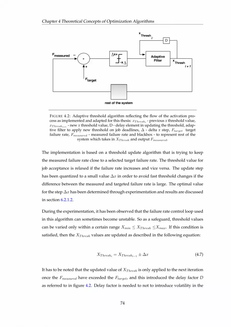
Chapter 4 Theoretical Concepts of Optimization Algorithms
D
+
!!"#$%&'(&)"*+&,-../0& 123&45336&7892"*3:& ;"<3&=&+>&=&
!
123&?":23@":$AB&==&C+@93:3DAE&13B:&
!"#$%&##'$()*"+,#-$&&
F:&$B&GH$:3&A+@@+D&:+&HB3&BE@*+8B&>5+@&:23&45336&"892"*3:&:+&53953B3D:&GH"D:$:$3B&$D&
@":23@":$AB(&&I+H&B2+H8%&JHB:&53<"5%&:23B3&BE@*+8B&"B&BE@*+8BK&HB3%&$D&"&A35:"$D&L"E&*E&
A+D#3D:$+DK&"D%&D+:&"B&2"#$D<&"DE&%33935&$D:5$DB$A&@3"D$D<(&&;5+*"*8E&+D3&53"B+D&:23$5&HB3&$B&B+&
L$%3B953"%&$D&@":23@":$AB&$B&:23$5&%$B:$DA:&B2"93BK&L2$A2&953#3D:B&A+D>HB$+D&L$:2&+H5&HBH"8&
"892"*3:$A&A2"5"A:35B&$D&+5%$D"5E&:3M:(&
&
I+H&%+DN:&2"#3&:+&*3&"*83&:+&B93"6&45336&:+&HD%35B:"D%&@":23@":$ABK&*H:&$:&$B&95+*"*8E&2389>H8&:+&
53A+<D$O3&:23&BE@*+8B&"D%&*3&>"@$8$"5&L$:2&:23$5&D"@3B(&&123&45336&"892"*3:&A+DB$B:B&+>&-P&
A2"5"A:35BK&HBH"88E&L5$::3D&"B&>+88+LBQ&
&
&&
.**#&/+0#$ )12#&/+0#$ 3+4#$ *&13.3/5+-513$
"& #& "892"& &
$& %& *3:"& R*"E:"S&
&& '& <"@@"& &
(& )& %38:"& &
*& +& 39B$8+D& &
,& -& O3:"& RO"E:"S&
.& /& 3:"& R"E:"S&
0& 1& :23:"& R:2"E:"S&
2& 3& $+:"& &
4& 5& 6"99"& &
6& 7& 8"@*%"& &
8& 9& @H& R@TE++S&
:& ;& DH& RDTE++S&
<& =& M$& RMBT3E3S&
>& ?& +@$65+D& &
@& A& 9$& R9T3E3S&
B& C& 52+& R5+3S&
D& E& B$<@"& &
F& G& :"H& R:T+LS&
H& I& H9B$8+D& &
J& KK&L& 92$& R>T3E3S&
M& N& A2$& R6T3E3S&
O& P& 9B$& R9TB$<2S&
Q& R& +@3<"& R+@"E<"S&
&123&UCF1&?":2&==&C+@93:3DAE&13B:&%+3B&D+:&"B6&E+H&GH3B:$+DB&"*+H:&:23&A2"5"A:35B&$D&:23&45336&"892"*3:&%$53A:8E(&&V+L3#35K&$D&B+@3&GH3B:$+DB&+D&:23&:3B:K&:23B3&BE@*+8B&@"E&*3&HB3%&"B&"8<3*5"$A&BE@*+8B(&&12$B&8$B:&$B&95+#$%3%&2353&JHB:&:+&<$#3&E+H&"&53>353DA3&>+5&:23&+5$<$D&+>&BE@*+8B&BHA2&"B&:23B3(&
-x
!!"#$%&'(&)"*+&,-../0& 123&45336&7892"*3:& ;"<3&=&+>&=&
!
123&?":23@":$AB&==&C+@93:3DAE&13B:&
!"#$%&##'$()*"+,#-$&&
F:&$B&GH$:3&A+@@+D&:+&HB3&BE@*+8B&>5+@&:23&45336&"892"*3:&:+&53953B3D:&GH"D:$:$3B&$D&
@":23@":$AB(&&I+H&B2+H8%&JHB:&53<"5%&:23B3&BE@*+8B&"B&BE@*+8BK&HB3%&$D&"&A35:"$D&L"E&*E&
A+D#3D:$+DK&"D%&D+:&"B&2"#$D<&"DE&%33935&$D:5$DB$A&@3"D$D<(&&;5+*"*8E&+D3&53"B+D&:23$5&HB3&$B&B+&
L$%3B953"%&$D&@":23@":$AB&$B&:23$5&%$B:$DA:&B2"93BK&L2$A2&953#3D:B&A+D>HB$+D&L$:2&+H5&HBH"8&
"892"*3:$A&A2"5"A:35B&$D&+5%$D"5E&:3M:(&
&
I+H&%+DN:&2"#3&:+&*3&"*83&:+&B93"6&45336&:+&HD%35B:"D%&@":23@":$ABK&*H:&$:&$B&95+*"*8E&2389>H8&:+&
53A+<D$O3&:23&BE@*+8B&"D%&*3&>"@$8$"5&L$:2&:23$5&D"@3B(&&123&45336&"892"*3:&A+DB$B:B&+>&-P&
A2"5"A:35BK&HBH"88E&L5$::3D&"B&>+88+LBQ&
&
&&
.**#&/+0#$ )12#&/+0#$ 3+4#$ *&13.3/5+-513$
"& #& "892"& &
$& %& *3:"& R*"E:"S&
&& '& <"@@"& &
(& )& %38:"& &
*& +& 39B$8+D& &
,& -& O3:"& RO"E:"S&
.& /& 3:"& R"E:"S&
0& 1& :23:"& R:2"E:"S&
2& 3& $+:"& &
4& 5& 6"99"& &
6& 7& 8"@*%"& &
8& 9& @H& R@TE++S&
:& ;& DH& RDTE++S&
<& =& M$& RMBT3E3S&
>& ?& +@$65+D& &
@& A& 9$& R9T3E3S&
B& C& 52+& R5+3S&
D& E& B$<@"& &
F& G& :"H& R:T+LS&
H& I& H9B$8+D& &
J& KK&L& 92$& R>T3E3S&
M& N& A2$& R6T3E3S&
O& P& 9B$& R9TB$<2S&
Q& R& +@3<"& R+@"E<"S&
&123&UCF1&?":2&==&C+@93:3DAE&13B:&%+3B&D+:&"B6&E+H&GH3B:$+DB&"*+H:&:23&A2"5"A:35B&$D&:23&45336&"892"*3:&%$53A:8E(&&V+L3#35K&$D&B+@3&GH3B:$+DB&+D&:23&:3B:K&:23B3&BE@*+8B&@"E&*3&HB3%&"B&"8<3*5"$A&BE@*+8B(&&12$B&8$B:&$B&95+#$%3%&2353&JHB:&:+&<$#3&E+H&"&53>353DA3&>+5&:23&+5$<$D&+>&BE@*+8B&BHA2&"B&:23B3(&
x+
i + 1
i
Ftarget
Fmeasured
+
--
rest of the system
xThresh
xThresh
AdaptiveFilter
FIGURE 4.2: Adaptive threshold algorithm reflecting the flow of the activation pro-cess as implemented and adapted for this thesis: xThreshi - previous x threshold value,xThreshi+1
- new x threshold value, D - delay element in updating the threshold, adap-tive filter to apply new threshold on job deadlines, ∆ - delta x step, Ftarget targetfailure rate, Fmeasured - measured failure rate and blackbox - to represent rest of the
system which takes in XThresh and output Fmeasured.
The implementation is based on a threshold update algorithm that is trying to keep
the measured failure rate close to a selected target failure rate. The threshold value for
job acceptance is relaxed if the failure rate increases and vice versa. The update step
has been quantized to a small value ∆x in order to avoid fast threshold changes if the
difference between the measured and targeted failure rate is large. The optimal value
for the step ∆x has been determined through experimentation and results are discussed
in section 6.2.1.2.
During the experimentation, it has been observed that the failure rate control loop used
in this algorithm can sometimes become unstable. So as a safeguard, threshold values
can be varied only within a certain range Xmin ≤ XThresh ≤Xmax. If this condition is
satisfied, then the XThresh values are updated as described in the following equation:
XThreshi= XThreshi−1
±∆x (4.7)
It has to be noted that the updated value of XThresh is only applied to the next iteration
once the Fmeasured have exceeded the Ftarget, and this introduced the delay factor D
as referred to in figure 4.2. Delay factor is needed to not to introduce volatility in the
74

Chapter 4 Theoretical Concepts of Optimization Algorithms
system to make sure new threshold value only gets applied the new jobs but not to the
existing running jobs.
Continuing with the earlier example, let’s assume that a job with duration-deadline
ratio xi=0.35 appears in the system when XThresh=0.45. This job is allowed to con-
tinue but eventually it fails. When it fails, since the algorithm has a delay mechanism
built it, this failure triggers the system to recalculate its failure rate which happens to
be at Fmeasured=0.35 where as the hard limit for the target failure rate has been set to
Ftarget=0.25 to force the system to converge to lower measured failure rate. Now since
the system is under performing (by having a larger failure rate then the limit set), this
triggers the algorithm to update XThresh value. The reason to update a new XThresh is
that the present value is making the system under perform rather, and with an updated
value of XThresh the system continues in an iterative process to bring down measured
failure rate.
As a result, the adaptive threshold update mechanism, as described in equation 4.7,
increments the XThresh by 0.1 (∆x) to 0.55. ∆x=0.1 is used here for the sake of exam-
ple. And this cycle continues until and unless measured failure rate is reduced or else
XThresh will get further incremented by 0.1 (new XThresh will become 0.65). If it hap-
pens that there is a certain batch of jobs in the system that are all cpu intensive, long
running and can’t meet their deadlines; then either XThresh will be incremented up to
maximum value of 0.9 and while terminating some jobs which can’t be completed and
introducing new jobs that has the potential to be completed. This way it is always try-
ing to favor a mixed workload types to make sure no particular job suffers execution
deprivation.
A second approach taken to calculate XThresh is by using the Cumulative Distribution
Function (CDF) D(v) to determine the probablity of the success rate for the jobs that
have succeeded in meeting their deadlines as shown in figure 4.3.
The distribution function D(v) is described the probability that a real-valued random
variable V with a given probability distribution will be found at a value less than or
equal to v [129]. It is related to discrete probability P(v) by:
D(v) = P (V ≤ v) =∑V≤v
P (v) (4.8)
75
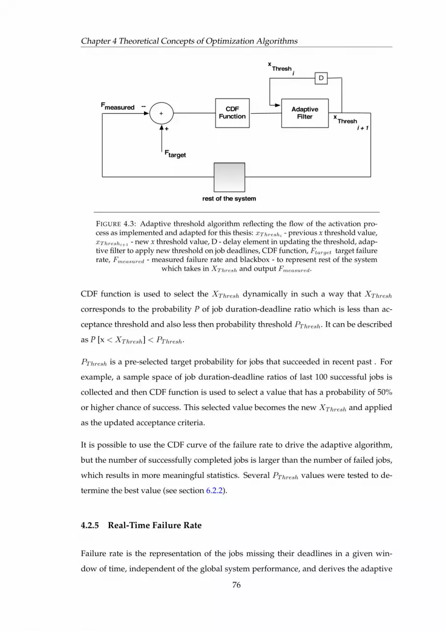
Chapter 4 Theoretical Concepts of Optimization Algorithms
CDFFunction
D
+
i + 1
i
Ftarget
Fmeasured
+
--
rest of the system
xThresh
xThresh
AdaptiveFilter
FIGURE 4.3: Adaptive threshold algorithm reflecting the flow of the activation pro-cess as implemented and adapted for this thesis: xThreshi - previous x threshold value,xThreshi+1
- new x threshold value, D - delay element in updating the threshold, adap-tive filter to apply new threshold on job deadlines, CDF function, Ftarget target failurerate, Fmeasured - measured failure rate and blackbox - to represent rest of the system
which takes in XThresh and output Fmeasured.
CDF function is used to select the XThresh dynamically in such a way that XThresh
corresponds to the probability P of job duration-deadline ratio which is less than ac-
ceptance threshold and also less then probability threshold PThresh. It can be described
as P [x < XThresh] < PThresh.
PThresh is a pre-selected target probability for jobs that succeeded in recent past . For
example, a sample space of job duration-deadline ratios of last 100 successful jobs is
collected and then CDF function is used to select a value that has a probability of 50%
or higher chance of success. This selected value becomes the new XThresh and applied
as the updated acceptance criteria.
It is possible to use the CDF curve of the failure rate to drive the adaptive algorithm,
but the number of successfully completed jobs is larger than the number of failed jobs,
which results in more meaningful statistics. Several PThresh values were tested to de-
termine the best value (see section 6.2.2).
4.2.5 Real-Time Failure Rate
Failure rate is the representation of the jobs missing their deadlines in a given win-
dow of time, independent of the global system performance, and derives the adaptive
76
Chapter 4 Theoretical Concepts of Optimization Algorithms
XThresh values for both delta-based adaptations and for probability based value se-
lection. In delta based adaptation, XThresh is incremented or decremented by a fixed
value to reduce measured failure rate. In probabilistic approach, probability of success
is calculated for recent successful jobs and XThresh is selected based on the probability
of 50% or higher success rate.
Let us denote Fmeasured as the failure rate1 at any given time which we intend to keep as
low as possible than the target failure rate denoted as Ftarget and shouldn’t be greater
then 0.25. This value of 0.25 represents 75% of the base line value, and the objective of
this research is to achieve more than 85% of the physical baseline performance for vir-
tual machine based execution. To calculate Fmeasured, first success rate for last iteration,
denoted as Smeasured, have to be calculated. Fmeasured is then derived by 1 - Smeasured.
To determine Smeasured, there are number approaches that could be used. One is weighted-
alpha method based on leaky-bucket algorithm2 for rate limiter systems or also known
as exponential smoothing technique3. The second approach is using a simple division
of total number of jobs succeeded by total number of jobs in the system at any moment,
and also known as simple moving average4. We have used weighted-alpha method
to calculate the success rate due to its smoothening feature and faster calculation sim-
ilar to leaky-bucket’s traffic shaping function. In this case, the weight-alpha is used to
shape the success rate from jittery state to smooth state.
The exponential smoothing technique uses two factors; weight constant alpha α and
a boolean success constant S. In this particular system, we multiply the success ratio
with the weight factor. Success ratio ( nN ) is derived by dividing the set of n number of
jobs succeeding in meeting their deadline with number of N jobs executed since the last
calculation of Fmeasured. This is shown in equation 4.9.
1Failure rate and Fmeasured terms are used interchangeably in this chapter. They refer and mean thesame parameter.
2The leaky bucket algorithm has several uses, it is best understood in the context of net-work traffic shaping or rate limiting. Typically, the algorithm is used to control the rate atwhich data is injected into a network, smoothing out ”burstiness” in the data rate. See alsohttp://en.wikipedia.org/wiki/Leaky bucket
3Exponential smoothing is a technique that can be applied to time series data, either to producesmoothed data for presentation, or to make forecasts. The time series data themselves are a sequence ofobservations. The observed phenomenon may be an essentially random process, or it may be an orderly,but noisy, process. See also http://en.wikipedia.org/wiki/Exponential smoothing
4In the simple moving average the past observations are weighted equally, ex-ponential smoothing assigns exponentially decreasing weights over time. See alsohttp://en.wikipedia.org/wiki/Simple moving average
77

Chapter 4 Theoretical Concepts of Optimization Algorithms
Smeasured =
(n
N(1− α) + Sα
)(4.9)
The idea behind the formula above is that an updated success rate at iteration t is
heavily weighted towards its previous value (at iteration t-1), and the new success/-
failure value adds a small contribution (weight is alpha). The reason why we introduce
a weighted update of the success rate (where weight is a constant alpha) is to filter out
any burst of failures which would cause the failure rate control loop to oscillate too
much. By adopting a small step alpha, it smoothes out the estimate for the value of the
success rate, which in turn determines the current Fmeasured which is a main parameter
in the system.
This method avoids having to keep track of an ever-increasing number of jobs, and
to avoid the computational overhead of dividing a large number (e.g. 50k jobs suc-
ceeded) by a second large number (e.g. total number of 100k jobs) as compared to sim-
ple division method as shown in equation 4.10. Secondly, by not using moving average
method we avoid giving equal weight to all jobs executed where it is more beneficial to
give higher weight to more recent jobs. This way we utilize a more optimal mechanism
with lower computational overhead and a smaller set of data.
Smeasured =
(JobsSucceededTotalJobs
)(4.10)
Another disadvantage of the moving average based method is that it distorts the results
under certain circumstances e.g. if there is a sudden burst of some additional cpu-
bound jobs in the system, this will result in a spike in the virtualization overhead. At
that time, there could be some long-running jobs executing in the system. Based on the
higher overhead, when the scheduler will re-estimate the deadlines, the longer running
existing jobs will appear to miss their deadlines and if their deadline ratio happens
to be less then XThresh, then these jobs will be terminated. This will result in lower
resource utilization since the terminated jobs have to be resubmitted and re-executed
in the grid. It also prevents the system to quickly respond if the given workload profile
changes completely.
78
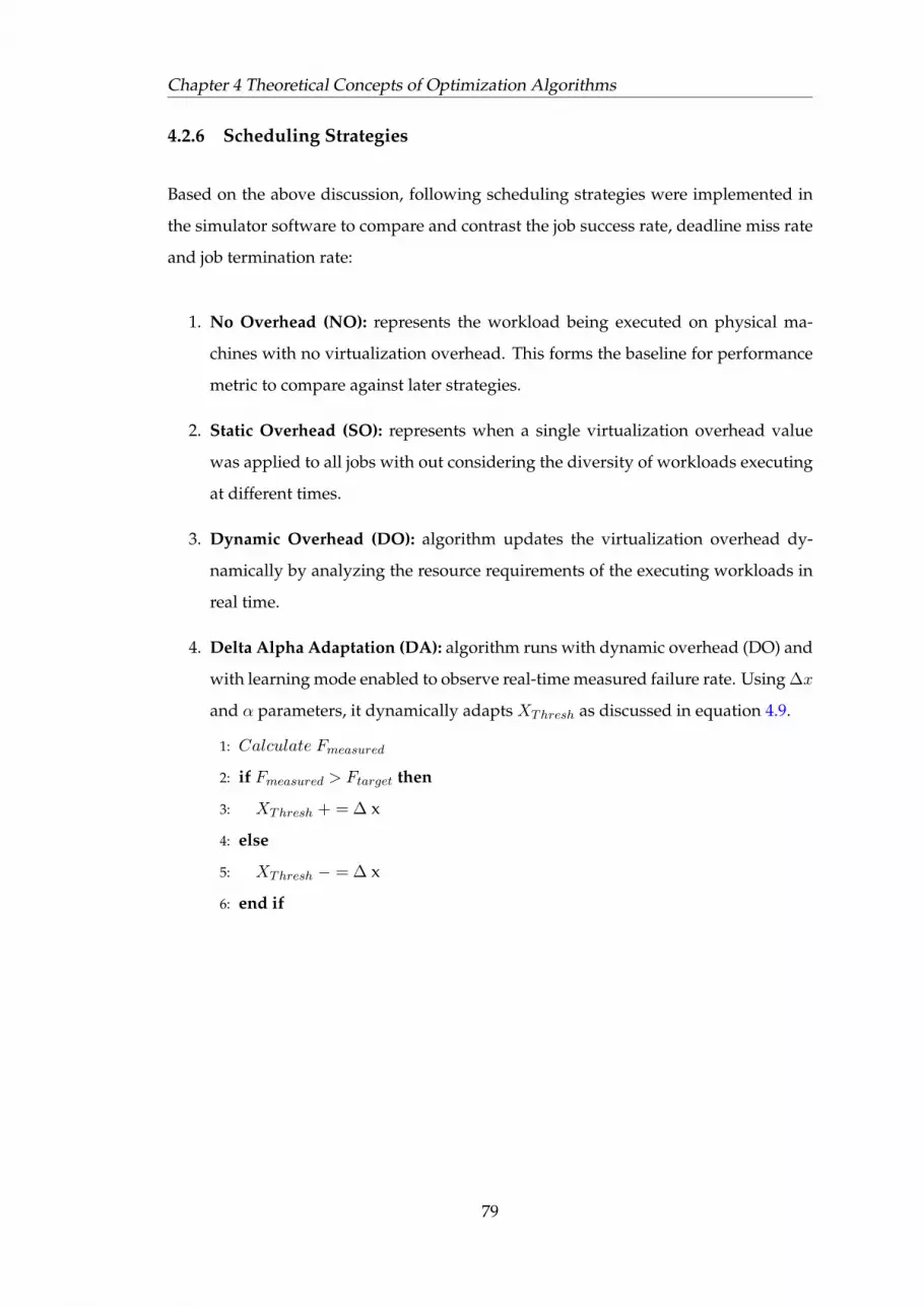
Chapter 4 Theoretical Concepts of Optimization Algorithms
4.2.6 Scheduling Strategies
Based on the above discussion, following scheduling strategies were implemented in
the simulator software to compare and contrast the job success rate, deadline miss rate
and job termination rate:
1. No Overhead (NO): represents the workload being executed on physical ma-
chines with no virtualization overhead. This forms the baseline for performance
metric to compare against later strategies.
2. Static Overhead (SO): represents when a single virtualization overhead value
was applied to all jobs with out considering the diversity of workloads executing
at different times.
3. Dynamic Overhead (DO): algorithm updates the virtualization overhead dy-
namically by analyzing the resource requirements of the executing workloads in
real time.
4. Delta Alpha Adaptation (DA): algorithm runs with dynamic overhead (DO) and
with learning mode enabled to observe real-time measured failure rate. Using ∆x
and α parameters, it dynamically adapts XThresh as discussed in equation 4.9.
1: Calculate Fmeasured
2: if Fmeasured > Ftarget then
3: XThresh + = ∆ x
4: else
5: XThresh − = ∆ x
6: end if
79

Chapter 4 Theoretical Concepts of Optimization Algorithms
5. Probabilistic x Adaptation (PA): algorithm runs with dynamic overhead (DO)
but rather then using small changes to XThresh with ∆x parameter; it uses cumu-
lative distribution functions to analyze the pattern of recent successful jobs and
adapts the XThresh for the executing work loads accordingly.
1: Calculate Fmeasured
2: if Fmeasured > Ftarget then
3: XThresh← Cumulative Distribution Function (PThresh > 0.5)
4: end if
4.3 Summary
This chapter has discussed the rationale behind the development of a simulation sys-
tem to validate optimization techniques. All the theoretical concepts related to assump-
tions made, hypothesis developed and the design and architecture of the simulator are
described. Then the discussion was expanded to the deadline constraints, virtual exe-
cution time that is dependent on virtualization overhead and the performance metrics
which were used in later experiments to validate optimization strategies. This is in line
to answer research question number 3 and is evaluated empirically in chapter 6.
An overview of two key optimization strategies has been presented; delta adaptive and
probability based adaptive algorithms. These technique were further evaluated against
a physical baseline, virtual baseline, static and dynamic adaptation of virtualization
overhead. A detailed discussion was included in this chapter about the workings of
the adaptive algorithms with a block diagram that described that how the adaptive al-
gorithms function and links various parameters such as measured failure rate, XThresh
and its lower and upper limits.
The next chapter provides the results related to the preliminary experimentation which
was done to show the feasibility of virtualization technology for HPC grid jobs and
applications.
80

Chapter 5
ATLAS Job Performance
Experiments
“The question is not what you look at, but what you see.”
Henry David Thoreau
Virtualization technology has a performance overhead, as discussed in chapter 1 and
chapter 3; it is an objective of this thesis to evaluate the feasibility of running HPC
grid jobs in virtual machines. As a result, preliminary experiments were designed and
conducted based on real tasks to evaluate the performance of ATLAS jobs1 in virtual
machines.
This chapter first describes the existing PanDA pilot job submission system and the
modifications made to integrate virtualization into the grid in section 5.1. This was
necessary to have a feasible deployment scenario based on a real grid application. This
implementation approach is applicable to other grid applications as well. In section 5.2,
experimental setup to conduct preliminary studies is defined, and then the empirical
results are presented in section 5.3.
This chapter answers research questions 1 and 2 (see section 1.1). The results presented
in this chapter have also been published in a peer-reviewed conference [4].
1see appendix B
81

Chapter 5 ATLAS Job Performance Experiments
5.1 Existing ATLAS System
This section describes the present ATLAS system for deploying pilot jobs in the grid,
and the modification made to it to integrate virtualization in to the grid infrastructure.
A brief overview of pilot job framework in the context of ATLAS system is also de-
scribed in section 2.2.3. Basically, its a job leasing framework that sends dummy jobs to
the grid to reserve job execution slots at worker nodes.
5.1.1 PanDA Architecture
As shown in figure 5.1, PanDA pilot server sends dummy jobs to the workload man-
agement system (WMS) in the grid middleware which schedules it to a particular grid
site, and the local batch system at the grid site schedules the job on to one of the avail-
able worker nodes and assigns an execution slot. At this point, PanDA pilot establishes
a direct network connection with PanDA pilot server which is external to the grid in-
frastructure. PanDA pilot server manages it’s job queues independent of the grid, and
based on the resource available at the job slot, it selects the job from the server which
fits that criteria and sends it to the remote pilot process.
PanDAPilot
ServerGrid WMS
User Job
Job
Worker Nodes
Job
networkconnectionproduction
automatedsystem
Job
FIGURE 5.1: Grid Pilot jobs overview and the steps it goes through. PanDA serversends empty jobs to the grid WMS to reserve a job slot at a worker node. Once anexecution slot is reserved, then it directly downloads the job to the worker node fromthe server to continue with the job execution, and thus bypasses the grid middlewarethrough peer-to-peer connectivity between the PanDA server and pilot job running in
the worker node.
82

Chapter 5 ATLAS Job Performance Experiments
Once the pilot process finishes downloading the job from the server, it goes through the
following steps to execute the job as shown in figure 5.2:
1. Environment Preparation: After downloading the job, pilot process daemon
prepares the environment and sets the necessary variables on the worker node so
that the job execution can proceed.
2. Data Stage-in: After setting up the environment, the pilot job daemon downloads
the necessary data required to complete the job from the grid storage element.
The network latency to connect to grid storage element and time to download the
data will vary for each job.
3. Job Execution: Once all data is downloaded on the worker node, the pilot job
daemon triggers it’s runJob script to commence job execution. During the lifetime
of the job execution, the runJob script periodically sends the status updates to
the pilot daemon, which then in turn updates the PanDA pilot server with the
progress of the job.
4. Data Stage-out: In this phase, the pilot job daemon updates the final output re-
sults of the job to the grid storage element if the job completed successfully oth-
erwise it sends the error logs to the PanDA server so that it could be debugged
by the user.
5.1.2 Virtualization in PanDA Pilot
5.1.2.1 vGrid Deployment Engine
In this study, vGrid2 tool [1] was used as primary deployment engine which is based
on the Representative State Transfer (REST)3 protocol for inter-node communications.
It deals with tasks such as setting up logical volume partitions, decompressing an op-
erating system image in it, and starting/stopping virtual machines. It provides both
2vGrid tool was developed by the author and is the technical contribution in this thesis. It was modifiedby T. Koeckerbauer to use it to satisfy the use cases of a local project in our team. But this was built andexpanded on the earlier work done by the author of this thesis, and original vGrid was used for the PanDAvirtualization.
3REST-style architectures consist of clients and servers where clients initiate requests toservers; servers process requests and return appropriate responses. For more information, see:http://en.wikipedia.org/wiki/Representational State Transfer
83

Chapter 5 ATLAS Job Performance Experiments
RunJob Script
Pilot Job Daemon
2. Prepare Environment
1. Start Job
3. Execute Job
4. Progress Update5. Cleanup
Panda Server
Internet
FIGURE 5.2: PanDA pilot job submission and stages it goes through to execute a gridjob. Once the pilot job daemon has downloaded the input job data, then runJob scriptsprepares the environment and start executing the job. During execution, periodic up-
date is sent to the pilot job daemon which are further sent to the PanDA server.
web interface for users to deploy virtual machines on demand on pre-configured clus-
ter and REST based interfaces so that it could be integrated into another software, such
as PanDA pilot, to utilize it’s virtualization capabilities.
As shown in the figure 5.3, clients interact with the server through well defined web or
REST interfaces which is responsible to gather all the requirements for virtual machine
such as disk size, operating system for the virtual machine, memory and networking
interface. This information is passed to the vGrid server daemon which then selects the
node through Node Scheduler component which matches these requirements and for-
wards it to Request Forwarder to transmit the information to the selected node through
a peer-to-peer connection. Each node in turn runs a vGrid daemon service where node
Request Handler receive these input parameters and deploys the virtual machines.
Once the virtual machine is deployed and ready to use, server is updated about it sta-
tus and the control of the virtual machine is handed over to the requesting application
which in this case is PanDA pilot daemon.
There are additional components in vGrid server daemon such as Configuration Man-
ager to read configuration files to select which nodes are participating in the virtual
cluster. Similarly, vGrid node daemon have Xen Monitor component that gathers in-
formation for the running virtual machines on each node using LibVirt API [130]. It has
84
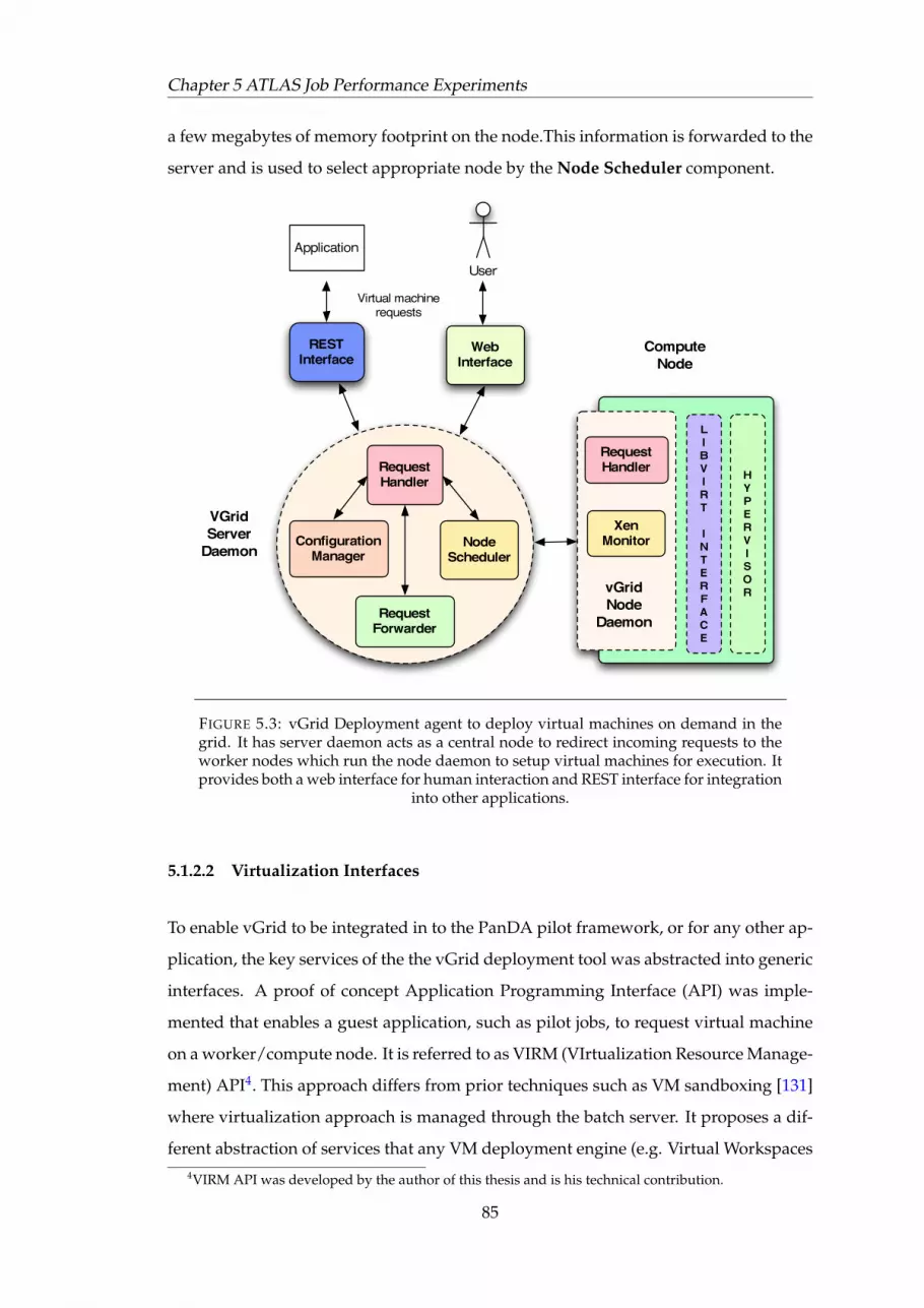
Chapter 5 ATLAS Job Performance Experiments
a few megabytes of memory footprint on the node.This information is forwarded to the
server and is used to select appropriate node by the Node Scheduler component.
User
Web Interface
RESTInterface
ConfigurationManager
RequestHandler
NodeScheduler
RequestForwarder
VGridServer
Daemon
Application
Virtual machinerequests
RequestHandler
XenMonitor
vGridNode
Daemon
ComputeNode
LIBVIRT
INTERFACE
HYPERVISOR
FIGURE 5.3: vGrid Deployment agent to deploy virtual machines on demand in thegrid. It has server daemon acts as a central node to redirect incoming requests to theworker nodes which run the node daemon to setup virtual machines for execution. Itprovides both a web interface for human interaction and REST interface for integration
into other applications.
5.1.2.2 Virtualization Interfaces
To enable vGrid to be integrated in to the PanDA pilot framework, or for any other ap-
plication, the key services of the the vGrid deployment tool was abstracted into generic
interfaces. A proof of concept Application Programming Interface (API) was imple-
mented that enables a guest application, such as pilot jobs, to request virtual machine
on a worker/compute node. It is referred to as VIRM (VIrtualization Resource Manage-
ment) API4. This approach differs from prior techniques such as VM sandboxing [131]
where virtualization approach is managed through the batch server. It proposes a dif-
ferent abstraction of services that any VM deployment engine (e.g. Virtual Workspaces4VIRM API was developed by the author of this thesis and is his technical contribution.
85

Chapter 5 ATLAS Job Performance Experiments
[132], OpenNebula [133]) must provide in the context of Grid application by using lo-
cally available command line linux tools to avoid 3rd party dependencies.
The VIRM API is the abstraction of interaction between external application (i.e. batch
system or PanDA pilot) and the vGrid server daemon. This API have identified key
set of actions that has to be taken by a virtual machine deployment engine to setup
virtual machines. These actions could be implemented in any technology as long as
the external application can execute them via a service end-point, and therefore leads
to standarisation of these actions. These service end-points are following:
• request diskspace: to request a writeable disk partition for the application to
execute its job with a specified operating system.
• mount/unmount diskspace: to have access to the workspace so that application
could customize it and then unmount it a.k.a Contextualization
• start/stop virtual machine: to start and stop virtual machine.
• remove diskspace: to remove the physical disk partition once the job has been
executed.
• send heartbeat: the guest application sends a periodic heartbeat message to the
daemon to keep the virtual machine alive.
From the architectural point of view, VIRM interfaces sit between the deployment
agents and the applications as shown in figure 5.4. The key advantage of having such
an interface is that it enables very many deployment agents, irrespective of their tech-
nology and underlying hypervisor, to interface with grid applications thus pushing
towards the standardization process of communication between grid and virtual ma-
chine deployment tools.
5.1.2.3 Modification to PanDA Pilot
To achieve research objective 1 (see section 1.2 for more details), the PanDA pilot frame-
work was modified to add interface end points for VIRM API, as shown in figure 5.4,
which led to its architectural change [2]. At the deployment phase once the pilot job
86
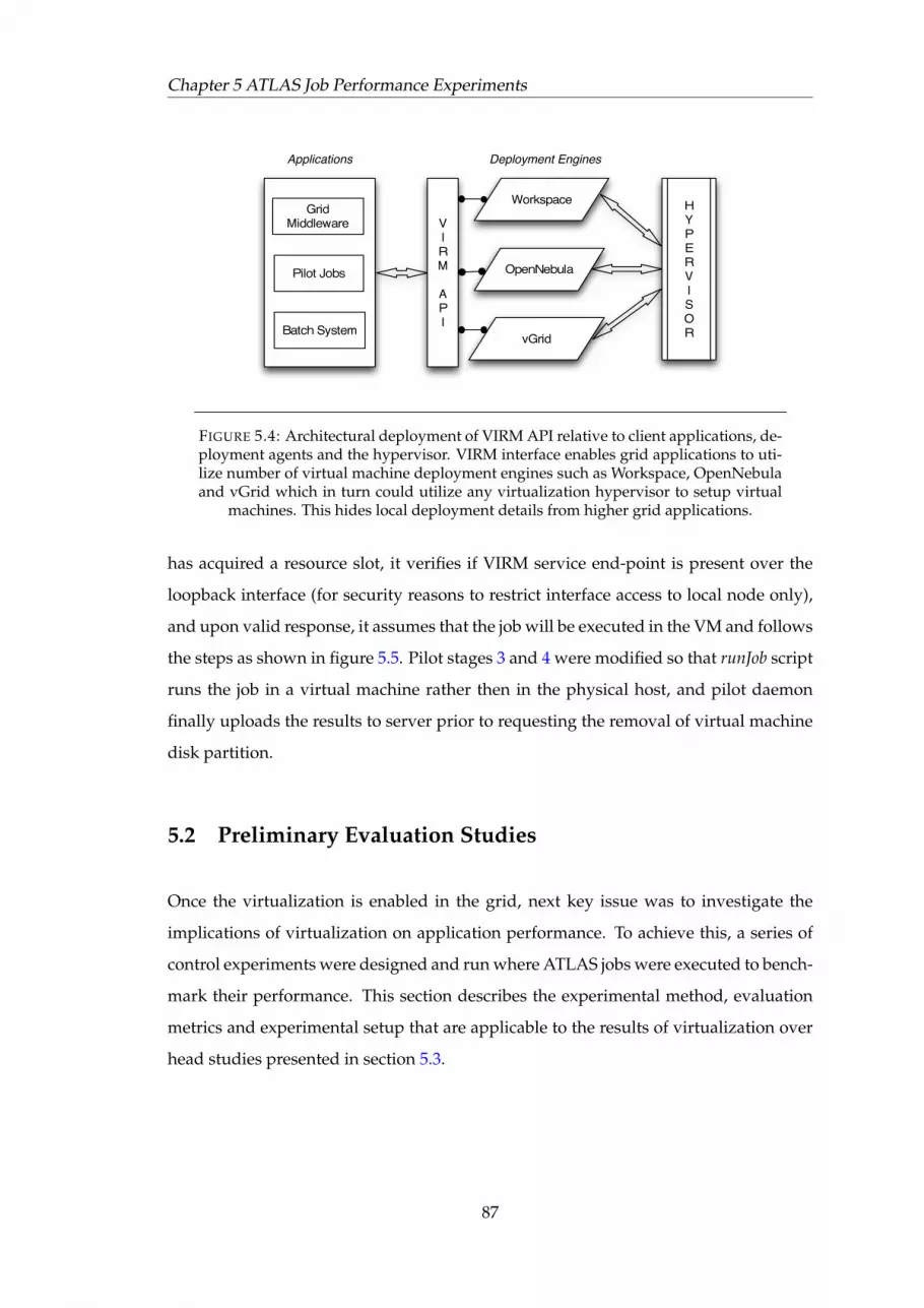
Chapter 5 ATLAS Job Performance Experiments
!"#$
%&"
'()*+,-./
0,/12/345-
67)89
!"#$%&'"()*+(,-(".
:;&<#!"=0#
/##$-01)-%(.
7)89>$8995/?-)/
@-A.B>=C+A/D
&85(A>E(3+
!"#$%&'()*+,%#-*(.&/&0*1*/$(2#-3"$*-$%#*
FIGURE 5.4: Architectural deployment of VIRM API relative to client applications, de-ployment agents and the hypervisor. VIRM interface enables grid applications to uti-lize number of virtual machine deployment engines such as Workspace, OpenNebulaand vGrid which in turn could utilize any virtualization hypervisor to setup virtual
machines. This hides local deployment details from higher grid applications.
has acquired a resource slot, it verifies if VIRM service end-point is present over the
loopback interface (for security reasons to restrict interface access to local node only),
and upon valid response, it assumes that the job will be executed in the VM and follows
the steps as shown in figure 5.5. Pilot stages 3 and 4 were modified so that runJob script
runs the job in a virtual machine rather then in the physical host, and pilot daemon
finally uploads the results to server prior to requesting the removal of virtual machine
disk partition.
5.2 Preliminary Evaluation Studies
Once the virtualization is enabled in the grid, next key issue was to investigate the
implications of virtualization on application performance. To achieve this, a series of
control experiments were designed and run where ATLAS jobs were executed to bench-
mark their performance. This section describes the experimental method, evaluation
metrics and experimental setup that are applicable to the results of virtualization over
head studies presented in section 5.3.
87

Chapter 5 ATLAS Job Performance Experiments
RunJob Script
Pilot Job Daemon
Virtual Machine
2. Prepare Environment
3. Launch Virtual Machine
1. Start Job
4. Execute Job
6. Exit
5. Periodic Progress Update
7. Cleanup
Panda Server
Internet
vGrid
FIGURE 5.5: Once the pilot job has started, it launches the runjob script, which requeststhe virtual machine container from the VIRM agent and starts the job execution. Oncestarted, the virtual machine updates the main pilot job of its status and upon job fail-
ing/termination; the runjob script requests the shutdown of the virtual machine.
5.2.1 Evaluation Metric
First of all, the key issue is to design the measurement metric based on which a quan-
titative observations could be made and qualitative analysis could be derived. Since
the primary factor involved here is the slowing down of the task execution when virtu-
alized, thus the evaluation metric used for CPU and memory related experimentation
concerned with how much time it took to complete the tasks under different system
loads and memory configurations.
Second important metric in this experimentation is networking throughput in virtual
machines. This is critical since each job requires data input that have to be downloaded
from the grid. Thus, for networking related experiments; rate of data throughput was
the key measurement value as performance metric.
88

Chapter 5 ATLAS Job Performance Experiments
5.2.2 Approach and Method
There are three key resource utilization characteristics of ATLAS jobs; CPU intensive-
ness, memory size and network throughput. The experiments were divided based on
these requirements so that the impact of virtualization on them could be evaluated sep-
arately with minimum error and interference from other system conditions. They are
described as following:
1. Network Throughput: ATLAS reconstruction jobs, see table B.1, require large
amount of data to be downloaded over the network. Thus to evaluate network
throughput, a specified data set was downloaded both from physical and vir-
tual source to a virtual machine within the local network to benchmark network
throughput.
2. CPU Evaluations: Xen hypervisor schedules and shares CPU resources among
parallel running virtual machines; as the number of virtual machines increases,
the processing time available for each virtual machine reduces. Since LCG grid
is designed to maximize resource utilization by running as many jobs as possible
in parallel, there by in virtualized environment it would be critical to understand
the impact once the system is run at full capacity. Thus job execution time was
measured by systematically and progressively increasing the number of parallel
virtual machines each running an ATLAS job. The time taken for job execution
when run in a physical machine was set as baseline against which time taken for
job execution in virtual machines was measured.
Once the virtual performance was benchmarked, it was important to optimize
each evaluation metric to improve performance. Therefore, CPU evaluation ex-
periments were ran with two different scheduling techniques namely work con-
serving (WC) and non-work conserving (NWC) (see section 3.4 for more details).
WC is referred to as ”fair-share” and NWC as ”pinned” CPU approach with dif-
ferent weight ratios. The results are presented in section 5.3.2.
3. Memory Evaluations: Memory is another important resource for ATLAS jobs
since some of its detector related algorithms require complex memory operations.
The methodology followed to measure the impact on the size of virtual memory
was that each job running in virtual machine were first executed with maximum
89
Chapter 5 ATLAS Job Performance Experiments
available memory to determine virtual baseline, and then memory size for each
virtual machine was reduced to bare minimum requirement of the job. The ex-
periments were conducted with both high and low system load. The results are
presented in section 5.3.3.
This methodology provides an understanding about how ATLAS jobs will perform in
a virtual machine when run with optimized resources and high utilization rate of the
physical machine resources. All the above experiments and the parameters used are
further elaborated upon in appendix C.
5.2.3 Experiment Design
5.2.3.1 Setup
The test bed used for these experiments consisted of two servers; each with SMP dual-
core Intel CPUs running at 3 GHz, 8 GB Random Access Memory (RAM) and 1 Gbit/s
Network Interface Card (NIC) and running Xen 3.1 [25] hypervisor on Scientific Linux
CERN (SLC) 4.
5.2.3.2 Xen Parameters
There are number of configuration parameters available in Xen5 hypervisor which al-
low fine grained control over its behavior and enables optimized configuration of the
resources available for each virtual machine. The following parameters were adjusted
to measure the above mentioned evaluation metrics:
1. Scheduling Algorithm: There are two scheduling techniques fairshare and pinned
in credit scheduler. Fairshare scheduling is of work conserving mode that allocates
CPU among running VM’s, and additional CPU if its available and no other VM
is competing for it. Xen’s pinned scheduling algorithm, which works in non work
conserving mode, is based on an approach that strictly allocates CPU resources
to a given VM based on CPU capping and weight ratios, and never provides
5The complete reference guide for Xen parameters is available from here:http://bits.xensource.com/Xen/docs/user.pdf
90

Chapter 5 ATLAS Job Performance Experiments
additional resources even if the CPU is running idle. This is discussed in detail in
section 3.4. For CPU metrics, for all the experiments; both scheduling techniques
were used one by one and their performance impact were compared in the context
of ATLAS jobs.
2. CPU Weight: Each VM can be given a weight ratio which is relevant to Xen’s
admin domain calledDom0. Based on weight ratio, Xen credit scheduler allocates
CPU time slot to that particular VM accordingly. Weight ratio 0 means that a VM
gets the same priority asDom0, where as for higher ratios the credit scheduler will
allocate more CPU to a particular VM as a multiple of 256 (a weighting system
used by Xen hypervisor internally to allocate weight) relative to Dom0. In these
experiments, each VM was pinned to a physical CPU and it’s performance was
bench marked with different weight ratios.
3. CPU Capping: If weight ratio is not used to determine the allocation of the CPU,
then credit scheduler can be used to limit it through CPU capping. Each physical
CPU is accessed via a logical abstraction of virtual CPU in the hypervisor. Each
VM then could be pinned to a particular virtual CPU. Then each virtual CPU
could be configured to either use all available physical CPU, only one CPU or half
of the physical CPU for a selected VM. For ATLAS performance studies, virtual
jobs were executed with different CPU capping to arrive at optimal CPU capping
factor where performance loss is minimal and resource utilization is highest.
4. Memory Size: Each megabyte of available system memory could be allocated to
each VM through Xen’s memory ballon driver which is responsible for increasing
or decreasing the size of virtual machine memory.
5.3 Results
This section presents the results from the performance evaluation studies done for AT-
LAS jobs. Primarily reconstruction jobs were used for the experiments since they have
the most demanding resource requirement profile for CPU, memory and networking
resources. See Table B.1 for more details. It is to be noted that Dom0 represents the
virtual machine control domain and doesn’t execute any jobs where as Domi refers to
virtual machine executing an ATLAS job.
91

Chapter 5 ATLAS Job Performance Experiments
These results provide empirical evidence that optimization of Xen scheduling parame-
ters have significant impact on the job performance. In these experiments, as described
in detail in appendix C, 10 different test configurations were used for job execution
measurements and 5 different configurations were evaluated for networking through-
put. Each configuration has different number of allocated CPU (weight and capping
relative to Dom0 - to limit on percentage of CPU available for the VM), memory, and
parallel running Domi.
5.3.1 Network I/O Performance
One of the sources of largest virtualization overhead comes from the network I/O as
Xen hypervisor uses CPU cycles to process network packets as well, and this leads
to additional loss of performance. This is due to Xens virtual network device driver
architecture, which resides in Dom0. See section 3.2.1.2 for more details on this.
The next step was to benchmark the virtual network throughput in Dom0 since in the
bridged configuration all VM’s network packets passes through the Dom0. To bench-
mark this, first network throughput was measured for a data set of 3GB as transfered
from a physical host on the same network with average utilization . This was to ex-
clude the possibility of discrepancy emerging due to reduced traffic during off-peak
hours, and the transfer was restricted to local LAN to prevent external factors of other
network influencing the result. Then, Dom0 memory was progressively halved to 2GB,
1GB and finally 0.5GB for the same data transfer. The tests were ran using Linux scp6 (secure copy) utility on the LAN to avoid external network latencies interfering with
the measurements.
It was observed, as shown in figure 5.6, that Dom0 network throughput dropped sig-
nificantly if constrained to 0.5 GB, but Dom0 I/O throughput improved to ≈50 Mb/s
for the memory range greater than one GB while the average throughput achieved on
physical network was ≈62.5 Mb/s for peak times. The lack of any significant increase
from 1GB to 2GB memory size for Dom0 shows that 1GB is the minimum memory re-
quired by Xen hypervisor to optimally process network packets. After 1GB of memory,
network processing by the hypervisor is not memory-bound any more.
6Linux secure copy command: http://en.wikipedia.org/wiki/Secure copy
92
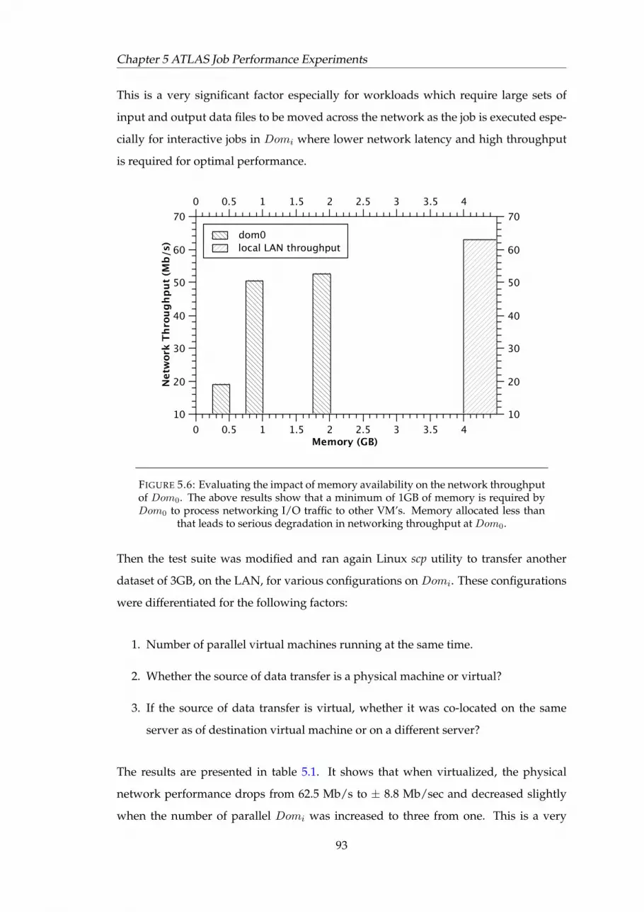
Chapter 5 ATLAS Job Performance Experiments
This is a very significant factor especially for workloads which require large sets of
input and output data files to be moved across the network as the job is executed espe-
cially for interactive jobs in Domi where lower network latency and high throughput
is required for optimal performance.!"#bm$%&'"()m*+(",-.,&
$%&'"()m*+(",-+.,&mk/0M1T
tN
hN
rN
uN
gN
pN
!N
m
tN
hN
rN
uN
gN
pN
!N
/%#"(2mk34TN NLg t tLg h hLg r rLg u
mN NLg t tLg h hLg r rLg u
2"#$N
2%#&'%2()*2+,-#./,0.+
FIGURE 5.6: Evaluating the impact of memory availability on the network throughputof Dom0. The above results show that a minimum of 1GB of memory is required byDom0 to process networking I/O traffic to other VM’s. Memory allocated less than
that leads to serious degradation in networking throughput at Dom0.
Then the test suite was modified and ran again Linux scp utility to transfer another
dataset of 3GB, on the LAN, for various configurations on Domi. These configurations
were differentiated for the following factors:
1. Number of parallel virtual machines running at the same time.
2. Whether the source of data transfer is a physical machine or virtual?
3. If the source of data transfer is virtual, whether it was co-located on the same
server as of destination virtual machine or on a different server?
The results are presented in table 5.1. It shows that when virtualized, the physical
network performance drops from 62.5 Mb/s to ± 8.8 Mb/sec and decreased slightly
when the number of parallel Domi was increased to three from one. This is a very
93

Chapter 5 ATLAS Job Performance Experiments
Parallel Domi Data Source - Data Destination Throughput (Mb/sec)0 Physical-to-Physical 62.81 Physical-to-Virtual 8.83 Physical-to-Virtual 8.33 Virtual-to-Virtual (two different servers) 6.83 Virtual-to-Virtual (on the same server) 6.4
TABLE 5.1: Evaluation of network throughput for physical and parallel runningDomi
by transferring 3GB dataset.
significant reduction in network throughput. The throughput further drops to 6.8 Mb/s
when both source and destination of data are virtualized but deployed on different
servers. And co-locating them on the same server reduces the throughput by further
0.4 Mb/s due to the fact that since their network packets are using the same underlying
CPU for processing, and this introduces additional latency.
These scenarios is important for Grid Storage Element (SE) since if they are virtualized
as well along side of virtualizing job execution, then this further impeds the throughput
for data transfers for various job requests.
The above results provide empirical evidence to show that networking architectures
of the underlying virtualization hypervisor have a significant impact on the available
network throughput for virtual machines. The experiments conducted were to validate
the optimal place to do network transfers when pilot jobs are virtualized. The empiri-
cal results show that all data upload and download in Dom0 rather than Domi for the
HPC workloads provides a significant boost to performance by removing network re-
lated virtualization over head involved for each VM. This study also highlighted that
reduced network throughput in Domi poses a considerable challenge for deploying
grid services on the virtual machines, and have to be further researched to fully under-
stand its impact before grid storage services can be completely virtualized.
5.3.2 Impact of CPU Parameters
In performance studies, phyBase and virtBase represents the physical and virtual base-
lines against which all configuration results are compared. In phyBase, ATLAS jobs were
executed on a physical machine to benchmark highest possible performance baseline.
94

Chapter 5 ATLAS Job Performance Experiments
Configuration Num ofVM
Pi (Num ofCPU cores)
Ti (sec) Relative Overhead (%)
phyBase 0 4 7080 0virtBase 1 4 7130 1
fsLargeVM 2 2 7193 2fsMedVM 3 1 7970 13withCPUCap 3 0.5 12926 83
TABLE 5.2: Performance results for Xen CPU capping parameters when applied toparallel executing virtual machines.
In virtBase, ATLAS jobs were executed in a virtual machine with highest available re-
sources to benchmark maximum performance achievable while incurring some perfor-
mance loss due to virtualization overhead.
A job’s estimated time of completion depends on the number of CPU cores allocated
(denoted as Pi i.e. Pi=1 is one CPU core) to it; so it’s the most important factor in deter-
mining the job performance in these experiments. As seen in table 5.2, fsLargeVM had
a 2% performance overhead with two CPU cores available for it. Where as, when each
VM was pinned to a single core for fsMedVM, then the performance drops by 13% as
compared to the physical baseline of phyBase. Additionally, there were 3 parallel Domi
running in fsMedVM to represent a higher system load where each VM was pinned to
a single core. This could be taken as minimum performance available for ATLAS jobs
when run in virtual machines and pinned to a single CPU core.
On the other hand, to achieve further decline in performance when Pi was capped to
0.5 (restricted to half of one CPU core), the time to complete the job almost increased
by 83% which shows that the relationship between Ti (job execution time) and Pi is
non-linear. Reduction of Pi to below one CPU core could be useful in situations where
a virtual machine could be either paused (saved state that could be restarted later) or
with reduce allocation of CPU to accommodate additional virtual machines.
The above results show that it is important to consider Pi for more complex situa-
tions where diverse set of workloads may run in parallel VM each with different set of
memory and CPU requirements. This may pose a significant challenge for optimally
allocating machine resources to competing Domi, and must be analyzed for a given
application before hand.
95

Chapter 5 ATLAS Job Performance Experiments
One the other hand, if a single CPU is pinned to eachDomi then the overhead (%) stays
below 15%. This is very promising especially in case of fsMedVM where 3 parallelDomi
were run as compared to phyBase physical baseline. Such a performance penalty could
be acceptable given the gains made through virtualization to achieve fine-grained and
portable virtual machine execution environments for large scale distributed systems
which are prone to misconfigurations.
When a different CPU scheduling technique was applied, it was also observed that
fair-share scheduling technique leads to a slightly better performance as compared to
when CPU was pinned for eachDomi as shown in figure 5.7 where larger set of physics
events for workload got processed between the range of 30s-50s. This may be due to
the fact that pinning the CPU for each Domi constrains it even further if other Domi
may not be fully utilizing available CPU cycles. Xen’s credit scheduler gives a slice of
10ms to each Domi while slices for each Domi are re-computed every 30ms [120].!"#U$%&'()*'+U,'%&-./)'
0)12'+U34U56'-78
s
hs
!s
"s
#s
$s
%s
&s
's
U
s
hs
!s
"s
#s
$s
%s
&s
's
!"#U,.1'Ul8rs #s 's h!s h%s !ss
Us #s 's h!s h%s !ss
2()**+,
2-.)/01./+
FIGURE 5.7: Evaluating CPU scheduling parameters: Pinned vs Fairshare strategy forDomi. Fairshare strategy appears to process higher number of events in the VM within 30-60 seconds as compared to pinned approach since it always allocates additional
CPU shares to a VM when no other VM is competing for it.
Similarly, Xen weight ratios, Wi, for CPU allows to influence CPU availability for each
VM by giving them different weights for fairshare scheduling. When 2 parallel Domi
were ran with Wi of 2 and 4 respectively as compared to Dom0, it was observed that
96

Chapter 5 ATLAS Job Performance Experiments!"#U$%&'()
*+,-%.U/0U12%3)4
o
!o
"o
#o
$o
%o
&o
'o
(oU
o
!o
"o
#o
$o
%o
&o
'o
(o
!"#U5&,%UN4uo $o (o !"o !&o "oo
Uo $o (o !"o !&o "oo
2)*+,-.2/0.+12"
2)*+,-.2/0.+12$
FIGURE 5.8: Evaluating CPU scheduling parameters: Weight ratio strategy for Domi.Both weight ratio reflects similar performance as they are both operating in non work
conserving mode, and only allocates CPU shares according to the weight ratios.
varying Wi among Domi only had a limited impact on the job performance where
higher Wi led to a slightly better performance as shown in figure 5.8. This might be
useful for other workloads, but in case of ATLAS workloads both Fairshare and Pinned
scheduling techniques yield comparable performance.
5.3.3 Impact of Memory
The last important factor influencing ATLAS job performance is the available memory
and how fast the application could access the memory from the system. This is impor-
tant as for every additional memory request, it has to first go through underlying vir-
tualization hypervisor and could introduce some delay between memory request and
allocation. The ATLAS workloads, in particular reconstruction jobs, are highly memory
intensive.
In the experiments, memory available in the system, denoted as Mi, was progressively
reduced for each Domi from memory size 8GB to 2GB to observe the resulting perfor-
mance response for the job. Table 5.3 shows that reducing the Domi memory has a
lesser performance impact when compared to number of parallel Domi each running
97
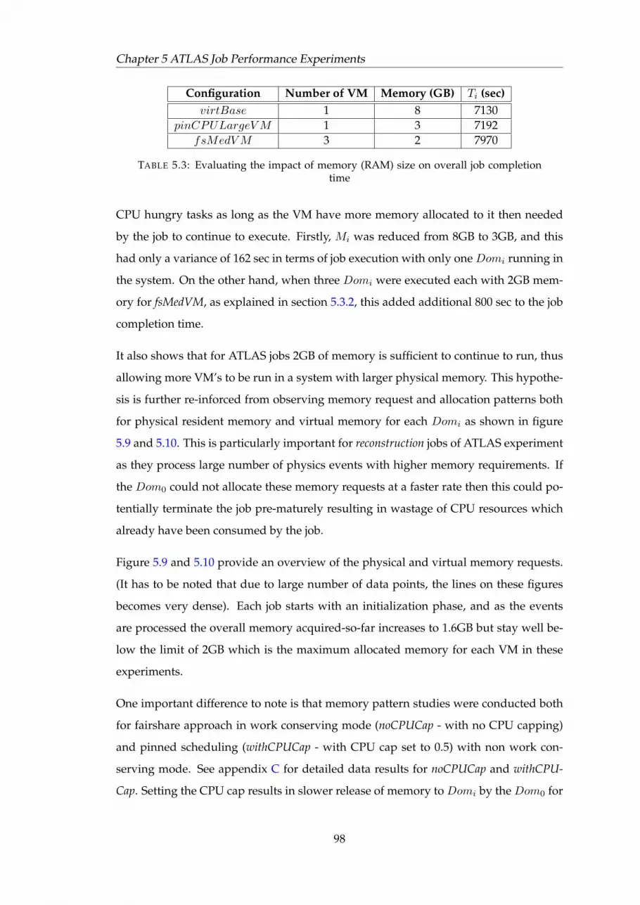
Chapter 5 ATLAS Job Performance Experiments
Configuration Number of VM Memory (GB) Ti (sec)virtBase 1 8 7130
pinCPULargeVM 1 3 7192fsMedVM 3 2 7970
TABLE 5.3: Evaluating the impact of memory (RAM) size on overall job completiontime
CPU hungry tasks as long as the VM have more memory allocated to it then needed
by the job to continue to execute. Firstly, Mi was reduced from 8GB to 3GB, and this
had only a variance of 162 sec in terms of job execution with only one Domi running in
the system. On the other hand, when three Domi were executed each with 2GB mem-
ory for fsMedVM, as explained in section 5.3.2, this added additional 800 sec to the job
completion time.
It also shows that for ATLAS jobs 2GB of memory is sufficient to continue to run, thus
allowing more VM’s to be run in a system with larger physical memory. This hypothe-
sis is further re-inforced from observing memory request and allocation patterns both
for physical resident memory and virtual memory for each Domi as shown in figure
5.9 and 5.10. This is particularly important for reconstruction jobs of ATLAS experiment
as they process large number of physics events with higher memory requirements. If
the Dom0 could not allocate these memory requests at a faster rate then this could po-
tentially terminate the job pre-maturely resulting in wastage of CPU resources which
already have been consumed by the job.
Figure 5.9 and 5.10 provide an overview of the physical and virtual memory requests.
(It has to be noted that due to large number of data points, the lines on these figures
becomes very dense). Each job starts with an initialization phase, and as the events
are processed the overall memory acquired-so-far increases to 1.6GB but stay well be-
low the limit of 2GB which is the maximum allocated memory for each VM in these
experiments.
One important difference to note is that memory pattern studies were conducted both
for fairshare approach in work conserving mode (noCPUCap - with no CPU capping)
and pinned scheduling (withCPUCap - with CPU cap set to 0.5) with non work con-
serving mode. See appendix C for detailed data results for noCPUCap and withCPU-
Cap. Setting the CPU cap results in slower release of memory to Domi by the Dom0 for
98

Chapter 5 ATLAS Job Performance Experiments
Physical Memory Profile
Ph
ysic
al
Resid
en
t M
em
ory
(M
B)
1,275
1,280
1,285
1,290
1,295
1,300
1,305
1,310
1,315
1,275
1,280
1,285
1,290
1,295
1,300
1,305
1,310
1,315
Number of Events-200 0 200 400 600 800 1,0001,2001,4001,600
-200 0 200 400 600 800 1,0001,2001,4001,600
No CPU Cap
With CPU Cap
FIGURE 5.9: Evaluating the impact of parallel running Domi on physical memoryrequests. It shows that CPU capping (non work conserving mode) slows down thememory allocation process due to strict allocation of CPU availability to the VM as
compared to non CPU capping (work conserving).
both physical and virtual memory since it receives lesser CPU cycles to process these re-
quests. As a result, memory requests get queued up and processed only when theDomi
becomes active. Nevertheless both configurations were eventually able to acquire the
memory resources they needed, and the workloads were executed successfully.
Another observation was made that of the incremental increase in the memory alloca-
tion for each job during the course of it’s execution. This is due to a memory-leak bug
in the ATLAS analysis software that leads to memory being not fully released from pre-
vious events while more memory is acquired for next events. This bug was reported
to the ATLAS software developers, and fixing it is beyond the scope and focus of this
study.
These experiments provide further insight into ways that are useful to optimize mem-
ory allocation for ATLAS workloads without large performance penalty.
99

Chapter 5 ATLAS Job Performance Experiments
Virtual Memory Profile
Vir
tual
Mem
ory
(M
B)
1,525
1,530
1,535
1,540
1,545
1,550
1,555
1,560
1,525
1,530
1,535
1,540
1,545
1,550
1,555
1,560
Number of Events-200 0 200 400 600 800 1,000 1,2001,400 1,600
-200 0 200 400 600 800 1,000 1,2001,400 1,600
No CPU Cap
With CPU Cap
FIGURE 5.10: Evaluating the impact of parallel running Domi on virtual memory re-quests. Virtual memory profile is similar to physical memory allocation profile andfollows the same trend where work conserving mode without CPU capping performs
better.
5.4 Summary
This chapter has presented the design and results of preliminary experiments con-
ducted to prove the feasibility of HPC workloads in virtual machines using real-world
tasks and applications, and has addressed two research question number 1 and 2 (see
section 1.1). ATLAS tasks and a job submission application called PanDA pilot were
used in this experiments as a case-study.
In section 5.1, first an overview of the architecture and functionality of PanDA pilot
job framework was given that shows how it deploys ATLAS jobs on the grid. Then
using a virtualization deployment engine, PanDA pilot framework was modified to
deploy the jobs in virtual machines. All the architectural changes required to do this
were described in detail. This has answered research question 1 by providing one of
the ways to integrate virtualization into the grid infrastructure. This model could be
adapted and integrated into other infrastructures as well.
100

Chapter 5 ATLAS Job Performance Experiments
Furthermore, this implementation was influenced by the networking throughput re-
sults which have been presented in section 5.3.1. These results show that it was opti-
mal to use virtualization hypervisor’s administrative domain for networking I/O due
to higher throughput achieve when compared against networking I/O throughput in
virtual machines. This resulted in PanDA implementation downloading and upload-
ing all data in the virtualization administrative domain and using virtual machines
only as execution containers.
In sections 5.3.2 and 5.3.3, results related to execution performance of the tasks were
presented. The results show that ATLAS tasks performance is more sensitive to amount
of CPU cores allocated to them, and if not done optimally, the performance penalty
could go up to 80%. But by optimally using CPU capping and weight parameters in
credit scheduler, the performance overhead could be brought into the range of 5% -
15%.
Similar experimentation related to size and rate of memory allocation showed that de-
spite virtualization overhead, the physics algorithms in ATLAS jobs were able to per-
form well as long as 2GB of memory was available to the virtual machine.
These results have provided answers to research question number 2 by showing that
the workload execution is highly influenced if less then one CPU core per VM is allo-
cated, and if administrative domain runs with less then 1GB of memory that signifi-
cantly reduces network throughput. And the study of the Xen’s credit scheduler pa-
rameters to optimize the performance has shown tangible results that could be applied
to other HPC workloads running in different cloud and grid infrastructures.
This chapter concludes with a demonstration of the feasibility of grid applications and
jobs in virtual machines. The next chapter presents the results related to more advance
optimization techniques evaluated in this thesis to reduce the impact of virtualization
overhead at job scheduling level.
101

Chapter 6
Optimization Experiments for
Deadline Miss Rate
“Who looks outside, dreams.; who looks inside, awakes.”
Carl Gustav Jung
This chapter presents the results of the experiments conducted to empirically evaluate
optimization strategies based on dynamic and adaptive algorithms which were dis-
cussed earlier in chapter 4. Readers of this chapter are suggested to read chapter 4
prior to going through this chapter to make sure that the reader is fully aware of the
theoretical background that led to this experimentation. The empirical data presented
in this chapter provides an understanding to answer research question number 3 re-
lated to optimization of deadline miss rate (see section 1.1).
The flow of the chapter is as follows: section 6.1 describes the experimental design and
an overview of simulation parameters that were necessary for the simulation system
to function. The results section 6.2 is sub-divided into two parts; training phase and
steady phase. In the training phase, different values of simulation parameters were
adjusted and their impact and system response was measured. Then the simulation
were run in steady phase and for longer periods to evaluate the performance of the
adaptive algorithms.
102

Chapter 6 Optimization Experiments for Deadline Miss Rate
6.1 Experimental Design and Rational
The results discussed in this chapter are based on simulated jobs. As explained earlier
in chapter 4, it wasn’t feasible to change or modify the existing grid system at CERN
to test the algorithms since its is being used as a production system. The performance
and preliminary experiments to evaluate virtualization technology for HPC grids jobs
were based on real tasks from CERN’s ATLAS experiment where job execution, cpu
and memory impact and network throughput were studied (see chapter 5). The data
provided by those experiments were sufficient to build the simulator to simulate key
requirements of a worker node in the grid system with a global job queue, and to be
able to apply optimization algorithms to validate them against virtualization overhead
and it’s impact on job throughput and deadlines.
6.1.1 Understanding the Results
The results presented in this chapter are of three different kinds. The first set of results is
related to the overall performance measurements such as system success rate (overall
job throughput), termination rate and deadline miss rate. These results are applica-
ble for both training and steady phases of the simulation. They represent the global
view of the system and are used to differentiate the performance of the optimization
algorithms. An example chart is later shown to familiarize the reader with the results
presented in later sections. The data is separated in three sequential parts; simulation
start-up period, learning period and continuous run period. During simulation start
up period, the simulator begins to gather data and results are very volatile during this
period. Once the system goes to learning period, then it starts collecting data for the
algorithms which would be later used during the continuous run period.
In figure 6.1(a), the performance metric is always plotted on y-axis. This could be suc-
cess rate, termination rate or deadline miss rate depending the nature of the test and
evaluation. On the x-axis, Simulation Time Unit is plotted. Simulation time unit (STU)
metric represents the periodic tick of the scheduler when new schedules are calculated
each time and deadline evaluations are done. It is internal to the simulation engine
and is not directly influenced by the clock speed of the CPU; thus making simulator
executable on different processors of varying speed without affecting the integrity of
103

Chapter 6 Optimization Experiments for Deadline Miss Rate
the results. Higher CPU frequency of the machine where simulations could be run will
only speed up the overall completion time of the simulations. This will not affect sim-
ulated time unit or any other data in that matter. The STU value is set to the average
time of the shortest job life in the queue, which is event generation in ATLAS exper-
iment (see C.1), to make sure all job deadline calculations falls under or within each
scheduling cycle.
In the example chart, the success rate line shows the overall job throughput at any
given moment representing total number of jobs that has successfully completed their
deadlines. The aim is to achieve highest possible value to reflect the positive impact
of algorithmic optimizations. The termination rate line shows the jobs that were termi-
nated either because there weren’t any physical resources available on the system or if
their duration-deadline ratio was less than XThresh acceptance at that time. As a result,
algorithm terminates such jobs which will eventually get resubmitted in the system.
This value should be as low as possible for the optimization algorithms. The last met-
ric is deadline miss rate which shows number of jobs not meeting their deadline at any
given moment. The goal is to keep the value as low as possible.
The second set of results are relevant to two delta adaption and probabilistic optimiza-
tion algorithms only. An example of these results are shown in figure 6.1(b). These
results help understanding how these algorithms operate in determining both real-
time failure rate and XThresh. Real-time failure rate is calculated by using exponential
smoothing technique and only shows the snapshot of the system at a given time. This
failure rate metric helps the system to continuously attempt to converge to lower fail-
ure rates and in the process algorithm’s XThresh values are changed. This is described
in detail in section 4.2.5.
The third set of results are also related to delta adaptation and probabilistic optimiza-
tion algorithms. The graphs, as seen in figure 6.9, shows how long each algorithm takes
to execute and determine new XThresh values. The time measurements for execution is
in real-time (y-axis) and plotted for execution count (x-axis).
104

Chapter 6 Optimization Experiments for Deadline Miss Rate
Performance Metrics
Simulation Time Unit
Continuousrun
period
1.0
Learning period
Simulation startupperiod
success rate
deadline miss rate / termination rate
Legend
Avg. number of jobs Executed
200 1000 10000
100 500 5000
(a) Understanding Algorithmic Performance
Value
Simulation Time Unit
Continuous run period1.0
Learning periodSimulation startupperiod
failure rate
x threshold
Legend
100 500 5000
(b) Understanding Relationship of Real-time Failure Rate and XThreshold
FIGURE 6.1: In first graph, an example of performance curve related to success rate,termination rate and deadline miss rate is shown. This shows the general behavior.The second chart presents the evolution of internal parameters of the algorithms and
their inter-dependent relationship (namely real-time failure rate and XThresh.
105

Chapter 6 Optimization Experiments for Deadline Miss Rate
6.1.2 Experimental Design
While simulating the worker node, machine configuration similar to those of previous
experiments (physical servers) were fed into the simulator. These configurations are
4 CPU cores and 8GB RAM for each simulated server. First simulations were run in
training phase to derive some initial parameters. In this phase, job queue length of
10,000 hours of workloads (1000 jobs) was executed and results were gathered. This
provided sufficient information to tune the initial parameters. Once this was achieved,
then the simulations were run with derived parameters for longer periods and large
job queue length of 100,000 hours of workloads (10,000 jobs). This phase is referred
to as the steady phase for the experiments. The tuning of initial parameters which
were needed for execution and control purposes has direct relevance to the scheduling
strategies. These parameters are explained below:
1. Execution mode: Physical or Virtual - To determine whether to add overhead on
to the job duration. No overhead for physical mode.
2. Overhead mode: Dynamic or Static - To calculate virtualization overhead dy-
namically based on type of executing workload or to keep it static to a single
value. The overhead has been measured from previous experiments, see section
5.3, and it ranges between 5-15% for dynamic scheduling strategies. For static
virtualization, a single value of 15% was used as overhead.
3. CPU Core: Number of CPU’s to be simulated (multiples of 1).
4. Memory Units: Amount of physical memory available in the system (multiples
of 1GB).
5. Alpha α value: The amount of weight added as a smoothing coefficient to calcu-
late success rate which is needed to derive real-time failure rate in the system (see
equation 4.9).
6. Delta Step value: The amount of x threshold to be incremented or decremented
when failure rate is higher or lower than target failure respectively.
7. Target Failure rate: The acceptable failure rate at any given moment in the sys-
tem; beyond which relevant scheduling algorithm 4.2.6 will activate.
106
Chapter 6 Optimization Experiments for Deadline Miss Rate
8. x Threshold: The initial value of x threshold set to during training phase, see
section 6.2.
9. Probability Threshold (PThresh): The initial probability threshold set for the sta-
tistical adaptive algorithm.
6.2 Results
The results for the simulation studies are discussed in detail in this section. As de-
scribed earlier, scheduling simulator have to be trained for auxiliary parameters before
core algorithms, section 4.2.6, to be evaluated. Thus, first the results of the training
phase of these parameters are presented followed by results from the steady phase of
the experimentation.
6.2.1 Training Phase
As mentioned earlier, there are many different input parameters in the simulation such
as memory and CPU, frequency of the scheduler, deadline buffer (set to 5% of the job
duration to represent tight deadlines), alpha α and delta ∆x values for the delta adap-
tive algorithm.The simulator was first run in the training mode to measure optimal
values for the above-mentioned parameters before running the actual simulation. In
this section, results of this training phase are presented.
6.2.1.1 Resource Optimization
ATLAS experiments have a policy to allocate one CPU core for each job [134]. This
is to prevent job starvation as its workloads are of mixed type with different require-
ments for machine resources and has different execution times. Broadly they could be
categorized into short (2 - 6 hrs), medium (6 - 12 hrs) and long (12 - 24 hrs) durations.
In pervious ATLAS experiments, see chapter 5, the impact of amount of CPU and mem-
ory allocation on the job execution was studied with real jobs. Therefore, it was deemed
appropriate to study their impact on overall job throughput and termination rate of the
simulator especially to validate the perviously determined resource allocation for each
107

Chapter 6 Optimization Experiments for Deadline Miss Rate
job. ATLAS job performance studies have shown that 2GB of memory for each CPU
core, when executed in a VM, results in near-optimal performance that tilts the balance
in favor of virtual machine based execution. Secondly, it is important to keep overall
termination rate of jobs low in the system to make sure overall system utilization rate
also stays high.
For the resource allocation related experiments presented in this section, four resource
ratio are defined; res1, res2, res3, res4. These resource ratio represents amount of mem-
ory (GByte) allocated for one CPU core. These ratios were set to 1GByte per CPU core,
1.5GByte per CPU core, 2 and 3 GByte per CPU core respectively. Resource ratio can
also be expressed as resi =M
Cwhere M denotes memory (GByte) and C donates num-
ber of CPU core on the compute node.
Training simulations were ran for these four different resource ratio configurations.
Figure 6.2 shows the results for these experiments. In these graphs, success rate and
job termination rate is plotted on y-axis as a ratio, therefore the maximum possible
value is 1.0 which represent the highest possible success rate or termination rate. The
data points were collected periodically for every scheduler cycle which is measured in
simulation time and plotted on x-axis. For these experiments, termination rate only
included jobs that were cancelled due to lack of availability of machine resources.
In the first graph, res3 and res4 achieves highest over all success rate. res1 has lowest
success rate which shows that most of the time limited machine resources were busy
and any new jobs keep on getting terminated prematurely. Similarly, termination rate
is lowest for res3 and res4 (not clearly seen on the graph as it hovers around 0.0 on y-
axis). Additional results related to overall resource utilization rate are further discussed
in appendix F.
For all other experiments, res3 (2 GByte of memory per CPU core allocated to each VM)
was used as a golden middle for resource ratio with highest success rate and lowest ter-
mination rate. This also matches the configuration of physical servers used in ATLAS
performance experiments which is necessary to make sure simulated conditions are
closer to the real system as discussed in chapter 5.
108

Chapter 6 Optimization Experiments for Deadline Miss Rate
0 100 200 300 400 500Simulation Time Unit
0.0
0.2
0.4
0.6
0.8
1.0
Succ
ess
rate
Success Rate Performance
res_2 success
res_3 success
res_1 success
res_4 success
0 100 200 300 400 500Simulation Time Unit
0.000.050.100.150.200.250.300.350.400.45
Term
inati
on r
ate
Termination Rate Performance
res_2 termination
res_4 termination
res_3 termination
res_1 termination
FIGURE 6.2: Job Success and Termination rates for different resource ratios. The firstgraph shows success rate results where res3 has one of the highest success rate andres1 has the lowest. The second graph plots termination rate for all four configurations
where both res3 and res4 has the lowest job termination rate.
6.2.1.2 Alpha and Delta x Optimization
The next step was to train the algorithm to select initial alpha α and ∆x values1 which
could be then used for the steady phase. These parameters are linked to how fast delta
adaptation algorithm should react whenever real-time failure rate exceeds the set tar-
get. This is explained in more detail in section 4.2.4.
Alpha α represents the weight that is added to the success rate when real-time failure
rate is calculated (see also section 4.2.5). A very high value of alpha α will result in
triggering the algorithm to take action when it might not be necessary, and too low
alpha α can result in very slow response from the algorithm. Similarly, a very high
value of ∆x will result in the acceptance criteria to be changed too much that defeats
the purpose of closely following the behavior of jobs failure rate in the system, and a
1Marked as alpha 1, alpha 2 and alpha 3 for alpha αi and marked as delta 1, delta 2 and delta 3 for∆x values on the graph.
109

Chapter 6 Optimization Experiments for Deadline Miss Rate
very low value of ∆x will cause a very slow change in acceptance threshold leading
to lower job throughput since more jobs will get prematurely terminated. Therefore, a
suitable ratio has to be determined for these two parameters. This is further described
in equation 4.7 and 4.9.
Due to the interlink between these parameters, various trials were made and it was ob-
served during training phase that as long as their inter-ratio was some where between
a factor of 5 to 10 then it keeps the two control loops separate (alpha α to calculate
Fmeasured and ∆x to update XThresh). It was noted that their effective values resided
some where around the range of 0.05 - 0.1.
Therefore, first training phase experiments were run with a constant ∆x value of 0.1
while three different values of alpha α(0.01, 0.05, 0.1) were tested. These three config-
urations for alpha α are labelled as α1, α2, α3. Then the experiments were run in the
reverse order with one value of alpha α=0.05 for three different ∆x values (0.05, 0.1 and
0.2) labelled as configurations ∆x1, ∆x2, ∆x3.
The final and summarized results, as seen in figure 6.3, show the evolution of overall
deadline miss rate for both sets of experiments. Both charts in the figure shows that af-
ter initial simulation start up noise; deadline miss rate begins to converge in the range
of 0.14 - 0.18 for all values of alpha α and ∆x. This is expected behavior since the algo-
rithm is supposed to converge to a value beyond which it can’t optimize. That limit in
optimization is due to the fact that some jobs will be terminated to allow those jobs that
could succeed despite being missing their deadline due to underlying virtualization
overhead. That’s why the aim is to select near-optimal values so that this convergence
takes place as fast and as smoothly as possible.
The system is not influenced by the job arrival rate as new jobs are only introduced into
the worker node once a slot is available, otherwise the job is kept in waiting stage. This
approach is similar to the one deployed on production grids.
The mean values of α and ∆x for overall success rate and deadline miss rate are shown
in table 6.1. These results shows that α2=0.05 and ∆2=0.1 achieved the highest success
rate of 0.93 with lowest deadline miss rate of 0.14. This confirms that these are the best
values for success rate, deadline miss rate and overall convergence rate; therefore these
values were selected as initial values for the steady phase of the experimentation.
110

Chapter 6 Optimization Experiments for Deadline Miss Rate
0 100 200 300 400 500 600Simulation Time Unit
0.0
0.1
0.2
0.3
0.4
0.5
Deadlin
e m
iss
rate
Alpha Training Results
alpha_2
alpha_3
alpha_1
0 100 200 300 400 500 600Simulation Time Unit
0.0
0.1
0.2
0.3
0.4
0.5
Deadlin
e m
iss
rate
Delta Training Results
delta_3
delta_1
delta_2
FIGURE 6.3: Deadline miss rate results for three configurations of Alpha α and Delta∆x values. Both graphs show that deadline miss rate converges to the point beyondwhich the algorithm can’t optimize. This convergence value is in the range of 0.14 -
0.18.
Configuration 1 Configuration 2 Success Rate Deadline Miss Rateα1=0.01 ∆x2=0.1 0.92 0.17α2=0.05 ∆x2=0.1 0.93 0.14α3=0.1 ∆x2=0.1 0.90 0.18
∆x1=0.05 α2=0.05 0.92 0.16∆x2=0.1 α2=0.05 0.93 0.14∆x3=0.2 α2=0.05 0.93 0.15
TABLE 6.1: Performance results for α and ∆x training configurations. The resultsshows that both α2 and ∆x2 achieved highest success rate and lowest deadline miss
rate.
This is further confirmed that for α2=0.05, ∆x3=0.2 begins to show the affects of fast
convergence and for ∆x2=0.1, α3=0.1 results in a stable data line. Therefore, α2=0.05
and ∆x2=0.1 were selected as they begin to affect each other’s performance positively,
and thus are adequate for steady phase.
111

Chapter 6 Optimization Experiments for Deadline Miss Rate
6.2.2 Threshold Determination
Similar tests were run to train the algorithms for initial values for XThresh since this is
one of the most important parameter in the system. It is used by both delta adaptation
and probability algorithms although each of them determines the value in a different
way. XThresh acts as an acceptance criteria for these two algorithms.
If the acceptance is too high or too low then algorithms efficiency is reduced since
there is no room for it to optimize. A very lenient acceptance threshold will result in
increased job submission/acceptance by the scheduler which will increase job deadline
miss rate as some jobs cannot be optimized. A very strict acceptance rate will result
in more jobs being prematurely terminated, and hence decreasing the overall system
success rate.
The threshold level is learnt and adapted by the algorithms automatically in real-time
as deadline miss rate goes up or down. Therefore, a maximum and minimum value are
also set for XThresh to make sure that algorithms don’t go out of valid XThresh range
incase of a sudden rise or fall in deadline miss rate. The maximum limit for XThresh is
0.9 and minimum value is 0.1, and both algorithms try to select best performing values
with in this range during their execution.
The results presented in this section are to determine initial value of XThresh for each
of the algorithms. An appropriate initial value will result in faster convergence to the
steady phase and near optimal performance. The results for these experiments are
discussed in the following sub-sections.
6.2.2.1 Delta Adaptation Algorithm
Delta adaptation (DA) algorithm ((see section 4.2.6, algorithm 4) selects the value by
making smaller increments or decrements to XThresh. The increment or decrement
step is ∆x and set to 0.1 as derived from previous experiments. Five sets of initial
XThresh values were identified; 0.3, 0.4, 0.5, 0.6 and 0.7. The objective here was not
to test all possible values since the algorithm will learn the appropriate value during
runtime, that is why 0.2 and 0.8 were excluded as they are too close to the minimum
and maximum limits. These values were then tested during the training phase.
112
Chapter 6 Optimization Experiments for Deadline Miss Rate
The results from the experiments are presented in 6.4 showing only overall success rate
and termination rate. Deadline miss rate data is not relevant in the selection of initial
XThresh as the aim here is to select a value that enables the system to learn and converge
quicker at the start up of the simulations between 0 - 200 Simulation Time Unit (STU).
The first chart 6.4(a) shows the success rate profile for different XThresh configurations.
XThresh values of 0.3 and 0.4 were slower to increase their initial success rate and went
up to 0.85. This shows that perhaps the initial values were too low and algorithm
responded slowly to optimize success rate. On the other hand, XThresh values of 0.5,
0.6 and 0.7 shows similar success rate profile. They manage to converge to a success
rate value of higher than 0.8 by 50 simulation time units.
This provides one half of the information that an initial XThresh value lies some where
between 0.5 - 0.7. To further tune the XThresh value between 0.5 - 0.7, let’s look at
termination rate data in chart 6.4(b). It shows that 0.7 value for XThresh converges
slower than other values between 0 - 200 simulation time units. This implies that this
value is higher than the near-optimal value of XThresh, and therefore algorithm tried
to reduce it using delta function as seen from the descending stair-like behavior. This
leaves XThresh values of 0.5 and 0.6 where former shows a smooth convergence and
latter has lowest termination rate during initial phase.
Based on these results, XThresh value of 0.6 was selected as initial value for delta adap-
tion algorithm as its flexible (slightly higher than 0.5) and performs well for overall
success rate and termination rate.
113

Chapter 6 Optimization Experiments for Deadline Miss Rate
0 100 200 300 400 500 600Simulation Time Unit
0.0
0.2
0.4
0.6
0.8
1.0
Succ
ess
rate
xthr 0.4
xthr 0.5
xthr 0.3
xthr 0.6
xthr 0.7
(a) Success rate evolution for XThresh values ranging between 0.3 - 0.7. The initial values of 0.5 - 0.7 appearsto achieve a higher success rate much faster than the other values between 50 - 200 simulation time unit.
0 100 200 300 400 500 600Simulation Time Unit
0.00
0.02
0.04
0.06
0.08
0.10
0.12
Term
inat
ion
rate
xthr 0.4
xthr 0.5
xthr 0.3
xthr 0.6
xthr 0.7
(b) Termination rate evolution for XThresh values ranging between 0.3 - 0.7. All values shows a value lowtermination rate and converges to a value less than 0.02 by the end of the simulations.
FIGURE 6.4: Job success rate and termination rate for five configurations of XThresh todetermine the starting value during the steady phase.
114

Chapter 6 Optimization Experiments for Deadline Miss Rate
ProbabilityThreshold
Overall SuccessRate
Deadline MissRate
0.5 0.87 0.180.6 0.85 0.190.7 0.85 0.190.8 0.84 0.200.9 0.83 0.21
TABLE 6.2: Performance results for Probabilistic Adaptation (5) optimization algo-rithm to determine probability threshold.
6.2.2.2 Probabilistic Adaption Algorithm
Probabilistic Adaptation algorithm (algorithm 5 in section 4.2.6) uses cumulative dis-
tribution function to determine XThresh. To achieve this it requires to build a sample
space first, and then execute the functions on the collected data. To achieve this one has
to filter the date set based on a probability value.
This probability value is referred to as Probability threshold (PThresh). It represents the
probability of success of a job for a given XThresh at any given time. e.g. 0.5 PThresh
represents that CDF function should select a XThresh value which has 50% or higher
probability of success based on the collected sample space; this will vary over time as
the rate of job success and failure changes during the course of simulation.
The training phase for PA algorithm was run with initial XThresh value of 0.6 as se-
lected in the previous experiments and five different sets of PThresh were tested against
it. The set of values of PThresh were: 0.5, 0.6, 0.7, 0.8 and 0.9. Values less then 50%
probability (PThresh<0.5) were excluded from testing. The rational behind this is that
the jobs with a lower probability of success than 50% will be terminated, resulting in
lower utilization.
Table 6.2 shows the performance comparison for these values. Experimental results
suggest that by increasing the success probability threshold from 0.5 to 0.9; reduces
overall system success rate and increases deadline miss rate. This is primarily because
it reduces the range of value of job duration-deadline ratios that succeeded, and as a
result PA algorithm selects higher XThresh which causes more jobs to be terminated -
hence higher deadline miss rate. Based on these results, 0.5 success probability thresh-
old appears to a good starting point for this algorithm.
115

Chapter 6 Optimization Experiments for Deadline Miss Rate
For these experiments, initial value XThresh was set to 0.6. During experimentation
with PThresh = 0.5, it was observed that the algorithm selected a value of 0.25 for
XThresh once it was activated (shown in figure 6.5). This value was held constant as
compared to the DA algorithm (see section 6.2.2) which has to adapt XThresh step by
step as failure rate fluctuates. In this case, the failure rate didn’t go beyond the target
failure rate and therefore the algorithm kept the XThresh constant. Based on the above
experiments, the initial values of PThresh=0.5 and XThresh=0.25 were selected for PA
algorithm in the steady phase of the simulations.
FIGURE 6.5: XThresh and real-time failure rate evolution for PA algorithm. It showsthat PA algorithm process of selecting XThresh is much more stable and less volatile.
The initial value of XThresh for PA algorithm seems to be around 0.25.
116

Chapter 6 Optimization Experiments for Deadline Miss Rate
6.2.3 Steady Phase
6.2.3.1 System Performance
Once the key initial values for the simulation parameters were determined during the
training phase, then the experiments were run for a longer period of time to evaluate
the performance of the algorithms. To achieve this, simulated job queue was extended
to have more than 10k job (100,000 execution hours) for each of the five sets of schedul-
ing strategies, as described in section 4.2.6, to simulate ATLAS workloads running on
virtual machines.
Standard strategies
The five strategies are divided into two groups to provide a comparison between the
results. The first group consisted of the following:
1. No Overhead (NO) for physical baseline.
2. Static Overhead (SO) based execution with fixed value of overhead of 15%.
3. Dynamic Overhead (DO) based execution where overhead is set to either 5%, 10%
or 15% depending on the profile of the jobs. If only memory intensive jobs are
running, then the overhead drops to the lowest. If mixed workload are running
the overhead is set to 10%. If CPU intensive overhead’s are running, then 15% of
overhead is set.
The results for the simulation related to the first group are shown in figure 6.6 with
separate results for overall success rate and deadline miss rate. It shows that physical
baseline (NO) has highest success rate as expected since theoretically no job will miss
their deadline in absence of virtualization overhead for these experiments. For the
second strategy when overhead is applied statically (SO) irrespective of the nature of
the jobs running, then success rate drops to around 0.45 and deadline miss rate reaches
to highest level of value 0.55. This helps in defining an optimization space for overall
system success rate and deadline miss rate which lies between the boundaries of NO
and SO upper and lower bounds respectively.
117

Chapter 6 Optimization Experiments for Deadline Miss Rate
Now theoretically speaking, if the virtualization overhead is to be applied dynamically
(DO) depending on the nature of jobs being executed (CPU intensive or memory in-
tensive); then the results should be between NO and SO strategies. The results for DO
strategy shows that success rate improves by 30% and deadline miss rate is reduced to
25% as compared to 55% in SO. This result is not surprising as the jobs in the global
queue are of mixed types and randomized; therefore virtualization overhead in DO
strategy hovers between 5% and 15%.
The interesting aspect in these results is that deadline limit is set to 5% for all jobs
meaning that their deadlines are only +5% in addition to their required duration. Now
with dynamic overhead range up to 15%, the results shows that 75% of the physical
performance is achievable. This was also shown by the experiments conducted for real
ATLAS tasks running in Xen virtual machines (see chapter 5 for more details).
0 1000 2000 3000 4000 5000Simulation Time Unit
0.0
0.2
0.4
0.6
0.8
1.0
Succ
ess
rate
NO/SO/DO Success Performance
SO success
DO success
NO success
0 1000 2000 3000 4000 5000Simulation Time Unit
0.0
0.1
0.2
0.3
0.4
0.5
0.6
0.7
Deadlin
e m
iss
rate
NO/SO/DO Deadline Performance
SO deadline
DO deadline
NO deadline
FIGURE 6.6: Job Success and Deadline miss rates for NO, SO and DO algorithms.Physical baseline (NO) has the highest success rate. By applying virtualization over-head statically (SO) reduces success rate and increases deadline miss rate. For dy-namically adjusted overhead (DO), the system performance is improved by 30% forsuccess rate and deadline miss rate is brought down to 25% when compared against
static overhead.
118

Chapter 6 Optimization Experiments for Deadline Miss Rate
Algorithm Overall SuccessRate
Deadline MissRate
Delta Adaptation 0.83 0.20ProbabilisticAdaptation
0.87 0.17
TABLE 6.3: Performance results for Delta Adaptation (4) and Probabilistic Adaptation(5) optimization algorithms
It has to be noted that so far no optimization algorithm has been applied. This is to
make sure that simulator is able to reproduce results which are aligned with previous
studies to reduce margin of error in simulations. Once the performance results of 75%
are achieved with the simpler approach of DO, it opens up a window of optimization
between 75% and 99%.
Optimization strategies
The second set of strategies consist of two optimization techniques described in chapter
4. They both use dynamic adaptation of virtualization overhead (DO) and are grouped
together to compare them against each other:
1. Optimization algorithm based on Delta ∆x adaptation of XThresh (DA).
2. Optimization algorithm based on probabilistic threshold to select XThresh (PA).
An overview of the final averaged results for success rate and deadline miss rate is
shown for these techniques in table 6.3. Both algorithms have managed to increase
success rate from 0.75 of DO strategy to 0.83 for DA and 0.87 for PA algorithms. The
average of DA and PA success rate is 0.84 which is 7.7% higher then DO. For deadline
miss rate, PA algorithm has performed better than DA. This is primarily because it
uses a more accurate mechanism to select appropriate XThresh value using cumulative
distribution function which results in lower termination rate.
On the other hand, DA algorithm employs different mechanism which takes longer
time to select an appropriate XThresh value and during this period results in termina-
tion of some jobs. The average of DA and PA deadline miss rate is 0.185 which is 20%
less then simpler dynamic adaptation strategy.
119

Chapter 6 Optimization Experiments for Deadline Miss Rate
0 1000 2000 3000 4000 5000 6000Simulation Time Unit
0.0
0.2
0.4
0.6
0.8
1.0
Succ
ess
rate
DA/PA Success Performance
PA success
DA success
0 1000 2000 3000 4000 5000 6000Simulation Time Unit
0.00
0.05
0.10
0.15
0.20
Deadlin
e m
iss
rate
DA/PA Deadine Performance
PA deadline
DA deadline
FIGURE 6.7: Job Success and Deadline miss rates for DA and PA algorithms. Bothalgorithms follows similar trajectories for success rate. For deadline miss rate, PAalgorithm adapts slowly and smoothly where as DA algorithm is more reactive and
volatile.
Figure 6.7 shows the evolution of success rate and deadline miss rate for DA and PA
strategies. It has to be noted that deadline miss rate shown in this figure is cumulative
figure of aggregated deadline missed during the whole simulation, and therefore has
an upward trend. As shown in the second chart, PA data line maintains a more smooth
transition while deadline miss rate rises between 1000 and 5000 simulation time units.
On the other hand, DA algorithm is faster to respond due to small incremental changes
made to XThresh to reduce real-time failure rate but that makes the algorithm slightly
more reactive for deadline miss rate profile between 0 - 500 simulation time units.
After seeing how deadline miss rate evolves for either of the strategies, it’s quite re-
vealing that how both algorithms differ internally while selecting XThresh as shown in
figure 6.8. It shows the evolution of real-time failure which is calculated dynamically
using exponential smoothing technique and is the triggering point for both algorithms.
This results in adaptation of XThresh to reduce the measured failure rate.
120

Chapter 6 Optimization Experiments for Deadline Miss Rate
(a) DA x threshold and failure rate evolution
(b) PA x threshold and failure rate evolution
FIGURE 6.8: XThresh and failure rate evolution results for Delta Adaptation (4) andProbabilistic Adaptation (5) optimization algorithms. Delta Adaptation algorithm re-sulted in a very volatile XThresh value as compared to Probabilistic Adaptation algo-
rithm.
121

Chapter 6 Optimization Experiments for Deadline Miss Rate
Figure 6.8(a) shows that DA algorithm is very reactive and it’s XThresh goes up and
down between maximum and minimum ranges many times whenever it is unable to
reduce real-time failure rate. Contrarily, PA algorithm selects the threshold using a
probabilistic approach from a sample space and makes it more accurate and stable. As
seen from figure 6.8(b), it slowly changesXThresh from 0.25 to 0.15 in response to failure
rate fluctuations. Eventually both algorithms deliver similar performance results. In
both figures, real-time failure rate is very volatile as it is set to change quickly so that
adaptive algorithm gets activated.
6.2.3.2 Algorithmic Execution Performance
The performance results from the previous section have shown that PA is slightly better
than DA algorithm in achieving higher success rate, lower deadline miss rate and stable
evolution of XThresh. There is another aspect to these algorithms that require attention,
and that is their execution time; how fast they execute. Along side performance results,
their execution time was measured in real time to evaluate what sort of algorithmic
overhead footprint they might have.
By looking at the execution of the two algorithms over the course of the experimenta-
tion reveals that DA algorithm takes far less time than PA algorithm as shown in figure
6.9. This is due to the fact that DA algorithm uses a delta step to update XThresh and
this process is very fast as it requires few CPU cycles. On the other hand, PA algorithm
first updates its sample space; then apply cumulative distribution function to select the
next value for XThresh which consumes far more CPU time.
Now by looking at the data presented in figure 6.9(a), it shows on average DA algo-
rithm takes less than 0.015 sec and never goes beyond 0.04 seconds. For PA algorithm,
as the results shown in figure 6.9(b), in some instances the time it takes to execute can
reach up to 3 sec. This represents the delay in getting appropriate XThresh by proba-
bilistic function when there is a larger divergence in the sample space (wide range of
XThresh with large variance between two consecutive values) . When the divergence in
the sample space of collected ratio’s for succeeded jobs is smaller, then PA algorithm
also executes well below of 0.1 sec on average.
122

Chapter 6 Optimization Experiments for Deadline Miss Rate
This implies that DA would be a better candidate for those systems where scheduling
overhead is of critical importance especially when the system is running short time-
spanned jobs. PA algorithm is much better suited for systems where scheduling over-
head would have less impact on over all system performance, and accuracy of deter-
mining a threshold is more important factor.
0 500 1000 1500 2000 2500 3000Run number
0.000
0.005
0.010
0.015
0.020
0.025
0.030
0.035
0.040
Tim
e Ta
ken
/sec
Algorithm Time
(a) DA execution time
0 500 1000 1500 2000 2500 3000Run number
0.0
0.5
1.0
1.5
2.0
2.5
3.0
Tim
e Ta
ken
/sec
Algorithm Time
(b) PA execution time
FIGURE 6.9: Execution time measured in real-time (seconds) for Delta Adaptation (4)and Probabilistic Adaptation (5) algorithms is shown in this figure. Delta Adaptationalgorithm appears to determine XThresh value much faster. Probabilistic Adaptationalgorithm takes longer to execute when there is large divergence in sample space but
it determines XThresh value more accurately.
123

Chapter 6 Optimization Experiments for Deadline Miss Rate
6.3 Summary
This chapter has presented the empirical results related to optimization algorithms and
the measurements made to evaluate their performance related to overall job through-
put, deadline miss rate of the jobs and the systematic behavior of the simulator. The
simulator engine has to be first trained to determine initial values for certain parame-
ters such as; deriving optimal weighted alpha α of value 0.05 that is applied to the real-
time failure or success rate; delta ∆x of value 0.1 to increment or decrement XThresh
values and initial XThresh. This was achieved by training the algorithms for 10,000
simulated hours of workload execution.
Similarly for probabilistic algorithms, the probability threshold (PThresh) for acceptance
criteria was set to around 50%. It has to be noted that probability threshold only plays
the role to select acceptance threshold to whether to allow a job to run or to termi-
nate it when it first appears to miss it’s deadline. The same rule applies to weighted-
alpha based adaptive algorithm where XThresh acts only as acceptance threshold for
jobs when they first appear to miss their deadlines.
The steady phase of the simulator was run for 100,000 simulated hours of workload
execution where all strategies were evaluated to benchmark physical baseline and vir-
tual baseline with maximum available resources. Next step was to run the simulator
with randomized workloads at full system capacity set by available memory and cpu
cores, and with deadline limit set at 5% of the job execution. First, static virtualization
overhead of 15% was introduced in the system. The system performance was reduced
by more than 50%. Then by applying virtualization overhead dynamically according
to the job types (memory intensive, cpu intensive, network intensive) which was learnt
from preliminary studies presented in chapter 5, system performance was improved
by 30% when compared against static overhead.
With system success at 75% of the physical baseline with dynamic virtualization over-
head, this opened the space for introducing more advanced algorithmic techniques
that provided further optimizations. Two adaptive algorithms has been evaluated for
system success rate (job throughput) and job deadline miss rate. The first adaptive ap-
proach is based on weighted-alpha (Delta adaptation algorithm) where a incremental
delta function is used to adjust the acceptance value of XThresh.
124

Chapter 6 Optimization Experiments for Deadline Miss Rate
The second adaptive algorithm is based on cumulative distributed function (Proba-
bilistic Adaptation) showed similar gains in performance of about 11% in system per-
formance when compared to dynamic application of virtualization overhead. Though
both weighted-alpha and statistical technique showed similar performance gains but
they behaved slightly differently. Weighted-alpha algorithm was faster to react and
took less time to execute where as probabilistic approach took longer to determine ac-
ceptance criteria but did so in more stable manner (less fluctuations for real-time failure
rate).
Thus, both DA and PA algorithms were able to provide more than 85% of the perfor-
mance (in terms of job throughput) when compared against physical baseline and helps
answering the final research questions of this thesis.
This chapter has answered the last remaining research question number 3 (see section
1.1) to determine optimization techniques. The results presented in this chapter has
shown that both delta adaptation and probabilistic approaches to reduce the impact of
virtualization overhead on job deadlines are promising with the advantage that they
are applicable to other type of jobs or systems.
This is due to the fact these techniques are not specific to CERN’s ATLAS jobs but
rather underlying system conditions which are similar for other HPC workloads. If
some other workloads were to be used instead of ATLAS, then the only change could
be the virtualization overhead range. This could be easily determined by running the
workload in real virtual machines, and getting the corresponding overhead ranges for
low, medium and high overhead. These values will have to be updated in the simu-
lator, and the optimization algorithms will optimize the deadlines based on the new
overhead range. If the upper limit of the range is higher then 15% then the overall
deadline miss rate could increase due to the larger overhead value.
One limitation of these approaches is that the simulator has to be trained prior to run-
ning to optimize some parameters. It is aimed to over come this limitation in future
research, and has been highlighted in the future works chapter as well.
125

Chapter 7
Conclusion
“No great discovery was ever made without a bold guess.”
Isaac Newton
Scientific grids have to cater for the needs of different user communities such as high
energy physics, biotechnology, protein folding research, astrophysics and other HPC
applications. The workloads from these domains often differ in resource requirements
and policy constraints. Executing these workloads on physical machines puts enor-
mous administrative burden on managers of the grid to maintain computational nodes
in consistent state all the time while going through ever increasing software upgrades.
It has been increasingly shown in the vast body of research conducted by other re-
searchers that running these workloads in portable and self-encapsulating execution
environments (virtual machines) could be one of the answers to overcome these chal-
lenges.
As a result, more and more focus and attention has been given in the past few years
to the issue of how to integrate virtualization in the grid infrastructure while overlook-
ing its overhead impact. Systems where tasks have imperfect execution estimates leads
to the serious problem of unpredictability in scheduling those tasks according to their
initial deadlines which increases due to underlying virtualization overhead. This chal-
lenge is further compounded by the grid and cloud computing utility model where
underlying infrastructure properties are hidden from the applications and users, and
126

Chapter 7 Conclusion
making it harder to empirically benchmark the performance penalty on HPC work-
loads incurred due to virtualization overhead.
This thesis has attempted to address this challenge, and developed innovative ways to
overcome it. Question 1 (see section 1.1) is related to integrate virtualization into scien-
tific grids that are already in production use and heavily used by scientific application.
Building upon a real world scientific grid such as LCG of CERN’s LHC experiment,
see chapter 2, it has been demonstrated that an existing job deployment framework,
PanDA pilot job framework in this case, can be modified in an non-invasive way to
achieve both virtualization at the worker node level while achieving transparency for
the end user and grid applications.
This work builds upon the integration of virtualization hypervisor, using a custom de-
veloped virtual machine deployment engine, into the grid to enable pilot job frame-
works to deploy their jobs in virtual machines with out modifying either the grid ser-
vices or the local batch system. This approach limits the amount of changes required to
higher software layers in the grid middleware.
A detailed discussion on the factors contributing to virtualization overhead due to the
scheduling and I/O architectural of virtualization technology has been presented in
chapter 3. To reduce the network I/O overhead, an alternative data transfer mecha-
nism was investigated by using administrative domain of the hypervisor as discussed
in chapter 5. This provides 10x better network throughput for downloading and up-
loading data to the grid for each job as compared to when done in the virtual machine.
This study has shown that memory size allocated to the administrative domain of the
hypervisor is also an important factor to look at and should not be allocated less than
one gigabyte of memory. This is very important for those grid sites which deploy their
grid storage elements in virtual machines since lower available memory could lead to
network throughput dropping by one-sixth of the original bandwidth on the local net-
work. The primary reason for this drop in network throughput is due to the scheduling
overhead related to buffering and forwarding of the network packets from hypervisor’s
administrative domain to the virtual machine. This process consumes some of CPU cy-
cles allocated to a given VM.
127

Chapter 7 Conclusion
Another important contribution of this research has been to provide a deeper insight
into the performance of ATLAS jobs when executed in virtual machines. Empirical
data from the experiments, see chapter 5, shows that virtualization layer can lead to
a performance loss of more than 50% in some cases. The resulting performance is an
important factor to be considered by grid sites that have virtualized or plan to virtualize
their worker nodes. This addressed research question number 2 of this thesis.
To improve this performance penalty at the hypervisor, number of optimization config-
urations based on Xen hypervisor’s schedulers and CPU parameters such as capping
and weight ratios has been investigated. Results have shown that minimum CPU cap-
ping cannot be set to less than the factor of 1. And non-work conserving (NWC) mode
performs better then work conserving (WC) in Xen’s credit scheduler when memory in-
tensive, cpu intensive and network intensive applications are mixed and executed in
parallel in virtual machines on the same physical host. The resulting performance was
brought within range of 5-15% of overhead penalty when CPU-bound and memory-
bound are mixed and dynamically managed.
Despite the advantages of fault and performance isolation of virtualization, the virtual-
ization overhead still poses a significant challenge for HPC workloads to achieve both
a reasonable execution performance with out forfeiting their deadlines. Experimen-
tal studies conducted in this thesis and empirical results gathered shows that this is
achievable.
Since some jobs are more CPU or memory intensive than the others and vice versa, and
depending on what type of job is running in the virtual machine can either increase
or decrease virtualization overhead. For example, if one VM is extensively using the
network bandwidth while another VM is executing CPU bound physics algorithms on
the same host machine, then the overhead is going to be much higher since all VMs
require additional CPU cycles to complete their tasks which are shared among them.
In another instance, the overhead can be very low if VM’s are executing less CPU inten-
sive tasks. This varying degree of overhead can create fluctuations in the grid system
for jobs to complete within their initial deadline estimates. And if these estimates are
imprecise, then virtualization layer could significantly influence grid efficiency by re-
ducing number of jobs completing within their deadline estimates.
128

Chapter 7 Conclusion
The traditional approach of just throwing more resources to a virtual machine does not
solve this research problem, but rather leads to lower resource utilization when avail-
able CPU core in the physical machine is equal to number of simultaneously running
virtual machines. This highlights the need to employ optimization techniques that are
adaptive and responsive to job deadline constraints when virtualization overhead fluc-
tuates and takes corrective action in real-time. In this thesis, two different optimization
techniques are evaluated, and are discussed in chapter 4.
The empirical results shows, see chapter 6, that by dynamic adaptation of virtualization
overhead when combined with statistical and signal processing methods to manage
job deadline miss rate is most effective in delivering higher job throughput. Both op-
timization techniques reduced job deadline miss rate by 10% when compared against
dynamic adjustment of virtualization overhead, and increased job success rate by 40%
in comparison to static overhead based evaluations. Development of these optimiza-
tion techniques is the primary contribution of this thesis to the body of knowledge in
the context of virtualization and grid computing, and address the final research ques-
tion number 3 of this thesis.
Finally, it has been empirically demonstrated that virtualization technology can be de-
ployed on grid computing to execute HPC workloads albeit performance overhead.
The performance overhead is manageable and can be optimized to reap the benefits of
flexibility, portability and customization provided by virtualization technology. These
technologies will further evolve and influence the future direction of grid and cloud
computing for HPC workloads in years to come.
129

Chapter 8
Future Work
“For tomorrow belongs to the people who prepare for it today.”
African proverb
Virtualization technology and emerging cloud computing model is remarkably shap-
ing up the future directions of how computations will be done both for personal and
HPC needs. Faster networks, multi-core processors and accelerated developments in
graphical processing units (GPU) combined with virtualization are bringing about a
paradigm shift. This thesis has looked into integration of virtualization technology
into the scientific grids, evaluated its performance impact and developed innovative
techniques to improve both system performance and job deadline miss rate.
The work related to optimization algorithms has been based on simulations of the grid
worker node. In future work, application of the optimization algorithms to the real grid
environment at CERN can provide valuable insights and can help to further improve
their results.
In the mean while, simulation engine can be further extended as well to explore ad-
ditional issues related to job deadline miss rate and overall job throughput. The opti-
mization algorithms used in the simulations were restricted to a single computer node
in the cluster. This led to premature termination of some jobs which either appeared
to miss their deadline due to higher overhead or whenever there were less physical
resources available on the machine. This could be improved by extending the scope of
130

Chapter 8 Future Work
the optimization algorithms to many nodes in the cluster. All jobs that were terminated
can essentially be migrated to another node in the cluster where they can complete their
execution if live-migration of virtual machines concept is integrated into the simulator.
This would also require consideration of factors such as available network bandwidth
required for migration and migration time of the VM. A large ATLAS VM could create
increase network traffic, and if multiple VM have to be migrated, then the network
link could get saturated. This will affect other network applications. Furthermore, if
the migration of the VM takes too long even if the destination host meets job deadline
requirements. A job might still miss it’s deadline due to increased migration time as
well.
Thus, the scheduling algorithm must consider the available network bandwidth for the
migration and compensate for it to make sure it fits with in the job deadline timescale
when allocating resources on another node in the cluster. These new parameters would
have to be incorporated in to the simulator. The empirical results from such experimen-
tation will provide further data to evaluate the effectiveness of the algorithms for many
node as compared to present results for single node.
Another approach to reduce job termination rate is to suspend a VM but not migrate
it if migration time is too high. All VMMs provide dynamic reduction and ballooning
of virtual machine resources at run time (technique a.k.a sliver resizing), and even to
pause a VM and saving it’s persistent memory state to be restarted later on the same
machine. Currently, the adaptive deadline-aware algorithms presented in this thesis
doesn’t utilize this mechanism into the simulation process. Theoretically speaking, this
should also improve job success rate but it has yet to be evaluated.
Reducing energy footprint of the data centers is also becoming an active area of research
where number of temperature-aware and energy-aware job allocations mechanism are
being studied by the academics and industry (see section 3.3.3). Recently, European
Network and Information Security Agency released a report on the security of cloud
computing, data protection and energy efficiency to move towards low carbon com-
puting [135]. It proposes that data center must consider micro-generation of energy at
their sites to support their computing infrastructure [136]. The provisioning matrix for
the adaptive algorithm could be further expanded to incorporate hotspot management
for worker nodes.
131
Appendix A
CERN and LHC Machine
A.1 CERN
CERN1 is an European Organization for Nuclear Research and worlds biggest parti-
cle physics laboratory. After the devastation of WWII, European countries lacked re-
sources as individual countries to compete with United States of America and Soviet
Union in the field of particle physics research. As a result, CERN was established in
1950s as a joint research organization where all of its member states would pool in re-
sources to have a centre of excellence for Particle Physics. For historic reasons, it was
built in Switzerland and has later expanded in to neighboring France.
CERN have been building one of world’s largest, to this day, particle physics collider
called Large Hadron Collider (LHC) in a 27 km long underground tunnel where sub-
atomic nuclear particles such as proton (which is extracted from Hydrogen atom, from
the family of hadron, hence the name of the machine) will be accelerated to near speed
of light and smashed into an incoming proton particle beam to create new exotic par-
ticles and conditions of matter similar to ones found at the birth of the universe. This
very machine is built on two major discoveries made a century ago: ability to liquify
helium at 2.17 Kelvin (K) and cooling of magnets with it to lower their electrical resis-
tance or ”superconductivity”. These two technologies are the corner stone of the LHC
machine which bends circulating proton beam using superconductive magnets cooled
1Homepage: http://www.cern.ch
132

Appendix A CERN and LHC Machine
by liquid helium. The observation and study of nuclear interactions in LHC will help
physicists to answer few of the following questions in the Standard Model of Physics:
• Why matter have mass?
• Why the visible universe is only made up of matter and not of anti-matter?
• What was the sub-atomic state of material plasma at the birth of the universe?
A.2 Large Hadron Collider
To study the colliding particles, there are four major experiments in LHC, which are
also built underground. These experiments are ATLAS, CMS, ALICE and LHCb. The
actual collisions of the particles takes place and their silicon detectors captures the phe-
nomenon. The LHC tunnel and its experiments are shown in the following figure A.1.
FIGURE A.1: Aerial view of CERN and the surrounding region of Switzerland andFrance. Three rings are visible, the smaller (at lower right) shows the undergroundposition of the Proton Synchrotron, the middle ring is the Super Proton Synchrotron(SPS) with a circumference of 7 km and the largest ring (27 km) is that of the formerLarge Electron and Positron collider (LEP) accelerator with part of Lake Geneva in the
background. (©CERN)
133

Appendix A CERN and LHC Machine
The technological details of the LHC machine and its experiments, despite being very
interesting, are beyond the scope of this thesis and the readers are encouraged to read
further in a book written by LHC’s project director Lyndon Evans [137].
These High Energy Physics (HEP) experiments are built in underground caverns and
are very sensitive to minor movements in the detectors and sensors could lead to wrong
results, and in the extreme cases cause damage to machine and detectors. Thus, they
have to be constantly calibrated and it must be done in an automated fashion to achieve
a self-regulating and self-calibrating experiments.
These experiments would also be generating large sums of data in the scale of Peta
bytes and all the generated data does not necessarily have real physics value. Thus the
generated data or physics events have to be filtered on the real time in the dedicated
computing farms also known as Offline Computing (see glossary for information). The
filtered data is than further packed to reduce the number of the data packets sent to the
permanent storage on tape drives.
Later on, the data from the tape drives is made available to the physicist and researchers
around the globe through another computing facility known as Online Computing
such as Grid, see section 2.2.
134

Appendix B
ATLAS Experiment
B.1 Background
ATLAS is one of the four experiments of LHC machine at CERN (see appendix A)
build under ground. It’s a general-purpose experiment to detect widest possible of
existing and new phenomena appearing as proton-proton particles collides at very high
energies. One of it’s main goals is to detect newer particles such as Higgs particle which
is theorised to be responsible for determining mass of the matter [138].
All the incoming data from ATLAS detectors would gets stored in the LCG (see section
2.2.2 and is available to ATLAS physicist to use it for further analysis. This data could
be used for mainly two types of purposes and each of this is broken down in to smaller
batch jobs:
• Calibration: Since ATLAS detectors are very sensitive to micro-meter level physi-
cal movements, therefore these detectors have to be constantly calibrated to make
sure that adjustments could be made to the live data being recorded and later fil-
tered accurately. The resulting calibration jobs run on the grid are referred as
Production Jobs. . These jobs constitute a large part of the ATLAS jobs run on the
grid, and PanDA pilot is the automated system to deploy these jobs on the grid
(see section 5.1.1.
135

Appendix B ATLAS Experiment
FIGURE B.1: The first ATLAS Inner Detector End-Cap after complete insertion withinthe Liquid Argon Cryostat. (©CERN)
• User Analysis: On the other hand, computational jobs doing physics related anal-
ysis have varying resource requirements and duration. These jobs are referred to
as Analysis Jobs.
Since production jobs have a very clear resource requirement model, execution times
and are largest in quantity; thus they have been used as for the experiments presented
in this thesis.
B.2 Job Types
ATLAS production jobs are basically made of 3 steps: event generation, simulation,
and reconstruction. Each step produces an output, which is the input of the subsequent
phase. The time needed for each job depends on the kind of events being generated,
therefore can vary by a factor of two. Following are the technical details for each job
type:
136

Appendix B ATLAS Experiment
Job Type Mode Duration(hours)
CPUInten-sive
MemoryInten-sive
I/OBound
InputDataSet Size(MB)
OutputDataSet Size(MB)
Event Gener-ation
Serial 2 - 6 Yes No No ≤ 0.1 ≤ 100
Simulation &Digitilization
Serial 12 - 24 Yes Yes No ≤ 10 ≤ 2
Reconstruction Serial 6 - 12 Yes Yes Yes ≤ 50 ≥ 500
TABLE B.1: Resource requirements and properties of ATLAS Production job
1. Event generation: produces 4 vectors with the particles kinematics. One output
file contains 5000 to 10000 events (depending on the event type) and is produced
generally in less than 2 hours. File size is generally small (100MB).
2. Simulation and digitization: first the detector response is simulated. This pro-
duces a HITS file of size. Every HIT event is approx 1.8MB. The file contains 25
events. This means one file from phase 1) (containing 5000 events) is used as in-
put for many simulation jobs. The HITS file is then processed (by the same job) to
produce RDO files, again of a size approx 1.8 MB for per event and 25 events. The
Simulation and digitization phase is the most CPU and takes from 12 to 24 hours
depending on event type and obviously CPU model. The memory required is
800MB per job of this kind
3. Reconstruction: one reconstruction job reads 20 RDO files and produces 1 Analy-
sis Object Data (AOD) file with 500 events of size 250KB per event and 1 ESD file
with 500 Events of 600Kb per event. The job takes less than 4 hour, but its very
memory consuming requiring around 4 GB of physical memory. The challenge
for this type of job is the data access, since every job needs to read in 20 input
files.
Every job (of each type) generates also a log file, tiny in dimension, but still has to be
uploaded in a storage element, and a comparison of the Atlas jobs is illustrated in table
B.1.
137

Appendix C
ATLAS Feasibility Results
C.1 Experimental Setup
C.1.1 Specification
Performance metrics
Real time elapsed for the execution of the job from start to finish
Machine Specification
Intel(R) Xeon(R) CPU 5160 @ 3.00GHz (4 Cores) 64 bits, 8GB Ram, 4 MB Cache, 1 Gb
Ethernet
Software Specification
OS: SLC4 Linux 2.6.9-78.0.1.EL.cernsmp
Xen Version: 3.1.0-53.1.19.slc4
Xen Kernel: xen.gz-2.6.18-53.1.19.slc4
Atlas Athena: 14.2.20
C.1.2 Test Definition
All test configuration parameters are listed in table C.1. Some of these configurations
are referenced with a label in chapter 5 for clarity purposes, but in the following sec-
tions they are numerically labelled to organize them due to large number of tests.
138

Appendix C ATLAS Feasibility Results
C.1.2.1 Physical Baseline
The objective of this test 1 was to set a baseline for Atlas benchmark results against
which all other results would be compared. No other services were running on the
machine except core Linux services and the Atlas software. This test configuration is
labelled as phyBase.
C.1.2.2 Virtual Baseline
The objective of this test 2 was to measure a baseline performance for the Atlas recon-
struction benchmark with nearly the same machine resources available to the virtual
machine as tested for physical base line earlier. This test configuration is labelled as
virtBase.
C.1.2.3 Memory Optimization
The objective of these tests is to verify whether increase in the memory available to a
virtual machine affects the performance of the job or not. In both test 3a.1 and test
3a.2 virtual machines were pinned to use only one CPU. Memory was the only pa-
rameter that was changed. This test configuration are labelled as pinCPULargeVM and
pinCPUXLargeVM respectively.
C.1.2.4 CPU Core Optimization
The objective of the tests 4 - 7 is to benchmark Atlas workload in two virtual machines
running parallel on the same physical host. With the increase of load (two virtual ma-
chines), impact of scheduling technique such as single core pinned vs fair shared (see
section C.1.2.5) is measured. When ever fair-share scheduling algorithm was used, dif-
ferent weight ratio were tried for the domUs to differentiate between the performance.
Test 5 configuration is labelled as fsLargeVM.
139

Appendix C ATLAS Feasibility Results
C.1.2.5 CPU Scheduling Optimization
The objective of these tests 8 - 10 is to further increase the load on the system varying it
from two to three domUs running in parallel. To accommodate three domUs, memory
per domU was reduced to 2GB. This will give further insight into impact of memory
reduction on the job performance.
Furthermore, pinned and fair-share scheduling techniques are used with same weight
while changin CPU cap limits to distinguish their impact on the job execution. Test 8 is
labelled as noCPUCap, test 9 is labelled as fsMedVM and test 10 is labelled as withCPU-
Cap.
C.1.2.6 Network Optimization
The objective of this test is to measure the I/O overhead of virtualization and the mean
throughput of the virtual machines. The baseline test 11 were carried out in peak and
off-peak conditions to remove any bias due to network contingency under higher load
conditions. All machines were connected to 10Gbit/sec LAN.
In all remaining tests 12 - 15, three domUs were deployed on each host server to put
the system under heavy CPU utilization. This is to measure the minimum networking
throughput of the virtual machines under peak load rather then maximum throughput
with less system load.
Linux program scp1 (secure copy) was used to transfer the data set between the nodes.s
1Linux command http://linux.die.net/man/1/scp
140

Appendix C ATLAS Feasibility Results
Con
figur
atio
nM
emor
y(G
B)
Num
ber
ofC
PUSc
hedu
ling
Type
Num
ber
ofdo
mU
dom
UW
eigh
tR
atio
dom
UC
PUC
appi
ngD
atas
etsi
ze(G
B)
Dat
aset
sour
ce
Test
18
4fa
ir-s
hare
--
--
-Te
st2
84
fair
-sha
re-
--
--
Test
3a.1
31
pinn
ed1
--
--
Test
3a.2
61
pinn
ed1
--
--
Test
43
1pi
nned
2-
--
-Te
st5
34
fair
-sha
re2
1:1
--
-Te
st6
34
fair
-sha
re2
1:2
--
-Te
st7
34
fair
-sha
re2
1:4
--
-Te
st8
21
pinn
ed3
--
--
Test
92
4fa
ir-s
hare
31
:1:1
none
:non
e:n
one
--
Test
102
4fa
ir-s
hare
31
:1:1
0.5
:1
:no
ne-
-
Test
118
4fa
ir-s
hare
1-
none
3ph
ysic
alTe
st12
24
fair
-sha
re3
1:1
:10.
5:
1:
none
3ph
ysic
al
Test
132
1pi
nned
31
:1:1
none
:non
e:n
one
3ph
ysic
al
Test
142
1pi
nned
31
:2:8
0.5
:1
:no
ne3
phys
ical
Test
152
4fa
ir-s
hare
31
:1:1
none
:non
e:n
one
3vi
rtua
l
TAB
LE
C.1
:Tes
tcon
figur
atio
nsfo
rA
TLA
Sjo
bpe
rfor
man
cest
udie
s.Bl
ank
(-)fi
elds
are
left
outf
orth
ete
stw
here
they
wer
eno
tuse
d.
141

Appendix C ATLAS Feasibility Results
C.2 Summarized Data
The data set represented in table C.2 the mean values of the each test run, which was
run 3 times. The numbers (n) for test 4 - 10 represents the data for each parallel virtual
machine running.
Legend
CPU = CPU Usage
VCS = Voluntary Context Switching
iVCS = Involuntary Context Switching
P=Performance Execution Relative to Physical Baseline
Test RealMeanTime(s)
RealTimeStd.Dev (s)
SystemTime(s)
UserTime(s)
CPU(%)
VCS(count)
iVCS(count)
P (%)
1 7080 26 58.19 6942 99 13354 12134 1002 7130 41 58.13 7013 98 15000 35 993 7180 27 59.56 7018 98 33154 34 984 7230 74 60.04 7016 98 32395 36 995 7280 37 59.62 6999 96 38425 40 976 7330 90 60.35 7004 97 38477 41 977 7380 33 57.81 7003 98 27020 31 988 7430 13 59.56 6995 98 26954 35 989 7480 34 56.91 6982 97 38402 34 98
10 7530 54 60.31 6976 97 38341 36 9811 7580 7 57.48 6968 98 32502 39 99
7 (2) 7163 11 58.24 6982 98 26150 33 998 (1) 7808 120 68.47 7358 95 98848 36 908 (2) 7616 112 62.26 6991 94 88448 33 928 (3) 8105 110 70 7387 94 96987 42 869 (1) 7956 114 62.7 7297 93 99028 34 899 (2) 7967 138 64.58 7291 92 100047 31 899 (3) 7991 157 63.78 7295 93 101004 45 9010 (1) 12926 616 25.35 7157 49 94072 53 5010 (2) 7292 106 62.67 7017 94 92992 44 9410 (3) 7236 109 66.69 7030 96 66175 33 96
TABLE C.2: Summarized performance results for ATLAS jobs
142
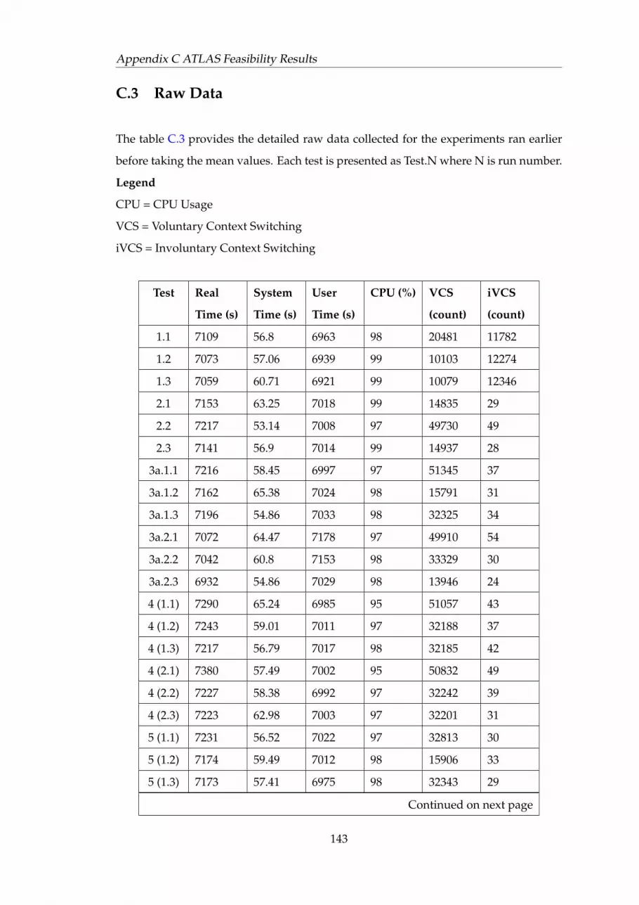
Appendix C ATLAS Feasibility Results
C.3 Raw Data
The table C.3 provides the detailed raw data collected for the experiments ran earlier
before taking the mean values. Each test is presented as Test.N where N is run number.
Legend
CPU = CPU Usage
VCS = Voluntary Context Switching
iVCS = Involuntary Context Switching
Test Real
Time (s)
System
Time (s)
User
Time (s)
CPU (%) VCS
(count)
iVCS
(count)
1.1 7109 56.8 6963 98 20481 11782
1.2 7073 57.06 6939 99 10103 12274
1.3 7059 60.71 6921 99 10079 12346
2.1 7153 63.25 7018 99 14835 29
2.2 7217 53.14 7008 97 49730 49
2.3 7141 56.9 7014 99 14937 28
3a.1.1 7216 58.45 6997 97 51345 37
3a.1.2 7162 65.38 7024 98 15791 31
3a.1.3 7196 54.86 7033 98 32325 34
3a.2.1 7072 64.47 7178 97 49910 54
3a.2.2 7042 60.8 7153 98 33329 30
3a.2.3 6932 54.86 7029 98 13946 24
4 (1.1) 7290 65.24 6985 95 51057 43
4 (1.2) 7243 59.01 7011 97 32188 37
4 (1.3) 7217 56.79 7017 98 32185 42
4 (2.1) 7380 57.49 7002 95 50832 49
4 (2.2) 7227 58.38 6992 97 32242 39
4 (2.3) 7223 62.98 7003 97 32201 31
5 (1.1) 7231 56.52 7022 97 32813 30
5 (1.2) 7174 59.49 7012 98 15906 33
5 (1.3) 7173 57.41 6975 98 32343 29
Continued on next page
143

Appendix C ATLAS Feasibility Results
continued from previous page
Test Real
Time (s)
System
Time (s)
User
Time (s)
CPU (%) VCS
(count)
iVCS
(count)
5 (2.1) 7180 56.58 6981 98 32708 39
5 (2.2) 7197 56.77 6992 98 15799 31
5 (2.3) 7206 57.52 7011 98 32355 35
6 (1.1) 7259 63.77 6953 97 50518 43
6 (1.2) 7196 53.68 6991 97 32322 25
6 (1.3) 7206 53.29 7002 97 32367 33
6 (2.1) 7284 54.48 6977 96 50213 41
6 (2.2) 7187 64.72 6966 97 32369 28
6 (2.3) 7196 61.73 6986 97 32441 40
7 (1.1) 7151 56.26 6948 97 32243 39
7 (1.2) 7144 58.95 6966 98 32537 39
7 (1.3) 7138 56.25 6989 98 32727 38
7 (2.1) 7175 63.21 7008 98 15768 33
7 (2.2) 7153 54.3 6965 98 29876 32
7 (2.3) 7161 57.22 6982 98 32806 35
8 (1.1) 8093 69.76 7602 94 95869 31
8 (1.2) 8097 69.04 7572 94 99222 33
8 (1.3) 7234 66.61 6901 96 101452 43
8 (2.1) 7627 59.3 6990 93 99769 37
8 (2.2) 7499 60.89 7010 95 65850 26
8 (2.3) 7723 67.66 6974 93 99724 35
8 (3.1) 8116 71 7604 94 94664 41
8 (3.2) 8103 68.75 7583 93 99310 44
8 (3.3) 8095 67.66 7583 94 96987 42
9 (1.1) 8002 66.16 7345 92 103603 47
9 (1.2) 7962 67.69 7370 93 98914 30
9 (1.3) 7905 69.61 7373 93 99244 39
9 (2.1) 8012 63.5 7339 92 103323 28
Continued on next page
144

Appendix C ATLAS Feasibility Results
continued from previous page
Test Real
Time (s)
System
Time (s)
User
Time (s)
CPU (%) VCS
(count)
iVCS
(count)
9 (2.2) 7890 69.66 7354 93 98770 41
9 (2.3) 7995 71.7 7376 93 98896 28
9 (3.1) 8043 64.87 7364 92 103304 59
9 (3.2) 7975 64.47 7391 93 98850 40
9 (3.3) 7956 64.34 7387 93 99040 30
10 (1.1) 14244 24.91 7034 49 98732 44
10 (1.2) 14105 21.76 7028 49 99290 42
10 (1.3) 10428 17.72 7020 50 99592 38
10 (2.1) 7324 59.73 6920 95 100670 31
10 (2.2) 7316 59.07 6925 95 100393 43
10 (2.3) 7286 57.55 6915 95 100580 33
10 (3.1) 7236 60.36 6911 96 101513 33
10 (3.2) 7214 55.91 6907 96 101489 28
10 (3.3) 7259 55.41 6946 96 101319 31
TABLE C.3: Raw Results for ATLAS Job Performance
145

Appendix C ATLAS Feasibility Results
C.4 Network Throughput Data
This data set represented in table C.4 are for each test configurations shown in table C.1.
Each test was run three times. Some tests were run in parallel virtual machines, thus
are represented in the following format Test (n) where n is the run number. For test
15 (1) and 15 (3), the transfer was done between two parallel virtual machines while in
test 15 (2), the data set was transfered from a physical machine.
Test Throughput (Mb/s) Time (s) Overhead (times X)11 62.8 66 0
12 (1) 8.8 349.1 2.912 (2) 8.4 365.7 2.912 (3) 7.9 379.3 313 (1) 8.3 370.1 313 (2) 8.4 65.7 2.913 (3) 8.3 370.1 314 (1) 7.8 94 3.214 (2) 8.4 64.3 2.814 (3) 9.3 329.1 2.7
15 (1.V) 6.4 480 3.915 (2) 15.8 194.4 1.7
15 (3.V) 6.6 467.8 3.8
TABLE C.4: Network throughput for ATLAS jobs running in virtual machines
146

Appendix D
PanDA Pilot Code
This appendix lists the code snippets from the selected sections of the PanDA pilot
code discussed in chapter 5, and which are relevant to the work done in this thesis. The
complete code base for the PanDA pilot is more than 100,000 lines. The PanDA pilot
application was developed in Python1 programming language by ATLAS experiment
collaboration.
D.1 Core Pilot Application
As described in section 5.1, PanDA pilot application have two major execution com-
ponents; pilotJob daemon script that initializes job, prepare the environment and is
responsible for cleanup operation, and runJob script that actually executes the job. In
this section, parts of pilotJob are elaborated which have been expanded to integrate
virtualization in to it.
D.1.1 Status Parameters
Panda pilot daemon, or more technically speaking pilotJob script, has number of
initial configuration parameters to enable proper execution of the job. To enable vir-
tualization, new parameters has to be added so that logical volume manager (LVM)
1Python Project, http://www.python.org
147

Appendix D PanDA Pilot Code
could create, mount, and remove partitions in the disk. In the modified version, job is
executed in the logical volume partitions.
These parameters include; virtualmachine - to boolean switch to determine the
mode of execution whether virtual or physical; vmstatus - to pass the job status infor-
mation back to the pilot job daemon from the runJob script; volumeGroup - where
the LVM partitions will be created; vmRoot - root partition for the job; vmSwap - the
swap partition needed for the virtual machine and finally jobMountWorkDir which
would be mount point used to configure the partition for each job in the initialization
phase.
12 # Will be set to True for virtual machine usage3 virtualmachine = True4 # To keep track of the virtual machine status5 vmstatus = ""6 volumeGroup = ""7 vmRoot = ""8 vmSwap = ""9 jobMountWorkdir = ""
D.1.2 Input Parameters
During it’s standard execution in physical machine, pilot job daemon labels the execu-
tion disk path as workdir along side other parameters to manage the debug level, site
information and proxy access check for authorization. To redirect the execution to the
virtual machine, additional parameters such as virtualmachine switch, jobMountWorkDir
mount point and insideVmWorkDir path needed for runJob script is added (see line
14 and 15).
12 """input arguments for the runJob script when executing3 in the virtual machine."""45 jobargs = [pyexe, "%s/runJob.py" % (jobDic["prod"][1].workdir),6 "-a", thisSite.appdir, "-d", jobDic["prod"][1].workdir,7 "-l", pilot_initdir, "-q", thisSite.dq2url,8 "-p", str(monthread.port),9 "-s", thisSite.sitename, "-o", thisSite.workdir,
10 "-m", str(multiTaskFlag),11 "-i", jobDic["prod"][1].tarFileGuid, "-b", str(debugLevel),12 "-t", str(proxycheckFlag),"-k", pUtil.getPilotlogFilename(),13 "-x", str(stageinTries), "-v", str(testLevel),14 "-c", str(virtualmachine), "-f", aJob.insideVmWorkdir,15 "-e", jobMountWorkdir]
148

Appendix D PanDA Pilot Code
D.1.3 Staging-In
During the staging-in phase when all the job configuration and initial data needed to
start the job is downloaded, a check was introduced to determine whether the execution
is going to follow in physical machine or virtual machine. Since virtualmachine
switch already redirected initial setup of the job directories in the LVM partition, a
simple check (at line 4) such as whether standard work directories path are created or
not was sufficient. If they are not present, then it’s assumed by the daemon that the
job will be running in the virtual machine and internal configuration parameters are
configured accordingly (see line 14).
Work directory paths are created using job ID name in the pre-defined disk space in the
worker node.
1 """if the job is running in the physical node, then follow2 the standard work directory path. """34 if os.path.isdir(jobDic["prod"][1].workdir):5 # copy all python files to workdir6 tolog("Staging in python modules to:7 %s" % (jobDic["prod"][1].workdir))8 pUtil.stageInPyModules(thisSite.workdir,9 jobDic["prod"][1].workdir)
10 else:1112 """ if the job is to be executed in the virtual machine,13 then use the virtual partition. """14 tolog("Staging in python modules to: %s" % (jobMountWorkdir))15 pUtil.stageInPyModules(thisSite.workdir, jobMountWorkdir)
D.1.4 Clean-up Phase
Once the job execution have either finished executing the job or the job has failed, then
it sends the message to the pilot daemon to trigger the cleanup operation. The pilot
daemon first follows it standard procedure to upload any logs or results to the grid,
then removes the LVM partition (line 3) and continues with removing all the pilot’s
own python scripts downloaded on the worker node host machine during the start-up
phase (line 5- 12).
1 def cleanup(job, rf=None):2 """ cleanup function """3 vmRemoveMountPoint(jobMountWorkdir)4
149

Appendix D PanDA Pilot Code
5 # clean up the pilot wrapper modules6 pUtil.removePyModules(job.workdir)78 if os.path.isdir(job.workdir):9 os.chdir(job.workdir)
10 # remove input files from the job workdir11 remFiles = job.inFiles12 tolog("Payload cleanup has finished")
D.2 RunJob Pilot Application
The runJob script is the main execution engine that executes the job, and in this section
the modification made to its code are highlighted.
D.2.1 Job Execution Phase
Pilot job daemon starts the execution engine by invoking a separate python interpreter
and passes in the input variables via the shell. But to start the execution engine in the
virtual machine once it starts up, this process has to be modified. The adopted solution
was to dump the input parameters into a data file which will be loaded by the execution
engine at the start up (see line 8).
If the execution is physical (line 10), then standard execution path will be followed.
If the execution is virtual machine based (line 21), then execution engine forks a child
process to send period TCP message to the pilot daemon and subsequently to the server
(line 25-36).
1 # main process starts here2 if __name__ == "__main__":34 # argument parsing phase begins to start job execution5 jobSite = Site.Site()6 jobSite.setSiteInfo(argParser(sys.argv[1:]))78 filename = "%s/vmRunJobDataFile.dat" % (jobSite.workdir)9
10 if not virtualmachine and os.path.exists(filename):11 from pickle import load1213 try:14 tolog("Trying to open %s" % (filename))15 vmRunJobDataFile = open("%s" % (filename), "r")16 jobargs = load(vmRunJobDataFile)
150

Appendix D PanDA Pilot Code
1718 except Exception, e:19 tolog("!!FAILED!!2999!! Could not import jobargs from:20 %s, %s" % (filename, str(e)))21 else:22 tolog("Got: %s" % (jobargs))23 pid_1 = os.fork()2425 if pid_1: # parent26 tolog("Parent process")27 else: # child28 tolog("Child process")29 _i = 030 while _i < 5:31 tolog("Updating pilot server:32 %s:%d" % (pilotserver, pilotport))33 job.result[0] = 'vmrunning'34 rt, rv = RunJobUtilities.updatePilotServer35 (job, pilotserver, pilotport)36 time.sleep(60)
D.2.2 Status Update
During the course of it’s execution, pilot daemon monitors certain file paths to see
whether the execution have finished or not. Since this long was feasible in the virtual
machine, because during the virtual machine based execution LVM partition is not
accessible by the host OS where the pilot daemon resides. Therefore, a TCP based
status update system was added where job execution engine update the pilot daemon
about the job progress.
This code provides one example where if the job fails, then the execution sends a TCP
message using utilities function to update the pilot server and daemon (see line 11-12).
1 def failJob(transExitCode, pilotExitCode, job, pilotserver,2 pilotport, ins=None, pilotErrorDiag=None, docleanup=True):34 """ set the fail code and exit """5 job.setState(["failed", transExitCode, pilotExitCode])67 if pilotErrorDiag:8 job.pilotErrorDiag = pilotErrorDiag9 tolog("Will now update pilot server")
10 #virtualization code block11 rt, rv = RunJobUtilities.updatePilotServer(job,12 pilotserver, pilotport, final=True)1314 if docleanup:15 sysExit(job)
151
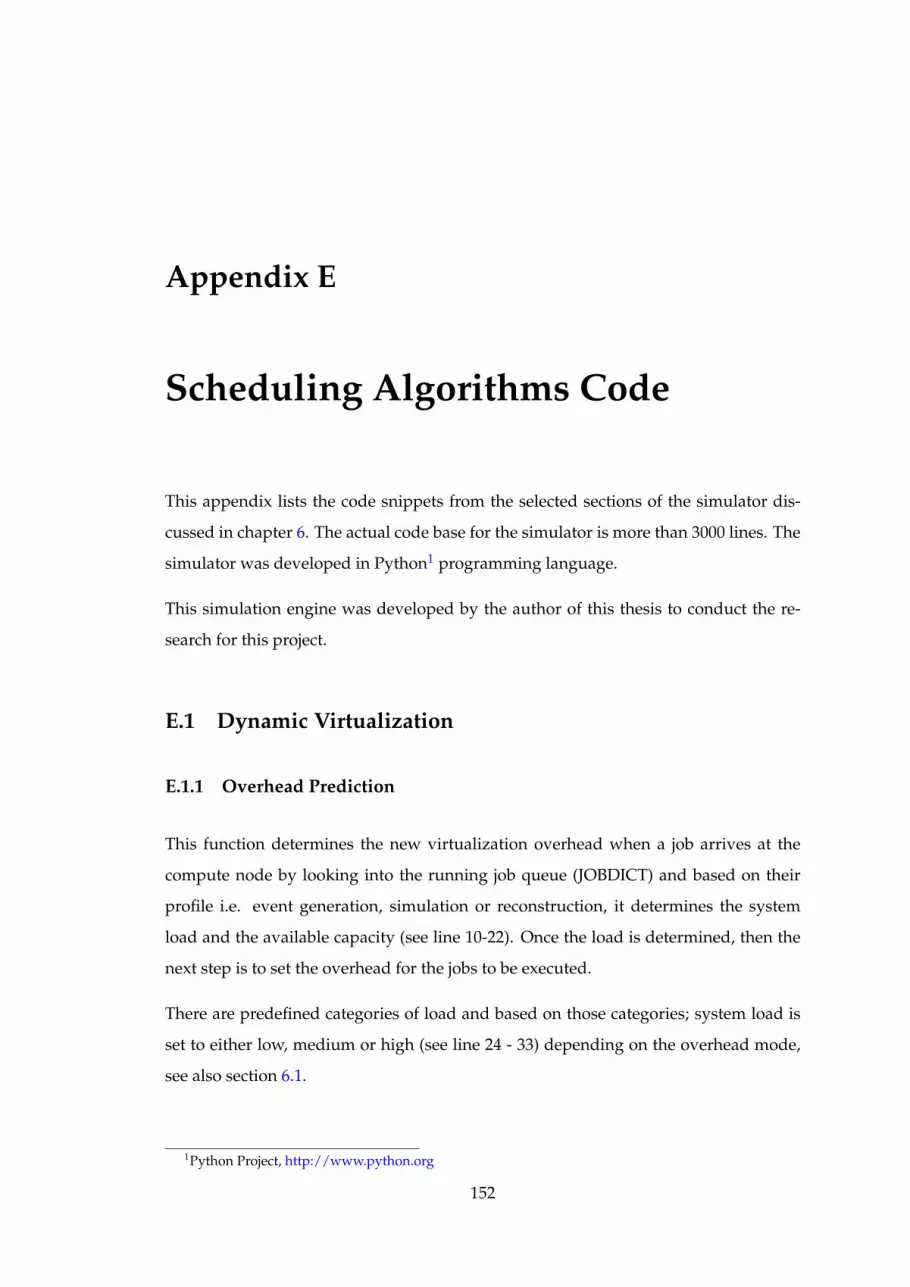
Appendix E
Scheduling Algorithms Code
This appendix lists the code snippets from the selected sections of the simulator dis-
cussed in chapter 6. The actual code base for the simulator is more than 3000 lines. The
simulator was developed in Python1 programming language.
This simulation engine was developed by the author of this thesis to conduct the re-
search for this project.
E.1 Dynamic Virtualization
E.1.1 Overhead Prediction
This function determines the new virtualization overhead when a job arrives at the
compute node by looking into the running job queue (JOBDICT) and based on their
profile i.e. event generation, simulation or reconstruction, it determines the system
load and the available capacity (see line 10-22). Once the load is determined, then the
next step is to set the overhead for the jobs to be executed.
There are predefined categories of load and based on those categories; system load is
set to either low, medium or high (see line 24 - 33) depending on the overhead mode,
see also section 6.1.
1Python Project, http://www.python.org
152

Appendix E Scheduling Algorithms Code
1 def getNextVO():2 try:3 if MODE ==VIRTUAL:4 eve=05 rec=06 sim=07 getcontext().prec =38 # gather running job distribution9 iter = JOBDICT.__iter__()
10 for each in iter:11 if each['type'] == EVE and each['status'] == "running":12 eve +=0.513 elif each ['type'] == SIM and each['status'] == "running":14 sim +=115 elif each['type'] == REC and each['status'] == "running":16 rec += 1.517 #total number of jobs18 numVM = len(JOBDICT)19 capacity = MEMORY + CPU20 vmLoadSum = eve + sim + rec21 # load = vmLoadSum / numVM22 LOAD=load = vmLoadSum * numVM / capacity2324 if VO_MODE == VO_DYNAMIC:25 # set the VO dynamically26 if load < 1 :27 return VO_LOW28 elif load == 1:29 return VO_MED30 elif load > 1:31 return VO_HIGH32 elif VO_MODE==VO_FLAT:33 return VO_HIGH34 except Exception, e:35 msg = "ERROR: getNextVO() -> [Exception: %s]" % (e)36 printMessage(msg, B_SYSTEM_MSG)
153

Appendix E Scheduling Algorithms Code
E.1.2 Real Job Progress
In each cycle of the virtualization, there is a generated overhead either low, medium
and high. If the execution mode is set to virtual (line 4-6), then a real progress offset
is calculated which is then deduced from the job duration to represent job progressing
over time.
1 def updateDynamicVO():2 # update the VO OFFSET3 try:4 if MODE == VIRTUAL:5 FREQ_VO = VO * FREQ / 1006 FREQ_OFFSET = FREQ - FREQ_VO7 else:8 FREQ_OFFSET = FREQ9 FREQ_VO = 0
10 except Exception, e:11 msg = "ERROR: FREQ_OFFSET calculation failed > [%s]" % (e)12 printMessage(msg, B_BASE_MSG)
E.1.3 Job Deadline Validation
Once a new job arrives, before it’s started; the job duration for running jobs have to be
updated to reflect the new overhead impact. This function first get the new overhead
(line 9) and if it’s greater than the previous one (which could be highest), than it checks
the duration remaining of all the jobs in the running queue (line 15-22 ). If any job
appears to miss their deadline because of this new job (line 29-42) then the new job
is terminated prematurely. This is to increase system performance by minimizing the
impact on the existing jobs which might have been running for longer and to give them
higher chance of success.
1 def getNextVOImpact():2 #this function should validate all current deadline3 #commitment and if existing commitments could4 #not be fullfilled, then don't next job so return5 #False(no next job)/True(yes, next job)67 boolDecision = False8 try:9 VO_NEXT = getNextVO()
10 newOverhead = VO_NEXT * FREQ / 10011 # this is the real progress per slot for the job duration12 #by removing the virtualization's slow rate13 realProgressPerSlot = FREQ - newOverhead14
154

Appendix E Scheduling Algorithms Code
15 if VO_NEXT > VO:16 jobDuration = []17 iter = JOBDICT.__iter__()18 for each in iter:19 # check against the jobs whose status is20 #finished so not to measure against their deadlines21 if each['status'] != "finished":22 jobDuration.append(each['duration'])23 #sort the durations24 jobDuration.sort()2526 #since we can only sort on single values not27 #duration:deadline, so we need to re-iterate28 #over JOBDICTIONARY to get the deadline29 iter = JOBDICT.__iter__()30 for each in iter:31 # check against the shortest job as this32 #is the determining factor because upon33 #it's completion another job slot would34 #be available and there would be a different35 #VO_NEXT36 if each['status'] != "finished":37 newJobDuration =38 each['duration'] * newOverhead39 if newJobDuration > each['deadline']:40 boolDecision=False41 else:42 boolDecision=True43 except Exception, e:44 msg= "ERROR: getNextVOImpact() -> [Exception: %s]" % (e)45 printMessage(msg, B_BASE_MSG)46 return boolDecision
E.2 Adaptive Algorithms
The computational code used in the scheduling algorithms is discussed in this section.
E.2.1 Failure Rate Calculation
As discussed in section 4.2, the failure rate is calculated using exponential smoothening
method where parameter α is used to determine the success rate. In the simulator, each
job could either finish successfully (success boolean set to true) or fail (success boolean
set to false). At the end of each job, calculate success rate function is called and based on
the input boolean, a local variable is either set to 1 or -1 (line 9-12). Once the system
155

Appendix E Scheduling Algorithms Code
have gone through the first 1000 jobs to warm up, then success rate is calculated using
equation 4.9 (line 19-24).
Finally, failure rate is calculated (line 32-35).
1 def calculate_success_rate(success):2 # one time alpha and success rate is already3 #defined at the initialization of the script4 #x_mode_value is to use one of success_rate calculation mechanisms56 try:7 if X_Mode_Value==1:8 # recalculate alpha if it could be done9 if success:
10 success_var=111 else:12 success_var=-11314 # training switch added for first 1000 iterations,15 #the code calculate division method to calculate16 #the success rate and after it17 # uses digital integrator using alpha as division18 #operation of large numbers becomes a computational issue19 if stage_1_count > 1000:20 # inegrating and calculating the success rate21 success_rate = success_rate*(1-ALPHA) + success_var*ALPHA22 else:23 stage_1_count +=124 success_rate = TOTAL_LEASE_SUC/TOTAL_LEASED_JOBS25 except Exception, e:26 msg="ERROR: calculate_success_rate() -> Exception: [%s]" %(e)27 printMessage(msg, B_BASE_MSG)2829 def get_failure_rate():30 calculate_success_rate()31 failure_rate = 1 - success_rate32 return failure_rate
E.2.2 x Threshold Adaptation
Once the failure rate have been calculated (line 18), the next step is to update the
XThresh. To avoid prematurely changing the threshold or changing it too fast, there
is delay mechanism built in. If the failed numbers of jobs are greater than failed job
threshold since the last time XThresh was altered, only then adaptive algorithm gets ac-
tivated (line 23-26). Once the algorithm is in this part of code (line 31 -35), then XThresh
is either incremented or decremented using ∆x parameter (see section 4.2.4). Once the
adaptation have taken place, then minimum and maximum x values are checked to
156
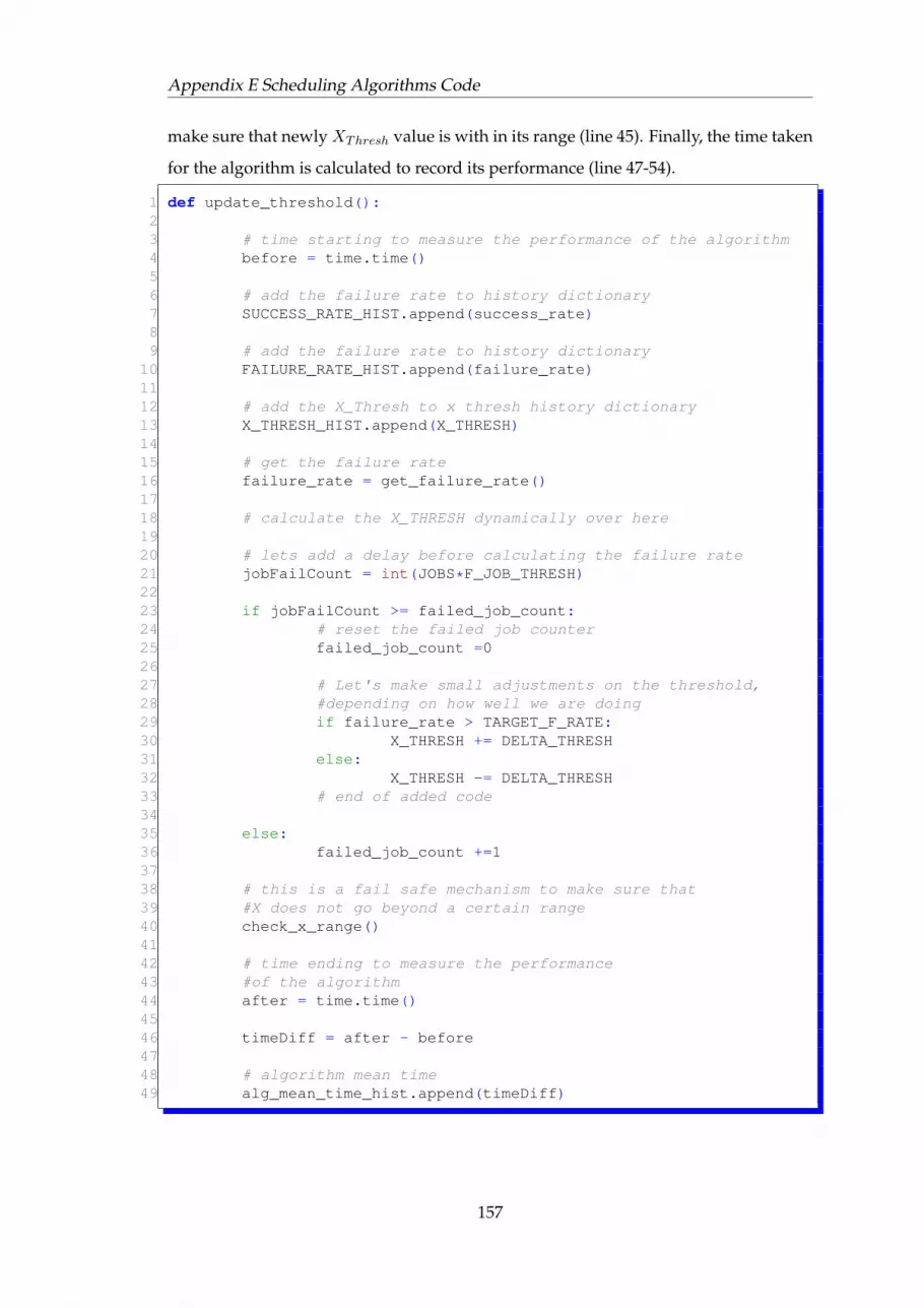
Appendix E Scheduling Algorithms Code
make sure that newly XThresh value is with in its range (line 45). Finally, the time taken
for the algorithm is calculated to record its performance (line 47-54).
1 def update_threshold():23 # time starting to measure the performance of the algorithm4 before = time.time()56 # add the failure rate to history dictionary7 SUCCESS_RATE_HIST.append(success_rate)89 # add the failure rate to history dictionary
10 FAILURE_RATE_HIST.append(failure_rate)1112 # add the X_Thresh to x thresh history dictionary13 X_THRESH_HIST.append(X_THRESH)1415 # get the failure rate16 failure_rate = get_failure_rate()1718 # calculate the X_THRESH dynamically over here1920 # lets add a delay before calculating the failure rate21 jobFailCount = int(JOBS*F_JOB_THRESH)2223 if jobFailCount >= failed_job_count:24 # reset the failed job counter25 failed_job_count =02627 # Let's make small adjustments on the threshold,28 #depending on how well we are doing29 if failure_rate > TARGET_F_RATE:30 X_THRESH += DELTA_THRESH31 else:32 X_THRESH -= DELTA_THRESH33 # end of added code3435 else:36 failed_job_count +=13738 # this is a fail safe mechanism to make sure that39 #X does not go beyond a certain range40 check_x_range()4142 # time ending to measure the performance43 #of the algorithm44 after = time.time()4546 timeDiff = after - before4748 # algorithm mean time49 alg_mean_time_hist.append(timeDiff)
157

Appendix E Scheduling Algorithms Code
E.2.3 Statistical Determination
The probabilistic algorithm uses cumulative distribution functions. In our results,XThresh
values which succeeded after they first appeared to have missed their deadline are
recorded in an array named X SUC HIST. This array which is our sample space is
passed to a python function histogram from the Scipy2 and gets a discreet data dis-
tribution of the data points in a histogram (line 2). This histogram is then normalized
and used by the Scipy cumsum function to return a cumulative distribution (line 8-9).
Then the XThresh value for probability higher than 0.5 is determined (line 11).
In get xi function, line 16-18 are standard methods to get to value of XThresh which
corresponds to the input probability. For more details, see Scipy documentation. Once
a value for XThresh is available, then if it falls out side the range of 50 then its sets to
minimum XThresh value otherwise its set to XThresh and used as a validation condition
either to let the job continue or not.
It should be noted that the value 50 passed to histogram function (line 2) and 49 (line 19)
represents the maximum number of probability data points. Generally, this value was
around 25 in the simulated system which is just in the range, and thus arrived through
experimentation.
1 def get_cdf():2 px,xe = histogram(X_SUC_HIST, 50, normed=True)34 x1=xe[0:-1] # left edges5 x2=xe[1:] # right edges6 x=0.5*(x1+x2)78 px=px/sum(px) # normalize, so that sum(px)=19 PX = cumsum(px) # CDF
1011 x_i = get_xi(PX, x, 0.5)12 print 'x_i=%g' % x_i1314 def get_xi(PX, x, prob):15 global X_THRESH16 indx = where(PX<prob)17 index = max(indx[0]+1)18 x_thr = x[index]19 if index > 49 or indx < 0:20 X_THRESH=0.121 else:22 X_THRESH=x_thr23 return X_THRESH
2Scipy Libraryhttp://www.scipy.org
158

Appendix E Scheduling Algorithms Code
E.2.4 Probabilistic x Adaptation
To determine the XThresh using the statistical techniques is identical to function de-
scribed in section E.2.2 except that rather than using ∆x and alpha α values, it call get
cdf function (line 32).
1 def update_threshold_prob():23 # time the performance of the algorithm4 before = time.time()56 # added code78 # add the failure rate to history dictionary9 SUCCESS_RATE_HIST.append(success_rate)
1011 # add the failure rate to history dictionary12 FAILURE_RATE_HIST.append(failure_rate)1314 # add the X_Thresh to x thresh history dictionary15 X_THRESH_HIST.append(X_THRESH)1617 # get the failure rate18 failure_rate = get_failure_rate()1920 # calculate the X_THRESH dynamically over here2122 # lets add a delay before calculating the failure rate23 jobFailCount = int(JOBS*F_JOB_THRESH)2425 if jobFailCount >= failed_job_count:26 # reset the failed job counter27 failed_job_count =02829 # Let's make small adjustments on the threshold,30 #depending on how well we are doing31 if failure_rate > TARGET_F_RATE:32 get_cdf()33 else:34 failed_job_count +=13536 # this is a fail safe mechanism to make sure37 #that X does not go beyond a certain range38 check_x_range()3940 # time ending to measure the performance41 #of the algorithm42 after = time.time()4344 timeDiff = after - before4546 # algorithm mean time47 alg_mean_time_hist.append(timeDiff)
159

Appendix F
Resource Utilization
F.1 Results
This section provides more detailed results gathered during the training phase to fur-
ther study the impact of various configuration of resource ratio (primarily number of
GB memory per CPU core) in the system. The results are discussed in the following
subsections for each resource ratio.
F.1.1 CPU to Memory ratio: 1 to 1
In this configuration, the job success rate was around 70% with job termination rate
fluctuating between 25%-43% with dead line miss rate to be around 5% as show in
F.1. The higher rate of job termination is due to the fact that there are more jobs with
higher resource requirements than the available on the machine. This is key factor in
determining what should be the optimal resource configuration for compute node to
avoid jobs being terminated for ATLAS experiment.
Where as memory and CPU utilization rate is concerned, as shown in figure F.2(a) and
F.2(b), the utilization is not optimal either since a significantly large number of jobs gets
terminated even before starting.
160

Appendix F Resource Utilization
0 50 100 150 200 250 300 350 400 450Simulation Time Unit
0.0
0.1
0.2
0.3
0.4
0.5
0.6
0.7
0.8
Rate
Resource Resolution Performance (ratio 1:1)
termination rate
deadline miss rate
success rate
FIGURE F.1: Job Success, Termination and Deadline failure rate for CPU:Memory ratio1:1
161

Appendix F Resource Utilization
0 50 100 150 200 250 300 350 400 450Simulation Time Unit
0.0
0.2
0.4
0.6
0.8
1.0
Utili
zatio
n Ra
te
CPU Utilization
cpu slot 1cpu slot 2cpu slot 3cpu slot 4
(a) CPU Utilization rate for CPU:Memory ratio 1:1
0 50 100 150 200 250 300 350 400 450Simulation Time Unit
0.3
0.4
0.5
0.6
0.7
0.8
0.9
1.0
Utili
zatio
n Ra
te
Memory Utilization
memory slot 1memory slot 2memory slot 3memory slot 4
(b) Memory Utilization rate for CPU:Memory ratio 1:1
FIGURE F.2: CPU and Memory utilization rate for CPU:Memory ratio 1:1
162

Appendix F Resource Utilization
F.1.2 CPU to Memory ratio: 1 to 1.5
When the resource configuration was set to 1:1.5, we observe that job termination rate
drops significantly to 5% from previous configuration, and showing an improvement
of around 20%to 30% while job success rate reaches an average of 85% with no visible
impact on job deadline rate.
0 100 200 300 400 500Simulation Time Unit
0.0
0.2
0.4
0.6
0.8
1.0
Rate
Resource Resolution Performance (ratio 1:1.5)
termination rate
deadline miss rate
success rate
FIGURE F.3: Job Success, Termination and Deadline failure rate for CPU:Memory ratio1:1.5
Increasing the available memory in the system also increases over all system utilization
rate where CPU 2 and 3 showing higher utilization rate, as compared to figure F.2(a),
since more jobs get a chance to run rather being terminated. The same principal applies
to memory utilization rate as show in figure F.4(b).
163

Appendix F Resource Utilization
0 100 200 300 400 500Simulation Time Unit
0.1
0.2
0.3
0.4
0.5
0.6
0.7
0.8
0.9
1.0
Utili
zatio
n Ra
te
CPU Utilization
cpu slot 1cpu slot 2cpu slot 3cpu slot 4
(a) CPU Utilization rate for CPU:Memory ratio 1:1.5
0 100 200 300 400 500Simulation Time Unit
0.0
0.2
0.4
0.6
0.8
1.0
Utili
zatio
n Ra
te
Memory Utilization
memory slot 1memory slot 2memory slot 3memory slot 4memory slot 5memory slot 6
(b) Memory Utilization rate for CPU:Memory ratio 1:1.5
FIGURE F.4: CPU and Memory utilization rate for CPU:Memory ratio 1:1.5
164

Appendix F Resource Utilization
F.1.3 CPU to Memory ratio: 1 to 2
With ratio set to 2, it was observed that job termination almost disappears suggesting
that this might be perhaps the optimal resource configuration ATLAS, and LHC jobs in
general since no job is deprived of available resources with job success rate higher than
80%.
0 50 100 150 200 250 300 350Simulation Time Unit
0.0
0.2
0.4
0.6
0.8
1.0
Rate
Resource Resolution Performance (ratio 1:2)
termination rate
deadline miss rate
success rate
FIGURE F.5: Job Success, Termination and Deadline failure rate for CPU:Memory ratio1:2
Interestingly, the resource utilization rate slightly decrease from previous average of
70% for both CPU and Memory. In our view, this is a trade-off between slightly under
utilized resources with minimum and unnecessary job termination rate.
165

Appendix F Resource Utilization
0 50 100 150 200 250 300 350Simulation Time Unit
0.0
0.2
0.4
0.6
0.8
1.0
Utili
zatio
n Ra
te
CPU Utilization
cpu slot 1cpu slot 2cpu slot 3cpu slot 4
(a) CPU Utilization rate for CPU:Memory ratio 1:2
0 50 100 150 200 250 300 350Simulation Time Unit
0.0
0.2
0.4
0.6
0.8
1.0
Utili
zatio
n Ra
te
Memory Utilization
memory slot 1memory slot 2memory slot 3memory slot 4memory slot 5memory slot 6memory slot 7memory slot 8
(b) Memory Utilization rate for CPU:Memory ratio 1:2
FIGURE F.6: CPU and Memory utilization rate for CPU:Memory ratio 1:2
166

Appendix F Resource Utilization
F.1.4 CPU to Memory ratio: 1 to 3
The results for ratio 1:3 are similar to ratio 1:2 for job success rate and termination rate.
The resource utilization rate further decreases as compared to resource ratio of 1:2. As
a result, resource ratio for CPU to Memory was set to 1:12 for all experiments in the
steady phase.
0 50 100 150 200 250 300 350Simulation Time Unit
0.0
0.2
0.4
0.6
0.8
1.0
Rate
Resource Resolution Performance (ratio 1:3)
termination rate
deadline miss rate
success rate
FIGURE F.7: Job Success, Termination and Deadline failure rate for CPU:Memory ratio1:3
167

Appendix F Resource Utilization
0 50 100 150 200 250 300 350Simulation Time Unit
0.0
0.2
0.4
0.6
0.8
1.0
Utili
zatio
n Ra
te
Memory Utilization
memory slot 1memory slot 2memory slot 3memory slot 4memory slot 5memory slot 6memory slot 7memory slot 8memory slot 9memory slot 10memory slot 11memory slot 12
(a) CPU Utilization rate for CPU:Memory ratio 1:3
0 50 100 150 200 250 300 350Simulation Time Unit
0.0
0.2
0.4
0.6
0.8
1.0
Utili
zatio
n Ra
te
CPU Utilization
cpu slot 1cpu slot 2cpu slot 3cpu slot 4
(b) Memory Utilization rate for CPU:Memory ratio 1:3
FIGURE F.8: CPU and Memory utilization rate for CPU:Memory ratio 1:3
168
Appendix G
Alpha and Delta x Training
G.1 Training Results
G.1.1 α1=0.01
Since alpha α value is very small, the deadline miss rate increases initially and it takes
a while before adaptive algorithm responds. As shown in figure G.1(a) and G.1(b),
failure rate peaks between 20-40 simulation time units, and the XThresh value hits it
floor of 0.1 before being incremented to it’s upper ceiling value of 0.9.
G.1.2 α2=0.05
In this case, a higher alpha α value activates the algorithm faster and failure rate, as
seen in figure G.2(b), is brought down from 0.5 peak value to 0.2 with in 0-25 simulation
time units. The system better for over all global success rate and lower deadline miss
rate, see figure G.2(a).
G.1.3 α3=0.1
The results of alpha α value for 0.05 and 0.1 are very similar in terms of overall system
performance with slightly lower failure rate for the later configure but since the dead-
line miss rate is approximately the same, see figure G.3(a) and G.3(b), we selected 0.05
169

Appendix G Alpha and Delta x Training
0 100 200 300 400 500 600Simulation Time Unit
0.0
0.1
0.2
0.3
0.4
0.5
0.6
0.7
0.8
0.9
Rate
Global System Performance (alpha=0.01)
termination rate
deadline miss rate
success rate
(a) System Peformance
0 50 100 150 200 250 300 350 400Simulation Time Unit
0.0
0.1
0.2
0.3
0.4
0.5
0.6
0.7
0.8
0.9
Valu
e
Failure rate and X_Threshold evolution (Global success: 0.88) [delta_x:0.1, alpha:0.01, target_f_rate:0.25, overall_f_rate:0.169270833333]
Failure rateX Thresh
(b) X Threshold and Failure rate evolution
FIGURE G.1: Training Results for α1=0.01
170

Appendix G Alpha and Delta x Training
0 100 200 300 400 500 600Simulation Time Unit
0.0
0.2
0.4
0.6
0.8
1.0
Rate
Global System Performance (alpha=0.05)
termination rate
deadline miss rate
success rate
(a) System Peformance
0 50 100 150 200 250 300 350 400Simulation Time Unit
0.0
0.1
0.2
0.3
0.4
0.5
0.6
0.7
0.8
0.9
Valu
e
Failure rate and X_Threshold evolution (Global success: 0.927) [delta_x:0.1, alpha:0.05, target_f_rate:0.25, overall_f_rate:0.15710723192]
Failure rateX Thresh
(b) X Threshold and Failure rate evolution
FIGURE G.2: Training Results for α2=0.05
171

Appendix G Alpha and Delta x Training
as optimal value since under higher failure rate it will prevent x threshold to step up
or down slower to make sure that system doesn’t change its long term behavior due to
short-term and temporary execution conditions e.g. lots of similar jobs suddenly start
to fail for reasons external to system such as unable to access the grid storage sites.
0 100 200 300 400 500 600Simulation Time Unit
0.0
0.2
0.4
0.6
0.8
1.0
Rate
Global System Performance (alpha=0.1)
termination rate
deadline miss rate
success rate
(a) System Peformance
0 50 100 150 200 250 300 350 400 450Simulation Time Unit
0.0
0.1
0.2
0.3
0.4
0.5
0.6
0.7
0.8
0.9
Valu
e
Failure rate and X_Threshold evolution (Global success: 0.927) [delta_x:0.1, alpha:0.1, target_f_rate:0.25, overall_f_rate:0.14691943128]
Failure rateX Thresh
(b) X Threshold and Failure rate evolution
FIGURE G.3: Training Results for α3=0.1
172

Appendix G Alpha and Delta x Training
G.1.4 ∆x1=0.05
Experimentation showed that ∆x1=0.05 has the least performance and highest failure
rate among the three different ∆x configurations. This is due to the fact that a small
delta leads to smaller step incremental or decremental changes in XThresh value when
the failure rate goes up and down, and thus always lagging behind the failure rate
curve. See figure G.4.
0 100 200 300 400 500 600Simulation Time Unit
0.0
0.2
0.4
0.6
0.8
1.0
Rate
Global System Performance (delta=0.05)
termination rate
deadline miss rate
success rate
(a) System Peformance
0 50 100 150 200 250 300 350 400 450Simulation Time Unit
0.0
0.2
0.4
0.6
0.8
1.0
Valu
e
Failure rate and X_Threshold evolution (Global success: 0.917) [delta_x:0.05, alpha:0.05, target_f_rate:0.25, overall_f_rate:0.165919282511]
Failure rateX Thresh
(b) X Threshold and Failure rate evolution
FIGURE G.4: Training Results for ∆x=0.05
173

Appendix G Alpha and Delta x Training
G.1.5 ∆x2=0.1
This outperformed all the other test configurations with the highest global success rate
and lowest failure rate, see figure G.5. This proves our hypothesis that any successful
∆x and alpha α combination be apart by a factor of [5 -10].
0 100 200 300 400 500 600Simulation Time Unit
0.0
0.2
0.4
0.6
0.8
1.0
Rate
Global System Performance (delta=0.1)
termination rate
deadline miss rate
success rate
(a) System Peformance
0 50 100 150 200 250 300 350 400 450Simulation Time Unit
0.0
0.1
0.2
0.3
0.4
0.5
0.6
0.7
0.8
0.9
Valu
e
Failure rate and X_Threshold evolution (Global success: 0.942) [delta_x:0.1, alpha:0.05, target_f_rate:0.25, overall_f_rate:0.113689095128]
Failure rateX Thresh
(b) X Threshold and Failure rate evolution
FIGURE G.5: Training Results for ∆x=0.1
174

Appendix G Alpha and Delta x Training
G.1.6 ∆x3=0.2
This configuration performed slightly better than ∆x1 while the failure rate evolution
is very similar of that ∆x2 configuration. This may be because ∆x3 is perhaps too large
and it starts getting of failure rate curve.
0 100 200 300 400 500Simulation Time Unit
0.0
0.2
0.4
0.6
0.8
1.0
Rate
Global System Performance (delta=0.2)
termination rate
deadline miss rate
success rate
(a) System Peformance
0 100 200 300 400 500Simulation Time Unit
0.0
0.1
0.2
0.3
0.4
0.5
0.6
0.7
0.8
0.9
Valu
e
Failure rate and X_Threshold evolution (Global success: 0.926) [delta_x:0.2, alpha:0.05, target_f_rate:0.25, overall_f_rate:0.149450549451]
Failure rateX Thresh
(b) X Threshold and Failure rate evolution
FIGURE G.6: Training Results for ∆x=0.2
175

Bibliography
[1] O. Khalid, T. Koeckerbauer, D. Shiyachki, A. Unterkircher, and M. Schulz. The
vgrid project. Enabling Grids for E-Science, 2007. iv, 83
[2] O. Khalid, P. Nillson, M. Schulz, and K. Keahey. Enabling virtual panda pilot for
atlas. Enabling Grids for E-Science, 2008. iv, 86
[3] O. Khalid, P. Nillson, M. Schulz, and K. Keahey. Executing atlas jobs in virtual
machines. Computing in High Energy Physics, 2009. iv
[4] O. Khalid, R. Anthony, P. Nilsson, K. Keahey, M. Schulz, K. Parrott, and
M. Petridis. Enabling and optimizing pilot jobs using xen virtual machines for
hpc grid applications. In Proceedings of the 3rd IEEE/ACM International Workshop
on Virtualization Technologies in Distributed Computing, VTDC’09, pages 1–8, June
2009. doi: http://doi.acm.org/10.1145/1555336.1555338. iv, 81
[5] O. Khalid, I. Maljevic, R. Anthony, M. Petridis, K. Parrott, and M. Schulz. Dy-
namic scheduling of virtual machines running hpc workloads in scientific grids.
In Proceedings of 3rd International Conference on New Technologies, Mobility and Se-
curity, NTMS’09, pages 1 –5, Dec. 2009. doi: http://dx.doi.org/10.1109/NTMS.
2009.5384725. iv
[6] O. Khalid, I. Maljevic, R. Anthony, M. Petridis, K. Parrott, and M. Schulz. Dead-
line aware virtual machine scheduler for scientific grids and cloud computing. In
Proceeding of 24th IEEE International Conference of Advance Information Networking
and Applications, April 2010. iv
[7] I. Foster and C. Kesselman. The Grid: Blueprint for New Infrastructure. Morgan
Kaufmann Publishers, 1999. 1, 11, 19
176

Bibliography
[8] G. F. Pfister. In Search of Clusters. Prentice Hall, Upper Saddle River, USA, 3rd
edition, 1998. 1
[9] R. Buyya. High Performance Cluster Computing: Architecture and Systems, volume 1.
Prentice Hall, Upper Saddle River, USA, 1999. 1
[10] R. George. Desktop virtualization. Information Week Magzine, Aug 2009. 1
[11] G. Haff. I/o virtualization’s competing forms. CNet News, Oct 2009. URL http:
//news.cnet.com/8301-13556_3-10381070-61.html. 1
[12] K. Keahey, K. Doering, and I. Foster. From sandbox to playground: Dynamic
virtual environments in the grid. 5th International Workshop in Grid Computing,
2004. 2
[13] J. Barr. Grid computing done right. HPC Wire, Nov 2009. URL
http://www.hpcwire.com/specialfeatures/cloud_computing/
features/Grid-Computing-Done-Right-68597302.html. 2, 42
[14] R. Figueiredo, P. Dinda, and J. Fortes. A case for grid computing on virtual ma-
chines. 23rd International Conference on Distributed Computer Systems, 2003. 2, 12
[15] Accessed on Oct 2009 Enabling European Grids for E-Science. Glite grid middle-
ware. URL http://www.glite-eu.org. 7
[16] M. Tadashi and ATLAS Collaboration. Panda: Distributed production and dis-
tributed analysis system for atlas. J.Phys.Conf.Ser., 119(062036):4, 2008. 7, 25
[17] R. J. Creasy. The origin of the vm/370 time-sharing system. IBM Journal of Re-
search and Development, 25(5):483–490, 1981. ISSN 0018-8646. 11
[18] R. P. Goldberg. Survey of virtual machine research. IEEE Computer Magzine, 7(6):
34–45, 1974. 11
[19] B. Sotomayor. Resource management model for vm based virtual workspaces.
Master thesis, University of Chicago, 2007. URL http://workspace.globus.
org/papers/Workspace_Resource_Mgmt_Sotomayor_Masters.pdf. 11
[20] A. Butt. Grid-computing portals and security issues. In Journal of Parallel and
Distributed Computing, 2003. 11
177

Bibliography
[21] B. P. Miller, M. Christodorescu, R. Iverson, T. Kosar, A. Mirgorodskii, and
F. Popovici. Playing inside the black box: Using dynamic instrumentation to
create security holes. Parallel Process Letters, 11(2,3):267–280, 2001. 11
[22] B. Calder, A. A. Chien, S. Elbert, and K. Bhatia. Entropia: architecture and perfor-
mance of an enterprise desktop grid system. In Journal of Parallel and Distributed
Computing, 63(5):597–610, 2003. 11
[23] P. H. Kamp and R. N. M. Watson. Jails: Confining the omnipotent root. FreeBSD
project, 2000. URL http://phk.freebsd.dk/pubs/sane2000-jail.pdf.
11
[24] R. Uhlig, G.Neiger, D. Rodgers, A.L. Santoni, F.C.M. Martins, A.V. Anderson,
S.M. Bennett, A. Kagi, F.H. Leung, and L. Smith. Intel virtualization technology.
IEEE Computer Society Journal, 38(5):48–56, May 2005. 13, 14
[25] Xen hypervisor, accessed on oct 2009, . URL http://www.xen.org. 14, 16, 90
[26] J. Sugerman, G. Venkitachalam, and B-H. Lim. Virtualizing i/o devices on
vmware workstation’s hosted virtual machine monitor. In Proceedings of the Gen-
eral Track: 2002 USENIX Annual Technical Conference, pages 1–14, Berkeley, CA,
USA, 2001. USENIX Association. ISBN 1-880446-09-X. 14, 16
[27] Kernal-based virtual machine, accessed on oct 2009. URL www.linux-kvm.
org. 14
[28] Qemu processor emulator, accessed on oct 2009. URL http://www.qemu.org.
16
[29] S. Soltesz, H. Potzl, M. E. Fiuczynski, A. Bavier, and L. Peterson. Container-
based operating system virtualization: a scalable, high-performance alternative
to hypervisors. SIGOPS Oper. Syst. Rev., 41(3):275–287, 2007. ISSN 0163-5980. doi:
http://doi.acm.org/10.1145/1272998.1273025. 17
[30] D. Price and A. Tucker. Solaris zones: Operating system support for consolidat-
ing commercial workloads. In LISA ’04: Proceedings of the 18th USENIX conference
on System administration, pages 241–254, Berkeley, CA, USA, 2004. USENIX Asso-
ciation.
178

Bibliography
[31] Parallels. Virtuzzo containers, accessed on nov 2009. URL http://www.
parallels.com/eu/products/pvc45/.
[32] Linux Community. Linux vserver project, accessed on nov 2009. URL http:
//linux-vserver.org/. 17
[33] M. Rosenblum and T. Garfinkel. Virtual machine monitors: Current technology
and future trends. IEEE Computer Society Journal, 38(5), May 2005. 17
[34] I. Foster, C. Kesselman, and S. Tuecke. The anatomy of the grid: Enabling scal-
able virtual organizations. 1999. URL http://www.globus.org/alliance/
publications/papers/anatomy.pdf. 20
[35] S. Campana, M. Litmaath, and A. Sciaba. Technical report: Lcg middleware
overview. Technical report, CERN, Oct 2004. URL https://edms.cern.ch/
file/498079/0.1/LCG-mw.pdf. 21
[36] S.Burke, S. Campana, E. Lanciotti, P.M. Lorenzo, V. Miccio, C. Nater, R. San-
tinelli, and A. Sciaba. glite 3: User guide. Technical report, CERN, April 2009.
URL https://edms.cern.ch/file/722398/1.2/gLite-3-UserGuide.
pdf. 21
[37] ATLAS computing: Technical Design Report. Technical Design Report ATLAS.
CERN, Geneva, 2005. URL http://cdsweb.cern.ch/record/837738?ln=
en. revised version submitted on 2005-06-20 16:33:46. 24
[38] A. Tsaregorodtsev, M. Bargiotti, N. Brook, A. Casajus Ramo, G. Castellani,
P. Charpentier, C. Cioffi, J. Closier, R.G. Diaz, G. Kuznetsov, Y.Y. Li, R. Nandaku-
mar, S. Paterson, R. Santinelli, A.C. Smith, M. S. Miguelez, and S. G. Jimenez.
Dirac: A community grid solution. Conforence on Computing in High Energy
Physics (CHEP), 2007. URL https://twiki.cern.ch/twiki/pub/LHCb/
DiracProjectPage/DIRAC_CHEP07_mod5.pdf. 25
[39] P. Ruth, X. Jiang, D. Xu, and S. Goasguen. Virtual distributed environments in
a shared infrastructure. Computer, 38(5):63–69, 2005. ISSN 0018-9162. doi: http:
//dx.doi.org/10.1109/MC.2005.175. 29
179

Bibliography
[40] K. Keahey., I. Foster, T. Freeman, and X. Zhang. Virtual workspaces: Achieving
quality of service and quality of life in the grid. Sci. Program., 13(4):265–275, 2005.
ISSN 1058-9244. 31
[41] L. Grit, D. Irwin, A. Yumerefendi, and J. Chase. Virtual machine hosting for
networked clusters: Building the foundations for autonomic orchestration. In
VTDC ’06: Proceedings of the 2nd International Workshop on Virtualization Technology
in Distributed Computing, page 7, Washington, DC, USA, 2006. IEEE Computer
Society. ISBN 0-7695-2873-1. doi: http://dx.doi.org/10.1109/VTDC.2006.17. 32
[42] W. Emeneker and D. Stanzione. Dynamic virtual clustering. pages 84 –90, Sept.
2007. doi: 10.1109/CLUSTR.2007.4629220. 33
[43] R. Bradshaw, N. Desai, T. Freeman, and K. Keahey. A scalable approach to de-
ploying and managing appliances. In TeraGrid, 2007. 33
[44] K. Keahey and T. Freeman. Contextualization: Providing one-click virtual clus-
ters. In ESCIENCE ’08: Proceedings of the 2008 Fourth IEEE International Conference
on eScience, pages 301–308, Washington, DC, USA, 2008. IEEE Computer Society.
ISBN 978-0-7695-3535-7. doi: http://dx.doi.org/10.1109/eScience.2008.82. 34
[45] C. Sapuntzakis and M. S. Lam. Virtual appliances in the collective: a road to
hassle-free computing. In HOTOS’03: Proceedings of the 9th conference on Hot Topics
in Operating Systems, pages 10–10, Berkeley, CA, USA, 2003. USENIX Association.
34
[46] H. K. Bjerke, D. Shiyachki, A. Unterkircher, and I. Habib. Tools and techniques
for managing virtual machine images. pages 3–12, 2009. doi: http://dx.doi.org/
10.1007/978-3-642-00955-6 2. 34
[47] I. Constandache, A. Yumerefendi, and J. Chase. Secure control of portable images
in a virtual computing utility. In VMSec ’08: Proceedings of the 1st ACM workshop
on Virtual machine security, pages 1–8, New York, NY, USA, 2008. ACM. ISBN
978-1-60558-298-6. doi: http://doi.acm.org/10.1145/1456482.1456484. 34
[48] J. S. Chase, D. E. Irwin, L. E. Grit, J. D. Moore, and S. E. Sprenkle. Dynamic virtual
clusters in a grid site manager. In HPDC ’03: Proceedings of the 12th IEEE Interna-
tional Symposium on High Performance Distributed Computing, page 90, Washington,
DC, USA, 2003. IEEE Computer Society. ISBN 0-7695-1965-2. 36
180

Bibliography
[49] D. Irwin, J. Chase, L. Grit, A. Yumerefendi, D. Becker, and K. G. Yocum. Sharing
networked resources with brokered leases. In ATEC ’06: Proceedings of the annual
conference on USENIX ’06 Annual Technical Conference, pages 18–18, Berkeley, CA,
USA, 2006. USENIX Association. 37
[50] L. Ramakrishnan, D. Irwin, L. Grit, A. Yumerefendi, A. Iamnitchi, and J. Chase.
Toward a doctrine of containment: grid hosting with adaptive resource control.
In SC ’06: Proceedings of the 2006 ACM/IEEE conference on Supercomputing, page
101, New York, NY, USA, 2006. ACM. ISBN 0-7695-2700-0. doi: http://doi.acm.
org/10.1145/1188455.1188561. 37
[51] N. Kiyanclar, G. A. Koenig, and W. Yurcik. Maestro-vc: A paravirtualized ex-
ecution environment for secure on-demand cluster computing. In CCGRID ’06:
Proceedings of the Sixth IEEE International Symposium on Cluster Computing and the
Grid, page 28, Washington, DC, USA, 2006. IEEE Computer Society. ISBN 0-7695-
2585-7. 37
[52] K. Keahey, T. Freeman, J. Lauret, and D. Olson. Virtual workspaces for scientific
applications. Journal of Physics: Conference Series, 78:012038 (5pp), 2007. URL
http://stacks.iop.org/1742-6596/78/012038. 38
[53] A. J. Rubio-Montero, E. Huedo, R. S. Montero, and I. M. Llorente. Management
of virtual machines on globus grids using gridway. pages 1 –7, march 2007. doi:
10.1109/IPDPS.2007.370548. 38
[54] M. Ruda, J. Denemark, and L. Matyska. Scheduling virtual grids: the magrathea
system. In VTDC ’07: Proceedings of the 3rd international workshop on Virtualization
technology in distributed computing, pages 1–7, New York, NY, USA, 2007. ACM.
ISBN 978-1-59593-897-8. doi: http://doi.acm.org/10.1145/1408654.1408661. 39
[55] W. Emeneker, D. Jackson, J. Butikofer, and D. Stanzione. Dynamic virtual cluster-
ing with xen and moab. In Workshop on XEN in HPC Cluster and Grid Computing
Environments (XHPC), 2006. 40
[56] P. Mell and T. Grance. The nist definition of cloud computing. Technical report,
National Institute of Standards and Technology, U.S. Department of Commerce,
January 2011. 41
181

Bibliography
[57] J. W. Ross and G. Westerman. Preparing for utility computing: The role of it
architecture and relationship management. IBM Syst. J., 43(1):5–19, 2004. ISSN
0018-8670. 42
[58] M. N. Huhns and M. P. Singh. Service-oriented computing: Key concepts and
principles. IEEE Internet Computing, 9(1):75–81, 2005. ISSN 1089-7801. doi: http:
//dx.doi.org/10.1109/MIC.2005.21. 42
[59] R. Buyya, C. S. Yeo, S. Venugopal, J. Broberg, and I. Brandic. Cloud computing
and emerging it platforms: Vision, hype, and reality for delivering computing as
the 5th utility. Future Gener. Comput. Syst., 25(6):599–616, 2009. ISSN 0167-739X.
doi: http://dx.doi.org/10.1016/j.future.2008.12.001. 42
[60] K. Beaty, A. Kochut, and H. Shaikh. Desktop to cloud transformation planning.
pages 1 –8, may 2009. doi: 10.1109/IPDPS.2009.5161236. 42
[61] D. Kondo, B. Javadi, P. Malecot, F. Cappello, and D. P. Anderson. Cost-benefit
analysis of cloud computing versus desktop grids. In IPDPS, pages 1–12. IEEE,
2009. 42
[62] A. Lenk, M. Klems, J. Nimis, S. Tai, and T. Sandholm. What’s inside the cloud? an
architectural map of the cloud landscape. In CLOUD ’09: Proceedings of the 2009
ICSE Workshop on Software Engineering Challenges of Cloud Computing, pages 23–
31, Washington, DC, USA, 2009. IEEE Computer Society. ISBN 978-1-4244-3713-9.
doi: http://dx.doi.org/10.1109/CLOUD.2009.5071529. 42
[63] N. McKeown, T. Anderson, H. Balakrishnan, G. Parulkar, L. Peterson, J. Rexford,
S. Shenker, and J. Turner. Openflow: enabling innovation in campus networks.
SIGCOMM Comput. Commun. Rev., 38(2):69–74, 2008. ISSN 0146-4833. doi: http:
//doi.acm.org/10.1145/1355734.1355746. 43
[64] D. Nurmi, R. Wolski, C. Grzegorczyk, G. Obertelli, S. Soman, L. Youseff, and
D. Zagorodnov. The eucalyptus open-source cloud-computing system. In CC-
GRID ’09: Proceedings of the 2009 9th IEEE/ACM International Symposium on Cluster
Computing and the Grid, pages 124–131, Washington, DC, USA, 2009. IEEE Com-
puter Society. ISBN 978-0-7695-3622-4. doi: http://dx.doi.org/10.1109/CCGRID.
2009.93. 43
182

Bibliography
[65] R. Moreno-Vozmediano, R. S. Montero, and I. M. Llorente. Elastic management
of cluster-based services in the cloud. In ACDC ’09: Proceedings of the 1st workshop
on Automated control for datacenters and clouds, pages 19–24, New York, NY, USA,
2009. ACM. ISBN 978-1-60558-585-7. doi: http://doi.acm.org/10.1145/1555271.
1555277. 43
[66] P. Marshall, K. Keahey, and T. Freeman. Elastic site: Using clouds to elastically
extend site resources. In International Symposium on Cluster, Cloud and Grid Com-
puting (CCGrid 2010), Melbourne, Australia, 2010. IEEE/ACM. 43
[67] B. Sotomayor, R. S. Montero, I. M. Llorente, and I. Foster. Virtual infrastructure
management in private and hybrid clouds. Internet Computing, IEEE, 13(5):14 –22,
sept.-oct. 2009. ISSN 1089-7801. doi: 10.1109/MIC.2009.119. 43
[68] J. Napper and P. Bientinesi. Can cloud computing reach the top500? In UCHPC-
MAW ’09: Proceedings of the combined workshops on UnConventional high performance
computing workshop plus memory access workshop, pages 17–20, New York, NY,
USA, 2009. ACM. ISBN 978-1-60558-557-4. doi: http://doi.acm.org/10.1145/
1531666.1531671. 43
[69] T. Ristenpart, E. Tromer, H. Shacham, and S. Savage. Hey, you, get off of my
cloud: exploring information leakage in third-party compute clouds. In CCS ’09:
Proceedings of the 16th ACM conference on Computer and communications security,
pages 199–212, New York, NY, USA, 2009. ACM. ISBN 978-1-60558-894-0. doi:
http://doi.acm.org/10.1145/1653662.1653687. 44
[70] H. A. Lagar-Cavilla, J. Whitney, A. Scannell, P. Patchin, S. M. Rumble, E. Lara,
M. Brudno, and M. Satyanarayanan. Snowflock: Rapid virtual machine cloning
for cloud computing. In 3rd European Conference on Computer Systems (Eurosys),
Nuremberg, Germany, April 2009. 44
[71] W. Gentzsch. Grid in a cloud: Processing the astronomically large. Interna-
tional Science Grid This Week, Oct 2009. URL http://www.isgtw.org/?pid=
1001994. 45
[72] W. Gentzsch. Grids or clouds for hpc. HPC Wire, Nov 2009. URL http://www.
hpcwire.com/specialfeatures/cloud_computing/. 45
183
Bibliography
[73] B. Verghese, A. Gupta, and M. Rosenblum. Performance isolation: sharing and
isolation in shared-memory multiprocessors. In ASPLOS-VIII: Proceedings of the
eighth international conference on Architectural support for programming languages and
operating systems, pages 181–192, New York, NY, USA, 1998. ACM. ISBN 1-58113-
107-0. doi: http://doi.acm.org/10.1145/291069.291044. 46
[74] J. S. Chase, H. M. Levy, M. J. Feeley, and E. D. Lazowska. Sharing and protec-
tion in a single address space operating system. ACM Transactions on Computer
Systems, 12:271–307, 1994. 46
[75] P. Barham, B. Dragovic, K. Fraser, S. Hand, T. Harris, A. Ho, R. Neugebauer,
I. Pratt, and A. Warfield. Xen and the art of virtualization. In SOSP ’03: Pro-
ceedings of the nineteenth ACM symposium on Operating systems principles, pages
164–177, New York, NY, USA, 2003. ACM. ISBN 1-58113-757-5. doi: http:
//doi.acm.org/10.1145/945445.945462. 46
[76] K. Fraser, S. Hand, R. Neugebauer, I. Pratt, A. Warfield, and M. Williamson. Re-
constructing i/o, 2004. 47
[77] D. Gupta, L. Cherkasova, R. Gardner, and A. Vahdat. Enforcing performance
isolation across virtual machines in xen. In Middleware ’06: Proceedings of the
ACM/IFIP/USENIX 2006 International Conference on Middleware, pages 342–362,
New York, NY, USA, 2006. Springer-Verlag New York, Inc. 47
[78] L. Cherkasova and R. Gardner. Measuring cpu overhead for i/o processing in
the xen virtual machine monitor. In ATEC ’05: Proceedings of the annual conference
on USENIX Annual Technical Conference, pages 24–24, Berkeley, CA, USA, 2005.
USENIX Association. 47
[79] F. Prefect, L. Doan, S. Gold, T. Wicki, and W. Wilckle. Performance limiting factors
in http (web) server operations. In COMPCON ’96: Proceedings of the 41st IEEE
International Computer Conference, page 267, Washington, DC, USA, 1996. IEEE
Computer Society. ISBN 0-8186-7414-8. 48
[80] A. Menon, J. R. Santos, Y. Turner, G. J. Janakiraman, and W. Zwaenepoel. Diag-
nosing performance overheads in the xen virtual machine environment. In VEE
’05: Proceedings of the 1st ACM/USENIX international conference on Virtual execution
184

Bibliography
environments, pages 13–23, New York, NY, USA, 2005. ACM. ISBN 1-59593-047-7.
doi: http://doi.acm.org/10.1145/1064979.1064984. 48
[81] S. Tripathi, N. Droux, T. Srinivasan, and K. Belgaied. Crossbow: from hardware
virtualized nics to virtualized networks. In VISA ’09: Proceedings of the 1st ACM
workshop on Virtualized infrastructure systems and architectures, pages 53–62, New
York, NY, USA, 2009. ACM. ISBN 978-1-60558-595-6. doi: http://doi.acm.org/
10.1145/1592648.1592658. 49
[82] Intel. Intel vmdq technology, notes on software design support. White paper,
2008. 49
[83] J. Liu and B. Abali. Virtualization polling engine (vpe): using dedicated cpu cores
to accelerate i/o virtualization. In ICS ’09: Proceedings of the 23rd international
conference on Supercomputing, pages 225–234, New York, NY, USA, 2009. ACM.
ISBN 978-1-60558-498-0. doi: http://doi.acm.org/10.1145/1542275.1542309. 49
[84] V. Chadha, R. Illiikkal, R. Iyer, J. Moses, D. Newell, and R. J. Figueiredo. I/o
processing in a virtualized platform: a simulation-driven approach. In VEE
’07: Proceedings of the 3rd international conference on Virtual execution environments,
pages 116–125, New York, NY, USA, 2007. ACM. ISBN 978-1-59593-630-1. doi:
http://doi.acm.org/10.1145/1254810.1254827. 50
[85] D. Ongaro, A. L. Cox, and S. Rixner. Scheduling i/o in virtual machine mon-
itors. In VEE ’08: Proceedings of the fourth ACM SIGPLAN/SIGOPS international
conference on Virtual execution environments, pages 1–10, New York, NY, USA,
2008. ACM. ISBN 978-1-59593-796-4. doi: http://doi.acm.org/10.1145/1346256.
1346258. 50
[86] M. L. Powell and P. B. Miller. Process migration in demos/mp. Technical report,
Berkeley, CA, USA, 1983. 51
[87] F. Douglis and J. Ousterhout. Transparent process migration: design alternatives
and the sprite implementation. Softw. Pract. Exper., 21(8):757–785, 1991. ISSN
0038-0644. doi: http://dx.doi.org/10.1002/spe.4380210802. 51
[88] D. S. Milojicic, F. Douglis, Y. Paindaveine, R. Wheeler, and S. Zhou. Process
migration. ACM Comput. Surv., 32(3):241–299, 2000. ISSN 0360-0300. doi:
http://doi.acm.org/10.1145/367701.367728. 51
185

Bibliography
[89] E. Zayas. Attacking the process migration bottleneck. SIGOPS Oper. Syst. Rev., 21
(5):13–24, 1987. ISSN 0163-5980. doi: http://doi.acm.org/10.1145/37499.37503.
51
[90] S. Osman, D. Subhraveti, G. Su, and J. Nieh. The design and implementation of
zap: a system for migrating computing environments. SIGOPS Oper. Syst. Rev.,
36(SI):361–376, 2002. ISSN 0163-5980. doi: http://doi.acm.org/10.1145/844128.
844162. 51
[91] C. Clark, K. Fraser, S. Hand, J. G. Hansen, E. Jul, C. Limpach, I. Pratt, and
A. Warfield. Live migration of virtual machines. In NSDI’05: Proceedings of the
2nd conference on Symposium on Networked Systems Design & Implementation, pages
273–286, Berkeley, CA, USA, 2005. USENIX Association. 52
[92] R. Bradford, E. Kotsovinos, A. Feldmann, and H. Schioberg. Live wide-area
migration of virtual machines including local persistent state. In VEE ’07: Pro-
ceedings of the 3rd international conference on Virtual execution environments, pages
169–179, New York, NY, USA, 2007. ACM. ISBN 978-1-59593-630-1. doi: http:
//doi.acm.org/10.1145/1254810.1254834. 52
[93] E. Harney, S. Goasguen, J. Martin, M. Murphy, and M. Westall. The efficacy of
live virtual machine migrations over the internet. In VTDC ’07: Proceedings of
the 3rd international workshop on Virtualization technology in distributed computing,
pages 1–7, New York, NY, USA, 2007. ACM. ISBN 978-1-59593-897-8. doi: http:
//doi.acm.org/10.1145/1408654.1408662. 52
[94] M. R. Hines and K. Gopalan. Post-copy based live virtual machine migration us-
ing adaptive pre-paging and dynamic self-ballooning. In VEE ’09: Proceedings of
the 2009 ACM SIGPLAN/SIGOPS international conference on Virtual execution envi-
ronments, pages 51–60, New York, NY, USA, 2009. ACM. ISBN 978-1-60558-375-4.
doi: http://doi.acm.org/10.1145/1508293.1508301. 53
[95] T. Hirofuchi, H. Nakada, H. Ogawa, S. Itoh, and S. Sekiguchi. A live storage mi-
gration mechanism over wan and its performance evaluation. In VTDC ’09: Pro-
ceedings of the 3rd international workshop on Virtualization technologies in distributed
computing, pages 67–74, New York, NY, USA, 2009. ACM. ISBN 978-1-60558-580-
2. doi: http://doi.acm.org/10.1145/1555336.1555348. 53
186

Bibliography
[96] A. Stage and T. Setzer. Network-aware migration control and scheduling of dif-
ferentiated virtual machine workloads. In CLOUD ’09: Proceedings of the 2009
ICSE Workshop on Software Engineering Challenges of Cloud Computing, pages 9–14,
Washington, DC, USA, 2009. IEEE Computer Society. ISBN 978-1-4244-3713-9.
doi: http://dx.doi.org/10.1109/CLOUD.2009.5071527. 54
[97] R. Wolski. Dynamically forecasting network performance using the network
weather service. Cluster Computing, 1(1):119–132, 1998. ISSN 1386-7857. doi:
http://dx.doi.org/10.1023/A:1019025230054. 54
[98] R. K. Sharma, R. Shih, C. Bash, C. Patel, P. Varghese, M. Mekanapurath, S. Ve-
layudhan, and M. V. Kumar. On building next generation data centers: energy
flow in the information technology stack. In Compute ’08: Proceedings of the 1st
Bangalore annual Compute conference, pages 1–7, New York, NY, USA, 2008. ACM.
ISBN 978-1-59593-950-0. doi: http://doi.acm.org/10.1145/1341771.1341780. 54
[99] P. Ranganathan, P. Leech, D. Irwin, and J. Chase. Ensemble-level power manage-
ment for dense blade servers. SIGARCH Comput. Archit. News, 34(2):66–77, 2006.
ISSN 0163-5964. doi: http://doi.acm.org/10.1145/1150019.1136492. 54
[100] J. Moore, J. Chase, P. Ranganathan, and R. Sharma. Making scheduling cool:
temperature-aware workload placement in data centers. In ATEC ’05: Proceed-
ings of the annual conference on USENIX Annual Technical Conference, pages 5–5,
Berkeley, CA, USA, 2005. USENIX Association. 54
[101] J. Stoess, C. Lang, and F. Bellosa. Energy management for hypervisor-based vir-
tual machines. In ATC’07: 2007 USENIX Annual Technical Conference on Proceed-
ings of the USENIX Annual Technical Conference, pages 1–14, Berkeley, CA, USA,
2007. USENIX Association. ISBN 999-8888-77-6. 54
[102] R. Nathuji and K. Schwan. Virtualpower: coordinated power management in vir-
tualized enterprise systems. In SOSP ’07: Proceedings of twenty-first ACM SIGOPS
symposium on Operating systems principles, pages 265–278, New York, NY, USA,
2007. ACM. ISBN 978-1-59593-591-5. doi: http://doi.acm.org/10.1145/1294261.
1294287. 54
[103] D. Kusic, J. O. Kephart, J. E. Hanson, N. Kandasamy, and G. Jiang. Power and
performance management of virtualized computing environments via lookahead
187

Bibliography
control. Cluster Computing, 12(1):1–15, 2009. ISSN 1386-7857. doi: http://dx.doi.
org/10.1007/s10586-008-0070-y. 55
[104] A. Verma, P. Ahuja, and A. Neogi. Power-aware dynamic placement of hpc ap-
plications. In ICS ’08: Proceedings of the 22nd annual international conference on
Supercomputing, pages 175–184, New York, NY, USA, 2008. ACM. ISBN 978-1-
60558-158-3. doi: http://doi.acm.org/10.1145/1375527.1375555. 55
[105] S. Forrest, A. Somayaji, and D. Ackley. Building diverse computer systems. In
HOTOS ’97: Proceedings of the 6th Workshop on Hot Topics in Operating Systems
(HotOS-VI), page 67, Washington, DC, USA, 1997. IEEE Computer Society. ISBN
0-8186-7834-8. 55
[106] D. A. Holland, A. T. Lim, and M. I. Seltzer. An architecture a day keeps the hacker
away. SIGARCH Comput. Archit. News, 33(1):34–41, 2005. ISSN 0163-5964. doi:
http://doi.acm.org/10.1145/1055626.1055632. 55
[107] J. P. Anderson. Computer security threat monitoring and surveillance. Technical
Report 98–17, James P Anderson Co., FortWashington, Pennsylvania,USA, April
1980. 56
[108] R. Sailer, X. Zhang, T. Jaeger, and L. Doorn. Design and implementation of a
tcg-based integrity measurement architecture. In SSYM’04: Proceedings of the 13th
conference on USENIX Security Symposium, pages 16–16, Berkeley, CA, USA, 2004.
USENIX Association. 56
[109] F. Lombardi and D. R. Pietro. Kvmsec: a security extension for linux kernel vir-
tual machines. In SAC ’09: Proceedings of the 2009 ACM symposium on Applied
Computing, pages 2029–2034, New York, NY, USA, 2009. ACM. ISBN 978-1-60558-
166-8. doi: http://doi.acm.org/10.1145/1529282.1529733. 56
[110] X. Zhao, K. Borders, and A. Prakash. Svgrid: a secure virtual environment for
untrusted grid applications. In MGC ’05: Proceedings of the 3rd international work-
shop on Middleware for grid computing, pages 1–6, New York, NY, USA, 2005. ACM.
ISBN 1-59593-269-0. doi: http://doi.acm.org/10.1145/1101499.1101515. 56
[111] E. H. Spafford. Crisis and aftermath. Commun. ACM, 32(6):678–687, 1989. ISSN
0001-0782. doi: http://doi.acm.org/10.1145/63526.63527. 57
188

Bibliography
[112] X. Jiang, F. Buchholz, A. Walters, D. Xu, Y-M. Wang, and E. H. Spafford. Trac-
ing worm break-in and contaminations via process coloring: A provenance-
preserving approach. IEEE Trans. Parallel Distrib. Syst., 19(7):890–902, 2008. ISSN
1045-9219. doi: http://dx.doi.org/10.1109/TPDS.2007.70765. 57
[113] T. Garfinkel and M. Rosenblum. A virtual machine introspection based architec-
ture for intrusion detection. In In Proc. Network and Distributed Systems Security
Symposium, pages 191–206, 2003. 57
[114] A. Nocentino and R. M. Paul. Toward dependency-aware live virtual machine
migration. In VTDC ’09: Proceedings of the 3rd international workshop on Virtu-
alization technologies in distributed computing, pages 59–66, New York, NY, USA,
2009. ACM. ISBN 978-1-60558-580-2. doi: http://doi.acm.org/10.1145/1555336.
1555347. 57
[115] M. L. Pinedo. Scheduling: Theory, Algorithms, and Systems. Springer, 3rd edi-
tion, July 2008. ISBN 0387789340. URL http://www.worldcat.org/isbn/
0387789340. 58
[116] I. Stoica, H. Abdel-Wahab, and K. Jeffay. A proportional share resource alloca-
tion algorithm for real-time, time-shared systems. Technical report, Norfolk, VA,
USA, 1996. 58
[117] and P. Lauder J. Kay. A fair share scheduler. Commun. ACM, 31(1):44–55, 1988.
ISSN 0001-0782. doi: http://doi.acm.org/10.1145/35043.35047. 58
[118] K. J. Duda and D. R. Cheriton. Borrowed-virtual-time (bvt) scheduling: support-
ing latency-sensitive threads in a general-purpose scheduler. SIGOPS Oper. Syst.
Rev., 33(5):261–276, 1999. ISSN 0163-5980. doi: http://doi.acm.org/10.1145/
319344.319169. 58
[119] I. Leslie, D. McAuley, R. Black, T. Roscoe, P. Barham, D. Evers, R. Fairbairns, and
E. Hyden. The design and implementation of an operating system to support dis-
tributed multimedia applications. Selected Areas in Communications, IEEE Journal
on, 14(7):1280 –1297, sep 1996. ISSN 0733-8716. doi: 10.1109/49.536480. 59
[120] Xen cpu credit scheduler, accessed on oct 2009, . URL http://wiki.
xensource.com/xenwiki/CreditScheduler. 59, 96
189

Bibliography
[121] L. Cherkasova, D. Gupta, and A. Vahdat. Comparison of the three cpu schedulers
in xen. SIGMETRICS Perform. Eval. Rev., 35(2):42–51, 2007. ISSN 0163-5999. doi:
http://doi.acm.org/10.1145/1330555.1330556. 59
[122] Angela C. Sodan. Adaptive scheduling for qos virtual machines under differ-
ent resource allocation — performance effects and predictability. pages 259–279,
2009. doi: http://dx.doi.org/10.1007/978-3-642-04633-9 14. 60
[123] M. Netto and R. Buyya. Offer-based scheduling of deadline-constrained bag-
of-tasks applications for utility computing systems. In Proceedings of the 18th
International Heterogeneity in Computing Workshop (HCW), in conjunction with the
23rd IEEE International Parallel and Distributed Processing Symposium (IPDPS), May
2009. 60
[124] X. Xianghua, S. Peipei, W. Jian, and J. Yucheng. Performance evaluation of the
cpu scheduler in xen. Information Science and Engieering, International Symposium
on, 2:68–72, 2008. doi: http://doi.ieeecomputersociety.org/10.1109/ISISE.2008.
123. 60
[125] B. Lin and P. A. Dinda. Vsched: Mixing batch and interactive virtual machines
using periodic real-time scheduling. In SC ’05: Proceedings of the 2005 ACM/IEEE
conference on Supercomputing, page 8, Washington, DC, USA, 2005. IEEE Com-
puter Society. ISBN 1-59593-061-2. doi: http://dx.doi.org/10.1109/SC.2005.80.
60
[126] R. Buyya, R. Ranjan, and R. N. Calheiros. Modeling and simulation of scalable
cloud computing environments and the cloudsim toolkit: Challenges and op-
portunities. In Proceedings of the 7th High Performance Computing and Simulation
Conference. IEEE Press, June 2009. 65
[127] J. Feldman, S. Muthukrishnan, E. Nikolova, and M. Pal. A truthful mechanism
for offline ad slot scheduling. Lecture Notes In Computer Science, 4997:182–193,
May 2008. 71
[128] H. Meyr, M. Moeneclaey, and S.A. Fechtel. Digital Communication Receivers: Syn-
chronization, Channel Estimation, and Signal Processing. John Wiley and Sons, New
York, 1998. 73
190

Glossary
[129] M. Evans, N. Hastings, and B. Peacock. Statistical Distributions. Wiley-
Interscience, New York, N.Y., 3rd edition, June 2000. ISBN 0471371246. 75
[130] Libvirt virtualization api, red hat, inc. accessed on oct 2009. URL http://
libvirt.org/. 84
[131] S. Santhanam, P. Elango, A. Arpaci-Dusseau, and M. Livny. Deploying virtual
machines as sandboxes for the grid. In WORLDS’05: Proceedings of the 2nd con-
ference on Real, Large Distributed Systems, pages 7–12, Berkeley, CA, USA, 2005.
USENIX Association. 85
[132] K. Keahey, T. Freeman, J. Lauret, and D. Olson. Virtual workspaces for scientific
applications. Journal of Physics: Conference Series, 78:012038 (5pp), 2007. 86
[133] J. Fontan, T. Vazquez, L. Gonzalez, R. S. Montero, and I.M. Llorente. Opennebula:
The open source virtual machine manager for cluster computing. In Open Source
Grid and Cluster Software Conference, San Francisco, CA, 2008. 86
[134] G. Aad and ATLAS Collaboration. The atlas experiment at the cern large hadron
collider. JINST, 3(S08003):437, 2008. 107
[135] D. Catteddu and G. Hogben. Cloud computing risk assessment. Techni-
cal report, European Network and Information Security Agency, Nov 2009.
URL http://www.enisa.europa.eu/act/rm/files/deliverables/
cloud-computing-risk-assessment/. 131
[136] P. Anderson, G. Backhouse, D. Curtis, S. Redding, and D. Wallom.
Low carbon computing: a view to 2050 and beyond. Technical re-
port, Technology and Standard Watch (TechWatch), Nov 2009. URL
http://www.jisc.ac.uk/whatwedo/services/techwatch/reports/
horizonscanning/hs0902.aspx. 131
[137] L. Evans, editor. The Large Hadron Collider: a Marvel of Technology. Fundamental
Sciences. EPFL Press, Lausanne, 2009. 134
[138] K.J. Lowery and C. Marcelloni De Oliveira. Exploring the Mystery of Matter: The
ATLAS Experiment. Papadakis, Newbury, 2008. 135
191

Glossary
Analysis Jobs
Computational jobs doing physics related analysis on the data received from AT-
LAS experiment.
Batch System
It is a local resource manager to group individual machines into cluster and pro-
vides facilities such as partitioning, advance reservation, backfilling and job schedul-
ing on the cluster.
Binary Translation
This is a virtualization technique where hypervisor receives external interrupts
and replace the binary instructions matching kernel calls on the fly originating
from either guest-OS or a virtual machine application. The advantage is the abil-
ity to run legacy and proprietary operating systems without any modifications
but at the cost of the performance loss due to additional overhead for live patch-
ing of interrupts at binary level.
Cloud
A Cloud is a type of parallel and distributed system consisting of a collection
of inter-connected and virtualized computers that are dynamically provisioned
and presented as one or more unified computing resource(s) based on service-
level agreements establish through negotiation between the service provider and
consumers.
192

Glossary
Cluster
A cluster is a type of parallel and distributed system, which consists of a collection
of inter-connected stand-alone computers working together as a single integrated
computing resources.
Code Injection
It’s a type of binary attack where a malicious machine code is injected into a tar-
get program, using techniques such as buffer overflow, and then to persuade the
program to execute that code.
Containers
This virtualization approach implements operating system level virtual machine
by encapsulating and isolating kernel processes. The host operating system ker-
nel is shared among all the running virtual machines.
Contextualization
Contextualization refers to adaptation of virtual machine parameters such as disk
size, software installation, setting up network interfaces to match the needs of a
given application.
Domain0 / dom0
It’s an administrative domain (virtual machine) that is created at boot time and
permitted to use control interface to create and terminate other domains (virtual
machines), control the CPU scheduling parameters and resource allocation poli-
cies, host un-modified device drivers and play the role of driver domain.
Emulation
A virtualization technique to emulates the raw hardware into virtual interfaces
allowing any operating system supporting those virtual interfaces could, in prin-
cipal, be deployed as virtual machine.
Fault Isolation
Encapsulating different applications in self-contained execution environments so
that a failure in on virtual machine does not affect other virtual machines hosted
on the same physical hardware.
193

Glossary
Grid
A Grid is a type of parallel and distributed system that enables the sharing, se-
lection, and aggregation of geographically distributed ’autonomous’ resources
dynamically at runtime depending on their availability, capability, performance,
cost, and user’s quality-of-service requirements.
Grid Middleware
It’s a software stack that connects distributed computing clusters to provide uni-
form resource access and flexible sharing model to support diverse usage model
to enable grid computing.
Hardware Virtual Machine
It is a virtualization approach that enables efficient full virtualization using help
from hardware capabilities, primarily from the host processors. Full virtualiza-
tion is used to simulate a complete hardware environment, or virtual machine, in
which an unmodified guest operating system (using the same instruction set as
the host machine) executes in complete isolation.
Intrusion Detection System
It is a security mechanisms of a system to prevent unauthorized access to system
resources and data by detecting intrusion attempts so that action may be taken to
repair the damage later.
Non Work Conserving
It’s a scheduling technique where CPU shares are hard-limits, and a VM is not
allocated additional CPU even if it’s idle.
Offline Computing
A computer system which is not directly connected to the LHC experiments, and
only processes stored data on the grid for Physics analysis.
Online Computing
Each LHC experiment have a computer farm that receives the incoming data from
detectors, and apply various filters to sort out the data and pack it before sending
it to the grid for permanent storage.
194

Glossary
Page Flipping
It’s a technique used by Xen hypervisor to transfer I/O data to a guest VM where
the memory page containing the I/O data is exchanged with an unused page
provided by the guest VM.
Para-Virtualization
A operating system virtualization technique which modifies a guest operating
system kernel to replace system calls, directed at the underlying H/W, with vir-
tual calls to virtual registers and memory page tables maintained by the VMM.
It offers highest performance among the available techniques since minimum
amount of interrupt handling would have to be done. It is only suitable for those
guest-OS system whose source code is available such as Linux®.
Performance Isolation
Isolating and accurate accounting of resource consumption by a virtual machine
so that it does not impact the promised guarantees to other virtual machines on
the same physical hardware.
Production Jobs
ATLAS detectors are very sensitive to micro-meter level physical movements,
and have to be constantly calibrated. This calibration process is broken down
in smaller chunks of jobs and called Production jobs.
Residual Dependencies
A set of dependencies which a migrating process retains on the machine from
which it migrated from.
Sliver Resizing
Its a resource allocation technique where cpu, memory, networking or any other
allocated resources of an already running virtual machine are changed dynami-
cally.
State Corruption
It’s a category of binary attack where the state of the program is modified, using
techniques such as integer overflow in order to persuade it to perform actions it
shouldn’t under normal conditions.
195

Glossary
Virtual Appliance
A a fully customized and configured virtual machine for a particular domain or
application which is ready to be deployed.
Virtual Organization
A set of individuals and/or institutions defined by sharing rules to directly ac-
cess computers, software, storage and other distributed resources that clearly set
limits on what is shared, who is allowed to share and what are the conditions to
share.
Virtualization Hypervisor
A software abstraction layer that runs between the hardware and the operating
system on a machine.
Virtualization Machine Monitor
See Virtualization Hypervisor.
Volunteer Computing
Volunteer Computing is a platform that utilizes volunteer computing resources
such as disk, cpu and network over the internet in a decentralized fashion.
Work Conserving
It’s a scheduling technique where CPU shares are mere guarantees. If there is an
idle CPU and a runnable VM in the run queue, then this mode allows allocation
of additional CPU time to the VM.
196

Index
Algorithm, 79
Adaptive
Delta Step, 106
Code, 155
Dynamic Virtualization, 152
X Threshold, 156
Execution Flow, 72
Execution Performance, 122
Failure rate, 155
Probabilistic
Adaptation, 159
Probability, 115
CDF, 158
PDF, 158
Threshold, 107
X Threshold, 112
Applications
interactive, 58
low-latency, 58
real-time, 58
Approach
virtualization overhead, 89
Architecture
glite, 21
grid, 19
panda framework, 82
simulator, 67
Assumptions, 65
CERN, 90, 132
Alice, 133
ATLAS, 133, 135
evaluation studies, 87
Jobs Types, 136
CMS, 133
LHC, 133
LHCb, 133
Cloud
IaaS, 43
Cluster
batch system, 22
lrm, 22
worker node, 22
Component
computing element, 22
logging and bookkeeping, 22
user interface, 22
workload manager, 22
Computing
cloud infrastructure, 41
on-demand clusters, 35
High Performance, 4
HPC, 4
Configurations
xen parameters, 90
Constraints
Deadline, 70
197

Index
Consumption
cpu consumption, 47
Contribution, 9
Data
protocols, 23
Database
bdii, 22
ldap, 22
openldap, 22
Deadline
Validation, 154
Deployment
grid coordinator tools, 38
virtual batch systems, 39
vGrid, 83
Distributed
overlaying computing network, 29
Distributed Computing
clouds, 41
Experiment, 103
Scheduling Results, 107
Setup, 106
Failure Rate
α value, 106
Real Time, 76
Target, 106
gLite
information system, 22
bdii, 22
Grid, 4, 18, 134
data transfer, 23
direct job submission, 24
on-demand computing, 35
site constraints, 26
virtualization in the grid, 38
virtualizing resource manager, 39
architecture, 19
authentication, 21
authorization, 21
computing element, 22
gLite, 21
grid computing, 11
lcg, 21
middleware
gLite, 21
pilot jobs, 24
protocols, 23
user interface, 22
worker node, 22
workload manager, 22
Hardware
device drivers, 47
NIC, xiii, 90
High Performance
HPL, 44
linkpack, 44
Hypervisor
parameters, 90
Hypothesis, 65
Infrastrcuture
planetlab, 29
Interface
virm API, 85
Network, xiii, 90
virtual machine deployment, 85
198

Index
Job
Progress, 154
Deadline, 70, 154
Virtual Execution Time, 69
Jobs
direct submission, 24
Production, 135
redundant pilot jobs, 24
Event Generation, 136
pilot jobs, 24
Reconstruction, 136
scheduling, 25
Simulation, 136
submission mechanisms, 24
User Analysis, 136
virtual pilot jobs, 86
Leasing
resource leasing, 24
Libraries
high performance linpack, 44
Limitation
cpu-bound, 47
network-bound, 47
Load
peak load, 24
Mechanisms
pilot jobs, 24
Memory
RAM, xiii, 90
Units, 106
Method
performance measurement, 89
Scheduling, 72
Model
Theoretical, 68
Network
data transfer, 23
virtualized network throughput, 92
bandwidth, 47
Interface, xiii, 90
NIC, xiii, 90
Objective
Feasibility, 4
Objectives
Integration, 4
Optimization, 4
Operating System
Linux
SLC, 90
SLC4, xiii
Optimization
measuring cpu performance, 46
overhead improvements, 46
Overhead
diagnosing virutalization overhead, 46
Parameters
Simulator
α value, 106
CPU Cores, 106
Delta Step, 106
Execution Mode, 106
Memory Units, 106
Overhead Mode, 106
Probability Threshold, 107
Target Failure Rate, 106
199

Index
X Threshold, 107
Peformance
isolation, 46
Performance
network throughput under xen, 92
evaluation, 87
networking throughput, 47
Steady Phase
System performance, 117
Physics
Events, 137
Pilot Jobs, 24
alien, 24
dirac, 24
panda pilot, 24
code, 147
run job code, 150
Protocols
representational state transfer, xiii
file transfer, 23
grid ftp, 23
REST, xiii
Research
Method, 5
Objectives, 4
Questions, 3
Results, 107
Explaination, 103
Scheduler
Algorithms, 79
Code
CDF, 158
PDF, 158
Dynamic Virtualization, 152
Execution Flow, 72
Method, 72
Real Job Progress, 154
Real Time Failure Rate, 76
Results, 103, 107
Setup, 106
Steady Phase, 117
Strategies, 79
Target Failure rate, 106
Schedulers
xen credit scheduler, 59
borrowed virtual time, 58
bvt, 58
sedf, 59
simple deadline first, 59
virtual time, 58
Scheduling
cpu capping, 91
weight ratio, 91
cpu algorithm, 90
resource provisioning, 24
Service
IaaS, 43
logging, 22
book keeping, 22
infrastructure, 43
Services
grid installation, 21
monitoring, 21
Setup
performance measurement, 90
Simulator, 65
Code
200

Index
Probabilistic, 159
Software
batch system, 22
Simulator, 65
vGrid deployment engine, 83
Supercomputer
eniac, 18
Tianhe-1A, 18
System
data management system, 21
information system, 21
worker node, 22
workload management system, 21
Techniques
page flipping, 47
Thesis Structure, 7
Threshold, 112
Probability value, 115
X value, 112
X Threshold
Code, 156
Throughput
efficiency, 24
Tools
virtualizing batch, 39
virtualizing grid, 38
Training, 107
Memory Optimization, 107
Resource Optimization, 107
Alpha, 169
Alpha Optimization, 109
Delta, 169
Delta x Training, 109
Training CPU Optimization, 107
Virtual Machine
Live Migration, 51
Virtual Machines
enforcing isolation, 46
measuring overhead, 46
Virtualization, 11–17
advantages, 12
cluster management, 35
Execution Time, 69
Hardware, 17
Impact, 154
interfaces, 85
Overhead, 106, 152
overhead diagnosis, 46
overhead measurement studies, 87
overhead studies setup, 90
Prediction, 152
sandboxes, 12
Software, 16
Binary Translation, 16
Containers, 16
Emulation, 16
Para-virtualization, 16
virtual machine, 12
Xen, 90
X Threshold
Delta Step, 106
Xen
cpu capping, 91
scheduling, 90
weight ratio, 91
isolated device drivers, 47
201


