Reducing stochasticity in the North Atlantic Oscillation index with coupled Langevin equations

Pedro G. Lind,1,2 Alejandro Mora,3 Jason A. C. Gallas,1,4 and Maria Haase3

1Institute for Computational Physics, Universität Stuttgart, Pfaffenwaldring 27, D-70569 Stuttgart, Germany2Centro de Física Teórica e Computacional, Av. Prof. Gama Pinto 2, 1649-003 Lisbon, Portugal

3Institut für Höchsleistungsrechnen, Universität Stuttgart, Nobelstr. 19, D-70569 Stuttgart, Germany4Instituto de Física, Universidade Federal do Rio Grande do Sul, 91501-970 Porto Alegre, Brazil

�Received 3 June 2005; published 11 November 2005�

We present a critical investigation of the functional relationship between the two pressure time seriesroutinely used to define the index characterizing the North Atlantic Oscillation �NAO�, well known to regulateglobal climate variability and change. First, by a standard Markov analysis we show that the standard NAOindex based on the pressure difference is not optimal in the sense of producing sufficiently reliable forecastsbecause it contains a dominating stochastic term in the corresponding Langevin equation. Then, we introducea variationally optimized Markov analysis involving two coupled Langevin equations tailored to produce aNAO quasi-index having the desired minimum possible stochasticity. The variationally optimized Markovanalysis is very general and can be applied in other physical situations involving two or more time series.

DOI: 10.1103/PhysRevE.72.056706 PACS number�s�: 02.50.Ga, 92.70.Gt

I. INTRODUCTION

The North Atlantic Oscillation �NAO� is increasingly be-coming the focus of much attention in climate research latelybecause several studies show now its importance to rivalwith that of the El-Niño Southern Oscillation �ENSO� interms of significance in global climate variability �1–7�. To-gether with ENSO, the NAO is a major source of seasonal tointerdecadal variability in the global atmosphere �8,9�.Roughly speaking, the NAO describes a large-scale meridi-onal vacillation in atmospheric mass between the anticycloneover Azores and the subpolar low pressure system over Ice-land.

The spatial pattern of the NAO is a pronounced dipolelikepressure anomaly over the North Atlantic, with one pole atthe Azores high and another over the Iceland low. This di-pole has two main phases �8�: a positive NAO phase, whenthere is a strong pressure gradient between Iceland andAzores, and a negative phase, when the pressure gradientgets weaker. The positive NAO phase is associated, for in-stance, with stronger westerlies over the eastern North Atlan-tic and the European continent and with high precipitationover Scotland and Norway �4,8,10�. The negative phase isassociated with weaker westerlies, with high precipitationover the Mediterranean and Black Sea, and with the surfaceair temperature in the North Atlantic �2,6,8,10�. Other vari-ables, such as sea-ice levels and the geopotential heights, arealso affected by the NAO phenomenon �3,4�.

Traditionally, the state of the NAO dipole system is char-acterized by an index, the so-called NAO index N, which isbasically the pressure difference between the pressure P1 atthe high NAO pole and pressure P2 at the low pole, namely

N � N�m,y� = P1*�m,y� − P2

*�m,y� , �1�

where Pi*�m ,y���Pi�m ,y�− �Pi��m�� /�i�m� with m, y denot-

ing month and year, respectively, �Pi��m� representing theaverage of the pressure Pi at the mth month over some sig-nificant period of years, and �i being the corresponding stan-

dard deviation. The fact that there are many possible loca-tions from where to select P1 and P2 results in manydifferent NAO indices �8�. One of the most widely acceptedindex is that discussed by Hurrel �9�, based on the standard-ized air-pressure difference �11� between Portugal �Lisbon�,P1, and Iceland �Stykkisholmur�, P2.

The question of whether or not the NAO is a chaotic or astochastic process was recently addressed in the literature byStephenson et al. �12�. Except for a few rare events, Colletteand Ausloos �13� have subsequently found that all partialdistribution functions of the NAO monthly index fluctuationshave a form close to a Gaussian, indicating a lack of predic-tive power of the present index. However, we think that thispronounced stochasticity could originate from Eq. �1�, i.e.,from a nonoptimal choice of the mathematical representationof the index. Instead of using the pressure differences, weask whether it would be possible to find a better functionalrelationship between the pressures allowing one to extractfrom the data a dynamical equation with stochastic terms notso dominant.

The goal of this paper is to propose a simple procedure toobtain a new index with reduced stochasticity. The key pointis to directly use the two pressure time series and set up avariational problem allowing one to quench noise terms in anappropriate Langevin equation. Technically, this can be doneas follows. Consider the normalized pressure series Pi

* as thedynamical variables of two coupled systems and for them toobtain a system of equations involving two coupled Lange-vin equations governing the evolution of the pressure incre-ments. Next, transform variables, from pressures into twonew variables, or “quasi-indices.” Then, by imposing a mini-mum condition in one of the new variables one gets a varia-tional problem which yields an optimal functional relation-ship between the pressures. The Langevin equationunderlying this variationally optimized Markov analysis hasthe smallest stochastic terms.

The variationally optimized Markov analysis being intro-duced here may also be applied to generic situations involv-ing two or more time series correlated �coupled� with each

PHYSICAL REVIEW E 72, 056706 �2005�

1539-3755/2005/72�5�/056706�12�/$23.00 ©2005 The American Physical Society056706-1

other. In particular, the variational approach is expected to beuseful in problems where the familiar Markov analysis ofsingle time series has already proved to be efficient, for in-stance, to study small-scale turbulence �14�, dynamical sys-tems, such as the stochastic Lorenz system �15�, statistics ofthe foreign exchange U.S. market �16�, the roughness of sur-faces �17�, and also in the geophysical context, namely tostudy liquid water paths in clouds �17,18� and surface winds�19�.

We start by reviewing briefly in Sec. II the general theoryand numerical procedures to derive the Langevin equationfrom the time series and in Sec. III we apply these proce-dures to the monthly NAO index. Although in the case of theNAO index there is only a small amount of available mea-surements, the Markov analysis yields still reasonable re-sults. We show that the Langevin equation underlying theevolution of NAO index increments as a function of delaytimes is highly stochastic, precluding its use for predictions.In Sec. IV we extend the Markov analysis to the pair ofpressure time series from which the NAO index is usuallycalculated �9�. We find that the underlying system of twocoupled Langevin equations still has high stochasticity. Fi-nally, in Sec. V we introduce our main contribution, thevariationally optimized Markov analysis, which allows us toobtain a new functional involving the pair of pressure mea-surements. For this functional the Langevin equation yieldsminimum stochasticity. Discussions and conclusion are givenin Sec. VI.

II. MARKOV PROCESSES AND TIME SERIES

Friedrich, Peinke, and co-workers have recently shown�14–16,20� how to use experimental data to reconstruct thedynamics of a system presumed to underly a stochastic timeseries, under the assumption that the process is Markovian.Their numerical procedure for reconstruction is based on thederivation of drift and diffusion coefficients directly frommeasured data. From the first and second order conditionalmoments �of the conditional probability distribution of theindex N� one obtains Fokker-Planck and Langevin equationsfor the evolution of the system, whenever the fourth condi-tional moment of the increments vanishes �21�. In this sec-tion we describe briefly this procedure for a generic timeseries �X�n� where n=1, . . . ,N.

The starting point is the construction of auxiliary timeseries �X2t�n�, where X2t�n�=X�n+ t�−X�n− t� for n= t+1, . . . ,N− t, where t is an integer. To each auxiliary time-series corresponds a probability density function p�X ,2t�.The process is a Markovian one when the multiconditionalprobability density function �PDF� fulfills a Chapman-Kolmogorov equation �21�. If, in addition, the fourth condi-tional moment vanishes, then one can consider that there is adiffusion process over time increments underlying the timeseries, which can be described by a Fokker-Planck equation�21�. This diffusion process is governed by the Langevinequation

d

d�X� = D�1��X�,�� + ����D�2��X�,�� , �2�

where ���� is a Langevin force ��-correlated Gaussiannoise�, and D�1� and D�2� are the first two Kramers-Moyal

coefficients, the drift and the diffusion coefficients, respec-tively, given by

D�k��X�,�� =1

k!lim

��→0M�k��X�,�,��� , �3�

where k=1,2 and M�k��X� ,� ,��� are the conditional mo-ments. These moments are given by

M�k��X�,�,��� �1

���

X�+��

�X�+���n� − X��n��kp , �4�

where the sum is taken over histograms of the PDFs of X�+��

and p� p�X�+�� ,�+�� X� ,�� is the conditional probabilitygiven by the Bayes theorem, extracted directly from the aux-iliary time series. A more detailed description of these pro-cedures can be found in Ref. �14�.

For practical purposes, the time t labeling the time seriesis rescaled in Eqs. �2�–�4�, to �=log2��M / t� where �M is theMarkov length, i.e., a time lag beyond which the values ofthe time series are uncorrelated �16�.

III. THE MONTHLY NAO INDEX AS A STOCHASTICPROCESS

In this section we assume the monthly NAO index timeseries to be a Markovian process in time and perform thestandard Markovian analysis �14–16�. As will become clear,such time series are highly stochastic, meaning that forecastsbased on them are unreliable. Here we present a completedescription of the main steps of the standard method, but alsoincluding error analysis.

Figure 1 shows the time series of the standard monthlyNAO index between Portugal �Lisbon� and Iceland �Stykk-isholmur� from January 1825 up to November 2002. Con-secutive values in this series are highly uncorrelated as canbe checked by evaluating the correlation function

C�t� =1

�N − 1��2�k=1

N

�N�k + t� − N̄��N�k� − N̄� , �5�

where N̄ is the index average and �2 the corresponding vari-ance. When the system is nonlinear, one computes �22� the

FIG. 1. Time series of the monthly NAO index N as defined inEq. �1�, computed from measured data �11�.

LIND et al. PHYSICAL REVIEW E 72, 056706 �2005�

056706-2

mutual information I�t� and records the first time that it de-creases abruptly. As can be seen from Fig. 2 the correlationfunction C�t� vanishes for t�1 month while the mutual in-formation decreases abruptly for this same time lag. Thus,both quantities indicate that consecutive values of the NAOindex are essentially uncorrelated. Nonlinear dependenciesmight still exist motivating a Markovian analysis as follows.

The conditional moments M�1� and M�2� defined in Eq. �4�are computed from the time series in Fig. 1 as a function ofthe time difference �t= tref − t, where tref is the maximumvalue of t considered. Figure 3 shows M�1��N2t , t ,�t� andM�2��N2t , t ,�t� for tref =32 and N2t�n��N�n+ t�−N�n− t� at

three different arguments of its PDF, namely, N2t=N̄ ,N̄+�

and N̄−�. From a visual inspection one sees that for small�t the conditional moments behave in an irregular fashion,

while for �t�16 they vary approximately linearly with thetime lag. In fact, scaling arguments �13� indicate that a suit-able choice for the Markov length is �M =16 and we take thisvalue as the Markov length for the time series, as indicatedby the vertical dotted line. At the end of this section weconfirm that this was indeed a proper choice. The error barsof the conditional moments are computed in the standardway �see Appendix A�.

The limit in Eq. �3� is obtained using the rescaled time lag��=�−�ref =log2�tref / t�, making a linear fit to M�1� and M�2�

beyond the Markov length, and intersecting it with the ver-tical axis ��=0. This limit gives an approximate value forthe corresponding Kramers-Moyal coefficients, the drift D�1�

and the diffusion D�2�, respectively. Note that the horizontalaxis in Fig. 3 is scaled with �t= tref − t to plot all pointsequally spaced. The limit ��→0 implies �t� tref − t→0since ��=log2��M / t�−log2��M / tref�=log2�tref / t�.

Fitting several values of N� it is possible to compute boththe drift D�1� and the diffusion D�2� coefficients as a functionof N�, as illustrated in Fig. 4 for three references, namelytref =32, 64, and 96. The error bars of both Kramers-Moyalcoefficients are determined directly from the linear fit algo-rithm �23�, taking the values of the conditional moments andthe corresponding errors as input. From Fig. 4 one clearlysees that the drift coefficient D�1� varies linearly with N�

while the diffusion coefficient D�2� varies quadratically. Fur-ther, one observes a slight asymmetry of the diffusion coef-ficient around N=0. This asymmetry may be due to the dif-ferent time intervals during which the NAO index spends inthe positive and negative phase.

Taking tref =32 as a reference we find the parametrizations

FIG. 2. The correlation function C�t� and mutual informationI�t� for the standard monthly NAO index N as defined in Eq. �1�. Asone sees, correlations may be neglected for t�1 �see text�.

FIG. 3. The first and second conditional moments, M�1� and M�2� for the time series N shown in Fig. 1. Here tref =32 and N2t=N̄ �top�,N2t=N̄−� �center�, and N2t=N̄+� �bottom�. Fitting the curves beyond the Markov length �M =16 and intersecting the fits with the verticalaxis �t=0 yields the corresponding Kramers-Moyal coefficient �see text�.

REDUCING STOCHASTICITY IN THE NORTH… PHYSICAL REVIEW E 72, 056706 �2005�

056706-3

D�1��N�� = d1�1� + d2

�1�N�, �6�

D�2��N�� = d1�2� + d2

�2�N� + d3�2�N�

2, �7�

where

d1�1� = 0.150 ± 0.013, �8a�

d2�1� = − 1.048 ± 0.003, �8b�

d1�2� = 3.47 ± 0.05, �8c�

d2�2� = − 0.158 ± 0.015, �8d�

d3�2� = 0.407 ± 0.003. �8e�

These parametrizations do not completely agree withthose found by Collette and Ausloos �13�. The difference isprobably due to differences in the data sets used, since theyconsider the normalized pressures at different locations ofboth pressure subsystems, namely, P1 is taken from PontaDelgada �Azores� and P2 from Akureyi �Iceland�. Inspite ofthis, the main features agree well, since in both cases there isa negative slope in the drift coefficient, indicating a restoringforce for the evolution of increments, as well as a quadraticdependence of the diffusion coefficient on the increments.

For other reference times, the parameterizations found areequal to Eqs. �6� and �7� within the error bars. Therefore, wemay assume that both coefficients do not depend signifi-cantly on the reference time chosen.

The analysis performed in this section was made underthe assumption that the process is Markovian, i.e., the con-ditional probability p�N�+�� ,�+�� N� ,�� constrained onlyto the previous time step equals the conditional probabilityp�N�+�� ,�+�� N� ,� ;N�−�� ,�−�� ; . . . � constrained to any

number of previous time steps. A comparison of these con-ditional probabilities is, however, not recommended since wedeal with very small data sets ��2�103 data points�. Insteadof providing evidence for coinciding conditional probabili-ties, we use the Kramers-Moyal coefficients in Eqs. �6� and�7� derived empirically and integrate the Fokker-Planckequation �B1� as described in Appendix B.

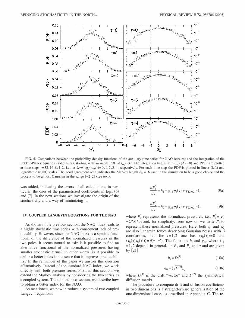
Figure 5 shows consecutive PDFs for ��=log2�tref / t�=0,1, 2, 3, and 4, corresponding to t=32, 16, 8, 4, and 2, respec-tively, starting from an initial PDF taken at tref =32. By inte-grating the Fokker-Planck equation, using the coefficients inEqs. �8�, one tests the validity of our approach, which as-sumes from the very beginning that the process is Markovianwithin a certain range of N increments, with a Markovlength �M =16. Notice that the noise level might be underes-timated since we did not consider the errors of the NAOindex measurements. Therefore, to improve the fits in Fig. 5we used a larger value for d1

�2�, keeping all the other coeffi-cients as given in �8�.

As one clearly sees from Fig. 5, the initial distributionretains its Gaussian shape through time and the PDFs of thedata �indicated by circles� are well fitted by the PDFs ob-tained from the integration of the Fokker-Planck equation�solid lines� within the range N�� �−2,2�. Thus, the Markovlength �M =16 chosen as well as the parametrization of theKramers-Moyal coefficients in Eqs. �6� and �7� seem to beappropriate for the present situation.

From the results in this section one concludes that thestandard NAO index N can be assumed as a stochastic pro-cess within the range �−2,2�, which corresponds approxi-mately to one standard deviation of the PDF of the originalN values plotted in Fig. 1. The fact that the Gaussian shapeis almost invariant for any time lag means that the time seriesis highly stochastic and that the forecast based on them isunreliable. This conclusion agrees with results of Colletteand Ausloos �13�. Here, however, a detailed error analysis

FIG. 4. The drift and diffusion coefficients,D�1� and D�2�, obtained from linear fits of the cor-responding conditional moments �see dashedlines in Fig. 3�. Here N� is given in the sameunits as the NAO index and varies within therange �−6,6� for tref =32 �top�, tref =64 �center�,and tref =96 �bottom�.

LIND et al. PHYSICAL REVIEW E 72, 056706 �2005�

056706-4

was added, indicating the errors of all calculations, in par-ticular, the ones of the parametrized coefficients in Eqs. �6�and �7�. In the next sections we investigate the origin of thestochasticity and a way of minimizing it.

IV. COUPLED LANGEVIN EQUATIONS FOR THE NAO

As shown in the previous section, the NAO index leads toa highly stochastic time series with consequent lack of pre-dictability. However, since the NAO index is a specific func-tional of the difference of the normalized pressures in thetwo poles, it seems natural to ask: Is it possible to find analternative functional of the normalized pressures havingsmaller stochastic terms? In other words, is it possible todefine a better index in the sense that it improves predictabil-ity? In the remainder of the paper we answer this questionaffirmatively. Instead of the standard NAO index, we workdirectly with both pressure series. First, in this section, weextend the Markov analysis by considering the two series asa coupled system. Then, in the next section, we describe howto obtain a better index for the NAO.

As mentioned, we now introduce a system of two coupledLangevin equations:

dP1*

d�= h1 + g11�1��� + g12�2��� , �9a�

dP2*

d�= h2 + g21�1��� + g22�2��� , �9b�

where Pi* represents the normalized pressures, i.e., Pi

*= �Pi

− �Pi�� /�i and, for simplicity, from now on we write Pi torepresent these normalized pressures. Here, both �1 and �2are also Langevin forces describing Gaussian noises with �correlations, i.e., for i=1,2 one has ��i����=0 and��i����i�����=���−���. The functions hi and gij, where i , j=1,2 depend, in general, on P1 and P2 and � and are givenby �21�

hi = Di�1�, �10a�

gij = �D�2��ij , �10b�

where D�1� is the drift “vector” and D�2� the symmetricaldiffusion matrix.

The procedure to compute drift and diffusion coefficientsin two dimensions is a straightforward generalization of theone-dimensional case, as described in Appendix C. The re-

FIG. 5. Comparison between the probability density functions of the auxiliary time series for NAO �circles� and the integration of theFokker-Planck equation �solid lines�, starting with an initial PDF at tref =32. The integration begins at t= tref ���=0� and PDFs are plottedat time steps t=32,16,8 ,4 ,2, i.e., at ��=log2�tref / t�=0,1 ,2 ,3 ,4, respectively. For each time step the PDF is plotted in linear �left� andlogarithmic �right� scales. The good agreement seen indicates the Markov length �M =16 used in the simulation to be a good choice and theprocess to be almost Gaussian in the range �−2,2� �see text�.

REDUCING STOCHASTICITY IN THE NORTH… PHYSICAL REVIEW E 72, 056706 �2005�

056706-5

sult of these computations are surfaces in the P1� P2 plane.As for the standard index, our simulations have shown thatthe dependence on � can be neglected here. Figure 6 showsthese surfaces for all the Kramers-Moyal coefficients with

the corresponding error bar at each grid point. At the bottomof each figure one sees the surfaces obtained from the data,while at the top the corresponding fitted surface is plotted.All fitted surfaces in Fig. 6 are quadratic forms

FIG. 6. �Color online� The Kramers-Moyal coefficients for the two coupled Langevin equations in �9�: �a� D1�1�, �b� D11

�2�, �c� D12�2�, �d� D2

�1�,�e� D21

�2�, and �f� D22�2�. Each plot shows a surface obtained from Eqs. �C1� in Appendix C and the corresponding fitted surface shifted for better

inspection.

LIND et al. PHYSICAL REVIEW E 72, 056706 �2005�

056706-6

S�P1,P2� = 1P1 + 2P12 + 3P2 + 4P2

2 + 5P1P2 + 6.

�11�

Table I gives the coefficients i for both the drift vector D�1�

and the diffusion matrix D�2� and also for the functions hi andgij defined in Eq. �10�.

From Table I one sees that the drift coefficients D1�1� and

D2�1� are approximately linear, i.e., apart from the indepen-

dent term, their dominant terms are P1 and P2, respectively.With this and from hi, Eq. �10a�, we can say that the deter-ministic parts of the Langevin equations �9� are almost un-coupled. In fact, the absence of coupling between the twodeterministic parts is not surprising since we are considering“instantaneous” coupling and, since both pressure sub-systems are distant from each other, any eventual influenceof one subsystem on the other should be characterized bysome delay time, large enough to enable propagation of in-formation.

As for the diffusion matrix, the two main diagonal ele-ments D11

�2� and D22�2� have significant contributions from the

quadratic terms. The same is true for the correspondingfunctions g11 and g22. Curiously, there is a fundamental dif-ference: while in g11 the quadratic term in P1

2 is much higherthan the one in P2

2, in function g22 both quadratic terms havesimilar contributions. Thus, one could argue that the normal-ized pressure P1 at the Azores high contributes more stronglyto the stochastic evolution of the pressure P2, than viceversa. In other words, there is a sort of unidirectional cou-pling of the stochastic forces between both subsystems, withP2 more strongly coupled to P1 than P1 to P2. This is analo-gous to recent results �24� indicating that P1 has a strongerinfluence than P2.

The off-diagonal terms D12�2�=D21

�2� and g12=g21, respec-tively, are dominated by P1P2 and, therefore, govern the

symmetrical part of the coupling between both subsystems.The symmetric part of the coupling is due to the symmetry ofthe diffusion matrix: D12

�2�=D21�2� �see Appendix C�.

Similar surfaces �not shown here� were obtained for hiand gij in Eq. �9�. The functions hi are identical to the driftcoefficient Di

�1� �Eq. �10a��. To determine functions gij onemust compute for each grid point a diffusion matrix andobtain its “square root” D�2� �Eq. �10b��. The matrix D�2�

is obtained from D�2� by imposing an orthogonal transforma-tion which diagonalizes D�2�, taking the positive square rootof the eigenvalues along the main diagonal and applying theinverse of the orthogonal transformation �21�. Note that forany pair �P1 , P2� the diffusion matrix is positive definite and,therefore, its eigenvalues are always positive, the corre-sponding square roots being real. Moreover, the same sym-metry of the diffusion matrix yields gij =gji.

From the results in this section one sees that, as for theanalysis based on a single Langevin equation, coupledLangevin equations still have high stochastic terms, in thesense that they contribute significantly to the evolution of thepressure variables. In the next section we show how to re-duce this stochasticity to a minimum.

V. REDUCING STOCHASTICITY VARIATIONALLY

The purpose of this section is to introduce a general varia-tional procedure allowing one to extract an optimal functionof the two pressure variables yielding a Langevin equationwith minimum stochasticity. As far as we know, this ap-proach to reduce stochasticity is original. It can be applied tospatially extended �coupled� systems characterized by sev-eral time series correlated �coupled� with each other.

We start by considering the two coupled Langevin equa-tions �9� whose coefficients hi and gij are given in Table I.

TABLE I. Parametrization coefficients of the drift vector D�1�, diffusion matrix D�2�, and of the functionsgij. Due to symmetry D21

�2�=D12�2� and g21=g12. From Eq. �10� one also has hi=Di

�1�.

1 2 3 4 5 6

D1�1� −0.920 0.085 −0.007 0.036 0.026 0.220

±0.062 ±0.096 ±0.058 ±0.093 ±0.089 ±0.073

D2�1� 0.000 −0.048 −1.093 0.040 0.032 0.342

±0.058 ±0.092 ±0.063 ±0.099 ±0.090 ±0.072

D11�2� −0.337 0.321 −0.089 −0.083 −0.280 0.818

±0.054 ±0.082 ±0.047 ±0.070 ±0.074 ±0.057

D22�2� −0.028 −0.209 −0.323 0.425 −0.186 0.870

±0.046 ±0.073 ±0.057 ±0.087 ±0.074 ±0.059

D12�2� −0.031 0.067 −0.091 −0.006 0.376 −0.184

±0.034 ±0.054 ±0.037 ±0.058 ±0.053 ±0.041

g11 −0.171 0.143 −0.065 −0.063 −0.147 0.906

±0.009 ±0.014 ±0.009 ±0.015 ±0.013 ±0.012

g22 −0.021 −0.119 −0.161 0.193 −0.089 0.931

±0.009 ±0.014 ±0.009 ±0.015 ±0.013 ±0.012

g12 −0.014 0.047 −0.046 0.009 0.181 −0.106

±0.009 ±0.014 ±0.009 ±0.015 ±0.013 ±0.012

REDUCING STOCHASTICITY IN THE NORTH… PHYSICAL REVIEW E 72, 056706 �2005�

056706-7

From Eqs. �9�, one can make a general transformation ofvariables �P1 , P2�→ �N1 ,N2� leading to a new system ofequations

dN1

d�= h1� + g11� �1��� + g12� �2��� , �12a�

dN2

d�= h2� + g21� �1��� + g22� �2��� , �12b�

where the new coefficients are

hi� = h1�Ni

�P1+ h2

�Ni

�P2, �13a�

gij� = g1j�Ni

�P1+ g2j

�Ni

�P2, �13b�

for i , j=1,2 and where the dependence on � is neglected,since this is what happens for our time series, as shown inthe previous section. One possible transformation of vari-ables would be N1= P1− P2 and N2= P1+ P2, which yields N1as the standard NAO index with strong stochasticity. Since,in general, the Jacobian of �13� does not vanish, many otherchoices are possible and the question we address now is forwhich choice are the stochastic terms minimal? To this end,we require that for one of the equations in �12�, say Eq.�12a�, both stochastic terms be as small as possible whencompared to the deterministic one. In other words, the de-pendence of N1 on P1 and P2 is such that a functional isminimized. We assume this functional to be

F =�g11� �L2

2 + �g12� �L2

2

�h1��L2

2 , �14�

where �f�P1 , P2��L2is the L2-norm of f�P1 , P2�:

�f�P1,P2��L2= �� �

f�P1,P2� 2dP1dP2�1/2

. �15�

As will be seen below, in practice, it is only necessary to takea finite interval for the integration in both variables, typically= �−1,1�� �−1,1�.

Without any additional condition it is difficult to minimizeF in Eq. �14� since it is a quotient of integrals. Therefore weimpose the additional constraint

� �

h1� 2

adP1dP2 = 1, �16�

where a is a suitable constant to be chosen in the next para-graph. Note that, since the constraint in Eq. �16� only im-poses a value for the deterministic part of the evolution andthe proposed variational method deals with the problem ofminimizing stochastic terms when compared with determin-istic ones, there are no spurious implications related with thiscondition.

The above considerations lead to a variational problem intwo variables where one seeks to minimize F under the con-straint �16�. This produces the Lagrangian

L = �g11� �2 + �g12� �2 + �� �h1��2

a− 1� , �17�

where � is the Lagrangian multiplier. Since we are still freeto chose a, without loss of generality we fix a=�. Thischoice is equivalent to writing the functions h1�, g11� , and g12�in Eq. �12a� in units of the L2 norm of the deterministicfunction h1�.

Substituting Eqs. �13� into Eq. �17�, inserting the La-grangian into the Euler-Lagrange equation

�L

�t−

�

�P1� �L

�� �N1

�P1�� −

�

�P2� �L

�� �N1

�P2�� = 0, �18�

and with elementary manipulation we arrive to the equation

A�N1

�P1

+ B�N1

�P2

+ C�2N1

�P12 + D�2N1

�P22 + E �2N1

�P1�P2

= F , �19�

where

A =�

�P1�g11

2 + g122 + h1

2� +�

�P2�g11g21 + g12g22 + h1h2� ,

�20a�

B =�

�P2�g21

2 + g222 + h2

2� +�

�P1�g11g21 + g12g22 + h1h2�

�20b�

C = g112 + g12

2 + h12, �20c�

D = g212 + g22

2 + h22, �20d�

E = 2�g11g21 + g12g22 + h1h2� , �20e�

F = − � �h1

�P1+

�h2

�P2� . �20f�

From the coefficients hi and gij in Table I one sees that allcoefficients in �20� are polynomials. More precisely, A andB are cubics, C, D, and E are quartics while F is a linearpolynomial.

In the range considered, the discriminant �E /2�2−CD isalways negative, indicating that Eq. �19� is an elliptic equa-tion �25�. Substituting the standard index N1= P1− P2 in Eq.�19� yields A−B=F, a condition not holding for most valuesof P1 and P2, as is illustrated in Fig. 7. This fact demon-strates an important fact, namely, that the standard NAO in-dex does not minimize the functional in Eq. �14� and, there-fore, is not the function of P1 and P2 with minimalstochasticity.

Discretizing Eq. �19� suitably one obtains N1 as a functionof the previous variables P1 and P2, satisfying the variationalproblem in Eq. �14�. In other words, one obtains a new func-tional N1�N1�P1 , P2� such that its corresponding Langevinequation, Eq. �12a�, has minimal stochasticity, as desired.Therefore, the new functional N1 is a better NAO index in

LIND et al. PHYSICAL REVIEW E 72, 056706 �2005�

056706-8

the sense that it enables more accurate forecasting, i.e., withless stochasticity, of the NAO system, extracted directly fromthe two measured pressure series. Similarly to the standardNAO index, forecasting of the pressure time series is stilldifficult and out from the scope of the present method. How-ever, from the new index one can extract relevant physicalinformation concerning the NAO system, for instance, anasymmetry in the coupling between both pressure sub-systems, as we explain next.

To integrate Eq. �19� we suppose that at the boundaries N1is a linear function of either P1 or P2, while at the corners of� one assumes N1=0 at �P1 , P2�= �−1,−1� and �P1 , P2�= �1,1�, N1=1 at �P1 , P2�= �1,−1� and N1=−1 at �P1 , P2�= �−1,1�. This choice of boundary conditions is motivated byclimatological facts concerning the NAO system. Namely, asmentioned in the Introduction, when P1 is large and P2 issmall, the NAO system is in the positive phase, correspond-ing to high values of the index. Inversely, when P1 is smalland P2 is large the index should be small. Thus, we assumethat the index N1 is maximal when P1 is maximal and P2 isminimal, and it is minimal when the opposite occurs.

Using centered differences to discretize derivatives in Eq.�19� and applying a successive over-relaxation algorithm�23� starting from the boundary conditions given in the lastparagraph, one obtains the optimal N1 as a function of P1 andP2. Figure 8 shows the surface N1�P1 , P2� obtained in thisway, where one clearly sees a deviation from a plane, mean-ing that N1 is not linear in P1 and P2 as the standard indexpresupposes. The best least-square fit for this surface is alsoa quadratic form

N1�P1,P2� = �1P1 + �2P12 + �3P2 + �4P2

2 + �5P1P2 + �6.

�21�

with

�1 = 0.5407 ± 0.0071, �22a�

FIG. 7. Function L=A−B−F �see Eqs. �20�� as a function of P1

and P2 in the range �−1,1�� �−1,1�. The contour line indicates L=0 for which Eq. �19� holds. Anywhere else the differential equa-tion is not satisfied, meaning that the standard NAO index is not theone with minimal stochasticity �see text�.

FIG. 8. Solution N1�P1 , P2� of Eq. �19� with linear boundaryconditions �see text�, minimizing the variational in Eq. �14�. In �a�and �b� the surface is shown in two different views, to emphasize itscurvature, showing that N1 is not linear in P1 and P2 as the standardNAO index. In �c� one sees the surface projected in the �P1 , P2�plane with contour lines, emphasizing the asymmetry around thesecondary diagonal P1=−P2.

REDUCING STOCHASTICITY IN THE NORTH… PHYSICAL REVIEW E 72, 056706 �2005�

056706-9

�2 = 0.2465 ± 0.0122, �22b�

�3 = − 0.6344 ± 0.0006, �22c�

�4 = 0.3370 ± 0.0011, �22d�

�5 = − 0.0170 ± 0.0122, �22e�

�6 = − 0.3384 ± 0.0005. �22f�

While Figs. 8�a� and 8�b� emphasize the curvature of thesurface N1�P1 , P2�, Fig. 8�c� shows the contour lines of thesurface projected in the �P1 , P2� plane. From this contourlines one clearly sees that there is an asymmetry due to thedifferent coefficients of the terms in P1 and P2.

While the new index defined above has a time serieswhich looks like that in Fig. 1 and has a correlation lengthslightly larger than the standard index, the diffusion coeffi-cient decreases significantly. In fact, as illustrated in Fig. 9,while the deterministic part remains almost the same �seeFig. 9�a�� the stochastic term controlled by the diffusion co-efficient decreases to approximately one-third of the coeffi-cient for the standard index. More precisely, repeating thesame Markov analysis as in Sec. III this time for the newindex, one obtains a fit for the drift and diffusion coefficientsof the form of Eqs. �6� and �7�, respectively, with the param-etrization

d1�1�,new = 0.120 ± 0.010, �23a�

d2�1�,new = − 1.074 ± 0.006, �23b�

d1�2�,new = 1.22 ± 0.02, �23c�

d2�2�,new = − 0.10 ± 0.01, �23d�

d3�2�,new = 0.414 ± 0.003. �23e�

By comparing Eqs. �23� with the previous Eqs. �8�, one seesthat, while the parametrization for the drift coefficient �deter-ministic term� remains approximately the same, the diffusion

coefficient ruling the stochasticity of the dynamics is nowmuch smaller. In particular, d1

�2�,new�d1�2� /3.

VI. DISCUSSION AND CONCLUSIONS

In this paper we performed a detailed Markov analysis ofthe standard monthly NAO index comparing it with a moregeneral analysis where, instead of the index derived from thepressure time series, we work with the measured pressuresdirectly. In both situations we find stochastic terms to belarge implying unreliable forecasting.

In order to reduce stochasticity we propose a generalvariational procedure which transforms variables from thetwo pressure time series into a pair of new variables, one ofthem having the minimum stochasticity possible. This varia-tionally optimized Markov analysis is general and may beapplied also to other systems characterized by two or moretime series, correlated �coupled� with each other, for in-stance, in spatially extended systems. We believe that thevariationally optimized Markov analysis represents a newdevelopment in the field. It should be helpful to deal withproblems where the familiar Markov analysis of single timeseries has already proved to be efficient.

To delimit the validity of the variationally optimized Mar-kov analysis one could check deterministic models, e.g., Lo-renz system, introducing noise as an additional term, and tryto obtain the optimal variable transformation from time se-ries extracted from the system. This test will be reportedelsewhere.

Concerning the particular case of the NAO system, al-though time series are relatively small �2135 points�, yield-ing large errors, the results above gave evidence that theNAO index may be interpreted as a Markovian process and,with the variational problem proposed above, it was possibleto obtain a functional relationship between both pressureshaving less stochasticity than the standard index. To use thisnew index for climatological purposes it would be necessaryto redefine the two different phases of the NAO, in order tounderstand the physical meaning of it.

The correlation length of the present time series is small,due to the large time lag �one month� between consecutive

FIG. 9. Kramers-Moyal coefficients, as afunction of the NAO index, for the optimized in-dex �diamonds� compared with the standard in-dex �circles�: �a� Drift coefficient D�1� and �b� dif-fusion coefficient D�2�. Here, the reference is tref

=32.

LIND et al. PHYSICAL REVIEW E 72, 056706 �2005�

056706-10

values of the time series. One possible way to furtherstrengthen the role of the deterministic part in the NAO sys-tem is to consider shorter time lags. Although climatologistsusually compute the standard NAO index between time in-tervals of one month or one year �8�, since the last 50 years,the daily pressure of the two NAO subsystems was also re-corded, enabling a standard definition of daily index similarto Eq. �1�, with a much larger correlation length and a largernumber of points. Preliminary results concerning the varia-tional Markov analysis of this daily measures indicate thatalso in that case an optimized functional relationship is ob-tained, with less stochasticity than the standard daily NAOindex. Moreover, by using time lags of one day instead ofone month or one year, one could ascertain which time lagbetween, say one day and one month, gives better results forforecasting. From the Markov analysis it is also possible toascertain which kind of noise, additive or multiplicative, thesystem has �26�. Finally, this approach could be extended byconsidering the impact of a delayed coupling, since the twosubsystems composing the NAO system force one anotherwithin a certain time scale. The study of these questions andtheir relevance for climatological purposes are now beingcarried out and will be presented elsewhere �27�.

ACKNOWLEDGMENTS

The authors thank Rudolf Friedrich, Joachim Peinke, andRudolf Hilfer for useful remarks and discussions. P.G.L.thanks Fundação para a Ciência e a Tecnologia �FCT�, Por-tugal, for financial support. J.A.C.G. thanks the Sonderfors-chungsbereich 404 of the DFG, Germany, and CNPq, Brazilfor financial support.

APPENDIX A: ERROR ANALYSIS

The error bars in Figs. 3 are obtained from standard erroranalysis, namely the error, function for the conditional mo-ments M�k� with k=1,2 read

�M�k��N�,�,��� =1

���

N�+��

���N��n��k�p , �A1�

where ��N��n�=N�+���n�−N��n� and �p is the error of theconditional probability, namely

�p =�pjoint

p�N�,��+

p�N�+��,� + ��;N�,���pref

�p�N�,���2 , �A2�

with �pjoint and �pref representing, respectively, the errors ofthe joint PDF p�N�+�� ,�+�� ;N� ,�� and of the PDF p�N� ,��of the reference time. These two errors are extracted directlyfrom the simulation as the square root of the number of val-ues inside each corresponding bin.

The error function for the drift and diffusion coefficientsin Fig. 4 are obtained directly from a linear regression of thecorresponding conditional moments as functions of ��,where the error function in Eq. �A1� for the conditional mo-ment is used as input. A similar error analysis was used forthe coefficients in the two-dimensional case �Fig. 6�.

The parametrizations in Eqs. �6� and �7�, in Table I and inEqs. �22� were performed using standard least-square proce-dures �23�.

APPENDIX B: INTEGRATING THE FOKKER-PLANCKEQUATION

We introduce the parametrizations �6� and �7� into theFokker-Planck equation

�

��p�N�,� N��,��� = LFPp�N�,� N��,��� , �B1�

where LFP is the operator

LFP = �−�

�N�

D�1��N�,�� +�2

�N�2D�2��N�,��� . �B2�

The initial condition p�N0 ,�0� is taken at t0= tref =32 andthe integration is carried out by means of a suitable discreti-zation scheme �21� yielding

p�N�+��,� + �� N�,��

=1

2 D�2��N�,����

�exp�−�N�+�� − N� − D�1��N�,�����2

4D�2��N�,����� . �B3�

The Fokker-Planck Eq. �B1� describes the evolution ofconditional PDFs. To know at each time � the single PDFp�N�+�� ,�+���, as the ones shown in Fig. 5 for time-steps��=1, 2, 3, 4 and 5, one must integrate at each time step theconditional PDF multiplied by the previous single PDF. Thisis done by using the Chapman-Kolmogorov equation

p�N�+��,� + ��� =� p�N�+��,� + �� N�,��p�N�,��dN�.

�B4�

APPENDIX C: DRIFT AND DIFFUSION COEFFICIENTSIN TWO-DIMENSIONS

For the two-dimensional case of two coupled Langevinequations, Eqs. �9�, the Kramers-Moyal coefficients read �21�

Di�1��P1,P2,�� = lim

��→0Mi

�1��P1,P2,�,��� , �C1a�

Dij�2��P1,P2,�� = 1

2 lim��→0

Mij�2��P1,P2,�,��� , �C1b�

where i , j=1,2 and conditional moments are given by

Mi�1��P1,P2,�,��� �

1

���Pi�

�Pip , �C2a�

Mij�2��P1,P2,�,��� �

1

���

Pi�,Pj�

�Pi�Pjp , �C2b�

REDUCING STOCHASTICITY IN THE NORTH… PHYSICAL REVIEW E 72, 056706 �2005�

056706-11

where �Pi= Pi���+���− Pi��� and where now the sum isover the bins discretization, namely the PDF of Pi,j� ��+���,and p� p�P� ���+��� ,�+�� P� ��� ,�� is the conditional prob-

ability of observing the two values P� �= �P1� , P2�� at �+��

knowing that the values P� = �P1 , P2� were observed at �. Asone clearly sees from Eq. �C2b� the matrix of second orderconditional moments and consequently D�2� are symmetric,D12

�2�=D21�2�.

�1� P. D. Jones, T. J. Osborn, and K. R. Briffa, Science 292, 662�2001�.

�2� K. Higuchi, J. Huang, and A. Shabbar, Int. J. Climatol. 19,1119 �1999�.

�3� H. Paeth, M. Latif, and A. Hense, Clim. Dyn. 21, 63 �2003�.�4� C. Appenzeller, T. F. Stocker, and M. Anklin, Science 282,

446 �1998�.�5� C. Wunsch, Bull. Am. Meteorol. Soc. 80, 245 �1999�.�6� S. Jevrejeva, J. C. Moore, and A. Grinsted, J. Geophys. Res.

108, 4677 �2003�.�7� J. L. Melice and J. Servain, Clim. Dyn. 20, 447 �2003�.�8� H. Wanner, S. Bronnimann, C. Casty, D. Gyalistras, J. Luter-

bacher, C. Schmutz, D. B. Stephenson, and E. Xoplaki, Surv.Geophys. 22, 321 �2001�.

�9� J. Hurrel, Science 279, 676 �1995�.�10� O. A. Lucero and N. C. Rodriguez, Int. J. Climatol. 22, 805

�2002�.�11� Data are available at http://www.cru.uea.ac.uk/cru/data/

nao.htm.�12� D. B. Stephenson, V. Pavan, and R. Bojariu, Int. J. Climatol.

20, 1 �2000�.�13� C. Collette and M. Ausloos, Int. J. Mod. Phys. C 15, 1353

�2004�.�14� Ch. Renner, J. Peinke, and R. Friedrich, J. Fluid Mech. 433,

383 �2001�.

�15� J. Gradisek, S. Siegert, R. Friedrich, and I. Grabec, Phys. Rev.E 62, 3146 �2000�.

�16� R. Friedrich, J. Peinke, and Ch. Renner, Phys. Rev. Lett. 84,5224 �2000�.

�17� M. Waechter, F. Riess, Th. Schimmel, U. Wendt, and J. Peinke,Eur. Phys. J. B 41, 259 �2004�.

�18� K. Ivanova and M. Ausloos, J. Geophys. Res. 107, 4708�2002�.

�19� P. Sura, J. Atmos. Sci. 60, 654 �2003�.�20� R. Friedrich and J. Peinke, Phys. Rev. Lett. 78, 863 �1997�.�21� H. Risken, The Fokker Planck Equation �Springer, Berlin,

1984�.�22� H. D. I. Abarbanel, R. Brown, J. J. Sidorowich, and L. S.

Tsimring, Rev. Mod. Phys. 65, 1331 �1993�.�23� W. H. Press, B. P. Flannery, S. A. Teukolsky, and W. T. Vet-

terling, Numerical Recipes �Cambridge University Press, Cam-bridge, 1992�.

�24� T. Jónsson and M. Miles, Geophys. Res. Lett. 28, 4231 �2001�.�25� B. Epstein, Partial Differential Equations �McGraw-Hill, New

York, 1962�.�26� M. Siefert, A. Kittel, R. Friedrich, and J. Peinke, Europhys.

Lett. 61, 466 �2003�.�27� P. G. Lind, A. Mora, J. A. C. Gallas, and M. Haase �unpub-

lished�.

LIND et al. PHYSICAL REVIEW E 72, 056706 �2005�

056706-12