Refined error estimates for the Riccati equation with applications to the angular Teukolsky equation

arX

iv:1

307.

6470

v3 [

mat

h.C

A]

17

Feb

2015

REFINED ERROR ESTIMATES FOR THE RICCATI EQUATION

WITH APPLICATIONS TO THE ANGULAR TEUKOLSKY

EQUATION

FELIX FINSTER AND JOEL SMOLLER

JULY 2013

Abstract. We derive refined rigorous error estimates for approximate solutions ofSturm-Liouville and Riccati equations with real or complex potentials. The approxi-mate solutions include WKB approximations, Airy and parabolic cylinder functions,and certain Bessel functions. Our estimates are applied to solutions of the angularTeukolsky equation with a complex aspherical parameter in a rotating black holeKerr geometry.

Contents

1. Introduction 22. A Sturm-Liouville Operator with a Complex Potential 33. General Invariant Region Estimates for the Riccati Flow 43.1. An Invariant Disk Estimate 43.2. The T -Method 63.3. The κ-Method 93.4. Lower Bounds for Im y 104. Semiclassical Estimates for a General Potential 124.1. Estimates in the Case ReV < 0 124.2. Estimates in the Case ReV > 0 145. Semiclassical Estimates for the Angular Teukolsky Equation 185.1. Estimates in the Case ReV < 0 185.2. Estimates in the Case ReV > 0 196. Parabolic Cylinder Estimates 216.1. Estimates of Parabolic Cylinder Functions 216.2. Applications to the Angular Teukolsky Equation 257. Estimates for a Singular Potential 277.1. The case L = 0 277.2. The case L > 0 288. Estimates for the Angular Teukolsky Equation near the Poles 298.1. The Case L = 0 308.2. The Case L > 0 31References 33

J.S. is supported in part by the National Science Foundation, Grant No. DMS-1105189.

1

http://arxiv.org/abs/1307.6470v3

2 F. FINSTER AND J. SMOLLER

1. Introduction

The Teukolsky equation arises in the study of electromagnetic, gravitational andneutrino-field perturbations in the Kerr geometry describing a rotating black hole(see [2, 13]). In this equation, the spin of the wave enters as a parameter s ∈0, 12 , 1, 32 , 2, . . . (the case s = 0 reduces to the scalar wave equation). The Teukolskyequation can be separated into radial and angular parts, giving rise to a system ofcoupled ODEs. Here we shall analyze the angular equation, also referred to as thespin-weighted spheroidal wave equation. It can be written as the eigenvalue equation

AΨ = λΨ , (1.1)

where the spin-weighted spheroidal wave operator A is an elliptic operator with smoothcoefficients on the unit sphere S2. More specifically, choosing polar coordinates ϑ ∈(0, π) and ϕ ∈ [0, 2π), we have (see for example [14])

AΘ = λΘ with A = − ∂

∂ cos ϑsin2 ϑ

∂

∂ cosϑ+

1

sin2 ϑ

(

Ω sin2 ϑ+ i∂

∂ϕ− s cos ϑ

)2

.

Here Ω ∈ C is the aspherical parameter. In the special case Ω = 0, we obtain the spin-weighted Laplacian, whose eigenvalues and eigenfunctions can be given explicitly [11].In the case s = 0 and Ω 6= 0, one gets the spheroidal wave operator as studied in [10].Setting Ω = 0 and s = 0, one simply obtains the Laplacian on the sphere. Weare mainly interested in the cases s = 1 of an electromagnetic field and s = 2 of agravitational field.

As the spin-weighted spheroidal wave operator is axisymmetric, we can separate outthe ϕ-dependence with a plane wave ansatz,

Ψ(ϑ,ϕ) = e−ikϕ Θ(ϑ) with k ∈ Z .

Then A becomes the ordinary differential operator

A = − ∂

∂ cos ϑsin2 ϑ

∂

∂ cos ϑ+

1

sin2 ϑ

(

Ω sin2 ϑ+ k − s cos ϑ)2

. (1.2)

To analyze the eigenvalue equation (1.1), we consider this operator on the Hilbertspace H = L2((−1, 1), d cos ϑ) with domain of definition D(A) = C∞

0 ((−1, 1)). In thisformulation, the spheroidal wave equation also applies in the case of half-integer spin(to describe neutrino or Rarita-Schwinger fields), if k is chosen to be a half-integer.Thus in what follows, we fix the parameters s and k such that

2s ∈ N0 and k − s ∈ Z .

In most applications, the aspherical parameter Ω is real. However, having contourmethods for the Teukolsky equation in mind (similar as worked out in [4] for thescalar wave equation), we must consider the case that Ω is complex. This leads to themajor difficulty that the potential in (1.2) also becomes complex, so that the angularTeukolsky operator is no longer a symmetric operator. At least, it suffices to considerthe case when |Ω| is large, whereas the imaginary part of Ω is uniformly bounded, i.e.

|Ω| > C and | ImΩ| < c (1.3)

for suitable constants C and c. We are aiming at deriving a spectral representation forthis non-symmetric angular Teukolsky operator, which will involve complex eigenvaluesand possibly Jordan chains. In order to derive this spectral representation, we musthave detailed knowledge of the solutions of the Sturm-Liouville equation (1.1). Our

REFINED ERROR ESTIMATES FOR THE RICCATI EQUATION 3

strategy for getting this detailed information is to first construct approximate solutionsby “glueing together” suitable WKB, Airy, Bessel and parabolic cylinder functions,and then to derive rigorous error estimates. The required properties of the specialfunctions were worked out in [9]. Our error estimates are based on the invariant regiontechniques in [8]. These techniques need to be refined considerably in order to beapplicable to the angular Teukolsky equation. Since these refined error estimates canbe applied in a much more general context, we organize this paper by first developingthe general methods and then applying them to the angular Teukolsky equation.

This paper is part of our program which aims at proving linear stability of the Kerrblack hole under perturbations of general spin (for another approach towards this goalwe refer to [1]). The estimates derived in the present paper play an important rolein this program. Indeed, they are a preparation for proving a spectral resolution forthe angular Teukolsky equation involving projectors onto finite-dimensional invariantsubspaces [6] (related results on the angular operator for scalar waves can be foundin [5, 3]). The next step will be to derive an integral representation for the timeevolution operator of the full Teukolsky equation in the same spirit as carried out inthe Schwarzschild geometry in [7].

The paper is organized as follows. We begin the analysis by transforming the an-gular Teukolsky equation into Sturm-Liouville form with a complex potential (Sec-tion 2). We then develop invariant region estimates for a general potential (Section 3).We proceed by deriving WKB estimates (Section 4), and then applying them to theangular Teukolsky equation (Section 5). In Section 6 we derive error estimates forparabolic cylinder approximations. These include estimates for Airy approximationsas a special case. Section 7 is devoted to the properties of Bessel function solutionsof Sturm-Liouville equations with singular potentials. Finally, in Section 8 we usethese properties to analyze solutions of the angular Teukolsky equation near the polesat ϑ = 0 and π.

2. A Sturm-Liouville Operator with a Complex Potential

In order to bring the operator (1.2) to the standard Sturm-Liouville form, we firstwrite the operator in the variable u = ϑ ∈ (0, π),

A = − 1

sinu

d

dusinu

d

du+

1

sin2 u

(

Ω sin2 u+ k − s cos u)2

.

Introducing the function Y by

Y =√sinuΘ , (2.1)

we get the eigenvalue equation

B φ = λ φ ,

where

B = − 1√sinu

d

dusinu

d

du

1√sinu

+1

sin2 u(Ω sin2 u+ k − s cosu)2

= − d2

du2+

1

2

cos2 u

sin2 u−

√sinu

(

1√sinu

)′′+

1

sin2 u(Ω sin2 u+ k − s cosu)2

= − d2

du2− 1

4

cos2 u

sin2 u− 1

2+

1

sin2 u(Ω sin2 u+ k − s cos u)2 .


Thus φ satisfies the Sturm-Liouville equation(

− d2

du2+ V

)

φ = 0 (2.2)

with the potential V given by

V = Ω2 sin2 u+

(

k2 + s2 − 1

4

)

1

sin2 u− 2sΩcos u− 2sk

cos u

sin2 u− µ (2.3)

and µ is the constant

µ = λ− 2Ωk + s2 +1

4.

The transformation (2.1) from Θ to Y becomes a unitary transformation if the in-tegration measure in the corresponding Hilbert spaces is transformed from sinu duto du. Thus the eigenvalue problem (1.1) on H is equivalent to (2.2) on the Hilbertspace L2((0, π), du).

3. General Invariant Region Estimates for the Riccati Flow

3.1. An Invariant Disk Estimate. Our method for getting estimates for solutionsof the Sturm-Liouville equation (2.2) is to use invariant region estimates for the corre-sponding Riccati equation. We here outline and improve the methods introduced in [8].Clearly, the solution space of the linear second order equation (2.2) is two-dimensional.For two solutions φ1 and φ2, the Wronskian w(φ1, φ2) defined by

w(φ1, φ2) = φ1φ′2 − φ′

1φ2

is a constant. Integrating this equation, we can express one solution in terms of theother, e.g.

φ2(u) = φ1(u)

(∫ u w

φ21

+ const

)

.

Thus from one solution one gets the general solution by integration and taking linearcombinations. With this in mind, it suffices to get estimates for a particular solution φof the Sturm-Liouville equation, which we can choose at our convenience.

Setting

y =φ′

φ,

the function y satisfies the Riccati equation

y′ = V − y2 . (3.1)

Considering u as a time variable, the Riccati equation can be regarded as describinga flow in the complex plane, the so-called Riccati flow. In order to estimate y, wewant to find an approximate solution m(u) together with a radius R(u) such that nosolution y of the Riccati equation may leave the circles with radius R centered at m.More precisely, we want that the implication

∣

∣y(u0)−m(u0)∣

∣ ≤ R(u0) =⇒∣

∣y(u1)−m(u1)∣

∣ ≤ R(u1)

holds for all u1 > u0 and u0, u1 ∈ I. We say that these circles are invariant under theRiccati flow. Decomposing m into real and imaginary parts,

m(u) = α(u) + iβ(u) , (3.2)


our strategy is to prescribe the real part α, whereas the imaginary part β will bedetermined from our estimates. Then the functions U and σ defined by

U = ReV − α2 − α′ (3.3)

σ(u) = exp

(∫ u

2α

)

, (3.4)

which depend only on the known functions V and α, can be considered as givenfunctions. Moreover, we introduce the so-called determinator D by

D = 2αU +U ′

2+ β ImV . (3.5)

In our setting of a complex potential, the determinator involves β and will thus beknown only after computing the circles. The following Theorem is a special case of [8,Theorem 3.3] (obtained by choosing W ≡ U).

Theorem 3.1 (Invariant disk estimate). Assume that for a given function α ∈C1(I) one of the following conditions holds:

(A) Defining real functions R and β on I by

(R − β)(u) = − 1

σ

∫ u

σ ImV (3.6)

(R + β)(u) =U(u)

(R− β)(u), (3.7)

assume that the function R− β has no zeros, R ≥ 0, and

(R− β)D ≥ 0 . (3.8)

(B) Defining real functions R and β on I by

(R+ β)(u) =1

σ

∫ u

σ ImV (3.9)

(R− β)(u) =U(u)

(R+ β)(u), (3.10)

assume that the function R+ β has no zeros, R ≥ 0, and

(R+ β)D ≥ 0 . (3.11)

Then the circle centered at m(u) = α + iβ with radius R(u) is invariant on I underthe Riccati flow (3.1).

If this theorem applies and if the initial conditions y(u0) lie inside the invariantcircles, we have obtained an approximate solution m, (3.2), together with the rigorouserror bound

∣

∣y(u)−m(u)∣

∣ ≤ R(u) for all u ≥ u0 .

In order to apply the above theorems, we need to prescribe the function α. Whenusing Theorem 3.1, the freedom in choosing α must be used to suitably adjust the signof the determinator. One method for constructing α is to modify the potential V to anew potential V for which the Sturm-Liouville equation has an explicit solution φ,

(

− d2

du2+ V

)

φ = 0 . (3.12)


We let y := φ′/φ be the corresponding Riccati solution,

y′ = V − y2 , (3.13)

and define α as the real part of y. Denoting the imaginary part of y by β, we thushave

y = α+ iβ . (3.14)

Writing the real and imaginary parts of the Riccati equation in (3.14) separately, weobtain

α′ = Re V − α2 + β2 , β′ = Im V − 2αβ . (3.15)

In this situation, the determinator and the invariant disk estimates can be written in aparticularly convenient form, as we now explain. First, integrating the real part of y,we find that the function σ, (3.4), can be chosen as

σ(u) = exp(

∫ u

2α)

= exp(

2Re

∫ u φ′

φ

)

= |φ|2 . (3.16)

Moreover, applying the first equation in (3.15) to (3.3), we get

U = Re(V − V )− β2 . (3.17)

Differentiating (3.17) and using the second equation in (3.15), we obtain

U ′ = Re(V − V )′ + 4αβ2 − 2β Im V .

Substituting this equation together with (3.17) into (3.5) gives (cf. [8, Lemma 3.4])

D = 2αRe(V − V ) +1

2Re(V − V )′ − β Im V + β ImV . (3.18)

3.2. The T -Method. The main difficulty in applying Theorem 3.1 is that one mustsatisfy the inequalities (3.8) or (3.11) by giving the determinator a specific sign. Inthe case |β| > R, we know that Theorem 3.1 applies no matter what the sign ofthe determinator is, because either (3.8) or (3.11) is satisfied. This suggests that bysuitably combining the cases (A) and (B), one should obtain an estimate which doesnot involve the sign of D. The next theorem achieves this goal. It is motivated by themethod developed in [5, Lemma 4.1] in the case of real potentials. The method worksonly under the assumption that the function U given by (3.3) or (3.17) is negative.

Theorem 3.2. Assume that U < 0. We define β and R by

β =

√

|U |2

(

T +1

T

)

, R =

√

|U |2

(

T − 1

T

)

(3.19)

where T ≥ 1 is a real-valued function which satisfies the differential inequality

T ′

T≥∣

∣

∣

∣

D

U

∣

∣

∣

∣

− ImV√

|U |T 2 − 1

2T. (3.20)

Then the circle centered at m(u) = α(u) + iβ(u) with radius R(u) is invariant underthe Riccati flow (3.1).


Proof. Making the ansatz (3.19) with a free function T ≥ 1, the equations (3.7)and (3.10) hold automatically. Moreover, we see that 0 ≤ R < β, so that if D ≤ 0 wecan apply case (A), whereas if D > 0 we are in case (B). From (3.5) and (3.4), wefind that

D

U= 2α+

U ′

2U− ImV

|U | β =(σ√

|U |)′

σ√

|U |− ImV

2√

|U |

(

T +1

T

)

. (3.21)

In case (A), differentiating (3.6) gives the equation(

−σ√

|U |T

)′

= −σ Im√V .

Solving for T ′/T gives

T ′

T=

(σ√

|U |)′

σ√

|U |− ImV√

|U |T .

Substituting (3.21) and using (3.19), we obtain

T ′

T=

D

U− ImV

|U | R . (3.22)

In case (B), we obtain similarly(

σ√

|U | T)′

= σ Im√V

and thus

T ′

T= −(σ

√

|U |)′

σ√

|U |+

ImV√

|U |1

T.

Again using (3.21) and (3.19), we obtain

T ′

T= −D

U− ImV

|U | R . (3.23)

Using that the quotient D/U is positive in case (A) and negative in case (B), we cancombine (3.22) and (3.23) to the differential equation

T ′

T=

∣

∣

∣

∣

D

U

∣

∣

∣

∣

− ImV

|U | R ,

which now holds independent of the sign of the determinator. Using (3.19), thisequation can be written as

T ′

T=

∣

∣

∣

∣

D

U

∣

∣

∣

∣

− ImV√

|U |T 2 − 1

2T.

If T solves this equation, then we know from Theorem 3.1 that we have invariantcircles for the Riccati flow. Replacing the equality by an inequality, the function Tgrows faster. Since increasing T increases the circle defined by (3.19), we again obtaininvariant regions.

The next theorem gives a convenient method for constructing a solution of theinequality (3.20).


Theorem 3.3. Assume that U < 0. We choose a real-valued function g and definethe function T by

log T (u) =

∫ u

E ,

where

E =∣

∣E1 + E2 + E3

∣

∣+ E4

and

E1 :=1

2 |U |(

4αRe(V − V ) + Re(V − V )′)

E2 :=β

|U | Im(V − V )

E3 := − ImV

|U |Re(V − V )√

|U |+ β

E4 :=| ImV |√

|U |g(u) .

Then the circle centered at m(u) = α(u) + iβ(u) with radius R(u) is invariant underthe Riccati flow (3.1), provided that the following condition holds:

g ≥ −T − 1

Tif ImV ≥ 0

g ≥ T − 1 if ImV < 0 .

(3.24)

Proof. According to the first equation in (3.19),

∣

∣

∣β −

√

|U |∣

∣

∣=√

|U | (T − 1)2

2T.

Using this equation in (3.18), we obtain

|D| ≤∣

∣

∣2αRe(V − V ) +

1

2Re(V − V )′

+ β Im(V − V ) +(

√

|U | − β)

ImV∣

∣

∣+√

|U | | ImV | (T − 1)2

2T.

Applying the identities

√

|U | − β =|U |2 − β2

√

|U |+ β= −Re(V − V )

√

|U |+ β

(where in the last step we applied (3.17) and used that U < 0), the right side of (3.20)can be estimated by

∣

∣

∣

∣

D

U

∣

∣

∣

∣

− ImV√

|U |T 2 − 1

2T≤ |E1 + E2 + E3|+

| ImV |√

|U |(T − 1)2

2T− ImV√

|U |T 2 − 1

2T.

Simplifying the last two summands in the two cases ImV ≥ 0 and ImV < 0 gives theresult.


3.3. The κ-Method. We now explain an alternative method for getting invariantregion estimates. This method is designed for the case when |β| < R. In this case, thefactors R∓ β in (3.8) and (3.11) have the same sign. Therefore, Theorem 3.1 appliesonly if the determinator has has the right sign. In order to arrange the correct signof the determinator, we must work with driving functions (for details see Section 4.2).When doing this, we know a-priori whether we want to apply Theorem 3.1 in case (A)or (B). With this in mind, we may now restrict attention to a fixed case (A) or (B). Inorder to treat both cases at once, whenever we use the symbols ± or ∓, the upper andlower signs refer to the cases (A) and (B), respectively. Differentiating (3.6) and (3.9)and using the form of σ, (3.4), we obtain

(R ∓ β)′ = −2α (R ∓ β)∓ ImV .

Combining this differential equation with the second equation in (3.15), we get(

β ∓R− β)′= Im(V − V )− 2α

(

β ∓R− β)

.

This differential equation can be integrated. Again using (3.4), we obtain

β ∓R− β = κ with (3.25)

κ :=1

σ

(∫ u

σ Im(V − V ) + C

)

, (3.26)

where the integration constant C must be chosen such that (3.25) holds initially.Solving (3.25) for β and using the resulting equation in (3.18) gives

D = 2α Re(V − V ) +1

2Re(V − V )′ + β Im(V − V ) + (κ±R) ImV . (3.27)

The combination κ±R in (3.27) has the following useful representation.

Lemma 3.4. The function κ±R is given by

κ±R =κ2 − Re(V − V )

2 (β + κ). (3.28)

Proof. According to (3.25) and (3.7), (3.10),

R∓ β = ∓(β + κ) , R± β =U

R∓ β= ∓ U

β + κ

and thus

R = ∓1

2

(

(β + κ) +U

β + κ

)

= ∓U + (β + κ)2

2 (β + κ).

It follows that

κ±R = κ− U + (β + κ)2

2 (β + κ)=

2κβ + 2κ2 − U − (β + κ)2

2 (β + κ)=

κ2 − U − β2

2 (β + κ),

and using (3.17) gives the result.

The above relations give the following method for getting invariant region estimates.First, we choose an approximate potential V having an explicit solution y = α + iβ.Next, we compute σ by (3.4) or (3.16) and compute the integral (3.26) to obtain κ.The identity (3.28) gives the quantity κ ± R. Substituting this result into (3.27), weget an explicit formula for the determinator. Instead of explicit computations, one canclearly work with inequalities to obtain estimates of the determinator. The key point


is to use the freedom in choosing V to give the determinator a definite sign. Once thishas been accomplished, we can apply Theorem 3.1 in cases (A) or (B).

The method so far has the disadvantage that the function β+κ in the denominatorin (3.28) may become small, in which case the summand (κ±R) ImV in the determi-nator (3.27) gets out of control. Our method for avoiding this problem is to increase κin such a way that the solution stays inside the resulting disk. This method only worksin case (B) of Theorem 3.1.

Proposition 3.5. Assume that y is a solution of the Riccati equation (3.1) in the upperhalf plane Im y > 0. Moreover, assume that D > 0. For an increasing function g weset

κ(u) =g(u)

σ(u)+

1

σ

∫ u

σ Im(V − V ) (3.29)

and choose R and β according to (3.25) and (3.10),

R+ β = β + κ , R− β =U

R+ β. (3.30)

Then the circle centered at m = α + iβ with radius R is invariant on I under theRiccati flow. Moreover, Lemma 3.4 remains valid.

Proof. According to Theorem 3.1 (B) and (3.25), the identities (3.30) give rise toinvariant disk estimates if we choose

β + κ = β +const

σ(u)+

1

σ

∫ u

σ Im(V − V ) . (3.31)

If the constant is increased, the upper point R + β of the circle moves up. In thecase β−R ≥ 0, the second equation in (3.30) implies that the lower point β−R of thecircle moves down. As a consequence, the disk increases if the constant is made larger.Likewise, in the case β − R < 0, the circle intersects the axis Im y = 0 in the twopoints α ±

√U , which do not change if the constant is increased. As a consequence,

the intersection of the disk with the upper half plane increases if the constant is madelarger. Thus in both cases, the solution y(u) stays inside the disk if the constant isincreased.

We next subdivide the interval I into subintervals. On each subinterval, we may usethe formula (3.31) with an increasing sequence of constants. Letting the number ofsubintervals tend to infinity, we conclude that we obtain an invariant region estimateif the constant in (3.31) is replaced by a monotone increasing function g(u).

3.4. Lower Bounds for Im y. We begin with an estimate in the case when ImV ispositive.

Lemma 3.6. Suppose that y is a solution of the Riccati equation (3.1) for a potentialwith the property

ImV > 0 . (3.32)

Assume furthermore that Im y(u0) > 0. Then

Im y(u) ≥ Im y(u0) exp

(

−2

∫ u

u0

Re y

)

. (3.33)

Moreover, the Riccati flow preserves the inequality

Im y(u) ≥ inf[u0,u]

ImV

2 Re y. (3.34)


Proof. Taking the imaginary part of (3.1) gives

Im y′ = ImV − 2Re y Im y . (3.35)

From (3.32), we obtain

log′ | Im y| ≥ −2Re y .

Integration gives (3.33). In particular, Im y stays positive.For the proof of (3.34) we assume conversely that this inequality holds at some u1 >

u0 but is violated for some u2 > u1. Thus, denoting the difference of the left and rightside of (3.34) by g, we know that g(u1) ≥ 0 and g(u2) < 0. By continuity, there isa largest number u ∈ [u1, u2) with g(u) = 0. According to the mean value theorem,there is v ∈ [u, u2] with g′(v) = g(u2)/(u2 − u) < 0. Since the function on the right ismonotone decreasing in u, this implies that Im y′(v) < 0. Using (3.35), we obtain at v

0 > Im y′(v) = ImV (v) − 2Re y(v) Im y(v) .

If Re y ≤ 0, the infimum in (3.34) is also negative, so that there is nothing to prove.In the remaining case Re y > 0, we can solve for Im y to obtain

Im y(v) >ImV (v)

2Re y(v)≥ inf

[u0,v]

ImV

2Re y.

Hence g(v) > 0, a contradiction.

The following estimate applies even in the case when ImV is negative. The methodis to combine a Gronwall estimate with a differential equation for Im y.

Lemma 3.7. Let y be a solution of the Riccati equation (3.1) on an interval [u−, u+]and

max[u

−,u+]

√

|V | (u+ − u−) ≤ c .

Assume that Im y(u−) ≥ 0. Then there is a constant C depending only on c such that

Im y(u) ≥ 1

CIm y(u−)−C (u− u−)

∣

∣

∣min[u

−,u]

ImV∣

∣

∣.

Proof. Let φ(u) = exp(∫ u

y) be the corresponding solution of the Sturm-Liouville

equation (2.2). Setting κ = max[u−,u+] |V | 12 , we write the Sturm-Liouville equation as

the first order system

Ψ′(u) =

(

0 κV/κ 0

)

Ψ(u) with Ψ(u) :=

(

κφ(u)φ′(u)

)

.

Using that∫ u+

u−

(

κ+|V |κ

)

du ≤ max[u

−,u+]

√

|V | (u+ − u−) ≤ c ,

a Gronwall estimate yields

1

c2‖Ψ(u−)‖ ≤ ‖Ψ(u)‖ ≤ c2 ‖Ψ(u−)‖ , (3.36)

where c2 depends only on c. This inequality bounds the combination κ2|φ|2 + |φ′|2from above and below. However, it does not rule out zeros of the function φ. To thisend, we differentiate the identity

Im(φφ′) = Im(|φ|2 y) = |φ|2 Im y


to obtain the differential equation

d

du

(

|φ|2 Im y)

= ImV |φ|2 .

Integrating this differential equation, we obtain

|φ|2 Im y∣

∣

∣

u= |φ|2 Im y

∣

∣

∣

u−

+

∫ u

u−

ImV |φ|2

and thus

|φ|2 Im y∣

∣

∣

u≥ |φ|2 Im y

∣

∣

∣

u−

+(

min[u

−,u+]

ImV)

max[u

−,u+]

|φ|2 (u+ − u−) .

Applying the Gronwall estimate (3.36) gives the result.

4. Semiclassical Estimates for a General Potential

4.1. Estimates in the Case ReV < 0. We now consider the Riccati equation (3.1)on an interval I. We assume that the region I is semi-classical in the sense that theinequalities

supI

|V ′| ≤ ε infI|V | 32 , sup

I

|V ′′| ≤ ε2 infI|V |2 , sup

I

|V ′′′| ≤ ε3 infI|V | 52 (4.1)

hold, with a positive constant ε ≪ 1 to be specified later.In this section, we derive estimates in the case ReV < 0. As the approximate

solution, we choose the usual WKB wave function

φ(u) = V − 1

4 exp(

∫ u

u0

√V)

.

It is a solution of the Sturm-Liouville equation (3.12) with

V := V +5

16

(V ′)2

V 2− 1

4

V ′′

V. (4.2)

The corresponding solution of the Riccati equation (3.13) becomes

y =φ′

φ=

√V − V ′

4V. (4.3)

Moreover, we can compute the function σ from (3.16),

σ(u) = |φ(u)|2 = |V |− 1

2 e2∫u

u0Re

√V.

We begin with an estimate in the case ImV ≥ 0.

Lemma 4.1. Assume that on the interval I := [u0, umax], the potential V satisfies the

inequalities (4.1) with

ε <1

8. (4.4)

Moreover, we assume that on I,

Im√V > Re

√V ≥ 0 . (4.5)

Then Theorem 3.3 applies with g ≡ 0 and

log T (u) ≤ 64 ε2 infI|V |2

∫ u 1

|V | 32. (4.6)


Proof. The inequalities (4.5) clearly imply that ImV ≥ 0. Moreover, a straightforwardcalculation using (3.17), (3.14), (4.3) and (4.2) shows that

|U + Im2√V | ≤ 1

2

|V ′|√

|V |+

3

8

|V ′|2|V |2 +

1

4

|V ′′||V | ≤ 3ε |V | ,

where in the last step we used (4.1) and (4.4). Combining this inequality with (4.5)and (4.4), we conclude that

U < −1

4|V | < 0 .

Hence Theorem 3.3 applies. Since ImV ≥ 0, we can satisfy the condition (3.24) bychoosing g ≡ 0.

A straightforward calculation and estimate (which we carried out with the help ofMathematica) yields

|E1 + E2| ≤ 40 ε2infI |V |2

|V | 32(4.7)

|E3| =| ImV ||U |

|Re(V − V )|√

|U |+ β≤ 24 ε2

infI |V |2

|V | 32, (4.8)

giving the result.

The integral in (4.6) can be estimated efficiently if we assume that |V | satisfies aweak version of concavity:

Lemma 4.2. Suppose that on the interval [u0, u], the potential V satisfies the inequal-ities

|V (τ)| ≥ τ − u0u− u0

|V (u)|+ u− τ

u− u0|V (u0)| . (4.9)

Then∫ u

u0

1

|V | 32≤ 2 (u− u0)√

|V (u)| |V (u0)|.

Proof. Rewrite (4.9) as

|V (τ)| ≥ |V (u)|+ c (u− τ) with c :=|V (u0)| − |V (u)|

u− u0.

Hence∫ u

u0

1

|V | 32≤∫ τ

u0

dτ

(|V (u)| + c (u − τ))3

2

.

Computing and estimating the last integral gives the result.

The next lemma also applies in the case ImV < 0.



ε <1

8.


Moreover, we assume that for all u ∈ J = [u0, u1] ⊂ I, the inequalities (4.9) as well asthe following inequalities hold:

Im√V > Re

√V ≥ 0 (4.10)

√

|V | ≥ 200 ε2 |J | infI |V |2|V (u0)|

(4.11)

|J | | Im V |√

|V | ≤ 1

30|V (u0)| . (4.12)

Then Theorem 3.3 applies on J if we choose T (u0) = 1. Moreover,

log T ≤ 100 ε2 infI|V |2

∫ u

u0

1

|V | 32. (4.13)

Proof. The only difference to the proof of Lemma 4.1 is that in order to satisfy (3.24)we need to choose g positive. Then the error term E4 is non-trivial. It is estimated by

|E4| ≤2 | Im V ||V | 12

g .

In order to make this error term of about the same size as (4.7) and (4.8), we choose

g = 18 ε2infI |V |2|V | | Im V | . (4.14)

Then the function T is bounded by (4.13).Let us verify that the inequality (3.24) is satisfied. Applying Lemma (4.2), we obtain

log T ≤ 200 ε2 infI|V |2 |J |

√

|V (u)| |V (u0)|.

Using (4.11), we see that the last expression is bounded by one. Hence, using the meanvalue theorem,

T − 1 ≤ e 200 ε2 infI|V |2 |J |

√

|V (u)| |V (u0)|.

Comparing with (4.14) and using (4.12), we conclude that (3.24) holds.

4.2. Estimates in the Case ReV > 0. We proceed with estimates in the case ReV >0. We again assume that the inequalities (4.1) hold on an interval I for a suitable

parameter ε > 0. For the approximate solution φ, we now take the ansatz

φ(u) = V (u)−1

4 exp(

∫ u

0

√V + f

)

(4.15)

with a so-called driving function f given by

f := −sε

2(1 + i) Re

√V (4.16)

and s ∈ −1, 1. The function φ is a solution of the Sturm-Liouville equation (3.12)with

V := (√V + f)2 +

5

16

(V ′)2

V 2− 1

4

V ′′

V− f

2

V ′

V+ f ′ . (4.17)

The corresponding solution of the Riccati equation (3.14) becomes

y =φ′

φ=

√V − V ′

4V+ f . (4.18)


Again, we can compute the function σ from (3.16) to obtain

σ =1

√

|V |exp

(

2 Re

∫ u

u0

√V + f

)

(4.16)=

1√

|V |exp

(

(2− sε)

∫ u

u0

Re√V)

. (4.19)

We want to apply the κ-method as introduced in Section 3.3. We always choose κ(u0)in agreement with (3.25). Again, in the symbols ± and ∓ the upper and lower caserefer to the cases (A) case (B), respectively.



ε <1

8. (4.20)

Moreover, assume that

∣

∣ Im√V∣

∣ ≤ 1

8Re

√V . (4.21)

For a given parameter s ∈ 1,−1, we choose the approximate solution φ of theform (4.15) and (4.16). Then for all u ∈ I, the following inequalities hold:

ε

2|V | ≤ s

(

U + Im2√V)

≤ 2ε |V | (4.22)

ε |V | 32 ≤ s(

D− (κ±R) ImV)

≤ 3ε |V | 32 (4.23)

1

σ

∫ u

u0

σ | Im(V − V )| ≤ 3ε√

|V | . (4.24)

Proof. Combining the identity

|V | = Re2√V + Im2

√V

with (4.21), we obtain

Re2√V ≤ |V | ≤ 2 Re2

√V . (4.25)

Next, straightforward calculations using (4.15)–(4.18) yield

Im(V − V ) = sεRe√V(

Re√V + Im

√V)

+E1 (4.26)

D(3.27)= sε Re

√V

2Re2√V − Re

√V Im

√V + Im2

√V

+ (κ±R) ImV + E2 (4.27)

U(3.3)= sεRe2

√V − Im2

√V + E3 , (4.28)


where the error terms E1, E2 and E3 are estimated by

|E1| ≤ε2

2|V |+ ε

|V ′|√

|V |+

5

16

|V ′|2|V |2 +

1

4

|V ′′||V |

(4.1)

≤ 5ε2 |V | (4.29)

|E2| ≤ 9|V ′|2

|V | 32+

9

2

|V ′′|√

|V |+

|V ′′′||V | +

51

8

|V ′|3|V |3 +

21

4

|V ′ V ′′||V |2

+ (12 ε + 3ε2) |V ′|+ (12 ε2 + 2ε3) |V | 32 +9ε

2

|V ′|2

|V | 32+

9ε

4

|V ′′|√

|V |(4.1)

≤ 40 ε2 |V | 32 + 25 ε3 |V | 32(4.20)

≤ 50 ε2 |V | 32 (4.30)

|E3| ≤∣

∣ Im√V∣

∣

|V ′||V | +

7

4

|V ′|2|V |2 +

|V ′′||V | +

3ε

4

|V ′|√

|V |+

ε2

4|V |

(4.21),(4.1)

≤ ε

15|V |+ 2 ε2 |V |

(4.20)

≤ ε

3|V | . (4.31)

The estimate (4.22) follows immediately from (4.28) and (4.31) combined with (4.25)and (4.20).

In order to prove (4.23), we estimate the curly brackets in (4.27) from above andbelow using the Schwarz inequality,

2Re2√V − Re

√V Im

√V + Im2

√V ≤ 5

2

(

Re2√V + Im2

√V)

=5

2|V |

2Re2√V − Re

√V Im

√V + Im2

√V ≥ 3

2Re2

√V +

1

2Im2

√V

(4.21)

≥ 5

4|V | .

Using (4.20) in (4.31), we can compensate the error term E2 in (4.27) to obtain (4.23).It remains to prove (4.24): We first apply (4.26) and (4.29) to obtain

1

σ

∫ u

u0

σ | Im(V − V )| ≤ ε

σ

∫ u

u0

σ√

|V |(

Re√V + Im

√V)

≤ 2ε

σ

∫ u

u0

σ√

|V | Re√V .

Using (4.19), we obtain

1

σ

∫ u

u0

σ | Im(V − V )| ≤ 2ε

σ

∫ u

u0

e(2−sε)

∫v

u0Re

√V

Re√

V (v) dv

≤ 2ε

σ (2− sε)

∫ u

u0

d

dve(2−sε) Re

∫v

u0

√Vdv =

2ε

σ (2− sε)

(

e(2−sε)

∫u

u0Re

√V − 1

)

(4.19)=

2ε

2− sε

√

|V |(

1− e−(2−sε)

∫u

u0Re

√V)

.

Applying (4.20) and (4.21) gives (4.24).

So far, we did not specify the function κ. If κ is chosen according to (3.26), thenone can apply Theorem 3.1 in both case (A) or (B), provided that the determinatorhas the correct sign. We now explore the possibilities for applying Proposition 3.5.

Lemma 4.5. Suppose that the function g in (3.29) is chosen as

g = ν√

|V |σ ,


where the positive parameters ε and ν satisfy the following conditions,

100 ε2 < ν2 < ε <1

100(4.32)

| Im√V | ≤ ν

10Re

√V . (4.33)

Then the function g is monotone increasing. Choosing again the ansatz (4.15) withthe driving function (4.16) and s = 1, the determinator is positive. Moreover,

∣

∣β + κ∣

∣ ≤ 3

2ν√

|V | (4.34)

∣

∣(κ−R) ImV∣

∣ ≤ 3

5ε |V | 32 . (4.35)

Proof. We first note that the assumptions (4.32) and (4.33) imply that (4.20) and (4.21)are satisfied, so that we may use Lemma 4.4. According to (4.19),

g = ν exp(

(2− sε)

∫ u

u0

Re√V)

,

which is indeed increasing in view of (4.33). Next, according to (3.29),

κ(u) = ν√

|V |+ 1

σ

∫ u

u0

σ Im(V − V ) .

In view of (4.32), we know that ν > 10ε. Also using the estimate (4.24), one finds that

√

|V | (ν − 3ε) ≤ κ(u) ≤√

|V | (ν + 3ε) . (4.36)

Moreover, using (4.18) and (4.1),

β = Im√V − Im

V ′

4V− sε

2Re

√V

|β| ≤ 1

40

√

|V | (30ε+ 4ν)

and thus, using (4.32) and (4.36),

∣

∣β + κ− ν√

|V |∣

∣ ≤ ν

2

√

|V | (4.37)

∣

∣β + κ∣

∣ ≥ ν

2

√

|V | . (4.38)

Moreover, (4.37) yields (4.34).We next apply Lemma 3.4. Combining (4.36) and (4.38) with (4.17) and (4.1), we

can use (4.32) to obtain

|κ−R| ≤ 3ε

√

|V |ν

and | ImV | ≤ ν

5|V | .

This proves (4.35). Using this inequality in (4.23) concludes the proof.


ReV

u0

I

−|Ω|α

∼ |Ω|2

ϑumax u1

Im y

β ∼√

|V |

R . |Ω|− 5α

2+4√

|V |

α .√

|V |

Re y

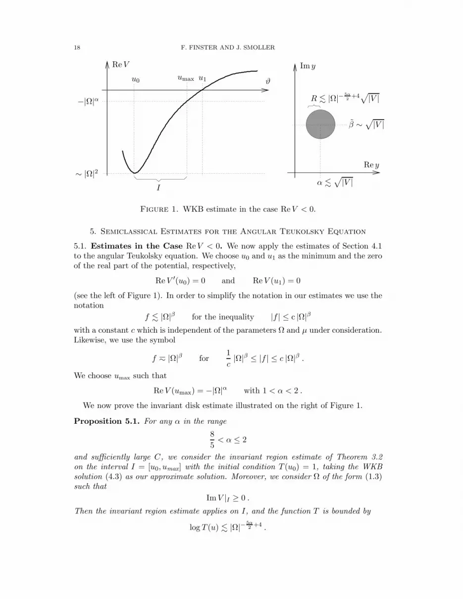
Figure 1. WKB estimate in the case ReV < 0.

5. Semiclassical Estimates for the Angular Teukolsky Equation

5.1. Estimates in the Case ReV < 0. We now apply the estimates of Section 4.1to the angular Teukolsky equation. We choose u0 and u1 as the minimum and the zeroof the real part of the potential, respectively,

ReV ′(u0) = 0 and ReV (u1) = 0

(see the left of Figure 1). In order to simplify the notation in our estimates we use thenotation

f . |Ω|β for the inequality |f | ≤ c |Ω|β

with a constant c which is independent of the parameters Ω and µ under consideration.Likewise, we use the symbol

f h |Ω|β for1

c|Ω|β ≤ |f | ≤ c |Ω|β .

We choose umax

such that

ReV (umax) = −|Ω|α with 1 < α < 2 .

We now prove the invariant disk estimate illustrated on the right of Figure 1.

Proposition 5.1. For any α in the range

8

5< α ≤ 2

and sufficiently large C, we consider the invariant region estimate of Theorem 3.2on the interval I = [u0, umax] with the initial condition T (u0) = 1, taking the WKBsolution (4.3) as our approximate solution. Moreover, we consider Ω of the form (1.3)such that

ImV |I ≥ 0 .

Then the invariant region estimate applies on I, and the function T is bounded by

log T (u) . |Ω|− 5α

2+4 .


u0 umin

ϑ

ReV

u1

α+√U

α h ReV

Re y

β +R h |Ω|2− 3α

2

√

|V |Im y

β +R

h |Ω|1− 3α

4

√

|V |I

C |Ω|α

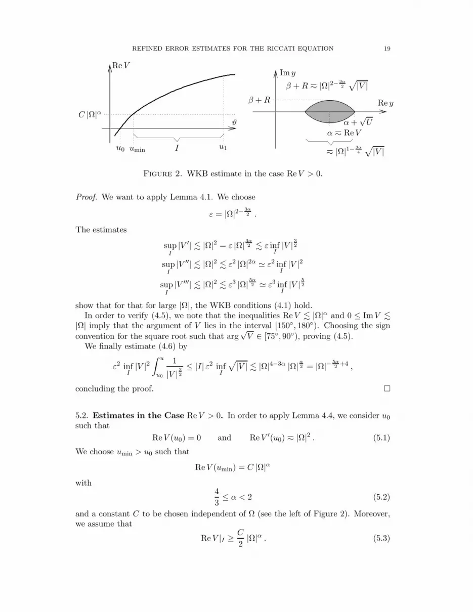
Figure 2. WKB estimate in the case ReV > 0.

Proof. We want to apply Lemma 4.1. We choose

ε = |Ω|2− 3α

2 .

The estimates

supI

|V ′| . |Ω|2 = ε |Ω| 3α2 . ε infI|V | 32

supI

|V ′′| . |Ω|2 . ε2 |Ω|2α ≃ ε2 infI|V |2

supI

|V ′′′| . |Ω|2 . ε3 |Ω| 5α2 ≃ ε3 infI|V | 52

show that for that for large |Ω|, the WKB conditions (4.1) hold.In order to verify (4.5), we note that the inequalities ReV . |Ω|α and 0 ≤ ImV .

|Ω| imply that the argument of V lies in the interval [150, 180). Choosing the sign

convention for the square root such that arg√V ∈ [75, 90), proving (4.5).

We finally estimate (4.6) by

ε2 infI|V |2

∫ u

u0

1

|V | 32≤ |I| ε2 inf

I

√

|V | . |Ω|4−3α |Ω|α2 = |Ω|− 5α

2+4 ,

concluding the proof.

5.2. Estimates in the Case ReV > 0. In order to apply Lemma 4.4, we consider u0such that

ReV (u0) = 0 and ReV ′(u0) h |Ω|2 . (5.1)

We choose umin > u0 such that

ReV (umin) = C |Ω|α

with4

3≤ α < 2 (5.2)

and a constant C to be chosen independent of Ω (see the left of Figure 2). Moreover,we assume that

ReV |I ≥C

2|Ω|α . (5.3)


We next apply the invariant region estimates of Proposition 3.5, relying on the esti-mates of Lemmas 4.4 and 4.5. We introduce the set I as the intersection of the upperhalf plane with the circle with center m = α+ iβ and radius R,

I = z ∈ C | |z −m| ≤ R and Re z ≥ 0(where again α = Re y and y as in (4.18) and (4.16)). Moreover, we let I be thecomplex conjugate of the set I.

Proposition 5.2. We choose the interval I = [umin, u1] according to (5.1)–(5.3).Assume that that V satisfies on I the conditions (4.1) and (4.21). Then the region I∪Iis invariant under the Riccati flow. Moreover,

R+ β h |Ω|2− 3α

2

√

|V | , |R2 − β2| . |Ω|2− 3α

2 |V | . (5.4)

Before giving the proof, we note that in the case U < 0, the sets I and I do notintersect, so that the invariant region are two disjoint disks. In the case U > 0, thetwo disks form a connected set. In the case β < 0, we obtain a lens-shaped invariantregion, as as illustrated on the right of Figure 2.

Proof of Proposition 5.2. Similar as in the proof of Proposition 5.1, a Taylor expansionof the potential around u0 yields that

umin − u0 h |Ω|α−2 .

We want to choose ε as small as possible, but in agreement with (4.1). This leads usto make the ansatz

ε = δ |Ω|2− 3α

2

with 0 < δ ≪ 1 independent of |Ω|. By choosing δ sufficiently small and C sufficientlylarge, we can arrange that the inequalities (4.1), (4.20) as well as the last inequalityin (4.32) hold. Next we choose ν in agreement with (4.32), but as small as possible,

ν = 20 δ |Ω|2− 3α

2 .

Let us verify that Lemmas 4.4 and 4.5 apply. As just explained, (4.20) holds forsufficiently small δ. According to (1.3), we know that

|Ω| & | ImV | = 2Re√V Im

√V

and thus in view of (5.3),

Re√V & C

1

2 |Ω|α2 and∣

∣ Im√V∣

∣ . C− 1

2 |Ω|1−α

2 . (5.5)

Thus, possibly after increasing C, the inequality (4.21) is satisfied. Hence Lemma 4.4applies. The inequalities (4.32) again hold for sufficiently small δ. Using (5.5), we seethat

∣

∣

∣

∣

∣

Im√V

Re√V

∣

∣

∣

∣

∣

. C−1 |Ω|1−α =ν

10

|Ω|−1+α

2

2δ C,

and in view of (5.2), the last factor can be made arbitrarily small by further increas-ing C if necessary. Hence (4.33) holds, and Lemma 4.5 applies.

We begin with the case when y lies in the upper half plane (the general case will betreated below). Choosing s = 1, we can apply Proposition 3.5 to obtain the invariantregion estimate (3.30). The first inequality in (5.4) follows from the first equation


in (3.30) and (4.34). Similarly, the second inequality in (5.4) follows from the secondequation in (3.30) and (4.22), noting that according to (5.5),

Im2√V . |Ω|2−α . |Ω|2−2α |V | . ε|V | .

If y lies in the lower half plane, we take the complex conjugate of the Riccati equationand again apply the above estimates. This simply amounts to flipping the sign of βin all formulas. If y(u) crosses the real line, we can perform the replacement β → −β,which describes a reflection of the invariant circle at the real axis. In this way, we canflip from estimates in the upper to estimates in the lower half plane and vice versa,without violating our estimates. We conclude that y stays inside the lens-shaped regionobtained as the intersection of the two corresponding invariant circles.

6. Parabolic Cylinder Estimates

Near the turning points of the real part of the potential, we approximate the po-tential by a quadratic polynomial,

V (u) = p+q

4(u− r)2 with p, q, r ∈ C . (6.1)

The corresponding differential equation (3.12) can be solved explicitly in terms of theparabolic cylinder function, as we now recall. The parabolic cylinder function, whichwe denote by Ua(z), is a solution of the differential equation

U ′′a (z) =

(z2

4+ a)

Ua(z) .

Setting

φ(u) = Ua(z) with a =p√q, z = q

1

4 (u− r) , (6.2)

a short calculation shows that φ indeed satisfies (3.12). We set

b = −4(

a− 1

2

)

.

6.1. Estimates of Parabolic Cylinder Functions. In preparation for getting in-variant region estimates, we need to get good control of the parabolic cylinder func-tion Ua(z). To this end, in this section we elaborate on the general results in [9] andbring them into a form which is most convenient for our applications.

Lemma 6.1. There is a constant c > 0 such that for all parameters z, b in the range

|z|2 > c and |z|2 > 4|b| ,the parabolic cylinder function is well-approximated by the WKB solution.

Proof. We want to apply [9, Theorem 3.3] in the case t0 = t+ (with t+ as defined in [9,eqn (3.10)]). Using [9, eqns (3.14) and (3.17)], we find

|8d| ≥∣

∣

∣z +

√

z2 − b∣

∣

∣

2≥∣

∣

∣2√

|b|+√

3|b|∣

∣

∣

2= (2 +

√3)2 |b| > 8 |b| .

Hence the parameter ρ defined in [9, eqn (3.17)]) is smaller than 1/8, making it possibleto choose κ = 1/4 (see [9, Lemma 3.2]). Applying [9, Theorem 3.3] gives the result.

For the following estimates, we work with the Airy-WKB limit, giving us the as-ymptotic solution [9, eqns (3.36) and (3.37)].


Lemma 6.2. Assume that

|z2 − b| ≤ |b| 13 , arg b ∈ (88, 92) and |b| > 100 .

Then the estimate of [9, Theorem 3.9] applies and |h(z)|2 < 2.

Proof. According to [9, eqns (3.10) and (3.37)]

4t20 − b = 2(z2 − b)± 2z√

z2 − b

|h(z)|2 =1

4·2 4

3

|b|− 4

3 |4t20 − b|2

and thus

|z|2 ≤ |z2 − b|+ |b| ≤ |b|+ |b| 13

|z| ≤ |b| 12 + |b| 16∣

∣z ±√

z2 − b∣

∣ ≤ |z|+ |b| 13 ≤ |b| 12 + 2 |b| 16∣

∣z ±√

z2 − b∣

∣

2 ≤ |b|+ 8 |b| 23

|4t20 − b|2 ≤ 4 |z2 − b|∣

∣

∣z ±

√

z2 − b∣

∣

∣

2

≤ 4 |b| 43(

1 + 8 |b|− 1

3

)

|h(z)|2 ≤ 1

24

3

(

1 + 8 |b|− 1

3

)

< 2

∣

∣

∣

∣

4t20b

− 1

∣

∣

∣

∣

2

≤ 4 |b|− 2

3

(

1 + 8 |b|− 1

3

)

< 0.6 . (6.3)

We now apply [9, Theorem 3.9], noting that (6.3) implies the condition [9, eqn (3.39)].

Lemma 6.3. For any c > 0 there is a constant C > 0 such that the following statementis valid. Assume that

|z2 − b| > |b| 13 , |Re z2|, |Re b| < c and Im z2, Im b > C .

Then the assumptions of [9, Theorem 3.9] hold. Moreover, the argument h2 of the Airyfunction in [9, eqn (3.36)] avoids the branch cut (i.e. there is a constant ε(c,C) > 0such that [9, eqn (2.6)] holds). As a consequence, the Airy function has the WKBapproximation given in [9, Theorem 2.2].

Proof. By choosing C sufficiently large, we can arrange that the arguments of z2 and bare arbitrarily close to 90. Moreover, as shown in Figure 3, we have the inequality

cos arg(z2 − b) ≤ 2c

|z2 − b| ≤ 2c |b|− 1

3 ≤ 2cC− 1

3 ,

showing that for sufficiently large C, the argument of z2−b is arbitrarily close to ±90.We next consider the phase of t0 given by either t+ or t−,

t0 =1

2

(

z ±√

z2 − b)

. (6.4)

We need to consider both signs in order to take into account both branches of thesquare root. Since the arguments of both z2 and z2 − b are arbitrarily close to 90, we


c

b

z2

−c

Figure 3. Estimating the argument of z2 − b.

know that the arguments of z and√z2 − b are both arbitrarily close to 45mod 180.

Hence choosing the sign in (6.4) such that the real parts of z and ±√z2 − b have

the signs, it follows immediately that the argument of t0 is also arbitrarily close to 45

mod 180. The identity

t+ t− =b

4yields that for sufficiently large C, the argument of the other branch is also arbitrarilyclose to 45mod 180.

As a consequence, the conditions [9, eqns (3.38) and (3.39)] are satisfied. Moreover,the phase r in [9, Section 3.4] takes the values

3r := arg

(

− b

t30

)

≈ 135 mod 180 ,

with an arbitrarily small error. Since r must be chosen in the interval (−60, 0) (see [9,eqn (3.35)]), we conclude that

r ≈ −15 .

Next, we consider the phase of the function h(z), which we write as

h(z) = ±2e−2ir

22

3

|t0|2t20

|b|− 2

3

√

z2 − b t0 .

It follows that

arg h(z) ≈ −2r mod 180 ≈ 30 mod 180 ,

and thus arg(h(z)2) ≈ 60. This shows that the argument of the Airy function in [9,eqn (3.36)] does indeed avoid the branch cut.

Lemma 6.4. For any c > 0, there are positive constants C1 and C2 such that forsufficiently large |Ω|, the following statement holds. We consider the quadratic poten-tial (6.1) with parameters p, q and r in the range

|pq| ≥ C1 |Ω|3 (6.5)

|Re p| ≥ C1 |Ω| , | Im p| ≤ c |Ω| (6.6)

|Re q| ≤ c |Ω|2 , | Im q| ≤ c |Ω| (6.7)

|Re r| ≤ c , | Im r| ≤ c |Ω|−1 . (6.8)


We choose φ(u) = U+a (z(u)) as the parabolic cylinder function defined by the con-

tour Γ+ = R + i (see [9, eqn (3.2)]) and let y = φ′(u)/φ(u) be the corresponding

solution of the Riccati equation. We denote the zero of Re V by u1 and set

u± = u1 ± C2 |pq|−1

6 . (6.9)

Assume that z and b given by (6.2) are in the range

Im z2, Im b > C2 .

Then for all u ∈ [0,Re r] we have the estimates

|Re y| ≤ |Re√

V |+ C1 |pq|1

6 (6.10)

| Im y| ≤∣

∣ Im√

V∣

∣+ C1 |pq|1

6 (6.11)

1

2

∣

∣ Im√

V∣

∣ ≤ − Im y if u < u− . (6.12)

Proof. Using the scaling of the parameters p, q and r, we find

|u1 − r| ≃∣

∣

∣

∣

p

q

∣

∣

∣

∣

1

2

V ′(u1) =q

2(u1 − r) ≃ |pq| 12

V ′(u1) (u+ − u−) ≃ C2 |pq|1

3

V ′′(u1) (u+ − u−)2 ≃ |q| C2

2 |pq|− 1

3 = C22 |pq| 13

∣

∣

∣

∣

q

p2

∣

∣

∣

∣

1

3

In view of (6.6) and (6.7), the quotient q/p2 can be made arbitrarily small by increas-ing C1. This makes it possible to arrange that on the interval [u−, u+], the dominant

term in V is the linear term. As a consequence,

V (u−) ≃ V ′(u1) (u− − u1) ≃ C2 |pq|1

3 (6.13)

z2 − b = q1

2 (u− r)2 + 4p√q+ 2 =

4√qV + 2 (6.14)

z(u−)2 − b ≃ C2 |p|

1

3 |q|− 1

6 = C2 |b|1

3 . (6.15)

Hence at u−, Lemma 6.3 shows that the WKB approximation applies. Possibly by

increasing C2, we can arrange that y = ±√

V with an arbitrarily small relative error.Clearly, this WKB estimate also holds for u < u− and for u > u+.

In order to justify the sign in (6.12), we choose the square roots such that

arg z ≈ 45 , arg q1

4 ≈ 135 .

Then the WKB estimate of [9, Theorem 3.3; see also eqn (3.30)] shows that thefunction U+

a is approximated by

Ua(z) ∼ exp

(√z

4

√

z2 − b

)

,

where the sign of the square root is chosen such that

arg√

z2 − b ≈ 45 if u < u− and arg√

z2 − b ≈ −45 if u > u+ .


As a consequence,

y(u) ≃ d

du

(√z

4

√

z2 − b

)

=1

4

2z2 − b√z2 − b

q1

4 .

A short calculation shows that

Im y(u) < 0 if u < u− and Re y(u) > 0 if u > u+ .

It remains to estimate y on the interval [u−, u+]. If this interval does not inter-sect [0,Re r], there is nothing to do. If this intersection is not empty and u− 6∈ [0,Re r],we replace r by r + 1. Thus we may assume that u− ∈ [0,Re r]. In view of (6.9)and (6.13), we know that

max[u

−,u+]

√

|V | (u+ − u−) ≃ C23

2 .

Hence we can apply Lemma 3.7 to y to obtain

| Im y(u)| ≥ 1

c2| Im y(u)| − c2 (u+ − u−) max

[u−,u+]

| ImV |

with a constant c2 which depends only on C2. From our assumption (6.6)–(6.8) itfollows that | ImV | ≤ c′|Ω|, where c′ depends only on c. Moreover, at u− we can usethe WKB estimate together with (6.13). Also applying (6.9), we obtain

| Im y(u)| ≥ 1

c22|pq| 16

(

1− 2 c′ c22 |Ω| |pq|−1

3

)

.

In view of (6.5), by increasing C1 we can arrange that the first summand dominatesthe second, meaning that

| Im y(u)| ≥ 1

2c22|pq| 16 .

Increasing C1 if necessary, we obtain the result.

We finally remark that it is a pure convention of the parabolic cylinder functionsdefined in [9] that y lies in the lower half plane. Solutions in the upper half plane arereadily obtained with the following double conjugation method: We consider the solu-

tion U+a (z) corresponding to the complex conjugate potential V . Then φ(u) := Ua(z)+

is a parabolic cylinder function corresponding to the potential V . The correspondingRiccati solution y(u) := φ′(u)/φ(u) satisfies (6.10), (6.11) and, in analogy to (6.12),the inequality

1

2

∣

∣ Im√

V∣

∣ ≤ Im y if u < u− . (6.16)

6.2. Applications to the Angular Teukolsky Equation. We now want to getestimates on an interval I = [umin, umax

] which includes a zero of ReV , which wedenote by u1. We choose

V (u) = V (u1) + V ′(u1) (u− u1) +1

2V′′ (u− u1)

2

with

V′′ := i ImV ′′(u1) + max

IReV ′′ .

We define u± as in Lemma 6.4.


Lemma 6.5. Assume that ImV ≥ 0 on the interval [umin, u+] and that the assump-tions of Lemma 6.4 hold. Moreover, assume that for sufficiently large |Ω|,

|V (u)| & |Ω|2 (u− u1)2 . (6.17)

Then for sufficiently large |Ω|, the invariant region estimate of Theorem 3.3 applieswith g ≡ 0 and

log T∣

∣

u

umin≤ C (u− umin) for all u ∈ [umin, u−] ,

where the constant C is independent of Ω.

Proof. We take V as the approximate potential. As the approximate solution y of thecorresponding Riccati equation, we take the the double conjugate solution introducedbefore (6.16).

The function f := Re(V − V ) has the properties

f(u1) = 0 = f ′(u1) and f ′′(u) ≤ 0 on I .

Thus it is concave and lies below any tangent. In particular, it is everywhere negative,

Re(V − V ) ≤ 0 .

Hence (3.17) gives

U ≤ −β2 .

We now estimate the error terms E1, E2, E3 in Theorem 3.3:

∫ u

umin

|E1| .∫ u

umin

1

β(v)2

(

|α(v)| |Re(V − V )|+ |Re(V − V )′|)

dv

.

∫ u

umin

1

β(v)2

(

|α(v)| |Ω|2 |v − u1|3 + |Ω|2 |v − u1|2)

dv

. |Ω|2∫ u

umin

(

αβ

β3|v − u1|3 +

|v − u1|2β2

)

dv .

Applying Lemma 6.4 gives

. |Ω|2∫ u

umin

( | Im V ||V | 32

|v − u1|3 +|v − u1|2

|V |

)

dv .

We now apply (6.17) and use that | Im V | . |Ω| to obtain

. |Ω|2∫ u

umin

( |Ω||Ω|3 +

1

|Ω|2)

dv . u− umin .


Similarly,∫ u

umin

|E2| .∫ u

umin

1

|β|| Im(V − V )| dv .

∫ u

umin

1

|β||Ω| |v − u1|3 dv

.

∫ u

umin

|v − u1|2 dv . u− umin

∫ u

umin

|E3| .∫ u

umin

| ImV ||β|3

|Re(V − V )| dv

. |Ω|3∫ u

umin

|v − u1|3

|V | 32dv . u− umin .

This completes the proof.

7. Estimates for a Singular Potential

At u = 0, the potential (2.3) has a pole of the form

V (u) =

(

(k − s)2 − 1

4

)

1

u2+ O(u0) .

In preparation for estimating the solutions near this pole (see Section 8 below), in thissection we analyze solutions of the Riccati equation for a potential includes the poleand involves a general constant. More precisely, setting L = |k − s|, we consider apotential of the form

V (u) =

(

L2 − 1

4

)

1

u2+ ζ2 (7.1)

for a complex parameter ζ and a non-negative integer L. In the case L = 0, the realpart of V tends to −∞ as u ց 0, whereas in the case L > 0, it tends to +∞. We treatthese two cases separately.

7.1. The case L = 0. In this case, the potential (7.1) becomes

V (u) = − 1

4u2+ ζ2 . (7.2)

We assume that ζ lies in the upper right half plane excluding the real axis,

arg ζ ∈ (0, 90] .

The corresponding Sturm-Liouville equation (3.12) has explicit solutions in terms ofthe Bessel function K0 and I0 (see [12, §10.2.5]). We choose

φ(u) = −√u(

K0(ζu) +(

arg ζ − log(2) + γ + i)

I0(ζu))

(7.3)

(where γ ≈ 0.577 is Euler’s constant). Near the origin, we have the asymptotics [12,eq. (10.31.2)]

φ(u) =√u log |ζu|+ i

√u+ O(u) .

For large u, on the other hand, we have the asymptotics (see [12, §10.40(i)])

φ(u) = − eζu√2πζ

(

arg ζ − log(2) + γ + i) (

1 + O(

(ζu)−1))

.

We again denote the corresponding solution of the Riccati equation by y = φ′/φ.


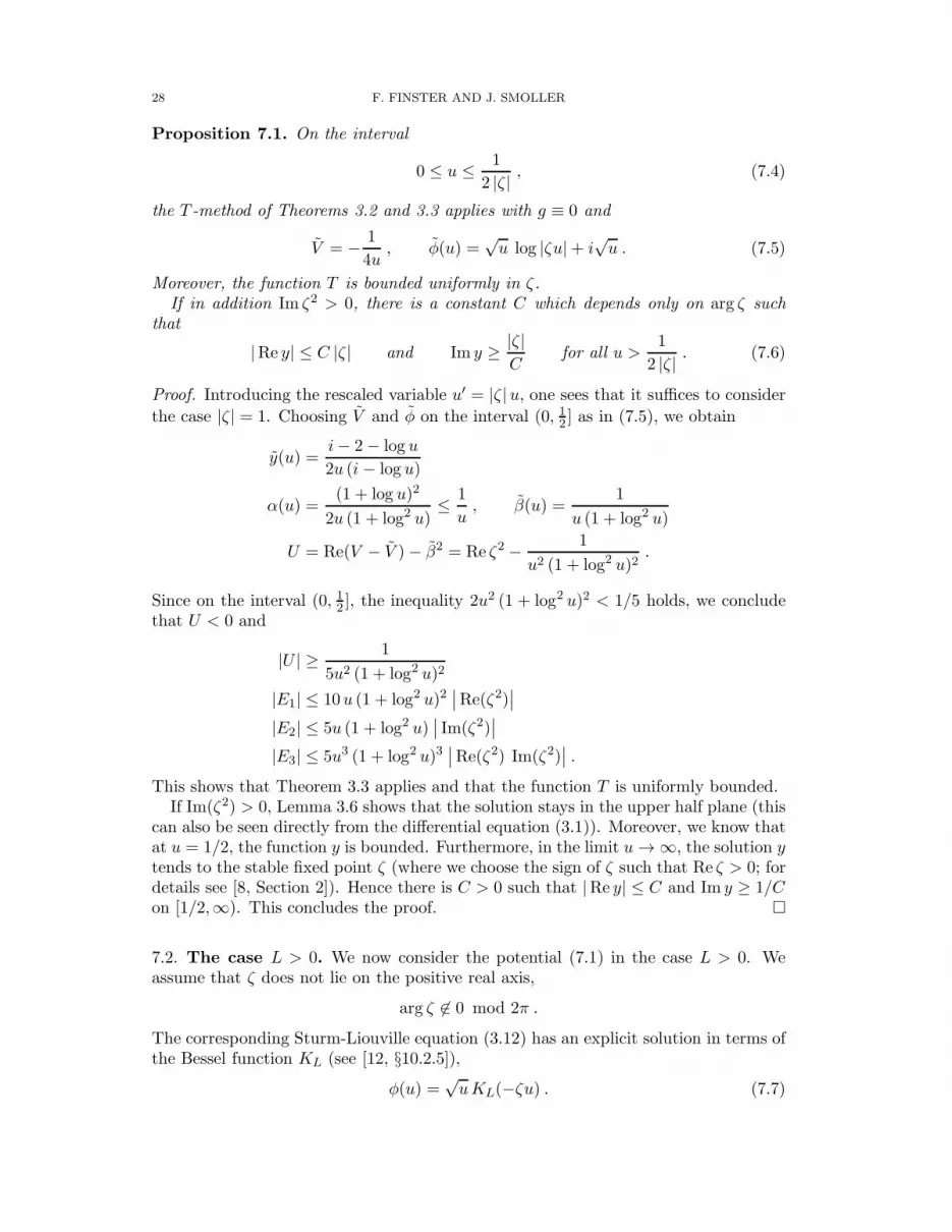
Proposition 7.1. On the interval

0 ≤ u ≤ 1

2 |ζ| , (7.4)

the T -method of Theorems 3.2 and 3.3 applies with g ≡ 0 and

V = − 1

4u, φ(u) =

√u log |ζu|+ i

√u . (7.5)

Moreover, the function T is bounded uniformly in ζ.If in addition Im ζ2 > 0, there is a constant C which depends only on arg ζ such

that

|Re y| ≤ C |ζ| and Im y ≥ |ζ|C

for all u >1

2 |ζ| . (7.6)

Proof. Introducing the rescaled variable u′ = |ζ|u, one sees that it suffices to consider

the case |ζ| = 1. Choosing V and φ on the interval (0, 12 ] as in (7.5), we obtain

y(u) =i− 2− log u

2u (i − log u)

α(u) =(1 + log u)2

2u (1 + log2 u)≤ 1

u, β(u) =

1

u (1 + log2 u)

U = Re(V − V )− β2 = Re ζ2 − 1

u2 (1 + log2 u)2.

Since on the interval (0, 12 ], the inequality 2u2 (1 + log2 u)2 < 1/5 holds, we concludethat U < 0 and

|U | ≥ 1

5u2 (1 + log2 u)2

|E1| ≤ 10u (1 + log2 u)2∣

∣Re(ζ2)∣

∣

|E2| ≤ 5u (1 + log2 u)∣

∣ Im(ζ2)∣

∣

|E3| ≤ 5u3 (1 + log2 u)3∣

∣Re(ζ2) Im(ζ2)∣

∣ .

This shows that Theorem 3.3 applies and that the function T is uniformly bounded.If Im(ζ2) > 0, Lemma 3.6 shows that the solution stays in the upper half plane (this

can also be seen directly from the differential equation (3.1)). Moreover, we know thatat u = 1/2, the function y is bounded. Furthermore, in the limit u → ∞, the solution ytends to the stable fixed point ζ (where we choose the sign of ζ such that Re ζ > 0; fordetails see [8, Section 2]). Hence there is C > 0 such that |Re y| ≤ C and Im y ≥ 1/Con [1/2,∞). This concludes the proof.

7.2. The case L > 0. We now consider the potential (7.1) in the case L > 0. Weassume that ζ does not lie on the positive real axis,

arg ζ 6∈ 0 mod 2π .

The corresponding Sturm-Liouville equation (3.12) has an explicit solution in terms ofthe Bessel function KL (see [12, §10.2.5]),

φ(u) =√uKL(−ζu) . (7.7)


-2.0 -1.5 -1.0 -0.5Re y

-1.0

-0.5

Im y

Figure 4. The Bessel solution y for ζ = −1, ζ = −i and ζ = exp(−75 iπ/180).

Using the recurrence relations in [12, eqs. (10.29.2) and (10.29.1)], it follows that

y(u) =1− 2L

u+ ζ

KL−1(−ζu)

KL(−ζu). (7.8)

Near the origin, we have the asymptotics (see [12, eqs. (10.31.1) and (10.25.2)])

φ(u) =(n− 1)!√

2ζ

(

−ζu

2

)1

2−L

(1 + O(u)) −√2

L!√ζ

(

ζu

2

)1

2+L

(1 + O(u)) ,

whereas for large u, we have the asymptotics (see [12, eq. (10.25.3)])

φ(u) ∼√

− π

2ζeζu , y(u) ∼ ζ as u → +∞

(where the square root is taken such that Re√−ζ > 0).

Proposition 7.2. For sufficiently small ε > 0, the following statement holds: If theargument of ζ lies in the range

arg ζ ∈(

180 − ε, 180 + ε)

∪(

− 90 − ε, 90 + ε)

∪(

− 75 − ε, 75 + ε)

, (7.9)

then the Bessel solution (7.8) satisfies for all u ∈ R+ the inequalities

|y(u)| ≥ |ζ|4

and 150 < arg y(u) < 300 . (7.10)

Proof. Rescaling the variables by |ζ|u → u, we may assume that |ζ| = 1. The solutionsfor ζ = −1, ζ = −i and ζ = exp(−75 iπ/180) satisfy (7.10), as one sees from Figure 4.The result now follows by continuity.

8. Estimates for the Angular Teukolsky Equation near the Poles

Near u = 0, the potential (2.3) has the expansion

V (u) =

(

L2 − 1

4

)

1

u2+ c0 + c2u

2 + O(Ω2u4) ,

where we again set L = |k − s|, and where the coefficients c0 and c2 scale in Ω like

c0 = −2sΩ− µ+ O(Ω0) , c2 = Ω2 + O(Ω) . (8.1)


We again treat the cases L = 0 and L > 0 separately.

8.1. The Case L = 0. Our goal is to estimate the solutions on an interval I :=(0, u

max]. We choose the approximate potential according to (7.2),

V (u) = − 1

4u2+ ζ2 ,

and take (7.3) as the solution φ of the corresponding Sturm-Liouville equation (3.12).The constant ζ in (7.1) is chosen as

Im ζ2 = Im c0 and Re ζ2 = maxI

Re

(

V (u)−(

L2 − 1

4

) 1

u2

)

.

Then by construction we have Re(V − V ) ≤ 0. In view of (3.17), we conclude that Uis negative, making it possible to apply the T -method. Moreover,

|U | ≥ β2 , |U | ≥ 2β

√

Re(V − V ) (8.2)

|Re(V − V )| . |Ω|2 u2max

, |Re(V − V )′| . |Ω|2 umax

(8.3)

| Im(V − V )| . |Ω| u2 (8.4)

Proposition 8.1. Assume that Im ζ2 > 0. We consider the solution φ on the interval

(0, umax

] with umax

. |Ω|− 1

2 , (8.5)

having the following asymptotics near u = 0,

φ(u) =√u log |ζu|+ i

√u+ O(u) .

Then the T -estimates of Theorems 3.2 and 3.3 apply with g ≡ 0 and

log T (u) ≤ C |Ω|u2max

(

1 + log4 |ζu|)

for all u ∈ (0, umax

] .

Here

C is a numerical constant if umax

≤ (2|ζ|)−1

C depends on arg ζ if umax

> (2|ζ|)−1 .

Proof. The function φ coincides with the function φ in Proposition 7.1. Hence on theinterval (7.4), we obtain, for a suitable numerical constant c,

|α| ≤ c

u, |β| ≥ 1

cu (1 + log2|ζu|)

|E1| ≤2c3

uu2 (1 + log2|ζu|)2 |Re(V − V )|+ c2u2

2(1 + log2|ζu|)2 |Re(V − V )′|

(8.3)

.(

2c3 +c2

2

)

|Ω|2 u3max

(1 + log2|ζu|)2

|E2| ≤1

β| Im(V − V )|

(8.4)

. c |Ω| u3 (1 + log2|ζu|)

|E3| ≤| ImV |β3

|Re(V − V )|(8.3)

. c3 |Ω|3 u3u2max

(1 + log2|ζu|)2 .

In the remaining region u > 1/(2|ζ|), we know in view of (8.5) that

|ζ| & |Ω| 12 . (8.6)


We have the global estimates (7.6) for α and β. Using the second inequality in (8.2),we can estimate the error terms by

|E1| ≤α

β

√

Re(V − V ) +|Re(V − V )′|

β2

. C2 |Ω|umax

+C2

|ζ|2 |Ω|2 umax

(8.6)

. C2 |Ω|umax

|E2| ≤| Im(V − V )|

|β|.

C|Ω||ζ|

(8.6)

. C |Ω| 12

|E3| ≤| ImV |β3

|Re(V − V )| . C3

|ζ|3 |Ω|3 u2max

(8.6)

. C3 |Ω| 32 u2max

.

Integrating the error terms from u to umax

, using (8.5) and renaming the constantsgives the result.

8.2. The Case L > 0. We choose u0 such that

ReV ′(u0) = 0 .

According to (8.1), we know that

u0 ≃ |Ω|− 1

2 . (8.7)

Our goal is to estimate the solutions on the interval I := (0, u0]. We take (7.1) as ourapproximate potential

V =

(

L2 − 1

4

)

1

u2+ ζ2 , (8.8)

where

ζ2 = c0 − (1 + 2i) C2 |Ω| , (8.9)

and C is a constant to be determined later. Then

V − V = (1 + 2i) C2 |Ω|+ c2u2 + O(Ω2u4) . (8.10)

We choose a constant

c3 ≥1

|Ω| sup(0,u0]

∣

∣

∣V − V − (1 + 2i) C2 |Ω|

∣

∣

∣. (8.11)

In view of (8.1) and (8.7), the constant c3 can indeed be chosen independent of Ω.

Lemma 8.2. For every Cmin > 0 there is Cmax such that for every c0 with

| Im c0| . |Ω| , (8.12)

there is a parameter C in the range

Cmin ≤ C ≤ Cmax

and a complex number ζ which satisfies (8.9), such that the conditions in Proposi-tion (7.2) hold.


Proof. In the limit |c0| → ∞, the real part of c0 dominates its imaginary part in viewof (8.12). Thus taking C = Cmin, the argument of ζ2 tends to zero or π as |c0| → ∞.Taking the square root, we can thus satisfy (7.9). More precisely, there is a constant c4(independent of Ω) such that (7.9) holds if |c0| > c4 |Ω|.

In the remaining case |c0| ≤ c4 |Ω|, we choose C = Cmax. By choosing Cmax ≫ c4, wecan arrange that the argument of ζ2 lies arbitrarily close to arg(−(1+ 2i). Taking thesquare root, we see that (7.9) again holds.

We are now in a position to apply the κ-method of Proposition 3.5. We choose theapproximate potential (8.8) with ζ in agreement with Lemma 8.2. Moreover, we choose

the solution φ of the corresponding Sturm-Liouville equation (3.12) to be the Bessel

solution (7.7). Again, we denote the corresponding Riccati solution by y = φ′/φ. Ithas the properties

|y| ≥ C4|Ω| 12 (8.13)

and

150 < arg y < 300 . (8.14)

Proposition 8.3. Choosing the function g in (3.29) as

g(u) = C2 |Ω| 12 σ(u) , (8.15)

and choosing C sufficiently large (independent of Ω), the disks defined by (3.30) areinvariant under the backward Riccati flow. Moreover, the determinator D is positive.

Proof. We want to apply Proposition 3.5 starting at u0 going backwards to the sin-gularity at the origin. Up to now, we always applied the invariant region estimatesfor increasing u. In order to avoid confusion, we now replace u by −u, so that weneed to estimate the solution on the interval [−u0, 0) (note that the potential in theSturm-Liouville equation does not change sign under the change of variables u → −u).

Since the relation y = φ′/φ involves one derivative, the function y changes sign, sothat (8.14) becomes

− 30 ≤ arg y ≤ 120 . (8.16)

Using (8.10) and (8.11), we obtain

|Re(V − V )′| . |Ω|2|u| . |Ω| 32 (8.17)

2αRe(V − V ) ≥ 2α C2 |Ω| − 2α c3 |Ω|β Im(V − V ) ≥ 2β C2 |Ω| − β c3 |Ω| .

Adding the last two inequalities and using the trigonometric bound

α+ β =

⟨(

11

)

,

(

α

β

)⟩

(8.16)

≥√2 |y| cos 75 ≥ 1

3|y| ,

we get

2αRe(V − V ) + β Im(V − V ) ≥ 2

3|y| C2 |Ω| − 3 |y| c3 |Ω|

=2

3|y| (C2 − 5c3) |Ω|

(8.13)

≥ C6(C2 − 5c3) |Ω|

3

2 .


By choosing C sufficiently large (independent of |Ω|), we can arrange that

2αRe(V − V ) + β Im(V − V ) ≥ C3

8|Ω| 32 . (8.18)

Note that the function g in (8.15) is monotone increasing because of (3.4) and (8.16).Moreover,

κ = C2 |Ω| 12 +1

σ

∫ u

u0

σ Im(V − V ) .

Using (8.10) and (8.11) together with the fact that σ is monotone increasing, weconclude that

C2 |Ω| 12 − c3∣

∣Ωu0∣

∣ ≤ κ ≤ C2(

|Ω| 12 + |Ωu0|)

+ c3∣

∣Ωu0∣

∣ .

Using (8.7), possibly by increasing C we can arrange that

C2

2|Ω| 12 ≤ κ ≤ 2 C2 |Ω| 12 .

We now estimate κ−R using Lemma 3.28. Keeping in mind that β ≥ 0, we obtain

|Re(V − V )||β + κ|

≤ 2(C2 + c3)

C2|Ω| 12

κ2

|β + κ|≤ κ ≤ 2 C2 |Ω| 12 .

Thus, possibly after increasing C, we obtain

|κ−R| ≤ 2 C2 |Ω| 12 .

As a consequence,

|(κ−R) ImV | . 2 C2 |Ω| 32 . (8.19)

Comparing (8.18) with (8.17) and (8.19), one sees that, possibly by further in-creasing C, we can arrange that the determinator as given by (3.27) is positive. Thisconcludes the proof.

Acknowledgments: We are grateful to the Vielberth Foundation, Regensburg, for gen-erous support.

References

[1] L. Andersson and P. Blue, Uniform energy bound and asymptotics for the Maxwell field on a

slowly rotating kerr black hole exterior, arXiv:1310.2664 [math.AP] (2013).[2] S. Chandrasekhar, The Mathematical Theory of Black Holes, Oxford Classic Texts in the Physical

Sciences, The Clarendon Press Oxford University Press, New York, 1998.[3] S. Dyatlov, Asymptotic distribution of quasi-normal modes for Kerr–de Sitter black holes,

arXiv:1101.1260 [math.AP], Ann. Henri Poincare 13 (2012), no. 5, 1101–1166.[4] F. Finster, N. Kamran, J. Smoller, and S.-T. Yau, An integral spectral representation of the

propagator for the wave equation in the Kerr geometry, gr-qc/0310024, Comm. Math. Phys. 260(2005), no. 2, 257–298.

[5] F. Finster and H. Schmid, Spectral estimates and non-selfadjoint perturbations of spheroidal wave

operators, J. Reine Angew. Math. 601 (2006), 71–107.[6] F. Finster and J. Smoller, A spectral representation for spin-weighted spheroidal wave operators

with complex aspherical parameter, in preparation.[7] , Decay of solutions of the Teukolsky equation for higher spin in the Schwarzschild geom-

etry, arXiv:gr-qc/0607046, Adv. Theor. Math. Phys. 13 (2009), no. 1, 71–110.

http://arxiv.org/abs/1310.2664


http://arxiv.org/abs/gr-qc/0310024

http://arxiv.org/abs/gr-qc/0607046


[8] , Error estimates for approximate solutions of the Riccati equation with real or complex

potentials, arXiv:0807.4406 [math-ph], Arch. Ration. Mech. Anal. 197 (2010), no. 3, 985–1009.[9] , Absence of zeros and asymptotic error estimates for Airy and parabolic cylinder functions,

arXiv:1207.6861 [math.CA], Commun. Math. Sci. 12 (2014), no. 1, 175–200.[10] C. Flammer, Spheroidal Wave Functions, Stanford University Press, Stanford, California, 1957.[11] J.N. Goldberg, A.J. Macfarlane, E.T. Newman, F. Rohrlich, and E.C.G. Sudarshan, Spin-s spher-

ical harmonics and ∂, J. Math. Phys. 8 (1967), 2155–2161.[12] F.W.J. Olver, D.W. Lozier, R.F. Boisvert, and C.W. Clark (eds.), Digital Library of Mathematical

Functions, National Institute of Standards and Technology from http://dlmf.nist.gov/ (releasedate 2011-07-01), Washington, DC, 2010.

[13] S.A. Teukolsky, Perturbations of a rotating black hole I. Fundamental equations for gravitational,

electromagnetic, and neutrino-field perturbations, Astrophys. J. 185 (1973), 635–647.[14] B.F. Whiting, Mode stability of the Kerr black hole, J. Math. Phys. 30 (1989), no. 6, 1301–1305.

Fakultat fur Mathematik, Universitat Regensburg, D-93040 Regensburg, Germany

E-mail address: [email protected]

Mathematics Department, The University of Michigan, Ann Arbor, MI 48109, USA

E-mail address: [email protected]



http://dlmf.nist.gov/

Documents

Refined error estimates for the Riccati equation with applications to the angular Teukolsky equation