Journal of Hydrology 401 (2011) 240–249

Contents lists available at ScienceDirect

Journal of Hydrology

journal homepage: www.elsevier .com/locate / jhydrol

Relating TRMM Precipitation Radar backscatter to water stage in wetlands

Sumit Puri, Haroon Stephen, Sajjad Ahmad ⇑Department of Civil and Environmental Engineering, University of Nevada, Las Vegas, NV 89154, United States

a r t i c l e i n f o s u m m a r y

Article history:Received 7 October 2010Received in revised form 3 February 2011Accepted 21 February 2011Available online 26 February 2011

This manuscript was handled byK. Georgakakos, Editor-in-Chief, with theassistance of V. Lakshmi, Associate Editor

Keywords:TRMMPRWater stageWetlandsSouth Florida

0022-1694/$ - see front matter � 2011 Elsevier B.V. Adoi:10.1016/j.jhydrol.2011.02.026

⇑ Corresponding author. Tel.: +1 702 895 5456.E-mail address: sajjad.ahmad@unlv.edu (S. Ahmad

Information on water stage over an extended area is important for hydrological and ecological studies.Microwave remote sensing provides an opportunity to measure changes in water stage from spacebecause of its sensitivity to land surface characteristics; it reduces the need to monitor water stage atmultiple locations. In this research, a linear model is developed which relates variation in water stagemeasurements (ws) to Tropical Rainfall Measuring Mission Precipitation Radar backscatter (r�). The esti-mated water stage from the model is compared with the observed water stage in the wetlands of SouthFlorida. The model performance is assessed by comparing the correlation coefficient (R), the root meansquare error (RMSE), and the non-exceedance probability of mean absolute error between observedand modeled water stage measurements for various landcovers. The model works reasonably well inthe regions with tree heights greater than 5 m. For example, over woodlands R ranges between 0.59–0.93 and the average RMSE = 19.8 cm. Similarly, for wooded grassland, R ranges between 0.54–0.93and the average RMSE = 19.8 cm. For other relatively shorter height vegetation landcovers such as grass-land (R = 0.57–0.85, RMSE = 20.1 cm) and cropland (R = 0.69–0.79, RMSE = 18.2 cm), the model also per-forms reasonably well. The research presents a novel use of TRMMPR data and gives an insight into theeffect of water level in partially inundated vegetation on radar backscatter.

� 2011 Elsevier B.V. All rights reserved.

1. Introduction Understanding the changes in water stage over time is impor-

A wetland is an area where the soil is saturated seasonallyor perennially resulting in shallow pools of standing waters.Wetlands have the ability to store floodwater and protect shoreline(Brande, 1980). They play an important role in flood control, con-taminant attenuation, and carbon sequestration (McAllister et al.,2000; Pant et al., 2003). They also impact the regional ecologyand hydrological cycle.

Understanding the hydrological processes in wetlands is impor-tant because it helps develop measures to maintain ecologicalfunctions, and it protects the economic benefits of the wetlands(Ozesmi and Bauer, 2002). In particular, it is necessary to under-stand the changes in water stage as this affects the water flow pathbetween the surface and ground water (Johnson et al., 2004).Changes in water stage have been linked to changes in salinity inthe wetlands (Gorham et al., 1983), which can modify the vegeta-tion patterns.

Water stage in wetlands needs to be monitored because of itsconsequential impact on the surrounding environment. However,due to a wide expanse of wetlands and a lack of hydrological sur-veys, some wetlands are rarely monitored (Zhang, 2008). A methodfor water stage estimation needs to be developed to complimentthe available ground measures.

ll rights reserved.

).

tant for hydrological modeling (Ahmad and Simonovic, 2001;Mosquera-Machado and Ahmad, 2007) and an appreciation ofthe wetland ecosystem (Bourgeau-Chavez et al., 2005). Severaltechniques using in situ observations have been used in the past,and these techniques usually involve comparing surface waterheights to a given vertical reference level. For example, water stagein streams has been derived from Rating Curves which provide afunctional relationship between stage and stream discharge.

In addition to Rating Curves, other methods have been used totrack water stage. Several studies have monitored water stageusing Synthetic Aperture Radar (Bourgeau-Chavez et al., 2005;Kasischke and Bourgeau-Chavez, 1997; Kasischke et al., 2003), pas-sive microwave sensors (Sippel et al., 1998), and Landsat thematicmapper (Mertes et al., 1995). Researchers have also used Interfer-ometric Synthetic Aperture Radar (Hong et al., in press, 2010;Wdowinski et al., 2004, 2008) and airborne scanning laseraltimetry to estimate water surface elevation and extent duringflooding (Mason et al., 2007).

Remote sensing of water level in large water bodies is an activearea of research and application. For example, altimeters are pri-marily designed to measure the height of the ocean’s surface, butthey have also been used to measure surface water stage. However,there have been problems with the accuracy of measurementsusing altimeters; prior studies have reported discrepancies up toseveral meters when surface water stage is measured (Birkettet al., 2002; Calmant et al., 2008). Another area of developing

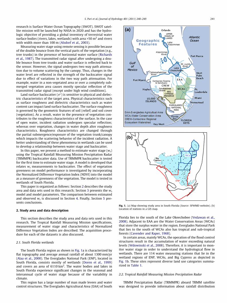
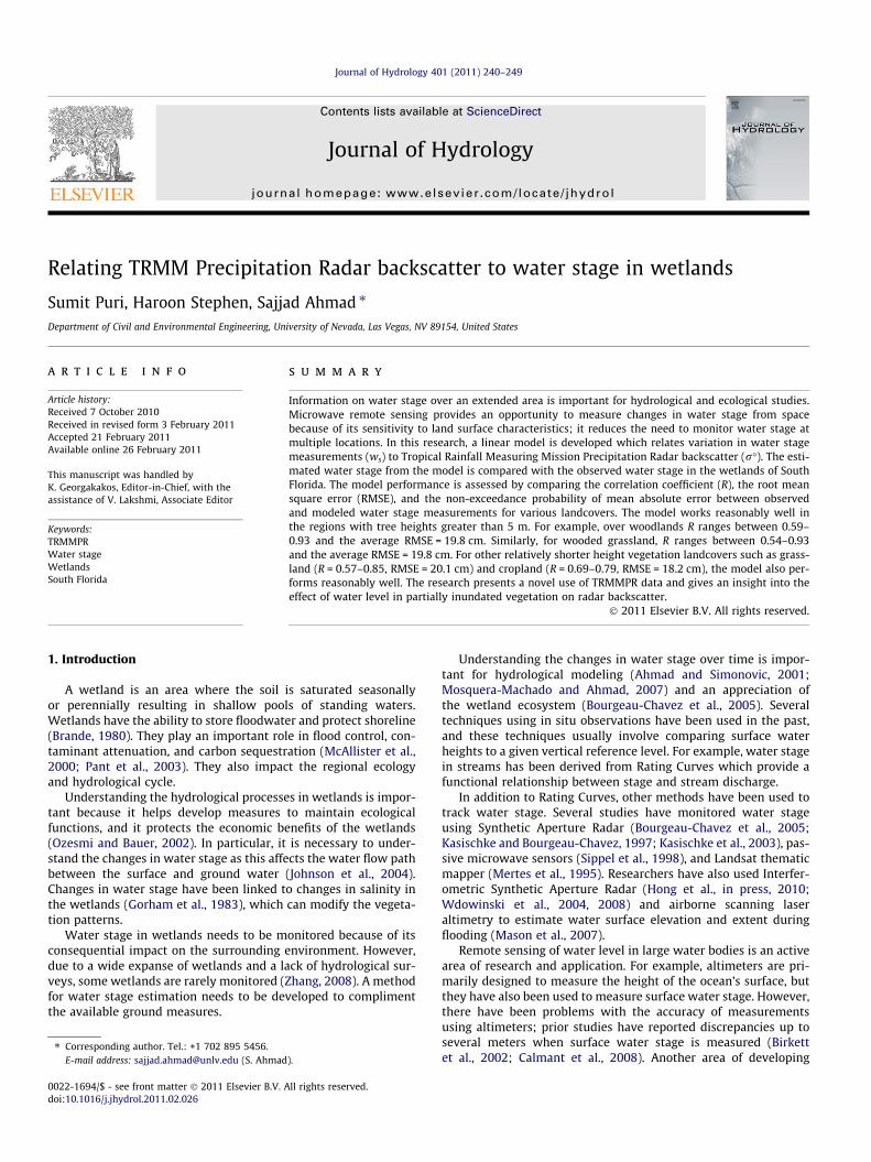
Fig. 1. (a) Map showing study area in South Florida (Source: SFWMD website). (b)Location of stations in a GIS map.

S. Puri et al. / Journal of Hydrology 401 (2011) 240–249 241

research is Surface Water Ocean Topography (SWOT). SWOT satel-lite mission will be launched by NASA in 2020 and has the hydro-logic objective of providing a global inventory of terrestrial watersurface bodies (rivers, lakes, wetlands) with area >50 m2 and riverswith width more than 100 m (Alsdorf et al., 2003).

Measuring water stage using remote sensing is possible becauseof the double bounce from the vertical parts of the vegetation (e.g.,tree trunks) in the presence of horizontal water surface (Richardset al., 1987). The transmitted radar signal after undergoing a dou-ble bounce from tree trunks and water surface is reflected back tothe sensor. However, the signal undergoes two way path attenua-tion due to volume scattering by the canopy. Thus, changes in thewater level are reflected in the strength of the backscatter signaldue to effect of variations in the two way path attenuation. Forexample, water in a non-vegetated area or over a completely sub-merged vegetation area causes mostly specular reflection of thetransmitted radar signal (except under high wind conditions).

Land surface backscatter (r�) is sensitive to physical and dielec-tric characteristics of the target area. Physical characteristics suchas surface roughness and dielectric characteristics such as watercontent can impact land surface backscatter. The surface roughnessis governed by the geometric features of soil (relief) and soil cover(vegetation). As a result, water in the presence of vegetation con-tributes to the roughness characteristics of the surface. In the caseof open water, incident radiation undergoes specular reflection;whereas over vegetation, changes in water depth alter roughnesscharacteristics. Roughness characteristics are changed throughthe partial submergence/exposure of the vegetation trunk/canopywhich impacts the scattering behavior of the incident radiation. Abetter understanding of these phenomena in wetlands can be usedto develop a relationship between water stage and backscatter.

In this paper, we present a method to estimate water stage (ws)using the Tropical Rainfall Measuring Mission Precipitation Radar(TRMMPR) backscatter data. Use of TRMMPR backscatter is testedfor the first time to estimate water stage. A model is developed thatrelates ws measurements to backscatter. The effect of vegetationgreenness on model performance is investigated by incorporatingthe Normalized Difference Vegetation Index (NDVI) into the modelas a measure of greenness of the vegetation. The model is tested inwetlands of South Florida.

This paper is organized as follows: Section 2 describes the studyarea and data sets used in this research; Section 3 presents the ws

model and model parameters. The comparison between estimatedand observed ws is discussed in Section 4. Finally, Section 5 pre-sents conclusions.

2. Study area and data description

This section describes the study area and data sets used in thisresearch. The Tropical Rainfall Measuring Mission specifications,measurement of water stage and characteristics of NormalizedDifference Vegetation Index are described. The acquisition proce-dure for each of the datasets is also discussed.

2.1. South Florida wetlands

The South Florida region as shown in Fig. 1a is characterized byflat topography and average annual rainfall of about 1300 mm/yr(Alaa et al., 2000). The Everglades National Park (ENP), located inSouth Florida, consists mostly of wetlands (Doren et al., 1999)and covers an area of 6110 km2. The water bodies and lakes inSouth Florida experience significant changes in the seasonal andinterannual cycle of water stage because of the variability inclimate.

This region has a large number of man made levees and watercontrol structures. The Everglades Agricultural Area (EAA) of South

Florida lies to the south of the Lake Okeechobee (Vedawan et al.,2008). Adjacent to EAA are the Water Conservation Areas (WCAs)that store the surplus water in the region. Everglades National Parkthat lies to the south of WCAs also has tropical and sub-tropicalforests (Cavender and Raper, 1968).

In certain areas, mainly WCAs, the operation of the flood controlstructures result in the accumulation of water exceeding naturallevels (Wdowinski et al., 2008). Therefore, it is important to mon-itor water stage in order to understand the hydrological flow inwetlands. There are 114 water measuring stations that lie in thewetland regions of ENP, WCAs, and Big Cypress as depicted inFig. 1b. These sites represent diverse land use categories summa-rized in Table 1.

2.2. Tropical Rainfall Measuring Mission Precipitation Radar

TRMM Precipitation Radar (TRMMPR) aboard TRMM satellitewas designed to provide information about rainfall distribution

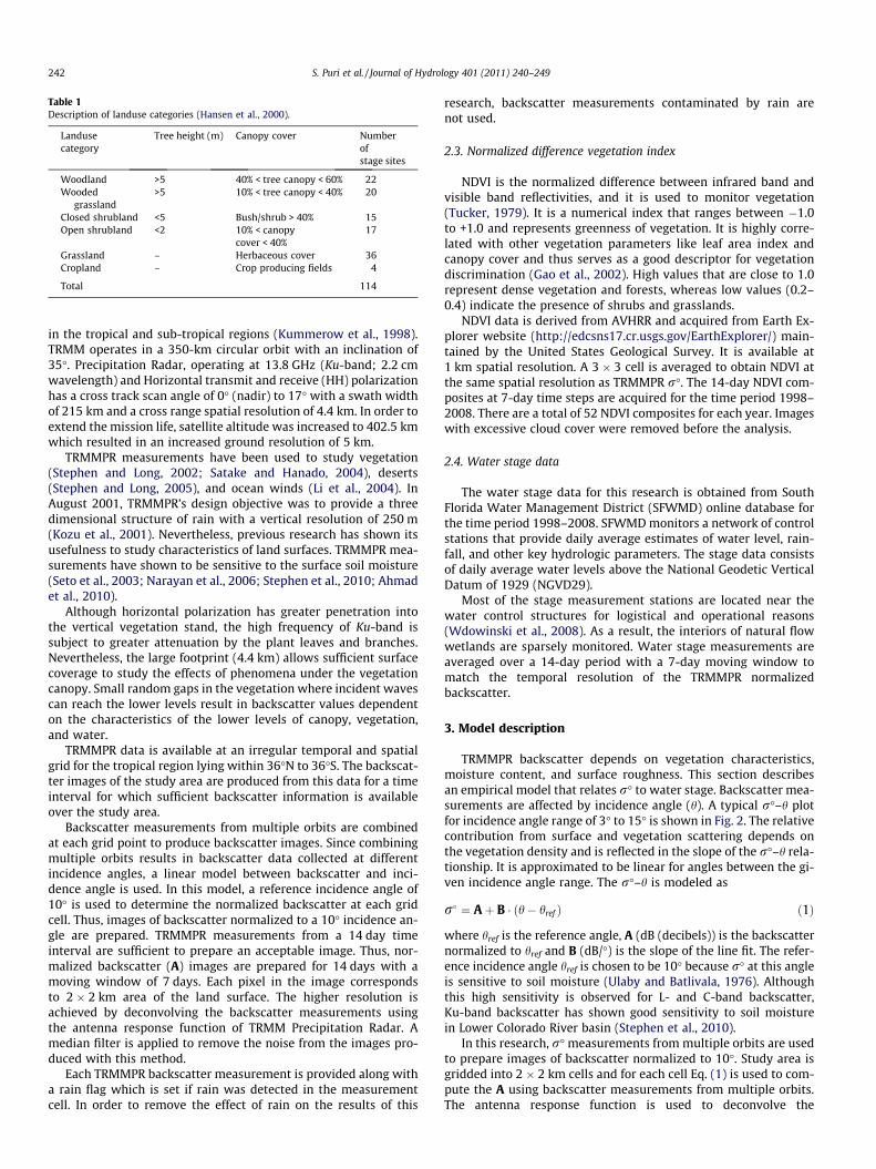
Table 1Description of landuse categories (Hansen et al., 2000).

Landusecategory

Tree height (m) Canopy cover Numberofstage sites

Woodland >5 40% < tree canopy < 60% 22Wooded

grassland>5 10% < tree canopy < 40% 20

Closed shrubland <5 Bush/shrub > 40% 15Open shrubland <2 10% < canopy

cover < 40%17

Grassland – Herbaceous cover 36Cropland – Crop producing fields 4

Total 114

242 S. Puri et al. / Journal of Hydrology 401 (2011) 240–249

in the tropical and sub-tropical regions (Kummerow et al., 1998).TRMM operates in a 350-km circular orbit with an inclination of35�. Precipitation Radar, operating at 13.8 GHz (Ku-band; 2.2 cmwavelength) and Horizontal transmit and receive (HH) polarizationhas a cross track scan angle of 0� (nadir) to 17� with a swath widthof 215 km and a cross range spatial resolution of 4.4 km. In order toextend the mission life, satellite altitude was increased to 402.5 kmwhich resulted in an increased ground resolution of 5 km.

TRMMPR measurements have been used to study vegetation(Stephen and Long, 2002; Satake and Hanado, 2004), deserts(Stephen and Long, 2005), and ocean winds (Li et al., 2004). InAugust 2001, TRMMPR’s design objective was to provide a threedimensional structure of rain with a vertical resolution of 250 m(Kozu et al., 2001). Nevertheless, previous research has shown itsusefulness to study characteristics of land surfaces. TRMMPR mea-surements have shown to be sensitive to the surface soil moisture(Seto et al., 2003; Narayan et al., 2006; Stephen et al., 2010; Ahmadet al., 2010).

Although horizontal polarization has greater penetration intothe vertical vegetation stand, the high frequency of Ku-band issubject to greater attenuation by the plant leaves and branches.Nevertheless, the large footprint (4.4 km) allows sufficient surfacecoverage to study the effects of phenomena under the vegetationcanopy. Small random gaps in the vegetation where incident wavescan reach the lower levels result in backscatter values dependenton the characteristics of the lower levels of canopy, vegetation,and water.

TRMMPR data is available at an irregular temporal and spatialgrid for the tropical region lying within 36�N to 36�S. The backscat-ter images of the study area are produced from this data for a timeinterval for which sufficient backscatter information is availableover the study area.

Backscatter measurements from multiple orbits are combinedat each grid point to produce backscatter images. Since combiningmultiple orbits results in backscatter data collected at differentincidence angles, a linear model between backscatter and inci-dence angle is used. In this model, a reference incidence angle of10� is used to determine the normalized backscatter at each gridcell. Thus, images of backscatter normalized to a 10� incidence an-gle are prepared. TRMMPR measurements from a 14 day timeinterval are sufficient to prepare an acceptable image. Thus, nor-malized backscatter (A) images are prepared for 14 days with amoving window of 7 days. Each pixel in the image correspondsto 2 � 2 km area of the land surface. The higher resolution isachieved by deconvolving the backscatter measurements usingthe antenna response function of TRMM Precipitation Radar. Amedian filter is applied to remove the noise from the images pro-duced with this method.

Each TRMMPR backscatter measurement is provided along witha rain flag which is set if rain was detected in the measurementcell. In order to remove the effect of rain on the results of this

research, backscatter measurements contaminated by rain arenot used.

2.3. Normalized difference vegetation index

NDVI is the normalized difference between infrared band andvisible band reflectivities, and it is used to monitor vegetation(Tucker, 1979). It is a numerical index that ranges between �1.0to +1.0 and represents greenness of vegetation. It is highly corre-lated with other vegetation parameters like leaf area index andcanopy cover and thus serves as a good descriptor for vegetationdiscrimination (Gao et al., 2002). High values that are close to 1.0represent dense vegetation and forests, whereas low values (0.2–0.4) indicate the presence of shrubs and grasslands.

NDVI data is derived from AVHRR and acquired from Earth Ex-plorer website (http://edcsns17.cr.usgs.gov/EarthExplorer/) main-tained by the United States Geological Survey. It is available at1 km spatial resolution. A 3 � 3 cell is averaged to obtain NDVI atthe same spatial resolution as TRMMPR r�. The 14-day NDVI com-posites at 7-day time steps are acquired for the time period 1998–2008. There are a total of 52 NDVI composites for each year. Imageswith excessive cloud cover were removed before the analysis.

2.4. Water stage data

The water stage data for this research is obtained from SouthFlorida Water Management District (SFWMD) online database forthe time period 1998–2008. SFWMD monitors a network of controlstations that provide daily average estimates of water level, rain-fall, and other key hydrologic parameters. The stage data consistsof daily average water levels above the National Geodetic VerticalDatum of 1929 (NGVD29).

Most of the stage measurement stations are located near thewater control structures for logistical and operational reasons(Wdowinski et al., 2008). As a result, the interiors of natural flowwetlands are sparsely monitored. Water stage measurements areaveraged over a 14-day period with a 7-day moving window tomatch the temporal resolution of the TRMMPR normalizedbackscatter.

3. Model description

TRMMPR backscatter depends on vegetation characteristics,moisture content, and surface roughness. This section describesan empirical model that relates r� to water stage. Backscatter mea-surements are affected by incidence angle (h). A typical r�–h plotfor incidence angle range of 3� to 15� is shown in Fig. 2. The relativecontribution from surface and vegetation scattering depends onthe vegetation density and is reflected in the slope of the r�–h rela-tionship. It is approximated to be linear for angles between the gi-ven incidence angle range. The r�–h is modeled as

r� ¼ Aþ B � ðh� href Þ ð1Þ

where href is the reference angle, A (dB (decibels)) is the backscatternormalized to href and B (dB/�) is the slope of the line fit. The refer-ence incidence angle href is chosen to be 10� because r� at this angleis sensitive to soil moisture (Ulaby and Batlivala, 1976). Althoughthis high sensitivity is observed for L- and C-band backscatter,Ku-band backscatter has shown good sensitivity to soil moisturein Lower Colorado River basin (Stephen et al., 2010).

In this research, r� measurements from multiple orbits are usedto prepare images of backscatter normalized to 10�. Study area isgridded into 2 � 2 km cells and for each cell Eq. (1) is used to com-pute the A using backscatter measurements from multiple orbits.The antenna response function is used to deconvolve the

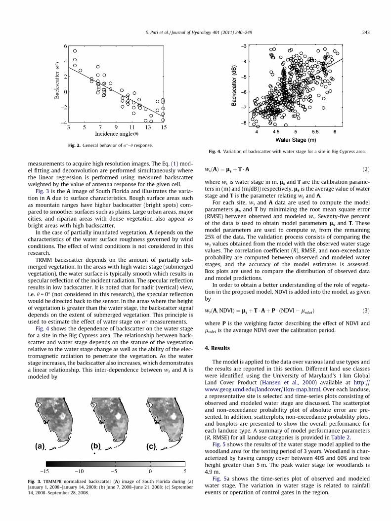
Fig. 2. General behavior of r�–h response.Fig. 4. Variation of backscatter with water stage for a site in Big Cypress area.

S. Puri et al. / Journal of Hydrology 401 (2011) 240–249 243

measurements to acquire high resolution images. The Eq. (1) mod-el fitting and deconvolution are performed simultaneously wherethe linear regression is performed using measured backscatterweighted by the value of antenna response for the given cell.

Fig. 3 is the A image of South Florida and illustrates the varia-tion in A due to surface characteristics. Rough surface areas suchas mountain ranges have higher backscatter (bright spots) com-pared to smoother surfaces such as plains. Large urban areas, majorcities, and riparian areas with dense vegetation also appear asbright areas with high backscatter.

In the case of partially inundated vegetation, A depends on thecharacteristics of the water surface roughness governed by windconditions. The effect of wind conditions is not considered in thisresearch.

TRMM backscatter depends on the amount of partially sub-merged vegetation. In the areas with high water stage (submergedvegetation), the water surface is typically smooth which results inspecular reflection of the incident radiation. The specular reflectionresults in low backscatter. It is noted that for nadir (vertical) view,i.e. h = 0� (not considered in this research), the specular reflectionwould be directed back to the sensor. In the areas where the heightof vegetation is greater than the water stage, the backscatter signaldepends on the extent of submerged vegetation. This principle isused to estimate the effect of water stage on r� measurements.

Fig. 4 shows the dependence of backscatter on the water stagefor a site in the Big Cypress area. The relationship between back-scatter and water stage depends on the stature of the vegetationrelative to the water stage change as well as the ability of the elec-tromagnetic radiation to penetrate the vegetation. As the waterstage increases, the backscatter also increases, which demonstratesa linear relationship. This inter-dependence between ws and A ismodeled by

Fig. 3. TRMMPR normalized backscatter (A) image of South Florida during (a)January 1, 2008–January 14, 2008; (b) June 7, 2008–June 21, 2008; (c) September14, 2008–September 28, 2008.

wsðAÞ ¼ ls þ T � A ð2Þ

where ws is water stage in m. ls and T are the calibration parame-ters in (m) and (m/dB)) respectively. ls is the average value of waterstage and T is the parameter relating ws and A.

For each site, ws and A data are used to compute the modelparameters ls and T by minimizing the root mean square error(RMSE) between observed and modeled ws. Seventy-five percentof the data is used to obtain model parameters ls and T. Thesemodel parameters are used to compute ws from the remaining25% of the data. The validation process consists of comparing thews values obtained from the model with the observed water stagevalues. The correlation coefficient (R), RMSE, and non-exceedanceprobability are computed between observed and modeled waterstages, and the accuracy of the model estimates is assessed.Box plots are used to compare the distribution of observed dataand model predictions.

In order to obtain a better understanding of the role of vegeta-tion in the proposed model, NDVI is added into the model, as givenby

wsðA;NDVIÞ ¼ ls þ T � Aþ P � ðNDVI� lndviÞ ð3Þ

where P is the weighing factor describing the effect of NDVI andlndvi is the average NDVI over the calibration period.

4. Results

The model is applied to the data over various land use types andthe results are reported in this section. Different land use classeswere identified using the University of Maryland’s 1 km GlobalLand Cover Product (Hansen et al., 2000) available at http://www.geog.umd.edu/landcover/1km-map.html. Over each landuse,a representative site is selected and time-series plots consisting ofobserved and modeled water stage are discussed. The scatterplotand non-exceedance probability plot of absolute error are pre-sented. In addition, scatterplots, non-exceedance probability plots,and boxplots are presented to show the overall performance foreach landuse type. A summary of model performance parameters(R, RMSE) for all landuse categories is provided in Table 2.

Fig. 5 shows the results of the water stage model applied to thewoodland area for the testing period of 3 years. Woodland is char-acterized by having canopy cover between 40% and 60% and treeheight greater than 5 m. The peak water stage for woodlands is4.9 m.

Fig. 5a shows the time-series plot of observed and modeledwater stage. The variation in water stage is related to rainfallevents or operation of control gates in the region.

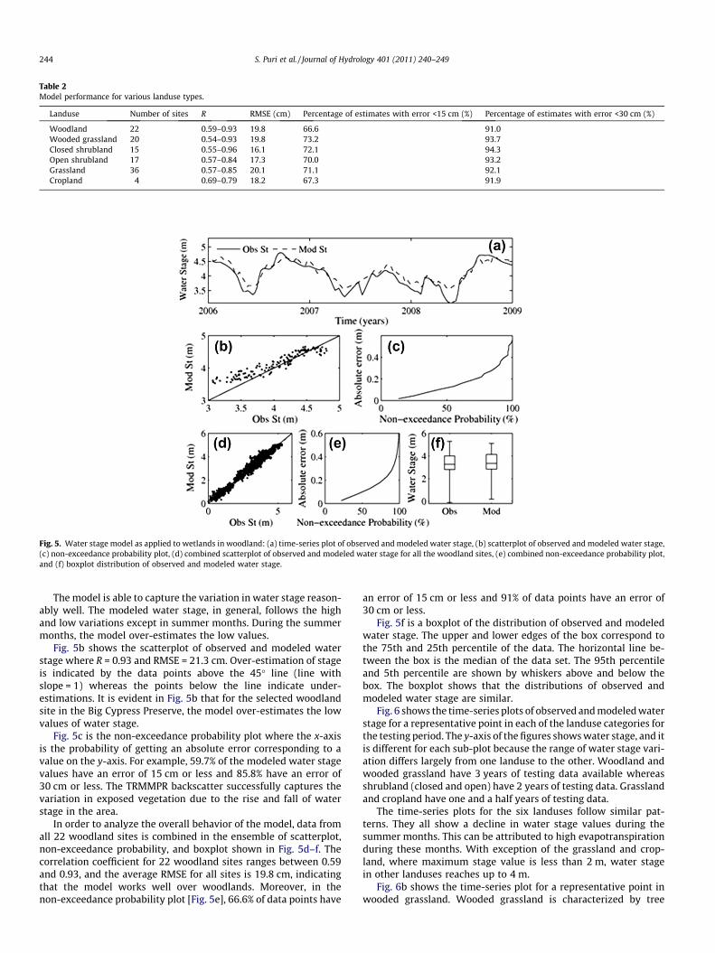
Table 2Model performance for various landuse types.

Landuse Number of sites R RMSE (cm) Percentage of estimates with error <15 cm (%) Percentage of estimates with error <30 cm (%)

Woodland 22 0.59–0.93 19.8 66.6 91.0Wooded grassland 20 0.54–0.93 19.8 73.2 93.7Closed shrubland 15 0.55–0.96 16.1 72.1 94.3Open shrubland 17 0.57–0.84 17.3 70.0 93.2Grassland 36 0.57–0.85 20.1 71.1 92.1Cropland 4 0.69–0.79 18.2 67.3 91.9

Fig. 5. Water stage model as applied to wetlands in woodland: (a) time-series plot of observed and modeled water stage, (b) scatterplot of observed and modeled water stage,(c) non-exceedance probability plot, (d) combined scatterplot of observed and modeled water stage for all the woodland sites, (e) combined non-exceedance probability plot,and (f) boxplot distribution of observed and modeled water stage.

244 S. Puri et al. / Journal of Hydrology 401 (2011) 240–249

The model is able to capture the variation in water stage reason-ably well. The modeled water stage, in general, follows the highand low variations except in summer months. During the summermonths, the model over-estimates the low values.

Fig. 5b shows the scatterplot of observed and modeled waterstage where R = 0.93 and RMSE = 21.3 cm. Over-estimation of stageis indicated by the data points above the 45� line (line withslope = 1) whereas the points below the line indicate under-estimations. It is evident in Fig. 5b that for the selected woodlandsite in the Big Cypress Preserve, the model over-estimates the lowvalues of water stage.

Fig. 5c is the non-exceedance probability plot where the x-axisis the probability of getting an absolute error corresponding to avalue on the y-axis. For example, 59.7% of the modeled water stagevalues have an error of 15 cm or less and 85.8% have an error of30 cm or less. The TRMMPR backscatter successfully captures thevariation in exposed vegetation due to the rise and fall of waterstage in the area.

In order to analyze the overall behavior of the model, data fromall 22 woodland sites is combined in the ensemble of scatterplot,non-exceedance probability, and boxplot shown in Fig. 5d–f. Thecorrelation coefficient for 22 woodland sites ranges between 0.59and 0.93, and the average RMSE for all sites is 19.8 cm, indicatingthat the model works well over woodlands. Moreover, in thenon-exceedance probability plot [Fig. 5e], 66.6% of data points have

an error of 15 cm or less and 91% of data points have an error of30 cm or less.

Fig. 5f is a boxplot of the distribution of observed and modeledwater stage. The upper and lower edges of the box correspond tothe 75th and 25th percentile of the data. The horizontal line be-tween the box is the median of the data set. The 95th percentileand 5th percentile are shown by whiskers above and below thebox. The boxplot shows that the distributions of observed andmodeled water stage are similar.

Fig. 6 shows the time-series plots of observed and modeled waterstage for a representative point in each of the landuse categories forthe testing period. The y-axis of the figures shows water stage, and itis different for each sub-plot because the range of water stage vari-ation differs largely from one landuse to the other. Woodland andwooded grassland have 3 years of testing data available whereasshrubland (closed and open) have 2 years of testing data. Grasslandand cropland have one and a half years of testing data.

The time-series plots for the six landuses follow similar pat-terns. They all show a decline in water stage values during thesummer months. This can be attributed to high evapotranspirationduring these months. With exception of the grassland and crop-land, where maximum stage value is less than 2 m, water stagein other landuses reaches up to 4 m.

Fig. 6b shows the time-series plot for a representative point inwooded grassland. Wooded grassland is characterized by tree

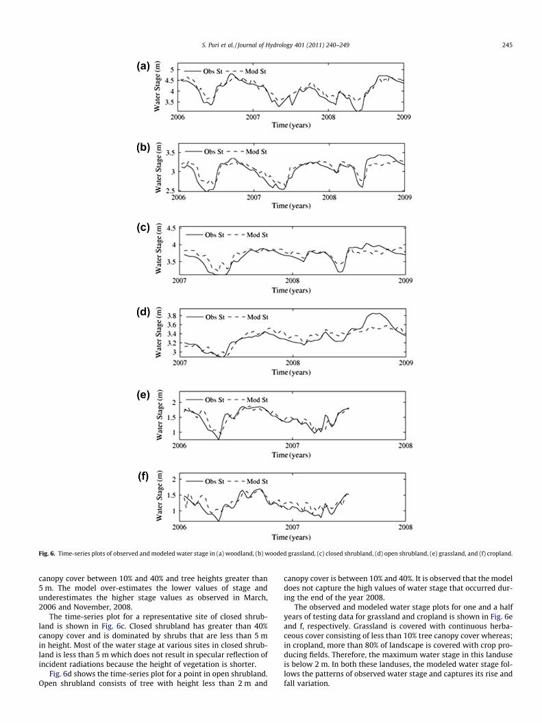
Fig. 6. Time-series plots of observed and modeled water stage in (a) woodland, (b) wooded grassland, (c) closed shrubland, (d) open shrubland, (e) grassland, and (f) cropland.

S. Puri et al. / Journal of Hydrology 401 (2011) 240–249 245

canopy cover between 10% and 40% and tree heights greater than5 m. The model over-estimates the lower values of stage andunderestimates the higher stage values as observed in March,2006 and November, 2008.

The time-series plot for a representative site of closed shrub-land is shown in Fig. 6c. Closed shrubland has greater than 40%canopy cover and is dominated by shrubs that are less than 5 min height. Most of the water stage at various sites in closed shrub-land is less than 5 m which does not result in specular reflection ofincident radiations because the height of vegetation is shorter.

Fig. 6d shows the time-series plot for a point in open shrubland.Open shrubland consists of tree with height less than 2 m and

canopy cover is between 10% and 40%. It is observed that the modeldoes not capture the high values of water stage that occurred dur-ing the end of the year 2008.

The observed and modeled water stage plots for one and a halfyears of testing data for grassland and cropland is shown in Fig. 6eand f, respectively. Grassland is covered with continuous herba-ceous cover consisting of less than 10% tree canopy cover whereas;in cropland, more than 80% of landscape is covered with crop pro-ducing fields. Therefore, the maximum water stage in this landuseis below 2 m. In both these landuses, the modeled water stage fol-lows the patterns of observed water stage and captures its rise andfall variation.

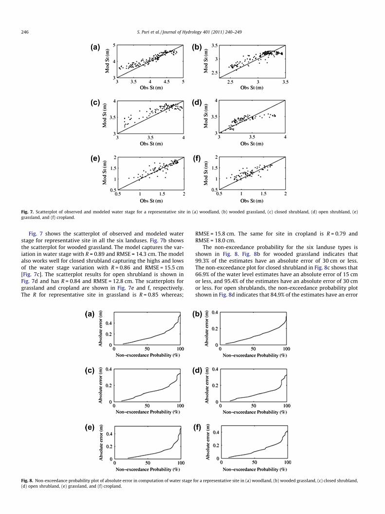
Fig. 7. Scatterplot of observed and modeled water stage for a representative site in (a) woodland, (b) wooded grassland, (c) closed shrubland, (d) open shrubland, (e)grassland, and (f) cropland.

246 S. Puri et al. / Journal of Hydrology 401 (2011) 240–249

Fig. 7 shows the scatterplot of observed and modeled waterstage for representative site in all the six landuses. Fig. 7b showsthe scatterplot for wooded grassland. The model captures the var-iation in water stage with R = 0.89 and RMSE = 14.3 cm. The modelalso works well for closed shrubland capturing the highs and lowsof the water stage variation with R = 0.86 and RMSE = 15.5 cm[Fig. 7c]. The scatterplot results for open shrubland is shown inFig. 7d and has R = 0.84 and RMSE = 12.8 cm. The scatterplots forgrassland and cropland are shown in Fig. 7e and f, respectively.The R for representative site in grassland is R = 0.85 whereas;

Fig. 8. Non-exceedance probability plot of absolute error in computation of water stage f(d) open shrubland, (e) grassland, and (f) cropland.

RMSE = 15.8 cm. The same for site in cropland is R = 0.79 andRMSE = 18.0 cm.

The non-exceedance probability for the six landuse types isshown in Fig. 8. Fig. 8b for wooded grassland indicates that99.3% of the estimates have an absolute error of 30 cm or less.The non-exceedance plot for closed shrubland in Fig. 8c shows that66.9% of the water level estimates have an absolute error of 15 cmor less, and 95.4% of the estimates have an absolute error of 30 cmor less. For open shrublands, the non-exceedance probability plotshown in Fig. 8d indicates that 84.9% of the estimates have an error

or a representative site in (a) woodland, (b) wooded grassland, (c) closed shrubland,

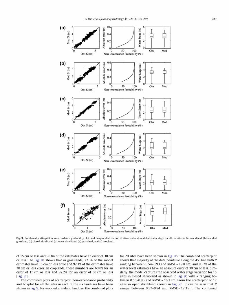
Fig. 9. Combined scatterplot, non-exceedance probability plot, and boxplot distribution of observed and modeled water stage for all the sites in (a) woodland, (b) woodedgrassland, (c) closed shrubland, (d) open shrubland, (e) grassland, and (f) cropland.

S. Puri et al. / Journal of Hydrology 401 (2011) 240–249 247

of 15 cm or less and 96.8% of the estimates have an error of 30 cmor less. The Fig. 8e shows that in grasslands, 77.3% of the modelestimates have 15 cm or less error and 92.1% of the estimates have30 cm or less error. In croplands, these numbers are 60.0% for anerror of 15 cm or less and 92.2% for an error of 30 cm or less[Fig. 8f].

The combined plots of scatterplot, non-exceedance probabilityand boxplot for all the sites in each of the six landuses have beenshown in Fig. 9. For wooded grassland landuse, the combined plots

for 20 sites have been shown in Fig. 9b. The combined scatterplotshows that majority of the data points lie along the 45� line with Rranging between 0.54–0.93 and RMSE = 19.8 cm; and 93.7% of thewater level estimates have an absolute error of 30 cm or less. Sim-ilarly, the model captures the observed water stage variation for 15sites in closed shrubland as shown in Fig. 9c with R ranging be-tween 0.55–0.96 and RMSE = 16.1 cm. From the scatterplot of 17sites in open shrubland shown in Fig. 9d, it can be seen that Rranges between 0.57–0.84 and RMSE = 17.3 cm. The combined

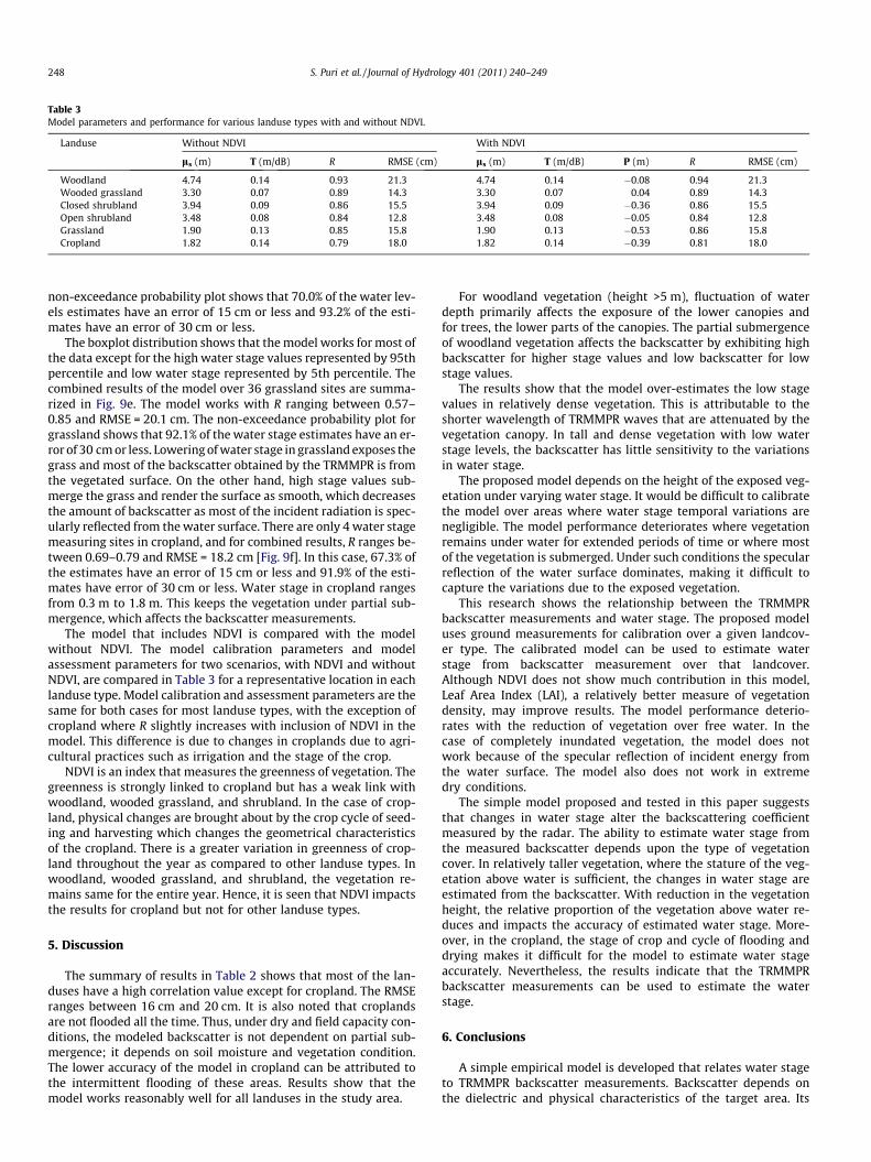
Table 3Model parameters and performance for various landuse types with and without NDVI.

Landuse Without NDVI With NDVI

ls (m) T (m/dB) R RMSE (cm) ls (m) T (m/dB) P (m) R RMSE (cm)

Woodland 4.74 0.14 0.93 21.3 4.74 0.14 �0.08 0.94 21.3Wooded grassland 3.30 0.07 0.89 14.3 3.30 0.07 0.04 0.89 14.3Closed shrubland 3.94 0.09 0.86 15.5 3.94 0.09 �0.36 0.86 15.5Open shrubland 3.48 0.08 0.84 12.8 3.48 0.08 �0.05 0.84 12.8Grassland 1.90 0.13 0.85 15.8 1.90 0.13 �0.53 0.86 15.8Cropland 1.82 0.14 0.79 18.0 1.82 0.14 �0.39 0.81 18.0

248 S. Puri et al. / Journal of Hydrology 401 (2011) 240–249

non-exceedance probability plot shows that 70.0% of the water lev-els estimates have an error of 15 cm or less and 93.2% of the esti-mates have an error of 30 cm or less.

The boxplot distribution shows that the model works for most ofthe data except for the high water stage values represented by 95thpercentile and low water stage represented by 5th percentile. Thecombined results of the model over 36 grassland sites are summa-rized in Fig. 9e. The model works with R ranging between 0.57–0.85 and RMSE = 20.1 cm. The non-exceedance probability plot forgrassland shows that 92.1% of the water stage estimates have an er-ror of 30 cm or less. Lowering of water stage in grassland exposes thegrass and most of the backscatter obtained by the TRMMPR is fromthe vegetated surface. On the other hand, high stage values sub-merge the grass and render the surface as smooth, which decreasesthe amount of backscatter as most of the incident radiation is spec-ularly reflected from the water surface. There are only 4 water stagemeasuring sites in cropland, and for combined results, R ranges be-tween 0.69–0.79 and RMSE = 18.2 cm [Fig. 9f]. In this case, 67.3% ofthe estimates have an error of 15 cm or less and 91.9% of the esti-mates have error of 30 cm or less. Water stage in cropland rangesfrom 0.3 m to 1.8 m. This keeps the vegetation under partial sub-mergence, which affects the backscatter measurements.

The model that includes NDVI is compared with the modelwithout NDVI. The model calibration parameters and modelassessment parameters for two scenarios, with NDVI and withoutNDVI, are compared in Table 3 for a representative location in eachlanduse type. Model calibration and assessment parameters are thesame for both cases for most landuse types, with the exception ofcropland where R slightly increases with inclusion of NDVI in themodel. This difference is due to changes in croplands due to agri-cultural practices such as irrigation and the stage of the crop.

NDVI is an index that measures the greenness of vegetation. Thegreenness is strongly linked to cropland but has a weak link withwoodland, wooded grassland, and shrubland. In the case of crop-land, physical changes are brought about by the crop cycle of seed-ing and harvesting which changes the geometrical characteristicsof the cropland. There is a greater variation in greenness of crop-land throughout the year as compared to other landuse types. Inwoodland, wooded grassland, and shrubland, the vegetation re-mains same for the entire year. Hence, it is seen that NDVI impactsthe results for cropland but not for other landuse types.

5. Discussion

The summary of results in Table 2 shows that most of the lan-duses have a high correlation value except for cropland. The RMSEranges between 16 cm and 20 cm. It is also noted that croplandsare not flooded all the time. Thus, under dry and field capacity con-ditions, the modeled backscatter is not dependent on partial sub-mergence; it depends on soil moisture and vegetation condition.The lower accuracy of the model in cropland can be attributed tothe intermittent flooding of these areas. Results show that themodel works reasonably well for all landuses in the study area.

For woodland vegetation (height >5 m), fluctuation of waterdepth primarily affects the exposure of the lower canopies andfor trees, the lower parts of the canopies. The partial submergenceof woodland vegetation affects the backscatter by exhibiting highbackscatter for higher stage values and low backscatter for lowstage values.

The results show that the model over-estimates the low stagevalues in relatively dense vegetation. This is attributable to theshorter wavelength of TRMMPR waves that are attenuated by thevegetation canopy. In tall and dense vegetation with low waterstage levels, the backscatter has little sensitivity to the variationsin water stage.

The proposed model depends on the height of the exposed veg-etation under varying water stage. It would be difficult to calibratethe model over areas where water stage temporal variations arenegligible. The model performance deteriorates where vegetationremains under water for extended periods of time or where mostof the vegetation is submerged. Under such conditions the specularreflection of the water surface dominates, making it difficult tocapture the variations due to the exposed vegetation.

This research shows the relationship between the TRMMPRbackscatter measurements and water stage. The proposed modeluses ground measurements for calibration over a given landcov-er type. The calibrated model can be used to estimate waterstage from backscatter measurement over that landcover.Although NDVI does not show much contribution in this model,Leaf Area Index (LAI), a relatively better measure of vegetationdensity, may improve results. The model performance deterio-rates with the reduction of vegetation over free water. In thecase of completely inundated vegetation, the model does notwork because of the specular reflection of incident energy fromthe water surface. The model also does not work in extremedry conditions.

The simple model proposed and tested in this paper suggeststhat changes in water stage alter the backscattering coefficientmeasured by the radar. The ability to estimate water stage fromthe measured backscatter depends upon the type of vegetationcover. In relatively taller vegetation, where the stature of the veg-etation above water is sufficient, the changes in water stage areestimated from the backscatter. With reduction in the vegetationheight, the relative proportion of the vegetation above water re-duces and impacts the accuracy of estimated water stage. More-over, in the cropland, the stage of crop and cycle of flooding anddrying makes it difficult for the model to estimate water stageaccurately. Nevertheless, the results indicate that the TRMMPRbackscatter measurements can be used to estimate the waterstage.

6. Conclusions

A simple empirical model is developed that relates water stageto TRMMPR backscatter measurements. Backscatter depends onthe dielectric and physical characteristics of the target area. Its

S. Puri et al. / Journal of Hydrology 401 (2011) 240–249 249

dependence on the partial submergence of vegetation is used asthe basis of estimation of water stage from r� measurements.

The model works reasonably well over various landuse types inwetlands of South Florida. For various landuse types, the correla-tion between observed and modeled water stage ranges between0.54–0.96 and root mean square error ranges between 16.1 cmand 20.1 cm. A high correlation and low root mean square errorshows the strength of the model.

A model relating water stage to TRMMPR backscatter and NDVIis also developed and tested. NDVI accounts for vegetation green-ness, and it improves the model performance for cropland. Thishappens because NDVI has a strong link with the geometrical char-acteristics of the cropland and these characteristic change due tothe crop cycles and seasons of seeding and harvesting of crops.Over the other landuse types that are characterized by tall treesand shrubs, inclusion of NDVI in the model does not improve theresults. This occurs because there is not much variation in vegeta-tion growth from one season to the other. This research provides amethod to compliment the ground measurements of water stageusing spaceborne backscatter measurements. It provides a noveluse of TRMMPR data and gives an insight into the effect of waterlevel in partially inundated vegetation on radar backscatter.

Acknowledgements

The funding for this work was provided by National Oceanicand Atmospheric Administration’s Social Application and ResearchProgram (NOAA-SARP) Award NA070AR4310324.

References

Ahmad, S., Simonovic, S.P., 2001. Integration of heuristic knowledge with analyticaltools for selection of flood control measures. Canadian Journal of CivilEngineering 28 (2), 208–221.

Ahmad, S., Kalra, A., Stephen, H., 2010. Estimating soil moisture using remotesensing data: a machine learning approach. Advances in Water Resources 33(1), 69–80.

Alaa, A., Abtew, W., Horn, S.V., Khanal, N., 2000. Temporal and spatialcharacterization of rainfall over central and south Florida. Journal of theAmerican Water Resources Association 36 (4), 833–848.

Alsdorf, D., Lettenmaier, D., Vörösmarty, C., The NASA Surface Water WorkingGroup, 2003. The need for global, satellite-based observations of terrestrialsurface waters. EOS Transactions of AGU 84 (269), 275–276.

Birkett, C.M., Mertes, L.A.K., Dunne, T., Costa, M., Jasinski, J., 2002. Altimetric remotesensing of the Amazon: application of satellite radar altimetry. Journal ofGeophysical Research 107 (D20), 8059. doi:10.1029/2001JD000609.

Bourgeau-Chavez, L.L., Smith, K.B., Brunzell, S.M., Kasischke, E.S., Romanowicz, E.A.,Richardson, C.J., 2005. Remote monitoring of regional inundation patterns andhydroperiod in the greater everglades using synthetic aperture radar. Wetlands25 (1), 176–191.

Brande, J., 1980. Worthless, valuable, or what – an appraisal of wetlands. Journal ofSoil and Water Conservation 35 (1), 12–16.

Calmant, S., Seyler, F., Cretaux, J.F., 2008. Monitoring continental surface water bysatellite altimetry. Survey of Geophysics 29, 247–269. doi:10.1007/s10712-008-9051-1.

Cavender, J.C., Raper, K.B., 1968. The occurrence and distribution of Acrasieae inforests of subtropical and tropical America. American Journal of Botany 55 (4),504–513.

Doren, R.F., Rutchey, K., Welch, R., 1999. The Everglades: a perspective on therequirements and applications for vegetation map and database products.Photogrammetric Engineering and Remote Sensing 65 (2), 155–161.

Gao, F., Jin, Y.F., Li, X.W., Schaaf, C.B., Strahler, A.H., 2002. Bidirectional NDVI andatmospherically resistant BRDF inversion for vegetation canopy. IEEETransactions on Geoscience and Remote Sensing 40 (6), 1269–1278.

Gorham, E., Dean, W.E., Sanger, J.E., 1983. The chemical-composition of lakes in thenorth-central United-States. Limnology and Oceanography 28 (2), 287–301.

Hansen, M.C., DeFries, R.S., Townshend, J.R.G., Sohlberg, R., 2000. Global land coverclassification at 1 km spatial resolution using a classification tree approach.International Journal of Remote Sensing 21, 1331–1364.

Hong, S.H., Wdowinski, S., Kim, S.W., 2010. Evaluation of TerraSAR-X observationsfor wetland InSAR application. IEEE Geosciences and Remote Sensing 48, 864–873.

Hong, S.H., Wdowinski, S., Kim, S.W., in press. Space-based multi-temporalmonitoring of wetland water levels: case study of WCA1 in the Everglade,Remote Sensing for Environment.

Johnson, W.C., Boettcher, S.E., Poiani, K.A., Guntenspergen, G., 2004. Influence ofweather extremes on the water levels of glaciated prairie wetlands. Wetlands24 (2), 385–398.

Kasischke, E.S., Bourgeau-Chavez, L.L., 1997. Monitoring south florida wetlandsusing ERS-1 SAR imagery. Photogrammetric Engineering and Remote Sensing63 (3), 281–291.

Kasischke, E.S., Smith, K.B., Bourgeau-Chavez, L.L., Romanowicz, E.A., Brunzell, S.,Richardson, C.J., 2003. Effects of seasonal hydrologic patterns in south Floridawetlands on radar backscatter measured from ERS-2 SAR imagery. RemoteSensing of Environment 88 (4), 423–441.

Kozu, T., Kawanishi, T., Kuroiwa, H., Kojima, M., Oikawa, K., Kumagai, H., et al., 2001.Development of precipitation radar onboard the tropical rainfall measuringmission (TRMM) satellite. IEEE Transactions on Geoscience and Remote Sensing39 (1), 102–116.

Kummerow, C., Barnes, W., Kozu, T., Shiue, J., Simpson, J., 1998. The tropical rainfallmeasuring mission (TRMM) sensor package. Journal of Atmospheric andOceanic Technology 15 (3), 809–817.

Li, L., Im, E., Connor, L.N., Chang, P.S., 2004. Retrieving ocean surface wind speedfrom the TRMM precipitation radar. IEEE Transactions on Geoscience andRemote Sensing 42 (6), 1271–1282.

Mason, D.C., Horritt, M.S., Dall’ Amico, J.T., Scott, T.R., Bates, P.D., 2007. Improvingriver flood extent delineation from synthetic aperture radar using airborne laseraltimetry. IEEE Transactions on Geoscience and Remote Sensing 45 (12), 3932–3943.

McAllister, L.S., Peniston, B.E., Leibowitz, S.G., Abbruzzese, B., Hyman, J.B., 2000. Asynoptic assessment for prioritizing wetland restoration efforts to optimizeflood attenuation. Wetlands 20 (1), 70–83.

Mertes, L.A.K., Daniel, D.L., Melack, J.M., Nelson, B., Martinelli, L.A., Forsberg, B.R.,1995. Spatial patterns of hydrology, geomorphology, and vegetation on thefloodplain of the Amazon river in Brazil from a remote sensing perspective.Geomorphology 13 (1–4), 215–232.

Mosquera-Machado, S.C., Ahmad, S., 2007. Flood hazard assessment of Atrato riverin Colombia. Water Resources Management 21, 591–609.

Narayan, U., Lakshmi, V., Jackson, T., 2006. A simple algorithm for spatialdisaggregation of radiometer derived soil moisture using higher resolutionradar observations. IEEE Transactions on Geoscience and Remote Sensing 44 (6),1545–1554.

Ozesmi, S.L., Bauer, M.E., 2002. Satellite remote sensing of wetlands. WetlandsEcology and Management 10 (5), 381–402.

Pant, H.K., Rechcigl, J.E., Adjei, M.B., 2003. Carbon sequestration in wetlands:concept and estimation. Journal of Food Agriculture and Environment 1 (2),308–313.

Richards, J.A., Woodgate, P.W., Skidmore, A.K., 1987. An explanation of enhancedradar backscattering from flooded forests. International Journal of RemoteSensing 8 (7), 1093–1100.

Satake, M., Hanado, H., 2004. Diurnal change of Amazon rain forest – observed byKu-band spaceborne radar. IEEE Transactions on Geoscience and RemoteSensing 42 (6), 1127–1134.

Seto, S., Oki, T., Musiake, K., 2003. Surface soil moisture estimation by TRMM/PR andTMI. In: Proceedings of International Geoscience and Remote SensingSymposium, vol. III, pp. 1960–1962.

Sippel, S.J., Hamilton, S.K., Melack, J.M., Novo, E.M.M., 1998. Passive microwaveobservations of inundation area and the area/stage relation in the Amazon Riverfloodplain. International Journal of Remote Sensing 19 (16), 3055–3074.

Stephen, H., Long, D.G., 2002. Multi-spectral analysis of the Amazon basin usingSeawinds, ERS, NASA, Seasat Scatterometer, TRMM-PR and SSM/I. In:Proceedings of International Geoscience and Remote Sensing Symposium, vol.5, Toronto, Canada, pp. 2808–2810.

Stephen, H., Long, D.G., 2005. Microwave backscatter modeling of erg surfaces in theSahara desert. IEEE Transactions on Geoscience and Remote Sensing 43 (2),238–247.

Stephen, H., Ahmad, S., Piechota, T.C., Tang, C., 2010. Relating surface backscatterresponse from TRMM precipitation radar to soil moisture: results over a semi-arid region. Hydrology and Earth System Sciences 14, 193–204.

Tucker, C.J., 1979. Red and photographic infrared linear combinations formonitoring vegetation. Remote Sensing of Environment 8 (2), 127–150.

Ulaby, F.T., Batlivala, P.P., 1976. Optimum radar parameters for mapping soil-moisture. IEEE Transactions on Geosciences and Remote Sensing 14 (2), 81–93.

Vedwan, N., Ahmad, S., Miralles-Wilhelm, F., Broad, K., Letson, D., Podesta, G., 2008.Institutional evolution in Lake Okeechobee Management in Florida:characteristics, impacts, and limitations. Water Resources Management 22,699–718.

Wdowinski, S., Amelung, F., Miralles-Wilhelm, F., Dixon, T., Carande, R., 2004.Space-based measurements of sheet-flow characteristics in the Evergladeswetland, Florida. Geophysical Research Letters 31, L15503.

Wdowinski, S., Kim, S.W., Amelung, F., Dixon, T.H., Miralles-Wilhelm, F., Sonenshein,R., 2008. Space-based detection of wetlands’ surface water level changes fromL-band SAR interferometry. Remote Sensing of Environment 112 (3), 681–696.

Zhang, B., 2008. Data Mining, GIS and Remote Sensing: Application in WetlandHydrological Investigation. Ohio State University, Ohio.