MARINE ECOLOGY PROGRESS SERIESMar Ecol Prog Ser

Vol. 471: 73–85, 2012doi: 10.3354/meps10036

Published December 19

INTRODUCTION

Blooms of jellyfish, often referring to pelagiccnidarians and ctenophores, have received increasedattention in recent years. Although disputed (Condonet al. 2012), there appears to be a trend towards morefrequent blooms, higher abundances, and wider geo-graphical distributions (Richardson et al. 2009, Brotzet al. 2012, Purcell 2012). Jellyfish mass occurrenceand apparent shifts from fish- to jellyfish-dominatedsystems have been linked to numerous factors suchas fisheries (Brodeur et al. 2002, Lynam et al. 2006,Daskalov et al. 2007), aquaculture (Lo et al. 2008),eutrophication (Parsons & Lalli 2002, Purcell et al.2007), hypoxia (Decker et al. 2004, Thuesen et al.2005), and water clarity (Aksnes 2007, Sørnes et al.2007). Furthermore, increased jellyfish abundances

have been linked to climate change, including tem-perature increase (Purcell et al. 2007, Lynam et al.2011), enhanced stratification (Richardson et al. 2009),and decreased pH (Richardson & Gibbons 2008).Finally, translocations of species, sometimes referredto as invasions of alien species, have also been seenas contributors to jellyfish blooms (Graham & Bayha2007).

The fact that jellyfish blooms have been linked tomany factors is not surprising since cnidarians andctenophores are diverse species groups with a vari-ety of life histories and environmental responses.Thus case-specific analyses and models (e.g. Sørneset al. 2007, Oguz et al. 2008, Dupont & Aksnes 2010,Ruiz et al. 2012) are undoubtedly needed to accountaccurately for observed phenomena. Nevertheless,we present an idealized analysis of the competitive

© Inter-Research 2012 · www.int-res.com*Corresponding author. Email: dag.aksnes@bio.uib.no

Relationship between fish and jellyfish as a functionof eutrophication and water clarity

Matilda Haraldsson1, Kajsa Tönnesson1, Peter Tiselius1, Tron Frede Thingstad2, Dag L. Aksnes2,*

1Department of Biological and Environmental Sciences, University of Gothenburg, Sweden2Department of Biology, University of Bergen, 5020 Bergen, Norway

ABSTRACT: There is a concern that blooms of cnidarians and ctenophores, often referred to as jel-lyfish, are increasing in frequency and intensity worldwide and that there is a shift from fish- tojellyfish-dominated systems. We present an idealized analysis of the competitive relationshipbetween zooplanktivorous jellyfish that is based on a generic model, termed ‘Killing the Winner’(KtW), for the coexistence of 2 groups utilizing the same resource. Tactile predation by jellyfishmakes them less dependent on water optics than fish using vision, and we modified the KtWmodel to account for this particular trait difference. Expectations of the model are illustrated byuse of observations from the Baltic Sea. The model predicts a general succession on how mass ofthe system distributes when going from an oligotrophic to a eutrophic system. Initially the mass ofthe system accumulates at the level of the common resource (zooplankton) and planktivorous fish(sprat/herring). At one point, with increased eutrophication, mass starts to accumulate at the levelof the top predator (cod) and at a later point, at the level of the jellyfish. For those organisms utilizing vision (fishes) an optimal degree of eutrophication and water clarity is predicted due to a2-sided effect of eutrophication.

KEY WORDS: Jellyfish · Fish · Competition · Killing the winner · Eutrophication · Water clarity

Resale or republication not permitted without written consent of the publisher

OPENPEN ACCESSCCESS

Mar Ecol Prog Ser 471: 73–85, 2012

relationship between fish and jellyfish that mightapply to certain circumstances. We start out with ageneric model of coexistence between 2 groupsof organisms that compete for the same resource(Fig. 1). This generic model, which is denoted ‘Killingthe Winner’ (KtW; Thingstad et al. 2010), containsa structure wherein a competition specialist is inplay with a predator while the other competitor, thedefense specialist, is not (Fig. 1). The equilibriumsolution of the KtW provides general predictions onhow the system responds to changes in the total massof limiting nutrients of the system, i.e. the degree ofeutrophication (Thingstad et al. 2010). Most KtWapplications have been on microbial systems (Winteret al. 2010) that are stimulated by increased nutrient

availability. Important aspects of the habitat of manyfishes, such as water clarity and visibility (Eggers1977, Lester et al. 2004, Aksnes 2007), however, tendto deteriorate at high degrees of eutrophication, andwe modified the model to account for such habitatdeterioration. We apply data from the Baltic Sea toillustrate KtW predictions on how eutrophication andwater clarity affects the competitive relationshipbetween fish and jellyfish. We do not consider thisapplication as a definitive test or validation (sensuLoehle 1983) of the model, but rather use the trans-parency and analytical tractability offered by theKtW simplification to gain general insights in jellyfishsystems that might comply with the assumptions ofthe KtW structure.

MATERIALS AND METHODS

Baltic Sea

The Baltic Sea, which we have used to estimatecoefficients of the model and to illustrate KtW pre -dictions, is a complex ecosystem that has experi-enced extensive changes during the last century.These changes involve eutrophication, reduced water clarity, and increased fishery, among other factors(Table 1). Nutrient inputs have increased (Struck etal. 2000, Savchuk et al. 2008), and the Baltic Sea hasturned from an oligotrophic to a eutrophic state(Meier et al. 2011). A low fish biomass during the firstpart of the 1900s has been indicated due to a lowerproductivity prior to eutrophication (Thurow 1997).The increased primary production has caused hyp -oxia (Diaz & Rosenberg 2008, Savchuk et al. 2008)

74

Fig. 1. Two generic principles of coexistence. (A) Coexis-tence is possible due to specialization for different sub-strates. (B) The same limiting resource is shared, but a selec-tive loss mechanism prevents the competition specialist fromsequestering all of the limiting resource, leaving a niche for

the defense specialist (after Thingstad et al. 2010)

Environmental Change Time period Sourcevariable

Eutrophication Increase 1850−2000 Struck et al. (2000)

Phytoplankton Increase (doubling 1905/06, 1912/13 Wasmund et al. (2008) over the century) 1949/50, and 2001−03

Hypoxia Increase 1960s Diaz & Rosenberg (2008)

Water clarity Reduced 0.05 m yr−1 1919−39,1969−91 Sanden & Håkansson (1996)

Pollutants Increase 1960s Elmgren (2001)

SST Increase 1870−2003 Mackenzie & Schiedek (2007) Increase 1900−2000 Fonselius & Valderrama (2003) 1.35°C increase 1982−2006 Belkin (2009)

Non-indigenous Tripled 1900−2000 Leppäkoski et al. (2002)species

Table 1. Some major environmental changes in the Baltic Sea during the last century. SST: sea surface temperature

Haraldsson et al.: Modeling fish and jellyfish relationships 75

and has reduced the water clarity (Sanden & Hå -kansson 1996, Fleming-Lehtinen & Laamanen 2012).Despite efforts to reduce nutrient inputs, eutrophica-tion symptoms persist (Backer & Leppanen 2008,Andersen et al. 2011) and water clarity remains low(Fleming-Lehtinen & Laamanen 2012). Over the last100 yr, phytoplankton biomass has doubled (Was-mund et al. 2008), phytoplankton composition haschanged (Was mund et al. 2008, Olli et al. 2011), andcyanobacterial blooms have been more frequent(Finni et al. 2001).

The commercial fishery in the Baltic Sea, domi-nated by cod, sprat, and herring, also increased dur-ing the 1900s (Mackenzie et al. 2007). The maximumcod biomass was reported for the early 1980s (Alheitet al. 2005). While fishing pressure increased duringthe mid-20th century (Mackenzie et al. 2007), the codbiomass decreased 10-fold by the end of the 1980s,shifting the Baltic from a cod-dominated to a sprat-dominated system (Casini et al. 2009).

The recent appearance of Mnemiopsis leidyi in theNorth Sea (Faasse & Bayha 2006), Kattegat area(Tendal et al. 2007), as well as in the Baltic Sea(Javidpour et al. 2006) has raised concerns about anincreased likelihood for future gelatinous massoccurrences. Aurelia aurita is presently the dominantjellyfish of the Baltic Sea (Möller 1980, Barz & Hirche2005, Haraldsson & Hansson 2011), which corre-sponds to the Black Sea situation before the M. leidyimass occurrences in the 1980s (Weisse & Gomoiu2000 and references therein). Cyanea capillata is thesecond-most abundant jellyfish in the Baltic, al -though 1 order of magnitude lower than A. aurita.

KtW model for the jellyfish−fish system

We consider a KtW structure (Figs. 1 & 2) wherezooplanktivorous jellyfish (J ) and fish (F) share acommon zooplankton (Z) resource, and where thezooplanktivorous fish are exposed to a top predator(C). This structure frames the zooplanktivorous jelly-fish and fish as the defense and the competition spe-cialist, respectively. We use Baltic Sea observationson Aurelia aurita and Cyanea capillata (Table 2) torepresent the jellyfish biomass and sprat togetherwith herring (Table 2) to show the biomass of thecompetitor. Cod is a predator of sprat and herring(Sparholt 1994, Casini et al. 2008) and is given therole as the top predator (Fig. 2, Table 2).

In KtW theory, which has primarily been applied tomicrobial systems (Winter et al. 2010), a quantity thatcorresponds to the total amount of a limiting nutrient

(also including the mass of the organisms), such asphosphorus, represents the degree of eutrophicationof the system (Thingstad et al. 2010). In our higher-trophy system, we use carbon (C), rather than a min-eral nutrient, as currency, and we will assume thatthe biomass of our idealized system is constrained bythe mass flowing through the zooplankton (PZ, g Cyr−1). In the Baltic Sea application, we let this massreflect the primary production, PP, according to PZ =TZPP where TZ corresponds to the transfer efficiencybetween primary and secondary production. Both PZ

and PP will be used as indices of the degree ofeutrophication.

According to Fig. 2, we specify the equations:

(1a)

(1b)

(1c)

(1d)

dZdt

P a Z F a Z JZ F J= − −

dJdt

Y a ZJ JJ j j= − δ

dFdt

Y a Z F a C F FF F C F= − − δ

dCdt

Y a F C CC C C= − δ

Fig. 2. ‘Killing the Winner’ model for coexistence betweenjellyfish and zooplanktivorous fish (sprat and herring) in theBaltic Sea. Fishery mortality is included in the loss rates δC

and δF, while the degree of eutrophication of the system isrepresented by the amount of mass that enters the systemthrough zooplankton (see ‘Materials and methods’). a and Yrepresent the predation coefficients and the transfer effi-ciencies (yields) between 2 trophic levels, respectively; e.g.aC is the specific predation rate of cod (C ) on sprat and her-ring (F ) so that the product aCFC is the amount of sprat andherring that is removed by cod per unit time (see Eq. 1c). Inorder to convert this amount to cod biomass, a yield, YC, is

applied (see Eq. 1d)

Mar Ecol Prog Ser 471: 73–85, 2012

where Z, J, F, and C are expressed in units of totalbiomass (g C) of the system. Solving for steady stateyields the equilibrium biomasses:

(2a)

(2b)

(2c)

(2d)

From Eq. (2b), we see that jellyfish existence (i.e.positive values of J*) requires that the degree ofeutrophication exceeds a threshold value:

(3)

For PZ less than this quantity, we eliminate jelly-fish, and the system of equations reduces to:

(4a)

(4b)

(4c)

which has the steady-state solution:

(5a)

(5b)

(5c)

From Eq. (5c), we see that cod existence (i.e. posi-tive values of C*) requires that PZ must exceed thethreshold:

(6)

For PZ less than this quantity, the system of equa-tions reduces to

(7a)

(7b)

which has the steady-state solution

(8a)

(8b)

C a Y Ya

PC F CC

CZ F*= −⎛

⎝⎞⎠

−1

δδ

PY Y aZ

F C

F C C

> δ δ

FY a

C

C C

*= δ

ZY a

aPC

C

C

FZ*=

δ

dZdt

P a Z FZ F= −

ZY a

J

J J

* = δ

JY

Pa

Y a aJ

JZ

F

C C JC*= −

δδ

FY a

C

C C

*= δ

C aYY

aaC

F

J

F

JJ F*= −⎛

⎝⎞⎠

−1 δ δ

Pa

Y Y a aZF

C J C JC J> δ δ

dZdt

P a Z FZ F= −

dFdt

Y a Z F a C F FF F C F= − − δ

dCdt

Y a F C CC C C= − δ

dFdt

Y a Z F FF F F= − δ

ZY a

F

F F

*= δ

FY

PF

FZ*=

δ

76

Group Biomass Landing Loss rate (δ) SourceWW ± SD Carbona WW yr−1 ± SD yr−1

Zooplankton (Z) 3.7 ± 1.0 0.220 Casini et al. (2008)

Jellyfish (J ) 60.8 ± 54.8 0.061 3.6 Barz & Hirche (2005),Haraldsson & Hansson (2011)

Sprat and herring (F ) 2.395 ± 0.227 0.240 0.493 ± 0.040 0.31Swedish Agency for Marine and

Cod (C ) 0.215 ± 0.053 0.022 0.087 ± 0.022 0.60 Water Management (2010)

Table 2. Biomasses (Mt) in the Baltic Sea used to estimate model coefficients. Means ± SD for the period 2000 to 2009 (exceptzooplankton: 2000 to 2006); jellyfish values are the average of sampling conducted in the Bornholm basin in September 2002and 2009 (20.5 and 99.5 Mt wet weight, WW, respectively). Loss rates for the fish groups represent catch or biomass, with anassumed natural mortality of 0.2 yr−1 for cod and 0.1 yr−1 for sprat and herring (the latter excludes cod predation, which is rep-resented in the model). Loss rate for jellyfish corresponds to a mortality of 1% d−1. We used the combined area of the BalticProper and the Gulf of Finland (258 310 km2) and assumed a vertical layer of 50 m in the conversion of zooplankton and jelly-fish to total biomasses from abundances specified per m3. aConversion from WW to carbon (C) with the factors 0.06 (C =0.5 DW, DW = 0.12 WW; Parsons et al. 1992) for zooplankton, 0.1 for fish (Arrhenius & Hansson 1993), and 0.001 (C = 0.05 DW,

DW = 0.02 WW; Schneider 1988) for jellyfish

⎫⎬⎭

Haraldsson et al.: Modeling fish and jellyfish relationships 77

Modified KtW model for the jellyfish−fish system

In the above model, increased eutrophicationimplies higher production and more zooplanktonavailable for fish and jellyfish, but essentiallyassumes that there are no negative effects fromeutrophication on the habitats of the organisms.While most jellyfish are tactile predators (Sørnes &Aksnes 2004, Acuña et al. 2011), many fishes arevisual predators that are affected by water clarity andvisibility (Eggers 1977, Lester et al. 2004, Aksnes2007), which tend to deteriorate with increasedeutrophication. Thus we now assume that the habi-tats of the fishes decline with increased eutrophica-tion, while the habitats of zooplankton and jellyfishare unaffected.

We express the habitat volumes of the 4 biomassgroups; Vx = A Hx where A (m2) corresponds to thecombined area of the Baltic Proper and the Gulf ofFinland (258 310 km2) and Hx (m) is the verticalextension of the habitat of biomass group x. The sys-tem of equations, with this explicit representation ofhabitat volumes, is given in Appendix 1.

We assume that the extensions of the vertical habi-tats, Hx, of the 2 fish groups are constrained by waterclarity according to (Aksnes 2007): Hx ∝ (c + K )–1,where c (m−1) is the beam (or image) attenuationcoefficient, and K (m−1) is the attenuation of down-welling irradiance. Both are key pro perties forunderwater vision (John sen 2012) and visual feeding(Eggers 1977, Aksnes & Utne 1997), where c deter-mines the maximal sighting distance of a visual pred-ator, and K de termines the light intensity at depth. Inpractice, different c and K values apply to differentwavelengths, but here we assume that the 2 quanti-ties are properties of all wave lengths relevant for theactual visual system.

Fortunately, the widely monitored Secchi diskdepth (S; m) does, like Hx, relate inversely to c and K,i.e. S ∝ (c + K )–1 (Preisendorfer 1986). Thus we have,Hx ∝ S, which means that changes in Secchidisk depth might serve as proxy for changesin the extension of the vertical vision basedhabitat of the fishes (Aksnes 2007), and wemake us of this proxy below.

Estimates of model coefficients

KtW model

Table 2 summarizes the values of the bio-masses and loss rates that we have used to

characterize the current Baltic Sea. Insertion of thesevalues into the steady-state equations (Eq. 2a−d) pro-vided estimates of the predation coefficients and thedegree of eutrophication (Table 3). The estimate of PZ

is 16.5 g C m−2 yr−1. According to Wasmund et al.(2001, their Table 5), the average primary production(PP) for the Baltic Proper and the Gulf of Finland cor-responds to 187 g C m−2 yr−1. These estimates indi-cate a transfer efficiency between primary and sec-ondary production, TZ = 16.5 / 187 = 0.09.

Modified KtW model

Here we need a relationship on how the verticalhabitat (Hx) is affected by eutrophication (i.e. by pri-mary production), and in order to establish this rela-tionship, some assumptions are required. First, weassume that a hypothetical water column, which isdevoid of phytoplankton (and consequently of pri-mary production), imposes no visual constraints onthe fishes. For this case, we consider the habitats ofzooplankton, jellies, and fishes to be equal (as alsoimplied in the basic KtW model). Second, as primaryproduction increases, we assume that the visual con-straints of the fishes also increase because water clarity deteriorates with increasing phytoplanktondensity.

Below we have approximated that if there were noprimary production (i.e. no chlorophyll), the BalticSea Secchi depth would have been twice (10 to 15 m)of what is observed, i.e. ~6 m (Fleming-Lehtinen &Laamanen 2012). To represent current primary pro-duction, we apply 187 g C m−2 yr−1 (Wasmund et al.2001), and interpolation then suggests a 2.7% de -crease in Secchi depth (S) for each 10 g C m−2 yr−1

rise in primary production. According to the proxy,Hx ∝ S, explained above, we also used this value torepresent the loss of fish habitat as a function of pri-mary production.

Symbol Estimate Unit

Mass entering zooplankton (Z ) PZ 4.3 Mt C yr−1

Expressed per surface area 16.5 g C m−2 yr−1

Predation coefficient of jellyfish (J ) aJ 163.6 (Mt C)−1 yr−1

sprat and herring (F ) aF 39.1 (Mt C)−1 yr−1

cod (C ) aC 25.0 (Mt C)−1 yr−1

Table 3. Predation coefficients (a in Fig. 2) of the basic ‘Killing the Win-ner’ model. These estimates were obtained by solving for steady state(Eq. 2) by insertion of the total biomasses and the loss rate estimates

in Table 2 and assuming all yields (Y ’s) equal to 0.1

Mar Ecol Prog Ser 471: 73–85, 2012

Insertion of the values of the biomasses and the lossrates (Table 2) into the modified KtW equations (seeAppendix 1) provided estimates of the predationcoefficients and the current degree of eutrophication(Table 4). Note that the unit of the predation coeffi-cients is different from that in Table 3, which is due tothe introduction of habitat volumes. The estimate ofPZ (34.7 g C m−2 yr−1) was somewhat higher than withthe KtW model (Table 3). Consequently, a highertransfer efficiency between primary and secondaryproduction is indicated by the modified KtW model:TZ = 24.5 / 187 = 0.13.

Secchi depth as a function of primary production

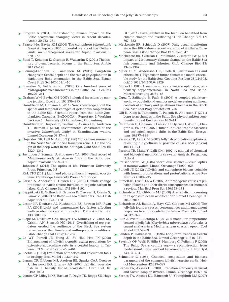
Fleming-Lehtinen & Laamanen (2012) found thatthe Baltic Sea Secchi depth cannot be linked solely tophytoplankton biomass due to a high backgroundlight attenuation. We approximated the backgroundlight attenuation from 123 observations of the attenu-ation coefficient of downwelling irradiance (K),chlorophyll (chl), and salinity (sal) made during 13cruises (Haraldsson et al. 2013) in the Baltic Properin 2009 and 2010 (Table 5). The reason for includingsalinity is that attenuation is known to be stronglyaffected by color dissolved organic matter (CDOM)originating from terrestrial and freshwater sour ces,and that light absorption is negatively linearlyrelated to salinity due to the dilution effect, withhigh-salinity water having lower light absorption(Aarup et al. 1996, Højerslev et al. 1996, Aksnes et al.2009). The regression analysis (Table 5) suggests alight attenuation of 0.64 m−1 of the Baltic Sea fresh-water sources (i.e. for sal = 0 and chl = 0), and furtherthat a water column with salinity of 8 to 9, which is

devoid of chlorophyll, has a background attenuationof 0.1 to 0.16 m−1. Use of the relationship S = 1.44/K(Kirk 2011) indicates a background Secchi disk depth(i.e. for chl = 0) of the present Baltic Sea of 10 to 15 m,which suggests that the Secchi depth of a water col-umn devoid of primary production is about twice thatof the current situation (6 m).

RESULTS

Predictions from the KtW model

We plotted the steady-state solutions as a functionof eutrophication (Fig. 3) for the loss rates and pre -dation coefficients in Tables 2 & 3. The degree ofeutrophication was converted into units of primaryproduction according to TZ = 0.09 (see Materials andMethods). For a primary production less than 32 g C

m−2 yr−1 (marked with arrow 1 inFig. 3), the KtW predicts that the massentering the system is too low to sustain cod and jellyfish. Above thisthreshold, cod enters and increaseswith increased eutrophi cation untilthe next threshold is reached at a primary production of 91 g C m−2 yr−1

(arrow 2). Here jellyfish enter, andfurther eutrophication leads to accu-mulation of jellyfish biomass, whilethe biomasses of the zooplankton andfishes remain unchanged. The pres-ent Baltic Sea (i.e. the observed bio-masses of Table 2) is marked witharrow 3 at a primary production of187 g C m−2 yr−1 (Wasmund et al. 2001).

78

Symbol Estimate Unit

Mass entering zooplankton (Z ) PZ 6.3 Mt C yr−1

Expressed per surface area 24.5 g C m−2 yr−1

Predation coefficient of jellyfish (J ) αJ 2113 m3 (g C)−1 yr−1

sprat/herring (F ) αF 505 m3 (g C)−1 yr−1

of cod (C ) αC 161 m3 (g C)−1 yr−1

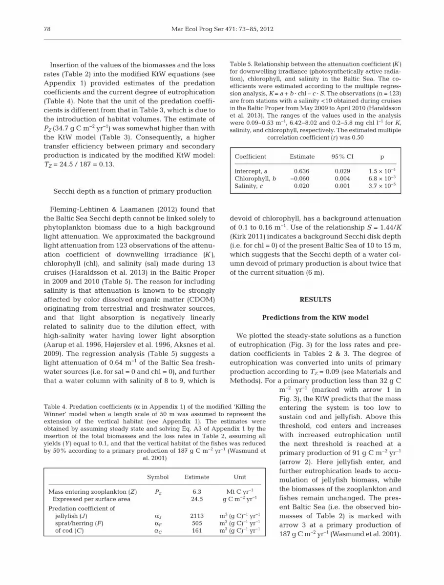
Table 4. Predation coefficients (α in Appendix 1) of the modified ‘Killing theWinner’ model when a length scale of 50 m was assumed to represent theextension of the vertical habitat (see Appendix 1). The estimates wereobtained by assuming steady state and solving Eq. A3 of Appendix 1 by theinsertion of the total biomasses and the loss rates in Table 2, assuming allyields (Y ) equal to 0.1, and that the vertical habitat of the fishes was reducedby 50% according to a primary production of 187 g C m−2 yr−1 (Wasmund et

al. 2001)

Coefficient Estimate 95% CI p

Intercept, a 0.636 0.029 1.5 × 10−4

Chlorophyll, b −0.060 0.004 6.8 × 10−3

Salinity, c 0.020 0.001 3.7 × 10−5

Table 5. Relationship between the attenuation coefficient (K)for downwelling irradiance (photosynthetically active radia-tion), chlorophyll, and salinity in the Baltic Sea. The co -efficients were estimated according to the multiple regres-sion analysis, K = a + b · chl – c · S. The observations (n = 123)are from stations with a salinity <10 obtained during cruisesin the Baltic Proper from May 2009 to April 2010 (Haraldssonet al. 2013). The ranges of the values used in the analysiswere 0.09−0.53 m−1, 6.42−8.02 and 0.2−5.8 mg chl l−1 for K,salinity, and chlorophyll, respecti vely. The estimated multiple

correlation coefficient (r ) was 0.50

Haraldsson et al.: Modeling fish and jellyfish relationships

Sensitivity

The existence of the 2 thresholds (Eqs. 3 and 6and arrows 1 and 2 in Fig. 3) is inherent to theKtW structure, but the estimated values of thesethresholds are sensitive to errors in the coefficientsof the model. From Table 6 it can be seen that theestimated threshold for jellyfish existence is in -creased from 91 to 149 g C m−2 yr−1 for a doublingof the cod biomass, or of the loss rate estimate thatwas used in the analysis (Table 2). The highestsensitivity of the predicted threshold is seen foruncertainties in the coefficients of the fishes, whilethe coefficients concerning zooplankton and jelly-fish do not affect the estimated threshold. Thislack of sensitivity to the zooplankton and jellyfishcoefficients is surprising. According to Eq. (3), themortality of jellyfish does affect the threshold inthe same way as cod mortality. However, a changein the jellyfish mortality also affects the predationcoefficient of jellyfish (also in Eq. 3) that cancelsout the effect on the calculated threshold. Never-theless, we emphasize that our Bal tic Sea applica-tion serves the purpose of illustrating the generalaspects of the KtW predictions rather than provid-ing accurate estimates.

Predicted effects of fishery

The 2 coefficients δF and δC are the fishery mortali-ties of sprat and herring or cod, respectively, andthe predicted effects from fishery can be assesseddirectly from the equations. From F* = δC/YC aC

(Eq. 2c), we see that the consequence of increasedcod fishery is a linear increase in F* (sprat and her-ring) at the expense of jellyfish according to J* = A –δC B (A and B are lumped coefficients of Eq. 2b).Decreased cod fishery leads to the opposite situationwhere the sprat and herring stocks decrease whilethat of the jellyfish increases. As noted above, andseen from Eq. (3), a decreased cod fishery also de -creases the eutrophication threshold for jellyfishentry to the system. Thus a general KtW implicationis that jellyfish abundance is stimulated by eutrophi-cation, but that this effect is counteracted by fisheryof the top predator in the KtW structure.

Decreased sprat and herring fishery results, notsurprisingly, in increased cod according to C* = aC

–1

(A – δF) (Eq. 2d, where A = YF aF δJ/YJaJ) and viceversa. More surprising, according to Eq. (2b), jelly-fish abundance is unaffected by changes in fisheryon its competitor. This insensitivity to fishing inten-sity might appear counterintuitive and is discussedbelow.

Predictions from the modified KtW model

The assumption that the habitat of the fishes isgradually reduced with increased eutrophicationleads to a 2-sided effect of eutrophication with anoptimal degree of eutrophication for which the fishbiomass is maximal (Fig. 4). Initially, the results are

79

Fig. 3. Steady-state solution of the ‘Killing the Winner’model as a function of eutrophication. Eutrophication isapproximated by annual primary production by assuming atransfer efficiency of TZ = 0.09 between primary producersand zooplankton (see ‘Materials and methods’). The solutionis given for the loss rates and the predation coefficientsgiven in Tables 2 & 3, respectively. Arrows: entry point ofcod (1), jellyfish (2) and the current state of the Baltic Sea (3)which corresponds to a primary production of 187 g C m−2

yr−1 (Wasmund et al. 2001)

Parameter 50% 200%

Zooplankton biomass 91 91Jellyfish biomass 91 91Sprat and herring biomass 74 123Cod biomass 62 149Jellyfish loss rate 91 91Sprat and herring loss rate 74 123Cod loss rate 62 149

Table 6. Sensitivity of a ‘Killing the Winner’ prediction forchanges in biomasses and loss rates of the different groups.Numbers are the calculated degree of eutrophication (g Cm−2 yr−1) required for jellyfish existence (i.e. threshold pro-vided by Eq. 3) when the specified input parameters were50 and 200% of the values used in the analysis (Table 2).The values used in the analysis gave an estimate of 91 g C

m−2 yr−1 (see ‘Results’)

Mar Ecol Prog Ser 471: 73–85, 2012

similar to the predictions of the basic KtW model(Fig. 3), with an increase in the sprat and herring bio-mass as a function of increased eutrophication. In thisphase the stimulating effect of increased mass (i.e.primary production) that enters the system overridesthe negative effect of a shrinking vertical habitat. Atthe entry point of cod (arrow 1 in Fig. 4), however, thecombined effect of habitat loss and cod predationresults in decreased sprat and herring biomass aseutrophication increases further. Cod reaches themaximal biomass at the entry point of jellyfish (arrow2 in Fig. 4), and the decrease thereafter is also causedby habitat deterioration. For the modified KtW thereis a steeper increase (~50%) in jellyfish biomass withincreased eutrophication than for the basic KtWwhich is associated with the concurrent decline inthe fish stocks in the modified KtW.

The maximal biomass of sprat and herring in themodified KtW (Fig. 4) is about twice the plateaureached in the basic KtW (Fig. 3). This difference isdue to methodological differences in the estimationof the predation coefficients. The biomasses for thecurrent Baltic Sea (Table 2), which is indicated byarrow 3 in Figs. 3 & 4, are the same in the 2 scenarios.Because the predation coefficients are estimatedfrom the values in Table 2, and the modified KtWassumes 50% habitat loss for this situation, the bio-mass becomes higher at a larger habitat size in thecase of the modified KtW model.

In Fig. 5, the results of the modified KtW are plottedas a function of Secchi depth instead of primary pro-duction. Here we see that the zooplanktivorous fishbiomass (sprat and herring) increases linearly withincreased water clarity (i.e. deeper Secchi depth)until a point where the diminishing primary produc-tion cannot sustain the zooplanktivorous biomassanymore and the biomass collapses accordingly. Thesame pattern is indicated for cod.

DISCUSSION

The extensive changes in the Baltic Sea (Table 1)make environmental analyses particularly challeng-ing. Climate-related changes such as increased seasurface temperature have been reported (Fonselius &Valderrama 2003, Mackenzie et al. 2007), and theBaltic Sea is considered one of the quickest-warmingseas worldwide (Belkin 2009). Detailed mechanistic(Österblom et al. 2007) and statistical (Casini et al.2008, 2009, Llope et al. 2011) dynamic models obvi-ously capture much more of the complexity of theBaltic Sea ecosystem than the steady-state KtWmodel. The role of jellyfish has not been explicitlyaddressed in such analyses, which is likely due tolack of jellyfish time series and lack of reports of massoccurrences similar to those occurrences that havebeen reported for e.g. the Black Sea (Llope et al.2011).

80

Fig. 4. Steady-state solution of the modified ‘Killing the Win-ner’ model as a function of eutrophication. Eutrophication isapproximated by annual primary production by assuming atransfer efficiency of TZ = 0.13 between primary producersand zooplankton (see ‘Materials and methods’). The solutionis given for the loss rates and the predation coefficientsgiven in Tables 2 & 4, respectively. Arrows: entry point ofcod (1), jellyfish (2), and the current state of the Baltic Sea(3), which corresponds to a primary production of 187 g C

m−2 yr−1 (Wasmund et al. 2001)

Fig. 5. Steady-state solution of the modified ‘Killing the Win-ner’ model given as a function of Secchi depth instead of pri-mary production as in Fig 4. Arrows: entry point of cod (1),jellyfish (2), and the current state of the Baltic Sea (3), which corresponds to a Secchi depth of 6 m (see ‘Materials and

methods’)

Haraldsson et al.: Modeling fish and jellyfish relationships

Our Baltic Sea application targets a particular envi-ronmental aspect, i.e. eutrophication and water clar-ity, and ignores others such as warming, hypoxia,and toxic pollutants. We acknowledge this limitationof our study, and our Baltic Sea application first of allserves the purpose of illustrating what we think arevaluable insights of the KtW model for the jellyfish−fish system. The KtW model has its main advantagein being generic, transparent, and analytically trac -table. Despite its simplicity, the KtW model is knownto capture many aspects of the relationship betweenmicrobial organisms (Winter et al. 2010). KtW fea-tures such as mass balance, competition for a com-mon resource, and tradeoff conflicts associated withinvestments in defense and resource acquisition arecrucial, not only for the microbial community, but fororganisms in general.

A fundamental assumption underlying the KtWpredictions in Figs. 3 & 4 is the framing of jellyfish asa defense specialist (Fig. 1). If this assumption is notwarranted, the KtW does not apply. The crucial pointis that the mortality coefficient of jellyfish can bespecified by a coefficient that is not seriously affectedby the dynamics of a top predator. This constant mortality coefficient is in contrast to that of the com-petition specialist, which indeed is affected by thedynamics of the top predator (Fig. 2).

The KtW model provides expectations, and poten-tially insights, that may appear surprising. It predictsa threshold criterion for the presence of jellyfish (i.e.the defense specialist) that connects to a particulardegree of eutrophication, which is modified by e.g.the mortality of the top predator. Increase in eutro -phication above this threshold results in more jelly-fish, but no further increase in its fish competitor(competition specialist) or the top predator (Figs. 3 &4). These predictions must be understood as emer-gent properties of the generic KtW structure (Fig. 1).Other predictions appear more trivial, e.g. thatdecreased fishery mortality of the top predator (cod)provides increased jellyfish abundance. Intuitively,this expectation can be linked to reduced food com-petition since the biomass of the competition special-ist (sprat and herring) is suppressed due to higherpredation from an elevated cod stock. The predictionthat the abundance of jellyfish is unaffected by spratand herring fishery, however, appears counterintu-itive. Intuitively, increased sprat and herring fisherywill lower these stocks, at least for a period of time,due to delays associated with maturation and repro-duction, and thereby leave more zooplankton for jellyfish growth. It is not obvious, however, whethersuch time delays would facilitate a permanent or a

temporary rise in jellyfish biomass. In any case, animportant limitation in our analysis is that the steady-state solution cannot account for such temporaldynamics.

The prediction that there are no negative effects ofan ever increasing eutrophication (i.e. Fig. 3) appearsunsound. This expectation is likely to be less realisticfor fish than for the microbial communities to whichKtW has primarily been applied (Winter et al. 2010),and it may be more important to address a 2-sidedeffect of eutrophication for higher than for lowertrophic levels.

Two-sided effect of eutrophication

The assumption that fish habitat is affected nega-tively by decreasing water clarity results in a linearincrease in fish biomass with increasing Secchi depthas long as the production of the system is sufficient tosupport such increase (i.e. up to arrow 1 for sprat andherring in Fig. 5). Evidence of such a linear relation-ship between fish biomass and Secchi depth hasbeen reported for the Black Sea (Aksnes 2007). Inthat study, Secchi depth was a surprisingly accuratepredictor of fish biomass over a 30 yr time series, anda Secchi depth shoaling of 1 m corresponded to adecrease of about 100 000 t of fish. Extrapolation sug-gested a critical Secchi depth of 4 to 5 m where thefish biomass became 0. No such critical Secchi depth,other than 0 m, was assumed in Fig. 5. If such criticalwater clarity is introduced to the model, a newthreshold will emerge. Water clarity lower than thecritical value would allow the presence of jellyfishand zooplankton only (not shown). Such an effect ofwater clarity might be a matter of future concernsince CDOM already makes a substantial contribu-tion to the relatively low water clarity of the BalticSea (Fleming-Lehtinen & Laamanen 2012), and asubstantial increase in CDOM loads is expected dueto increased warming and precipitation (Larsen et al.2011)

Unfortunately, lack of time series of jellyfish pro-hibits a close inspection of how the KtW model com-pares with the development in the Baltic Sea. Thestudy of Möller (1980) indicates a jellyfish biomass of24 Mt wet weight (WW) in 1978 (Table 7). This num-ber is less than the estimate for the current situation(61 Mt WW, Table 2), but these estimates do notallow a robust statistical comparison. In Table 7 wehave also provided the average biomasses of zoo-plankton, sprat and herring, and cod in the period1974 to 1979, which can be compared with the aver-

81

Mar Ecol Prog Ser 471: 73–85, 2012

ages for the period 2000 to 2009 (Table 2). It can beconcluded that the fish stocks were significantlyhigher in the early period while the zooplankton bio-mass estimates were similar. Hence, the direction ofthe changes in all 4 groups is consistent with theexpectation of the modified KtW (Figs. 4 & 5) if Sec-chi depth was shallower in the late than in the earlyperiod. The study of Fleming-Lehtinen & Laamanen(2012, their Fig. 3) in deed suggests a 1 to 2 m reduc-tion in Secchi depth for most of the sub-basins in theBaltic Sea since the 1970s.

According to the KtW predictions, it might be spec-ulated that the current high cod fishery (Table 2) con-tributes to a suppression of the Baltic Sea jel lyfishbiomass, and that a shift towards more cod, and lesssprat and herring, would lead to increased jellyfishabundance. Nevertheless, the KtW expectations pre-sented in our study obviously need to be confrontedwith observations in future studies. Due to a generallack of reliable time series for jellyfish, future studiescould involve ‘space for time’ sampling, i.e. samplingfrom different locations that reflect a gradient ineutrophication and water clarity.

Acknowledgements. We thank M. Casini for providing zoo-plankton biomass data. This work is a contribution to BalticZooplankton Cascades (BAZOOCA) funded by BalticOrganizations Network for funding Science, European Eco-nomic Interest Grouping (BONUS, EEIG), and the SwedishResearch Council for Environment, Agricultural Sciences,and Spatial Planning (FORMAS) project 210-2008-1882. Wereceived additional support from the EU-ERC projectMINOS (ref no 250254) and the Norwegian Research Coun-cil (project no 196444).

LITERATURE CITED

Aarup T, Holt N, Højerslev NK (1996) Optical measurementsin the North Sea-Baltic Sea transition zone. 2. Watermass classification along the Jutland west coast fromsalinity and spectral irradiance measurements. ContShelf Res 16: 1343−1353

Acuña JL, López-Urrutia Á, Colin S (2011) Faking giants: the evolution of high prey clearance rates in jellyfishes.Science 333: 1627−1629

Aksnes DL (2007) Evidence for visual constraints in largemarine fish stocks. Limnol Oceanogr 52: 198−203

Aksnes DL, Utne ACW (1997) A revised model of visualrange in fish. Sarsia 82: 137−147

Aksnes DL, Dupont N, Staby A, Fiksen Ø, Kaartvedt S, AureJ (2009) Coastal water darkening and implications formesopelagic regime shifts in Norwegian fjords. Mar EcolProg Ser 387: 39−49

Alheit J, Möllmann C, Dutz J, Kornilovs G, Loewe P,Mohrholz V, Wasmund N (2005) Synchronous ecologicalregime shifts in the central Baltic and the North Sea inthe late 1980s. ICES J Mar Sci 62: 1205−1215

Andersen JH, Axe P, Backer H, Carstensen J and others(2011) Getting the measure of eutrophication in theBaltic sea: towards improved assessment principles andmethods. Biogeochemistry 106: 137−156

Arrhenius F, Hansson S (1993) Food consumption of larval,young and adult herring and sprat in the Baltic Sea. MarEcol Prog Ser 96: 125−137

Backer H, Leppanen JM (2008) The HELCOM system of avision, strategic goals and ecological objectives: imple-menting an ecosystem approach to the management ofhuman activities in the Baltic Sea. Aquat Conserv 18: 321−334

Barz K, Hirche HJ (2005) Seasonal development of scypho-zoan medusae and the predatory impact of Aurelia auritaon the zooplankton community in the Bornholm basin(central Baltic Sea). Mar Biol 147: 465−476

Belkin IM (2009) Rapid warming of large marine ecosys-tems. Prog Oceanogr 81: 207−213

Brodeur RD, Sugisaki H, Hunt GL Jr (2002) Increases injelly fish biomass in the Bering Sea: implications for theecosystem. Mar Ecol Prog Ser 233: 89−103

Brotz LL, Cheung WWL, Kleisner K, Pakhomov E, Pauly D(2012) Increasing jellyfish populations: trends in LargeMarine Ecosystems. Hydrobiologia 690: 3−20

Casini M, Lövgren J, Hjelm J, Cardinale M, Molinero JC,Kornilovs G (2008) Multi-level trophic cascades in aheavily exploited open marine ecosystem. Proc R SocLond B Biol Sci 275: 1793−1801

Casini M, Hjelm J, Molinero JC, Lövgren J and others(2009) Trophic cascades promote threshold-like shiftsin pelagic marine ecosystems. Proc Natl Acad Sci USA106: 197−202

Condon RH, Graham WM, Duarte CM, Pitt KA and others(2012) Questioning the rise of gelatinous zooplankton inthe world’s oceans. Bioscience 62: 160−169

Daskalov GM, Grishin AN, Rodionov S, Mihneva V (2007)Trophic cascades triggered by overfishing reveal possi-ble mechanisms of ecosystem regime shifts. Proc NatlAcad Sci USA 104: 10518−10523

Decker MB, Breitburg DL, Purcell JE (2004) Effects of lowdissolved oxygen on zooplankton predation by thecteno phore Mnemiopsis leidyi. Mar Ecol Prog Ser 280: 163−172

Diaz RJ, Rosenberg R (2008) Spreading dead zones and con-sequences for marine ecosystems. Science 321: 926−929

Dupont N, Aksnes DL (2010) Simulation of optically condi-tioned retention and mass occurrences of Periphylla peri-phylla. J Plankton Res 32: 773−783

Eggers DM (1977) Nature of prey selection by planktivorousfish. Ecology 58: 46−59

82

Group Biomass Source

Zooplankton (Z) 4.2 ± 0.8 Casini et al. (2008)Jellyfish (J ) 24.2 Möller (1980)Sprat and 4.02 ± 0.23 Swedish Agency for

herring (F ) Marine and Water Cod (C ) 0.73 ± 0.18 Management (2010)

Table 7. Biomasses (mean ± SD; wet weight in Mt) in theBaltic Sea for the period 1974 to 1979, except for jellyfish,which represent sampling in September 1978 (the biomass

of jellyfish in Table 2 also represents September)

⎫⎬⎭

Haraldsson et al.: Modeling fish and jellyfish relationships

Elmgren R (2001) Understanding human impact on theBaltic ecosystem: changing views in recent decades.Ambio 30: 222−231

Faasse MA, Bayha KM (2006) The ctenophore Mnemiopsisleidyi A. Agassiz 1865 in coastal waters of the Nether-lands: an unrecognized invasion? Aquat Invasions 1: 270−277

Finni T, Kononen K, Olsonen R, Wallström K (2001) The his-tory of cyanobacterial blooms in the Baltic Sea. Ambio30: 172−178

Fleming-Lehtinen V, Laamanen M (2012) Long-termchanges in Secchi depth and the role of phytoplankton inexplaining light attenuation in the Baltic Sea. EstuarCoast Shelf Sci 102-103: 1−10

Fonselius S, Valderrama J (2003) One hundred years ofhydrographic measurements in the Baltic Sea. J Sea Res49: 229−241

Graham WM, Bayha KM (2007) Biological invasions by mar-ine jellyfish. Ecol Stud 193: 239−255

Haraldsson M, Hansson L (2011) New knowledge about thespatial and temporal changes of gelatinous zooplanktonin the Baltic Sea. Scientific report from the ‘Baltic Zoo-plankton Cascades (BAZOOCA)’. Report no. 2. Workingpackage 1. University of Gothenburg, Gothenburg

Haraldsson M, Jaspers C, Tiselius P, Aksnes DL, AndersenT, Titelman J (2013) Environmental constraints of theinvasive Mnemiopsis leidyi in Scandinavian waters. Limnol Oceanogr 58:37–48

Højerslev NK, Holt N, Aarup T (1996) Optical measurementsin the North Sea-Baltic Sea transition zone. 1. On the ori-gin of the deep water in the Kattegat. Cont Shelf Res 16: 1329−1342

Javidpour J, Sommer U, Shiganova TA (2006) First record ofMnemiopsis leidyi A. Agassiz 1865 in the Baltic Sea.Aquat Invasions 1: 299−302

Johnsen S (2012) The optics of life. Princeton UniversityPress, Princeton, NJ

Kirk JTO (2011) Light and photosynthesis in aquatic ecosys-tems. Cambridge University Press, Cambridge

Larsen S, Andersen T, Hessen DO (2011) Climate changepredicted to cause severe increase of organic carbon inlakes. Glob Change Biol 17: 1186−1192

Leppäkoski E, Gollasch S, Gruszka P, Ojaveer H, Olenin S,Panov V (2002) The Baltic — a sea of invaders. Can J FishAquat Sci 59: 1175−1188

Lester NP, Dextrase AJ, Kushneriuk RS, Rawson MR, RyanPA (2004) Light and temperature: key factors affectingwalleye abundance and production. Trans Am Fish Soc133: 588−605

Llope M, Daskalov GM, Rouyer TA, Mihneva V, Chan KS,Grishin AN, Stenseth NC (2011) Overfishing of top pre -dators eroded the resilience of the Black Sea systemregardless of the climate and anthropogenic conditions.Glob Change Biol 17: 1251−1265

Lo WT, Purcell JE, Hung JJ, Su HM, Hsu PK (2008)Enhancement of jellyfish (Aurelia aurita) populations byextensive aquaculture rafts in a coastal lagoon in Tai-wan. ICES J Mar Sci 65: 453−461

Loehle C (1983) Evaluation of theories and calculation toolsin ecology. Ecol Model 19: 239−247

Lynam CP, Gibbons MJ, Axelsen BE, Sparks CAJ, CoetzeeJ, Heywood BG, Brierley AS (2006) Jellyfish overtakefish in a heavily fished ecosy stem. Curr Biol 16: R492−R493

Lynam CP, Lilley MKS, Bastian T, Doyle TK, Beggs SE, Hays

GC (2011) Have jellyfish in the Irish Sea benefited fromclimate change and overfishing? Glob Change Biol 17: 767−782

Mackenzie BR, Schiedek D (2007) Daily ocean monitoringsince the 1860s shows record warming of northern Euro-pean Seas. Glob Change Biol 13: 1335−1347

Mackenzie BR, Gislason H, Möllmann C, Köster FW (2007)Impact of 21st century climate change on the Baltic Seafish community and fisheries. Glob Change Biol 13: 1348−1367

Meier HEM, Andersson HC, Eilola K, Gustafsson BG andothers (2011) Hypoxia in future climates: a model ensem-ble study for the Baltic Sea. Geophys Res Lett 38: L24608,doi:10.1029/2011GL049929

Möller H (1980) A summer survey of large zooplankton, par-ticularly scyphomedusae, in North Sea and Baltic.Meeresforschung 28: 61−68

Oguz T, Salihoglu B, Fach B (2008) A coupled plankton−anchovy population dynamics model assessing nonlinearcontrols of anchovy and gelatinous biomass in the BlackSea. Mar Ecol Prog Ser 369: 229−256

Olli K, Klais R, Tamminen T, Ptacnik R, Andersen T (2011)Long term changes in the Baltic Sea phytoplankton com-munity. Boreal Environ Res 16: 3−14

Österblom H, Hansson S, Larsson U, Hjerne O, Wulff F, Elm-gren R, Folke C (2007) Human-induced trophic cascadesand ecological regime shifts in the Baltic Sea. Ecosys-tems 10: 877−889

Parsons TR, Lalli CM (2002) Jellyfish population explosions: revisiting a hypothesis of possible causes. Mer (Tokyo)40: 111−121

Parsons TR, Maita Y, Lalli CM (1992) A manual of chemicaland biological methods for seawater analysis. Pergamon,Oxford

Preisendorfer RW (1986) Secchi disk science — visual opticsof natural waters. Limnol Oceanogr 31: 909−926

Purcell JE (2012) Jellyfish and ctenophore blooms coincidewith human proliferations and perturbations. Annu RevMar Sci 4: 209−235

Purcell JE, Uye S, Lo WT (2007) Anthropogenic causes of jel-lyfish blooms and their direct consequences for humans: a review. Mar Ecol Prog Ser 350: 153−174

Richardson AJ, Gibbons MJ (2008) Are jellyfish increasingin response to ocean acidification? Limnol Oceanogr 53: 2040−2045

Richardson AJ, Bakun A, Hays GC, Gibbons MJ (2009) Thejellyfish joyride: causes, consequences and managementresponses to a more gelatinous future. Trends Ecol Evol24: 312−322

Ruiz J, Prieto L, Astorga D (2012) A model for temperaturecontrol of jellyfish (Cotylorhiza tuberculata) outbreaks: acausal analysis in a Mediterranean coastal lagoon. EcolModel 233: 59−69

Sanden P, Håkansson B (1996) Long-term trends in Secchidepth in the Baltic Sea. Limnol Oceanogr 41: 346−351

Savchuk OP, Wulff F, Hille S, Humborg C, Pollehne F (2008)The Baltic Sea a century ago — a reconstruction frommodel simulations, verified by observations. J Mar Syst74: 485−494

Schneider G (1988) Chemical composition and biomassparameters of the common jellyfish Aurelia aurita. Hel-gol Meersunters 42: 319−327

Sørnes TA, Aksnes DL (2004) Predation efficiency in visualand tactile zooplanktivores. Limnol Oceanogr 49: 69−75

Sørnes TA, Aksnes DL, Båmstedt U, Youngbluth MJ (2007)

83

Mar Ecol Prog Ser 471: 73–85, 2012

Causes for mass occurrences of the jellyfish Periphyllaperiphylla: a hypothesis that involves optically condi-tioned retention. J Plankton Res 29: 157−167

Sparholt H (1994) Fish species interactions in the Baltic Sea.Dana 10: 131−162

Struck U, Emeis KC, Voss M, Christiansen C, Kunzendorf H(2000) Records of southern and central Baltic Sea eutro -phication in δ13C and δ15N of sedimentary organic matter.Mar Geol 164: 157−171

Swedish Agency for Marine and Water Management (2010)Fiskebestånd och miljö i hav och sötvatten. Resurs- ochmiljööversikt 2010. Fiskeriverket. Available at www.hav-ochvatten.se

Tendal OS, Jensen KR, Riisgård HU (2007) Invasive cteno -phore Mnemiopsis leidyi widely distributed in Danishwaters. Aquat Invasions 2: 455−460

Thingstad TF, Strand E, Larsen A (2010) Stepwise buildingof plankton functional type (PFT) models: a feasible routeto complex models? Prog Oceanogr 84: 6−15

Thuesen EV, Rutherford LD, Brommer PL, Garrison K,Gutowska MA, Towanda T (2005) Intragel oxygen pro-

motes hypoxia tolerance of scyphomedusae. J Exp Biol208: 2475−2482

Thurow F (1997) Estimation of the total fish biomass in theBaltic Sea during the 20th century. ICES J Mar Sci 54: 444−461

Wasmund N, Andrushaitis A, Lysiak-Pastuszak E, Müller-Karulis B and others (2001) Trophic status of the south-eastern Baltic Sea: a comparison of coastal and openareas. Estuar Coast Shelf Sci 53: 849−864

Wasmund N, Göbel J, von Bodungen B (2008) 100-years-changes in the phytoplankton community of Kiel Bight(Baltic Sea). J Mar Syst 73: 300−322

Weisse T, Gomoiu MT (2000) Biomass and size structure ofthe scyphomedusa Aurelia aurita in the northwesternBlack Sea during spring and summer. J Plankton Res 22: 223−239

Winter C, Bouvier T, Weinbauer MG, Thingstad TF (2010)Trade-offs between competition and defense specialistsamong unicellular planktonic organisms: the ‘Killing theWinner’ hypothesis revisited. Microbiol Mol Biol Rev 74: 42−57

84

Haraldsson et al.: Modeling fish and jellyfish relationships 85

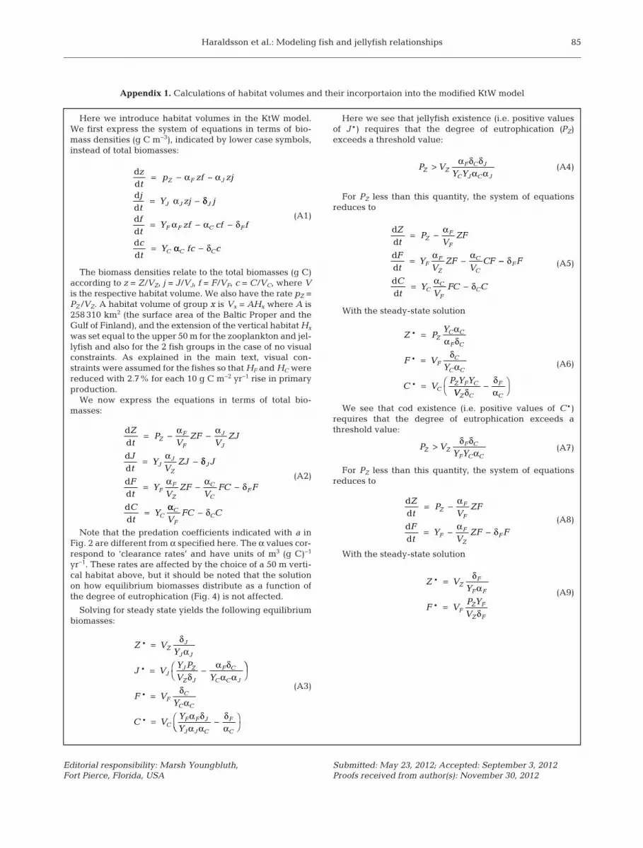
Appendix 1. Calculations of habitat volumes and their incorportaion into the modified KtW model

Here we introduce habitat volumes in the KtW model.We first express the system of equations in terms of bio-mass densities (g C m−3), indicated by lower case symbols,instead of total biomasses:

(A1)

The biomass densities relate to the total biomasses (g C)according to z = Z/VZ, j = J/VJ, f = F/VF, c = C/VC, where Vis the respective habitat volume. We also have the rate pZ =PZ/VZ. A habitat volume of group x is Vx = AHx where A is258 310 km2 (the surface area of the Baltic Proper and theGulf of Finland), and the extension of the vertical habitat Hx

was set equal to the upper 50 m for the zooplankton and jel-lyfish and also for the 2 fish groups in the case of no visualconstraints. As explained in the main text, visual con-straints were assumed for the fishes so that HF and HC werereduced with 2.7% for each 10 g C m−2 yr−1 rise in primaryproduction.

We now express the equations in terms of total bio-masses:

(A2)

Note that the predation coefficients indicated with a inFig. 2 are different from α specified here. The α values cor-respond to ‘clearance rates’ and have units of m3 (g C)−1

yr−1. These rates are affected by the choice of a 50 m verti-cal habitat above, but it should be noted that the solutionon how equilibrium biomasses distribute as a function ofthe degree of eutrophication (Fig. 4) is not affected.

Solving for steady state yields the following equilibriumbiomasses:

(A3)

Here we see that jellyfish existence (i.e. positive valuesof J*) requires that the degree of eutrophication (PZ)exceeds a threshold value:

(A4)

For PZ less than this quantity, the system of equationsreduces to

(A5)

With the steady-state solution

(A6)

We see that cod existence (i.e. positive values of C*)requires that the degree of eutrophication exceeds athreshold value:

(A7)

For PZ less than this quantity, the system of equationsreduces to

(A8)

With the steady-state solution

(A9)

dddd

zt

p zf zj

jt

Y zj

Z F J

J J

–= −

= −

α α

α δδ

α α δ

J

F F C F

C

j

ft

Y zf cf f

ct

Y

dddd

= − −

= αα δC Cfc c−

dd

dd

Zt

PV

ZFV

ZJ

Jt

YV

ZJ

ZF

F

J

J

JJ

Z

= − −

= −

α α

α δδ

α α δ

J

FF

Z

C

CF

C

J

Ft

YV

ZFV

FC F

Ct

Y

dd

dd

= − −

= αα δC

FCV

FC C−

Z VY

J VY PV Y

ZJ

J J

JJ Z

Z J

F C

C C J

*

*

=

= −⎛⎝

δα

δα δα α

⎞⎞⎠

=

= −⎛

F VY

C VYY

FC

C C

CF F J

J J C

F

C

*

*

δα

α δα α

δα⎝⎝

⎞⎠

P VY YZ Z

F C J

C J C J

> α δ δα α

dd

dd

Zt

PV

ZF

Ft

YV

ZFV

CF

ZF

F

FF

Z

C

C

= −

= −

α

α α −−

= −

δ

α δ

F

CC

FC

F

Ct

YV

FC Cdd

Z PY

F VY

C VP Y Y

ZC C

F C

FC

C C

CZ F C

*

*

*

=

=

=

αα δ

δα

VVZ C

F

Cδδα

−⎛⎝

⎞⎠

P VY YZ Z

F C

F C C

> δ δα

dd

dd

Zt

PV

ZF

Ft

YV

ZF F

ZF

F

FF

ZF

= −

= − −

α

α δ

Z VY

F VP YV

ZF

F F

FZ F

Z F

*

*

=

=

δα

δ

Editorial responsibility: Marsh Youngbluth, Fort Pierce, Florida, USA

Submitted: May 23, 2012; Accepted: September 3, 2012Proofs received from author(s): November 30, 2012