DI

SC

US

SI

ON

P

AP

ER

S

ER

IE

S

Forschungsinstitut zur Zukunft der ArbeitInstitute for the Study of Labor

Relative Income, Redistribution and Well-being

IZA DP No. 5241

October 2010

Felix FitzRoyMichael Nolan

Relative Income,

Redistribution and Well-being

Felix FitzRoy University of St Andrews

and IZA

Michael Nolan University of Hull

Discussion Paper No. 5241 October 2010

IZA

P.O. Box 7240 53072 Bonn

Germany

Phone: +49-228-3894-0 Fax: +49-228-3894-180

E-mail: iza@iza.org

Any opinions expressed here are those of the author(s) and not those of IZA. Research published in this series may include views on policy, but the institute itself takes no institutional policy positions. The Institute for the Study of Labor (IZA) in Bonn is a local and virtual international research center and a place of communication between science, politics and business. IZA is an independent nonprofit organization supported by Deutsche Post Foundation. The center is associated with the University of Bonn and offers a stimulating research environment through its international network, workshops and conferences, data service, project support, research visits and doctoral program. IZA engages in (i) original and internationally competitive research in all fields of labor economics, (ii) development of policy concepts, and (iii) dissemination of research results and concepts to the interested public. IZA Discussion Papers often represent preliminary work and are circulated to encourage discussion. Citation of such a paper should account for its provisional character. A revised version may be available directly from the author.

IZA Discussion Paper No. 5241 October 2010

ABSTRACT

Relative Income, Redistribution and Well-being* In a model with heterogeneous workers and both intensive and extensive margins of employment, we consider two systems of redistribution: a universal basic income, and a categorical unemployment benefit. Well-being depends on own-consumption relative to average employed workers’ consumption, and concern for relativity is a parameter that affects model outcomes. While labour supply incurs positive marginal disutility, we allow negative welfare effects of unemployment. We also compare Rawlsian and utilitarian welfare in general equilibrium under the polar opposite transfer systems, with varying concern for relativity. Basic income Pareto dominates categorical benefits with moderate concern for relativity in both cases. JEL Classification: H20, D40 Keywords: relative income, redistribution, basic income, unemployment benefits,

happiness, well-being Corresponding author: Felix FitzRoy School of Economics and Finance University of St Andrews St Andrews KY16 9AL Scotland United Kingdom E-mail: frf@st-andrews.ac.uk

* An early version of this paper was presented in Bristol at the 2010 Annual Conference of the Work and Pensions Economics Group. Thanks are due to participants there, especially Tim Barmby, and to John Beath, Jim Jin, and David Ulph for discussions on related issues. A standard disclaimer applies.

2

1. Introduction

Evidence on the importance of relative income in subjective well-being (SWB) has

been accumulating rapidly, as summarized in the most comprehensive study to-date by

Layard et al (2010), or recent reviews by Clark et al (2008), Frey (2008), and Oswald (2009).

Appropriate reference income has a highly significant, negative effect on well-being similar

in magnitude to the effect of own income, after controlling for many personal characteristics.

The externality involved implies that redistributive taxation is less distortionary than

otherwise, and that tax rates should rise with concern for relativity1. Following the early study

of relative income by Boskin and Sheshinski (1978), subsequent work in this area has also

usually neglected the participation decision – whether to work or rely on benefits – which

empirical evidence shows to be most responsive to tax and wage incentives (Immervoll et al,

2007).

In contrast, most theoretical studies of redistribution and welfare in a general

equilibrium framework neglect the importance of relative income for well-being, and assume

a universal lump-sum transfer or basic income for all. This form of transfer has attractive

theoretical properties (Atkinson, 1995), but is far removed from practical welfare systems.

These invariably try to target the most needy, such as the unemployed or low-wage workers,

with categorical benefits that are withdrawn as earnings increase, thus generating often very

high effective marginal rates of tax, which can create a ‘poverty trap’ or disincentive to work.

Providing an adequate basic income for all, including the majority who are above the poverty

level, has generally seemed to require unacceptably high rates of taxation, but recent

microeconomic simulations show that a basic income can dominate other welfare systems

under realistic assumptions for some countries, including low observed labour supply

1 These results also help to explain the ‘Easterlin Paradox’ or lack of correlation between long term economic growth and changes in average happiness or SWB in advanced economies, in contrast to the positive, short term relationship and cross-sectional correlation between income and SWB (Easterlin, 1974; Easterlin and Angelescu, 2009; Layard et al, 2010). Subjective well-being is also strongly correlated with many objective indicators of quality of life (Oswald and Wu, 2010).

3

elasticities for the full time employed, and high participation response (Colombino et al,

2010). In a model focussing mainly on the participation decision, FitzRoy and Jin (2010) find

that basic income is generally preferred by a majority to categorical benefits. However these

models do not explicitly include concern for relative income, which has not yet been widely

incorporated into standard theories of optimal taxation and public economics (Kaplow,

2008)2.

Here we follow Layard’s (1980, 2006) call to systematically incorporate the widely

observed concern for relative income into the public economics of taxation and redistribution.

We differ from most previous contributions by developing an explicit comparison of the

welfare consequences of the two fundamental alternative modes of redistribution – basic

income and categorical benefits – in a simple general equilibrium model with heterogeneous

workers, including concern for relative income and income effects, and voluntary

unemployment. We find a surprising Pareto dominance of the basic income system with even

slight concern for relativity, and also that optimal tax and unemployment increase with

concern for relativity, under both Rawlsian and utilitarian social objectives.

These issues are of vital importance as poverty and unemployment increase in the

aftermath of recession. In the existing literature, there is extensive discussion of welfare

reform to encourage low wage employment and remove poverty traps, but little

acknowledgement of the role of relative income in comparing welfare consequences of

differing policy goals and models of redistribution, or the potential of a universal basic

income. The widely recognised tendency for economic policy-making to lag behind

developments in academic economics serves to add to the urgency of the situation. Layard

2 Pioneering exceptions include Oswald (1983), and Kanbur and Tuomala (2009), with optimal non-linear taxation. Beath and FitzRoy (2009) consider a related model with categorical benefits, a public good, flat taxes and a narrower reference income, and hence obtain some different results in this case, but this approach is not appropriate for modelling basic income and making the comparisons pursued here. Eaton and Eswaran (2009) include a ‘relative consumption externality’ from a Veblen good in a model of homogenous households (without redistribution), and a lump-sum tax to fund a public good.

4

(2005, 2006, 2009), Oswald (2009), Stiglitz et al (2010), and many others have emphasised

the need for policy to focus on the goal of happiness or subjective well-being, rather than

exclusive concern with average GDP (growth). In so-doing, important issues to consider

include relative income, basic income to avoid the ‘poverty trap’, taxation as an instrument to

discourage excessive effort, redistribution and social interactions.

For tractability, we restrict attention to linear or flat taxes, which may be a reasonable

approximation to optimal taxes. Thus Mankiw et al (2009, p. 2) suggest that “ A flat tax, with

a universal lump-sum transfer, could be close to optimal”, although Colombino et al (2010)

do find welfare gains from progressive taxes, using empirically-supported low labour supply

elasticities for full time employees, in contrast to much previous literature on optimal

taxation. The latter generally finds high marginal rates on low earners to be optimal, to ‘phase

out’ a universal transfer, followed by lower rates on higher earners to encourage labour

supply. The withdrawal of categorical benefits for full-time workers thus appears to

approximate at least part of the optimal tax schedule, though there are also important

differences (Kaplow, 2008).

The plan of the paper is to develop the benchmark general equilibrium model with a

universal basic income in section 2, and corresponding results with categorical

unemployment benefits in section 3. Most comparisons between the two systems and

dependence on optimally chosen parameters cannot be obtained analytically, so we present

the results of extensive numerical simulations of the main relationships (including the plots

themselves) in section 4. Conclusions are summarized in a final section 5.

2. A model with universal basic income

5

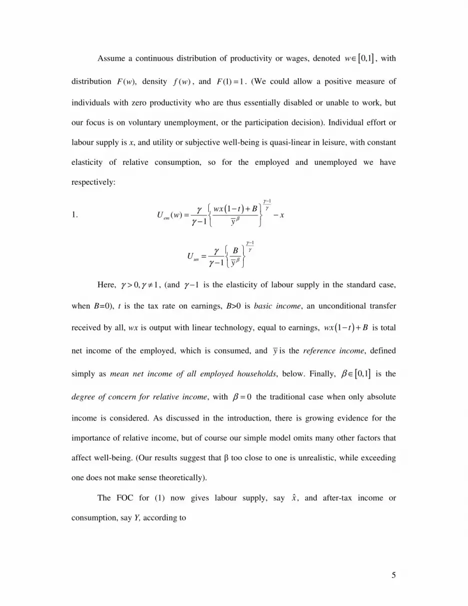
Assume a continuous distribution of productivity or wages, denoted [ ]0,1w∈ , with

distribution ( ),F w density ( )f w , and (1) 1F = . (We could allow a positive measure of

individuals with zero productivity who are thus essentially disabled or unable to work, but

our focus is on voluntary unemployment, or the participation decision). Individual effort or

labour supply is x, and utility or subjective well-being is quasi-linear in leisure, with constant

elasticity of relative consumption, so for the employed and unemployed we have

respectively:

1. ( )

1

1( )

1em

wx t BU w x

y

γγ

βγ

γ

−

− +� �= −� �− � �

1

1un

BU

y

γγ

βγ

γ

−

� �= � �− � �

Here, 0, 1γ γ> ≠ , (and 1γ − is the elasticity of labour supply in the standard case,

when B=0), t is the tax rate on earnings, B>0 is basic income, an unconditional transfer

received by all, wx is output with linear technology, equal to earnings, ( )1wx t B− + is total

net income of the employed, which is consumed, and y is the reference income, defined

simply as mean net income of all employed households, below. Finally, [ ]0,1β ∈ is the

degree of concern for relative income, with 0β = the traditional case when only absolute

income is considered. As discussed in the introduction, there is growing evidence for the

importance of relative income, but of course our simple model omits many other factors that

affect well-being. (Our results suggest that � too close to one is unrealistic, while exceeding

one does not make sense theoretically).

The FOC for (1) now gives labour supply, say x̂ , and after-tax income or

consumption, say Y, according to

6

2. ( )1

(1 )ˆ(1 )w t

wx t B Yy

γ γ

β γ −

−− + ≡ =

The positive basic income means that households with some positive marginal wage,

say m, will supply zero effort, and these and all other households with lower wages will be

voluntarily unemployed. Thus m is the effective minimum wage for employment, or strictly,

the lower bound, and from (2) it is given by

3. ( )1(1 )m t By β γγ γ −− = The number (or share) of the unemployed is thus F(m). Now using (2) and (3) we can

define mean, net income (or consumption) of the employed as follows:

4. ( )( ) ( ) ( )( )

1 1

1

1ˆ1 ( 1 )

m m

w ty F m wx t B dF dF

y

γγ

β γ −

−− = − + =� �

So we have average income as a function of m and t:

5. ( ) ( )( )1 1 11 ( )

G m ty

F m

γβ γ+ − −

=−

where ( ) ( )1

m

G m w f w dwγ≡ � and ( ) ( )G m m f mγ′ = − .

Next, the government budget is defined by equating tax revenue with redistributive

expenditure on the basic income for the unit population, so we obtain benefits as a function of

m and t, say

6. ( )1

ˆ,m

B m t t wxdF= �

Using (2) yields

7. ( ) ( )( ) ( )( ) ( )1

1, 1

t tB m t tF m G m

y

γ

β γ −

−− =

Next we incorporate the incentive-compatibility condition (3) for the marginal wage.

Then it is convenient to consider this minimum employment wage as the policy variable, and

7

derive the equilibrium tax rate, say ( )t̂ m , consistent with a given, incentive compatible

choice of minimum wage and the balanced-budget level of basic income by substituting for B

from (3) to give

8. ( ) ( ) ( )ˆ ,

mt m

m F m G m

γ

γγ =+

It is easy to verify that this is an increasing function of m, and a decreasing function of �, and

so could be inverted to give the minimum wage as an implicit function of the tax. It is thus

convenient to consider the minimum wage as the government’s policy instrument.

Now we can find general equilibrium mean, net income (or consumption), and basic

income, defined in the obvious way when the equilibrium tax is substituted into (5) and (7),

as functions of the minimum wage. From these two equations we get

9. ( ) ( )( ) ( )1

1 1ˆ1ˆ

1 ( )

G m ty m

F m

γ β γ+ −� �−� �= � �−� �� �

and from (3),

10. ( ) ( )1

ˆ(1 )ˆˆ

m tB m

y

γ γ

β γ −

−=

Notice that this has the same form as (3), but now we have substituted the equilibrium tax and

average income.

Then we can obtain the equilibrium individual income, effort and utility of the

employed and unemployed respectively as functions of the policy instrument, m, and the

individual wage, using (8) and (9)

( ) ( )

( ) ( )( )

1

1 1

1

ˆ(1 )ˆ , ,ˆ

ˆ ˆ1 ˆ1ˆ ,ˆˆ ˆ1

w tY m w

y

w t B m tx m w w

y w yw t

γ γ

β γ

γ γγγ

β β

−

− −−

−=

� �− � �� �−� �= − = −� � � �� �− � �� �� �� �

11.

8

( ) ( )1

11ˆ ˆ1ˆ ˆ , ,ˆ ˆ1 1un em

B w m tU m U m w

y w y

γγγ γγ

β βγ

γ γ

−−−� � � � � �−� �= = +� � � � � �− −� � � �� �� �

We summarize the main conclusions from these expressions as

Proposition 1:

For given m, individual labour supply in general equilibrium increases with the wage (though

not necessarily when � < 1, a case we do not consider further), as does the well-being of the

employed, ( which corresponds to empirical findings). For given m and w, equilibrium mean

income and individual effort increase with concern for relativity.

Intuitively, increasing concern means that other individuals’ greater effort creates a

larger externality, which in turn generates more offsetting effort by raising the marginal

return to effort. In the traditional case of zero concern for relative income, we see that

benefits first increase and then decline with unemployment or the minimum wage in a

standard Laffer curve. If m is small, the wage elasticity of labour supply for those in work is

approximately � – 1, which empirical evidence suggests is small for full-time workers. The

general case is too complicated for analytical solution.

3. Categorical benefits

A basic income to replace other benefits has not yet been introduced in practice, and

redistribution mainly targets the unemployed and the lowest paid workers. We explore this

alternative in the simplest way by assuming a fixed transfer for the non-employed, which is

lost when any labour is supplied, thus imposing a high marginal tax rate on low wage

workers who are just above effective minimum wage, and hence only slightly better off

working. While this neglects the complications of ‘tapered’ withdrawal of transfers as

earnings increase, it captures (in a tractable approximation) the basic feature of existing

welfare systems, that most of the employed do not receive transfers, and is closer to reality

9

than the universal basic income which is widely used in theoretical models. We thus drop

benefits in the utility of the employed in (1) and from the FOCs obtain labour supply, say

12. ( ) 11w t

xy

γ

β

−

∗ −� �= � �� �

Note that this yields the same after-tax earnings, ( )1wx t∗ − , as with basic income in (2), for a

given reference income. Clearly, 1γ < implies backward-bending labour supply, the less

plausible case because work time and earnings are strongly correlated in cross-section. Utility

from work at this wage and optimal labour supply is then:

13. ( ) 111

1em

w tU

y

γ

βγ

−

∗ −� �= � �− � �

The unemployed have utility from consumption of unemployment benefits, here denoted by

C, similar to (11), though we have not yet derived equilibrium tax and mean earnings:

14. 1

1un

CU

y

γγ

βγδ

γ

−

� �= � �− � �

The parameter ( ]0,1δ ∈ represents the loss of welfare from being unemployed, in addition to

income loss, which is found in numerous surveys. While voluntary unemployment or non-

employment in our simple model might be considered to be less debilitating than more

realistic involuntary unemployment, it remains a signal of dependency and inability to supply

labour that can earn an adequate wage. At least some ‘involuntary’ unemployment might be

considered voluntary when benefits are preferred to available (poor) wages and conditions.

By contrast, the universal basic income considered above is entirely non-discriminatory, and

the participation decision in this case need not necessarily signal lack of ability to outside

observers, but rather a choice between extra consumption or unpaid activity, more akin to

other consumer choices. Furthermore, labour supply approaches zero for wages close to the

10

minimum wage with basic income, so there is a seamless transition where the difference

between employment and unemployment becomes negligible, whereas the categorical benefit

induces a discontinuity – minimum labour supply has to be large enough to just compensate

for loss of the benefit.

Now to obtain the marginal wage, m, we equate this unemployment utility with utility

from work at wage m, so from (13) and (14) we get a similar expression to (3):

15. ( ) ( ) ( )111m t y Cγγ β γγ γγδ −−− =

Mean income of the employed is given by (5) above, and we use the budget condition to

define the benefit, C, received only by the unemployed, from (12) as

16. ( )

( ) ( )11

1

1( )

m

t tCF m t wx dF G m

y

γ

β γ

−∗

−

−= =�

Now we can substitute for C from (15) to eliminate mean earnings and get the new

equilibrium tax:

17. ( ) ( )( ) ( )

, ,m F m

t mm F m G m

γ

γγ δε

∗ =+

Here we write ( ) 1γ

γε γδ −≡ for simplicity. Comparing with the corresponding tax in the basic

income case, (8), with given minimum wage and unemployment, we summarize results in the

following:

Proposition 2:

(a) ( ) ( )ˆ, , ,t m t mγ δ γ∗ < when 1γδ > , because then 1ε > .

(b) However if 1γδ < while 1γ > still holds, then 1ε < , the tax inequality is reversed,

and ( ) ( )ˆ, , ,t m t mγ δ γ∗ > .

(c) If 1γ < , then 1ε > , and we are back to the first case with a lower tax for categorical

benefits.

11

Equilibrium mean earnings are found in the same way as in (9), but now with the different

equilibrium tax which can generate higher or lower mean earnings:

18. ( ) ( ) ( ) ( )1

1 11

1 ( )

G m ty m

F m

γ β γ+ −∗∗

� �−� �= � �−� �� �

Substituting (18) and equilibrium tax (17) into the FOC for individual labour supply (12)

gives general equilibrium labour supply as a function of m and w. Comparing (18) with (9)

we see that only the tax differs between these expressions. From (15) we have equilibrium

benefits for the unemployed

19. ( ) ( )( )1

1m tC m

y

γγ

β γε

∗∗

−∗

−=

When the marginal wage and unemployment are small, the lower tax will provide higher

consumption than with basic income, unless γ is very large, as might be expected.

Now equilibrium utility from (14) becomes

20.

1

1un

CU

y

γγ

βγδ

γ

−∗

∗∗

� �= � �− � �

To reduce notation, define

21. ( )1

1 1γαβ γ

−≡+ −

Substituting (18) into (19) and using (20) and (21) yields general equilibrium well-being of

the unemployed, (where we suppress dependence on concern for relativity):

22. ( ) ( ) ( ) ( )( )

αββα

γ

γδγ

���

��� −−

−= −

−

mGmF

tm

mU un1

11

,, 11

**

Similarly, from (9) – (11) we can write general equilibrium utility of the unemployed with a

basic income as:

12

23. ( ) ( ) ( ) ( )( )

αββα

γ

γγγ

���

��� −−

−= −

−

mGmF

tm

mUun1ˆ1

1,ˆ 1

1

The similarity between these two expressions, under quite different welfare systems, is

remarkable. We summarize results for two ‘extreme’ cases:

Proposition 3:

(a) When 1β = , welfare is independent of the tax rate, and the unemployed are always

better off with basic income when 1γ > , for all m.

(b) When m is small the difference between the tax terms will generally also be small,

and then large γ implies that the unemployed are better off with basic income.

However, these results do not tell us anything about welfare when the minimum wage, and

hence unemployment, are chosen optimally under the respective benefit systems, in the more

plausible case for the present simple model when 1β < . These comparisons are analytically

intractable, so to obtain further insight we use numerical simulations.

4. Simulations

These simulations, under a variety of parameter settings, allow the main results to be

presented graphically. Our initial focus will be on the Rawlsian case, maximising utility for

unemployed individuals, but we also consider the utilitarian case3. We will explore whether

the optimal BI is preferable to the optimal CB, and how this comparison varies with the type

of social welfare function chosen and with variation in the importance of relative income. Of

course, our simulations also provide evidence on the performance of the two welfare systems

in the traditional case where there is no concern for relativity.

3 These are the two commonly considered polar cases of maximal redistribution under the Rawlsian or maximin goal, and no redistribution beyond what is generated by decreasing marginal utility of consumption under the utilitarian objective of maximizing aggregate welfare.

13

We use the convenient beta distribution of wages and can consider different parameter

values to vary skewness of the wage distribution. Realistically, the wage distribution is

positively skewed (the right-hand tail representing the modest proportion of workers

receiving very high wages). Although we also consider variations in the wage distribution

(including the example of a symmetric wage distribution), the results are essentially similar –

and so we do not report them here in detail. However, optimal choices made under a less

skewed income distribution allow a higher effective minimum wage, lower unemployment

rate and lower tax rate. Since this does not change with the level of concern for relative

income, or with the choice of a BI system in place of CB, it can be seen as providing new

support for reducing an aspect of income inequality.

The elasticity of labour supply has been much studied, with a wide range of results –

depending on methodology used and which sub-group of the workforce is being analysed.

However, in a meta analysis of more than 200 empirical labour supply elasticities from the

literature, Evers et al (2008) found that a labour supply elasticity of 0.1 was typical for

(predominantly full-time) male workers, while the labour supply of (often part-time) female

workers tended to be more elastic (around 0.5). For our simulations, we use � = 1.5 (labour

supply elasticity of 0.5 under CB) as standard. However, unreported results demonstrate that

there is little substantive impact of choosing quite a wide range of alternatives, such as � = 1.1

or � = 2.0 (unit elasticity under CB). Our simple model uses the same elasticity for the whole

labour force, including very low wage workers who are likely to be marginal for some

benefit-tax combinations, and responsive to policy change, and our choice represents a

compromise with little effect on qualitative results.

Optimal utility under BI can only be compared meaningfully to its counterpart under

CB for a given value of � (each particular type of preference is defined by degree of concern

for relativity). All the figures below, (apart from Figure 3), are generated for the case of a

14

skewed wage distribution, � = 1.5 (indicating modestly inelastic labour supply), and � = 1 (so

that no stigma is attached to unemployment under CB). Figures 1-9 each consider a range of

values from zero to 0.9 for � (indicating the importance of relative income). Since the model

is stylized for simplicity and neglects many important determinants of well-being, values of �

cannot be compared directly with empirical findings on the weight of relative income in

happiness regressions. While values close to one are implausible, the middle range seems to

give ‘reasonable’ results, and the traditional case of no concern for relativity is certainly not

supported by empirical studies, as discussed in the introduction.

In Figure 1, the optimal utility of the unemployed is plotted against �, and shows that

CB gives more utility to the unemployed only for very low values of � (up to about 0.1). This

is a somewhat surprising result, because the CB specifically targets the unemployed, yet it

takes only a slight concern for relativity for BI to dominate, without higher unemployment.

(With some realistic unemployment stigma under the CB system (via � = 0.75), BI always

yields higher utility for the unemployed).

Figure 1: Optimal values of unemployment utility plotted against � for unemployment utility BI (red line), and CB (blue dashed line).

15

Figure 2 shows the optimal tax against � for the same combination of parameter

values as in Figure 1. Since �� > 1, Proposition 1 shows the optimal tax to be higher in the BI

case, whatever the value of �. This is confirmed by Figure 2. However, we should note that

the optimal level of the effective minimum wage differs across the two benefit systems (and

also varies with �).

Figure 2: Optimal values of the tax rate plotted against � under BI (red line), and CB (blue dashed line).

To investigate the second part of Proposition 1, we note that a change to � = 0.75 reduces the

tax difference. If we then consider the case of � = 1.1 (holding � = 0.75), we can see from

Figure 3 that the optimal tax rate is not always higher under BI. In fact, the two lines plotted

in Figure 3 cross, with BI yielding a higher optimal tax only for lower values of � (up to

about 0.55), and a lower optimal tax when � is larger. Although this may initially appear at

odds with Proposition 1, in fact it is not. In Figure 3, we are comparing t*(�,�,m*) with

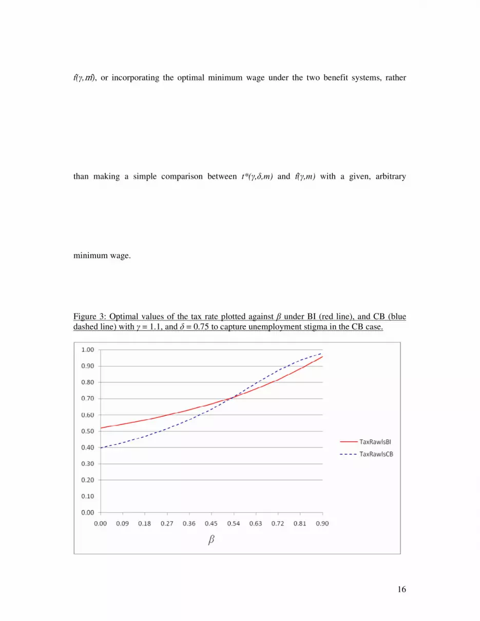
16

t �(�,��), or incorporating the optimal minimum wage under the two benefit systems, rather

than making a simple comparison between t*(�,�,m) and t�(�,m) with a given, arbitrary

minimum wage.

Figure 3: Optimal values of the tax rate plotted against � under BI (red line), and CB (blue dashed line) with � = 1.1, and � = 0.75 to capture unemployment stigma in the CB case.

17

Figures 4-7 are related. In Figure 4, optimal BI and CB for the Rawlsian case are

compared, over the usual range of � – showing that CB is higher throughout.

Figure 4: Optimally chosen BI and CB (vertical axis) against �, Rawlsian case.

Figure 5 makes a similar comparison for the utilitarian objective and finds that the plots in

this case cross twice, so that optimal BI is higher for mid-range values of �. Again this is far

from obvious, and the ‘inefficiency’ of the CB, which delivers less well-being in spite of its

greater magnitude over most of the range of relativity, is also noteworthy (see also Figure

10).

18

Figure 5: Optimally chosen BI and categorical benefit (vertical axis) against � (horizontal axis), utilitarian case.

Figure 6 shows how optimally-chosen BI varies as � increases, for our two objectives.

When � = 0, so that relative income is irrelevant, the Rawlsian objective gives a higher

optimal BI than the utilitarian (by 19%), as expected. As � is increased, the optimal BI

initially rises in both cases. However, the rise is – rather surprisingly – steeper for the

19

utilitarian case, so the two lines cross at about � = 0.27. In both cases, optimal BI peaks4 in

the range [0.45,0.54] for �. Furthermore, optimal BI under both objectives then declines with

still higher concern, converging to the same low level for � = 0.9. Intuitively, there are two

opposing effects of the increasing externality from higher concern for relativity. Initially a

higher tax reduces socially excessive labour supply, generating greater BI and higher

unemployment, but for large � the shrinking tax base and revenues (shown below) combine

to yield lower optimal BI.

Figure 6: Optimally chosen BI (vertical axis) against � (horizontal axis).

Figure 7 shows how the optimally chosen CB varies with �. When � = 0, so that

relative income is irrelevant, the Rawlsian case gives a higher optimal CB than the utilitarian

case (this result parallels our earlier finding for BI). As � is increased, the optimal benefit

initially rises in both cases. However, the rise is a little steeper for the utilitarian case, so the

4 Figure 6 reveals variations in optimal BI over � which are quite substantial though non-monotonic.

20

two lines cross at about � = 0.45. Optimal CB peaks5 around � = 0.54 in the Rawlsian case,

but closer to � = 0.72 under a utilitarian approach, and then again declines.

Figure 7: Optimally chosen CB (vertical axis) against � (horizontal axis).

Figure 8 shows how all the optimal tax rates increase with � as expected, essentially

to offset the increasing externality imposed by own earnings on others as concern for

relativity rises. Equally intuitively, optimal tax with BI is generally greater than optimal tax

with CB, whatever the social objective. Most interestingly, however, optimal Rawlsian and

5 Figure 7 shows variations in optimal CB over � which are less substantial than those for optimal BI.

21

utilitarian taxes converge for high �, (remaining higher for BI than for CB). Intuitively, the

growing weight of the externality in individual utility comes to dominate the differing social

objectives, for high enough concern for relativity. However the high taxes for high � are

rather implausible, suggesting that the middle of the range is more realistic.

As will be indicated in Figures 10-12, the behaviour of the optimal effective minimum

wage (and corresponding non-employment) – as � is increased from zero – parallel that of the

optimal tax rate, by rising with increasing concern for relative income and by being higher in

the Rawlsian case than the utilitarian case6. However, the optimal effective minimum wage

and non-employment are both lower for a BI system than for a CB, as expected.

Figure 8: Optimally chosen tax rate (vertical axis) against � (horizontal axis).

Figure 9 demonstrates how total (optimal) tax revenue, and hence ‘size of

government’ varies with �. In terms of the public finances, we expect an optimal BI system to

6 Again (for both the minimum wage and the unemployment rate), this gap diminishes as � rises under a basic income; but not under a categorical benefit until mid-range values of � are reached.

22

be more expensive than a corresponding CB system. Though more tax revenue must be

collected under a Rawlsian (rather than utilitarian) objective7 when relative income is

unimportant, this inequality reverses – as soon as � reaches about 0.3 in the case of a BI, but

only when � approaches 0.7 for a CB.

Figure 9: Tax revenue under optimal tax rate (vertical axis) against � (horizontal axis).

Figure 10 considers the utilitarian objective. We show how aggregate utility varies

with the effective minimum wage, m, for three chosen values of � – zero (no concern for

relative income), 0.45 (intermediate) and 0.9 (very high). For each value of �, we consider

both BI and CB. Under BI, the optimal effective minimum wage (and thus the unemployment

rate) increases with concern for relative income. With CB the initially fairly flat utility plot

7 A higher effective minimum wage and higher tax rate both tend to reduce mean income, outweighing the opposite effect of a lower employment rate. In spite of also having lower employment to tax, the higher Rawlsian tax rate is initially sufficient to allow more tax revenue to be collected than in the utilitarian case.

23

means that an optimal minimum wage is difficult to identify, which is why we do not follow

the presentation of the Rawlsian results in Figure 1. There are several interesting conclusions

from Figure 10. With no concern for relativity, BI and CB yield approximately optimal and

equal utilitarian welfare over an initial range of (low) minimum wages, though BI-well-being

then falls rapidly below CB-well-being as m rises. For realistic intermediate (and also high) �,

BI dominates CB by an increasingly wide margin. With BI, optimal unemployment is much

lower than with CB (although the gap narrows for high �).

Figure 10: Utilitarian utility plotted against m, for three values of �, under BI (1) and CB (2).

This yields a tentative possible explanation for the view that BI is not an efficient

transfer system. With traditional neglect of concern for relativity in policy making, and a

‘political’ minimum wage above the equivalent of 0.2 in Figure 10, the steep decline of BI

welfare for perceived � = 0 appears to support CB. Yet with realistic concern for relativity,

the welfare comparison is dramatically reversed.

(1) β = 0.00

(2) β = 0.00

(1) β = 0.45

(2) β = 0.45

(1) β = 0.90

(2) β = 0.90

24

For good reasons, we have concentrated so far on measures of social welfare, and the

corresponding values taken by the minimum wage, unemployment, tax rate and the

government budget. However, underlying this is a heterogeneous population of potential

workers. Figures 11 and 12 offer some illustration of which individuals (within the ability

distribution) tend to benefit more under the various policies and preferences we have

considered. A black vertical line in each figure shows the halfway point in the population – at

a wage level of just above 0.3, because of the negative skewness of the wage distribution. In

Figure 11, Rawlsian policy leaves unemployed individuals (shown by the horizontal sections

on the left) slightly better off under CB than BI when relative income is considered irrelevant.

However, a CB leaves more individuals (over half of the population) without a job – such

that the highest ability unemployed and the lowest paid working poor are better off with BI,

when more people would work. Nonetheless, Figure 11 also shows that high ability

individuals prefer the CB system because of the lower tax when � = 0. However, when

relative income has even moderate importance (� = 0.36), all individuals prefer the BI

system, regardless of their ability.

Figure 11: Individual utility (vertical axis) against wage rate or implied ability (horizontal axis) in the Rawlsian case.

25

Figure 12 displays very similar results under a utilitarian social objective, while also

showing higher employment rates (compared to each counterpart from Figure 11).

Remarkably, well-being of the unemployed is almost the same under Rawlsian and utilitarian

BI, and substantially lower in each case with CB. Furthermore, when � = 0, more mid-range

ability individuals prefer the BI system over CB than with a Rawlsian objective. Clearly,

there will be an intermediate value of � above which a majority of the population will prefer

BI, for each objective.

Figure 12: Individual utility (vertical axis) against wage rate or implied ability (horizontal axis) in the utilitarian case.

26

As noted in Section 2, optimal individual effort under a BI increases with concern for

relative income (�) for a given effective minimum wage (m) and wage (w), and also rises

with w. Figure 13 shows how optimal effort, now using optimal m, increases with the wage –

in the Rawlsian case with BI. Lower unemployment evident in Figure 11 for � = 0 is reflected

in positive optimal effort at a lower wage than when � = 0.36. At wages up to about 0.5

(more than half of the population, given the skewness of the wage distribution), optimal effort

is higher for lower �, (with the optimal minimum wage). This is a surprising result, because

we have seen that, for given m, optimal effort rises with � , so it due to the offsetting effect of

the increasing optimal minimum wage. The two upper plots with CB show greater

unemployment than with BI, and higher effort for all workers with higher �, as expected.

Under the lower CB tax (Fig.2), effort is always higher than corresponding BI effort.

Figure 13: Optimal values of effort (with optimal m) plotted against w for the Rawlsian case under a BI for � = 0 and � = 0.36.

27

Following equation (11), we also noted that equilibrium mean income under a BI also

increases with �, again for given m. Figure 14, below, demonstrates that – if the optimal

minimum wage is used – mean income under a BI initially rises slightly with �, but then falls

back for moderate and high concern for relativity as tax continues to rise. Further, mean

income under a CB (with a similar path) is much higher than with BI, for any given �. This

difference is enhanced by there being fewer low earners and more unemployment. The higher

comparator income with CB also reduces well-being for all compared to BI, as shown in

earlier Figures.

Figure 14: Optimal mean income (vertical axis) plotted against � (horizontal axis) for BI (red line), and CB (blue dashed line), � = 1.5.

28

5. Conclusions

We have constructed a model which allows basic income (BI) and categorical benefit

(CB) to be compared in a simple general equilibrium model – combining worker

heterogeneity, extensive and intensive margins of labour supply, as well as including concern

for relative income, and declining marginal utility of own consumption. Our simulations

compare Rawlsian and utilitarian policy under these two fundamentally different systems of

redistribution, yielding interesting and surprising results that could not be derived

analytically. A major surprise is that modest concern for relativity implies Pareto dominance

of BI, (in spite of associated higher tax), when compared to CB (with higher unemployment,

and effort by the employed), under both Rawlsian and utilitarian goals. Another surprise

under moderate relativity concern is that the two radically different policy objectives provide

essentially the same utility to the non-employed, though high earners benefit from the lower

29

utilitarian tax. (In the traditional case of no concern for relativity, the rich and most

unemployed do prefer CB). While the levels of optimal BI and CB initially rise with concern

for relativity, they then decline, though optimal unemployment, taxes and minimum wages all

increase monotonically, with higher tax and lower individual effort and unemployment under

BI as expected. While optimal unemployment levels appear high, they can be interpreted as

‘non-employment’ in a total population which includes individuals with arbitrarily low

productivities who would not normally be included in the labour force.

These simulations have not generally included the realistic stigma or utility loss from

unemployment under CB, which was included in our model. This would clearly enhance the

relative advantage of BI, and we presented one example with stigma where the optimal

Rawlsian tax becomes higher with CB than for BI when concern for relativity is important.

Overall, we have found a remarkable dominance of BI when relative income is

important for individual well-being, as well as much less difference in the outcomes of

Rawlsian and utilitarian policies than expected. Many important aspects of BI, and

determinants of SWB, that have been discussed in the literature are neglected here, and

should be included in future research on these important issues.

References

A.B. Atkinson (1995). Public Economics in Action: The Basic Income/Flat Tax Proposal. Oxford: Oxford University Press. J. A. Beath & FitzRoy, F.R. (2009). “Public economics of relative income and subjective well-being”, paper presented at the SIRE-Cornell Conference on Relativity, Inequality and Public Policy, Edinburgh, 2009. M.J. Boskin & Sheshinski, E. (1978). “Optimal redistributive taxation when individual welfare depends upon relative income”. Quarterly Journal of Economics, 92(4), pp. 589-601. A.E. Clark, E.P. Frijters & Shields, M.A. (2008). “Relative income, happiness, and utility: An explanation for the Easterlin paradox and other puzzles”, Journal of Economic Literature, 46(1): pp. 95-144. U. Colombino, M. Locatelli, E. Narazani & O’Donoghue, C. (2010). “Alternative basic income mechanisms: An evaluation exercise with a microeconometric model”. IZA DP No. 4781, Bonn.

30

R. Easterlin (1974). “Does Economic Growth Improve the Human Lot?” in P.A. David and M.W. Reder, eds., Nations and Households in Economic Growth: Essays in Honour of Moses Abramowitz. New York: Academic Press, pp. 89-125. R. Easterlin & Angelescu, L. (2009). “Happiness and Growth the World Over: Time Series Evidence on the Happiness-Income Paradox”, IZA Discussion Paper No. 4060, Available at http://ftp.iza.org/dp4060.pdf. C. B. Eaton &. Eswaran M. (2009), “Well-being and Affluence in the Presence of a Veblen Good”, The Economic Journal, 119, pp. 1088-1104. M. Evers, R. De Mooij and Van Vuuren, D. (2008). “The wage elasticity of labour supply: a synthesis of empirical estimates”. De Economist, 156(1), pp. 25-43. F. R. FitzRoy and Jin, J. (2010). “Efficient redistribution: Comparing basic income and unemployment benefit”, ms, School of Economics and Finance, University of St. Andrews. B.S. Frey (2008). Happiness. A Revolution in Economics. Cambridge, MA: MIT Press. H. Immervoll, H. Kleven, C. Kriener, & Saez, E. (2007). “Welfare reform in European countries: A microsimulation analysis”. Economic Journal, 117, no. 516, pp. 1-44. R. Kanbur & Tuomala, M. (2009). “Relativity, inequality, and optimal non-linear income taxation”, paper presented at the SIRE-Cornell Conference on Relativity, Inequality and Public Policy, Edinburgh, 2009. L. Kaplow (2008). The Theory of Taxation and Public Economics, Princeton University Press, Princeton and Oxford. R. Layard (1980). “Human satisfactions and public policy”, Economic Journal, 90, 737-750. R. Layard (2005). Happiness, Lessons from a New Science, Allen Lane, London.

R. Layard (2006). “Happiness and Public Policy: A challenge to the Profession”, Economic Journal, 116, C24 – C33. R. Layard (2009). “The Greatest Happiness Principle: Its time has come”, Well-being: How to lead the good life and what government should do to help, (eds) S Griffiths and R Reeves, Social Market Foundation, July 2009. R. Layard, G. Mayraz & Nickell, S. (2010). “Does Relative Income Matter? Are the Critics Right?” Chapter 6 in E. Diener, J. F. Helliwell and D. Kahneman, eds., International Differences in Well-being, Oxford University Press. N.G. Mankiw, M. Weinzierl & Yagan, D. (2009). “Optimal taxation in Theory and Practice”, NBER Working Paper No. 15071. A. Oswald, (2009). “Emotional Prosperity”, BJIR Annual Lecture at the London School of Economics, November 2009. A. Oswald (1983). “Altruism, jealousy and the theory of optimal non-linear taxation”, Journal of Public Economics, 20, pp. 77–87. A. Oswald, & Wu, S. (2010). “Objective Confirmation of Subjective Measures of Human Well-being: Evidence from the USA”, Science, February 2010. J.E. Stiglitz, A. Sen & Fitoussi, J.P. (2010). Mismeasuring our Lives: Why GDP Doesn’t Add Up. New Press, New York, NY.