Relaxation of certain integral functionals arising in imaging

models

Ana Margarida Ribeiro∗, Elvira Zappale†

February 1, 2011

Abstract

We provide a relaxation result in BV × Lq, 1 ≤ q < +∞ for integral decoupled energies arisingin image analysis, in the spirit of the total variation decomposition models.Keywords: Relaxation, functions of bounded variation, quasiconvexity, image decomposition.MSC2010 classification: 49J45, 74F99.

1 Introduction

Recently new concepts and new targets entered in image analysis for decomposition and restoration:decompose in the RGB model a given image φ : Ω → R3 (Ω ⊂ R2) into two components u and v, suchthat φ = u + v where u is a ’cartoon’ representation of φ , a simplified approximation describing thethree colors decomposition, while v is the oscillatory component, consisting of ’texture’ or ’noise’. Thisnew image analysis task has been first formulated in theory by Meyer [19] and the approach, classicallyadopted in literature (see [20], [22]) is a total variation minimization model first proposed in [21], coupledwith the presence of an oscillatory function.

To capture the characteristics of each part in which the given image φ is decomposed, the u component,representing a ‘cartoon’ of the image φ is modeled by a function of bounded variation, while the vcomponent representing ’texture’ or ‘noise’ is modeled by an oscillatory function, bounded in some norm,suitable for numerical purposes. Often v is assumed to be an L2 function.

In particular, in [19] the following minimization problem has been formulated

inf(u, v) ∈ BV ×G s.t. φ = u+ v

|Du|(Ω) + ‖v‖G (1.1)

where G denotes some suitable Banach space, in fact many choices for the space G have been successfullyconsidered by Osher, Sole and Vese (see [20], [22], [23]). A different approach has been considered in [4],[5], and [6] i.e.

infu∈BV,‖v‖G≤µ

|Du|(Ω) +

1

2λ‖φ− u− v‖2L2

(1.2)

where µ represents a bound for the norm of v and λ a scaling factor for the L2 norm of the fidelity termφ− (u+ v).

Our note is devoted to generalize the above mentioned decomposition models, by considering a for-mulation more general than (1.1) and (1.2), replacing the total variation term |Du|(Ω) by the integral∫

Ω

W (∇u(x)) dx, with W not necessarily convex, and u ∈W 1,1(Ω;R3). To this term we add the integral∫Ω

ϕ(x, u(x), v(x)) dx which may recover the fidelity term ‖φ− u− v‖2L2 . Considering also more general

∗Departamento de Matematica and CMA, Faculdade de Ciencias e Tecnologia - Universidade Nova de Lisboa, Quintada Torre, 2829-516 Caparica, Portugal. E-mail: amfr@fct.unl.pt†D.I.E.I.I, Universita’ degli Studi di Salerno, Via Ponte Don Melillo, 84084 Fisciano (SA) Italy. E-mail:ezappale@unisa.it

1

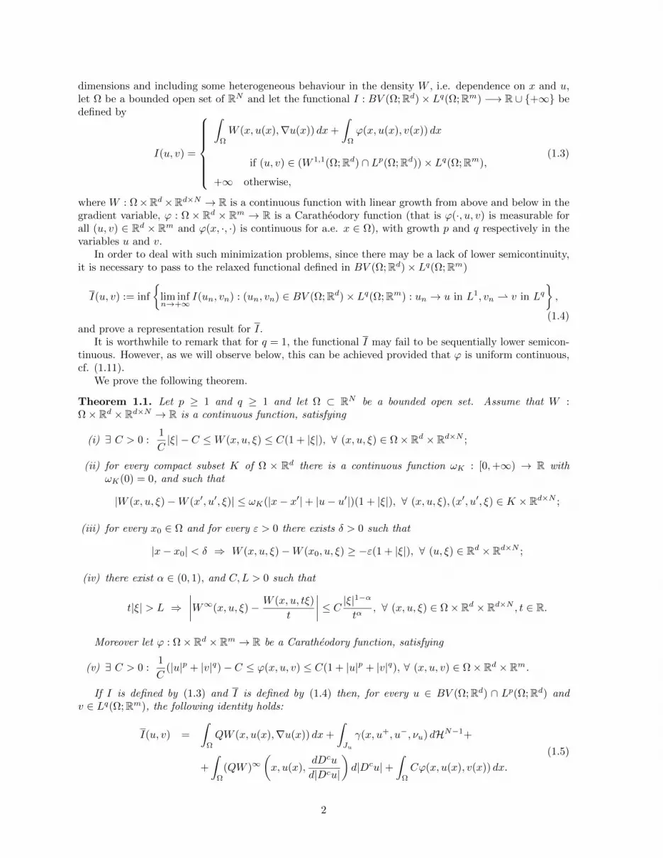
dimensions and including some heterogeneous behaviour in the density W , i.e. dependence on x and u,let Ω be a bounded open set of RN and let the functional I : BV (Ω;Rd)× Lq(Ω;Rm) −→ R ∪ +∞ bedefined by

I(u, v) =

∫Ω

W (x, u(x),∇u(x)) dx+

∫Ω

ϕ(x, u(x), v(x)) dx

if (u, v) ∈ (W 1,1(Ω;Rd) ∩ Lp(Ω;Rd))× Lq(Ω;Rm),

+∞ otherwise,

(1.3)

where W : Ω×Rd×Rd×N → R is a continuous function with linear growth from above and below in thegradient variable, ϕ : Ω × Rd × Rm → R is a Caratheodory function (that is ϕ(·, u, v) is measurable forall (u, v) ∈ Rd × Rm and ϕ(x, ·, ·) is continuous for a.e. x ∈ Ω), with growth p and q respectively in thevariables u and v.

In order to deal with such minimization problems, since there may be a lack of lower semicontinuity,it is necessary to pass to the relaxed functional defined in BV (Ω;Rd)× Lq(Ω;Rm)

I(u, v) := inf

lim infn→+∞

I(un, vn) : (un, vn) ∈ BV (Ω;Rd)× Lq(Ω;Rm) : un → u in L1, vn v in Lq,

(1.4)and prove a representation result for I.

It is worthwhile to remark that for q = 1, the functional I may fail to be sequentially lower semicon-tinuous. However, as we will observe below, this can be achieved provided that ϕ is uniform continuous,cf. (1.11).

We prove the following theorem.

Theorem 1.1. Let p ≥ 1 and q ≥ 1 and let Ω ⊂ RN be a bounded open set. Assume that W :Ω× Rd × Rd×N → R is a continuous function, satisfying

(i) ∃ C > 0 :1

C|ξ| − C ≤W (x, u, ξ) ≤ C(1 + |ξ|), ∀ (x, u, ξ) ∈ Ω× Rd × Rd×N ;

(ii) for every compact subset K of Ω × Rd there is a continuous function ωK : [0,+∞) → R withωK(0) = 0, and such that

|W (x, u, ξ)−W (x′, u′, ξ)| ≤ ωK(|x− x′|+ |u− u′|)(1 + |ξ|), ∀ (x, u, ξ), (x′, u′, ξ) ∈ K × Rd×N ;

(iii) for every x0 ∈ Ω and for every ε > 0 there exists δ > 0 such that

|x− x0| < δ ⇒ W (x, u, ξ)−W (x0, u, ξ) ≥ −ε(1 + |ξ|), ∀ (u, ξ) ∈ Rd × Rd×N ;

(iv) there exist α ∈ (0, 1), and C,L > 0 such that

t|ξ| > L ⇒∣∣∣∣W∞(x, u, ξ)− W (x, u, tξ)

t

∣∣∣∣ ≤ C |ξ|1−αtα, ∀ (x, u, ξ) ∈ Ω× Rd × Rd×N , t ∈ R.

Moreover let ϕ : Ω× Rd × Rm → R be a Caratheodory function, satisfying

(v) ∃ C > 0 :1

C(|u|p + |v|q)− C ≤ ϕ(x, u, v) ≤ C(1 + |u|p + |v|q), ∀ (x, u, v) ∈ Ω× Rd × Rm.

If I is defined by (1.3) and I is defined by (1.4) then, for every u ∈ BV (Ω;Rd) ∩ Lp(Ω;Rd) andv ∈ Lq(Ω;Rm), the following identity holds:

I(u, v) =

∫Ω

QW (x, u(x),∇u(x)) dx+

∫Ju

γ(x, u+, u−, νu) dHN−1+

+

∫Ω

(QW )∞(x, u(x),

dDcu

d|Dcu|

)d|Dcu|+

∫Ω

Cϕ(x, u(x), v(x)) dx.

(1.5)

2

We also observe that the above result can be recasted also in the framework of relaxation resultsdealing with integral functionals arising in Nonlinear Elasticity for materials whose behaviour dependson the strain and on the chemical composition, cf. [14, 15].

In order to describe the right hand side of (1.5) we recall that for every x ∈ Ω, QW (x, u, ·) standsfor the quasiconvexification of W , cf. (2.1), while (QW )∞ denotes the recession function of QW withrespect to the last variable as introduced in Definition 2.4, and γ stands for the surface integral density,defined in (2.8). Finally for every (x, u) ∈ Ω×Rd, Cϕ stands for the convex envelope (or convexification)of ϕ(x, u, ·), namely

Cϕ(x, u, ·) := supg : Rm → R : g convex, g(v) ≤ ϕ(x, u, v) ∀ v. (1.6)

Classical results in Calculus of Variations ensure that, if ϕ takes only finite values then Cϕ coincideswith the bidual of ϕ, ϕ∗∗, whose characterization is given below

ϕ∗∗(x, u, ·) := supg : Rm → R : g convex and lower semicontinuous, g(v) ≤ ϕ(x, u, v) ∀ v. (1.7)

Remark 1.2.

• We observe that in the Sobolev setting, Theorem 1.1 can be proven without coercivity assumptionson ϕ, indeed let f : Ω× Rd × Rd×N × Rm → R be a Caratheodory function satisfying

0 ≤ f (x, u, ξ, v) ≤ C (1 + |u|p + |ξ|p + |v|q)

for a.e. x ∈ Ω, for every (u, ξ, v) ∈ Rd × Rd×N × Rm and for some C > 0. Consider for every1 ≤ p, q < +∞ the following relaxed localized energy

F (u, v;A) :=

inf

lim infn→∞

∫A

f (x, un (x) ,∇un (x) , vn (x)) dx : un u in W 1,p(A;Rd

), vn v in Lq (A;Rm)

.

(1.8)Then, in [10, Theorem 1.1](cf. also [9]) it has been proven that, for every u ∈ W 1,p

(Ω;Rd

),

v ∈ Lq (Ω;Rm) and A ∈ A (Ω) ,

F (u, v;A) =

∫A

QCf (x, u (x) ,∇u (x) , v (x)) dx,

where QCf stands for the quasiconvex-convex envelope of f with respect to the last two variables,namely

QCf(x, u, ξ, v) =

inf

1

|D|

∫D

f(x, u, ξ +∇ϕ(y), v + η(y)) dy : ϕ ∈W 1,∞0 (D;Rd), η ∈ L∞(D;Rm),

∫D

η(y) dy = 0

,

(1.9)D being any bounded open set. Clearly this equality recovers our setting, since it suffices to definefor every (x, u, ξ, v) ∈ Ω × Rd × Rd×N × Rm, f(x, u, ξ, v) := W (x, u, ξ) + ϕ(x, u, v). In fact it iseasily seen that if f satisfies the above growth assumptions, then

QCf(x, u, ξ, v) = QW (x, u, ξ) + Cϕ(x, u, v).

• We emphasize that the arguments adopted to prove the previous theorem strongly rely on the factthat the energy densities are decoupled. In particular, in the case q = 1, we will approximate the

3

functional I by adding an extra term with superlinear growth at ∞ in the v variable. This willensure the sequentially weak lower semicontinuity of the relaxed approximating functional

Iε(u, v) := inf

lim inf

n

∫Ω

W (x, un,∇un) dx+

∫Ω

(ϕ(x, u, v) + εθ(|v|)) dx :

un → u in L1, vn v in L1,

allowing us to adopt arguments similar to those exploited in the proof for the case q > 1. Thesetechniques are well suited for the convex setting but we are not aware if a similar procedure ispossible in the quasiconvex-convex framework.

Having in mind the continuous embedding of BV (Ω;Rd) in LNN−1 (Ω;Rd) (assuming Ω ⊂ RN ), we can

obtain, in an easier way, the relaxation result as above. Indeed we can prove the following result.

Theorem 1.3. Let Ω ⊂ RN be a bounded open set, and let 1 ≤ p ≤ NN−1 and q ≥ 1. Let W : Ω× Rd ×

Rd×N → R be a continuous function satisfying (i)÷(iv) of Theorem 1.1. Moreover let ϕ : Ω×Rd×Rm → Rbe a Caratheodory function satisfying (v) of Theorem 1.1 in the weaker form

∃ C > 0 :1

C|v|q − C ≤ ϕ(x, u, v) ≤ C(1 + |u|p + |v|q), ∀ (x, u, v) ∈ Ω× Rd × Rm. (1.10)

Then, for every (u, v) ∈ BV (Ω;Rd)× Lq(Ω;Rm), (1.5) holds.

Remark 1.4. The continuous embedding of BV (Ω;Rd) into LNN−1 (Ω;Rd) (with Ω ⊂ RN ) allows us to

have the just established result, also replacing (1.10) by the following condition:

∃ C > 0 :1

C|v|q − C ≤ ϕ(x, u, v) ≤ C(1 + |u|r + |v|q), ∀ (x, u, v) ∈ Ω× Rd × Rm

and for some r ∈[1, N

N−1

].

We observe that under assumptions (i) ÷ (iv) of Theorem 1.1, [17, Theorem 2.16] ensures that thefunctional∫

Ω

QW (x, u,∇u) dx+

∫Ju

γ(x, u+, u−, νu) dHN−1 +

∫Ω

(QW )∞(x, u,

dDcu

d|Dcu|

)d|Dcu|

is lower semicontinuous with respect to the strong-L1 topology. Moreover [16, Theorem 7.5] guaranteesthat ∫

Ω

Cϕ(x, u, v) dx

is sequentially weakly lower semicontinuous with respect to L1strong×L1

weak-topology provided the functionCϕ is convex in the last variable, satisfies suitable growth conditions, as those in (2.5) and (2.6), andthat the function Cϕ(x, ·, ·) is lower semicontinuous. We will observe in Remark 2.3 below that this lattercondition may not be verified just under the assumptions of Theorems 1.1 and 1.3. On the other hand anargument entirely similar to [11, Theorem 9.5] guarantees that Cϕ(x, ·, ·) is lower semicontinuous (evencontinuous) by assuming additionally that

|ϕ(x, u, ξ)− ϕ(x, u′, ξ)| ≤ ω′(|u− u′|)(|ξ|+ 1) (1.11)

for a suitable modulus of continuity ω′, i.e. ω′ : R+∪0 → R+∪0 continuous and such that ω′(0) = 0.Consequently the superadditivity of lim inf entails the sequentially strong-weak lower semicontinuity

of the right hand side of (1.5) even for q = 1.

4

2 Notations and General Facts

2.1 Properties of the integral density functions

In this subsection we recall several notions applied to functions like quasiconvexity, envelopes and recessionfunction, etc. We also recall or prove properties of those functions that will be useful through the paper.Such notions and related properties will apply to the density functions that will appear in the relaxedfunctionals that we characterize. We start recalling the notion of quasiconvex function due to Morrey.

Definition 2.1. A Borel measurable function h : Rd×N → R is said to be quasiconvex if there exists abounded open set D of RN such that

h(ξ) ≤ 1

|D|

∫D

h(ξ +∇ϕ(x)) dx,

for every ξ ∈ Rd×N , and for every ϕ ∈W 1,∞0 (D;Rd).

If h : Rd×N → R is any given Borel measurable function bounded from below, it can be defined thequasiconvex envelope of h, that is the largest quasiconvex function below h:

Qh(ξ) := supg(ξ) : g ≤ h, g quasiconvex.

Moreover, as well known (see the monograph [11]),

Qh(ξ) := inf

1

|D|

∫D

h(ξ +∇ϕ(x)) dx : ϕ ∈W 1,∞0 (D;Rd)

, (2.1)

for any bounded open set D ⊂ RN .

Proposition 2.2. Let Ω ⊂ RN be a bounded open set and

W : Ω× Rd × Rd×N → [0,+∞)

be a continuous function. Let QW be the quasiconvexification of W (see (2.1)). Then the validity of (i)in Theorem 1.1 guarantees that there exists a constant C > 0 such that

1

C|ξ| − C ≤ QW (x, u, ξ) ≤ C(1 + |ξ|), ∀ (x, u, ξ) ∈ Ω× Rd × Rd×N . (2.2)

The validity of (i) and (ii) of Theorem 1.1 ensures that for every compact set K ⊂ Ω × Rd, thereexists a continuous function ω′K : R→ [0,+∞) such that ω′K(0) = 0 and

|QW (x, u, ξ)−QW (x′, u′, ξ)| ≤ ω′K(|x−x′|+ |u−u′|)(1 + |ξ|), ∀ (x, u), (x′, u′) ∈ K, ∀ ξ ∈ Rd×N . (2.3)

Conditions (i) and (iii) of Theorem 1.1 entail that, for every x0 ∈ Ω and ε > 0, there exists δ > 0such that

|x− x0| ≤ δ ⇒ ∀ (u, ξ) ∈ Rd × Rd×N QW (x, u, ξ)−QW (x0, u, ξ) ≥ −ε(1 + |ξ|). (2.4)

Moreover, if W satisfies conditions (i) and (ii) of Theorem 1.1, QW is a continuous function.

Remark 2.3. Analogous arguments entail that, under hypothesis (v) of Theorems 1.1 and 1.3, respec-tively,

∃C > 0 :1

C(|u|p + |v|q)− C ≤ Cϕ(x, u, v) ≤ C(1 + |u|p + |v|q), ∀ (x, u, v) ∈ Ω× Rd × Rm, (2.5)

and

∃C > 0 :1

C|v|q − C ≤ Cϕ(x, u, v) ≤ C(1 + |u|p + |v|q), ∀ (x, u, v) ∈ Ω× Rd × Rm. (2.6)

On the other hand we emphasize that being ϕ as in Theorems 1.1 and 1.3, namely a Caratheodoryfunction, this is not enough to guarantee that Cϕ is still a Caratheodory function, cf. Example 9.6 in [11]and Example 7.14 in [16]. In particular Cϕ turns out to be measurable in x, upper semicontinuous in u,convex and hence continuous in ξ. Furthermore if q > 1, [12, Lemma 4.3] guarantees that Cϕ(x, ·, ·) islower semicontinuous.

5

Proof. By definition of the quasiconvex envelope of W , it is easily seen that (i) of Theorem 1.1 entails(2.2) with the same constant appearing in (i).

Next we prove (2.3). Let K be a compact set in Ω×Rd and take (x, u), (x′, u′) ∈ K. Let ε > 0, thenusing condition (2.1), we find ϕε ∈W 1,∞

0 (Q;Rd), Q being the unitary cube, such that

QW (x, u, ξ) ≥ −ε+

∫Q

W (x, u, ξ +∇ϕε(y)) dy.

Now, we observe that, by virtue of the coercivity condition expressed by (i) of Theorem 1.1 and by (2.2),it follows that

‖ξ +∇ϕε‖L1 ≤ c(1 + |ξ|).

By condition (ii) of Theorem 1.1, for every (x, u), (x′, u′) ∈ K and for every ξ ∈ Rd×N , it results

|W (x, u, ξ)−W (x′, u′, ξ)| ≤ ωK(|x− x′|+ |u− u′|)(1 + |ξ|).

Then we can write the following chain of inequalities:

QW (x, u, ξ) ≥ −ε+

∫Q

W (x, u, ξ +∇ϕε(y)) dy

≥ −ε−∫Q

λ(y) dy +

∫Q

W (x′, u′, ξ +∇ϕε(y)) dy,

where λ(y) := |W (x, u, ξ + ∇ϕε(y)) −W (x′, u′, ξ + ∇ϕε(y))|. We therefore get, from the definition ofQW (x′, u′, ξ), that,

QW (x′, u′, ξ)−QW (x, u, ξ) ≤ ε+ ωK(|x− x′|+ |u− u′|)(1 + ‖ξ +∇ϕε‖L1)

≤ ε+ ωK(|x− x′|+ |u− u′|)(1 + c(1 + |ξ|)).

Since ε is arbitrarily chosen, and since we can obtain in a similar way the same inequality with x in theplace of x′, and u in the place of u′, we get (2.3).

In order to prove condition (2.4), we fix x0 ∈ Ω and ε > 0. As before, for every x ∈ Ω and for everyσ > 0, by (2.1), the coercivity condition expressed by (i) of Theorem 1.1, and by (2.2), there exist aconstant c > 0 and a function ϕσ ∈W 1,∞

0 (Q;Rd) such that

QW (x, u, ξ) ≥ −σ +

∫Q

W (x, u, ξ +∇ϕσ(y)) dy,

with ‖ξ +∇ϕσ‖L1 ≤ c(1 + |ξ|).Thus arguing as above, and exploiting condition (iii) of Theorem 1.1, we have the following chain of

inequalities, for |x− x0| < δ with δ as in condition (iii) of Theorem 1.1,

QW (x0, u, ξ) ≤∫Q

W (x0, u, ξ +∇ϕσ(y)) dy

≤∫Q

W (x, u, ξ +∇ϕσ(y)) dy + ε

∫Q

(1 + |ξ +∇ϕσ(y)|) dy

≤ QW (x, u, ξ) + σ + ε(1 + c(1 + |ξ|)).

Thus it suffices to let σ go to 0 in order to achieve the statement.Finally we prove the continuity of QW . We need to show that, for every ε > 0 and (x0, u0, ξ0) ∈

Ω× Rd × Rd×N , there is δ ≡ δ(ε, x0, u0, ξ0) > 0 such that

|x− x0|+ |u− u0|+ |ξ − ξ0| ≤ δ ⇒ |QW (x, u, ξ)−QW (x0, u0, ξ0)| ≤ ε. (2.7)

6

Let ε > 0 be fixed. Since QW is quasiconvex on ξ, QW (x0, u0, ·) is continuous and thus we can findδ1 = δ1(ε, x0, u0, ξ0) > 0 such that

|ξ − ξ0| ≤ δ1 ⇒ |QW (x0, u0, ξ)−QW (x0, u0, ξ0)| ≤ ε

2.

Moreover, by virtue of (2.3), defining K := Bσ(x0, u0) for some σ > 0 such that K ⊂ Ω× Rd, one has

|ξ − ξ0| ≤ δ1 ⇒ |QW (x, u, ξ)−QW (x0, u0, ξ)| ≤ ω′K(|x− x0|+ |u− u0|)(1 + |ξ0|+ δ1).

Since ω′K is continuous and ω′K(0) = 0, there is δ2 = δ2(ε,K, ξ0) > 0 such that

|x− x0|+ |u− u0| ≤ δ2 ⇒ ω′K(|x− x0|+ |u− u0|) ≤ε

2(1 + |ξ0|+ 1).

Consequently, by choosing δ as minδ1, δ2, the above inequalities, and the triangular inequality giveindeed (2.7).

We also recall the definition of the recession function.

Definition 2.4. Let h : Rd×N → [0,+∞). The recession function of h is denoted by h∞ : Rd×N →[0,+∞), and defined as

h∞(ξ) := lim supt→+∞

h(tξ)

t.

Remark 2.5. (i) Recall that the recession function is a positively one homogeneous function, that isg(tξ) = tg(ξ) for every t ≥ 0 and ξ ∈ Rd×N .(ii) Through this paper we will work with functions W : Ω × Rd × Rd×N → [0,+∞) and W∞ is therecession function with respect to the last variable:

W∞(x, u, ξ) := lim supt→+∞

W (x, u, tξ)

t.

We trivially observe that, if W satisfies the growth condition (i) in Theorem 1.1, then W∞ satisfies1C |ξ| ≤W

∞(x, u, ξ) ≤ C|ξ|.(iii) As showed in [17, Remark 2.2 (ii)], if a function h : Rd×N −→ [0,+∞) is quasiconvex and satisfiesthe growth condition h(ξ) ≤ c(1 + |ξ|), for some c > 0, then, its recession function is also quasiconvex.

We now describe the surface energy density γ appearing in the characterization of I. Let W :Ω × Rd × Rd×N → R. By the notation above (QW )∞ is the recession function of the quasiconvexenvelope of W . Then γ : Ω× Rn × Rn × SN−1 −→ R is defined by

γ(x, a, b, ν) = inf

∫Qν

(QW )∞(x, φ(y),∇φ(y)) dy : φ ∈ A(a, b, ν)

, (2.8)

whereQν is the unit cube centered at the origin with faces parallel to ν, ν1, . . . , νN−1, for some orthonormalbasis of RN , ν1, . . . , νN−1, ν, and where

A(a, b, ν) :=

φ ∈W 1,1(Qν ,Rd) : φ(y) = a if < y, ν >=

1

2, φ(y) = b if < y, ν >= −1

2,

φ is 1− periodic in the ν1, . . . , νN−1 directions .

We observe that the function γ is the same whether we consider in the set A(a, b, ν), W 1,1(Qν ,Rd)functions (like in [18] and [17]) or W 1,∞(Qν ,Rd) functions (like in [2, page 312]). Moreover, if W doesn’tdepend on u, W : Ω× Rd×N → R, then γ(x, a, b, ν) = (QW )∞(x, (a− b)⊗ ν) (see [2, page 313]).

Properties of the function (QW )∞ will be important to get the integral representation of the relaxedfunctionals under consideration. In particular, a proof entirely similar to [7, Proposition 3.4] ensures thatfor every (x, u, ξ) ∈ Ω× Rd × Rd×N , Q(W∞)(x, u, ξ) = (QW )∞(x, u, ξ).

7

Proposition 2.6. Let W : Ω × Rd × Rd×N → [0,+∞) be a continuous function satisfying (i) and (iv)of Theorem 1.1. Then

Q(W∞)(x, u, ξ) = (QW )∞(x, u, ξ) for every (x, u, ξ) ∈ Ω× Rd × Rd×N . (2.9)

Proof. The proof will be achieved by double inequality.By definition of the quasiconvex envelope and the recession function, one gets (QW )∞ ≤ W∞ and

thus Q(QW )∞ ≤ Q(W∞). Since the recession function of a quasiconvex one is still quasiconvex, underhypothesis (i) of Theorem 1.1 (cf. Remark 2.5 (iii)) it follows that (QW )∞ ≤ Q(W∞).

In order to prove the opposite inequality we start noticing that, since by (i), the function W is boundedfrom below, we can assume without loss of generality that W ≥ 0. Then fix (x, u, ξ) ∈ Ω × Rd × Rd×Nand, for every t > 1, take ϕt ∈W 1,∞

0 (Q;Rd) such that∫Q

W (x, u, tξ +∇ϕt(y)) dy ≤ QW (x, u, tξ) + 1. (2.10)

By (i) and (2.2) we have that∥∥∇( 1

tϕt)∥∥L1(Q)

≤ C for a constant independent of t but just on ξ.

Defining ψt = 1tϕt, one has ψt ∈W 1,∞

0 (Q;Rd) and thus

Q(W∞)(x, u, ξ) ≤∫Q

W∞(x, u, ξ +∇ψt(y)) dy.

Let L be the constant appearing in condition (iv) of Theorem 1.1, we split the cube Q in the sety ∈ Q : t|ξ +∇ψt(y)| ≤ L and its complement in Q. Then we apply condition (iv) and the growth ofW∞ observed in Remark 2.5 (ii) to get

Q(W∞)(x, u, ξ) ≤∫Q

(C|ξ +∇ψt|1−α

tα+W (x, u, tξ +∇ϕt(y))

t+ C

L

t

)dy.

Applying Holder inequality and (2.10), we get

Q(W∞)(x, u, ξ) ≤ C

tα

(∫Q

|ξ +∇ψt| dy)1−α

+QW (x, u, tξ) + 1

t+ C

L

t,

and the desired inequality follows by definition of (QW )∞ and using the fact that ∇ψt has bounded L1

norm, letting t go to +∞.

The property of (QW )∞ stated next ensures that QW together with (QW )∞ satisfy the analogouscondition to (iv) of Theorem 1.1. To this end we first observe, as emphasized in [17], that (iv) in Theorem1.1 is equivalent to say that there exist C > 0 and α ∈ (0, 1) such that

|W∞(x, u, ξ)−W (x, u, ξ)| ≤ C(1 + |ξ|1−α) (2.11)

for every (x, u, ξ) ∈ Ω× Rd × Rd×N . Precisely we have the following result.

Proposition 2.7. Let W : Ω × Rd × Rd×N → [0,+∞) be a continuous function satisfying (i) and (iv)of Theorem 1.1. Then, there exist α ∈ (0, 1), and C ′ > 0 such that

|(QW )∞(x, u, ξ)−QW (x, u, ξ)| ≤ C(1 + |ξ|1−α), ∀ (x, u, ξ) ∈ Ω× Rd × Rd×N .

Proof. The thesis will be achieved by double inequality. Let α ∈ (0, 1) be as in (iv) of Theorem 1.1, seealso (2.11). Let ξ ∈ Rd×N , let Q be the unit cube in RN and let c be a positive constant varying fromline to line. For every ε > 0 by (2.1), find ϕ ∈W 1,∞

0 (Q;Rd) such that

QW (x, u, ξ) >

∫Q

W (x, u, ξ +∇ϕ(y)) dy − ε.

8

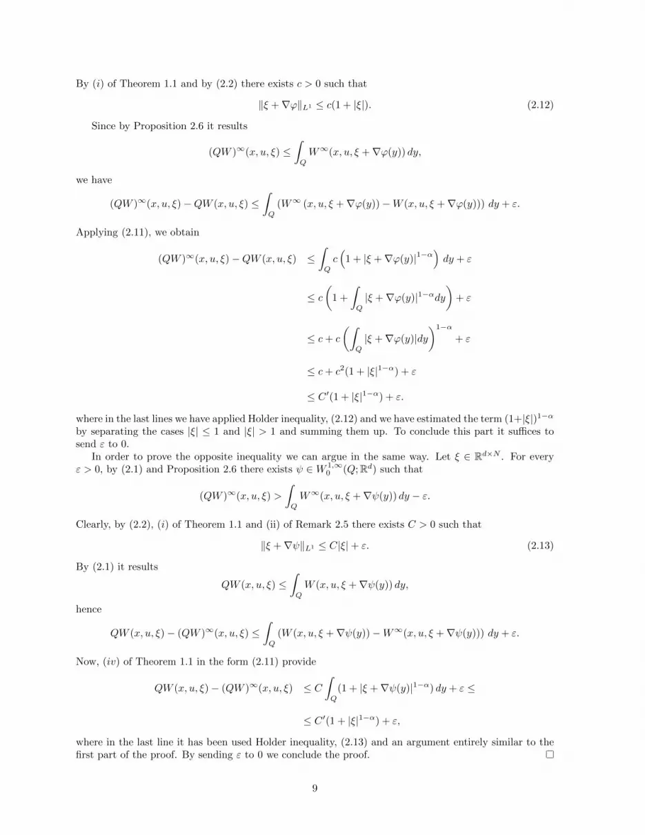
By (i) of Theorem 1.1 and by (2.2) there exists c > 0 such that

‖ξ +∇ϕ‖L1 ≤ c(1 + |ξ|). (2.12)

Since by Proposition 2.6 it results

(QW )∞(x, u, ξ) ≤∫Q

W∞(x, u, ξ +∇ϕ(y)) dy,

we have

(QW )∞(x, u, ξ)−QW (x, u, ξ) ≤∫Q

(W∞ (x, u, ξ +∇ϕ(y))−W (x, u, ξ +∇ϕ(y))) dy + ε.

Applying (2.11), we obtain

(QW )∞(x, u, ξ)−QW (x, u, ξ) ≤∫Q

c(

1 + |ξ +∇ϕ(y)|1−α)dy + ε

≤ c(

1 +

∫Q

|ξ +∇ϕ(y)|1−αdy)

+ ε

≤ c+ c

(∫Q

|ξ +∇ϕ(y)|dy)1−α

+ ε

≤ c+ c2(1 + |ξ|1−α) + ε

≤ C ′(1 + |ξ|1−α) + ε.

where in the last lines we have applied Holder inequality, (2.12) and we have estimated the term (1+|ξ|)1−α

by separating the cases |ξ| ≤ 1 and |ξ| > 1 and summing them up. To conclude this part it suffices tosend ε to 0.

In order to prove the opposite inequality we can argue in the same way. Let ξ ∈ Rd×N . For everyε > 0, by (2.1) and Proposition 2.6 there exists ψ ∈W 1,∞

0 (Q;Rd) such that

(QW )∞(x, u, ξ) >

∫Q

W∞(x, u, ξ +∇ψ(y)) dy − ε.

Clearly, by (2.2), (i) of Theorem 1.1 and (ii) of Remark 2.5 there exists C > 0 such that

‖ξ +∇ψ‖L1 ≤ C|ξ|+ ε. (2.13)

By (2.1) it results

QW (x, u, ξ) ≤∫Q

W (x, u, ξ +∇ψ(y)) dy,

hence

QW (x, u, ξ)− (QW )∞(x, u, ξ) ≤∫Q

(W (x, u, ξ +∇ψ(y))−W∞(x, u, ξ +∇ψ(y))) dy + ε.

Now, (iv) of Theorem 1.1 in the form (2.11) provide

QW (x, u, ξ)− (QW )∞(x, u, ξ) ≤ C∫Q

(1 + |ξ +∇ψ(y)|1−α) dy + ε ≤

≤ C ′(1 + |ξ|1−α) + ε,

where in the last line it has been used Holder inequality, (2.13) and an argument entirely similar to thefirst part of the proof. By sending ε to 0 we conclude the proof.

9

2.2 Some Results on Measure Theory and BV Functions

Let Ω be a generic open subset of RN , we denote by M(Ω) the space of all signed Radon measures inΩ with bounded total variation. By the Riesz Representation Theorem, M(Ω) can be identified to thedual of the separable space C0(Ω) of continuous functions on Ω vanishing on the boundary ∂Ω. The N -dimensional Lebesgue measure in RN is designated as LN while HN−1 denotes the (N − 1)-dimensionalHausdorff measure. If µ ∈ M(Ω) and λ ∈ M(Ω) is a nonnegative Radon measure, we denote by dµ

dλ theRadon-Nikodym derivative of µ with respect to λ. By a generalization of the Besicovich DifferentiationTheorem (see [1, Proposition 2.2]), it can be proved that there exists a Borel set E ⊂ Ω such thatλ(E) = 0 and

dµ

dλ(x) = lim

ρ→0+

µ(x+ ρC)

λ(x+ ρC)for all x ∈ Supp µ \ E (2.14)

and any open convex set C containing the origin. (Recall that the set E is independent of C.)

We say that u ∈ L1(Ω;Rd) is a function of bounded variation, and we write u ∈ BV (Ω;Rd), if all itsfirst distributional derivatives Djui belong to M(Ω) for 1 ≤ i ≤ d and 1 ≤ j ≤ N . We refer to [2] for adetailed analysis of BV functions. The matrix-valued measure whose entries are Djui is denoted by Duand |Du| stands for its total variation. By the Lebesgue Decomposition Theorem we can split Du intothe sum of two mutually singular measures Dau and Dsu where Dau is the absolutely continuous partof Du with respect to the Lebesgue measure LN , while Dsu is the singular part of Du with respect toLN . By ∇u we denote the Radon-Nikodym derivative of Dau with respect to the Lebesgue measure sothat we can write

Du = ∇uLN +Dsu.

The set Su of points where u does not have an approximate limit is called the approximated disconti-nuity set, while Ju ⊆ Su is the so called jump set of u defined as the set of points x ∈ Ω such that thereexist u±(x) ∈ Rd (with u+(x) 6= u−(x)) and νu(x) ∈ SN−1 satisfying

limε→0

1

εN

∫y∈Bε(x):(y−x)·νu(x)>0

|u(y)− u+(x)| dy = 0,

and

limε→0

1

εN

∫y∈Bε(x):(y−x)·νu(x)<0

|u(y)− u−(x)| dy = 0.

It is known that Ju is a countably HN−1-rectifiable Borel set. By Federer-Vol’pert Theorem (seeTheorem 3.78 in [2]), HN−1(Su \ Ju) = 0 for any u ∈ BV (Ω;Rd). The measure Dsu can in turn bedecomposed into the sum of a jump part and a Cantor part defined by Dju := Dsu Ju and Dcu :=Dsu (Ω \ Su). We now recall the decomposition of Du:

Du = ∇uLN + (u+ − u−)⊗ νuHN−1 Ju +Dcu.

The three measures above are mutually singular. If HN−1(B) < +∞, then |Dcu|(B) = 0 and there existsa Borel set E such that

LN (E) = 0, |Dcu|(X) = |Dcu|(X ∩ E)

for all Borel sets X ⊆ Ω.

3 Relaxation

This section is devoted to the proof of the integral representation results dealing with the decoupledmodels described in the introduction.

To prove Theorems 1.1 and 1.3 we will use the characterization for the relaxed functional of IW :L1(Ω;Rd) −→ R ∪ +∞ defined by

IW (u) :=

∫

Ω

W (x, u(x),∇u(x)) dx if u ∈W 1,1(Ω;Rd),

+∞ otherwise.

(3.1)

10

The relaxed functional of IW is defined by

IW (u) := inf

lim infn

IW (un) : un ∈ BV (Ω;Rd), un → u in L1

and it was characterized by Fonseca-Muller in [17], provided (among other hypotheses) that W is qua-siconvex. In the next lemma we establish conditions to obtain the representation of IW in the generalcase, that is, with W not necessarily quasiconvex.

We will also use the following notation. The functional IQW : L1(Ω;Rd) −→ R ∪ +∞ is defined by

IQW (u) :=

∫

Ω

QW (x, u(x),∇u(x)) dx if u ∈W 1,1(Ω;Rd),

+∞ otherwise,

(3.2)

and its relaxed functional is

IQW (u) := inf

lim infn

IQW (un) : un ∈ BV (Ω;Rd), un → u in L1.

We are now in position to establish the mentioned lemma and we notice that we make no assumptionson the quasiconvexified function QW .

Lemma 3.1. Let W : Ω×Rd×Rd×N −→ [0,+∞) be a continuous function and consider the functionalsIW and IQW and their corresponding relaxed functionals defined as above. Then, if W satisfies conditions(i) ÷ (iv) of Theorem 1.1, the two relaxed functionals coincide in BV (Ω,Rd) and moreover

IW (u) = IQW (u) =

∫Ω

QW (x, u(x),∇u(x)) dx+

∫Ju

γ(x, u+, u−, νu) dHN−1+

+

∫Ω

(QW )∞(x, u(x),

dDcu

d|Dcu|

)d|Dcu|.

Proof. First we observe that IW (u) = IQW (u), for every u ∈ BV (Ω;Rd). Indeed, since QW ≤ W , itresults IQW ≤ IW . Next we prove the opposite inequality in the nontrivial case that IQW (u) < +∞. Forfixed δ > 0, we can consider un ∈W 1,1(Ω;Rd) with un → u strongly in L1(Ω;Rd) and such that

IQW (u) ≥ limn

∫Ω

QW (x, un(x),∇un(x)) dx− δ.

Applying [11, Theorem 9.8], for each n there exists a sequence un,k converging to un weakly inW 1,1(Ω;Rd) such that∫

Ω

QW (x, un(x),∇un(x)) dx = limk

∫Ω

W (x, un,k(x),∇un,k(x)) dx.

Consequently

IQW (u) ≥ limn

limk

∫Ω

W (x, un,k(x),∇un,k(x)) dx− δ, (3.3)

andlimn

limk‖un,k − u‖L1 = 0.

Via a diagonal argument, there exists a sequence un,kn satisfying un,kn → u in L1(Ω;Rd) and realizingthe double limit in the right hand side of (3.3). Thus, it results

IQW (u) ≥ limn

∫Ω

W (x, un,kn(x),∇un,kn(x)) dx− δ ≥ IW (u)− δ.

Letting δ go to 0 the conclusion follows.Finally we prove the integral representation for IQW and consequently for IW . To this end we invoke

[17, Theorem 2.16] (see also [2, Theorem 5.54]).By the hypotheses, and by Proposition 2.2 above, QW satisfies conditions (H1), (H2), (H3) and (H4)

in [17], and condition (H5) follows from Proposition 2.7. Applying [17, Theorem 2.16] we conclude theproof.

11

Let IQW+ϕ : BV (Ω;Rd)× Lq(Ω;Rm)→ R ∪ +∞ be the functional defined by

IQW+ϕ(u, v) :=

∫Ω

QW (x, u(x),∇u(x)) dx+

∫Ω

ϕ(x, u(x), v(x)) dx

if (u, v) ∈ (W 1,1(Ω;Rd) ∩ Lp(Ω;Rd))× Lq(Ω;Rm),

+∞ otherwise,

(3.4)

and its relaxed functional as

IQW+ϕ(u, v) :=

inflim infn

IQW+ϕ(un, vn) : (un, vn) ∈ BV (Ω;Rd)× Lq(Ω;Rm), un → u in L1, vn v in Lq.(3.5)

We can obtain, as in the first part of the proof of Lemma 3.1, the following result.

Corollary 3.2. Let p ≥ 1, q ≥ 1 and let Ω ⊂ RN . Assume W : Ω × Rd × Rd×N → [0,+∞) andϕ : Ω × Rd × Rm → [0,+∞) satisfying (i) ÷ (iv) of Theorem 1.1 and (v) of Theorem 1.1 respectively.Let I and I be defined by (1.3) and (1.4) respectively. Let IQW+ϕ and IQw+ϕ be as in (3.4) and (3.5)respectively, then

I(u, v) = IQW+ϕ(u, v)

for every (u, v) ∈ BV (Ω;Rd)× Lq(Ω;Rm).

Remark 3.3. We observe that, in the case 1 ≤ p < +∞, 1 < q < ∞, given W : Ω × Rd × Rd×N → Rand ϕ : Ω × Rd × Rm → R, Caratheodory functions satisfying (i) and (v) of Theorem 1.1 respectively,then, if one can provide that Cϕ is still Caratheodory, an argument entirely similar to the first part ofLemma 3.1, entails that

I(u, v) = inf

lim infn→+∞

∫Ω

(QW (x, un,∇un) + Cϕ(x, un, vn)) dx :

(un, vn) ∈ BV (Ω;Rd)× Lq(Ω;Rm), un → u in L1, vn v in Lq

where I is the functional defined by (1.4), QW and Cϕ are defined in (2.1) and (1.6). But we emphasizethat since, assuming only (v) of Theorem 1.1 there may be a lack of continuity of Cϕ(x, ·, ·) as observedin Remark 2.3, we focus just on the relaxation of the term

∫ΩW (x, u,∇u) dx and we prove Lemma 3.1

(see also Corollary 3.2) in order to be allowed to assume W quasiconvex without loosing generality.

We are now in position to prove Theorem 1.1.

Proof of Theorem 1.1. The proof is divided in two parts. First we consider the case q > 1 and then weconsider q = 1. In both cases we first prove a lower bound for the relaxed energy I and then we provethat the lower bound obtained is also an upper bound for I.

Preliminarly we observe that by virtue of Corollary 3.2, Propositions 2.2, 2.6, 2.7 we can assumewithout loss of generality, that W is quasiconvex in the last variable.

Part 1: q > 1.Lower bound. Let u ∈ BV (Ω;Rd) ∩ Lp(Ω;Rd) and let v ∈ Lq(Ω;Rm). We will prove that, for anysequences un ∈ BV (Ω;Rd) and vn ∈ Lq(Ω;Rm) such that un → u in L1 and vn v in Lq,

lim infn→+∞

I(un, vn) ≥∫

Ω

W (x, u,∇u) dx+

∫Ju

γ(x, u+, u−, νu) dHN−1 +

∫Ω

W∞(x, u,

dDcu

d|Dcu|(x)

)d|Dcu|+

+

∫Ω

Cϕ(x, u, v) dx.

12

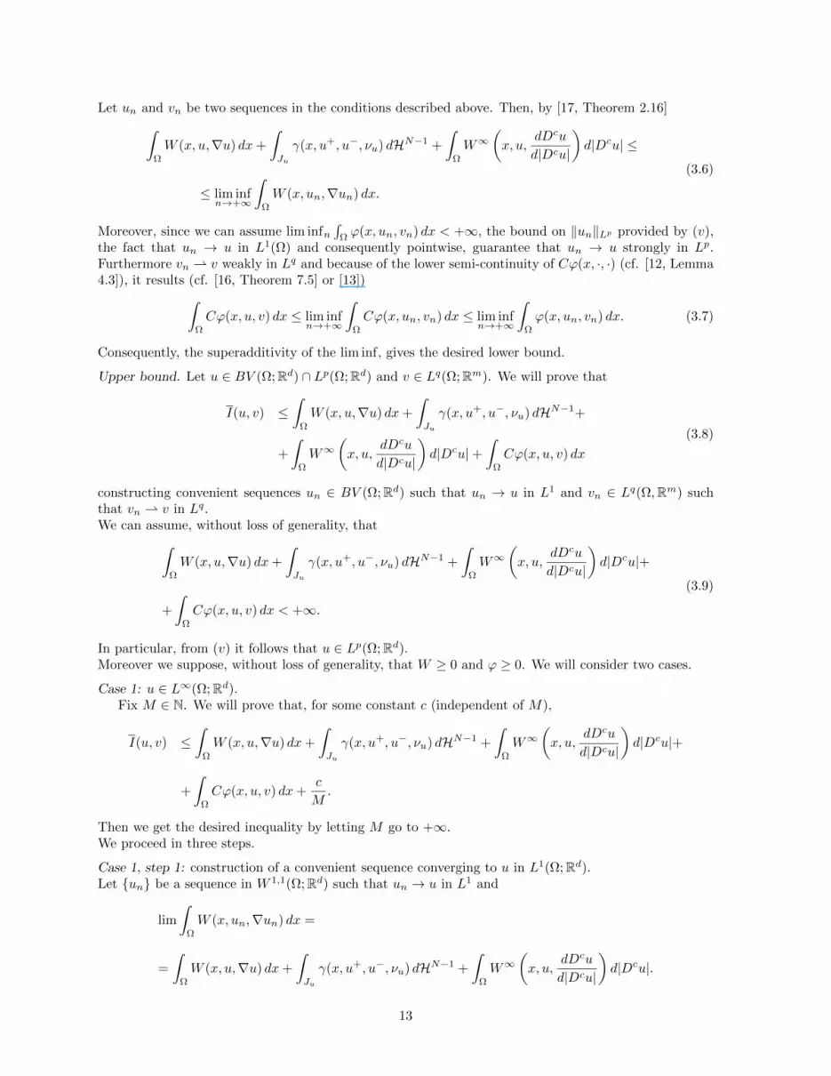
Let un and vn be two sequences in the conditions described above. Then, by [17, Theorem 2.16]∫Ω

W (x, u,∇u) dx+

∫Ju

γ(x, u+, u−, νu) dHN−1 +

∫Ω

W∞(x, u,

dDcu

d|Dcu|

)d|Dcu| ≤

≤ lim infn→+∞

∫Ω

W (x, un,∇un) dx.

(3.6)

Moreover, since we can assume lim infn∫

Ωϕ(x, un, vn) dx < +∞, the bound on ‖un‖Lp provided by (v),

the fact that un → u in L1(Ω) and consequently pointwise, guarantee that un → u strongly in Lp.Furthermore vn v weakly in Lq and because of the lower semi-continuity of Cϕ(x, ·, ·) (cf. [12, Lemma4.3]), it results (cf. [16, Theorem 7.5] or [13])∫

Ω

Cϕ(x, u, v) dx ≤ lim infn→+∞

∫Ω

Cϕ(x, un, vn) dx ≤ lim infn→+∞

∫Ω

ϕ(x, un, vn) dx. (3.7)

Consequently, the superadditivity of the lim inf, gives the desired lower bound.

Upper bound. Let u ∈ BV (Ω;Rd) ∩ Lp(Ω;Rd) and v ∈ Lq(Ω;Rm). We will prove that

I(u, v) ≤∫

Ω

W (x, u,∇u) dx+

∫Ju

γ(x, u+, u−, νu) dHN−1+

+

∫Ω

W∞(x, u,

dDcu

d|Dcu|

)d|Dcu|+

∫Ω

Cϕ(x, u, v) dx

(3.8)

constructing convenient sequences un ∈ BV (Ω;Rd) such that un → u in L1 and vn ∈ Lq(Ω,Rm) suchthat vn v in Lq.We can assume, without loss of generality, that∫

Ω

W (x, u,∇u) dx+

∫Ju

γ(x, u+, u−, νu) dHN−1 +

∫Ω

W∞(x, u,

dDcu

d|Dcu|

)d|Dcu|+

+

∫Ω

Cϕ(x, u, v) dx < +∞.

(3.9)

In particular, from (v) it follows that u ∈ Lp(Ω;Rd).Moreover we suppose, without loss of generality, that W ≥ 0 and ϕ ≥ 0. We will consider two cases.

Case 1: u ∈ L∞(Ω;Rd).Fix M ∈ N. We will prove that, for some constant c (independent of M),

I(u, v) ≤∫

Ω

W (x, u,∇u) dx+

∫Ju

γ(x, u+, u−, νu) dHN−1 +

∫Ω

W∞(x, u,

dDcu

d|Dcu|

)d|Dcu|+

+

∫Ω

Cϕ(x, u, v) dx+c

M.

Then we get the desired inequality by letting M go to +∞.We proceed in three steps.

Case 1, step 1: construction of a convenient sequence converging to u in L1(Ω;Rd).Let un be a sequence in W 1,1(Ω;Rd) such that un → u in L1 and

lim

∫Ω

W (x, un,∇un) dx =

=

∫Ω

W (x, u,∇u) dx+

∫Ju

γ(x, u+, u−, νu) dHN−1 +

∫Ω

W∞(x, u,

dDcu

d|Dcu|

)d|Dcu|.

13

This exists by [17, Theorem 2.16]. Next we will truncate the sequence un.Fix k such that ek − 1 > 2||u||L∞ . Then, hypothesis (3.9) together with the coercivity condition of Won ξ, cf. (i), and the fact that ϕ ≥ 0, imply that sup ||∇un||L1 is bounded by a constant independent ofthe sequence un. Thus

M−1∑i=0

∫x∈Ω: k+i≤ln(1+|un|)<k+i+1

(1 + |∇un|) dx =

∫x∈Ω: k≤ln(1+|un|)<k+M

(1 + |∇un|) dx

≤ |Ω|+ supn||∇un||L1

and so, for each n ∈ N, we can find i = i(n) ∈ 0, ...,M − 1 such that∫x∈Ω: k+i≤ln(1+|un|)<k+i+1

(1 + |∇un(x)|) dx ≤ |Ω|+ supn ||∇un||L1

M. (3.10)

For each n, and accordingly to the previous choice of i(n), consider τn : R+0 −→ [0, 1] such that τn ∈

C1(R+0 ), |τ ′n| ≤ 1,

τn(t) = 1, if 0 ≤ t < k + i(n) and τn(t) = 0, if t ≥ k + i(n) + 1.

We can now define the truncated sequence. Let gn(z) := τn(ln(1 + |z|)) z, and un(x) = gn(un). Since ina neighborhood of 0 the function τn(ln(1 + | · |)) is identically 1, gn is a Lipschitz, C1 function with

∇gn(z) =

τn(ln(1 + |z|)) I + τ ′n(ln(1 + |z|)) 1

1+|z|z⊗z|z| , if z 6= 0

I, if z = 0

and |∇gn(z)| ≤ c. So, by Theorem 3.96 in [2], un ∈ W 1,1(Ω;Rd), ∇un = ∇gn(un)∇unLN and |∇un| ≤c|∇un| which is bounded in L1 as observed above. Moreover ||un||L∞ ≤ ek+i(n)+1 − 1 ≤ ek+M − 1 andun → u in L1. Indeed, if u ≡ 0 then ||un||L1 ≤ ||un||L1 → 0. If not

||un − u||L1(Ω) =

∫x∈Ω: 0≤ln(1+|un|)<k+i(n)

|un(x)− u(x)| dx+

+

∫x∈Ω: k+i(n)≤ln(1+|un|)<k+i(n)+1

|un(x)− u(x)| dx+

+

∫x∈Ω: ln(1+|un|)≥k+i(n)+1

|u(x)| dx

≤ ||un − u||L1(Ω) +

∫x∈Ω: k+i(n)≤ln(1+|un|)<k+i(n)+1

|un(x)− un(x)| dx+

+||un − u||L1(Ω) + ||u||L∞(Ω) |x ∈ Ω : ln(1 + |un|) ≥ k + i(n) + 1|

≤ 2||un − u||L1(Ω) +

∫x∈Ω: k+i(n)≤ln(1+|un|)<k+i(n)+1

|un(x)| dx+

+||u||L∞(Ω) |x ∈ Ω : ln(1 + |un|) ≥ k + i(n) + 1|

these last terms converging to zero because un → u in L1 and because of the following estimates:

∫x∈Ω: k+i(n)≤ln(1+|un|)<k+i(n)+1

|un(x)| dx ≤∫x∈Ω: k+i(n)≤ln(1+|un|)<k+i(n)+1

ek+M − 1 dx

≤ (ek+M − 1)∣∣x ∈ Ω : |un| ≥ ek+i(n) − 1

∣∣≤ (ek+M − 1)

∣∣x ∈ Ω : |un − u| ≥ ||u||L∞(Ω)∣∣

≤ (ek+M − 1)||un − u||L1(Ω)

||u||L∞(Ω),

14

|x ∈ Ω : ln (1 + |un|) ≥ k + i(n) + 1| =∣∣∣x ∈ Ω : |un| ≥ ek+i(n)+1 − 1

∣∣∣≤

∣∣x ∈ Ω : |un − u| ≥ ||u||L∞(Ω)∣∣

≤||un − u||L1(Ω)

||u||L∞(Ω).

So, we have, in particular, that un converges to u in L1 and un clearly belongs to Lp(Ω;Rd).Case 1, step 2: construction of a convenient sequence vn weakly converging to v in Lq.

We have, by (v), [16, Theorem 6.68 and Remark 6.69 (ii)], for any w ∈ L1(Ω;Rd)∫Ω

Cϕ(x,w, v) dx = inf

lim infn→+∞

∫Ω

ϕ(x,w, vn) dx : vn ⊂ Lq(Ω;Rm), vn v in Lq

whenever the second term is finite.Since q > 1 and thus Lq

′(Ω;Rm) is separable, we can consider a sequence ψl of functions, dense in

Lq′(Ω;Rm).

Then, for each n ∈ N let vnj ∈ Lq(Ω;Rm) be such that∫Ω

Cϕ(x, un, v) dx = limj→+∞

∫Ω

ϕ(x, un, vnj ) dx

and

limj→+∞

∫Ω

(vnj − v)ψl dx = 0, ∀ l ∈ N.

We then extract a diagonalizing sequence vn in the following way: for each n ∈ N consider j(n) increasingand verifying ∣∣∣∣∫

Ω

(ϕ(x, un, v

nj(n))− Cϕ(x, un, v)

)dx

∣∣∣∣ ≤ 1

n∣∣∣∣∫Ω

(vnj(n) − v)ψl dx

∣∣∣∣ ≤ 1

n, l = 1, ..., n.

Define then vn = vnj(n). We have vn bounded in the Lq norm:∫Ω

|vn|q dx ≤ C∫

Ω

ϕ(x, un, vn) dx ≤ C

n+ C

∫Ω

Cϕ(x, un, v) dx ≤ C + C

∫Ω

ϕ(x, un, v) dx

this last term being bounded because un is a bounded sequence in L∞ and because of the growth condition(v) on ϕ.Moreover the density of ψl in Lq

′ensures that vn v in Lq. Indeed, let ψ ∈ Lq(Ω;Rm) and let δ > 0.

Consider l ∈ N such that ||ψl − ψ||Lq′ ≤ δ. Then, for sufficiently large n,∣∣∣∣∫Ω

(vn − v)ψ dx

∣∣∣∣ ≤ ∣∣∣∣∫Ω

(vn − v)(ψ − ψl) dx∣∣∣∣+

∣∣∣∣∫Ω

(vn − v)ψl dx

∣∣∣∣ ≤ ||vn − v||Lq ||ψl − ψ||Lq′ + δ ≤ cδ + δ.

Case 1, step 3: upper bound for I.Start remarking that

lim supn→+∞

∫Ω

ϕ(x, un, vn) dx ≤∫

Ω

Cϕ(x, u, v) dx.

Indeed,

lim supn→+∞

∫Ω

ϕ(x, un, vn) dx = lim supn→+∞

∫Ω

(ϕ(x, un, vn)− Cϕ(x, un, v) + Cϕ(x, un, v)) dx

≤ lim supn→+∞

(1

n+

∫Ω

Cϕ(x, un, v) dx

).

15

As observed in Remark 2.3, Cϕ(x, ·, v) is upper semi-continuous. By the pointwise convergence of untowards u (up to a subsequence), we have

lim supn→+∞

Cϕ(x, un, v) ≤ Cϕ(x, u, v).

Moreover the fact that un is bounded in L∞ and the hypothesis (v) allows to apply the “inverted” Fatou’slemma and get the desired inequality.Now we have∫

Ω

W (x, un,∇un) dx =

∫x∈Ω: 0≤ln(1+|un|)<k+i(n)

W (x, un,∇un) dx+

+

∫x∈Ω: k+i(n)≤ln(1+|un|)<k+i(n)+1

W (x, un,∇un) dx+

+

∫x∈Ω: ln(1+|un|)≥k+i(n)+1

W (x, 0, 0) dx

≤∫

Ω

W (x, un,∇un) dx+

∫x∈Ω: k+i(n)≤ln(1+|un|)<k+i(n)+1

C(1 + |∇un|) dx+

+C |x ∈ Ω : ln(1 + |un|) ≥ k + i(n) + 1|

(where it has been used the growth condition (i). Using the expression of un, by [2, Theorem 3.96], wehave |∇un| ≤ c|∇un| and so, using (3.10), we get

lim supn→+∞

∫x∈Ω: k+i(n)≤ln(1+|un|)<k+i(n)+1

C(1 + |∇un|) dx ≤ c|Ω|+ sup ||∇un||L1

M=

c

M

(note that c is independent of n and of the sequence un, and it doesn’t represent always the sameconstant).Moreover, since |x ∈ Ω : ln(1 + |un|) ≥ k + i(n) + 1| → 0 as n → +∞ (as already seen in the casewhere ||u||L∞ 6= 0) we get,

lim supn→+∞

∫Ω

W (x, un,∇un) dx ≤ limn→+∞

∫Ω

W (x, un,∇un) dx+c

M.

Note that if u = 0 we can still get |x ∈ Ω : ln(1 + |un|) ≥ k + i(n) + 1| → 0:

|x ∈ Ω : ln(1 + |un|) ≥ k + i(n) + 1| ≤∣∣x ∈ Ω : |un| ≥ ek+1 − 1

∣∣ ≤ ||un||L1

ek+1 − 1→ 0

since un → 0 in L1.Finally, we get, as desired,

I(u, v) ≤ lim infn→+∞

∫Ω

W (x, un,∇un) dx+

∫Ω

ϕ(x, un, vn) dx

≤ lim supn→+∞

∫Ω

W (x, un,∇un) dx+ lim supn→+∞

∫Ω

ϕ(x, un, vn) dx

≤∫

Ω

W (x, u,∇u) dx+

∫Ju

γ(x, u+, u−, νu) dHN−1 +

∫Ω

W∞(x, u,

dDcu

d|Dcu|

)d|Dcu|+

+c

M+

∫Ω

Cϕ(x, u, v) dx.

Case 2: arbitrary u ∈ BV (Ω;Rd) ∩ Lp(Ω;Rd).

16

To achieve the upper bound on this case, we will reduce ourselves to Case 1 by means of a truncatureargument developed in [17, Theorem 2.16, Step 4], in turn inspired by [3, Theorem 4.9]. We reproducethe same argument as in [17] for the reader’s convenience.Let φn ∈ C1

0 (Rd;Rd) be such that

φn(y) = y if y ∈ Bn(0), ‖∇φn‖L∞ ≤ 1,

and fix u ∈ BV (Ω;Rd) ∩ Lp(Ω;Rd).As proven in [3, Theorem 4.9], directly from the definitions and properties for the approximate dis-

continuity set and the triplets (u+, u−, νu) (see Subection 2.2), it results that

Jφn(u) ⊂ Ju,

(φn(u)+, φn(u)−, νφn(u)) = (φn(u+), φn(u−), νu) in Jφn(u).

Moreover one has|Dφn(u)|(B) ≤ |D(u)|(B), for every Borel set B ⊂ Ω. (3.11)

Consequentlyφn(u) ∈ BV (Ω;Rd) ∩ L∞(Ω;Rd).

Since φn(u)→ u in L1, by the lower semicontinuity of I (since q > 1) and by Case 1 we get

I(u, v) ≤ lim infn→+∞

[∫Ω

W (x, φn(u),∇φn(u)) dx+

∫Jφn(u)

γ(x, φn(u)+, φn(u)−, νφn(u)) dHN−1+

+

∫Ω

W∞(x, φn(u),

dDc(φn(u))

d|Dc(φn(u))|

)d|Dcφn(u)|+

∫Ω

Cϕ(x, φn(u), v) dx

].

By the upper semicontinuity of γ in all of its arguments as stated in [17, (c) of Lemma 2.15] and by thefact that γ(x, a, b, ν) ≤ C|a − b| for every (x, a, b, ν) ∈ Ω × Rd × Rd × SN−1 (see [17, (d) Lemma 2.15])and the properties of φn we have

γ(x, φn(u+), φn(u−), νu) ≤ C|u+ − u−|,

and so, by Fatou’s Lemma we obtain

lim supn→+∞

∫Jφn(u)

γ(x, φn(u)+, φn(u)−, νu) dHN−1 ≤∫Ju

γ(x, u+, u−, νu) dHN−1.

Moreover we have

lim supn→+∞

∫Ω

Cϕ(x, φn(u), v) dx =

∫Ω

Cϕ(x, u, v) dx (3.12)

Indeed, as already observed in step 2, Cϕ(x, ·, v) is upper semicontinuous and φn(u) is pointwise con-verging to u and thus we can apply the inverted Fatou’s lemma.For what concerns the other terms, setting Ωn := x ∈ Ω \ Ju : |u(x)| ≤ n, we have

lim supn→+∞

∫Ω

W (x, φn(u),∇φn(u)) dx =

= lim supn→+∞

[∫Ωn

W (x, φn(u),∇φn(u)) dx+

∫(Ω\Ωn)\Ju

W (x, φn(u),∇φn(u)) dx

]

≤∫

Ω

W (x, u,∇u) dx+ lim supn→+∞

C [|Ω \ Ωn|+ |Dφn(u)|((Ω \ Ωn) \ Ju)] .

17

On the other hand by (3.11) we deduce that

lim supn→+∞

|Dφn(u)|((Ω \ Ωn) \ Ju) ≤ lim supn→+∞

|Du|(Ω \ (Ωn ∪ Ju)) = 0

and so

lim supn→+∞

∫Ω

W (x, φn(u),∇φn(u)) dx ≤∫

Ω

W (x, u,∇u) dx.

Similarly

lim supn→+∞

∫Ω

W∞(x, φn(u),

dDcφn(u)

d|Dcφn(u)|

)d|Dcφn(u)| =

= lim supn→+∞

∫Ωn

W∞(x, φn(u),

dDcφn(u)

d|Dcφn(u)|

)d|Dcφn(u)|+

+ lim supn→+∞

∫(Ω\Ωn)\Ju

W∞(x, φn(u),

dDcφn(u)

d|Dcφn(u)|

)d|Dcφn(u)| ≤

≤∫

Ω

W∞(x, u,

dDcu

d|Dcu|

)d|Dcu|+ C lim sup

n→+∞[|Dφn(u)|((Ω \ Ωn) \ Ju)] =

=

∫Ω

W∞(x, u,

dDcu

d|Dcu|

)d|Dcu|.

This finishes the proof.

Part 2: q = 1.Lower bound. Let u ∈ BV (Ω;Rd) ∩ Lp(Ω;Rd), v ∈ L1(Ω;Rm), un ∈ BV (Ω;Rd) and vn ∈ L1(Ω;Rm)

such un → u strongly in L1 and vn v in L1. Then by Lemma 3.1 exactly as in the case q > 1, (3.6)continues to hold. Moreover [8, Theorem 1.1], ensures that∫

Ω

Cϕ(x, u, v) dx ≤ lim infn→+∞

∫Ω

ϕ(x, un, vn) dx.

Again the lower bound follows from the superadditivity of the liminf.Upper bound. Let u ∈ BV (Ω;Rd)∩Lp(Ω;Rd) and v ∈ L1(Ω;Rm). We aim to prove (3.8), constructing

convenient sequences un ∈ BV (Ω;Rd) and vn ∈ L1(Ω;Rm) with un → u in L1 and vn v in L1.Case 1. As in the case q > 1 we first assume that u ∈ L∞(Ω;Rd) and develop our proof in three steps.Case 1, step 1. The step 1 is identical to Case 1, step 1 proven for q > 1.Case 1, step 2. For what concerns this step, we preliminarly consider a continuous increasing functionθ : [0,+∞)→ [0,+∞) such that

limt→+∞

θ(t)

t= +∞. (3.13)

Then consider a decreasing sequence ε → 0 and take the functional Iε : BV (Ω;Rd) × L1(Ω;Rm) →R ∪ +∞, defined as

Iε(u, v) := I(u, v) + ε

∫Ω

θ(|v|) dx. (3.14)

Let C(ϕ(x, u, ·) + εθ(| · |)) be the convexification of ϕ(x, u, ·) + εθ(| · |) as in (1.6).By [16, Theorem 6.68 and Remark 6.69], we have that for every w ∈ L1(Ω;Rm)∫

Ω

C(ϕ(x,w, v) + εθ(|v|)) dx = inf

lim infn→+∞

∫Ω

(ϕ(x,w, vn) + εθ(|vn|)) dx : vn v in L1

whenever the second term is finite. Moreover the left hand side coincides with the sequentially weakly-L1

lower semicontinuous envelope. Consequently for every n ∈ N, let un be the sequence constructed in Case1, step 1 and let vnj ∈ L1(Ω;Rm) be such that vnj v in L1 as j → +∞ and∫

Ω

C(ϕ(x, un, v) + εθ(|v|)) dx = limj→+∞

∫Ω

(ϕ(x, un, vnj ) + εθ(|vnj |)) dx.

18

The proof now develops as in [16, Proposition 3.18]. The growth condition (v) and the fact that un isbounded in L∞ and thus in L1, entails that there exists a constant M such that

supn,j∈N

∫Ω

θ(|vnj |) dx ≤M. (3.15)

We observe that the growth conditions on θ guarantee that supn,j∈N ‖vnj ‖L1(Ω) ≤ C(M). Moreover theseparability of C0(Ω) allows us to consider a dense sequence of functions ψl.

Next, mimicking the argument used in the analogous step for q > 1, for every ε > 0 we construct adiagonalizing sequence vn as follows. For each n ∈ N consider j(n) increasing and such that∣∣∣∣∫

Ω

(ϕ(x, un, v

nj(n)) + εθ(|vnj(n)|)− C(ϕ(x, un, v) + εθ(|v|))

)dx

∣∣∣∣ ≤ 1

n∣∣∣∣∫Ω

(vnj(n) − v)ψl dx

∣∣∣∣ ≤ 1

n, l = 1, . . . , n.

Define vn := vnj(n). The bounds on θ, the fact that un is bounded in L1 and the separability of C0(Ω) guar-

antee that vn? v in M(Ω) and moreover, (3.15), Dunford-Pettis’ theorem entail that the convergence

of vn towards v is weak-L1.Case 1, step 3. Arguing as in the first part of Case 1, step 3 for q > 1, we can prove that

lim supn→+∞

∫Ω

(ϕ(x, un, vn) + εθ(|vn|)) dx ≤∫

Ω

C(ϕ(x, u, v) + εθ(|v|)) dx.

Next we define

Iε(u, v) := inflim infn→+∞

Iε(un, vn) : (un, vn) ∈ BV (Ω;Rd)× L1(Ω;Rm), un → u in L1, vn v in L1.(3.16)

The same argument of the last part in Case 1, step 3, for q > 1, allows to prove that

Iε(u, v) ≤∫

Ω

W (x, u,∇u) dx+

∫Ju

γ(x, u+, u−, νu) dHN−1+

+

∫Ω

W∞(x, u,

dDcu

d|Dcu|

)d|Dcu|+

∫Ω

C (ϕ(x, u, v) + εθ(|v|)) dx(3.17)

for every u ∈ BV (Ω;Rd) ∩ L∞(Ω;Rd) and v ∈ L1(Ω;Rm). On the other hand we observe that thesequence Iε(u, v) is increasing in ε and I ≤ Iε for every ε. Moreover by virtue of the increasing behaviourin ε of ϕ+ εθ, invoking [16, Proposition 4.100] it results that for every (x, u) ∈ Ω× Rd, we have

infεC (ϕ(x, u, v) + εθ(|v|)) = lim

ε→0C (ϕ(x, u, v) + εθ(|v|)) = Cϕ(x, u, v).

Thus applying Lebesgue monotone convergence theorem we have

I(u, v) ≤ limε→0

Iε(u, v) = limε→0

(∫Ω

W (x, u,∇u) dx+

∫Ju

γ(x, u+, u−, νu) dHN−1+

+

∫Ω

W∞(x, u,

dDcu

d|Dcu|

)d|Dcu|+

∫Ω

C (ϕ(x, u, v) + εθ(|v|)) dx)

=

=

∫Ω

W (x, u,∇u) dx+

∫Ju

γ(x, u+, u−, νu)dHN−1 +

∫Ω

W∞(x, u,

dDcu

d|Dcu|

)d|Dcu|+

∫Ω

Cϕ(x, u, v) dx,

(3.18)for every (u, v) ∈ (BV (Ω;Rd) ∩ L∞(Ω;Rd))× L1(Ω;Rm).

Case 2. Now we consider u ∈ BV (Ω;Rd) ∩ Lp(Ω;Rd) and v ∈ L1(Ω;Rm).

19

To achieve the upper bound we can preliminarly observe that, a proof entirely similar to [16, Proposi-tion 3.18], guarantees that for every ε > 0, the functional Iε(u, v), defined in (3.16) is sequentially weaklylower semicontinuous with respect to the topology L1(Ω;Rd)strong×L1(Ω;Rm)weak. Thus, arguing exactlyas in the Case 2, for q > 1, we have that

Iε(u, v) ≤∫

Ω

W (x, u,∇u) dx+

∫Ju

γ(x, u+, u−, νu) dHN−1 +

∫Ω

W∞(x, u,

dDcu

d|Dcu|

)d|Dcu|+

+

∫Ω

C(ϕ(x, u, v) + εθ(|v|)) dx.

(3.19)Finally the monotonicity argument for ε invoked in the Case 1, step 3 for q = 1 can be recalled also in

this context leading to the same inequality in (3.18) for every u ∈ BV (Ω;Rd) ∩ Lp(Ω;Rd) and for everyv ∈ L1(Ω;Rm), and that concludes the proof of (3.8).

Now we present the proof of Theorem 1.3, which is much easier than the latter one, since, by virtue of

the continuous embedding of BV (Ω;Rd) in LNN−1 (Ω;Rd), it does not involve any truncature argument.

Proof of Theorem 1.3. We omit the details of the proof since it develops in the same way as that ofTheorem 1.1. First we invoke Corollary 3.2 and assume without loss of generality that W is quasiconvexin the last variable. Then we prove a lower bound for the relaxed energy and finally we show that thelower bound is also an upper bound. As in Theorem 1.1 we may consider two separate cases: q > 1 and

q = 1.Lower bound for the cases q = 1 and q > 1. The proof of the lower bound is identical to that of Theorem1.1.

Upper bound, case q > 1. Let u ∈ BV (Ω;Rd) and v ∈ Lq(Ω;Rm). We can assume∫Ω

W (x, u,∇u) dx+

∫Ju

γ(x, u+, u−, νu) dHN−1 +

∫Ω

W∞(x, u,

dDcu

d|Dcu|

)d|Dcu|+

+

∫Ω

Cϕ(x, u, v) dx < +∞.(3.20)

Without loss of generality, we assume also that W and ϕ ≥ 0. Applying Lemma [17, Theorem 2.16],we can get a sequence un in W 1,1(Ω;Rd) such that un → u in L1 and

lim

∫Ω

W (x, un,∇un) dx =

∫Ω

W (x, u,∇u) dx+

∫Ju

γ(x, u+, u−, νu) dHN−1+

+

∫Ω

W∞(x, u,

dDcu

d|Dcu|

)d|Dcu|.

We observe that, by the coercivity condition on W and by (3.20), ∇un is bounded in L1. Moreover,

the continuous embedding of BV (Ω;Rd) in LNN−1 (Ω;Rd), imply that un is bounded in L

NN−1 (Ω;Rd) and

thus in Lp(Ω;Rd) since we are assuming 1 ≤ p ≤ NN−1 .

Then, as in the proof of Theorem 1.1, Case 1, step 2, q > 1 we can construct a recovery sequence vnusing the relaxation theorem [16, Theorem 6.68] and the same diagonalizing argument. We emphasizethat there is no need to make a preliminary truncature of the recovery sequence un. Indeed, to ensurethat vn is bounded in Lq(Ω;Rm) (required to obtain the weak convergence of vn towards v in Lq) itsuffices to use the growth condition of ϕ and the fact that un is bounded in Lp.

Therefore it is possible to get vn v in Lq and such that

lim supn→+∞

∫Ω

ϕ(x, un, vn) dx ≤∫

Ω

Cϕ(x, u, v) dx.

The upper bound then follows by the sub-additivity of the limsup.

20

Upper bound, case q = 1. In analogy with the case q > 1 there is no need of truncature because of the

continuous embedding of BV in LNN−1 . As for Theorem 1.1 it suffices to approximate the functional I by Iε

in (3.14) and consequently it is enough to use, for the correspective relaxed functional, the diagonalizationargument adopted in Theorem 1.1, Case 1, step 2 for q = 1 via an application of Dunford-Pettis’ theorem.Finally the monotonicity behaviour in ε of Iε, the approximation of the energy densities allowed by [16,Proposition 4.100] and the Lebegue monotone convergence theorem conclude the proof.

Acknowledgements The authors would like to thank Irene Fonseca and Giovanni Leoni for theirinvaluable comments on the subject of this paper and acknowledge the Center for Nonlinear Analysis,Carnegie Mellon University, Pittsburgh (PA) for the kind hospitality and support.

A.M. Ribeiro thanks Universita di Salerno and E. Zappale thanks Universidade Nova de Lisboa fortheir support and hospitality.

The research of A. M. Ribeiro was partially supported by Fundacao para a Ciencia e Tecnolo-gia, through the Pos-Doc Grant SFRH/BPD/34477/2006, Financiamento Base 2010-ISFL/1/297 fromFCT/MCTES/PT, PTDC/MAT/109973/2009 and UTA-CMU/MAT/0005/2009.

References

[1] L. Ambrosio & G. Dal Maso, On the Relaxation in BV (Ω;Rm) of Quasi-convex Integrals, Journalof Functional Analysis, 109, (1992), 76-97.

[2] L. Ambrosio, N. Fusco & D. Pallara, Functions of Bounded Variation and Free DiscontinuityProblems, Clarendon Press, Oxford, (2000).

[3] L. Ambrosio, S. Mortola & V. M. Tortorelli, Functionals with linear growth defined on vectorvalued BV functions, J. Math. Pures Appl., IX. Ser. 70, No. 3, (1991), 269-323.

[4] J.-F. Aujol, G. Aubert, L. Blanc-Feraud & A. Chambolle, Image decomposition into abounded variation component and an oscillating component, Journal of Mathematical Imaging andVision, 22 (1), (2005), 71-88.

[5] J.-F. Aujol, G. Aubert, L. Blanc-Feraud & A. Chambolle, Decomposing an image: Appli-cation to SAR images, Scale-Space ’03, Vol. 2695 of Lecture Notes in Computer Science, (2003),297-312.

[6] J.-F. Aujol & S.H. Kang, Color image decomposition and restoration, Journal of Visual Commu-nication and Image Representation, 17, No. 4, (2006), 916-928.

[7] J. F. Babadjian, E. Zappale & H. Zorgati, Dimensional reduction for energies with linear growthinvolving the bending moment, J. Math. Pures Appl. (9), 90, No. 6, (2008), 520-549.

[8] A. Braides, I. Fonseca & G. Leoni, A-quasiconvexity: relaxation and homogenization, ESAIM:Control, Optimization and Calculus of Variations, 5, (2000), 539-577.

[9] G. Carita, A.M. Ribeiro & E. Zappale, An homogenization result in W 1,p × Lq, to appear inJournal of Convex Analysis, 18, No.4, (2011).

[10] G. Carita, A.M. Ribeiro & E. Zappale, Relaxation for some integral functionals in W 1,pw ×Lqw,

to appear in Actas ENSPM.

[11] B. Dacorogna, Direct Methods in the Calculus of Variations, Second Edition, Applied Mathemat-ical Sciences, 78, Berlin: Springer, xii, (2008), 619 p.

[12] G. Dal Maso, I. Fonseca, G. Leoni & M. Morini, Higher order quasiconvexity reduces toquasiconvexity, Arch. Rational Mech. Anal, 171, No. 51, (2004), 55-81.

21

[13] I. Ekeland & R. Temam, Convex analysis and variational problems, Studies in Mathematicsand its Applications, Vol. 1. Amsterdam - Oxford: North-Holland Publishing Company; New York:American Elsevier Publishing Company, Inc. IX, 402 p., (1976).

[14] I. Fonseca, D. Kinderlehrer & P. Pedregal, Relaxation in BV ×L∞ of functionals dependingon strain and composition, Lions, Jacques-Louis (ed.) et al., Boundary value problems for partialdifferential equations and applications. Dedicated to Enrico Magenes on the occasion of his 70thbirthday. Paris: Masson. Res. Notes Appl. Math., 29, (1993), 113-152.

[15] I. Fonseca, D. Kinderlehrer & P. Pedregal, Energy functionals depending on elastic strainand chemical composition, Calc. Var. Partial Differential Equations, 2, (1994), 283-313.

[16] I. Fonseca & G. Leoni, Modern Methods in the Calculus of Variations: Lp Spaces, Springer(2007).

[17] I. Fonseca & S. Muller, Relaxation of quasiconvex functionals in BV (Ω;Rp) for integrandsf(x, u,∇u), Arch. Rational Mech. Anal., 123, (1993), 1-49.

[18] I. Fonseca & P. Rybka, Relaxation of multiple integrals in the space BV (Ω,Rp), Proc. R. Soc.Edinb., Sect. A 121, No. 3-4, (1992), 321-348.

[19] Y. Meyer, Oscillating pattern in image processing and nonlinear evolution equations. The fifteenthDean Jacqueline B. Lewis memorial lectures. University Lecture Series, 22, Providence, RI. AmericanMathematical Society (AMS). (2001)

[20] S. Osher, A. Sole & L. A. Vese, Image decomposition and restoration using total variationminimization and the H−1 norm, SIAM Multiscale Model. Simul., 1, No. 3, (2003), 349-370 .

[21] L. I. Rudin, S. Osher & E. Fatemi, Nonlinear total variation based noise removal algorithms,Physica D, 60, No. 14, (1992) 259-268.

[22] L. A. Vese & S. Osher, Modeling textures with total variation minimization and oscillating patternsin image processing, J. Sci. Comput., 19, No. 13, (2003), 553-572.

[23] L. A. Vese & S. Osher, Image denoising and decomposition with total variation minimization andoscillatory functions, Journal of Mathematical Imaging and Vision, 20, (2004), 7-18.

22