Embed Size (px)
Citation preview
remote sensing
Article
Hyperspectral Image Super-Resolution via AdaptiveDictionary Learning and Double `1 Constraint
Songze Tang 1,*, Yang Xu 2, Lili Huang 3,4 and Le Sun 5
1 Department of Criminal Science and Technology, Nanjing Forest Police College, Nanjing 210023, China2 School of Computer Science and Engineering, Nanjing University of Science and Technology,
Nanjing 210094, China; [email protected] School of Science, Guangxi University of Science and Technology, Liuzhou 545006, China;
[email protected] School of Computer Science and Technology, Jinling Institute of Technology, Nanjing 211169, China5 School of Computer and Software, Nanjing University of Information Science and Technology,
Nanjing 210044, China; [email protected]* Correspondence: [email protected]; Tel.: +86-137-7055-8030
Received: 24 October 2019; Accepted: 25 November 2019; Published: 27 November 2019 �����������������
Abstract: Hyperspectral image (HSI) super-resolution (SR) is an important technique for improvingthe spatial resolution of HSI. Recently, a method based on sparse representation improved theperformance of HSI SR significantly. However, the spectral dictionary was learned under a fixedsize, empirically, without considering the training data. Moreover, most of the existing methodsfail to explore the relationship among the sparse coefficients. To address these crucial issues,an effective method for HSI SR is proposed in this paper. First, a spectral dictionary is learned,which can adaptively estimate a suitable size according to the input HSI without any prior information.Then, the proposed method exploits the nonlocal correlation of the sparse coefficients. Double `1
regularized sparse representation is then introduced to achieve better reconstructions for HSI SR.Finally, a high spatial resolution HSI is generated by the obtained coefficients matrix and the learnedadaptive size spectral dictionary. To evaluate the performance of the proposed method, we conductexperiments on two famous datasets. The experimental results demonstrate that it can outperformsome relatively state-of-the-art methods in terms of the popular universal quality evaluation indexes.
Keywords: hyperspectral image super-resolution; sparse representation; adaptive dictionary learning;double `1
1. Introduction
Hyperspectral sensors can capture images with many contiguous and very narrow spectral bandsthat span the visible, near-infrared, and mid-infrared portions of the spectrum [1,2]. Thus, hyperspectralimage (HSI) can provide fine spectral feature differences, to distinguish various materials, which canbe widely and successfully used for many applications, such as object classification [3,4], tracking [5],recognition [6], and remote sensing [7,8]. Due to various hardware limitations, real captured HSIusually has low spatial resolution (LR), which significantly limits its application. However, it is noteffective to enhance spatial resolution by improving the imaging quality of the hyperspectral sensors,and a breakthrough in hardware will be difficult and costly. Alternatively, HSI super-resolution (SR)has been proposed to generate a high spatial resolution (HR) HSI by fusing a high spectral resolutionimage, such as HSI, with an image, such as panchromatic image [9–16] or a multispectral image(MSI) [17–30].
Remote Sens. 2019, 11, 2809; doi:10.3390/rs11232809 www.mdpi.com/journal/remotesensing
Remote Sens. 2019, 11, 2809 2 of 22
1.1. Related Work
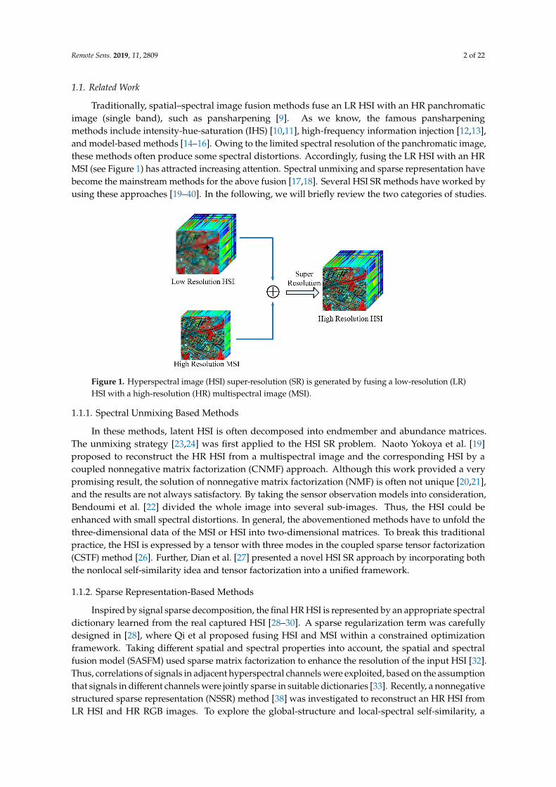
Traditionally, spatial–spectral image fusion methods fuse an LR HSI with an HR panchromaticimage (single band), such as pansharpening [9]. As we know, the famous pansharpeningmethods include intensity-hue-saturation (IHS) [10,11], high-frequency information injection [12,13],and model-based methods [14–16]. Owing to the limited spectral resolution of the panchromatic image,these methods often produce some spectral distortions. Accordingly, fusing the LR HSI with an HRMSI (see Figure 1) has attracted increasing attention. Spectral unmixing and sparse representation havebecome the mainstream methods for the above fusion [17,18]. Several HSI SR methods have worked byusing these approaches [19–40]. In the following, we will briefly review the two categories of studies.
Figure 1. Hyperspectral image (HSI) super-resolution (SR) is generated by fusing a low-resolution (LR)HSI with a high-resolution (HR) multispectral image (MSI).
1.1.1. Spectral Unmixing Based Methods
In these methods, latent HSI is often decomposed into endmember and abundance matrices.The unmixing strategy [23,24] was first applied to the HSI SR problem. Naoto Yokoya et al. [19]proposed to reconstruct the HR HSI from a multispectral image and the corresponding HSI by acoupled nonnegative matrix factorization (CNMF) approach. Although this work provided a verypromising result, the solution of nonnegative matrix factorization (NMF) is often not unique [20,21],and the results are not always satisfactory. By taking the sensor observation models into consideration,Bendoumi et al. [22] divided the whole image into several sub-images. Thus, the HSI could beenhanced with small spectral distortions. In general, the abovementioned methods have to unfold thethree-dimensional data of the MSI or HSI into two-dimensional matrices. To break this traditionalpractice, the HSI is expressed by a tensor with three modes in the coupled sparse tensor factorization(CSTF) method [26]. Further, Dian et al. [27] presented a novel HSI SR approach by incorporating boththe nonlocal self-similarity idea and tensor factorization into a unified framework.
1.1.2. Sparse Representation-Based Methods
Inspired by signal sparse decomposition, the final HR HSI is represented by an appropriate spectraldictionary learned from the real captured HSI [28–30]. A sparse regularization term was carefullydesigned in [28], where Qi et al proposed fusing HSI and MSI within a constrained optimizationframework. Taking different spatial and spectral properties into account, the spatial and spectralfusion model (SASFM) used sparse matrix factorization to enhance the resolution of the input HSI [32].Thus, correlations of signals in adjacent hyperspectral channels were exploited, based on the assumptionthat signals in different channels were jointly sparse in suitable dictionaries [33]. Recently, a nonnegativestructured sparse representation (NSSR) method [38] was investigated to reconstruct an HR HSI fromLR HSI and HR RGB images. To explore the global-structure and local-spectral self-similarity, a
Remote Sens. 2019, 11, 2809 3 of 22
self-similarity constrained sparse-representation (SSCSR) model was proposed by Han et. al [39].Owing to the complex structures in HSI, superpixel-based sparse-representation (SSR) model canextract the spectral features effectively [40].
1.2. Motivation and Contributions
Although the aforementioned methods gave us impressive recovery performance, we can produceeven better fused results from two aspects. On the one hand, the spectral basis (or the dictionary)generally has many atoms, whose sizes range from hundreds to hundreds of thousands, according tothe training data. Thus, learning an adaptive size dictionary can represent the data compactly andaccurately. On the other hand, due to the nonlocal correlations existing in natural images [41,42],the sparse coefficients are not randomly distributed. Therefore, it is possible to generate the highspatial resolution HSI faithfully by exploiting the nonlocal similarity of these coefficients.
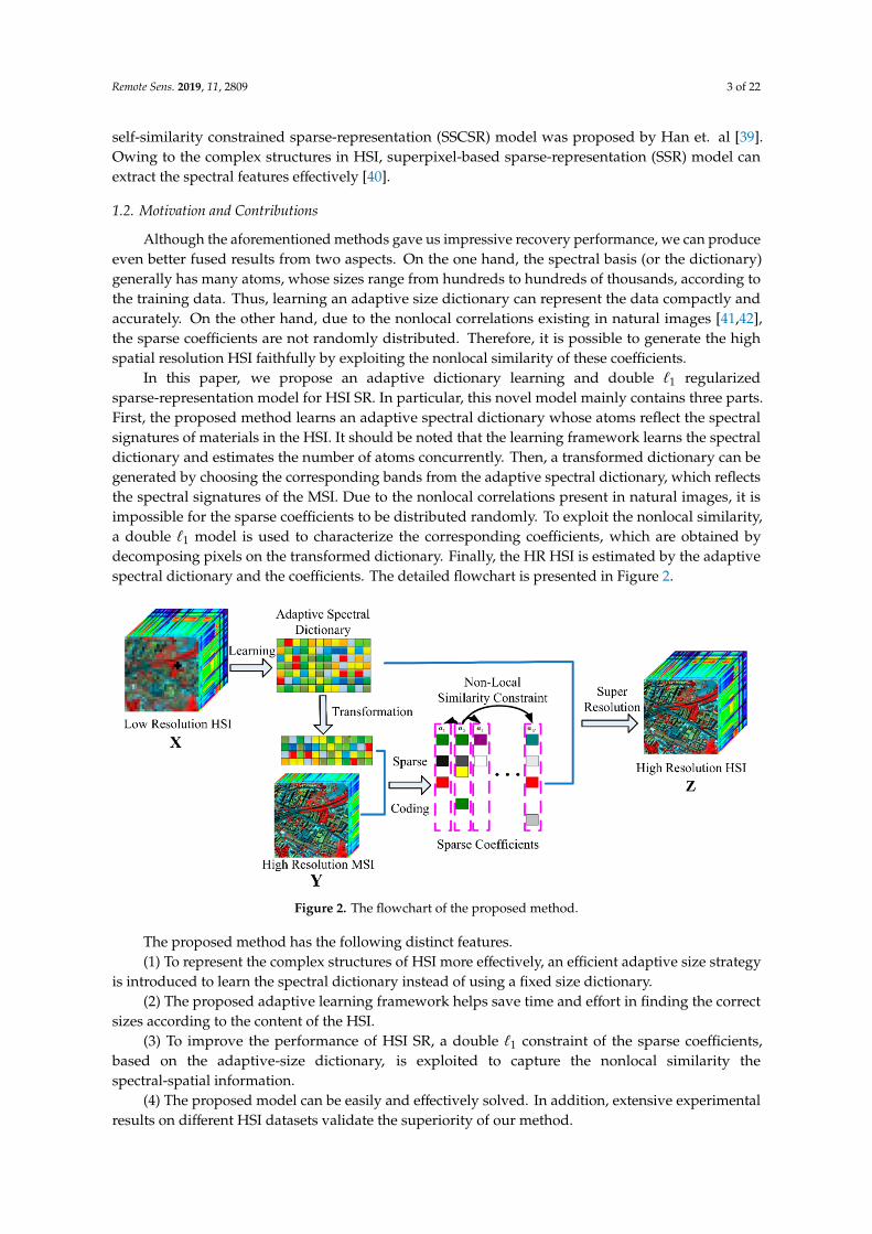
In this paper, we propose an adaptive dictionary learning and double `1 regularizedsparse-representation model for HSI SR. In particular, this novel model mainly contains three parts.First, the proposed method learns an adaptive spectral dictionary whose atoms reflect the spectralsignatures of materials in the HSI. It should be noted that the learning framework learns the spectraldictionary and estimates the number of atoms concurrently. Then, a transformed dictionary can begenerated by choosing the corresponding bands from the adaptive spectral dictionary, which reflectsthe spectral signatures of the MSI. Due to the nonlocal correlations present in natural images, it isimpossible for the sparse coefficients to be distributed randomly. To exploit the nonlocal similarity,a double `1 model is used to characterize the corresponding coefficients, which are obtained bydecomposing pixels on the transformed dictionary. Finally, the HR HSI is estimated by the adaptivespectral dictionary and the coefficients. The detailed flowchart is presented in Figure 2.
Figure 2. The flowchart of the proposed method.
The proposed method has the following distinct features.(1) To represent the complex structures of HSI more effectively, an efficient adaptive size strategy
is introduced to learn the spectral dictionary instead of using a fixed size dictionary.(2) The proposed adaptive learning framework helps save time and effort in finding the correct
sizes according to the content of the HSI.(3) To improve the performance of HSI SR, a double `1 constraint of the sparse coefficients,
based on the adaptive-size dictionary, is exploited to capture the nonlocal similarity thespectral-spatial information.
(4) The proposed model can be easily and effectively solved. In addition, extensive experimentalresults on different HSI datasets validate the superiority of our method.
Remote Sens. 2019, 11, 2809 4 of 22
2. Mothodology (or Materials and Methods)
2.1. The Traditional Sparse-Representation Method
Let X ∈ RB×n be the LR HSI, where n = a1 × a2. Terms a1 and a2 are the width and height of Xin spatial resolution, respectively. Term B indicates the spectral dimension. The acquired HR MSI isY ∈ Rb×N, where N = a3 × a4, a3 � a1, a4 � a2 and B� b. Therefore, HSI SR aims to estimate an HRHSI Z ∈ RB×N by using X and Y. In general, the relationship between X, Y, and the latent HSI Z can bemodelled as follows:
X = ZH (1)
Y = PZ (2)
where H ∈ RN×n denotes a degradation operator, and P ∈ Rb×B is a transform matrix.As a promising fusion technique, sparse representation has achieved great success [32,34,38,39].
In these methods, each pixel, zi ∈ RB, in Z ∈ RB×N is often represented via the following linearcombination:
zi = Dαi + ei (3)
where D ∈ RB×K represents a spectral dictionary, αi ∈ RK is the corresponding representation coefficientassumed to be sparse, and ei is the representation error.
According to Equation (1), each pixel, xi ∈ RB, can also be represented as follows:
xi =n∑
j=1Hi, jzi =
n∑j=1
Hi, j(Dαi) = Dn∑
j=1Hi, jαi
= Dβi + ti
(4)
where βi ∈ RK is the representation coefficient in the spectral dictionary, D, Hi, j denotes the elementof the i-th row and the j-th column, and ti is the residual. According to Equations (2) and (3), pixel,yi ∈ Rb, of the MSI, Y, can be mathematically formulated as follows:
yi = Pzi ≈ PDαi (5)
By combining Equations (4) and (5), it is easy to obtain the spectral dictionary, D, as well as thecorresponding coefficients matrix, A = [α1,α2, . . . ,αN] ∈ RK×N. Finally, we can generate the HR HSI,
Z, from the following equation:Z ≈ DA (6)
2.2. The Proposed Method
Due to the complex structures in HSI, it is not reasonable that different variations arerepresented by a dictionary with a fixed size in traditional methods. In other words,the traditional sparse-representation model cannot represent the complex structures of HSI accurately.Thus, we propose the learning of a spectral dictionary with an adaptive size, according to the contextin the captured area. Furthermore, double `1 prior of the sparse coefficients is exploited to improveHSI SR quality.
2.2.1. Adaptive Spectral Dictionary Learning
Traditionally, the spectral dictionary D ∈ RB×K was usually learned from a set of training exams{x1, . . . , xn}:
minD,B
1n
n∑i=1
{∥∥∥xi −Dβi∥∥∥2
2 + λ∥∥∥βi
∥∥∥1
}(7)
Remote Sens. 2019, 11, 2809 5 of 22
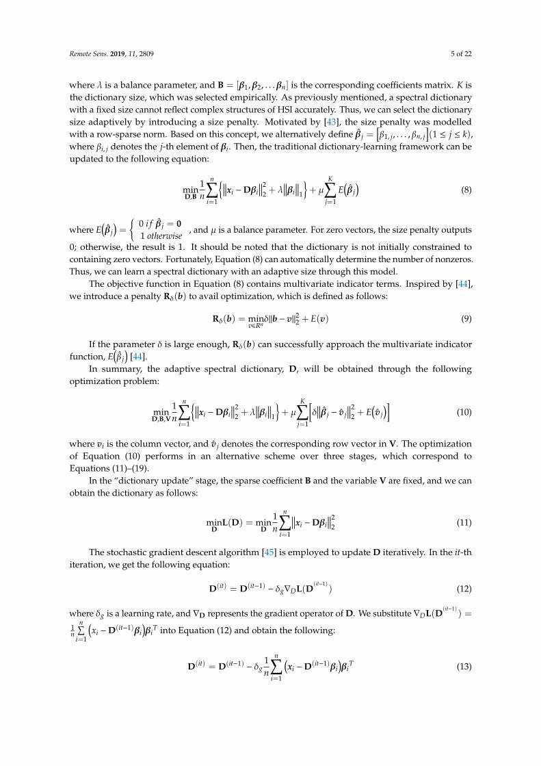
where λ is a balance parameter, and B = [β1,β2, . . .βn] is the corresponding coefficients matrix. K isthe dictionary size, which was selected empirically. As previously mentioned, a spectral dictionarywith a fixed size cannot reflect complex structures of HSI accurately. Thus, we can select the dictionarysize adaptively by introducing a size penalty. Motivated by [43], the size penalty was modelledwith a row-sparse norm. Based on this concept, we alternatively define β̂ j =
[β1, j, . . . , βn, j
](1 ≤ j ≤ k),
where βi, j denotes the j-th element of βi. Then, the traditional dictionary-learning framework can beupdated to the following equation:
minD,B
1n
n∑i=1
{∥∥∥xi −Dβi∥∥∥2
2 + λ∥∥∥βi
∥∥∥1
}+ µ
K∑j=1
E(β̂ j
)(8)
where E(β̂ j
)=
{0 i f β̂ j = 01 otherwise
, and µ is a balance parameter. For zero vectors, the size penalty outputs
0; otherwise, the result is 1. It should be noted that the dictionary is not initially constrained tocontaining zero vectors. Fortunately, Equation (8) can automatically determine the number of nonzeros.Thus, we can learn a spectral dictionary with an adaptive size through this model.
The objective function in Equation (8) contains multivariate indicator terms. Inspired by [44],we introduce a penalty Rδ(b) to avail optimization, which is defined as follows:
Rδ(b) = minv∈Rn
δ‖b− v‖22 + E(v) (9)
If the parameter δ is large enough, Rδ(b) can successfully approach the multivariate indicatorfunction, E
(β̂ j
)[44].
In summary, the adaptive spectral dictionary, D, will be obtained through the followingoptimization problem:
minD,B,V
1n
n∑i=1
{∥∥∥xi −Dβi∥∥∥2
2 + λ∥∥∥βi
∥∥∥1
}+ µ
K∑j=1
[δ∥∥∥β̂ j − v̂ j
∥∥∥22 + E
(v̂ j
)](10)
where vi is the column vector, and v̂ j denotes the corresponding row vector in V. The optimizationof Equation (10) performs in an alternative scheme over three stages, which correspond toEquations (11)–(19).
In the “dictionary update” stage, the sparse coefficient B and the variable V are fixed, and we canobtain the dictionary as follows:
minD
L(D) = minD
1n
n∑i=1
∥∥∥xi −Dβi∥∥∥2
2 (11)
The stochastic gradient descent algorithm [45] is employed to update D iteratively. In the it-thiteration, we get the following equation:
D(it) = D(it−1)− δg∇DL(D
(it−1)) (12)
where δg is a learning rate, and ∇D represents the gradient operator of D. We substitute ∇DL(D(it−1)
) =
1n
n∑i=1
(xi −D(it−1)βi
)βi
T into Equation (12) and obtain the following:
D(it) = D(it−1)− δg
1n
n∑i=1
(xi −D(it−1)βi
)βi
T (13)
Remote Sens. 2019, 11, 2809 6 of 22
Similar to the “dictionary update” stage, with the other variables fixed, we update the sparsecoefficient B according to the following equation:
minB
1n
n∑i=1
{∥∥∥xi −Dβi∥∥∥2
2 + λ∥∥∥βi
∥∥∥1
}+ µ
K∑j=1
δ∥∥∥β̂ j − v̂ j
∥∥∥22
= minB
1n
n∑i=1
{∥∥∥xi −Dβi∥∥∥2
2 + λ∥∥∥βi
∥∥∥1 + nµδ
∥∥∥βi − vi∥∥∥2
2
} (14)
For each i, Equation (14) is independent. Thus, finding the optimal{βi
}solves the following
independent problems of the form:
minβi
∥∥∥xi −Dβi∥∥∥2
2 + λ∥∥∥βi
∥∥∥1 + nµδ
∥∥∥βi − vi∥∥∥2
2 (15)
Let
1
Υ =
[xi√
nµδvi
], Θ =
[D√nµδI
], and Equation (15) can be written as follows:
minβi
∥∥∥
1
Υ −Θβi∥∥∥2
2 + λ∥∥∥βi
∥∥∥1 (16)
This is a combination of the quadratic and `1 sparse terms; thus, the iterative shrinkagethresholding algorithm [46] is popular for solving this efficiently. In the it-th iteration, we obtain thefollowing equation:
βi(it) =
υ(it−1)− 2λ · sgn
(υ(it−1)
)0
∣∣∣
1
Υ (it−1)∣∣∣ > 2λ∣∣∣
1
Υ (it−1)∣∣∣ ≤ 2λ
(17)
where υ(it−1) = 12βi
(it−1) +(Θ(it−1)
)T(
1
Υ (it−1)−Θ(it−1)βi
(it−1)).
Finally, we update the variable V fixed D and B:
minv̂ j∈V
K∑j=1
[δ∥∥∥β̂ j − v̂ j
∥∥∥22 + E
(v̂ j
)], (18)
which can be decomposed to K independent functions with respect to j:
minv̂ jδ∥∥∥β̂ j − v̂ j
∥∥∥22 + E
(v̂ j
)(19)
According to [44], we can obtain its solution as follows:
v̂ j =
δ∥∥∥β̂ j
∥∥∥22
1
∥∥∥β̂ j∥∥∥2
2 <1δ
otherwise(20)
Algorithm 1: Adaptive Spectral Dictionary Learning
Input: the training examples {x1, . . . , xn}, the regularization parameters λ= 0.2, µ= 0.001.Initialize δ= 1, it = 1, V0 = 0K×n,while δ < 106 doInput Vit−1, Dit−1, update Bit by (17);Input Bit, update Vit by (20);Input Bit and Dit−1, update Dit by (13);it← it + 1 ;δ← 2δend whileOutput: the spectral dictionary D = Dit
Remote Sens. 2019, 11, 2809 7 of 22
2.2.2. Double `1 Regularization
This subsection addresses the problem of how to obtain the sparse coefficient αi from the HR MSI,Y, and the spectral dictionary, D, associated with Equation (5). Traditionally, αi is obtained with a `1
constraint as follows:αi = argmin
αi
∥∥∥yi −Dαi∥∥∥2
2 + λ1‖αi‖1 (21)
where D = PD. In Equation (21), the sparse coefficient of each αi is computed independently.Actually, each pixel has a strong correlation with its nonlocal similar neighbors in the HR HSI. Thus, it isimpossible for the sparse coefficients to be distributed randomly. In other words, even better SR resultswill be produced if the nonlocal similarities of the sparse coefficients are considered.
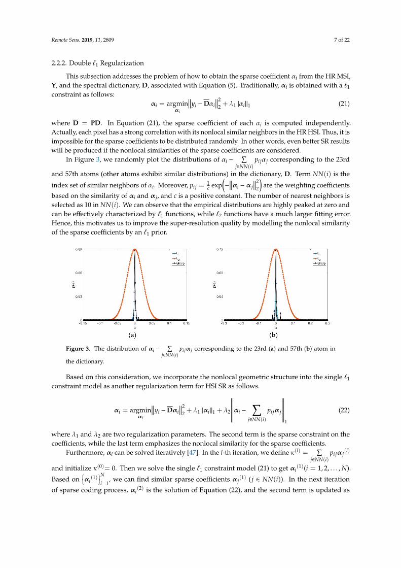
In Figure 3, we randomly plot the distributions of αi −∑
j∈NN(i)pi jα j corresponding to the 23rd
and 57th atoms (other atoms exhibit similar distributions) in the dictionary, D. Term NN(i) is the
index set of similar neighbors of αi. Moreover, pi j =1c exp
(−
∥∥∥αi −α j∥∥∥2
2
)are the weighting coefficients
based on the similarity of αi and α j, and c is a positive constant. The number of nearest neighbors isselected as 10 in NN(i). We can observe that the empirical distributions are highly peaked at zero andcan be effectively characterized by `1 functions, while `2 functions have a much larger fitting error.Hence, this motivates us to improve the super-resolution quality by modelling the nonlocal similarityof the sparse coefficients by an `1 prior.
Figure 3. The distribution of αi −∑
j∈NN(i)pi jα j corresponding to the 23rd (a) and 57th (b) atom in
the dictionary.
Based on this consideration, we incorporate the nonlocal geometric structure into the single `1
constraint model as another regularization term for HSI SR as follows.
αi = argminαi
∥∥∥yi −Dαi∥∥∥2
2 + λ1‖αi‖1 + λ2
∥∥∥∥∥∥∥∥αi −∑
j∈NN(i)
pi jα j
∥∥∥∥∥∥∥∥1
(22)
where λ1 and λ2 are two regularization parameters. The second term is the sparse constraint on thecoefficients, while the last term emphasizes the nonlocal similarity for the sparse coefficients.
Furthermore, αi can be solved iteratively [47]. In the l-th iteration, we define κ(l) =∑
j∈NN(i)pi jα j
(l)
and initialize κ(0)= 0. Then we solve the single `1 constraint model (21) to get αi(1)(i = 1, 2, . . . , N).
Based on{αi
(1)}N
i=1, we can find similar sparse coefficients α j
(1) ( j ∈ NN(i)). In the next iteration
of sparse coding process, αi(2) is the solution of Equation (22), and the second term is updated as
Remote Sens. 2019, 11, 2809 8 of 22
∥∥∥∥∥∥∥αi(2)−
∑j∈NN(i)
pi jα j(1)
∥∥∥∥∥∥∥1
. Such a procedure is iterated until convergence. Thus, Equation (22) can be
transformed as follows:
αi(l) = argmin
αi
∥∥∥yi −Dαi(l)
∥∥∥22 + λ1
∥∥∥αi(l)
∥∥∥1 + λ2
∥∥∥∥∥∥∥∥αi(l)−
∑j∈NN(i)
pi jα j(l−1)
∥∥∥∥∥∥∥∥1
(23)
Regarding the l-th iteration, κ(l−1) =∑
j∈NN(i)pi jα j
(l−1) is a constant. We simply rewrite Equation (23)
as follows:αi
(l) = argminαi
∥∥∥yi −Dαi(l)
∥∥∥22 + λ1
∥∥∥αi(l)
∥∥∥1 + λ2
∥∥∥αi(l)− κ(l−1)
∥∥∥1 (24)
Equation (24) is a double `1 regularized least squares problem, which we solve by employing thesurrogate functions [48]. Here, we introduce the following surrogate function:
ρ(αi, a) = C‖αi − a‖22 −∥∥∥Dαi −Da
∥∥∥22 (25)
where the constant, C, is chosen (∥∥∥∥D
TD
∥∥∥∥2
2< C) to make ρ(αi, a) convex, and a denotes an auxiliary
variable. Then we define the following function:
f(αi
(l), a)=
∥∥∥yi −Dαi(l)
∥∥∥22 + λ1
∥∥∥αi(l)
∥∥∥1 + λ2
∥∥∥αi(l)− κ(l−1)
∥∥∥1
+C∥∥∥αi
(l)− a
∥∥∥22 −
∥∥∥Dαi(l)−Da
∥∥∥22
= C∥∥∥αi
(l)− τi
(l)∥∥∥2
2 + λ1∥∥∥αi
(l)∥∥∥
1 + λ2∥∥∥αi
(l)− κ(l−1)
∥∥∥1 + const
(26)
where τi(l) = 1
C
(D
Tyi −D
TDa
)+ a and const =
∥∥∥yi
∥∥∥22 +C‖a‖22−
∥∥∥Da∥∥∥2
2−C∥∥∥τi
(l)∥∥∥2
2. The objective function
of (26) can be simplified further, as follows:
f(αi
(l))=
∥∥∥αi(l)− τi
(l)∥∥∥2
2 + µ1∥∥∥αi
(l)∥∥∥
1 + µ2∥∥∥αi
(l)− κ(l−1)
∥∥∥1 (27)
where µ1 = λ1C and µ2 = λ2
C are regularization parameters. We can obtain the scalar version of theabove minimization problem as follows:
g(m) = (m−m1)2 + µ1|m|+ µ2|m−m2| (28)
where m, m1, and m2 are the scalar components of αi(l), τi
(l), and κ(l−1), respectively. Then, the solutionto Equation (24) is given by the following equation:
αi(l+1) =
Sµ1,µ2,κ(l−1)
(τi
(l))
κ(l−1)≥ 0
−Sµ1,µ2,−κ(l−1)
(−τi
(l))
κ(l−1) < 0(29)
The generalized shrinkage operator Sµ1,µ2,r2(r) is defined by the following:
Sµ1,µ2,r2(r) =
r + µ1 + µ2 r < −µ1 − µ2
0 −µ1 − µ2 ≤ r ≤ µ1 − µ2
r− µ1 + µ2 µ1 − µ2 < r < µ1 − µ2 + r2
m2 µ1 − µ2 + r2 ≤ r ≤ µ1 + µ2 + r2
r− µ1 − µ2 µ1 + µ2 + r2 < r
(30)
Remote Sens. 2019, 11, 2809 9 of 22
Algorithm 2: Double `1 Regularized Sparse Coding
Input: the pixel set{y1, . . . , yN
}, the spectral dictionary (D), the transform matrix (P), the regularization
parameters (λ1 and λ2), and the number of iterations (L = 5).For i = 1 to N doInitialize αi
(0) = 0;For l = 1 to L doκ(l−1) =
∑j∈NN(i)
pi jα j(l−1)
τi(l) = 1
C
((PD)Tyi − (PD)TDa
)+ a
αi(l+1) =
Sµ1,µ2,κ(l−1)
(τi
(l))
κ(l−1)≥ 0
−Sµ1,µ2,−κ(l−1)
(−τi
(l))
κ(l−1) < 0End ForEnd ForOutput: the sparse coefficients A = {α1, . . . ,αN}.
Algorithm 3: HSI SR by Adaptive Dictionary Learning and Double `1 Regularized Sparse Representation
Input: LR HSI (X), HR MSI (Y), and the regularization parameters (λ1 and λ2).(1) Learn the spectral dictionary, D, from X by using Algorithm 1;(2) Obtain the sparse representation, A, from Y and D by using Algorithm 2.Output: the HR HSI Z = DA.
3. Experimental Results and Analysis
In this section, we demonstrate the effectiveness of the proposed method on some populardatasets, using a series of experiments. Both qualitative and quantitative metrics are used to evaluatethe performance.
3.1. Datasets and Experimental Setup
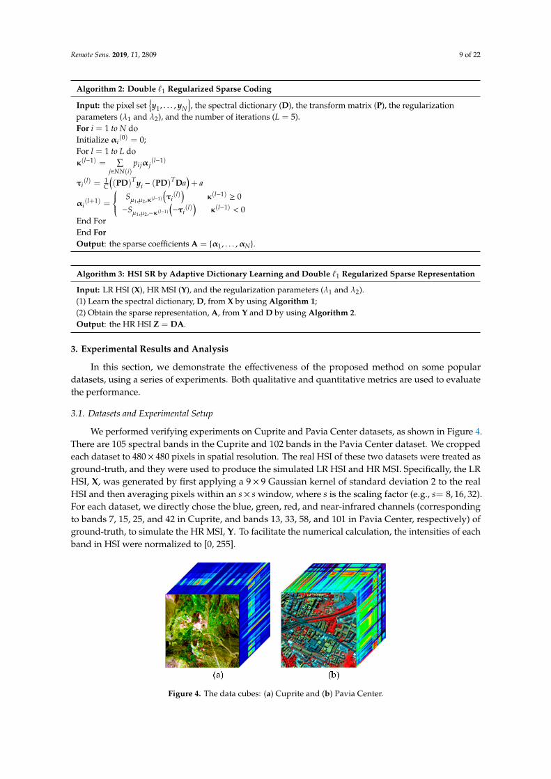
We performed verifying experiments on Cuprite and Pavia Center datasets, as shown in Figure 4.There are 105 spectral bands in the Cuprite and 102 bands in the Pavia Center dataset. We croppedeach dataset to 480× 480 pixels in spatial resolution. The real HSI of these two datasets were treated asground-truth, and they were used to produce the simulated LR HSI and HR MSI. Specifically, the LRHSI, X, was generated by first applying a 9 × 9 Gaussian kernel of standard deviation 2 to the realHSI and then averaging pixels within an s× s window, where s is the scaling factor (e.g., s= 8, 16, 32).For each dataset, we directly chose the blue, green, red, and near-infrared channels (correspondingto bands 7, 15, 25, and 42 in Cuprite, and bands 13, 33, 58, and 101 in Pavia Center, respectively) ofground-truth, to simulate the HR MSI, Y. To facilitate the numerical calculation, the intensities of eachband in HSI were normalized to [0, 255].
Figure 4. The data cubes: (a) Cuprite and (b) Pavia Center.
Remote Sens. 2019, 11, 2809 10 of 22
The proposed method is compared with five representative algorithms: SASFM [32],G-SOMP+ [34], SSR [40], NNSR [38], and SSCSR [39]. To ensure the reliability of the results,we repeat each super resolution method 20 times on the test datasets.
3.2. Quality Metrics
We adopt three quantitative measures for the evaluation: relative dimensionless global error insynthesis (ERGAS) [49], root mean square error (RMSE), and spectral angle mapper (SAM) [50].
The RMSE measures the deviation between the reference HR HSI, R, and the reconstructed HRHSI, Z:
RMSE =
√‖R−Z‖2F
BN(31)
The ERGAS metric [49] calculates the average amount of spectral deviation in each band, as definedbelow:
ERGAS =100
s·
√1B
∑ RMSE(rb, zb)
µrb
(32)
where s is the scaling factor, rb and zb represents the b-th band of R and Z, respectively, and µrb is themean of rb.
At last, we calculated SAM [50], which is defined as the angle between two spectral vectors, rb andzb, averaged over all pixels:
SAM =1N
∑arccos
rbTzb
(rbTrb)
1/2· (zb
Tzb)1/2
(33)
According to the above definition, the smaller the RMSE, ERGAS, and SAM metrics, the better thesuper-resolution performance.
3.3. Performance Comparison of Different Methods
Table 1 shows the average RMSE, ERGAS, and SAM results of the two datasets under differentdownsampling factors by the six compared methods. Our approach outperforms the others in terms ofthe RMSE, ERGAS, and SAM results, which clearly indicates that the adaptive learned dictionary canexploit the underlying structures in the HSI. The double `1 regularized sparse representation illustratesthe superior performance over other competing methods. Thus, these numerical results validate thepower of the proposed model for HSI super-resolution.
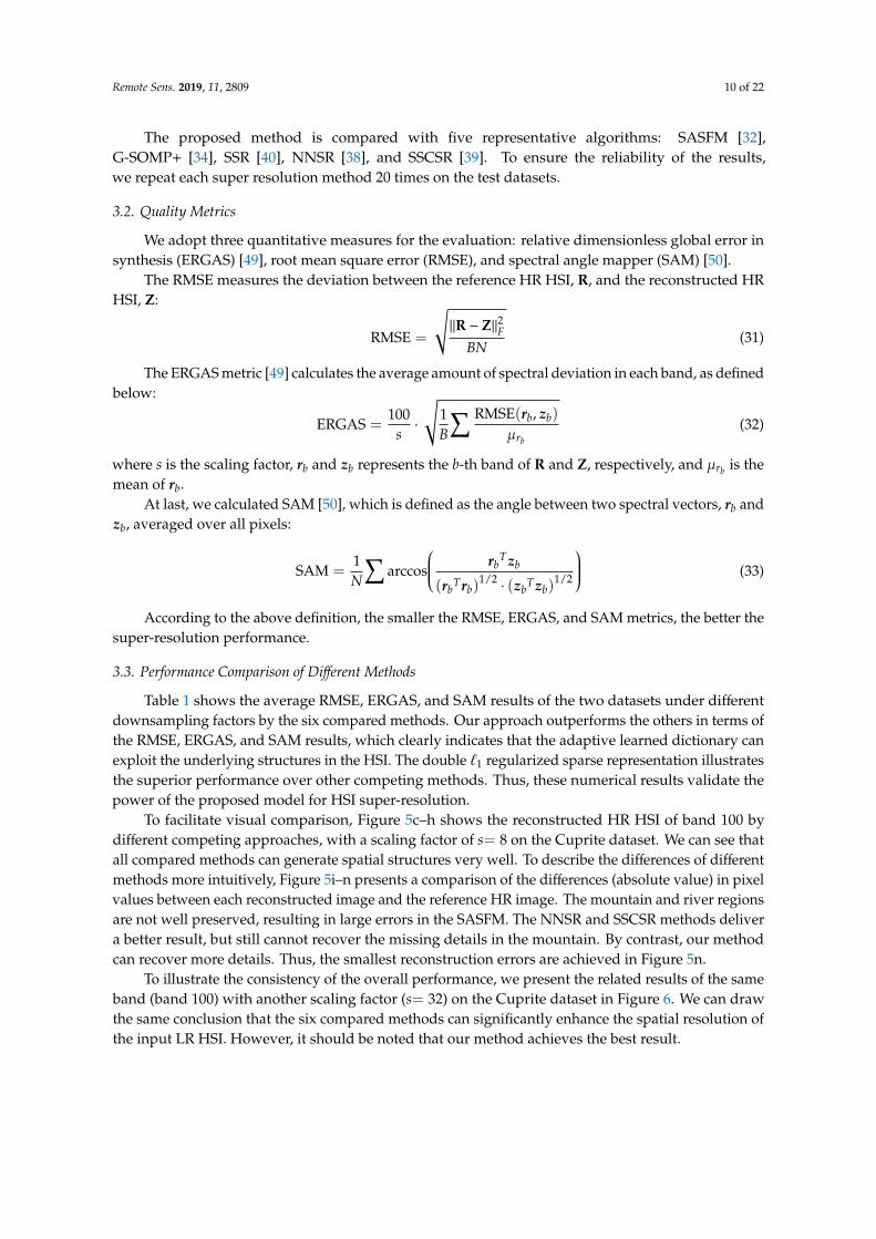
To facilitate visual comparison, Figure 5c–h shows the reconstructed HR HSI of band 100 bydifferent competing approaches, with a scaling factor of s= 8 on the Cuprite dataset. We can see thatall compared methods can generate spatial structures very well. To describe the differences of differentmethods more intuitively, Figure 5i–n presents a comparison of the differences (absolute value) in pixelvalues between each reconstructed image and the reference HR image. The mountain and river regionsare not well preserved, resulting in large errors in the SASFM. The NNSR and SSCSR methods delivera better result, but still cannot recover the missing details in the mountain. By contrast, our methodcan recover more details. Thus, the smallest reconstruction errors are achieved in Figure 5n.
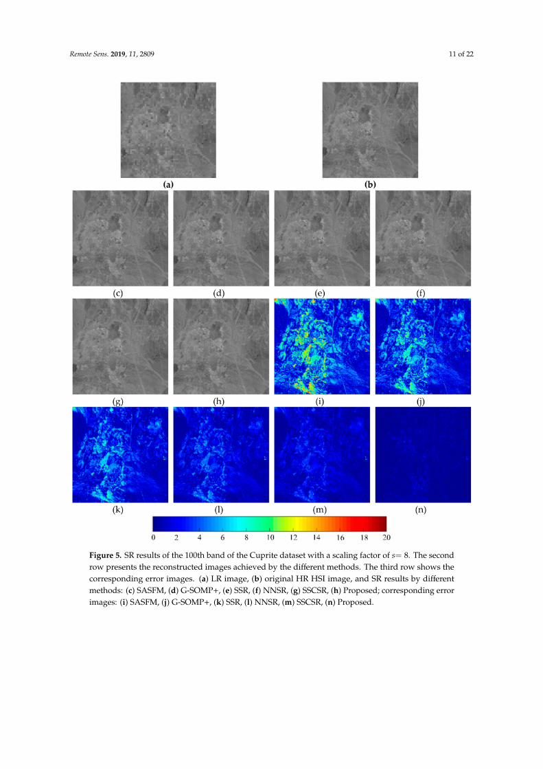
To illustrate the consistency of the overall performance, we present the related results of the sameband (band 100) with another scaling factor (s= 32) on the Cuprite dataset in Figure 6. We can drawthe same conclusion that the six compared methods can significantly enhance the spatial resolution ofthe input LR HSI. However, it should be noted that our method achieves the best result.
Remote Sens. 2019, 11, 2809 11 of 22
Figure 5. SR results of the 100th band of the Cuprite dataset with a scaling factor of s= 8. The secondrow presents the reconstructed images achieved by the different methods. The third row shows thecorresponding error images. (a) LR image, (b) original HR HSI image, and SR results by differentmethods: (c) SASFM, (d) G-SOMP+, (e) SSR, (f) NNSR, (g) SSCSR, (h) Proposed; corresponding errorimages: (i) SASFM, (j) G-SOMP+, (k) SSR, (l) NNSR, (m) SSCSR, (n) Proposed.
Remote Sens. 2019, 11, 2809 12 of 22
Figure 6. SR results of the 100th band of the Cuprite dataset with a scaling factor of s= 32. The secondrow presents the reconstructed images achieved by the different methods. The third row shows thecorresponding error images. (a) LR image, (b) original HR HSI image, and SR results by differentmethods: (c) SASFM, (d) G-SOMP+, (e) SSR, (f) NNSR, (g) SSCSR, (h) Proposed; corresponding errorimages: (i) SASFM, (j) G-SOMP+, (k) SSR, (l) NNSR, (m) SSCSR, (n) Proposed.
Remote Sens. 2019, 11, 2809 13 of 22
Table 1. Quantitative measures by different methods on Cuprite and Pavia Center.
DownsamplingFactor
MethodsCuprite Pavia Center
RMSE ERGAS SAM RMSE ERGAS SAM
s= 8
SASFM 1.0065 0.5987 2.1624 1.8734 0.7003 2.3561G-SOMP+ 0. 8410 0.5683 1.8999 1.5552 0.5826 1.9708
SSR 0.7627 0.5511 1.8239 1.2390 0.5747 1.9089NNSR 0.6373 0.4562 1.6120 1.1537 0.5521 1.8295SSCSR 0.5663 0.3318 1.2278 0.0990 0.5159 1.7566
Proposed 0.4852 0.2961 0.9088 1.0574 0.4975 1.6388
s= 16
SASFM 1.1818 0.3136 1.9852 2.1621 0.3519 2.4395G-SOMP+ 0.9109 0.2796 1.7674 1.7861 0.3009 2.1477
SSR 0.8567 0.2788 1.7585 1.3697 0.2978 2.1344NNSR 0.7629 0.2005 1.5662 1.2790 0.2977 1.9591SSCSR 0.6937 0.1811 1.3039 1.2190 0.2891 1.8889
Proposed 0.5474 0.1695 1.0157 1.1904 0.2837 1.8650
s= 32
SASFM 1.4076 0.1629 2.0011 4.2323 0.3002 4.0387G-SOMP+ 1.1267 0.1436 1.8117 3.8084 0.2511 3.3054
SSR 0.9845 0.1397 1.7546 3.4486 0.2332 2.9203NNSR 0.8393 0.1128 1.4658 2.8099 0.2008 2.5580SSCSR 0.7654 0.1095 1.3267 2.2790 1.1744 2.3016
Proposed 0.6826 0.1015 1.1990 2.1847 0.1575 2.0664
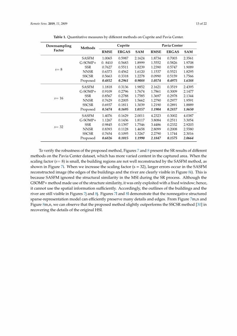
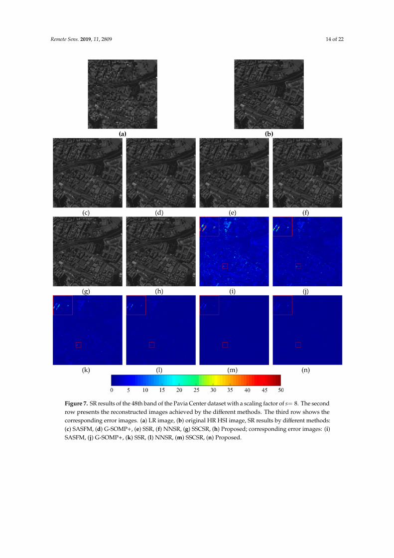
To verify the robustness of the proposed method, Figures 7 and 8 present the SR results of differentmethods on the Pavia Center dataset, which has more varied content in the captured area. When thescaling factor (s= 8) is small, the building regions are not well reconstructed by the SASFM method, asshown in Figure 7i. When we increase the scaling factor (s = 32), larger errors occur in the SASFMreconstructed image (the edges of the buildings and the river are clearly visible in Figure 8i). This isbecause SASFM ignored the structural similarity in the MSI during the SR process. Although theGSOMP+ method made use of the structure similarity, it was only exploited with a fixed window; hence,it cannot use the spatial information sufficiently. Accordingly, the outlines of the buildings and theriver are still visible in Figures 7j and 8j. Figures 7l and 8l demonstrate that the nonnegative structuredsparse-representation model can efficiently preserve many details and edges. From Figure 7m,n andFigure 8m,n, we can observe that the proposed method slightly outperforms the SSCSR method [30] inrecovering the details of the original HSI.
Remote Sens. 2019, 11, 2809 14 of 22
Figure 7. SR results of the 48th band of the Pavia Center dataset with a scaling factor of s= 8. The secondrow presents the reconstructed images achieved by the different methods. The third row shows thecorresponding error images. (a) LR image, (b) original HR HSI image, SR results by different methods:(c) SASFM, (d) G-SOMP+, (e) SSR, (f) NNSR, (g) SSCSR, (h) Proposed; corresponding error images: (i)SASFM, (j) G-SOMP+, (k) SSR, (l) NNSR, (m) SSCSR, (n) Proposed.
Remote Sens. 2019, 11, 2809 15 of 22
Figure 8. SR results of the 94th band of the Pavia Center dataset with scaling factor of s= 32. The secondrow presents the reconstructed images achieved by the different methods. The third row shows thecorresponding error images. (a) LR image, (b) original HR HSI image, SR results by different methods:(c) SASFM, (d) G-SOMP+, (e) SSR, (f) NNSR, (g) SSCSR, (h) Proposed; corresponding error images: (i)SASFM, (j) G-SOMP+, (k) SSR, (l) NNSR, (m) SSCSR, (n) Proposed.
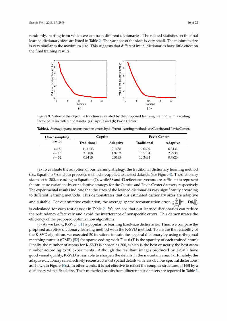
3.4. Effects of the Adaptive Size Dictionary
(1) In Figure 9, we present the values of objective function (10) vs. the iteration times. This provesthat the proposed algorithm terminates in finite steps. The optimal value of the objective functionis achieved after 15 iterations for each dataset. In Algorithm 1, a random dictionary is selected forthe initialization. Thus, further experiments are conducted to evaluate the sensitivity of our learningalgorithm to different starting points. For each dataset, we generate 200 different initial dictionaries
Remote Sens. 2019, 11, 2809 16 of 22
randomly, starting from which we can train different dictionaries. The related statistics on the finallearned dictionary sizes are listed in Table 2. The variance of the sizes is very small. The minimum sizeis very similar to the maximum size. This suggests that different initial dictionaries have little effect onthe final training results.
Figure 9. Value of the objective function evaluated by the proposed learning method with a scalingfactor of 32 on different datasets: (a) Cuprite and (b) Pavia Center.
Table 2. Average sparse reconstruction errors by different learning methods on Cuprite and Pavia Center.
DownsamplingFactor
Cuprite Pavia Center
Traditional Adaptive Traditional Adaptive
s= 8 11.1233 2.1488 19.0409 6.3434s= 16 2.1488 1.9752 15.5154 2.9938s= 32 0.6115 0.5165 10.3444 0.7820
(2) To evaluate the adaption of our learning strategy, the traditional dictionary learning method(i.e., Equation (7)) and our proposed method are applied to the test datasets (see Figure 4). The dictionarysize is set to 300, according to Equation (7), while 38 and 43 reflectance vectors are sufficient to representthe structure variations by our adaptive strategy for the Cuprite and Pavia Center datasets, respectively.The experimental results indicate that the sizes of the learned dictionaries vary significantly accordingto different learning methods. This demonstrates that our estimated dictionary sizes are adaptive
and suitable. For quantitative evaluation, the average sparse reconstruction error, 1n
n∑i=1
∥∥∥xi −Dβi∥∥∥2
2,
is calculated for each test dataset in Table 2. We can see that our learned dictionaries can reducethe redundancy effectively and avoid the interference of nonspecific errors. This demonstrates theefficiency of the proposed optimization algorithms.
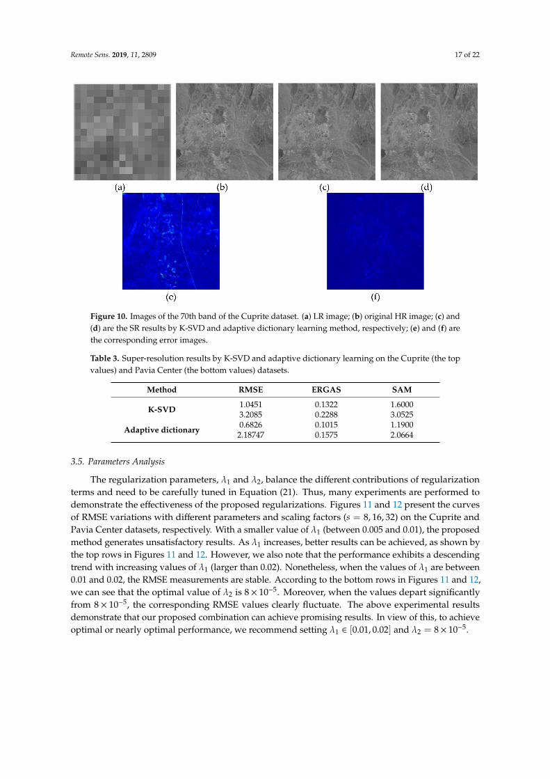
(3) As we know, K-SVD [51] is popular for learning fixed-size dictionaries. Thus, we compare theproposed adaptive dictionary learning method with the K-SVD method. To ensure the reliability ofthe K-SVD algorithm, we executed 50 iterations to train the spectral dictionary by using orthogonalmatching pursuit (OMP) [52] for sparse coding with T = 6 (T is the sparsity of each trained atom).Finally, the number of atoms for K-SVD is chosen as 300, which is the best or nearly the best atomnumber according to 20 experiments. Although the resultant images produced by K-SVD havegood visual quality, K-SVD is less able to sharpen the details in the mountain area. Fortunately, theadaptive dictionary can effectively reconstruct most spatial details with less obvious spectral distortions,as shown in Figure 10e,f. In other words, it is not effective to reflect the complex structures of HSI by adictionary with a fixed size. Their numerical results from different test datasets are reported in Table 3.
Remote Sens. 2019, 11, 2809 17 of 22
Figure 10. Images of the 70th band of the Cuprite dataset. (a) LR image; (b) original HR image; (c) and(d) are the SR results by K-SVD and adaptive dictionary learning method, respectively; (e) and (f) arethe corresponding error images.
Table 3. Super-resolution results by K-SVD and adaptive dictionary learning on the Cuprite (the topvalues) and Pavia Center (the bottom values) datasets.
Method RMSE ERGAS SAM
K-SVD 1.04513.2085
0.13220.2288
1.60003.0525
Adaptive dictionary 0.68262.18747
0.10150.1575
1.19002.0664
3.5. Parameters Analysis
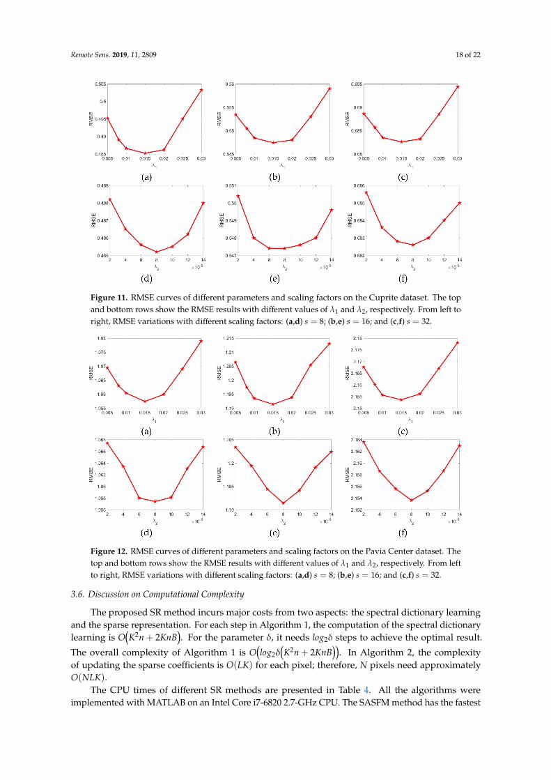
The regularization parameters, λ1 and λ2, balance the different contributions of regularizationterms and need to be carefully tuned in Equation (21). Thus, many experiments are performed todemonstrate the effectiveness of the proposed regularizations. Figures 11 and 12 present the curvesof RMSE variations with different parameters and scaling factors (s = 8, 16, 32) on the Cuprite andPavia Center datasets, respectively. With a smaller value of λ1 (between 0.005 and 0.01), the proposedmethod generates unsatisfactory results. As λ1 increases, better results can be achieved, as shown bythe top rows in Figures 11 and 12. However, we also note that the performance exhibits a descendingtrend with increasing values of λ1 (larger than 0.02). Nonetheless, when the values of λ1 are between0.01 and 0.02, the RMSE measurements are stable. According to the bottom rows in Figures 11 and 12,we can see that the optimal value of λ2 is 8 × 10⁻⁵. Moreover, when the values depart significantlyfrom 8 × 10⁻⁵, the corresponding RMSE values clearly fluctuate. The above experimental resultsdemonstrate that our proposed combination can achieve promising results. In view of this, to achieveoptimal or nearly optimal performance, we recommend setting λ1 ∈ [0.01, 0.02] and λ2 = 8× 10⁻⁵.
Remote Sens. 2019, 11, 2809 18 of 22
Figure 11. RMSE curves of different parameters and scaling factors on the Cuprite dataset. The topand bottom rows show the RMSE results with different values of λ1 and λ2, respectively. From left toright, RMSE variations with different scaling factors: (a,d) s = 8; (b,e) s = 16; and (c,f) s = 32.
Figure 12. RMSE curves of different parameters and scaling factors on the Pavia Center dataset. Thetop and bottom rows show the RMSE results with different values of λ1 and λ2, respectively. From leftto right, RMSE variations with different scaling factors: (a,d) s = 8; (b,e) s = 16; and (c,f) s = 32.
3.6. Discussion on Computational Complexity
The proposed SR method incurs major costs from two aspects: the spectral dictionary learningand the sparse representation. For each step in Algorithm 1, the computation of the spectral dictionarylearning is O
(K2n + 2KnB
). For the parameter δ, it needs log2δ steps to achieve the optimal result.
The overall complexity of Algorithm 1 is O(log2δ
(K2n + 2KnB
)). In Algorithm 2, the complexity
of updating the sparse coefficients is O(LK) for each pixel; therefore, N pixels need approximatelyO(NLK).
The CPU times of different SR methods are presented in Table 4. All the algorithms wereimplemented with MATLAB on an Intel Core i7-6820 2.7-GHz CPU. The SASFM method has the fastest
Remote Sens. 2019, 11, 2809 19 of 22
running time through the sparse coding technique of OMP [52]. The SSR and SSCSR methods havea long processing time due to the clustering-based sparse representation framework. Our proposedmethod runs quite slowly and requires approximately 5 min. In the future, we can expect to speed upthe proposed algorithm by using a graphics-processing unit.
Table 4. Average running time (seconds) of the compared methods on the simulated datasets with ascaling factor of 32.
Method SASFM G-SOMP+ SSR NNSR SSCSR Proposed
Time 11 235 579 146 723 276
4. Discussion
Compared to other methods, the proposed method achieves a superior SR performance. There aremainly two reasons why. First, the adaptive dictionary can represent different variations reasonablycompared with traditional dictionary learning methods. Second, the nonlocal similarities of the sparsecoefficients are exploited to improve the HSI SR quality.
From the parameter analysis, we can find that the RMSE stay relatively stable, without anyincremental performance, when the parameters are set to the recommended values (see Figures 11and 12). In other words, the performance of our proposed method is robust. From the comparison ofthe execution time, we observe that the proposed model is not computationally efficient (see Table 4).However, our method could achieve better performance in comparison with other methods on the twohyperspectral datasets. In light of this, it will be interesting to design an architecture with multicoreCPU [53], to optimize the execution time.
5. Conclusions
This paper proposed a new and effective method for HSI super-resolution based on sparserepresentation. There are two distinctive features of the proposed method. On the one hand,an adaptive learning strategy is used to learn a spectral dictionary, which represents different contentand features reasonably. On the other hand, double `1 regularized constraints are employed tocharacterize the similarities of the sparse coefficients, to improve the HSI SR quality. Extensiveexperimental results from two popular HSI datasets validate the superior performance of the proposedmethod over other competitive methods. The experiments of the parameters demonstrate the robustnessof the proposed method.
In the future, we can combine the tensor model [54] and the shape-adaptive technique [55,56]to explore the spatial–spectral information adaptively and sufficiently. Deep-learning approacheshave recently gained great attention in many fields [57–64]. It will be a new task to design a deeparchitecture to improve the performance of the HSI SR.
Author Contributions: Experiments and writing, S.T.; supervision, Y.X.; review and editing, L.S. and L.H.
Funding: This research was supported in part by the Fundamental Research Funds for the Central Universities(Grant No. LGZD201702, LGYB201807), the Natural Science Foundation of Jiangsu Province (Grant No. BK20171074and BK 20150792), and the National Natural Science Foundation of China (Grant No. 61702269 and 61971233).
Acknowledgments: The authors would like to thank the Assistant Editor who handled our paper and theanonymous reviewers for providing help comments that significantly helped us improve the technical quality andpresentation of our paper.
Conflicts of Interest: The authors declare no conflicts of interest.
References
1. Sun, L.; Zhan, T.; Wu, Z.; Xiao, L.; Jeon, B. Hyperspectral mixed denoising via spectral difference-inducedtotal variation and low-rank approximation. Remote Sens. 2018, 10, 1956. [CrossRef]
Remote Sens. 2019, 11, 2809 20 of 22
2. Sun, L.; Jeon, B.; Bushra, N.S.; Zheng, Y.H.; Wu, Z.B.; Xiao, L. Fast superpixel based subspace low ranklearning method for hyperspectral denoising. IEEE Access. 2018, 6, 12031–12043. [CrossRef]
3. Gao, H.; Yang, Y.; Li, C.; Zhou, H.; Qu, X. Joint Alternate Small Convolution and Feature Reuse forHyperspectral Image Classification. ISPRS Int. J. Geo Inf. 2018, 7, 349. [CrossRef]
4. Sun, L.; Ma, C.; Chen, Y.; Zheng, Y.; Shim, H.J.; Wu, Z.; Jeon, B. Low Rank Component Induced Spatial-spectralKernel Method for Hyperspectral Image Classification; IEEE: New York, NY, USA, 2019; pp. 1–14.
5. Van Nguyen, H.; Banerjee, A.; Chellappa, R. Tracking via Object Reflectance Using a Hyperspectral VideoCamera. In Proceedings of the IEEE Computer Society Conference on Computer Vision and PatternRecognition—Workshops, San Francisco, CA, USA, 13–18 June 2010; pp. 44–51.
6. Uzair, M.; Mahmood, A.; Mian, A. Hyperspectral Face Recognition using 3D-DCT and Partial Least Squares.In Proceedings of the British Machine Vision Conference, Bristol, UK, 9–13 September 2013; p. 57.
7. Yang, J.; Jiang, Z.; Hao, S.; Zhang, H. Higher Order Support Vector Random Fields for Hyperspectral ImageClassification. ISPRS Int. J. Geo Inf. 2018, 7, 19. [CrossRef]
8. Wang, Y.; Chen, X.; Han, Z.; He, S. Hyperspectral Image Super-Resolution via Nonlocal Low-Rank TensorApproximation and Total Variation Regularization. Remote. Sens. 2017, 9, 1286. [CrossRef]
9. Tang, S.; Xiao, L.; Huang, W.; Liu, P.; Wu, H. Pan-sharpening using 2D CCA. Remote Sens. Lett. 2015, 6, 341–350.[CrossRef]
10. Tu, T.-M.; Huang, P.; Hung, C.-L.; Chang, C.-P. A Fast Intensity–Hue–Saturation Fusion Technique WithSpectral Adjustment for IKONOS Imagery. IEEE Geosci. Remote. Sens. Lett. 2004, 1, 309–312. [CrossRef]
11. Liu, P.; Xiao, L. A Novel Generalized Intensity-Hue-Saturation (GIHS) Based Pan-Sharpening Method WithVariational Hessian Transferring. IEEE Access 2018, 6, 46751–46761. [CrossRef]
12. El-Mezouar, M.C.; Kpalma, K.; Taleb, N.; Ronsin, J. A pan-sharpening based on the non-subsampledcontourlet transform: application to WorldView-2 imagery. IEEE J. Sel. Top. Appl. Earth Obs. Remote Sens.2014, 7, 1806–1815. [CrossRef]
13. Garzelli, A.; Aiazzi, B.; Alparone, L.; Lolli, S.; Vivone, G. Multispectral pansharpening with radiativetransfer-based detail-injection modeling for preserving changes in vegetation cover by Andrea. Remote Sens.2018, 10, 1308. [CrossRef]
14. Li, S.; Yang, B. A new pan-sharpening method using a compressed sensing technique. IEEE Trans. Geosci.Remote Sens. 2010, 49, 738–746. [CrossRef]
15. Liu, P.; Xiao, L.; Li, T. A Variational Pan-Sharpening Method Based on Spatial Fractional-Order Geometryand Spectral–Spatial Low-Rank Priors. IEEE Trans. Geosci. Remote. Sens. 2018, 56, 1788–1802. [CrossRef]
16. Tang, S. Pansharpening via sparse regression. Opt. Eng. 2017, 56, 1. [CrossRef]17. Yokoya, N.; Grohnfeldt, C.; Chanussot, J. Hyperspectral and Multispectral Data Fusion: A comparative
review of the recent literature. IEEE Geosci. Remote. Sens. Mag. 2017, 5, 29–56. [CrossRef]18. Veganzones, M.A.; Simoes, M.; Licciardi, G.; Yokoya, N.; Bioucas-Dias, J.M.; Chanussot, J. Hyperspectral
super-resolution of locally low rank images from complementary multisource data. IEEE Trans. Image Proc.2015, 25, 274–288. [CrossRef]
19. Yokoya, N.; Yairi, T.; Iwasaki, A. Coupled nonnegative matrix factorization unmixing for hyperspectral andmultispectral data fusion. IEEE Geosci. Remote Sens. 2011, 50, 528–537. [CrossRef]
20. Lee, D.D.; Seung, H.S. Learning the parts of objects by non-negative matrix factorization. Nature1999, 401, 788–791. [CrossRef]
21. Lee, D.D.; Seung, H.S. Algorithms for Non-Negative Matrix Factorization. In Advances in Neural InformationProcessing Systems; Michael, I.J., Yann, L.C., Sara, A.S., Eds.; MIT Press: Cambridge, MA, USA, 2001;pp. 556–562.
22. Bendoumi, M.A.; He, M.; Mei, S. Hyperspectral Image Resolution Enhancement Using High-ResolutionMultispectral Image Based on Spectral Unmixing. IEEE Trans. Geosci. Remote. Sens. 2014, 52, 6574–6583.[CrossRef]
23. Keshava, N.; Mustard, J.F. Spectral unmixing. IEEE Signal Process Mag. 2002, 19, 44–57.24. Iordache, M.-D.; Bioucas-Dias, J.M.; Plaza, A. Sparse Unmixing of Hyperspectral Data. IEEE Trans. Geosci.
Remote. Sens. 2011, 49, 2014–2039. [CrossRef]25. Kawakami, R.; Matsushita, Y.; Wright, J.; Ben-Ezra, M.; Tai, Y.-W.; Ikeuchi, K. High-Resolution Hyperspectral
Imaging via Matrix Factorization. In Proceedings of the IEEE Conference on Computer Vision and PatternRecognition, Colorado Springs, CO, USA, 20–25 June 2011; pp. 2329–2336.
Remote Sens. 2019, 11, 2809 21 of 22
26. Li, S.; Dian, R.; Fang, L.; Bioucas-Dias, J.M. Fusing Hyperspectral and Multispectral Images via CoupledSparse Tensor Factorization. IEEE Trans. Image Process. 2018, 27, 4118–4130. [CrossRef] [PubMed]
27. Dian, R.; Fang, L.; Li, S. Hyperspectral Image Super-Resolution via Non-local Sparse Tensor Factorization.In Proceedings of the IEEE Conference on Computer Vision and Pattern Recognition, Honolulu, HI, USA,21–26 July 2017 ; pp. 3862–3871.
28. Wei, Q.; Bioucas-Dias, J.; Dobigeon, N.; Tourneret, J.Y. Hyperspectral and multispectral image fusion basedon a sparse representation. IEEE Trans. Geosci. Remote Sens. 2015, 53, 3658–3668. [CrossRef]
29. Akhtar, N.; Shafait, F.; Mian, A. Bayesian Sparse Representation for Hyperspectral Image Super Resolution.In Proceedings of the IEEE Conference on Computer Vision and Pattern Recognition, Boston, MA, USA,8–12 June 2015; pp. 3631–3640.
30. Yi, C.; Zhao, Y.Q.; Chan, J.C.W. Hyperspectral image super-resolution based on spatial and spectral correlationrusion. IEEE Trans. Geosci. Remote Sens. 2018, 56, 4165–4177. [CrossRef]
31. Zhang, L.; Wei, W.; Bai, C.; Gao, Y.; Zhang, Y. Exploiting Clustering Manifold Structure for HyperspectralImagery Super-Resolution. IEEE Trans. Image Process. 2018, 27, 5969–5982. [CrossRef] [PubMed]
32. Huang, B.; Song, H.; Cui, H.; Peng, J.; Xu, Z. Spatial and spectral image fusion using sparse matrixfactorization. IEEE Trans. Geosci. Remote Sens. 2013, 52, 1693–1704. [CrossRef]
33. Grohnfeldt, C.; Zhu, X.X.; Bamler, R. Jointly Sparse Fusion of Hyperspectral and Multispectral Imagery.In Proceedings of the 2013 IEEE International Geoscience and Remote Sensing Symposium, Melbourne,Australia, 21–26 July 2013; pp. 4090–4093.
34. Akhtar, N.; Shafait, F.; Mian, A. Sparse Spatio-Spectral Representation for Hyper-Spectral ImageSuper-Resolution. In Proceedings of the European Conference on Computer Vision (ECCV), Zurich,Switzerland, 6–12 September 2014; pp. 63–78.
35. Liang, J.; Zhang, Y.; Mei, S. Hyperspectral and Multispectral Image Fusion using Dual-Source LocalizedDictionary Pair. In Proceedings of the International Symposium on Intelligent Signal Processing andCommunication Systems, Xiamen, Fujian, China, 6–9 November 2017; pp. 261–264.
36. Lanaras, C.; Baltsavias, E.; Schindler, K.; Charis, L.; Emmanuel, B.; Konrad, S. Hyperspectral Super-Resolutionby Coupled Spectral Unmixing. In Proceedings of the IEEE International Conference on Computer Vision,Venice, Italy, 22–29 October 2015; pp. 3586–3594.
37. Lanaras, C.; Baltsavias, E.; Schindler, K. Hyperspectral Super-Resolution with Spectral Unmixing Constraints.Remote. Sens. 2017, 9, 1196. [CrossRef]
38. Dong, W.; Fu, F.; Shi, G.; Cao, X.; Wu, J.; Li, G.; Li, X. Hyperspectral Image Super-Resolution via Non-NegativeStructured Sparse Representation. IEEE Trans. Image Process. 2016, 25, 2337–2352. [CrossRef]
39. Han, X.-H.; Shi, B.; Zheng, Y. Self-Similarity Constrained Sparse Representation for Hyperspectral ImageSuper-Resolution. IEEE Trans. Image Process. 2018, 27, 5625–5637. [CrossRef]
40. Fang, L.Y.; Zhuo, H.J.; Li, S.T. Super-resolution of hyperspectral image via superpixel-based sparserepresentation. Neurocomputing 2018, 273, 171–177. [CrossRef]
41. Buades, A.; Coll, B.; Morel, J.-M. A Non-Local Algorithm for Image Denoising. In Proceedings of the 2005IEEE Computer Society Conference on Computer Vision and Pattern Recognition (CVPR 05), San Diego, CA,USA, 20–25 June 2005; 2, pp. 60–65.
42. Glasner, D.; Bagon, S.; Irani, M. Super-resolution from a single image. In Proceedings of the IEEE 12thInternational Conference on Computer Vision, Kyoto, Japan, 29 September–2 October 2009; pp. 349–356.
43. Cotter, S.; Rao, B.; Engan, K.; Kreutz-Delgado, K. Sparse solutions to linear inverse problems with multiplemeasurement vectors. IEEE Trans. Signal Process. 2005, 53, 2477–2488. [CrossRef]
44. Lu, C.; Shi, J.; Jia, J. Scale adaptive dictionary learning. IEEE Trans. Image Process. 2013, 23, 837–847.[CrossRef] [PubMed]
45. Aharon, M.; Elad, M. Sparse and redundant modeling of image content using an image-signature-dictionary.SIAM J. Imaging Sci. 2008, 1, 228–247. [CrossRef]
46. Beck, A.; Teboulle, M. A Fast Iterative Shrinkage-Thresholding Algorithm for Linear Inverse Problems.SIAM J. Imaging Sci. 2009, 2, 183–202. [CrossRef]
47. Tang, S.; Zhou, N. Local Similarity Regularized Sparse Representation for Hyperspectral ImageSuper-Resolution. IEEE International Geoscience and Remote Sensing Symposium, Valencia, Spain, 21–29 July2018; pp. 5120–5123.
Remote Sens. 2019, 11, 2809 22 of 22
48. Daubechies, I.; Defrise, M.; De Mol, C. An iterative thresholding algorithm for linear inverse problems witha sparsity constraint. Commun. Pure Appl. Math. 2004, 57, 1413–1457. [CrossRef]
49. Wald, L.; Ranchin, T.; Mangolini, M. Fusion of satellite images of different spatial resolutions: assessing thequality of resulting images. Photogramm. Eng. Remote Sens. 1997, 63, 691–699.
50. Alparone, L.; Wald, L.; Chanussot, J.; Thomas, C.; Gamba, P.; Bruce, L. Comparison of PansharpeningAlgorithms: Outcome of the 2006 GRS-S Data-Fusion Contest. IEEE Trans. Geosci. Remote. Sens.2007, 45, 3012–3021. [CrossRef]
51. Aharon, M.; Elad, M.; Bruckstein, Y. K-SVD: An algorithm for designing of overcomplete dictionaries forsparse representation. IEEE Trans. Signal Process 2006, 54, 4311–4322. [CrossRef]
52. Pati, Y.C.; Rezaiifar, R.; Krishnaprasad, P.S. Orthogonal Matching Pursuit: Recursive Function Approximationwith Applications to Wavelet Decomposition. In Proceedings of the 27th Asilomar Conference on Signals,Systems and Computers, Pacific Grove, CA, USA, 1–3 November 1993; pp. 40–44.
53. Jiang, Y.; Zhao, M.; Hu, C.; He, L.; Bai, H.; Wang, J. A parallel FP-growth algorithm on World Ocean Atlasdata with multi-core CPU. J. Supercomput. 2019, 75, 732–745. [CrossRef]
54. Kolda, T.G.; Bader, B.W. Tensor Decompositions and Applications. SIAM Rev. 2009, 51, 455–500. [CrossRef]55. Foi, A.; Katkovnik, V.; Egiazarian, K. Pointwise shape-adaptive DCT for high-quality denoising and
deblocking of grayscale and color images. IEEE Trans. Image Process. 2007, 16, 1395–1411. [CrossRef]56. Müller, H.-G.; Fan, J.; Gijbels, I. Local Polynomial Modeling and Its Applications. J. Am. Stat. Assoc. 1998, 93, 835.
[CrossRef]57. Tu, Y.; Lin, Y.; Wang, J.; Kim, J.U. Semi-supervised learning with generative adversarial networks on digital
signal modulation classification. Comput. Mater. Contin. 2018, 55, 243–254.58. Meng, R.; Rice, S.G.; Wang, J.; Sun, X. A fusion steganographic algorithm based on faster R-CNN.
Comput. Mater. Contin. 2018, 55, 1–16.59. Long, M.; Zeng, Y. Detecting Iris Liveness with Batch Normalized Convolutional Neural Network.
Comput. Mater. Contin. 2019, 58, 493–504. [CrossRef]60. He, S.; Li, Z.; Tang, Y.; Liao, Z.; Wang, J.; Kim, H.J. Parameters compressing in deep learning. Comput. Mater.
Contin. 2019, 62, 1–16.61. Song, Y.; Yang, G.; Xie, H.; Zhang, D.; Xingming, S. Residual domain dictionary learning for compressed
sensing video recovery. Multimed. Tools Appl. 2017, 76, 10083–10096. [CrossRef]62. Zeng, D.; Dai, Y.; Li, F.; Wang, J.; Sangaiah, A.K. Aspect based sentiment analysis by a linguistically
regularized CNN with gated mechanism. J. Intell. Fuzzy Syst. 2019, 36, 3971–3980. [CrossRef]63. Zhang, J.; Jin, X.; Sun, J.; Wang, J.; Sangaiah, A.K. Spatial and semantic convolutional features for robust
visual object tracking. Multimedia Tools Appl. 2018, 1, 1–21. [CrossRef]64. Zhou, S.; Ke, M.; Luo, P. Multi-camera transfer GAN for person re-dentification. J. Vis. Commun. Image R.
2019, 59, 393–400. [CrossRef]
© 2019 by the authors. Licensee MDPI, Basel, Switzerland. This article is an open accessarticle distributed under the terms and conditions of the Creative Commons Attribution(CC BY) license (http://creativecommons.org/licenses/by/4.0/).


