Repeated measurements on permanent plots using local variability sampling for monitoring soil cover

Available online at www.sciencedirect.com

) 75–88www.elsevier.com/locate/catena

Catena 73 (2008

Repeated measurements on permanent plots using local variabilitysampling for monitoring soil cover

G. Wang a, G. Gertner a,⁎, A.B. Anderson b, H. Howard b

a W503 Turner Hall, 1102 S. Goodwin Ave., University of IL, Urbana, IL 61801, USAb US Army Corps of Engineers, CERL, P.O. Box 9005, Champaign, IL, USA

Received 2 February 2007; received in revised form 22 August 2007; accepted 12 September 2007

Abstract

On US military installations, training activities such as vehicle use disturb ground and vegetation cover of landscapes, and increase potentialrainfall runoff and soil erosion. In order to sustain training lands, soil erosion is of major concern. Thus there is a need for sampling designs tomonitor degradation and recovery of land conditions. Traditionally, permanent plots are used to obtain the change of land conditions. However, thepermanent plots often provide less information over time in characterizing the land conditions because of the fixed number and locations of plots.In this paper, we analyzed the sufficiency of a permanent plot sample and developed a method to improve the re-measurements of the permanentplots over time for a monitoring system of soil erosion based on spatial and temporal variability of a random function. We first applied a localvariability based sampling method to generate reference samples that have sampling distances varying spatially and temporally to monitor a soilerosion relevant cover factor for an installation, Fort Riley, USA. Then, we compared a permanent sample with the reference samples annuallyover 13 years to determine additional sampling in the areas with high variability and temporarily suspending measurements of the permanent plotsin the areas with low variability. The local variability based sampling provides estimates of local variability of the cover factor and thus is morecost-efficient than random sampling. By comparison with a reference samples, the re-measurements obtained should more accurately characterizethe dynamics of the land conditions.© 2007 Elsevier B.V. All rights reserved.

Keywords: Remote sensing; Sampling design; Soil erosion cover factor; Spatial variability

1. Introduction

On the US military installations, training activities such asvehicle use disturb ground and vegetation cover of landscapes,and increase potential rainfall runoff and soil erosion. In order tosustain training lands, soil erosion is of major concern. Thusthere is a need for sampling designs to monitor land conditionsin order to plan training activities. Traditionally, permanentplots have been widely used for monitoring land conditions onUS military installations. Generally, the monitoring programsbased on permanent plots are designed to characterize landconditions and provide a good representation of land conditions.Even if the representation is initially good, the performance of amonitoring program based on permanent plots might degradethrough time. The reason is because the military activities are

⁎ Corresponding author. Fax: +1 217 244 3219.E-mail address: [email protected] (G. Gertner).

0341-8162/$ - see front matter © 2007 Elsevier B.V. All rights reserved.doi:10.1016/j.catena.2007.09.005

unevenly distributed in both space and time, which leads to thespatial and temporal changes of global and local variability ofland conditions. In some areas the spatial variability increasesdue to continuously high intensity of the activities, while inother areas, the spatial variability decreases because noactivities take place and ground and canopy cover recovers.This implies that the sampling design should vary in terms ofthe grid spacing— sampling distance over both space and time.Thus, there is a need to design optimal samples that havevariable sampling distances over space and time. On the otherhand, if the permanent plots are used to monitor the changes ofland conditions, it is necessary to add temporary sample plots inthe high variation area and temporally suspend some permanentplots for re-measurements in the low variation areas.

In sampling, there are two distinct frameworks: design-basedinference and model-based inference. Thompson (1992)discussed the differences between them. In design-basedapproach, values of a variable are regarded as fixed quantities

mailto:[email protected]

http://dx.doi.org/10.1016/j.catena.2007.09.005

76 G. Wang et al. / Catena 73 (2008) 75–88

and the selection probabilities in sampling are used indetermining the expectation. In a model-based approach, thevalues are considered to be realizations of a random functionconsisting of random variables and the estimator is determinedbased on joint distribution of the random variables. Brus and deGruijter (1997) and Laslett et al. (1997) further discussed andcompared these two approaches, and provided some sugges-tions for their applications.

An optimal sample size can be defined as the number of plotsthat minimizes cost given a desired precision of an estimate. Asa model-based framework, simple random sampling that isbased on global variation of a variable aims at optimization ofsampling design at a global level. This method is widely used todesign a permanent sample (Thompson, 1992), but, it oftenleads to a larger sample and duplication of information becausesome plots are too close (Curran, 1988). Compared to simplerandom sampling, stratified sampling can increase the cost-efficiency by taking the within stratum variances into account(Thompson, 1992). However, the traditional methods neglectspatial autocorrelation of random variables and spatial crosscorrelation between them and therefore, they result in thesampling designs that are not optimal (Curran, 1988).

In 1980s', spatial correlation or spatial variability basedmethods were used for sampling designs of natural resource andenvironmental systems (Burgess et al., 1981; McBratney et al.,1981; McBratney and Webster, 1981, 1983a,b; Atkinson et al.,1992, 1994). These methods assume a regionalized variabletheory (Matheron, 1963, 1971) and include kriging variancebased sampling designs for a single variable and cokrigingvariance based sampling designs in the framework of multiplevariables. The methods result in sampling designs that ensuresystematic and neighboring sample points are as far from oneanother as is practical for a fixed sample size and area. Thisminimizes the duplication of information and is more cost-effective than traditional methods for sampling (Curran andWilliamson, 1986; Curran, 1988).

For sampling design using geostatistical methods, furtherenhancements and new developments have been reported. Brusand Heuvelink (2007) used the spatially averaged universalkriging variance for optimization of sample patterns for envi-ronmental variables by incorporating trend estimation error aswell as spatial interpolation error related to regression residuals.Hengl et al. (2003) evaluated spreading of observations in bothfeature and geographical spaces as a key to sampling optimi-zation for spatial prediction by correlation with auxiliary maps.They compared several sampling strategies and suggested thatan equal range stratification design was a good compromisebetween accurate regression model estimation and minimizationof spatial autocorrelation of residuals.

Furthermore, Van Groenigen and Stein (1998) and Steinet al. (1998) presented a spatial simulated annealing method tooptimize sampling schemes. Using this method, samplingconstraints and previous observations were taken into account.The minimization of the mean of shortest distances was used tospatially spreading the sample points, and the Warrick andMyers' (1987) criterion was applied to optimize the fit of therealized distribution of point pairs for the experimental

semivariogram to an a priori defined, idea distribution. Thismethod was also applied in the studies by Van Groenigen et al.(1999) and Stein and Ettema (2003) and in which krigingvariance and spatial simulated annealing were combined foroptimization of sampling designs.

Spatial variability of a variable can be divided into globaland local variability. Global spatial variability is a general trendof variation of a variable over space. Local spatial variability isrelated to locations and can be defined as the variation of thevariable within a location relevant neighborhood, and isdetermined by the data values in addition to spatial configura-tion of the data locations within the neighborhood. Neglectingthe global and local spatial variability may lead to higher costfor the sampling design and larger errors and uncertainty inestimates (Curran, 1988; Curran and Atkinson, 1998). In thegeostatistical methods mentioned above, the kriging or cokri-ging variances are calculated based on semivariograms thatquantify global spatial variability of variables or the residuals ofregression models used for predicting the variables and thespatial configuration of sample data locations, but are not basedon the sample data values of the variables themselves or theirresiduals. Therefore, the sampling distances of the samples fromthe methods are only globally optimal but not for local areas.

Wang et al. (2005) investigated uncertainties of samplingdesigns due to the errors in estimation of semivariograms. Wanget al. (2007) modified the sampling procedure by first stratifyinga study area into homogeneous strata and then carrying outcokriging variance based sampling design for each stratum.This modification increased the sampling and mapping cost-efficiency by taking the between and within strata variabilityinto account. Anderson et al. (2006) further proposed a localvariability based sampling design method using a conditionalco-simulation with remotely sensed data by taking into accountboth global and local variability of the variables. This methodtheoretically can lead to a sampling design with variablesampling distances that are optimal at the local and globallevels. Compared to simple random sampling, the localvariability based sampling greatly reduced the number of thesampled plots and increased the cost-efficiency for sampling.The objective of this study is to analyze the sufficiency of apermanent plot sample and develop a method to improve the re-measurements of the permanent plots over time for a monitoringsystem of soil erosion based on spatial and temporal variabilityof a random function. In addition, this study will furtherdemonstrate the validation of the local variability basedsampling method in a new study area.

2. Materials and methods

2.1. Study area and data sets

This study was carried out at Fort Riley, located innortheastern Kansas, USA. This installation has an area of41,154 ha. It is located in the Bluestem Prairie region and ischaracterized by rolling plains and dissected by stream valleys.Tall grasses dominate this area and wood and shrub lands occurmainly in the stream valleys (in the left of Fig. 1) (Althoff et al.,

Fig. 1. Study area, land cover categories, permanent sample plots established in 1989 and cover factor values for Fort Riley.

77G. Wang et al. / Catena 73 (2008) 75–88

2005). For more than twenty years, a variety of military trainingactivities including field maneuvers, combat vehicle operations,mortar and artillery fire, and small-arms fire, have taken place atFort Riley. These activities have affected the ecosystemprocesses, including disturbing ground and vegetation cover;increasing soil erosion; changing plant composition, vegetationstructures, habitats and biodiversity; and landscape fragmenta-tion. Thus, a sampling design is needed to monitor the dynamicsof the ecosystems processes. This study deals with the samplingdesigns to map and monitor the dynamics of soil erosion.

In the USA, soil erosion is usually predicted using aUniversal Soil Loss Equation (USLE) (Wischmeier and Smith,1978) or Revised USLE (Renard et al., 1997). For a specific andrelatively small area, soil erosion dynamics is mainly controlledby ground cover and vegetation cover. In this equation, aground and vegetation cover factor, simply called cover factorC, is defined as the ratio of soil loss from an area with specifiedcover. This factor reflects the effect of ground and vegetationcover on the reduction of soil loss by reducing sedimentdetachment and runoff. In the revised USLE, this factor dependson canopy cover, ground cover, surface roughness, and soilmoisture. In this study, this factor was defined as functions ofground cover, canopy cover and minimum rain drop height fromcanopy to the ground according to the original USLE and

calculated using the empirical equations (Wischmeier andSmith, 1978).

To collect ground sample data required to predict soil loss atFort Riley, 154 permanent plots with fixed locations wereinstalled in the summer of 1989 using a stratified randomdesign. The strata were defined based on vegetation and soiltypes (in the right of Fig. 1). The permanent plots have been re-measured annually during summers until 2001. The methodused for the sampling and data collection is called the Rangeand Training Land Assessment (RTLA) (formerly called theLand Condition Trend Analysis (LCTA)) plot inventory (Taziket al., 1992). The permanent plots had a width of 6 m and alength of 100 m. A 100 m line transect was located in the centerof each plot. Ground cover and canopy cover were recorded bythe point intercept method as described by Diersing et al.(1992), that is, at 1 m intervals (0.5 m, 1.5 m,…, 99.5 m) alongthe transect. The average minimum canopy heights were alsomeasured. For each plot, the ground and vegetation coverpercentages were calculated by dividing the total number of thecovered points by the total points measured (×100%) and thecover factor was then derived.

As an example, the RTLA permanent plots and their valuesof cover factor in 1989 are shown in the right of Fig. 1. Overall,the cover factor had smaller values at the east and southeast


parts of the area, and larger values at the west, northwest andcentral parts. The sample means of cover factor varied from0.034 to 0.074. The cover factor had larger sample means before1993, and after that, smaller means. Furthermore, the coverfactor had a significant and positive correlation with theintensity of military training activities in both space and timescale.

A set of Landsat 5 Thematic Mapper™ images at a spatialresolution of 30 m×30 m were acquired for each year from1989 to 2001. In addition, a set of color infrared digitalorthophotographs with a ground resolution of 0.5 m were takenfor this study area on July 20, 2004. The geometric andradiometric corrections of the TM images were made usingstandard methods (Wang et al., in press). The images were thenaggregated to a pixel size of 90 m×90 m. In addition to theoriginal images, data transformations including normal differ-ence vegetation index, principal component (PC) analysis, andeight ratio images were carried out. For each of the years from1989 to 2001, an image that had the highest linear correlationwith the cover factor was searched for and used to generate theestimation map of the cover factor by combining the ground andimage data using a sequential Gaussian co-simulation algorithm(Wang et al., in press). In addition to the estimation map, the co-simulations also resulted in variance maps for each of the years.The estimation and variance maps were then used to develop thesampling designs and to improve the permanent plots re-measurements for the monitoring system of soil erosion.

When the maps of the cover factor were generated, we usedthe values of the cover factor based on transect lines of 90 m toapproximate the corresponding values of the collocated imagepixels at spatial resolutions of 90 m×90 m using the coordinatesof the central points of both transect lines and pixels. Thisapproximation might lead to errors. However, these errors wererandom for each of the collocated pixels, and the approximationwas unbiased for the whole population. In this study, we usedthe maps of the cover factor as reference maps for which varioussampling designs were then carried out and compared. Used asreference maps, the approximation, in fact, did not affect theresults and conclusions of this study. For the details of the studyarea, ground and image data, and co-simulation, readers canrefer to Wang et al. (in press). Below we will simply introducethis method for developing the sampling designs.

2.2. Local variability based sampling

In this study, the local variability based sampling developedby Anderson et al. (2006) was applied to design referencesamples that were used to compare the existing permanent plotsto monitor the cover factor related to soil erosion. This methodtakes into account both global spatial variability throughsemivariograms; and local variability through conditionaldistributions that differs from location to location and fromarea to area because of the differences in topographic features,environmental, ecological and biological factors. The localvariability requires a variable grid spacing in order to obtain acost-efficient sampling at both global and local levels. Thus, thismethod requires deriving an estimate of local variability for

each location of a study area in addition to the global spatialvariability of the variable. The estimates of local variability canthen be used to design a reasonable allocation of sampled plots,that is, to calculate a grid spacing required for the prediction ofeach location given a desired precision. The estimate of localvariability can be derived by a sequential Gaussian co-simulation algorithm based on conditional distribution derivedby combining the ground and remotely sensed data within agiven neighborhood. Next, we simply described the co-simulation and the local variability based sampling method.For more details, readers can refer to Anderson et al. (2006).

The sequential Gaussian co-simulation algorithm is based onthe random function model (Goovaerts, 1997; Deutsch andJournel, 1998; Dungan, 2002). A random function is acollection of random variables distributed and described in a2-dimension space, that is, regionalized variables. The variablesare spatially auto-correlated and this feature can be quantifiedusing a semivariogram. In this study, the cover factor and anyspectral variable are regionalized variables and modeled asrealizations from two random functions denoted Z(u) and Y(u),respectively, where u is a location in 2-dimension space. Thesemivariograms of the variables are estimated using samplesemivariograms calculated from the ground sample data orimages. For example, the sample semivariogram of the coverfactor can be obtained using:

gZZ hð Þ ¼ 1

2N hð ÞXN hð Þ

a¼1z uað Þ � z ua þ hð Þð Þ2 ð1Þ

where N(h) is the number of all the data location pairs separatedby a vector h, called lag, z(uα) and z(uα+h) are data values ofthe cover factor at spatial locations uα and uα+h, respectively.Moreover, the cover factor is spatially cross-correlated withspectral variables, and the spatial cross correlation can bequantified by a cross semivariogram that can be estimated usingthe sample cross semivariogram from the ground and imagedata together:

g1ZY hð Þ ¼ 1

2N hð ÞXN hð Þ

a¼1z uað Þ� z ua þ hð Þð Þ Y uað Þ � Y ua þ hð Þð Þ

ð2ÞThe sample semivariograms are then fitted using the

functions that must satisfy a positive-definite condition,including spherical, exponential and Gaussian model, andtheir nested models (Goovaerts, 1997). The fitted semivario-grams are used in the co-simulation algorithm to deriveconditional distributions of random variables. The crosssemivariograms are not directly calculated in the co-simulationalgorithm, but instead, a Markov-type approximation forestimation of each cross semivariogram is applied (Goovaerts,1997):

g1ZY hð Þ ¼ CZY 0ð Þ

CZZ 0ð Þ g1ZZ hð Þ ð3Þ

where CZY(0) is the covariance between the cover factor andspectral variable and CZZ(0) is the variance of the cover factor.


A random variable at location u can be described by itsexpected value and full cumulative distribution function (CDF).If prior data are available, the prior CDF at location u can bemodeled with all the data. The data at locations near u provideinformation about the variable and can be used to update theprior CDF, making some values more likely, others less likely.The random variable is then described by a conditional CDF(CCDF).

The sequential Gaussian simulation algorithm is constructedusing Bayes' Theorem which describes how the priorprobabilities for a random variable can be updated to reflectadditional information contributed from nearby dependent datato create a posterior joint probability (Goovaerts, 1997). That is,the joint CCDF of multiple random variables within the randomfunction given n(u) data of the cover factor can be derived.From the CCDF, a value is drawn, which leads to a realization.The simulated value is added to the pool of nearby data and isused to determine a CCDF for the next location. In addition tothe nearby data of the primary variable, the remotely sensed dataat the location u can be used to update the CCDF for thislocation, which means collocated co-simulation. The CCDF canbe obtained through a collocated simple cokriging estimator.This estimator uses the neighboring sample data and previouslysimulated values of the cover factor within a given neighbor-hood, and the image data at the location whose value ispredicted. The estimator generates a conditional mean and aconditional variance as the mean and variance parameters of theCCDF, respectively. Moreover, the spatial cross correlationbetween the cover factor and spectral variable is also involvedin the co-simulation. Thus, the remotely sensed data usedprovides the linkage of local variability and uncertainty for theprediction of the cover factor at each unknown location, and thetrend of the spatial variability surface across the whole studyarea (Anderson et al., 2005; Wang et al., 2007).

The typical sequential Gaussian co-simulation first sets arandom path to visit each location only once and then at eachlocation u, estimates the CCDF by the cokriging estimator, andfinally randomly draws a value from the CCDF and uses it as arealization of the random function at this location. The processis repeated until all the locations have simulated values so that arealization of the cover factor map for the entire area is obtained.Running this co-simulation process L times will result in Lrealizations and from which a sample mean, variance andcoefficient of variation can be calculated for each location. Thesample coefficient of variation is the sample standard deviation,that is, square root of the sample variance, divided by thesample mean. L should be a number that leads to stable globalvariance of estimates. For the determination of L, readers canrefer to Anderson et al. (2006).

This algorithm requires multivariate Gaussian distribution ofvariables. In practice, there is no effective way to check thisassumption. Instead, the normal score transforms of sample dataare often made so that the transformed variables have Gaussiandistributions. The simulated values then need to be transformedback to their original units. Moreover, the application of thisalgorithm is also limited when the extremely large and smallvalues exist. In this study, we carried out the normal score

transforms for all the sample and image data used, checked thefrequency distributions of the data and did not find theextremely large and small values.

At each location, the sample variance obtained by the co-simulation varies depending not only on the spatial configura-tion of the sampled plots and pixels, but also on the variation ofthe ground and image data themselves around the location to bepredicted and thus reflects real uncertainty (Goovaerts, 1997).If, the sample coefficient of variation obtained by the co-simulation can be considered as a reasonable estimate of thelocal variability, it can then be used to calculate the grid spacingat this location given the requirements of a desirable precisionor relative error E and significant level a, that is:

Grid spacing ¼ffiffiffiffiffiffiffiffiffiffiffiffiffiffiffiffiffiffiA� E2

ta � CV 2

sð4Þ

where tα is the Student t distribution value, A is the samplingarea, and CV the coefficient of variation obtained using the co-simulation at the location. With the constant value of tα,sampling area, and relative error, the different coefficient oflocal variations will result in different grid spacing from pixel topixel. Thus, the grid spacing can potentially reflect the localsampling distance required to obtain the desired precision.Therefore, this method theoretically can lead to a samplingdesign with variable sampling distances.

On the other hand, the cover factor is usually spatially auto-correlated. That is, a landscape is usually characterized byspatial patterns of homogeneous polygons or strata, forexample, bare lands, grasslands or forests with similar ages,species and percentages of canopy cover. Within a homoge-neous polygon or stratum, the local variations of the coverfactor may be similar and the calculated sampling distances willlikewise be similar to each other. Thus, the sampling distancescan be used to divide all the pixels of the landscape intohomogeneous polygons or strata, and within each of them, anaverage sampling distance can be calculated and assigned toeach of the pixels. In the homogeneous polygons or strata, asystematic sample can then be conducted. In this study, wedirectly used the sample mean and sample variance mapsdeveloped by Wang et al. (in press) using the above co-simulation for Fort Riley to calculate sample coefficient maps oflocal variation for years from 1989 to 2001. The coefficientmaps were then used to calculate maps of grid spacing. Thepixels were stratified based on their sampling distances andaverage grid spacing was calculated for each stratum.

2.3. Adding temporary plots and temporally suspendingmeasurements of permanent plots

The samples obtained using the local variability basedsampling described above can be considered to be a goodrepresentation of the land conditions and can be used asreference samples to analyze the sufficiency of a permanentsample over time. The samples can be used to determine theneed for additional sampling in the areas with high variability


and for suspending measurements of existing permanent plots inthe areas with low variability. In this study, we used the sampleobtained from the local variability based sampling for year 1989as a simulated permanent sample and re-measured the simulatedpermanent plots for the cover factor for years 1989 to 2001.

Moreover, we compare the simulated permanent plots withthe reference sample plots using the local variability basedsampling for each year within each of the homogeneouspolygons or strata. When the local variation has significantlyincreased, the existing permanent plots should not be sufficientfor characterizing the land conditions and thus it is necessary toadd additional temporary plots. The additional plots wereselected from the reference plots and the selection was madeaccording to the distances of the reference plots from theexisting permanent plots within the same stratum. The greaterthe distance, the higher the probability for the reference plots tobe added as a temporary plot. The number of the additional plotsshould be equal to the number of the plots from the localvariability based sampling after subtracting for the existingpermanent plots.

On the other hand, the decrease of the local variation within astratum implies that some permanent plots should be tempo-rarily suspended in order to reduce the sampling cost. Apermanent plot to be suspended should be determined alsoaccording to its distances from their neighbors within the samestratum. The shorter the distance, the higher the probability forthe permanent plot to be suspended for re-measurement. Thenumber of the suspended plots should be equal to the number of

Fig. 2. Examples of experimental and modeled semivariograms of cover factor for 51997, lower right — 2001). The distance unit is 100 m.

the existing permanent plots after subtracting for the referenceplots.

2.4. Methods validation

For each year, the sample mean map of the cover factorgenerated by the co-simulation was utilized as a reference map.The mapping of the cover factor can be carried out with thesimulated permanent sample; the reference sample from thelocal variability based sampling; and the sample with theinclusion and exclusion of plots as explained above, respec-tively. The results were assessed using coefficient of correlationand root mean square error (RMSE) between the referenced andpredicted values from an independent sample.

3. Results

Using the plot data sets, we calculated the samplesemivariograms of the cover factor (CF) for four directionsincluding 00, 450, 900, and 1350 for each of the years from 1989to 2001. For the same year, the obtained sample semivariogramswere similar at the different directions, that is, they werebasically isotropic. Moreover, this area was dominated by grassland and trees and shrub were scattered across the area andmainly along the streams (Fig. 1). In addition, the militaryactivities took place over the area. Although they led to unevendisturbance from place to place, the local sub-areas were notlarge enough or the local spatial variability was not significantly

years from 1989 to 2001 (Upper left— 1989, upper right— 1993, lower left—


different enough so as to develop the semivariograms that haddifferent trends of spatial correlation from the global one.Therefore, we calculated and fitted an omnidirectional sample

Fig. 3. Examples of time series maps of coefficients

semivariogram for each year. We compared spherical, Gaussian,exponential, and nested models and found out the sphericalmodel was the best fitting. As examples, four experimental and

of cover factor variation from 9 1989 to 2001.


modeled semivariograms for years 1989, 1993, 1997, and 2001are shown in Fig. 2. The models are as follows:

gCF89 jhjð Þ¼0:00034þ0:00066 1:5jhj3260

�0:5jhj3260

� �3" #

ð5Þ

gCF93 jhjð Þ¼0:00093þ0:00183 1:5jhj4080

�0:5jhj4080

� �3" #

ð6Þ

gCF97 jhjð Þ¼0:00074þ0:00042 1:5jhj

11760�0:5

jhj11760

� �3" #

ð7Þ

gCF01 jhjð Þ¼0:0005þ0:00072 1:5jhj2159

� 0:5jhj2159

� �3" #

ð8Þ

Spherical models contain nugget, structure, and rangeparameters. For example in Eq. (5), the nugget parameter,0.00034, accounts for the short distance variability and measure-ment error, the structure parameter, 0.00066, explains the changeratio of variance over separation distance of data locations h, andthe range parameter, 3260 m, indicates the maximum distance ofspatial correlation. Within the range, the random variables arespatially auto-correlated and beyond the range they are indepen-dent. Moreover, the nugget plus the structure variance means thesill parameter, that is, the maximum variance at the maximumdistance of spatial correlation. These models had the samestructures but different model parameters over time. The coverfactor had the highest spatial variability in 1993 followed by 1991.The lowest spatial variability was in 1994 and 1989. For otheryears, the semivariograms were almost identical.

According to requirements by the sequential Gaussian co-simulation, we also developed the standardized semivariogram ofthe cover factor for each of the years from 1989 to 2001 usingspherical models. For the standardizedmodels, the sill parametersequaled to one. As examples, four standardized semivariogramsfor years 1989, 1993, 1997, and 2001 are shown as follows:

gCF89 jhjð Þ ¼ 0:32þ 0:68 1:5jhj3260

� 0:5jhj3260

� �3" #

ð9Þ

gCF93 jhjð Þ ¼ 0:72þ 0:28 1:5jhj4080

� 0:5jhj4080

� �3" #

ð10Þ

gCF97 jhjð Þ ¼ 0:77þ 0:23 1:5jhj6959

� 0:5jhj6959

� �3" #

ð11Þ

gCF01 jhjð Þ ¼ 0:32þ 0:68 1:5jhj2159

� 0:5jhj2159

� �3" #

ð12Þ

Using the TM images and plot data, we performed 500 runsby the sequential Gaussian co-simulation to generate the mapsof the cover factor for each of the years from 1989 to 2001 andthen calculated the sample mean and variance maps. In thisstudy, we used these maps and calculated the sample coefficientmap of variation of the cover factor for each of the years. Forexample, in Fig. 3, four maps of the variation coefficient foryears 1989, 1993, 1997, and 2001 are shown. Largercoefficients of variation were in the east, south and northwestparts of the study area and smaller coefficients in the centralparts. The spatial patterns of local variability basically remainedsimilar through all the years from 1989 to 2001, except for 1994and 1999, in which larger coefficients of variation occurred atthe central area.

Based on the coefficient of variation, we calculated the gridspacing— sampling distance required for estimating each pixelof the study area and thus obtained a grid spacing map for eachof the years. The grid spacing maps for each year were used tostratify the pixels into three strata: high, medium and lowintensity of sample plots required, corresponding to small,medium and large average sampling distance needed, respec-tively. The probability of 5% and relative error of 10% wereused as the desired level of precision when using Eq. (4) todefine the grid spacings. The spatial patterns of the samplingintensity for the years 1989, 1993, 1997, and 2001 are shown inFig. 4 and they are consistent with local variability patterns.

In addition, we made a systematic sample with a random startpoint for each of three strata and combined the stratified sub-samples to obtain a sample of the whole study area for each ofthe years. As examples, Fig. 5 presents the time series of thesamples obtained using the local variability based samplingdescribed above for the years 1989, 1993, 1997, and 2001.Obviously, the overall average sampling distance differed fromyear to year. The estimation of the cover factor for year 1990required the largest average grid spacing, while the estimates foryear 1994 needed the smallest average sampling distance al-though in 1994 the average of the potential soil erosion was thesmallest. Furthermore, local sampling distances varied fromplace to place for the same years and also changed from year toyear for the same sub-areas, depending on the local variabilityof the cover factor. The sub-areas with higher variability re-quired more sample plots than those with lower variability.

The samples above obtained using the local variability basedsampling were used as references (below called referencesamples) and were compared to simple random sampling at thesame accuracy required in terms of sample size (Fig. 6(a)) andsampling efficiency per sample unit (Fig. 6(b)). At the sametime, the relationship of sample sizes with the globalcoefficients of variation is presented in Fig. 6(a). Regardlesswhether the local variability based sampling or simple randomsampling were used, the larger the global coefficients ofvariation, the more the sample plots are required. The number ofthe sample plots obtained varied from 87 to 357 for the localvariability based sampling and from 96 to 303 for the randomsampling. Out of the thirteen years, there were eight years atwhich the sizes of the reference samples were smaller than thatof the random samples.

Fig. 4. Examples of time series maps of stratified sampling intensity for cover factor from 1989 to 2001.


Fig. 6(b) shows the sampling efficiency per sampling unit.Sampling efficiency was defined as the accuracy obtained byeach sample unit, that is, the ratio of coefficient of correlationbetween the predicted and observed values of the cover factor tothe corresponding sample size used. From the thirteen years,there were eight years at which the sampling efficiency per unitfrom the reference samples was higher than that from therandom samples. This means that statistically, the local

variability based sampling was more efficient than the simplerandom sampling.

For the year 1989, the reference sample obtained using thelocal variability based sampling consisted of 100 plots and wasused as a simulated permanent sample for monitoring dynamicsof soil erosion and was re-measured from 1989 to 2001 in thestudy area. Then, for each year we compared the simulatedpermanent sample to the reference sample using the local


variability based sampling to determine whether additionalsampling or suspending of some permanent plots was neededwithin each of the homogeneous strata. As an example, Fig. 7presents the reference sample (upper left), the simulatedpermanent sample (lower left), and the sample obtained afterthe additional sampling and suspending of some permanent plots(right) for year 1990. At the right of Fig. 7, a total of 14permanent plots were temporarily suspended to reduce the cost

Fig. 5. Examples of multi-temporal samples obtained using the local

ofmeasurement in the area with low variation and one temporaryplot was added to improve the accuracy of monitoring soilerosion in the area with high variation. The total number of thepermanent plots remaining for re-measurements plus theadditional plots equaled the size of the reference sample.

We calculated and fitted the sample semivariograms for thereference sample; the simulated permanent sample; the sampleafter the additional sampling and suspending of some permanent

variability based sampling for cover factor from 1989 to 2001.

Fig. 6. Comparison of (a) sample size and (b) sampling efficiency per unit between the local variability based sampling and random sampling.


plots; using spherical model for each of the years from 1989 to2001. As examples, below we presented the standardizedsemivariograms of the cover factor for three samples for year 1997:

For the reference sample:

gCF97 jhjð Þ ¼ 0:28þ 0:72 1:5jhj7920

� 0:5jhj7920

� �3" #

ð13Þ

For the permanent sample:

gCF97 jhjð Þ ¼ 0:53þ 0:47 1:5jhj7770

� 0:5jhj7770

� �3" #

ð14Þ

For the adjusted sample:

gCF97 jhjð Þ ¼ 0:52þ 0:48 1:5jhj8400

� 0:5jhj8400

� �3" #

ð15Þ

For the same year, three samples had different nugget,structure, and range parameters because of differences in sample

sizes and location of the plots, however, the trends andstructures of the spatial auto-correlation were basically similar.

Furthermore, we used the reference sample; the simulatedpermanent sample; the sample after the additional sampling andsuspending of some permanent plots and generated the maps ofthe cover factor for each of the years from 1989 to 2001. Theoriginal maps of the cover factor were employed as referencesand an independent test sample was drawn for calculating thecoefficients of correlation and relative errors (100RMSE/mean)between observed and predicted values. In Fig. 8, the mapaccuracies of the samples were compared. For the year 1989, thethree samples were the same and thus had the same results. Foryear 1990, the reference sample size was smaller than thesimulated permanent sample and therefore, the former led tosmaller coefficient of correlation and greater relative error thanthe latter. Due to suspension of 14 permanent plots for re-measurements and adding only one temporary plot, the adjustedsample had a smaller number of plots and slightly loweraccuracy of estimation than the simulated permanent sample.

For the rest of the eleven years (from 1991 to 2001), thereferences samples had more plots than the simulatedpermanent sample. For all the eleven years, except for 2001,

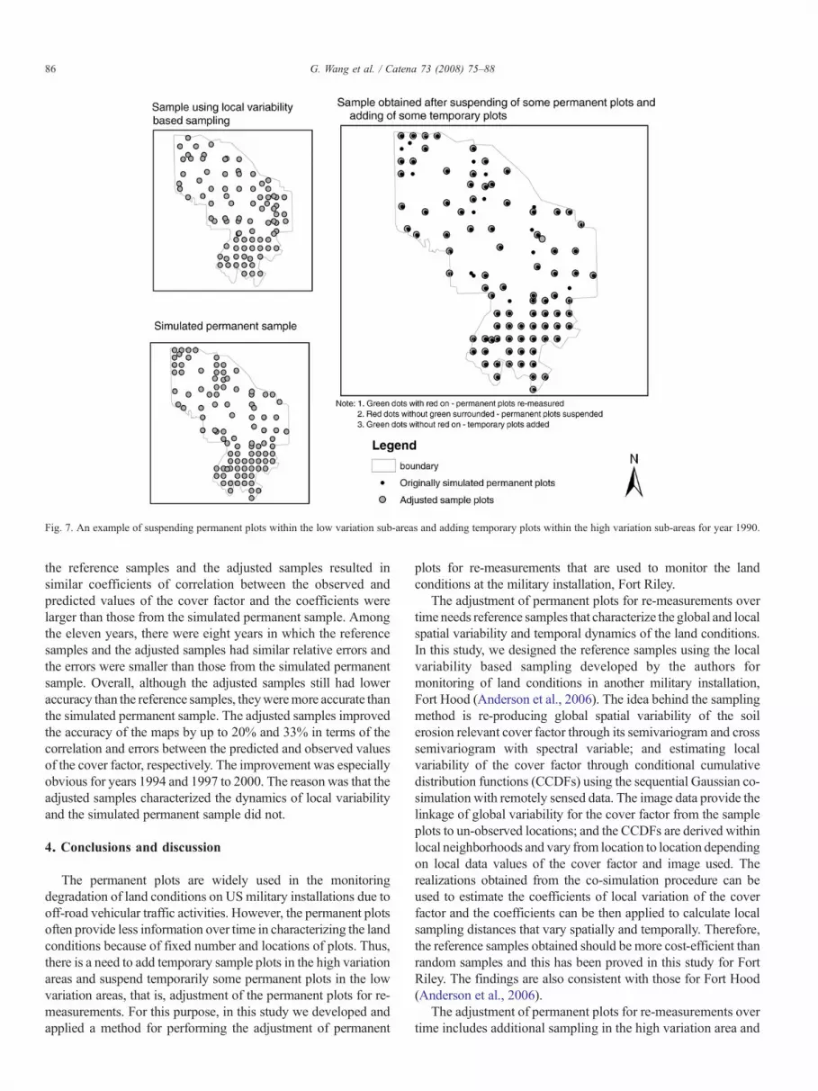
Fig. 7. An example of suspending permanent plots within the low variation sub-areas and adding temporary plots within the high variation sub-areas for year 1990.


the reference samples and the adjusted samples resulted insimilar coefficients of correlation between the observed andpredicted values of the cover factor and the coefficients werelarger than those from the simulated permanent sample. Amongthe eleven years, there were eight years in which the referencesamples and the adjusted samples had similar relative errors andthe errors were smaller than those from the simulated permanentsample. Overall, although the adjusted samples still had loweraccuracy than the reference samples, theyweremore accurate thanthe simulated permanent sample. The adjusted samples improvedthe accuracy of the maps by up to 20% and 33% in terms of thecorrelation and errors between the predicted and observed valuesof the cover factor, respectively. The improvement was especiallyobvious for years 1994 and 1997 to 2000. The reason was that theadjusted samples characterized the dynamics of local variabilityand the simulated permanent sample did not.

4. Conclusions and discussion

The permanent plots are widely used in the monitoringdegradation of land conditions on USmilitary installations due tooff-road vehicular traffic activities. However, the permanent plotsoften provide less information over time in characterizing the landconditions because of fixed number and locations of plots. Thus,there is a need to add temporary sample plots in the high variationareas and suspend temporarily some permanent plots in the lowvariation areas, that is, adjustment of the permanent plots for re-measurements. For this purpose, in this study we developed andapplied a method for performing the adjustment of permanent

plots for re-measurements that are used to monitor the landconditions at the military installation, Fort Riley.

The adjustment of permanent plots for re-measurements overtime needs reference samples that characterize the global and localspatial variability and temporal dynamics of the land conditions.In this study, we designed the reference samples using the localvariability based sampling developed by the authors formonitoring of land conditions in another military installation,Fort Hood (Anderson et al., 2006). The idea behind the samplingmethod is re-producing global spatial variability of the soilerosion relevant cover factor through its semivariogram and crosssemivariogram with spectral variable; and estimating localvariability of the cover factor through conditional cumulativedistribution functions (CCDFs) using the sequential Gaussian co-simulation with remotely sensed data. The image data provide thelinkage of global variability for the cover factor from the sampleplots to un-observed locations; and the CCDFs are derived withinlocal neighborhoods and vary from location to location dependingon local data values of the cover factor and image used. Therealizations obtained from the co-simulation procedure can beused to estimate the coefficients of local variation of the coverfactor and the coefficients can be then applied to calculate localsampling distances that vary spatially and temporally. Therefore,the reference samples obtained should be more cost-efficient thanrandom samples and this has been proved in this study for FortRiley. The findings are also consistent with those for Fort Hood(Anderson et al., 2006).

The adjustment of permanent plots for re-measurements overtime includes additional sampling in the high variation area and

Fig. 8. Comparison of the optimal samples, simulated permanent sample, and the 1 adjusted samples for mapping the cover factor in terms of (a) correlation and (b)error 2 between predicted and observed values.


suspending permanent plots in the low variation areas. In thisstudy, we used a method related to plot distances withinhomogeneous strata. That is, in an area with high variability thereference plots that are far from the permanent plots have higherprobability to become temporal plots. On the other hand, in anarea with low variability the permanent plots that are close toeach other have a higher probability to be suspended. Themethod is based on both global and local spatial variability of thevariable and takes into account the maximum representative andredundancy of plot information. The results in this study showedthat the adjusted samples were more accurate than the permanentsample to estimate the dynamics of the land conditions.

Acknowledgment

We are grateful to US Army Corps of Engineers, ConstructionEngineering Research Laboratory (USA-CERL) for providingsupport (CERLW9132T-06-2-0001) and data sets for this study.

References

Althoff, D.P., Pontius, J.S., Gipson, P., Woodford, P.B., 2005. A comprehensiveapproach to identifying monitoring priorities of small landbirds on militaryinstallations. Environmental Management 34, 887–902.

Anderson, A.B., Wang, G., Fang, S., Gertner, Z.G., Guneralp, B., 2005.Assessing and predicting changes in vegetation cover associated withmilitary land use activities. Journal of Terramechanics 42, 207–229.

Anderson, A.B., Wang, G., Gertner, G.Z., 2006. Local variability basedsampling for mapping a soil erosion cover factor by co-simulation withLandsat TM images. International Journal of Remote Sensing 27,2423–2447.

Atkinson, P.M., Webster, R., Curran, P.J., 1992. Cokriging with ground-basedradiometry. Remote Sensing of Environment 41, 45–60.

Atkinson, P.M., Webster, R., Curran, P.J., 1994. Cokriging with airborne MASSimagery. Remote Sensing of Environment 50, 335–345.

Brus, D.J., de Gruijter, J.J., 1997. Random sampling or geostatistical modeling:choosing between design-based and model-based sampling strategies forsoil (with discussion). Geoderma 80, 1–44.

Brus, D.J., Heuvelink, G.B.M., 2007. Optimization of sample patterns foruniversal kriging of environmental variables. Geoderma 138, 86–95.

Burgess, T.M., Webster, R., McBratney, A.B., 1981. Optimal interpolation andisarithmic mapping of soil properties. IV sampling strategy. Journal of SoilScience 32, 643–659.

Curran, P.J., 1988. The variogram in remote sensing: an introduction. RemoteSensing of Environment 24, 493–507.

Curran, P.J., Atkinson, P.M., 1998. Geostatistics and remote sensing. Progress inPhysical Geography 22, 61–78.

Curran, P.J., Williamson, H.D., 1986. Sample size for ground and remotelysensed data. Remote Sensing of Environment 20, 31–41.

Deutsch, C.V., Journel, A.G., 1998. Geostatistical Software Library and User'sGuide. Oxford University Press, Inc, New York, NY.

Diersing, V.E., Shaw, R.B., Tazik, D.J., 1992. US army land condition-trendanalysis (LCTA) program. Environmental Management 16, 405–414.


Dungan, J.L., 2002. Conditional simulation: An alternative to estimation forachieving mapping objective. In: Stein, A., Meer, F.V.D., Gorte, B. (Eds.),Spatial statistics for remote sensing. Kluwer Academic Publishers,Dordrecht, The Netherlands, pp. 135–152.

Goovaerts, P., 1997. Geostatistics for Natural Resources Evaluation. OxfordUniversity Press, Oxford.

Hengl, T., Rossiter, D.G., Stein, A., 2003. Soil sampling strategies for spatialprediction by correlation with auxiliary maps. Australian Journal of SoilResearch 41, 1403–1422.

Laslett, G.M., Heuvelink, G.M., Cressie, N., Urquhart, N.S., Webster, R.,McBratney, A.B., Brus, D.J., de Gruijter, J.J., 1997. Discussion of the paperby D.J. Brus and J.J. Gruijter. Geoderma 80, 45–54.

Matheron, G., 1963. Principles of geostatistics. Economic Geology 58,1246–1266.

Matheron, G., 1971. The Theory of Regionalized Variables and its Applications(Les Cahiers du center de Morphologie Mathematique de Fontainebleau 5.CMMF, Fontainebleu).

McBratney, A.B., Webster, R., 1981. The design of optimal sampling schemesfor local estimation and mapping of regionalized variables— II program andexamples. Computers & Geosciences 7, 335–365.

McBratney, A.B., Webster, R., Burgess, T.M., 1981. The design of optimalsampling schemes for local estimation and mapping of regionalizedvariables — I theory and method. Computers & Geosciences 7, 331–334.

McBratney, A.B., Webster, R., 1983a. How many observations are needed forregional estimation of soil properties. Soil Science 135, 177–183.

McBratney, A.B., Webster, R., 1983b. Optimal interpolation and isarithmicmapping of soil properties V. Co-regionalization and multiple samplingstrategy. Journal of Soil Science 34, 137–162.

Renard, K.G., Foster, G.R., Weesies, G.A., McCool, D.K., Yoder, D.C., 1997.Predicting soil erosion by water: a guide to conservation planning with therevised universal soil loss equation (RUSLE). US Department ofAgriculture, Agriculture Handbook Number 703. US Government PrintingOffice, SSOP Washington, DC.

Stein, A., Bastiaanssen, W.G.M., De Bruin, S., Cracknell, A.P., Curran, P.J.,Fabbri, A.G., Gorte, B.G.H., van Groenigen, J.W., van der Meer, F.D.,Saldan, A., 1998. Integrating spatial statistics and remote sensing.International Journal of Remote Sensing 19, 1793–1814.

Stein, A., Ettema, C., 2003. An overview of spatial sampling procedures andexperimental design of spatial studies for ecosystem comparisons.Agriculture, Ecosystems & Environment 94, 31–47.

Tazik, D.J., Warren, S.D., Diersing, V.E., Shaw, R.B., Brozka, R.J., Bagley, C.F.,Whitworth, W.R., 1992. US Army Land Condition Trend Analysis (LCTA)plot inventory field methods. USACERL, Tech. Rep. N-92/03. Dept. of theArmy, Construction Engineering Research Laboratories, Champaign, IL.

Thompson, S.K., 1992. Sampling. John Wiley & Sons, Inc, New York.Van Groenigen, J.W., Stein, A., 1998. Constrained optimization of spatial

sampling using continuous simulated annealing. Journal of EnvironmentalQuality 27, 1078–1086.

Van Groenigen, J.W., Siderius, W., Stein, A., 1999. Constrained optimization ofsoil sampling for minimization of the kriging variance. Geoderma 87,239–259.

Wang, G., Gertner, G.Z., Anderson, A.B., 2005. Sampling design anduncertainty based on spatial variability of spectral reflectance for mappingvegetation cover. International Journal of Remote Sensing 26, 3255–3274.

Wang, G., Gertner, G.Z., Anderson, A.B., 2007. Sampling and mapping a soilerosion relevant cover factor by integrating stratification, model updatingand cokriging with images. Environmental Management 39 (1), 84–97.

Wang G., Gertner G.Z., Anderson A.B., in press. Spatial variability and temporaldynamics analysis of soil erosion due tomilitary land use activities: uncertaintyand implications for land management. Land Degradation & Development.

Warrick, A.W., Myers, D.E., 1987. Optimization of sampling locations forvariogram calculations. Water Resources Research 23, 496–500.

Wischmeier, W.H., Smith, D.D., 1978. Predicting rainfall-erosion losses fromcropland east of the Rock Mountains: guide for selection of practices for soiland water conservation. USDA, Agriculture Handbook. No. 282. USGovernment Printing Office, SSOP Washington, DC, pp. 1–58.

Documents

Repeated measurements on permanent plots using local variability sampling for monitoring soil cover