SANDIA REPORTSAND2012-1750Unlimited ReleasePrinted March 2012

Report of Experiments and Evidencefor ASC L2 Milestone 4467 -Demonstration of a LegacyApplication’s Path to Exascale

Brian Barrett, Richard Barrett, James Brandt, Ron Brightwell, Matthew Curry,Nathan Fabian, Kurt Ferreira, Ann Gentile, Scott Hemmert, Suzanne Kelly, RuthKlundt, James Laros III, Vitus Leung, Michael Levenhagen, Gerald Lofstead, KenMoreland, Ron Oldfield, Kevin Pedretti, Arun Rodrigues, David Thompson, TomTucker, Lee Ward, John Van Dyke, Courtenay Vaughan, and Kyle Wheeler

Prepared bySandia National LaboratoriesAlbuquerque, New Mexico 87185 and Livermore, California 94550

Sandia National Laboratories is a multi-program laboratory managed and operated by Sandia Corporation,a wholly owned subsidiary of Lockheed Martin Corporation, for the U.S. Department of Energy’sNational Nuclear Security Administration under contract DE-AC04-94AL85000.

Approved for public release; further dissemination unlimited.

Issued by Sandia National Laboratories, operated for the United States Department of Energyby Sandia Corporation.

NOTICE: This report was prepared as an account of work sponsored by an agency of the UnitedStates Government. Neither the United States Government, nor any agency thereof, nor anyof their employees, nor any of their contractors, subcontractors, or their employees, make anywarranty, express or implied, or assume any legal liability or responsibility for the accuracy,completeness, or usefulness of any information, apparatus, product, or process disclosed, or rep-resent that its use would not infringe privately owned rights. Reference herein to any specificcommercial product, process, or service by trade name, trademark, manufacturer, or otherwise,does not necessarily constitute or imply its endorsement, recommendation, or favoring by theUnited States Government, any agency thereof, or any of their contractors or subcontractors.The views and opinions expressed herein do not necessarily state or reflect those of the UnitedStates Government, any agency thereof, or any of their contractors.

Printed in the United States of America. This report has been reproduced directly from the bestavailable copy.

Available to DOE and DOE contractors fromU.S. Department of EnergyOffice of Scientific and Technical InformationP.O. Box 62Oak Ridge, TN 37831

Telephone: (865) 576-8401Facsimile: (865) 576-5728E-Mail: reports@adonis.osti.govOnline ordering: http://www.osti.gov/bridge

Available to the public fromU.S. Department of CommerceNational Technical Information Service5285 Port Royal RdSpringfield, VA 22161

Telephone: (800) 553-6847Facsimile: (703) 605-6900E-Mail: orders@ntis.fedworld.govOnline ordering: http://www.ntis.gov/help/ordermethods.asp?loc=7-4-0#online

DE

PA

RT

MENT OF EN

ER

GY

• • UN

IT

ED

STATES OFA

M

ER

IC

A

2

SAND2012-1750Unlimited Release

Printed March 2012

Report of Experiments and Evidence for ASC L2Milestone 4467 - Demonstration of a Legacy

Application’s Path to Exascale

Brian Barrett∗, Richard Barrett∗, James Brandt,◦ Ron Brightwell∗,Matthew Curry∗, Nathan Fabian∗, Kurt Ferreira∗, Ann Gentile◦,

Scott Hemmert∗, Suzanne Kelly∗, Ruth Klundt∗, James Laros III∗,Vitus Leung∗, Michael Levenhagen∗, Gerald Lofstead∗, Kenneth Moreland∗,

Ron Oldfield∗, Kevin Pedretti∗, Arun Rodrigues∗, David Thompson,◦

Tom Tucker,� Lee Ward∗, John Van Dyke∗, Courtenay Vaughan∗, and Kyle Wheeler∗

∗◦Sandia National LaboratoriesP.O. Box ∗5800/◦9169

∗Albuquerque, NM 87185-1319/◦Livermore, CA 94550� Open Grid Computing, Inc.

Austin, TX 78759{smkelly,others}@sandia.gov

Abstract

This report documents thirteen of Sandia’s contributions to the Computational Systems andSoftware Environment (CSSE) within the Advanced Simulation and Computing (ASC) pro-gram between fiscal years 2009 and 2012. It describes their impact on ASC applications.Most contributions are implemented in lower software levels allowing for application improve-ment without source code changes. Improvements are identified in such areas as reducedrun time, characterizing power usage, and Input/Output (I/O). Other experiments are moreforward looking, demonstrating potential bottlenecks using mini-application versions of thelegacy codes and simulating their network activity on Exascale-class hardware.

3

Acknowledgments

The authors would like to thank the Red Storm, Cielo, and Cielo Del Sur operations teamsfor their support during the dedicated experiments. These systems are valuable resourcesand the teams’ prompt response ensured that we maximized our time on them.

Part of this work used resources of the Oak Ridge Leadership Computing Facility (OLCF),located in the National Center for Computational Sciences at Oak Ridge National Lab-oratory, which is supported by the Office of Science of the Department of Energy underDE-AC05-00OR22725. An award of the computer time at the OLCF was provided by theInnovative and Novel Computational Impact on Theory and Experiment (INCITE) program.

The authors would also like to thank the following teams who provided access to andinsight into the applications used in the execution of this work: CTH, Charon, SIERRA/Aria,SIERRA/Fuego, and Zoltan.

4

Contents

Nomenclature 19

1 Introduction and Executive Summary 21

2 Red Storm Catamount Enhancements to Fully Utilize Additional Coresper Node 27

2.1 Motivation for the Change . . . . . . . . . . . . . . . . . . . . . . . . . . . . . . . . . . . . . . . . . . 27

2.2 Characterizing the effect of the Enhancements . . . . . . . . . . . . . . . . . . . . . . . . . . 28

2.2.1 Details of the test . . . . . . . . . . . . . . . . . . . . . . . . . . . . . . . . . . . . . . . . . . . 28

2.2.2 Results . . . . . . . . . . . . . . . . . . . . . . . . . . . . . . . . . . . . . . . . . . . . . . . . . . . 28

2.3 Conclusion . . . . . . . . . . . . . . . . . . . . . . . . . . . . . . . . . . . . . . . . . . . . . . . . . . . . . . 30

3 Fast where: A Utility to Reduce Debugging Time on Red Storm 31

3.1 Motivation for the Implementation . . . . . . . . . . . . . . . . . . . . . . . . . . . . . . . . . . . 31

3.2 Evaluating the Impact of the New Utility . . . . . . . . . . . . . . . . . . . . . . . . . . . . . 32

3.2.1 Fast where Performance Results . . . . . . . . . . . . . . . . . . . . . . . . . . . . . . . 32

3.2.2 STAT Results . . . . . . . . . . . . . . . . . . . . . . . . . . . . . . . . . . . . . . . . . . . . . . 33

3.3 Conclusion . . . . . . . . . . . . . . . . . . . . . . . . . . . . . . . . . . . . . . . . . . . . . . . . . . . . . . 34

4 SMARTMAP Optimization to Reduce Core-to-Core Communication Over-head 35

4.1 SMARTMAP Overview . . . . . . . . . . . . . . . . . . . . . . . . . . . . . . . . . . . . . . . . . . . . 35

4.2 SMARTMAP Performance Evaluation on Red Storm . . . . . . . . . . . . . . . . . . . . 36

4.2.1 Charon Application . . . . . . . . . . . . . . . . . . . . . . . . . . . . . . . . . . . . . . . . . 36

4.2.2 Red Storm Test Platform and System Software . . . . . . . . . . . . . . . . . . . 37

5

4.2.3 Experiment Setup . . . . . . . . . . . . . . . . . . . . . . . . . . . . . . . . . . . . . . . . . . . 37

4.2.4 SMARTMAP Results . . . . . . . . . . . . . . . . . . . . . . . . . . . . . . . . . . . . . . . . 38

4.3 XPMEM Performance Evaluation on Cielo . . . . . . . . . . . . . . . . . . . . . . . . . . . . 38

4.4 Conclusion . . . . . . . . . . . . . . . . . . . . . . . . . . . . . . . . . . . . . . . . . . . . . . . . . . . . . . 40

5 Smart Allocation Algorithms 41

5.1 Background and Motivation . . . . . . . . . . . . . . . . . . . . . . . . . . . . . . . . . . . . . . . . 41

5.1.1 Approximation Algorithms . . . . . . . . . . . . . . . . . . . . . . . . . . . . . . . . . . . 42

5.1.2 Heuristic Algorithms . . . . . . . . . . . . . . . . . . . . . . . . . . . . . . . . . . . . . . . . 43

5.2 Experiments . . . . . . . . . . . . . . . . . . . . . . . . . . . . . . . . . . . . . . . . . . . . . . . . . . . . . 43

5.2.1 Details . . . . . . . . . . . . . . . . . . . . . . . . . . . . . . . . . . . . . . . . . . . . . . . . . . . . 44

5.2.2 Results . . . . . . . . . . . . . . . . . . . . . . . . . . . . . . . . . . . . . . . . . . . . . . . . . . . 44

5.2.2.1 Red Storm . . . . . . . . . . . . . . . . . . . . . . . . . . . . . . . . . . . . . . . . . 50

5.2.2.2 Cielo . . . . . . . . . . . . . . . . . . . . . . . . . . . . . . . . . . . . . . . . . . . . . . 50

5.3 Conclusions . . . . . . . . . . . . . . . . . . . . . . . . . . . . . . . . . . . . . . . . . . . . . . . . . . . . . . 51

6 Enhancements to Red Storm and Catamount to Increase Power EfficiencyDuring Application Execution 53

6.1 Introduction and Motivation . . . . . . . . . . . . . . . . . . . . . . . . . . . . . . . . . . . . . . . . 53

6.2 CPU Frequency Tuning . . . . . . . . . . . . . . . . . . . . . . . . . . . . . . . . . . . . . . . . . . . . 54

6.2.1 Results: CPU Frequency Tuning . . . . . . . . . . . . . . . . . . . . . . . . . . . . . . . 55

6.3 Network Bandwidth Tuning . . . . . . . . . . . . . . . . . . . . . . . . . . . . . . . . . . . . . . . . . 59

6.3.1 Results: Network Bandwidth Tuning . . . . . . . . . . . . . . . . . . . . . . . . . . . 60

6.4 Energy Delay Product . . . . . . . . . . . . . . . . . . . . . . . . . . . . . . . . . . . . . . . . . . . . . 62

6.5 Conclusions . . . . . . . . . . . . . . . . . . . . . . . . . . . . . . . . . . . . . . . . . . . . . . . . . . . . . . 62

7 Reducing Effective I/O Costs with Application-Level Data Services 65

7.1 Background and Motivation . . . . . . . . . . . . . . . . . . . . . . . . . . . . . . . . . . . . . . . . 65

6

7.2 Nessie . . . . . . . . . . . . . . . . . . . . . . . . . . . . . . . . . . . . . . . . . . . . . . . . . . . . . . . . . . 67

7.3 A Simple Data-Transfer Service . . . . . . . . . . . . . . . . . . . . . . . . . . . . . . . . . . . . . 69

7.3.1 Defining the Service API . . . . . . . . . . . . . . . . . . . . . . . . . . . . . . . . . . . . . 69

7.3.2 Implementing the client stubs . . . . . . . . . . . . . . . . . . . . . . . . . . . . . . . . . 70

7.3.3 Implementing the server . . . . . . . . . . . . . . . . . . . . . . . . . . . . . . . . . . . . . . 71

7.3.4 Performance of the transfer service . . . . . . . . . . . . . . . . . . . . . . . . . . . . . 72

7.4 PnetCDF staging service . . . . . . . . . . . . . . . . . . . . . . . . . . . . . . . . . . . . . . . . . . . 73

7.4.1 PnetCDF staging service performance analysis . . . . . . . . . . . . . . . . . . . 76

7.4.1.1 IOR Performance . . . . . . . . . . . . . . . . . . . . . . . . . . . . . . . . . . . 76

7.4.1.2 S3D Performance . . . . . . . . . . . . . . . . . . . . . . . . . . . . . . . . . . . . 77

7.5 Availability of Data Services Software . . . . . . . . . . . . . . . . . . . . . . . . . . . . . . . . 78

7.6 Summary and Future Work . . . . . . . . . . . . . . . . . . . . . . . . . . . . . . . . . . . . . . . . . 79

8 In situ and In transit Visualization and Analysis 81

8.1 Background . . . . . . . . . . . . . . . . . . . . . . . . . . . . . . . . . . . . . . . . . . . . . . . . . . . . . . 81

8.1.1 In situ Implementation . . . . . . . . . . . . . . . . . . . . . . . . . . . . . . . . . . . . . . . 82

8.1.2 In transit Implementation . . . . . . . . . . . . . . . . . . . . . . . . . . . . . . . . . . . . 83

8.2 Performance on Cielo . . . . . . . . . . . . . . . . . . . . . . . . . . . . . . . . . . . . . . . . . . . . . . 83

8.3 Conclusion . . . . . . . . . . . . . . . . . . . . . . . . . . . . . . . . . . . . . . . . . . . . . . . . . . . . . . 85

9 Dynamic Shared Libraries on Cielo 87

9.1 Motivation for the Implementation . . . . . . . . . . . . . . . . . . . . . . . . . . . . . . . . . . . 87

9.2 Configuration and Implementation of the Solution . . . . . . . . . . . . . . . . . . . . . . 88

9.3 Evaluating the Impact of the New Configuration . . . . . . . . . . . . . . . . . . . . . . . . 89

9.3.1 Benchmark Results . . . . . . . . . . . . . . . . . . . . . . . . . . . . . . . . . . . . . . . . . . 89

9.3.2 Application Results . . . . . . . . . . . . . . . . . . . . . . . . . . . . . . . . . . . . . . . . . 90

9.4 Conclusion . . . . . . . . . . . . . . . . . . . . . . . . . . . . . . . . . . . . . . . . . . . . . . . . . . . . . . 91

7

10 Process Replication for Reliability 93

10.1 Introduction . . . . . . . . . . . . . . . . . . . . . . . . . . . . . . . . . . . . . . . . . . . . . . . . . . . . . 93

10.2 Background . . . . . . . . . . . . . . . . . . . . . . . . . . . . . . . . . . . . . . . . . . . . . . . . . . . . . . 95

10.2.1 Disk-based Coordinated Checkpoint/Restart . . . . . . . . . . . . . . . . . . . . . 95

10.2.1.1 Current State of Practice . . . . . . . . . . . . . . . . . . . . . . . . . . . . . 95

10.2.1.2 Scaling of Coordinated Disk-based Checkpoint/Restart . . . . . 95

10.2.2 State Machine Replication . . . . . . . . . . . . . . . . . . . . . . . . . . . . . . . . . . . . 96

10.3 Replication for Message Passing HPC Applications . . . . . . . . . . . . . . . . . . . . . . 97

10.3.1 Overview . . . . . . . . . . . . . . . . . . . . . . . . . . . . . . . . . . . . . . . . . . . . . . . . . . 97

10.3.2 Costs and Benefits . . . . . . . . . . . . . . . . . . . . . . . . . . . . . . . . . . . . . . . . . . 97

10.4 Evaluating Replication in Exascale Systems . . . . . . . . . . . . . . . . . . . . . . . . . . . . 98

10.4.1 Comparison Approach . . . . . . . . . . . . . . . . . . . . . . . . . . . . . . . . . . . . . . . 98

10.4.2 Assumptions . . . . . . . . . . . . . . . . . . . . . . . . . . . . . . . . . . . . . . . . . . . . . . . 99

10.5 Model-based Analysis . . . . . . . . . . . . . . . . . . . . . . . . . . . . . . . . . . . . . . . . . . . . . . 99

10.6 Runtime Overhead of Replication . . . . . . . . . . . . . . . . . . . . . . . . . . . . . . . . . . . . 100

10.6.1 rMPI Design . . . . . . . . . . . . . . . . . . . . . . . . . . . . . . . . . . . . . . . . . . . . . . . 101

10.6.1.1 Basic Consistency Protocols . . . . . . . . . . . . . . . . . . . . . . . . . . . 101

10.6.1.2 MPI Consistency Requirements . . . . . . . . . . . . . . . . . . . . . . . . 102

10.6.1.3 Failure Detection . . . . . . . . . . . . . . . . . . . . . . . . . . . . . . . . . . . . 103

10.6.2 Evaluation . . . . . . . . . . . . . . . . . . . . . . . . . . . . . . . . . . . . . . . . . . . . . . . . . 103

10.6.2.1 Methodology . . . . . . . . . . . . . . . . . . . . . . . . . . . . . . . . . . . . . . . 103

10.6.2.2 LAMMPS . . . . . . . . . . . . . . . . . . . . . . . . . . . . . . . . . . . . . . . . . 104

10.6.2.3 SAGE . . . . . . . . . . . . . . . . . . . . . . . . . . . . . . . . . . . . . . . . . . . . . 104

10.6.2.4 CTH . . . . . . . . . . . . . . . . . . . . . . . . . . . . . . . . . . . . . . . . . . . . . . 105

10.6.2.5 HPCCG . . . . . . . . . . . . . . . . . . . . . . . . . . . . . . . . . . . . . . . . . . . 106

10.6.3 Analysis and Summary . . . . . . . . . . . . . . . . . . . . . . . . . . . . . . . . . . . . . . 106

8

10.7 Simulation-Based Analysis . . . . . . . . . . . . . . . . . . . . . . . . . . . . . . . . . . . . . . . . . . 107

10.7.1 Overview . . . . . . . . . . . . . . . . . . . . . . . . . . . . . . . . . . . . . . . . . . . . . . . . . . 107

10.7.2 Combined Hardware and Software Overheads . . . . . . . . . . . . . . . . . . . . 107

10.7.3 Scaling at Different Failure Rates . . . . . . . . . . . . . . . . . . . . . . . . . . . . . . 108

10.7.4 Scaling at Different Checkpoint I/O Rates . . . . . . . . . . . . . . . . . . . . . . . 109

10.7.5 Non-Exponential Failure Distributions . . . . . . . . . . . . . . . . . . . . . . . . . . 110

10.8 Conclusions . . . . . . . . . . . . . . . . . . . . . . . . . . . . . . . . . . . . . . . . . . . . . . . . . . . . . . 111

11 Enabling Dynamic Resource-Aware Computing 113

11.1 Introduction . . . . . . . . . . . . . . . . . . . . . . . . . . . . . . . . . . . . . . . . . . . . . . . . . . . . . 113

11.2 Infrastructure Components . . . . . . . . . . . . . . . . . . . . . . . . . . . . . . . . . . . . . . . . . 114

11.2.1 Low Impact Monitoring . . . . . . . . . . . . . . . . . . . . . . . . . . . . . . . . . . . . . . 115

11.2.1.1 Data collection . . . . . . . . . . . . . . . . . . . . . . . . . . . . . . . . . . . . . 115

11.2.1.2 Node-local Transport . . . . . . . . . . . . . . . . . . . . . . . . . . . . . . . . 116

11.2.2 Remote Transport and Storage . . . . . . . . . . . . . . . . . . . . . . . . . . . . . . . . 117

11.2.2.1 Remote transport . . . . . . . . . . . . . . . . . . . . . . . . . . . . . . . . . . . 117

11.2.2.2 Remote Storage . . . . . . . . . . . . . . . . . . . . . . . . . . . . . . . . . . . . . 118

11.2.3 Analysis . . . . . . . . . . . . . . . . . . . . . . . . . . . . . . . . . . . . . . . . . . . . . . . . . . . 118

11.2.3.1 Post-processing . . . . . . . . . . . . . . . . . . . . . . . . . . . . . . . . . . . . . 118

11.2.3.2 Run-time . . . . . . . . . . . . . . . . . . . . . . . . . . . . . . . . . . . . . . . . . . 119

11.2.3.3 Visualization . . . . . . . . . . . . . . . . . . . . . . . . . . . . . . . . . . . . . . . 119

11.2.4 Application Feedback Methods . . . . . . . . . . . . . . . . . . . . . . . . . . . . . . . . 119

11.2.4.1 Static feedback mechanisms . . . . . . . . . . . . . . . . . . . . . . . . . . . 120

11.2.4.2 Dynamic feedback mechanisms . . . . . . . . . . . . . . . . . . . . . . . . . 121

11.3 Applying the Infrastructure to Enable Resource-Aware Computing . . . . . . . . . 121

11.3.1 Applications characteristics and experimental setup . . . . . . . . . . . . . . . 121

11.3.2 Methodology used to search for appropriate indicators . . . . . . . . . . . . . 122

9

11.3.3 Aria measures of interest, feedback, and results . . . . . . . . . . . . . . . . . . . 122

11.3.3.1 Static feedback with Aria . . . . . . . . . . . . . . . . . . . . . . . . . . . . . 122

11.3.3.2 Dynamic feedback with Aria . . . . . . . . . . . . . . . . . . . . . . . . . . 123

11.3.4 Fuego measures of interest, feedback, and results . . . . . . . . . . . . . . . . . . 124

11.3.4.1 Dynamic feedback with Fuego . . . . . . . . . . . . . . . . . . . . . . . . . 125

11.4 Conclusion . . . . . . . . . . . . . . . . . . . . . . . . . . . . . . . . . . . . . . . . . . . . . . . . . . . . . . 126

12 A Scalable Virtualization Environment for Exascale 127

12.1 Introduction . . . . . . . . . . . . . . . . . . . . . . . . . . . . . . . . . . . . . . . . . . . . . . . . . . . . . 127

12.2 Application Results . . . . . . . . . . . . . . . . . . . . . . . . . . . . . . . . . . . . . . . . . . . . . . . 129

12.3 Conclusion . . . . . . . . . . . . . . . . . . . . . . . . . . . . . . . . . . . . . . . . . . . . . . . . . . . . . . 129

13 Goofy File System for High-Bandwidth Checkpoints 131

13.1 Introduction and Motivation . . . . . . . . . . . . . . . . . . . . . . . . . . . . . . . . . . . . . . . . 131

13.2 Related Work . . . . . . . . . . . . . . . . . . . . . . . . . . . . . . . . . . . . . . . . . . . . . . . . . . . . 132

13.3 The GoofyFS Storage Server and Client . . . . . . . . . . . . . . . . . . . . . . . . . . . . . . . 133

13.4 Instrumenting CTH . . . . . . . . . . . . . . . . . . . . . . . . . . . . . . . . . . . . . . . . . . . . . . . 133

13.5 Application Impact . . . . . . . . . . . . . . . . . . . . . . . . . . . . . . . . . . . . . . . . . . . . . . . . 134

13.6 Conclusion . . . . . . . . . . . . . . . . . . . . . . . . . . . . . . . . . . . . . . . . . . . . . . . . . . . . . . 135

14 Exascale Simulation - Enabling Flexible Collective Communication Offloadwith Triggered Operations 137

14.1 Introduction . . . . . . . . . . . . . . . . . . . . . . . . . . . . . . . . . . . . . . . . . . . . . . . . . . . . . 137

14.2 Triggered Operations in Portals 4 . . . . . . . . . . . . . . . . . . . . . . . . . . . . . . . . . . . . 138

14.3 Evaluation Methodology . . . . . . . . . . . . . . . . . . . . . . . . . . . . . . . . . . . . . . . . . . . 139

14.3.1 Algorithms for Allreduce . . . . . . . . . . . . . . . . . . . . . . . . . . . . . . . . . . . . . 139

14.3.1.1 Implementation with Triggered Operations . . . . . . . . . . . . . . . 139

14.3.2 Structural Simulation Toolkit v2.0 . . . . . . . . . . . . . . . . . . . . . . . . . . . . . 140

10

14.3.3 Simulated Architecture . . . . . . . . . . . . . . . . . . . . . . . . . . . . . . . . . . . . . . 140

14.3.4 Simulation Parameter Definitions . . . . . . . . . . . . . . . . . . . . . . . . . . . . . . 141

14.4 Results . . . . . . . . . . . . . . . . . . . . . . . . . . . . . . . . . . . . . . . . . . . . . . . . . . . . . . . . . 143

14.4.1 Impact of Triggered Operations . . . . . . . . . . . . . . . . . . . . . . . . . . . . . . . . 143

14.4.2 Impact of Offload on Noise Sensitivity . . . . . . . . . . . . . . . . . . . . . . . . . . 143

14.5 Conclusions . . . . . . . . . . . . . . . . . . . . . . . . . . . . . . . . . . . . . . . . . . . . . . . . . . . . . . 146

15 Application Scaling 147

15.1 Boundary Exchange with Nearest Neighbors . . . . . . . . . . . . . . . . . . . . . . . . . . . 147

15.1.1 A Case Study at High Processor Counts . . . . . . . . . . . . . . . . . . . . . . . . . 148

15.1.2 A deeper dive . . . . . . . . . . . . . . . . . . . . . . . . . . . . . . . . . . . . . . . . . . . . . . 150

15.1.3 A Hybrid MPI+OpenMP exploration . . . . . . . . . . . . . . . . . . . . . . . . . . . 153

15.2 Implicit Finite Element solver . . . . . . . . . . . . . . . . . . . . . . . . . . . . . . . . . . . . . . . 155

15.3 Conclusions and Summary . . . . . . . . . . . . . . . . . . . . . . . . . . . . . . . . . . . . . . . . . . 157

16 Conclusion 159

References 162

11

List of Figures

2.1 Node Utilization - Unused Core Percentage . . . . . . . . . . . . . . . . . . . . . . . . . . . . 29

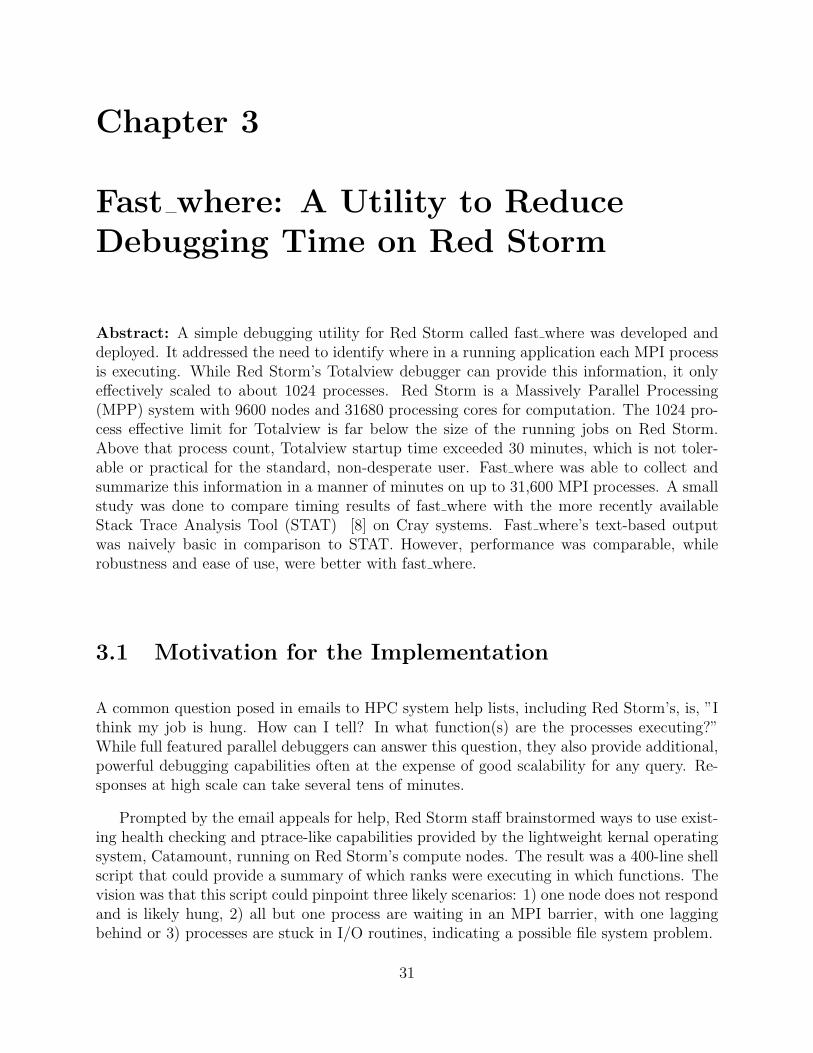
3.1 Based on the limited data points collected, fast where execution times scaledvery well with CTH. Charon results were acceptable, but difficult to interpret. 32

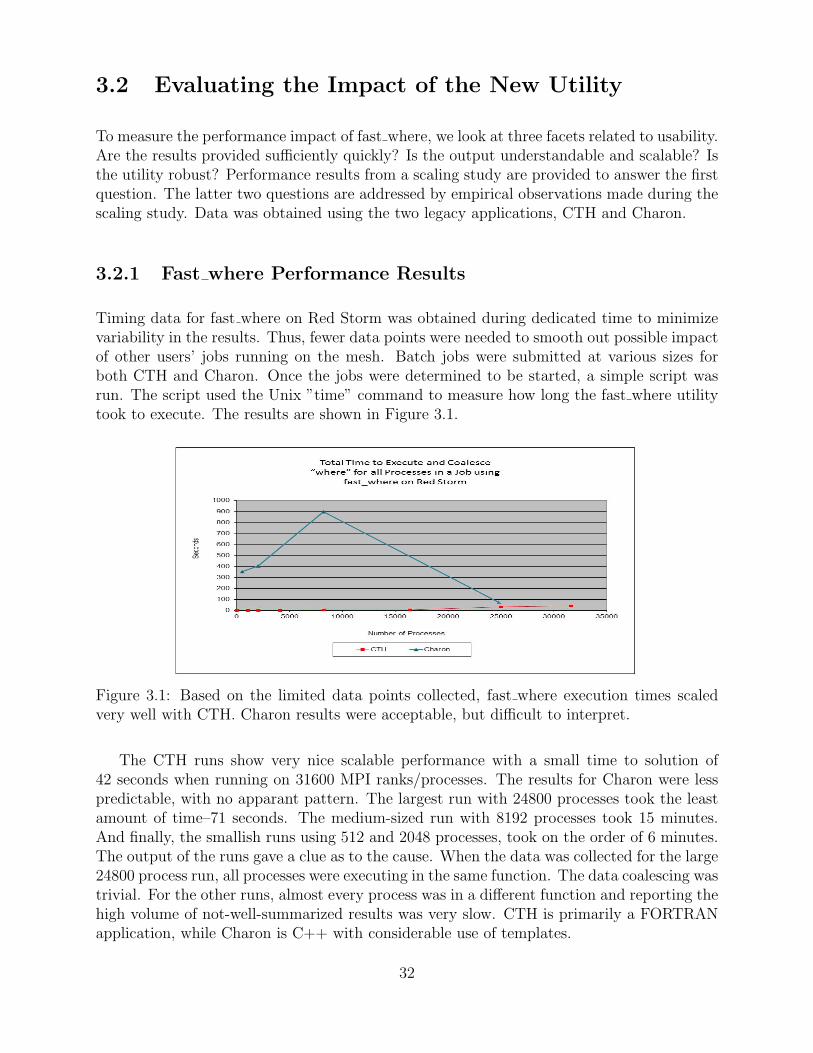
3.2 STAT timing results gave acceptable interactive response times for the datapoints obtained. However, fast where exhibited a better scaling curve. . . . . . . 34

4.1 Catamount code for converting a local address to a remote address. . . . . . . . . 36

5.1 MC and MC1x1. . . . . . . . . . . . . . . . . . . . . . . . . . . . . . . . . . . . . . . . . . . . . . . . . . . 42

5.2 Gen-Alg, Hilbert curve, and “snake” curve. . . . . . . . . . . . . . . . . . . . . . . . . . . . . 42

5.3 The run and completion times for the runs of the job stream derived fromwindow one on Red Storm. . . . . . . . . . . . . . . . . . . . . . . . . . . . . . . . . . . . . . . . . . 45

5.4 The run and completion times for the runs of the job stream derived fromwindow two on Red Storm. . . . . . . . . . . . . . . . . . . . . . . . . . . . . . . . . . . . . . . . . . 46

5.5 The run and completion times for the run of the job stream derived fromwindow three on Red Storm. . . . . . . . . . . . . . . . . . . . . . . . . . . . . . . . . . . . . . . . . 47

5.6 The run and completion times for the runs of the job stream derived fromwindow three on Cielo. . . . . . . . . . . . . . . . . . . . . . . . . . . . . . . . . . . . . . . . . . . . . . 48

5.7 The run and completion times for the runs of the job stream derived fromwindow two on Cielo. . . . . . . . . . . . . . . . . . . . . . . . . . . . . . . . . . . . . . . . . . . . . . . 49

6.1 Application Energy Signatures of AMG2006 and LAMMPS run at P-states 1-4 56

6.2 Normalized Energy, Run-time and (E ∗ Tw) where (w) = 1, 2, or3 . . . . . . . . . . 62

7.1 A data service uses additional compute resources to perform operations onbehalf of an HPC application. . . . . . . . . . . . . . . . . . . . . . . . . . . . . . . . . . . . . . . . 67

12

7.2 Network protocol for a Nessie storage server executing a write request. Theinitial request tells the server the operation and the location of the clientbuffers. The server fetches the data through RDMA get commands until ithas satisfied the request. After completing the data transfers, the server sendsa small “result” object back to the client indicating success or failure. . . . . . . 68

7.3 Portion of the XDR file used for a data-transfer service. . . . . . . . . . . . . . . . . . . 70

7.4 Client stub for the xfer write rdma method of the transfer service. . . . . . . . . 71

7.5 Server stub for the xfer write rdma method of the transfer service. . . . . . . . . 72

7.6 Comparison of xfer-write-encode and xfer-write-rdma on the Cray XE6platorm using the Gemini network transport. . . . . . . . . . . . . . . . . . . . . . . . . . . 73

7.7 System Architecture . . . . . . . . . . . . . . . . . . . . . . . . . . . . . . . . . . . . . . . . . . . . . . . 74

7.8 Measured throughput of the IOR benchmark code on Thunderbird . . . . . . . . . 77

7.9 Writing performance on JaguarPF one staging node (12 processes) . . . . . . . . . 78

8.1 The ParaView Coprocessing Library generalizes to many possible simulations,by means of adaptors. These are small pieces of code that translate datastructures in the simulation’s memory into data structures the library canprocess natively. In many cases, this can be handled via a shallow copy ofarray pointers, but in cases where that is not possible, it must perform a deepcopy of the data. . . . . . . . . . . . . . . . . . . . . . . . . . . . . . . . . . . . . . . . . . . . . . . . . . . 82

8.2 Block processing rate of simulation and visualization at growing scales onCielo. Note that 256 and 16384 core counts are repeated twice. This isan overlap where the block count was increased in order to continue scalingeffectively. Gaps are locations where memory errors are preventing execution. 83

8.3 Generating a contour on an AMR mesh requires special processing at theboundary between two different resolutions. Degenerate triangles must becreated to close the seams between the otherwise irregularly shaped boundary,as shown in this figure. . . . . . . . . . . . . . . . . . . . . . . . . . . . . . . . . . . . . . . . . . . . . . 84

8.4 Block processing rate of AMR contouring at growing scales on Cielo. The twodifferent lines represent different AMR sizes. Large depth means more blocksare in the simulation. . . . . . . . . . . . . . . . . . . . . . . . . . . . . . . . . . . . . . . . . . . . . . . 85

8.5 Running on Redsky, the block processing rate of AMR pipeline at growingscales compared with the simulation processing rate. . . . . . . . . . . . . . . . . . . . . 86

9.1 Fifty DVS servers were added to serve both system and user dynamic sharedlibraries to compute nodes. . . . . . . . . . . . . . . . . . . . . . . . . . . . . . . . . . . . . . . . . . 89

13

9.2 Pynamic timing results gave acceptable results only with the special purposefile system. . . . . . . . . . . . . . . . . . . . . . . . . . . . . . . . . . . . . . . . . . . . . . . . . . . . . . . 90

9.3 Based on a small number of data points, dynamic shared libraries negativelyimpact application run time. . . . . . . . . . . . . . . . . . . . . . . . . . . . . . . . . . . . . . . . . 91

10.1 Modeled application efficiency with and without state machine replication fora 168-hour application, 5-year per-socket MTBF, and 15 minute checkpointtimes. Shaded region corresponds to possible socket counts for an exascaleclass machine [17]. . . . . . . . . . . . . . . . . . . . . . . . . . . . . . . . . . . . . . . . . . . . . . . . 100

10.2 Basic replicated communication strategies for two different rMPI message con-sistency protocols. Additional protocol exchanges are needed in special casessuch as MPI ANY SOURCE. . . . . . . . . . . . . . . . . . . . . . . . . . . . . . . . . . . . . . . . . . . . 101

10.3 LAMMPS rMPI performance comparison. For both mirror and parallel base-line performance overhead is equivalent. For this application the performanceof forward, reverse, and shuffle fully redundant is equivalent. . . . . . . . . . . . . . . 104

10.4 SAGE rMPI performance comparison. For both mirror and parallel baselineperformance overhead is equivalent. For this application the performance offorward, reverse, and shuffle fully redundant is equivalent. . . . . . . . . . . . . . . . . 105

10.5 CTH rMPI performance comparison. For both mirror and parallel baselineperformance overhead is equivalent. For this application the performance offorward, reverse, and shuffle fully redundant is equivalent. . . . . . . . . . . . . . . . . 105

10.6 HPCCG rMPI performance comparison. Varying performance for native andbaseline between mirror and parallel protocols is due to different node alloca-tions. . . . . . . . . . . . . . . . . . . . . . . . . . . . . . . . . . . . . . . . . . . . . . . . . . . . . . . . . . . . 106

10.7 Simulated application efficiency with and without replication including rMPIrun time overheads. Shaded region corresponds to possible socket counts foran exascale class machine [17]. . . . . . . . . . . . . . . . . . . . . . . . . . . . . . . . . . . . . . . 108

10.8 Simulated replication break-even point assuming a constant checkpoint time(δ) of 15 minutes. Shaded region corresponds to possible socket counts andMTBFs for an exascale class machine [17]. Areas of the shaded region wherereplication uses less resources are above the curve. Areas below the curve arewhere traditional checkpoint/restart uses lower resources. . . . . . . . . . . . . . . . . 109

14

10.9 “Break even” points for replication for various checkpoint bandwidth rates.The shaded region corresponds to possible socket counts and socket MTBFsfor exascale class machines [17]. State machine replication is a viable ap-proach for most checkpoint bandwidths, but with a checkpoint bandwidthgreater than 30TB/sec, replication is inappropriate for the majority of theexascale design space. Areas of the shaded region where replication uses lessresources are above the curve. Areas below the curve are where traditionalcheckpoint/restart uses lower resources. . . . . . . . . . . . . . . . . . . . . . . . . . . . . . . 110

10.10Comparison of simulated application efficiency with and without replication,including rMPI run time overheads, using a Weibull and Exponential faultdistribution. In both these figures we assume a checkpoint bandwidth of1TB/sec. The shape parameter (β) 0.156 and MTBF corresponds to the RPIBlueGene system [63]. Shaded region corresponds to possible socket countsfor an exascale class machine [17]. . . . . . . . . . . . . . . . . . . . . . . . . . . . . . . . . . . . 111

11.1 Integration of capabilities for Low Impact Monitoring, Transport and Storage,Analysis, and Feedback to enable Resource-Aware Computing . . . . . . . . . . . . . 115

11.2 Monitoring infrastructure overhead with respect to CPU and memory foot-print. Impact on CPU resources with respect to the total available on this 16core per node system are shown in the upper left while that for running on adedicated core (using corespec (Section 11.3.3.1) is shown in the upper right.Memory footprint in MiB is shown in the lower left while that as a fraction ofthe 32GB available is shown in the lower right. Note that these figures showoverhead on a per component basis and that the total is shown in parenthesesin the X-axis label. . . . . . . . . . . . . . . . . . . . . . . . . . . . . . . . . . . . . . . . . . . . . . . . 116

11.3 Screenshot of visualization tool showing system processes across the 576 nodesof Cielo Del Sur (Cray XE6) with no application running. Each horizontalrow represents data values for each of 16 cores on each of 6 nodes (separatedby fine bands). Note that white stripes represent nodes for which data wasnot being collected (e.g. service nodes or out of service). The color schemehighlights system process utilization with red being zero ticks and blue beingthree. . . . . . . . . . . . . . . . . . . . . . . . . . . . . . . . . . . . . . . . . . . . . . . . . . . . . . . . . . . . 120

11.4 Partition Distributions for selected timesteps for an 8310 processor run of anAria example on CDS. Processors exhibiting larger ratio of idle cycles to totalcycles utilized since the last partitioning are assigned a larger partition size.Uniform partition sizes (left) results in tighter distributions than those withoutfeedback. In the feedback case, when too broad a partitioning occurs early(right, green), the partitioning feedback criteria will adjust the distribution(right, blue and magenta). . . . . . . . . . . . . . . . . . . . . . . . . . . . . . . . . . . . . . . . . . . 124

15

11.5 Particle Distributions in the Partitioning Evolution in a Fuego problem (a)after a rebalance (top) (b) after a few timesteps before the next rebalance(middle) (c) after the next rebalance (bottom) (d) without feedback (leftcolumn) (e) with feedback (right column). Rebalancing in general seeks toprovide an even distribution but is not in practice completely uniform (topand bottom). As the problem evolves and particles move the distributionwidens triggering the need for rebalancing (middle). . . . . . . . . . . . . . . . . . . . . . 125

11.6 Simple demonstration of resource evaluation and feedback shows improvementin computational cycles across all processors involved. Greater fractional uti-lization of CPU cycles is achieved with feedback than without (green) Note:Y axis is the fractional utilization of available CPU cycles and goes from 0.9to 1.0. X axis is a core unique identifier. . . . . . . . . . . . . . . . . . . . . . . . . . . . . . . 126

12.1 Block diagram of Kitten LWK running a user application natively alongsidea user application running inside a virtualized environment. . . . . . . . . . . . . . . . 128

12.2 Comparison of CTH (top) and Sage (bottom) applications running natively vs.in a virtualized environment with shadow (software) paging memory manage-ment vs. in a virtualized environment with nested (hardware) paging memorymanagement. The results show that the virtualized environment introducesless than 5% overhead in all cases. . . . . . . . . . . . . . . . . . . . . . . . . . . . . . . . . . . . 130

13.1 Average checkpoint time for GoofyFS versus PanFS. . . . . . . . . . . . . . . . . . . . . 134

14.1 Function definitions for Portals pseudo-code . . . . . . . . . . . . . . . . . . . . . . . . . . . 140

14.2 Pseudo-code for allreduce algorithms based on Portals 4 triggered operations. 141

14.3 High level NIC architecture annotated with key portals simulation timings.Timings are shown as a percentage of back-to-back latency along with absolutevalues for 1000 ns latency. . . . . . . . . . . . . . . . . . . . . . . . . . . . . . . . . . . . . . . . . . . 142

14.4 Allreduce time for 1000 ns message latency. Simulation results show thattriggered operations provide approximately 30% better allreduce latency overhost based implementations. . . . . . . . . . . . . . . . . . . . . . . . . . . . . . . . . . . . . . . . . 144

14.5 Allreduce time for 1500 ns message latency. Simulation results show that trig-gered opertions provide greater than 40% better allreduce latency comparedto host based implementations. . . . . . . . . . . . . . . . . . . . . . . . . . . . . . . . . . . . . . . 144

14.6 Allreduce performance under varying noise signatures. Simulation resultsshow that offloaded triggered operations are much less sensitive to varioustypes of noise than comparable host based algorithms. . . . . . . . . . . . . . . . . . . . 145

16

15.1 CTH: Multilayered thin-walled structure torn apart by an explosive blast . . . 148

15.2 CTH performance by time steps (cycles) at 32k processor cores . . . . . . . . . . . . 149

15.3 CTH and miniGhost ommunication patterns. . . . . . . . . . . . . . . . . . . . . . . . . . . 150

15.4 CTH and miniGhost space-time runtime profiles . . . . . . . . . . . . . . . . . . . . . . . . 151

15.5 CTH and miniGhost performance comparison on a Cray XT5. . . . . . . . . . . . . 152

15.6 miniGhost weak scaling on Cielo . . . . . . . . . . . . . . . . . . . . . . . . . . . . . . . . . . . . . 152

15.7 The XE6 compute node architecture. Images courtesy of Cray, Inc. . . . . . . . . 154

15.8 miniGhost configured for MPI and OpenMP. . . . . . . . . . . . . . . . . . . . . . . . . . . . 154

15.9 Charon run time profiles, illustrated using 64 processor cores . . . . . . . . . . . . . . 155

15.10Charon on Dawn . . . . . . . . . . . . . . . . . . . . . . . . . . . . . . . . . . . . . . . . . . . . . . . . . 156

17

List of Tables

2.1 Summary of Node Utilization Test Details . . . . . . . . . . . . . . . . . . . . . . . . . . . . . 30

4.1 SMARTMAP/Catamount on Red Storm, Charon Solution Time . . . . . . . . . . . 38

4.2 SMARTMAP/Catamount on Red Storm, Charon Overall Elapsed Time . . . . . 38

4.3 XPMEM/Linux on Cielo, Charon Solution Time . . . . . . . . . . . . . . . . . . . . . . . . 39

4.4 XPMEM/Linux on Cielo, Charon Overall Elapsed Time . . . . . . . . . . . . . . . . . 39

6.1 Experiment 1: CPU Frequency Scaling: Run-time and CPU Energy %Differ-ence vs. Baseline . . . . . . . . . . . . . . . . . . . . . . . . . . . . . . . . . . . . . . . . . . . . . . . . . 58

6.2 Experiment 2: Network Bandwidth: Run-time and Total Energy %Differencevs. Baseline . . . . . . . . . . . . . . . . . . . . . . . . . . . . . . . . . . . . . . . . . . . . . . . . . . . . . . 58

14.1 Summary of Simulation Parameters . . . . . . . . . . . . . . . . . . . . . . . . . . . . . . . . . . 143

16.1 Summary of Contributions by Performance Improvement Area . . . . . . . . . . . . 161

18

Nomenclature

ASC Advanced Simulation and Computing

BSP Bulk Synchronous Processing

Core A computational unit that reads and executes program instructions.

CSSE Computational Systems and Software Engineering

FC Fiberchannel

HPC High Performance Computing

HSN High Speed Network

jMTTI Job Mean Time To Interrupt - any hardware or system software error or failurethat results in a job failure.

MPP Massively Parallel Processing

NFS Network File system

NIC Network Interface Chip

Node A network endpoint containing one or more cores that share a common memory. ForHPC, batch schedulers often reserve nodes as a minimum unit of allocation.

PTAS Polynomial-time approximation scheme

RDMA Remote Direct Memory Access

sMTTI System Mean Time To Interrupt - any hardware or system software error or failure,or cumulative errors or failures over time, resulting in more than 1% of the system beingunavailable at any given time.

19

20

Chapter 1

Introduction and Executive Summary

As part of its mission, the CSSE sub-program within ASC is responsible for deploying keysoftware components. These include system software and tools, input/output, storage sys-tems, networking, and post-processing tools. Some work is on-going in nature, some activitiesaddress short term requirements, and others address the need to invest in technology de-velopment for anticipated future mission requirements. This milestone report covers thework done within Sandia’s CSSE program to support the ASC applications as computertechnology evolves.

We begin with the milestone description:

Cielo is expected to be the last capability system on which existing ASCcodes can run without significant modifications. This assertion will be tested todetermine where the breaking point is for an existing highly scalable application.The goal is to stretch the performance boundaries of the application by applyingrecent CSSE RD in areas such as resilience, power, I/O, visualization services,SMARTMAP, lightweight LWKs, virtualization, simulation, and feedback loops.Dedicated system time reservations and/or CCC allocations will be used to quan-tify the impact of system-level changes to extend the life and performance of theASC code base. Finally, a simulation of anticipated exascale-class hardware willbe performed using SST to supplement the calculations.

The milestone team collected Sandia’s recent CSSE project activities that strive to im-prove application performance without (or with minimal) source code changes to the ap-plication. Work is from FY09, when the milestone was originally developed, through thesecond quarter of FY12. Thirteen activities are highlighted herein. They are:

• Catamount enhancements to fully utilize cores per node

• Utility to reduce debugging time on Red Storm

• Optimizations to reduce core-to-core communication overhead

• Improved node allocation algorithms

• Enhancements to increase power efficiency during application execution on Red Storm

21

• Application-level data services to reduce effective I/O costs

• In situ and in transit visualization and analysis

• Dynamic shared libraries on Cielo

• Process replication for reliability

• Enabling dynamic resource-aware computing

• Scalable virtualization environment

• File system for high bandwidth checkpoints

• Exascale simulation to enable collective communication offload

For each area, we identified and measured the performance impact using whichever unit ofmeasure was most applicable. Performance was not constrained to the most narrow definitionof “runs faster”. In addition to improved/decreased runtime, some technologies offers betterthroughput of jobs, some improve user productivity, some offer efficiency improvments, othersincrease job resiliency, etc. Some of the work targeted future technologies and provided designdata with an estimate for the expected improvement.

The milestone text references “an existing highly scalable application”. We gathereddata primarily using the CTH [44] and/or Charon [83] ASC applications. In a few cases,neither application exhibited the feature or issue being addressed by the milestone area. Inthat case, one or more different applications were used. Over time, we decided it was notnecessary to down-select to an existing application. Each application provided interestingdata that added value to the milestone results. All results are provided.

To address the “breaking point” portion of the milestone, we analyzed both CTH andCharon to determine where the scalability fell off, even with the available CSSE enhance-ments. We also estimated, using CTH’s mini-app, the cross over point when the currentCTH mpi-everywhere programming model was surpassed by on-node OpenMP and inter-node MPI. This analysis can be found in chapter 15.

Chapters 2 through 14 each address one of the thirteen development areas listed above.The chapters are sequenced primarily by platform, with the oldest targeted platform first.This translates to Red Storm, Cielo, and future platforms. Although the system is nowretired, the Red Storm work offered interesting techniques and lessons learned as we continueon the path to exascale. A number of these early chapters compare the results with theequivalent Cielo tool giving us insight into the value of lightweight kernels. Each chapterbegins with an abstract that presents the problem, describes the solution approach, andgives a very brief summary of the results of the work. The reader is encouraged to reviewjust the chapter abstracts if only the highlights are desired. However, it is best to read thefull content of each chapter in order to understand the environment under which the datawas collected.

22

The remainder of this chapter gives an executive summary. Instead of the historical orderused for sequencing the chapters, we summarize the work by the areas of improvement. Thesame caution about the risk of taking the results out of context from the test setup applieshere as well.

Reduced runtime We document six different R&D contributions that can reduce theruntime for applications.

The SMARTMAP optimization was installed into the Red Storm’s lightweight kerneloperating system, Catamount. The production MPI library was then modified to take ad-vantage of this very efficient on-node shared memory capability to reduce completion timesfor collective communication operations. Results indicate that SMARTMAP provides a 4.5%improvement in performance when running Charon on 2,048 quad-core compute nodes (8,192cores) of Red Storm. See chapter 4 for more information.

Smart algorithms for allocating available nodes to jobs can have a significant effect ontheir runtime. For networks configured as a mesh or torus, a cube-like allocation of nodesreduces distance between communicating pairs and minimizes the impact of traffic fromother jobs on the system. The initial Sandia-developed algorithm has been implemented inthe Cray scheduler by Cray. The experiment documented herein shows that the magnitudeof the improvement increased by tenfold when the average job running time of the sampleincreased by less than twenty percent. See chapter 5 for more information.

The Trilinos I/O Support (Trios) capability has been released as part of the Trilinosproject. It includes the infrastucture for application-level data services. When combinedwith an I/O service, such as PnetCDF and netCDF, it can provide an effective I/O rate thatis 10X higher for a single shared file. The application is free to continue its computationwhile the staged data is written to disk. See chapter 7 for more information.

The ability to adapt computation based on dynamically available resource utilizationinformation has been identified as an enabler for applications running at exascale. Wedemonstrate such a mechanism on Cielo, proving the feasibility of dynamic resource-awarecomputing. The capability is very lightweight consuming less than a hundredth of a percentof the computing resource. It has a scalable implementation and was demonstrated on 10,000cores. It provides both static and dynamic feedback mechanisms for the application or alibrary. See chapter 11 for more information.

We introduce a new file system concept and project, currently called GoofyFS. It is tar-geted for exascale-class systems. Quality of service is maximized by supporting multiple datastorage devices and by allowing for local decision making. The first large-scale experimenton Cielo used off-node memory to write checkpoint files, which resulted in a 10-60x speedupin effective I/O rates. See chapter 13 for more information.

Reduced runtime was a goal of an exascale hardware design as well. The design offloadscollective communication processing to a potential new NIC architecture. Under simulation,when coupled with the new version 4 of the Portals networking protocol, it is possible toachieve lower latency and higher tolerance to system noise. The simulations, run up to

23

32,768 nodes, show a 40% reduction in latency over host-based collectives processing. Seechapter 14 for more information.

Improved Job Throughput: Three chapters report on contributions that can increasethe job throughput on a system. The jobs do not necessarily run faster, but system utilizationis improved.

The job management software on Red Storm was modified to allow the user to specifyresources based on units more intuitive to their problem setup. Instead of nodes, the userspecifies the number of needed processing elements (aka MPI ranks) and optionally, theamount of memory needed per procesing element. This more natural specification was mo-tivated initially by the fact that nodes on Red Storm are heterogeneous. Nodes could haveeither two or four processing elements and the amount of memory per processing elementvaried as well. Without the change, an allocation based on nodes had to assume only twoprocessing elements and the smallest amount of memory per node. Allocation based on themost conservative node architecture wastes processors and memory. An experiment was runthat showed the modification to the allocation specification improved overall job throughputby 10% as well as enhanced the user interface. See chapter 2 for additional information.

Traditionally, the computation and visualization portions of a problem analysis have beenperformed separately. Data files are written to disk during the computation phase. The filesare then read during a separate visualization phase. Computational capabilities continue tooutpace I/O and disk technological advances. To address this ever widening gap, in situ andin transit visualization techniques are being developed to reduce the amount of required I/Oto disk. Modifying the standard HPC workflow can shrink the time from initial meshing tofinal results. Chapter 8 describes the progress to date, which will be further documented inan FY13 L2 milestone.

Although counter-intuitive, process replication can provide job throughput improvementsdepending on job size and job mean time to interrupt. We describe a prototype implemen-tation to understand runtime overhead of replication. Modeling, empirical analysis andsimulation are used to find the cross over curves where replication can be more efficientthan traditional file-based checkpoint/restart solutions for resiliency. This data is extremelyuseful for exascale regimes. See chapter 10 for more information.

Increased User Productivity: Four of the R&D contributions improve user produc-tivity. Depending on the specific area, these contributions may cause an increase in jobruntime. For these situations, the increase in runtime is quantified, as user productivity canbe a subjective measure.

A debugging utility called fast where was provided on Red Storm to help understandwhat might be going on when a job appears hung. The TotalView debugger can perform thesame function. However on Red Storm it was taking 30 minutes for TotalView to attach to1024 processes. The fast where utility was able to collect the required information in a fewminutes on 31,600 cores. See chapter 3 for more information.

The in situ and in transit visualization capabilities described above are also anticipated

24

to improve user productivity because of the compressed workflow.

Statically linked application binaries have traditionally been mandated for the jobs run-ning at the largest scales. However, dynamically linked binaries introduce productivityenhancements for application developers. It is not necessary to relink the application everytime a library is changed. Also, some applications are so large they are forced to staticallyrelink for each combination of modules needed for the problem being analyzed. At a mini-mum, this is a difficult bookkeeping task. The Cielo team implemented a hierarchical cachefor active shared libraries and ran an experiment to assess its efficiency. Based on bench-marks, the setup appeared optimal. However, the dynamically linked version of Charon ran34% longer than the statically linked version. The traditional wisdom of statically linkedbinaries prevails, unless circumstances dictate the use of a dynamically linked binary. Seechapter 9 for more information.

Application developers are often concerned about the portability of their application.Virtualization can provide multiple operating systems on a single hardware platform. Thisallows the application to operate in an environment most suitable to its needs. The Kittenoperating system, working in concert with the Palacios virtual machine monitor, can providea highly scalable lightweight kernel environment and also support applications requiring aricher set of functionalty. Experiments shows a 5% increase in runtime when running ina virtual machine, rather than directly on the hardware itself. See chapter 12 for moreinformation.

Reduced Power Consumption: In 2008, the Red Storm lightweight kernel operatingsystem, Catamount, was modified to automatically transition to lower power states whenidle. As part of this work, we developed scalable measuring techniques to quantify thepower savings of the change. This somewhat ancillary activity created a capability that canidentify additional opportunities for reduced power consumption. In this report we discussresearch that identifies the impact of reduced power states on a per job basis. In a seriesof experiments we characterize the effect of CPU frequency and network bandwidth tuningon power usage and demonstrate energy savings of up to 39% with little to no impact onruntime performance.

Data for Co-Design: Most of the activities discussed so far inform our exascale co-design efforts. Of particular note are 1) power efficiency, 2) new visualization workflowtechniques, 3) process replication for reliability, and 4) virtualization.

Chapter 15 is specifically targeted at scalability. We studied the CTH and Charon ap-plications to identify bottlenecks that we expect to be issues as machines and applicationsapproach exascale. There was no single breaking point found. In fact, several different oneswere found for CTH and Charon. System software scalability issues remain, even with theenhancements documented herein. An analysis was performed estimating the breaking pointfor the MPI-everywhere programming model within CTH. Algorithmic improvements wereidentified to improve Charon scalability.

Given this introduction and summary of the work, we hope you are inspired to read more

25

of the document in the areas that interest you.

26

Chapter 2

Red Storm Catamount Enhancementsto Fully Utilize Additional Cores perNode

Abstract: Enhancements to the job submission interface are described here which enablemore efficient core utilization by accepting requests for compute resources using parametersthat match the requirements of the application. This spares the user the task of remappingthose requirements to the peculiarities of the hardware configuration, which may be compli-cated by heterogeneity and may be evolving. Experiments are described that demonstrateda 10% improvement in core utilization using sampled actual job mixes from Red Storm.

2.1 Motivation for the Change

The Red Storm computer and Catamount, its lightweight compute node operating system,evolved over the years through multiple hardware upgrades. Throughout most of Red Storm’slifetime, as a result of partial system hardware upgrades, its hardware has been heterogeneouswith a varying number of compute cores per node and a varying amount of memory per node.The software enhancements described and evaluated here were developed and installed toallow seamless full utilization of the processors in such a heterogeneous environment.

Before these changes, the user requested some number of nodes from Moab, the batch jobscheduler, but had to specify the number of cores (MPI ranks) per node to use to Yod, theCatamount program that loads and oversees a particular parallel job. There was a quad-corebatch queue available, restricting jobs to only run on quad-core nodes. The standard queueincluded all the nodes. Thus unless one submitted their job to the quad-core queue, theycould only assume there were 2 cores per node available. This conservative assumption couldmean that not all cores were fully utilized on each allocated node. The changes describedhere allow the user to request the more natural number, the number of ranks needed andoptionally the amount of memory per rank that the job requires. It is then up to thesystem to load the job on dual-core nodes, quad-core nodes or a mixture to fully utilize theprocessors. It’s easy and in the language of the application to specify to Moab the number ofranks needed and optionally the memory per rank needed. It’s more cumbersome to specify

27

to Yod how many cores per node are consistent with the memory requirements per rank andwith the queue choice and then calculate how many nodes need to be requested from Moab.The enhancement described here required change to both Moab and to Yod.

2.2 Characterizing the effect of the Enhancements

To measure the performance impact of these changes, three run streams were created. Thecore utilizations were compared by running each of these streams twice on Red Storm, oncewith the changes ( “new way”) and once emulating the environment without (“old way”).To do this, three two-week windows of actual Red Storm usage were selected from beforethese changes were introduced. For each of those windows, the number of nodes used, theelapsed time of job execution (truncated to minutes) and a flag to indicate whether the jobran in the quad-core batch queue was collected from the Accounting Database. Very smalljobs, less than 9 nodes or less than 20 minutes, were excluded.

2.2.1 Details of the test

The creation, submitting and running in the two modes differed in three ways. (1) SeparateBourne shell scripts were used for the each mode to read the job list file and submit the jobsto Moab. Each submission requested a Yod enforced time limit of the scaled run time. SinceMoab now needs requested cores instead of requested node, for the new way, the number ofrequested cores was two or four times the number of nodes depending on the quad-queue flag.For the emulation mode, the number of requested cores from Moab was always artificiallyset to twice the number of nodes. If the quad-queue flag was set, that information waspassed on to Moab and used in creating the Yod command line. (2) The currently installedMoab program was used for all runs, but for emulation mode, the node description in theMoab configuration file was changed by specifying that all nodes had two cores per node.Fortunately the current Moab has a separate specification tag of node type. Thus specify“quad” could be used to force a job to quad-core nodes. (3) For emulation mode only, amodified Yod was then used that tweaked the loading information so that non-quad-queuejobs were forced to use 2 cores per node no matter which node they ran on and to enablequad-queue jobs to utilize 4 cores. The shock physics code, CTH, was used for all of thejobs. The submission scripts configured the run to use the appropriate number of ranks.

2.2.2 Results

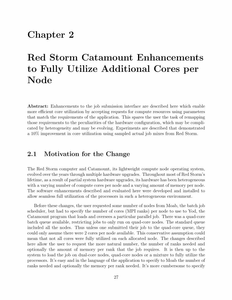
The results for core utilization are shown in Figure 2.1, which plot the percent of unusedcores throughout the runs of the job streams derived from window one. Visually it appearsthat the average number of unused cores is less the new way, i.e. the core utilization isbetter. To reduce the end effects as the queue emptied, the comparisons were done using the

28

average core utilization computed over the period up until the work done in the job streamwas 90 percent completed. In the figures the three squares in the upper right mark the 85,90 and 95 percent core-hours point. The results would not be particularly different if 85percent or 95 percent had been chosen.

Figure 2.1: Node Utilization - Unused Core Percentage

29

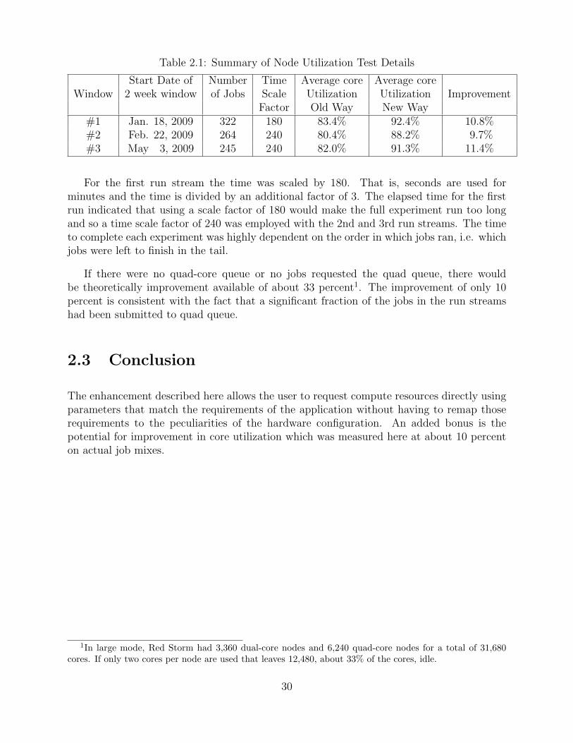
Table 2.1: Summary of Node Utilization Test Details

Start Date of Number Time Average core Average coreWindow 2 week window of Jobs Scale Utilization Utilization Improvement

Factor Old Way New Way#1 Jan. 18, 2009 322 180 83.4% 92.4% 10.8%#2 Feb. 22, 2009 264 240 80.4% 88.2% 9.7%#3 May 3, 2009 245 240 82.0% 91.3% 11.4%

For the first run stream the time was scaled by 180. That is, seconds are used forminutes and the time is divided by an additional factor of 3. The elapsed time for the firstrun indicated that using a scale factor of 180 would make the full experiment run too longand so a time scale factor of 240 was employed with the 2nd and 3rd run streams. The timeto complete each experiment was highly dependent on the order in which jobs ran, i.e. whichjobs were left to finish in the tail.

If there were no quad-core queue or no jobs requested the quad queue, there wouldbe theoretically improvement available of about 33 percent1. The improvement of only 10percent is consistent with the fact that a significant fraction of the jobs in the run streamshad been submitted to quad queue.

2.3 Conclusion

The enhancement described here allows the user to request compute resources directly usingparameters that match the requirements of the application without having to remap thoserequirements to the peculiarities of the hardware configuration. An added bonus is thepotential for improvement in core utilization which was measured here at about 10 percenton actual job mixes.

1In large mode, Red Storm had 3,360 dual-core nodes and 6,240 quad-core nodes for a total of 31,680cores. If only two cores per node are used that leaves 12,480, about 33% of the cores, idle.

30

Chapter 3

Fast where: A Utility to ReduceDebugging Time on Red Storm

Abstract: A simple debugging utility for Red Storm called fast where was developed anddeployed. It addressed the need to identify where in a running application each MPI processis executing. While Red Storm’s Totalview debugger can provide this information, it onlyeffectively scaled to about 1024 processes. Red Storm is a Massively Parallel Processing(MPP) system with 9600 nodes and 31680 processing cores for computation. The 1024 pro-cess effective limit for Totalview is far below the size of the running jobs on Red Storm.Above that process count, Totalview startup time exceeded 30 minutes, which is not toler-able or practical for the standard, non-desperate user. Fast where was able to collect andsummarize this information in a manner of minutes on up to 31,600 MPI processes. A smallstudy was done to compare timing results of fast where with the more recently availableStack Trace Analysis Tool (STAT) [8] on Cray systems. Fast where’s text-based outputwas naively basic in comparison to STAT. However, performance was comparable, whilerobustness and ease of use, were better with fast where.

3.1 Motivation for the Implementation

A common question posed in emails to HPC system help lists, including Red Storm’s, is, ”Ithink my job is hung. How can I tell? In what function(s) are the processes executing?”While full featured parallel debuggers can answer this question, they also provide additional,powerful debugging capabilities often at the expense of good scalability for any query. Re-sponses at high scale can take several tens of minutes.

Prompted by the email appeals for help, Red Storm staff brainstormed ways to use exist-ing health checking and ptrace-like capabilities provided by the lightweight kernal operatingsystem, Catamount, running on Red Storm’s compute nodes. The result was a 400-line shellscript that could provide a summary of which ranks were executing in which functions. Thevision was that this script could pinpoint three likely scenarios: 1) one node does not respondand is likely hung, 2) all but one process are waiting in an MPI barrier, with one laggingbehind or 3) processes are stuck in I/O routines, indicating a possible file system problem.

31

3.2 Evaluating the Impact of the New Utility

To measure the performance impact of fast where, we look at three facets related to usability.Are the results provided sufficiently quickly? Is the output understandable and scalable? Isthe utility robust? Performance results from a scaling study are provided to answer the firstquestion. The latter two questions are addressed by empirical observations made during thescaling study. Data was obtained using the two legacy applications, CTH and Charon.

3.2.1 Fast where Performance Results

Timing data for fast where on Red Storm was obtained during dedicated time to minimizevariability in the results. Thus, fewer data points were needed to smooth out possible impactof other users’ jobs running on the mesh. Batch jobs were submitted at various sizes forboth CTH and Charon. Once the jobs were determined to be started, a simple script wasrun. The script used the Unix ”time” command to measure how long the fast where utilitytook to execute. The results are shown in Figure 3.1.

Figure 3.1: Based on the limited data points collected, fast where execution times scaledvery well with CTH. Charon results were acceptable, but difficult to interpret.

The CTH runs show very nice scalable performance with a small time to solution of42 seconds when running on 31600 MPI ranks/processes. The results for Charon were lesspredictable, with no apparant pattern. The largest run with 24800 processes took the leastamount of time–71 seconds. The medium-sized run with 8192 processes took 15 minutes.And finally, the smallish runs using 512 and 2048 processes, took on the order of 6 minutes.The output of the runs gave a clue as to the cause. When the data was collected for the large24800 process run, all processes were executing in the same function. The data coalescing wastrivial. For the other runs, almost every process was in a different function and reporting thehigh volume of not-well-summarized results was very slow. CTH is primarily a FORTRANapplication, while Charon is C++ with considerable use of templates.

32

All of the fast where test cases ran on Red Storm without failure. In production use,there was an early bug due to (C++) function names longer than 4096 characters. Thatwas quickly addressed, especially since the utility is a shell script. Anyone can debug theproblem, make a copy of the script, code the fix and rerun from their personal copy. Dueto the nature of the CTH logic, the fast where output was easily understable. It provideda readable and useful text file enumerating which processes were executing in a relativelysmall list of functions. Charon output was far less useful. If there had been a hung node,that would have been readily apparent from the output. During the dedicated test time,there were no hung nodes. Output was voluminous making it hard to interpret. Since it wastext output, it would be possible for a desperate user to parse the file and find a candidatefor a rogue, run-away process. But that was not the intent of the utility.

3.2.2 STAT Results

Fast where has clearly exceeded the performance of the Totalview debugger, which was30 minutes for 1024 processing elements. A second set of data points was obtained usinganother debugging utility called STAT. STAT cannot be run on Red Storm since it requiresan interface not provided by the compute nodes’ Catamount light weight kernel. But STATdoes run on later Cray systems, such as Cielo, which run Cray’s Compute Node Linux lightweight kernel. The rest of Cielo’s software architecture is very similar to Red Storm’s. STATwas run without performing a study of tunable options.

Timing data for version 1.1.3 of STAT on Cielo was also obtained during dedicated timeto minimize variability in the results. Batch jobs were submitted at various sizes for bothCTH and Charon. Once the jobs were determined to be started, a simple script was onceagain run. The script used the Unix ”time” command to measure how long the STAT utilitytook to execute. The available results are shown in Figure 3.2. The CTH fast where resultson Red Storm are provided for comparison purposes.

The STAT execution times for smallish core counts (less than 5000) were acceptable. Aresponse time of 30 seconds is certainly tolerable. However, when run on 8192 cores, STATaborted with ”too many open files”. Therefore, no results were available for runs above 5000cores. It should be noted, that on Cray systems, the STAT utility is only officially supportedon up to 1024 cores. It is possible that tuning options could have addressed this problemand/or will be addressed in later releases by Cray.

The Charon runs were more disconcerting. The first test used 512 cores. The STATprogram appeared to execute normally and took 47 seconds. However, the Charon applica-tion aborted with an out of memory error while STAT was interogating it. This error wasrepeatable at all attempted process counts. The Charon binary is approximately 1GB insize. Each of the 16 processes on a single Cielo node share 32GB of memory with no swapspace.

The STAT utility was not robust at the vendor-supported limit of 1024 cores. It was

33

Figure 3.2: STAT timing results gave acceptable interactive response times for the datapoints obtained. However, fast where exhibited a better scaling curve.

disappointing that the Charon application was aborted, rather than the STAT utility when nomore memory was available. The scaling issues with STAT appear to be vendor-specific, sinceSTAT has been demonstrated at very high scales on IBM Blue Gene systems. The graphicaltree-shaped output provided by STAT is extremely intuitive and easy to understand. It isfar superior to fast where. The nature of Charon, with processes executing in many differentfunctions at the same time was problematic for both STAT and fast where. The graphicaloutput was difficult to read. The graphical tree was more bush-like with function namesoverwriting each other on a relatively large monitor display.

3.3 Conclusion

The fast where utility played a useful role on Red Storm. Its contribution to applicationperformance and scalability was to reduce debugging time at high core counts. The tech-niques used in fast where are not directly applicable to Unix/Linux based systems. TheSTAT utility provides the equivalent, plus additional features for other HPC systems. Thereare both Linux and Blue Gene CNK (Compute Node Kernel) [96] implementations. WhileSTAT’s implementation is immature on the Cray Linux Environment, it will likely improveto exceed that provided by fast where.

Fast where was a successful CSSE effort. It was used by Red Storm users and support staffto diagnose hung applications. Not every hung job ended up being one of the three scenarios itwas designed to detect (hung/dead node, process ”stuck in the weeds”, or I/O problem), butit eliminated these problems as a possibility for the hang. The quantification of its value wasreducing the time it takes to execute Totalview’s ”where” command. While Totalview took30 minutes for 1024 processes, fast where was capable of providing the equivalent informationin five minutes or less on 31,600 processes. Now that’s a fast where command!

34

Chapter 4

SMARTMAP Optimization toReduce Core-to-Core CommunicationOverhead

Abstract: SMARTMAP [25] is a Sandia-developed operating-system (OS) memory-mappingtechnique that enables separate processes running on a multi-core processor to access eachother’s memory directly, without any intermediate data copies and without OS kernel in-volvement. This technique has been implemented in the Catamount OS on Red Stormand used to optimize MPI point-to-point and collective operations [21, 23]. The impactof SMARTMAP is demonstrated here by benchmarking the Charon semiconductor devicesimulation application running on Red Storm with and without SMARTMAP optimizations.Results indicate that SMARTMAP provides a 4.5% improvement in performance when run-ning Charon on 2,048 quad-core compute nodes (8,192 cores) of Red Storm. Additionally,results are presented for Charon running on the newer Cielo system with and without Cray’sSMARTMAP-like XPMEM optimization technique for Linux. Results indicate significantlyreduced benefit compared to the Charon SMARTMAP results from Red Storm runningCatamount.

4.1 SMARTMAP Overview

Sandia has recently developed a simple address space mapping capability, called SMARTMAP[25], and used it to implement multi-core optimized MPI point-to-point and collective oper-ations [21, 23]. SMARTMAP enables cooperating processes in the same parallel job on thesame multi-core processor to access each other’s memory directly by using normal load andstore instructions. This eliminates all extraneous data copies and operating system (OS)involvement, resulting in the minimum possible memory bandwidth utilization. Minimizingmemory bandwidth is important on multi-core processors because the number of cores perprocessor is growing at a faster rate than per processor memory bandwidth.

SMARTMAP is implemented at the OS-level and uses the top-level page table entriesof each process (i.e., address space) to map the memory of cooperating processes at fixed-offset virtual addresses. This enables a given source process to access a virtual address in a

35

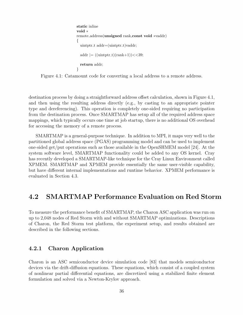
static inlinevoid ∗remote address(unsigned rank,const void ∗vaddr){

uintptr t addr=(uintptr t)vaddr;

addr |= ((uintptr t)(rank+1))<<39;

return addr;}

Figure 4.1: Catamount code for converting a local address to a remote address.

destination process by doing a straightforward address offset calculation, shown in Figure 4.1,and then using the resulting address directly (e.g., by casting to an appropriate pointertype and dereferencing). This operation is completely one-sided requiring no participationfrom the destination process. Once SMARTMAP has setup all of the required address spacemappings, which typically occurs one time at job startup, there is no additional OS overheadfor accessing the memory of a remote process.

SMARTMAP is a general-purpose technique. In addition to MPI, it maps very well to thepartitioned global address space (PGAS) programming model and can be used to implementone-sided get/put operations such as those available in the OpenSHMEM model [24]. At thesystem software level, SMARTMAP functionality could be added to any OS kernel. Crayhas recently developed a SMARTMAP-like technique for the Cray Linux Environment calledXPMEM. SMARTMAP and XPMEM provide essentially the same user-visible capability,but have different internal implementations and runtime behavior. XPMEM performance isevaluated in Section 4.3.

4.2 SMARTMAP Performance Evaluation on Red Storm

To measure the performance benefit of SMARTMAP, the Charon ASC application was run onup to 2,048 nodes of Red Storm with and without SMARTMAP optimizations. Descriptionsof Charon, the Red Storm test platform, the experiment setup, and results obtained aredescribed in the following sections.

4.2.1 Charon Application

Charon is an ASC semiconductor device simulation code [83] that models semiconductordevices via the drift-diffusion equations. These equations, which consist of a coupled systemof nonlinear partial differential equations, are discretized using a stabilized finite elementformulation and solved via a Newton-Krylov approach.

36

Charon has been designed to run on distributed memory massively parallel computersand uses MPI for all communication. Previous empirical observations have shown Charonto make MPI collective calls at high rate, and that collective performance is a major factorconstraining its performance on a large number of processors [117]. This makes Charona good candidate for performance and scalability improvement by SMARTMAP-optimizedMPI collectives.

4.2.2 Red Storm Test Platform and System Software

Red Storm is the first instance of the Cray XT architecture, and was jointly designed byCray Inc. and Sandia. At the time of the experiment, Red Storm contained a mix of dualand quad-core compute nodes, but only quad-core processors were used for testing.

Red Storm runs the Catamount operating system on its compute nodes, which is aspecial-purpose lightweight kernel designed to maximize performance for large-scale ASCapplications. The Catamount OS kernel was modified by Sandia to support SMARTMAP,and this version of Catamount has been running in production for over a year.

The Red Storm MPI library was extended by Sandia to take advantage of the SMARTMAPoptimizations for both intra-node point-to-point and collective operations. In the case of col-lective operations, a hierarchical approach is used where the first step is to perform the col-lective within each multi-core node using SMARTMAP, then one representative from eachnode communicates off-node to complete the inter-node portion of the collective. WhenSMARTMAP collectives are turned off, the MPI library uses shared-memory for MPI mes-sages sent between cores on the same node, which is more efficient than using the networkinterface in loop-back mode, but less efficient than using SMARTMAP.

4.2.3 Experiment Setup

The Charon input problem solved was to find a 2D steady-state drift-diffusion solution fora bipolar junction transistor. The Charon application code was not modified in any way.The only difference between runs was enabling or disabling SMARTMAP optimizations inthe MPI library.

Three different problem sizes were evaluated: 128, 512, and 2048 nodes. In each case,four MPI processes per node were used binding one process to each of the quad-core node’scores, resulting in 512, 2048, and 8192 total cores being used for each problem size. TheCharon input problem was scaled so that each core had about 31,000 unknowns per corefor each configuration. Dedicated system time was used to eliminate interference with otherrunning jobs. One job at a time was run, ensuring predictable allocation of nodes.

37

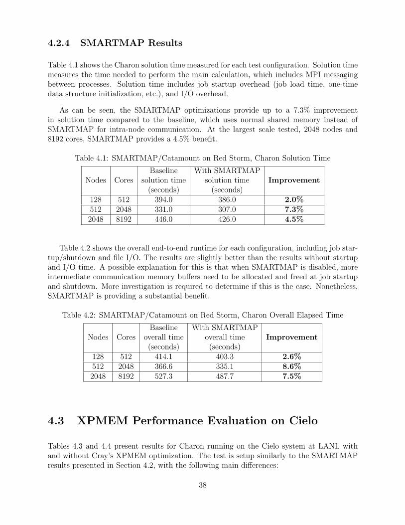
4.2.4 SMARTMAP Results

Table 4.1 shows the Charon solution time measured for each test configuration. Solution timemeasures the time needed to perform the main calculation, which includes MPI messagingbetween processes. Solution time includes job startup overhead (job load time, one-timedata structure initialization, etc.), and I/O overhead.

As can be seen, the SMARTMAP optimizations provide up to a 7.3% improvementin solution time compared to the baseline, which uses normal shared memory instead ofSMARTMAP for intra-node communication. At the largest scale tested, 2048 nodes and8192 cores, SMARTMAP provides a 4.5% benefit.

Table 4.1: SMARTMAP/Catamount on Red Storm, Charon Solution Time

Baseline With SMARTMAPNodes Cores solution time solution time Improvement

(seconds) (seconds)128 512 394.0 386.0 2.0%512 2048 331.0 307.0 7.3%2048 8192 446.0 426.0 4.5%

Table 4.2 shows the overall end-to-end runtime for each configuration, including job star-tup/shutdown and file I/O. The results are slightly better than the results without startupand I/O time. A possible explanation for this is that when SMARTMAP is disabled, moreintermediate communication memory buffers need to be allocated and freed at job startupand shutdown. More investigation is required to determine if this is the case. Nonetheless,SMARTMAP is providing a substantial benefit.

Table 4.2: SMARTMAP/Catamount on Red Storm, Charon Overall Elapsed Time

Baseline With SMARTMAPNodes Cores overall time overall time Improvement

(seconds) (seconds)128 512 414.1 403.3 2.6%512 2048 366.6 335.1 8.6%2048 8192 527.3 487.7 7.5%

4.3 XPMEM Performance Evaluation on Cielo

Tables 4.3 and 4.4 present results for Charon running on the Cielo system at LANL withand without Cray’s XPMEM optimization. The test is setup similarly to the SMARTMAPresults presented in Section 4.2, with the following main differences:

38

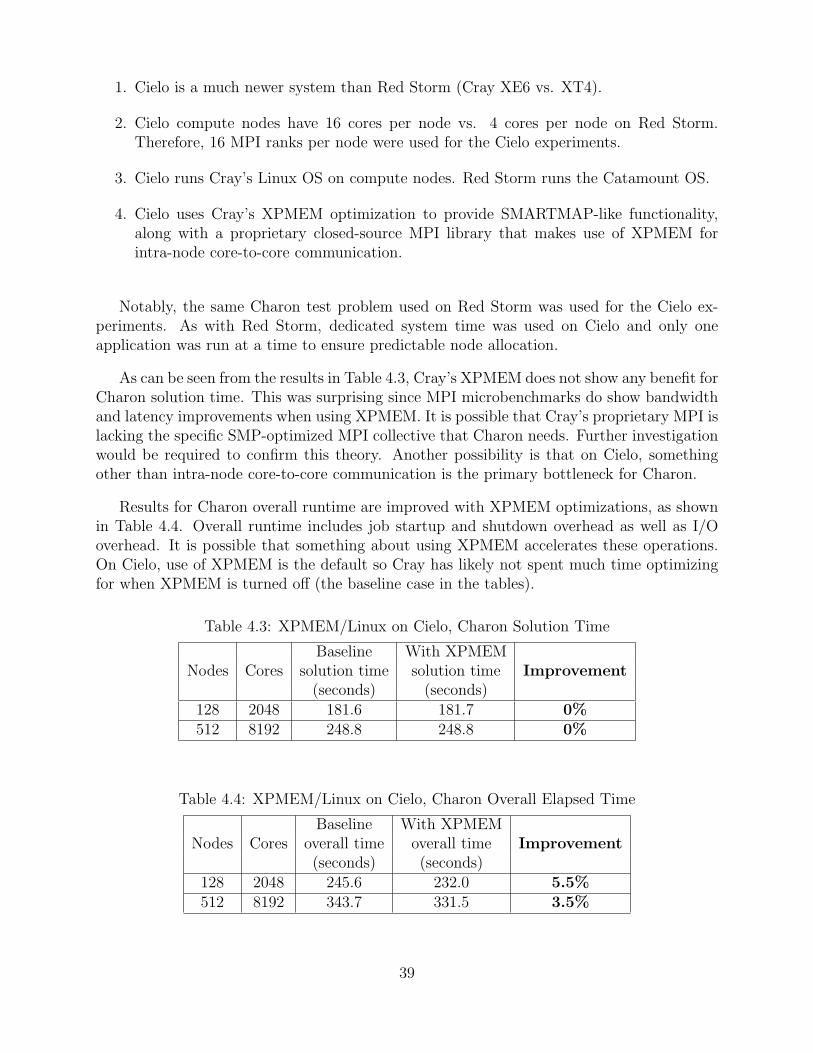
1. Cielo is a much newer system than Red Storm (Cray XE6 vs. XT4).

2. Cielo compute nodes have 16 cores per node vs. 4 cores per node on Red Storm.Therefore, 16 MPI ranks per node were used for the Cielo experiments.

3. Cielo runs Cray’s Linux OS on compute nodes. Red Storm runs the Catamount OS.

4. Cielo uses Cray’s XPMEM optimization to provide SMARTMAP-like functionality,along with a proprietary closed-source MPI library that makes use of XPMEM forintra-node core-to-core communication.

Notably, the same Charon test problem used on Red Storm was used for the Cielo ex-periments. As with Red Storm, dedicated system time was used on Cielo and only oneapplication was run at a time to ensure predictable node allocation.

As can be seen from the results in Table 4.3, Cray’s XPMEM does not show any benefit forCharon solution time. This was surprising since MPI microbenchmarks do show bandwidthand latency improvements when using XPMEM. It is possible that Cray’s proprietary MPI islacking the specific SMP-optimized MPI collective that Charon needs. Further investigationwould be required to confirm this theory. Another possibility is that on Cielo, somethingother than intra-node core-to-core communication is the primary bottleneck for Charon.

Results for Charon overall runtime are improved with XPMEM optimizations, as shownin Table 4.4. Overall runtime includes job startup and shutdown overhead as well as I/Ooverhead. It is possible that something about using XPMEM accelerates these operations.On Cielo, use of XPMEM is the default so Cray has likely not spent much time optimizingfor when XPMEM is turned off (the baseline case in the tables).

Table 4.3: XPMEM/Linux on Cielo, Charon Solution Time

Baseline With XPMEMNodes Cores solution time solution time Improvement

(seconds) (seconds)128 2048 181.6 181.7 0%512 8192 248.8 248.8 0%

Table 4.4: XPMEM/Linux on Cielo, Charon Overall Elapsed Time

Baseline With XPMEMNodes Cores overall time overall time Improvement

(seconds) (seconds)128 2048 245.6 232.0 5.5%512 8192 343.7 331.5 3.5%

39

4.4 Conclusion

The impact of SMARTMAP has been demonstrated by benchmarking the Charon semicon-ductor device simulation application running on Red Storm with and without SMARTMAPoptimizations. Results show that SMARTMAP provides a 4.5% improvement to solutiontime and a 7.5% improvement to overall elapsed time when running Charon on 2,048 quad-core compute nodes (8,192 cores) of Red Storm. Results on Cielo using Cray’s XPMEMoptimization, which provides functionality similar to SMARTMAP, are less encouraging.XPMEM provided 0% benefit to Charon solution time and 3.5% improvement to overallelapsed time on 512 Cielo compute nodes (8192 cores). SMARTMAP-like techniques suchas XPMEM should in theory provide increased benefit as the number of cores per node isincreased, since they reduce memory bandwidth, so the XPMEM results were surprising. Apossible next step is to run SMARTMAP/Catamount on Cielo to see if a larger performancebenefit is observed.

40

Chapter 5

Smart Allocation Algorithms

Abstract: Enhancements to processor allocation that enable improved job throughput aredescribed here. Experiments are described that demonstrate improvement in stream runningtime using actual job mix samples from Red Storm whose running times were scaled downto fit our test windows on Red Storm and Cielo. While improvement was demonstratedon both Red Storm and Cielo, the magnitude of the improvement seems to increase withrunning time. The magnitude of the improvement increased by tenfold when the average jobrunning time of the sample increased by less than twenty percent. This is consistent withour previous result of over twenty percent improvement on a stream of jobs that took severalhours to run on a smaller machine.

5.1 Background and Motivation

Previous experiments have shown that allocating nearby processors to each job can improvethroughput on a range of architectures [13, 95, 86, 80, 138]. The quality of an allocation canhave a significant effect on job running time; previous work has shown that hand-placinga pair of high-communication jobs into a high-contention configuration can roughly doubletheir running times [80]. The placement of job tasks has also been shown to speed up anactual application by up to 1.64 times [62]. Furthermore, with the exponential growth inthe number of cores on chips, high-quality processor allocation of cores will be necessary forgood performance on mesh-connected chips (e.g. [10]) as well.

Several papers suggest that minimizing the average number of communication hops is anappropriate metric for job placement [76, 86]. This metric was experimentally shown to cor-relate with running times by Leung et al. [80]. Krumke et al. [76] considered a generalizationof this problem on arbitrary topologies for several measures of “locality”, motivated by allo-cation on the CM5. They prove it is NP-hard to approximate average pairwise distance ingeneral. We survey approximation algorithms in Subsection 5.1.1. In previous experiments,Walker et al. [137] used the simplest of these approximation algorithms, MC1x1 (see Figure5.1(b)), to benchmark some of the heuristic algorithms surveyed in Subsection 5.1.2.

For square meshes, Walker et al. [137] find that a 1D curve-based strategy using a Hilbertcurve (see Figure 5.2(b)) can give allocations of comparable quality to a fully 2D algorithm,

41

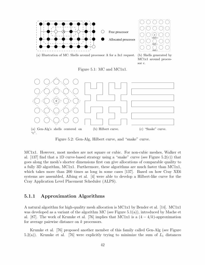
A Free processor

Allocated processor

(a) Illustration of MC: Shells around processor A for a 3x1 request.

cShell 0

Shell 1

Shell 2

(b) Shells generated byMC1x1 around proces-sor c.

Figure 5.1: MC and MC1x1.

c

(a) Gen-Alg’s shells centered on“c”.

(b) Hilbert curve. (c) “Snake” curve.

Figure 5.2: Gen-Alg, Hilbert curve, and “snake” curve.

MC1x1. However, most meshes are not square or cubic. For non-cubic meshes, Walker etal. [137] find that a 1D curve-based strategy using a “snake” curve (see Figure 5.2(c)) thatgoes along the mesh’s shorter dimensions first can give allocations of comparable quality toa fully 3D algorithm, MC1x1. Furthermore, these algorithms are much faster than MC1x1,which takes more than 200 times as long in some cases [137]. Based on how Cray XE6systems are assembled, Albing et al. [4] were able to develop a Hilbert-like curve for theCray Application Level Placement Scheduler (ALPS).

5.1.1 Approximation Algorithms

A natural algorithm for high-quality mesh allocation is MC1x1 by Bender et al. [14]. MC1x1was developed as a variant of the algorithm MC (see Figure 5.1(a)), introduced by Mache etal. [87]. The work of Krumke et al. [76] implies that MC1x1 is a (4 − 4/k)-approximationfor average pairwise distance on k processors.

Krumke et al. [76] proposed another member of this family called Gen-Alg (see Figure5.2(a)). Krumke et al. [76] were explicitly trying to minimize the sum of L1 distances

42

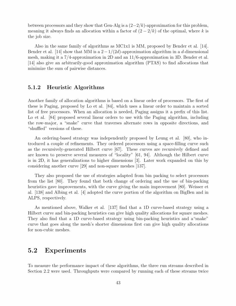
between processors and they show that Gen-Alg is a (2−2/k)-approximation for this problem,meaning it always finds an allocation within a factor of (2− 2/k) of the optimal, where k isthe job size.

Also in the same family of algorithms as MC1x1 is MM, proposed by Bender et al. [14].Bender et al. [14] show that MM is a 2−1/(2d)-approximation algorithm in a d-dimensionalmesh, making it a 7/4-approximation in 2D and an 11/6-approximation in 3D. Bender et al.[14] also give an arbitrarily-good approximation algorithm (PTAS) to find allocations thatminimize the sum of pairwise distances.

5.1.2 Heuristic Algorithms

Another family of allocation algorithms is based on a linear order of processors. The first ofthese is Paging, proposed by Lo et al. [84], which uses a linear order to maintain a sortedlist of free processors. When an allocation is needed, Paging assigns it a prefix of this list.Lo et al. [84] proposed several linear orders to use with the Paging algorithm, includingthe row-major, a “snake” curve that traverses alternate rows in opposite directions, and“shuffled” versions of these.

An ordering-based strategy was independently proposed by Leung et al. [80], who in-troduced a couple of refinements. They ordered processors using a space-filling curve suchas the recursively-generated Hilbert curve [67]. These curves are recursively defined andare known to preserve several measures of “locality” [61, 94]. Although the Hilbert curveis in 2D, it has generalizations to higher dimensions [3]. Later work expanded on this byconsidering another curve [29] and non-square meshes [137].

They also proposed the use of strategies adapted from bin packing to select processorsfrom the list [80]. They found that both change of ordering and the use of bin-packingheuristics gave improvements, with the curve giving the main improvement [80]. Weisser etal. [138] and Albing et al. [4] adopted the curve portion of the algorithm on BigBen and inALPS, respectively.

As mentioned above, Walker et al. [137] find that a 1D curve-based strategy using aHilbert curve and bin-packing heuristics can give high quality allocations for square meshes.They also find that a 1D curve-based strategy using bin-packing heuristics and a“snake”curve that goes along the mesh’s shorter dimensions first can give high quality allocationsfor non-cubic meshes.

5.2 Experiments

To measure the performance impact of these algorithms, the three run streams described inSection 2.2 were used. Throughputs were compared by running each of these streams twice

43

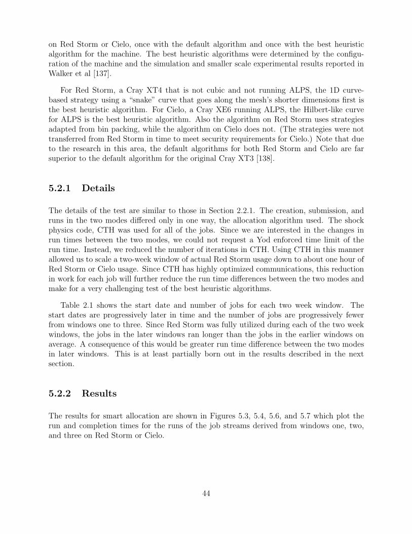
on Red Storm or Cielo, once with the default algorithm and once with the best heuristicalgorithm for the machine. The best heuristic algorithms were determined by the configu-ration of the machine and the simulation and smaller scale experimental results reported inWalker et al [137].

For Red Storm, a Cray XT4 that is not cubic and not running ALPS, the 1D curve-based strategy using a “snake” curve that goes along the mesh’s shorter dimensions first isthe best heuristic algorithm. For Cielo, a Cray XE6 running ALPS, the Hilbert-like curvefor ALPS is the best heuristic algorithm. Also the algorithm on Red Storm uses strategiesadapted from bin packing, while the algorithm on Cielo does not. (The strategies were nottransferred from Red Storm in time to meet security requirements for Cielo.) Note that dueto the research in this area, the default algorithms for both Red Storm and Cielo are farsuperior to the default algorithm for the original Cray XT3 [138].

5.2.1 Details

The details of the test are similar to those in Section 2.2.1. The creation, submission, andruns in the two modes differed only in one way, the allocation algorithm used. The shockphysics code, CTH was used for all of the jobs. Since we are interested in the changes inrun times between the two modes, we could not request a Yod enforced time limit of therun time. Instead, we reduced the number of iterations in CTH. Using CTH in this mannerallowed us to scale a two-week window of actual Red Storm usage down to about one hour ofRed Storm or Cielo usage. Since CTH has highly optimized communications, this reductionin work for each job will further reduce the run time differences between the two modes andmake for a very challenging test of the best heuristic algorithms.

Table 2.1 shows the start date and number of jobs for each two week window. Thestart dates are progressively later in time and the number of jobs are progressively fewerfrom windows one to three. Since Red Storm was fully utilized during each of the two weekwindows, the jobs in the later windows ran longer than the jobs in the earlier windows onaverage. A consequence of this would be greater run time difference between the two modesin later windows. This is at least partially born out in the results described in the nextsection.

5.2.2 Results

The results for smart allocation are shown in Figures 5.3, 5.4, 5.6, and 5.7 which plot therun and completion times for the runs of the job streams derived from windows one, two,and three on Red Storm or Cielo.

44

50

60

70

80

90

100

110

120

130

140

150

0 50 100 150 200 250 300 350

time

(sec

onds

)

job

short snake with packingdefault

(a) run times

0

500

1000

1500

2000

2500

3000

3500

4000

0 50 100 150 200 250 300 350

time

(sec

onds

)

job

short snake with packingdefault

(b) completion times

Figure 5.3: The run and completion times for the runs of the job stream derived from window one on Red Storm.

45

60

80

100

120

140

160

180

200

220

0 50 100 150 200 250 300

time

(sec

onds

)

job

short snake with packingdefault

(a) run times

0

500

1000

1500

2000

2500

3000

3500

4000

0 50 100 150 200 250 300

time

(sec

onds

)

job

short snake with packingdefault

(b) completion times

Figure 5.4: The run and completion times for the runs of the job stream derived from window two on Red Storm.

46

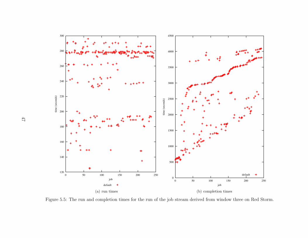
120

140

160

180

200

220

240

260

280

300

0 50 100 150 200 250

time

(sec

onds

)

job

default

(a) run times

0

500

1000

1500

2000

2500

3000

3500

4000

4500

0 50 100 150 200 250

time

(sec

onds

)

job

default

(b) completion times

Figure 5.5: The run and completion times for the run of the job stream derived from window three on Red Storm.

47

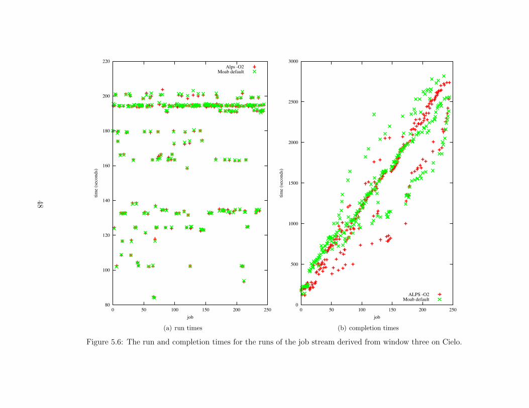
80

100

120

140

160

180

200

220

0 50 100 150 200 250

time

(sec

onds

)

job

Alps -O2Moab default

(a) run times

0

500

1000

1500

2000

2500

3000

0 50 100 150 200 250

time

(sec

onds

)

job

ALPS -O2Moab default

(b) completion times

Figure 5.6: The run and completion times for the runs of the job stream derived from window three on Cielo.

48

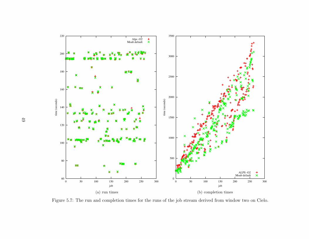
60

80

100

120

140

160

180

200

220

0 50 100 150 200 250 300

time

(sec

onds

)

job

Alps -O2Moab default

(a) run times

0

500

1000

1500

2000

2500

3000

3500

0 50 100 150 200 250 300

time

(sec

onds

)

job

ALPS -O2Moab default

(b) completion times

Figure 5.7: The run and completion times for the runs of the job stream derived from window two on Cielo.

49

5.2.2.1 Red Storm

Figure 5.3 shows the run and completion times for the runs of the job stream derive fromwindow one on Red Storm. The completion time for a job is determined by both when it isscheduled and how it is allocated. Since both the schedule and allocation differed betweenthe two runs, we compared the run time for each job and the job stream as a whole. Seventy-one jobs took less time, ninety-six jobs took about the same amount of time, and 155 jobstook more time with the best heuristic algorithm. Overall, it takes approximately 0.33% lesstime for the stream to run with the best heuristic algorithm. As noted above, the researchin this area have improved the default algorithm on Red Storm, and the use of CTH andthe reduction in work for each job would reduce the run time differences between the twomodes.

Figure 5.4 shows the run and completion times for the runs of the job stream derive fromwindow two on Red Storm. Ninety jobs took less time, seventy-eight jobs took about thesame amount of time, and ninety-six jobs took more time with the best heuristic algorithm.Overall, it takes approximately three percent less time for the stream to run with the bestheuristic algorithm. Note that window two with fewer jobs takes about the same time to runas window one. Therefore the jobs in window two must take on average more time to run.This difference could account for the greater separation between the two modes for windowtwo.

Figure 5.5 shows that window three has fewer jobs than window two and took longer torun in the default mode. Unfortunately the experiments on Red Storm were not withoutsome minor glitches, and we ran out of time before we could run window three with the bestheuristic algorithm. So we ran the Cielo experiments in the reverse order.

5.2.2.2 Cielo

Figure 5.6 shows the run and completion times for the runs of the job stream derive fromwindow three on Cielo. 161 jobs took less time and eighty-four jobs took more time withthe best heuristic algorithm. Overall, it takes approximately three percent less time for thestream to run with the best heuristic algorithm. This is the same percentage difference forwindow two on Red Storm. Note that this job stream took less time to run on Cielo than itdid on Red Storm. The job stream derived from a Red Storm window appears not to haveposed a similar challenge to Cielo, a couple of generations beyond Red Storm.

Figure 5.7 shows the run and completion times for the runs of the job stream derive fromwindow two on Cielo. 173 jobs took less time, and ninety-one jobs took more time with theheuristic algorithm. Overall, it takes approximately six percent more time for the stream torun with the heuristic algorithm. Note that the run times for the jobs in windows two andthree seem to be fairly consistent on Cielo. This could explain the relationship between thetimes for windows two and three being reversed on Cielo, i.e. the time for window three wasless than the time for window two. However, it is not clear why the performance of the best

50

heuristic algorithm flipped between the two windows.

We were able to run only two windows for both the default and best heuristic algorithmin the time allotted on Cielo. Therefore, the only overlaps between the runs on Red Stormand the runs on Cielo were for window two and part of window three. Note that the jobswere scheduled differently on Red Storm and Cielo. The scheduler on Red Storm selects thelargest job possible, while the scheduler on Cielo does not. It is not clear whether this is aconsequential difference.

5.3 Conclusions

Due to the research in this area, the default algorithms for both Red Storm and Cielo arefar superior to the default algorithms for the original Cray XT3 [138]. Additionally, the useof CTH with its optimized communications and the reduction in its run time to fit into ourtest window made for a very challenging test for our best heuristic algorithms. Despite thesevery challenging conditions, the best heuristic algorithms were able to show improvementsover the default algorithms on Red Storm and Cielo. This was especially true for longerrunning jobs. For both Red Storm and Cielo, the longer running jobs in the later windowsyielded better results for the best heuristic algorithms. For example, both the 322 jobs inwindow one and the 264 jobs in window two took about an hour to run on Red Storm,but the percentage improvement of the best heuristic algorithm increased by a factor of tenfrom window one to window two. This is not inconsistent with our previous result of overtwenty percent improvement on a stream of jobs that took several hours to run on a smallermachine [80]. The advantage of the best heuristic algorithm seems to increase for longerrunning jobs.

51

52

Chapter 6

Enhancements to Red Storm andCatamount to Increase PowerEfficiency During ApplicationExecution

Abstract: In the scientific High Performance Computing sector, run-time performance hasbeen the primary, if not sole, metric for measuring success. Recently, however, the impor-tance of power as a metric has been recognized and new multi-dimensioned metrics are beingconsidered such as; FLOPs per Watt and energy or cost to solution. We have addressed thischanging priority by demonstrating that power efficiency can be achieved with little to noimpact on performance. Our experiments have shown that increased power efficiency canbe gained by exploiting existing bottle-necks in scientific applications. In a series of experi-ments, we characterize the effect of both CPU frequency and network bandwidth tuning onpower usage and demonstrate energy savings of up to 39% with little to no impact on run-time performance. These results on existing platforms indicate next generation large-scaleplatforms should not only approach CPU frequency scaling differently, but could also bene-fit from the capability to tune other platform components, such as the network, to achievegreater energy efficiency. Our results also indicate that there are significant opportunities forthis work to impact how future algorithms are implemented to maximize both performanceand energy efficiency.

6.1 Introduction and Motivation

Power has increasingly been identified as the tall pole in the path to Exascale. Applicationsexecuting on next generation systems will not only have to meet performance goals butaccomplish these goals within an environment that will possibly diverge greatly from currentplatforms. It is clear that one of our future challenges will be increasing energy efficiencywhile preserving application performance. Our motivation for this work is to demonstrateimprovements in energy efficiency using current ASC scientific applications on existing ASCplatforms. Our experiments will not only reveal where energy efficiency can be increased butwhat software and hardware platform characteristics will have the most impact, if available,

53

on future ASC platforms.

In response to this challenge we apply a, thus far, unique ability to measure current drawand voltage, in situ, to analyze the trade-offs between performance and energy efficiency ofproduction ASC scientific applications run at large scale (thousands of nodes) while manip-ulating CPU frequency and network bandwidth.

The results of our experiments clearly indicate that opportunities exist to save energyby tuning platform components without sacrificing application performance. Our goal is toreduce energy consumption of scientific applications run at very large scale while minimizingthe impact on run-time performance (wall-clock execution time).

Evaluating acceptable trade-offs between energy efficiency and run-time performance is,of course, somewhat subjective. Our work indicates that the parameters of these trade-offsare application dependent. With annual power costs on track to meet or exceed acquisitioncosts of next generation large scale platforms, our traditional prioritization of performanceabove all will be forced to change. It is likely that more emphasis will be placed on energy ef-ficiency metrics like FLOPS/Watt, Energy Delay Product or energy to solution. Regardless,performance remains a critical parameter of our evaluation.

6.2 CPU Frequency Tuning

Typical approaches to CPU frequency scaling employed by operating systems, such as Linux,while efficient for single server or laptop implementations, have proven to be detrimentalwhen used at scale causing the equivalent of operating system jitter[113]. For this reason, itis common practice at most HPC sites that deploy medium to large scale clusters to disablefrequency scaling. It is clear to us that techniques designed for laptop energy efficiency arenot directly applicable to large scale HPC platforms. It is particularly important that anyapproach taken has a system-level, rather than node-level, view of these issues.

To accomplish our goals, we made a small number of targeted modifications to the Cata-mount light-weight kernel. Typically, light-weight kernels are small and accommodate lowlevel changes more easily than general purpose operating systems, such as Linux. Ourchanges to Catamount involved leveraging the Dynamic Voltage and Frequency Scaling(DVFS) capabilities available on the processor (CPU). We made additions to Catamount thatallowed a user space process to request a CPU frequency change. Currently, our methodof frequency scaling is limited to frequencies defined in the P-state table, although mostprocessors support frequency stepping in 100MHz increments.

Power on CMOS chips has three primary contributing factors; dynamic power, staticpower and leakage current. Equation 6.1 depicts each contributing factor.

54

P = dynamicP + staticP + leakageI

P = ACV 2f + tAV Ishortf + V Ileak (6.1)

Dynamic power currently dominates the equation, but leakage current is quickly becominga significant contributor. We will focus on the contribution of dynamic power. Notice, thereis a quadratic relationship between voltage (V) and power (P). Consequently, the largestimpact on power can be obtained by lowering input voltage which is what our frequencychanges ultimately accomplish.

In our CPU frequency experiments we employ static frequency scaling. Static frequencyscaling is defined, for our purposes, as changing the processor frequency to a specified stateand keeping that frequency state constant over the duration of the application execution.The applications used in our experiments were selected based on their importance to thethree DOE National Nuclear Security Administration (NNSA) nuclear weapons laboratories(Sandia, Los Alamos and Lawrence Livermore). The test applications include; SAGE, CTH,AMG2006, xNOBEL, UMT, Charon and LAMMPS. We tested each application at a rangeof frequencies (P-states) and measured the energy used over the duration of the applicationexecution.

Decreasing CPU frequency, in general, will slow active computation. If applicationswere solely gated by computation this approach would be entirely detrimental. However,applications exhibit a range of characteristics. In this experiment, we altered CPU frequencyand measured the impact on CPU energy and run-time (other platform parameters are leftunchanged). Note, for all experiments we contrast both run-time and CPU energy to thebaseline runs conducted at P-states 0 or 1 (depending on the platform used) and report thecontrast as percent difference. For the baseline runs we record the execution time in seconds(s) and the energy used in Joules (J).

Our CPU frequency experiments focused on the effect that CPU frequency modificationshad on CPU energy alone. CPU energy is the single largest contributor to total node energyused as observed in [52]. On our test platforms, CPU energy ranges from 44-57% of totalnode power. For this reason we feel measuring CPU energy in isolation is important. Further,the results of this experiment have the potential to be more widely applicable. Later, wetake a broader look at total system energy in our network bandwidth tuning experiment.Total energy considers the contribution of additional node components and is somewhatmore platform specific than our CPU energy analysis. We feel both approaches have utilityand provide interesting insights.

6.2.1 Results: CPU Frequency Tuning

Table 6.1 lists the results of our CPU frequency scaling experiments. We obtained resultsfor AMG2006 at P-states 1-4 at a scale of 6K cores. At P-state 2 we observed an increase in

55

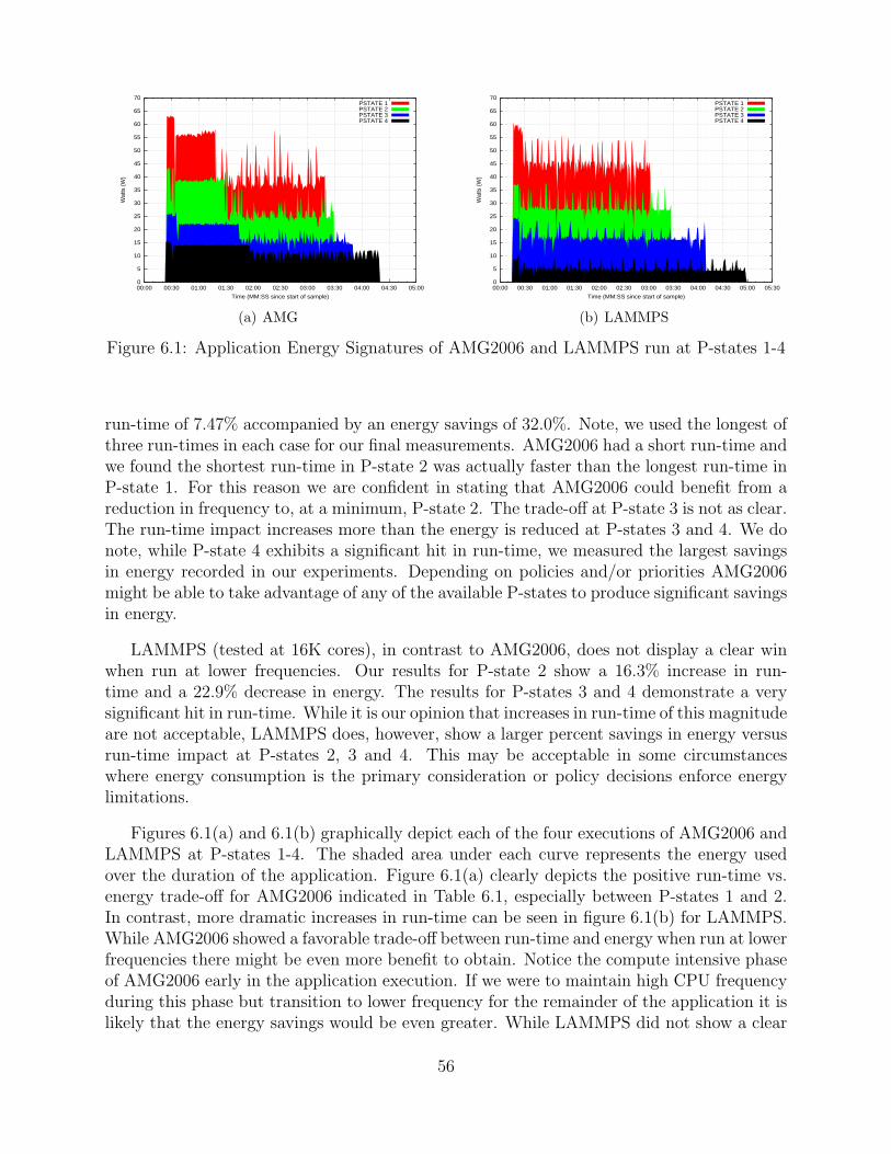
0

5

10

15

20

25

30

35

40

45

50

55

60

65

70

00:00 00:30 01:00 01:30 02:00 02:30 03:00 03:30 04:00 04:30 05:00

Wat

ts (

W)

Time (MM:SS since start of sample)

PSTATE 1PSTATE 2PSTATE 3PSTATE 4

(a) AMG

0

5

10

15

20

25

30

35

40

45

50

55

60

65

70

00:00 00:30 01:00 01:30 02:00 02:30 03:00 03:30 04:00 04:30 05:00 05:30

Wat

ts (

W)

Time (MM:SS since start of sample)

PSTATE 1PSTATE 2PSTATE 3PSTATE 4

(b) LAMMPS

Figure 6.1: Application Energy Signatures of AMG2006 and LAMMPS run at P-states 1-4

run-time of 7.47% accompanied by an energy savings of 32.0%. Note, we used the longest ofthree run-times in each case for our final measurements. AMG2006 had a short run-time andwe found the shortest run-time in P-state 2 was actually faster than the longest run-time inP-state 1. For this reason we are confident in stating that AMG2006 could benefit from areduction in frequency to, at a minimum, P-state 2. The trade-off at P-state 3 is not as clear.The run-time impact increases more than the energy is reduced at P-states 3 and 4. We donote, while P-state 4 exhibits a significant hit in run-time, we measured the largest savingsin energy recorded in our experiments. Depending on policies and/or priorities AMG2006might be able to take advantage of any of the available P-states to produce significant savingsin energy.

LAMMPS (tested at 16K cores), in contrast to AMG2006, does not display a clear winwhen run at lower frequencies. Our results for P-state 2 show a 16.3% increase in run-time and a 22.9% decrease in energy. The results for P-states 3 and 4 demonstrate a verysignificant hit in run-time. While it is our opinion that increases in run-time of this magnitudeare not acceptable, LAMMPS does, however, show a larger percent savings in energy versusrun-time impact at P-states 2, 3 and 4. This may be acceptable in some circumstanceswhere energy consumption is the primary consideration or policy decisions enforce energylimitations.

Figures 6.1(a) and 6.1(b) graphically depict each of the four executions of AMG2006 andLAMMPS at P-states 1-4. The shaded area under each curve represents the energy usedover the duration of the application. Figure 6.1(a) clearly depicts the positive run-time vs.energy trade-off for AMG2006 indicated in Table 6.1, especially between P-states 1 and 2.In contrast, more dramatic increases in run-time can be seen in figure 6.1(b) for LAMMPS.While AMG2006 showed a favorable trade-off between run-time and energy when run at lowerfrequencies there might be even more benefit to obtain. Notice the compute intensive phaseof AMG2006 early in the application execution. If we were to maintain high CPU frequencyduring this phase but transition to lower frequency for the remainder of the application it islikely that the energy savings would be even greater. While LAMMPS did not show a clear

56

win when lowering CPU frequency we observed very regular compute and communicationphases throughout the entire application execution (indicated by peaks and valleys in thegraph). We have work planned to further examine these application characteristics, andpotentially leveraged them using a more dynamic approach, to obtain power savings even inapplications that do not present a clear choice when we statically modify the CPU frequency.

We obtained results for SAGE at two different scales (4K and 16K cores). In both cases,a small increase in run-time (0.402% at larger scale and 3.86% at smaller scale) is observedaccompanied by a very significant reduction in energy (39.5% at large scale and 38.9% atsmall scale). We were able to obtain results for a 4k core run of SAGE at P-state 3. Theimpact on run-time remains low while additional energy savings were recorded. Based onour observations, it is possible that SAGE run at 16k cores would have also demonstrated afavorable trade-off at P-state 3.

CTH was executed at P-states 0, 2 and 3 at a scale of 16K cores. Similar to LAMMPS,there is no clear win with CTH when the CPU frequency is lowered. Also, like LAMMPS,CTH has very regular compute and communication phases. LAMMPS and CTH will likelyboth be targets of our future work in dynamic CPU frequency scaling at large scale.

We obtained results for xNOBEL at 6K cores at P-states 0, 2 and 3. Our results indicatethat xNOBEL, like AMG2006, is a good candidate for CPU frequency reduction. Havingthe ability to tune CPU frequency at large scale for this application is a clear win.

UMT and Charon behaved in a very similar manner. Since UMT was run at a muchlarger scale than Charon (16K cores vs. 4K cores) we feel the results obtained for UMT aremore meaningful and more accurately represent what we could expect at large scale. Charonmay act differently when run at larger scale, but these results indicate that both UMT andCharon are sensitive to CPU frequency changes. It is possible that further analysis will revealopportunities to dynamically scale frequency during the execution of these applications.

The CPU is only one component that affects application performance. In the follow-ing section we will experiment with tuning network bandwidth and observe the trade-offsbetween performance vs. total system energy.

57

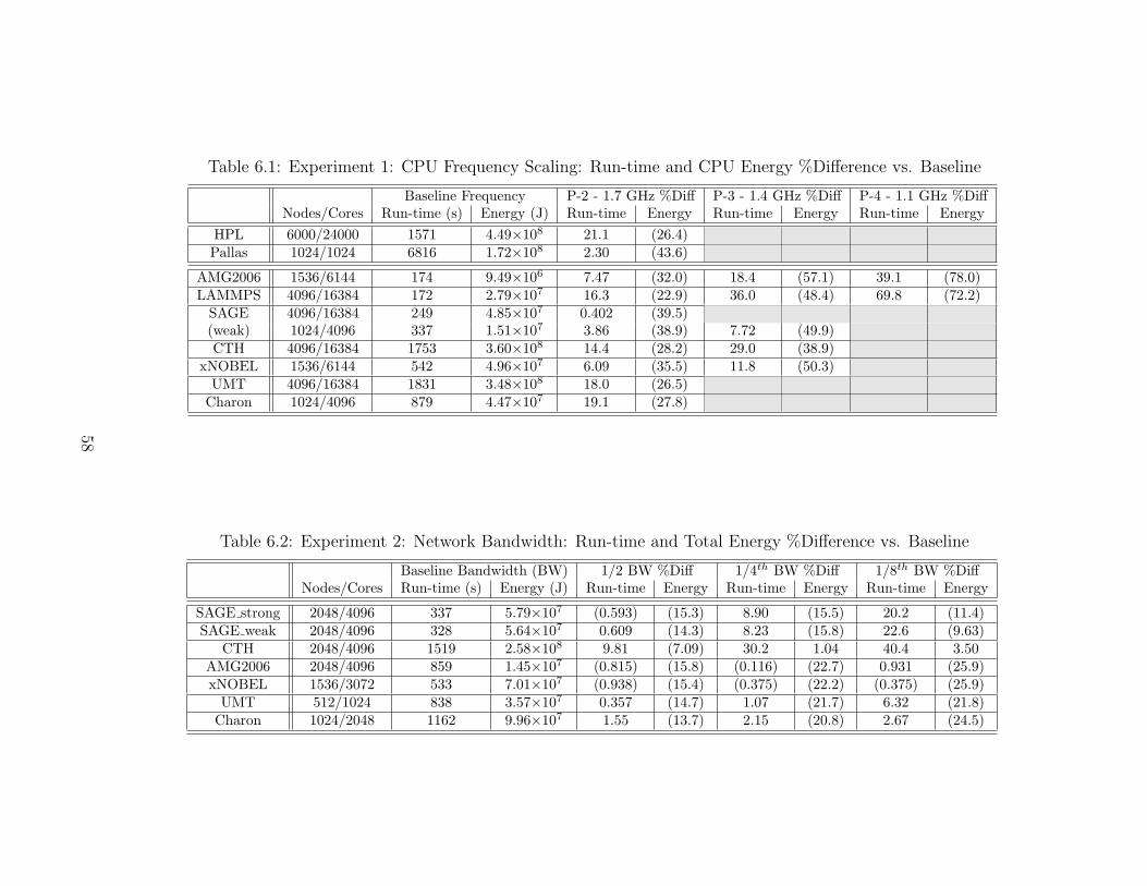
Table 6.1: Experiment 1: CPU Frequency Scaling: Run-time and CPU Energy %Difference vs. Baseline

Baseline Frequency P-2 - 1.7 GHz %Diff P-3 - 1.4 GHz %Diff P-4 - 1.1 GHz %DiffNodes/Cores Run-time (s) Energy (J) Run-time Energy Run-time Energy Run-time Energy

HPL 6000/24000 1571 4.49×108 21.1 (26.4)Pallas 1024/1024 6816 1.72×108 2.30 (43.6)

AMG2006 1536/6144 174 9.49×106 7.47 (32.0) 18.4 (57.1) 39.1 (78.0)LAMMPS 4096/16384 172 2.79×107 16.3 (22.9) 36.0 (48.4) 69.8 (72.2)

SAGE 4096/16384 249 4.85×107 0.402 (39.5)(weak) 1024/4096 337 1.51×107 3.86 (38.9) 7.72 (49.9)CTH 4096/16384 1753 3.60×108 14.4 (28.2) 29.0 (38.9)

xNOBEL 1536/6144 542 4.96×107 6.09 (35.5) 11.8 (50.3)UMT 4096/16384 1831 3.48×108 18.0 (26.5)

Charon 1024/4096 879 4.47×107 19.1 (27.8)

Table 6.2: Experiment 2: Network Bandwidth: Run-time and Total Energy %Difference vs. Baseline

Baseline Bandwidth (BW) 1/2 BW %Diff 1/4th BW %Diff 1/8th BW %DiffNodes/Cores Run-time (s) Energy (J) Run-time Energy Run-time Energy Run-time Energy

SAGE strong 2048/4096 337 5.79×107 (0.593) (15.3) 8.90 (15.5) 20.2 (11.4)SAGE weak 2048/4096 328 5.64×107 0.609 (14.3) 8.23 (15.8) 22.6 (9.63)

CTH 2048/4096 1519 2.58×108 9.81 (7.09) 30.2 1.04 40.4 3.50AMG2006 2048/4096 859 1.45×107 (0.815) (15.8) (0.116) (22.7) 0.931 (25.9)xNOBEL 1536/3072 533 7.01×107 (0.938) (15.4) (0.375) (22.2) (0.375) (25.9)

UMT 512/1024 838 3.57×107 0.357 (14.7) 1.07 (21.7) 6.32 (21.8)Charon 1024/2048 1162 9.96×107 1.55 (13.7) 2.15 (20.8) 2.67 (24.5)

58

6.3 Network Bandwidth Tuning

Our goal in this experiment was to determine the affect on run-time performance and en-ergy of production scientific applications run at very large scale while tuning the networkbandwidth of an otherwise balanced platform. To accomplish network bandwidth scalingwe employed two different tunable characteristics of the Cray XT architecture. First, wetuned the Seastar NIC to reduce the interconnect bandwidth in stages to 1/2 and 1/4th offull bandwidth. Next, we used the ability to tune the node injection bandwidth, effectivelyreducing the network bandwidth to 1/8th. This allowed for the most complete stepwisereduction in overall network bandwidth we were able to achieve using this architecture.

Modifying the network interconnect bandwidth on the Cray XT requires a fairly simplechange to the router configuration file, consulted during the routing process of the bootsequence. A full system reboot is required for every alteration of the interconnect bandwidth.Typically, all four rails of the Seastar are configured to be enabled. Alternatively, the numberof enabled rails can be reduced by specifying a bitmask in the system’s router configurationfile (e.g., 1111 for four rails, 0011 for two rails). In our experiments, we configured theinterconnect bandwidth of the Seastar to effectively tune the network bandwidth to full, 1/2and 1/4th.

Since the interconnect bandwidth on the XT architecture is far greater than the injec-tion bandwidth of an individual node, the interconnect bandwidth had to be reduced to 1/2before it produced a measurable effect. Multiple nodes may route through an individualSeastar depending on communication patterns and node placement relative to logical net-work topology. For this reason, we limited our experiments to one application executing ata time. This allowed for the nearest estimation of the impact of network bandwidth tuningon an individual application. Running other applications concurrently would be an inter-esting experiment but would greatly complicate analysis and was beyond the scope of thisexperiment but is planned for future investigations.

Tuning the node injection bandwidth, to further reduce the network bandwidth, requiresa small modification to the Cray XT bootstrap source code. Cray provided us access to thissource code under a proprietary license. The portion of the code that required modification(coldstart) serves an equivalent purpose to the BIOS on a personal computer or server. Ourexperiments were conducted in phases beginning with a baseline full bandwidth run for eachapplication followed by subsequent executions at each reduced bandwidth.

For each phase we collected power samples (current draw and voltage). The scale usedfor each application, number of nodes and cores, is listed in Table 6.2. No operating systemmodifications were necessary for either the interconnect or injection bandwidth experiments.

59

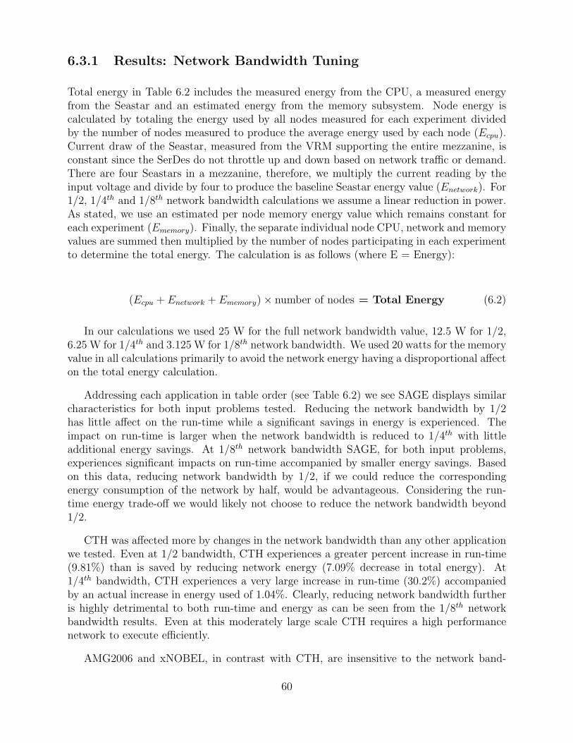
6.3.1 Results: Network Bandwidth Tuning

Total energy in Table 6.2 includes the measured energy from the CPU, a measured energyfrom the Seastar and an estimated energy from the memory subsystem. Node energy iscalculated by totaling the energy used by all nodes measured for each experiment dividedby the number of nodes measured to produce the average energy used by each node (Ecpu).Current draw of the Seastar, measured from the VRM supporting the entire mezzanine, isconstant since the SerDes do not throttle up and down based on network traffic or demand.There are four Seastars in a mezzanine, therefore, we multiply the current reading by theinput voltage and divide by four to produce the baseline Seastar energy value (Enetwork). For1/2, 1/4th and 1/8th network bandwidth calculations we assume a linear reduction in power.As stated, we use an estimated per node memory energy value which remains constant foreach experiment (Ememory). Finally, the separate individual node CPU, network and memoryvalues are summed then multiplied by the number of nodes participating in each experimentto determine the total energy. The calculation is as follows (where E = Energy):

(Ecpu + Enetwork + Ememory) × number of nodes = Total Energy (6.2)

In our calculations we used 25 W for the full network bandwidth value, 12.5 W for 1/2,6.25 W for 1/4th and 3.125 W for 1/8th network bandwidth. We used 20 watts for the memoryvalue in all calculations primarily to avoid the network energy having a disproportional affecton the total energy calculation.

Addressing each application in table order (see Table 6.2) we see SAGE displays similarcharacteristics for both input problems tested. Reducing the network bandwidth by 1/2has little affect on the run-time while a significant savings in energy is experienced. Theimpact on run-time is larger when the network bandwidth is reduced to 1/4th with littleadditional energy savings. At 1/8th network bandwidth SAGE, for both input problems,experiences significant impacts on run-time accompanied by smaller energy savings. Basedon this data, reducing network bandwidth by 1/2, if we could reduce the correspondingenergy consumption of the network by half, would be advantageous. Considering the run-time energy trade-off we would likely not choose to reduce the network bandwidth beyond1/2.

CTH was affected more by changes in the network bandwidth than any other applicationwe tested. Even at 1/2 bandwidth, CTH experiences a greater percent increase in run-time(9.81%) than is saved by reducing network energy (7.09% decrease in total energy). At1/4th bandwidth, CTH experiences a very large increase in run-time (30.2%) accompaniedby an actual increase in energy used of 1.04%. Clearly, reducing network bandwidth furtheris highly detrimental to both run-time and energy as can be seen from the 1/8th networkbandwidth results. Even at this moderately large scale CTH requires a high performancenetwork to execute efficiently.

AMG2006 and xNOBEL, in contrast with CTH, are insensitive to the network band-

60

width changes in terms of run-time, but demonstrate large energy savings opportunities.Reductions down to 1/8th network bandwidth cause virtually no impact in run-time for bothAMG2006 and xNOBEL while a 25.9% savings in energy can be achieved for both. We donote the savings in energy seems to be flattening by the time we reduce network bandwidthto 1/8th. While further reductions in network bandwidth may or may not increase run-time,there is likely little additional energy savings available.

UMT produced similar results to AMG2006 and xNOBEL when the network bandwidthwas reduced up to 1/4th, little to no impact in run-time accompanied by a large energysavings. At 1/8th network bandwidth we see different characteristics. UMT experiences amuch higher impact on run-time at 1/8th network bandwidth (6.32%) than at 1/4th (1.07%)with virtually no additional energy savings (21.7% at 1/4th and 21.8% at 1/8th). We seem tohave found the limit of network bandwidth tuning that should be applied to UMT at leastat this scale. We should note that UMT was run at a smaller scale relative to the otherapplications. It is possible that at larger scale our results would differ.

Charon showed small, but increasing, impact on run-time as we reduced network band-width. At this scale it is clear that we could reduce the network bandwidth down to 1/4th

with probably an acceptable impact in run-time (increase of 2.15%) accompanied by a verysignificant savings in energy (decrease of 20.8%). Moving from 1/4th to 1/8th network band-width shows indications that the energy savings is flattening but results are not conclusive.Experiments with Charon at larger scale are also warranted.

Overall, we observed significant evidence that a tunable network would be beneficial formost of the applications tested. In all cases but CTH, virtually no impact to run-time wouldbe experienced by tuning the network bandwidth to 1/2. The result would be significantenergy savings with little to no performance impact. In the case of AMG2006, xNOBEL andUMT the network bandwidth could be reduced to 1/4th full bandwidth with little run-timeimpact, allowing for even larger energy savings. Our observations indicate that a tunablenetwork would be beneficial but they also indicate a high performance network is critical forsome applications. The ability to tune the network, similar to how frequency is tunable ona CPU, would be an important characteristic on next generation exascale platforms.

It should be stressed that our data is representative of a single application running at atime. One of the reasons the interconnect bandwidth of the Seastar was designed to be greaterthan the injection bandwidth of a single node is that the network is a shared resource on theCray XT architecture, shared by all simultaneously running applications. Often many hopsare required for a messages to travel from source to destination, and poor node mappingsresult in individual network links carrying messages for multiple applications. Having agreater interconnect bandwidth is essential for handling this increased load. Thus, the abilityto tune network performance could not be exploited without considering the possible impacton other applications running on the platform, at least for network topologies like meshesand 3D-toruses. Network topologies with fewer hops on average could benefit more easilyfrom a tunable network since less consideration would be necessary regarding the impact onother applications co-existing on the platform.

61

0

0.5

1

1.5

2.0

P0/1 P2 P3 P4

2.2MHz 1.7 MHz 1.4 MHz 1.1 MHzN

OR

MA

LIZ

ED

to d

efa

ult P

sta

te

Processor Pstate Setting

Processor Frequency

HPL (6000)RuntimeEnergyEnergy * TimeEnergy * (Time)2

Energy * (Time)3

P0/1 P2 P3 P4

2.2MHz 1.7 MHz 1.4 MHz 1.1 MHz

AMG2006 (1536)RuntimeEnergyEnergy * TimeEnergy * (Time)2

Energy * (Time)3

P0/1 P2 P3 P4 0

0.5

1

1.5

2.02.2MHz 1.7 MHz 1.4 MHz 1.1 MHz

LAMMPS (4096)RuntimeEnergyEnergy * TimeEnergy * (Time)2

Energy * (Time)3

Figure 6.2: Normalized Energy, Run-time and (E ∗ Tw) where (w) = 1, 2, or3

6.4 Energy Delay Product

Calculating the Energy Delay Product (EDP) [69],[28] is one way of producing a singleone-dimensional metric to evaluate both the energy and performance impact. In figure 6.2we have graphed the energy and runtime normalized to baseline and three separate EDPcurves using the equation E ∗ Tw where w = 1, 2 or 3 for HPL, AMG2006 and LAMMPS.The graphs shown are based on the same data used for Table 6.1 from experiment #1. Datafrom both experiments #1 and #2 have been analyzed and while too extensive for this reportresults can be found in SAND2011-5702 in their entirety. The HPL graph demonstrates theprogressive affect increasing the exponent of the time factor has on the metric. This graphreinforces why we would likely not use an unweighted EDP calculation for HPC applications.The EDP squared and EDP cubed plots more accurately represent our previous analysis ofthe affect of lowering frequency for HPL. The graphs representing AMG and LAMMPSparallel our previous analysis nicely. Even the EDP cubed curve indicates it is beneficialto lower the CPU frequency while running AMG. In the case of LAMMPS if we basedour analysis on EDP squared we might determine there is benefit if we run at P-state 4.If we evaluate based on the EDP cubed curve all P-states are detrimental. Generally, nosignificantly different insights were discovered using EDP for analysis but they did serve asreinforcement of our initial conclusions.

6.5 Conclusions

Applications like AMG2006, and xNOBEL were fairly insensitive to CPU frequency reduc-tions. Both AMG2006 and xNOBEL were also tolerant of network bandwidth reductions.It is possible that if we tune both the CPU frequency and network bandwidth, at the sametime, we could realize even greater energy savings. As an example, if we use the per nodeenergy value for xNOBEL when executed at P-state 2 in our total energy calculation for the1/8th network bandwidth experiment, xNOBEL would experience a total of 56.4% in energysavings with a 6% impact in runtime.

62

We specifically selected xNOBEL in our previous example since it was the least impactedby any tuning we applied. CTH, however, was significantly affected by CPU frequencyadjustments. If we did choose to reduce CPU frequency, could we reduce the networkbandwidth without further impact on run-time but save additional energy making the run-time impact more palatable? Possibly, if memory or some other component is the bottleneck,but we cannot definitively state this would be the result. A better approach for applicationslike CTH would be to apply dynamic frequency scaling but coordinated with applicationcompute and communication cycles.

Our experiments indicate each application has a sweet spot based on its computationand communication requirements. Additionally, we have observed energy savings and run-time are impacted, often significantly, by scale. We feel that the trade-offs are platform andapplication specific – when one bottleneck is removed, another will appear, and the orderthat the bottlenecks appear will depend on the platform. Conducting these experiments ona platform like the Cray XT is valuable since it is a well-balanced in its default configuration.As a result of our experiments, we have concluded that components on future HPC platforms(exascale and beyond) should be as tunable as possible under software control so that end-users or system software can optimize the energy/performance trade-off.

63

64

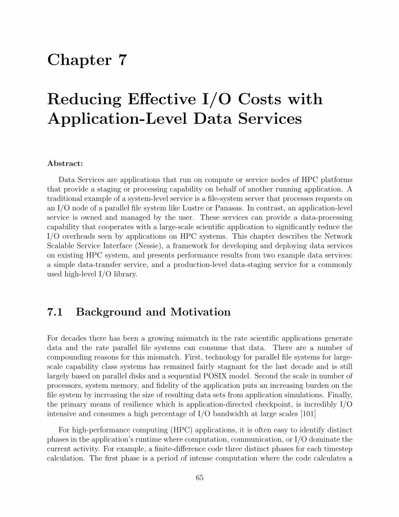
Chapter 7

Reducing Effective I/O Costs withApplication-Level Data Services

Abstract:

Data Services are applications that run on compute or service nodes of HPC platformsthat provide a staging or processing capability on behalf of another running application. Atraditional example of a system-level service is a file-system server that processes requests onan I/O node of a parallel file system like Lustre or Panasas. In contrast, an application-levelservice is owned and managed by the user. These services can provide a data-processingcapability that cooperates with a large-scale scientific application to significantly reduce theI/O overheads seen by applications on HPC systems. This chapter describes the NetworkScalable Service Interface (Nessie), a framework for developing and deploying data serviceson existing HPC system, and presents performance results from two example data services:a simple data-transfer service, and a production-level data-staging service for a commonlyused high-level I/O library.

7.1 Background and Motivation

For decades there has been a growing mismatch in the rate scientific applications generatedata and the rate parallel file systems can consume that data. There are a number ofcompounding reasons for this mismatch. First, technology for parallel file systems for large-scale capability class systems has remained fairly stagnant for the last decade and is stilllargely based on parallel disks and a sequential POSIX model. Second the scale in number ofprocessors, system memory, and fidelity of the application puts an increasing burden on thefile system by increasing the size of resulting data sets from application simulations. Finally,the primary means of resilience which is application-directed checkpoint, is incredibly I/Ointensive and consumes a high percentage of I/O bandwidth at large scales [101]

For high-performance computing (HPC) applications, it is often easy to identify distinctphases in the application’s runtime where computation, communication, or I/O dominate thecurrent activity. For example, a finite-difference code three distinct phases for each timestepcalculation. The first phase is a period of intense computation where the code calculates a

65

resulting value for a particular data point based on a function applied to its nearest neigh-bors. After the compute-intensive phase, there is a period of intense communication whereprocessor boundary values are exchanged with other processors in the parallel application.Finally, at the end of the communication-intensive phase for some of the timestep calcula-tions, there is an I/O-intensive phase where the application writes a (perhaps large) portionof its memory to the file system as a “restart” file allowing the application to make progressin the event of an application or system failure.

Of the three phases, I/O is often the largest performance bottleneck for the application.While there are known techniques for overlapping communication and computation (e.g.,double buffering and asynchronous message passing), the I/O cost is difficult to hide. Usingtraditional POSIX interfaces, the majority of the application is idle while data streams frommemory to the remote storage devices. Efforts to make the I/O phase asynchronous requirelarge local memory reserves and have often led to unexpected interference effects that furtherreduce application performance [1].

One approach to both reduce the burden on the file system and improve “effective” I/Orates for the application is to employ the use of “data services” [1, 85, 97, 100, 139]. Simplyput, a data service is a separate (possibly parallel) application that performs operationson behalf of an actively running scientific application. This type of processing was firstdemonstrated for HPC computing as part of the Salvo seismic imaging application in mid1990s [106]. Salvo used an “I/O Partition” to perform preprocessing (FFTs) on data betweenthe storage systems and the application. As HPC systems continued to evolve, the need tosupplement parallel file systems with similar approaches became evident. Now there areentire research communities exploring better ways to use similar processing techniques fordata staging and in-situ analysis.

A data service architecture uses remote direct-memory access (RDMA) to move data frommemory to memory between the application and the service(s). Figure 7.1 illustrates theorganization of an application using data services. On current capability-class HPC systems,services execute on compute nodes or service nodes and provide the application the ability to“offload” operations that present scalability challenges for the scientific code. One commonlyused example for data services is data staging, or caching data between the application andthe storage system [100, 101, 118]. Section 7.4 describes such a service. Other examplesinclude proxies for database operations [105] and in-situ data analysis [57, 85, 139].

This chapter provides a description of our data-service framework the Network ScalableService Interfaice (Nessie), as well as examples and performance results of data services cur-rently in use or in development at Sandia. The data-transfer service, described in Section 7.3,is the canonical example on how to develop a data service using Nessie, and the PnetCDFservice from Section 7.4 is an example of link-time replacement I/O library that performsdata-staging for bursty I/O operations. Finally, we briefly discuss other options for dataservices, including an in-development service for real-time analysis of data from the CTHshock physics application.

66

Client Application!(compute nodes)! Data Service!

(compute/service nodes)!

Raw Data!

Processed  Data  

File System!

Cache/aggregate/

process!

Visualization!

Database!

Figure 7.1: A data service uses additional compute resources to perform operations on behalfof an HPC application.

7.2 Nessie

The NEtwork Scalable Service Interface, or Nessie, is a framework for developing parallelclient-server data services for large-scale HPC systems [85, 104].

Nessie was originally developed out of necessity for the Lightweight File Systems (LWFS)project [103], a joint effort between researchers at Sandia National Laboratories and theUniversity of New Mexico. The LWFS project followed the same philosophy of “simplicityenables scalability”, the foundation of earlier work on lightweight operating system kernelsat Sandia [119]. The LWFS approach was to provide a core set of fundamental capabilitiesfor security, data movement, and storage and afford extensibility through the developmentof additional services. For example, systems that require data consistency and persistencemight create services for transactional semantics and naming to satisfy these requirements.The Nessie framework was designed to be the vehicle to enable the rapid development ofsuch services.

Because Nessie was originally designed for I/O systems, it includes a number of featuresthat address scalability, efficient data movement, and support for heterogenous architectures.Features of particular note include 1) using asynchronous methods for most of the interfaceto prevent client blocking while the service processes a request; 2) using a server-directedapproach to efficiently manage network bandwidth between the client and servers; 3) usingseparate channels for control and data traffic; and 4) using XDR encoding for the controlmessages (i.e., requests and results) to support heterogenous systems of compute and servicenodes.

A Nessie service consists of one or more processes that execute as a serial or parallel job onthe compute nodes or service nodes of an HPC system. We have demonstrated Nessie serviceson the Cray XT3 at Sandia National Laboratories, the Cray XT4/5 systems at ORNL,and a large InfiniBand cluster at SNL. The Nessie RPC layer has direct support of Cray’sSeaStar interconnect [26], through the Portals API [27]; Cray’s Gemini interconnect [6]; andInfiniBand [9].

67

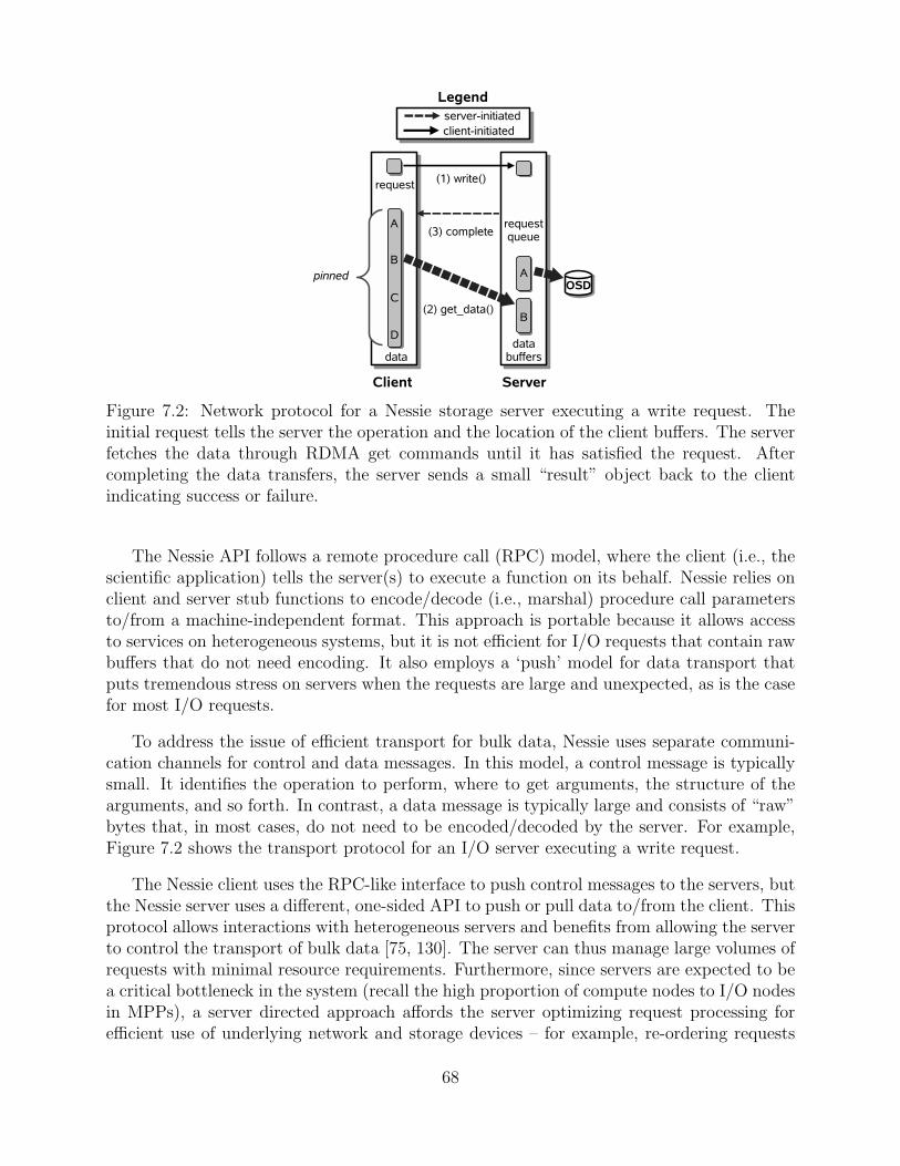
Figure 7.2: Network protocol for a Nessie storage server executing a write request. Theinitial request tells the server the operation and the location of the client buffers. The serverfetches the data through RDMA get commands until it has satisfied the request. Aftercompleting the data transfers, the server sends a small “result” object back to the clientindicating success or failure.

The Nessie API follows a remote procedure call (RPC) model, where the client (i.e., thescientific application) tells the server(s) to execute a function on its behalf. Nessie relies onclient and server stub functions to encode/decode (i.e., marshal) procedure call parametersto/from a machine-independent format. This approach is portable because it allows accessto services on heterogeneous systems, but it is not efficient for I/O requests that contain rawbuffers that do not need encoding. It also employs a ‘push’ model for data transport thatputs tremendous stress on servers when the requests are large and unexpected, as is the casefor most I/O requests.

To address the issue of efficient transport for bulk data, Nessie uses separate communi-cation channels for control and data messages. In this model, a control message is typicallysmall. It identifies the operation to perform, where to get arguments, the structure of thearguments, and so forth. In contrast, a data message is typically large and consists of “raw”bytes that, in most cases, do not need to be encoded/decoded by the server. For example,Figure 7.2 shows the transport protocol for an I/O server executing a write request.

The Nessie client uses the RPC-like interface to push control messages to the servers, butthe Nessie server uses a different, one-sided API to push or pull data to/from the client. Thisprotocol allows interactions with heterogeneous servers and benefits from allowing the serverto control the transport of bulk data [75, 130]. The server can thus manage large volumes ofrequests with minimal resource requirements. Furthermore, since servers are expected to bea critical bottleneck in the system (recall the high proportion of compute nodes to I/O nodesin MPPs), a server directed approach affords the server optimizing request processing forefficient use of underlying network and storage devices – for example, re-ordering requests

68

to a storage device [75].

7.3 A Simple Data-Transfer Service

The data-transfer service is included in the “examples/xfer-service/” directory of the Triospackage. This example demonstrates how to construct a simple client and server that transferan array of 16-byte data structures from a parallel application to a set of servers. The codeserves three purposes: it is the primary example for how to develop a data service, it is usedto test correctness of the Nessie APIs, and we use it to evaluate network performance of theNessie protocols.

Creating the transfer-service requires the following three steps:

1. Define the functions and their arguments.

2. Implement the client stubs.

3. Implement the server.

7.3.1 Defining the Service API

To properly evaluate the correctness of Nessie, we created procedures to transfer data to/froma remote server using both the control channel (through the function arguments or the resultstructure) and the data channel (using the RDMA put/get commands). We defined clientand server stubs for the following procedures:

xfer write encode Transfer an array of data structures to the server through the procedurearguments, forcing the client to encode the array before sending and the server todecode the array when receiving. We use this method to evaluate the performanceof the encoding/decoding the arguments. For large arrays, this method also tests ourtwo-phase transfer protocol in which the client pushes a small header of arguments andlets the server pull the remaining arguments on demand.

xfer write rdma Transfer an array of data structures to the server using the data channel.This procedure passes the length of the array in the arguments. The server then“pulls” the unencoded data from the client using the nssi get function. This methodevaluates the RDMA transfer performance for the nssi get data function.

xfer read encode Transfer an array of data structures to the client using the control chan-nel. This method tells the server to send the data array to the client through theresult data structure, forcing the server to encode the array before sending and theclient to decode the array when receiving. This procedure evaluates the performance

69

/∗ Data structure to transfer ∗/struct data t {

int int val; /∗ 4 bytes ∗/float float val; /∗ 4 bytes ∗/double double val; /∗ 8 bytes ∗/

};

/∗ Array of data structures ∗/typedef data t data array t<>;

/∗ Arguments for xfer write encode ∗/struct xfer write encode args {

data array t array;};

/∗ Arguments for xfer write rdma ∗/struct xfer write rdma args {

int len;};

...

Figure 7.3: Portion of the XDR file used for a data-transfer service.

of the encoding/decoding the arguments. For large arrays, this method also tests ourtwo-phase transfer protocol for the result structure in which the server pushes a smallheader of the result and lets the client pull the remaining result on demand (at thenssi wait function).

xfer read rdma Transfer an array of data structures to the client using the data channel.This procedure passes the length of the array in the arguments. The server then “puts”the unencoded data into the client memory using the nssi put data function. Thismethod evaluates the RDMA transfer performance for the nssi put data function.

Since the service needs to encode and decode remote procedure arguments, the service-developer has to define these data structures in an XDR file. Figure 7.3 shows a portion of theXDR file used for the data-transfer example. XDR data structures definitions are very similarto C data structure definitions. During build time, a macro called “TriosProcessXDR”converts the xdr file into a header and source file that call the XDR library to encode thedefined data structures. TriosProcessXDR executes the UNIX tool “rpcgen” the remoteprocedure call protocol compiler to generate the source and header files.

7.3.2 Implementing the client stubs

The client stubs provide the interface between the client application and the remote service.The stubs do nothing more than initialize the RPC arguments, and call the nssi call rpc

70

int xfer write rdma(const nssi service ∗svc,const data array t ∗arr,nssi request ∗req)

{xfer write rdma args args;int nbytes;

/∗ the only arg is size of array ∗/args.len = arr−>data array t len;

/∗ the RDMA buffer ∗/const data t ∗buf=array−>data array t val;

/∗ size of the RDMA buffer ∗/nbytes = args.len∗sizeof(data t);

/∗ call the remote methods ∗/nssi call rpc(svc, XFER WRITE RDMA OP,

&args, (char ∗)buf, nbytes,NULL, req);

}

Figure 7.4: Client stub for the xfer write rdma method of the transfer service.

method. For RDMA operations, the client also has to provide pointers to the appropriatedata buffers so the RDMA operations know where to put or get the data for the tranferoperation.

Figure 7.4 shows the client stub for the xfer write rdma method. Since the nssi call rpc

method is asynchronous. The client checks for completion of the operation by calling thenssi wait method with the nssi request as an argument.

7.3.3 Implementing the server

The server consists of some initialization code along with the server-side API stubs for anyexpected requests. Each server-side stub has the form described in Figure 7.5. The API in-cludes a request identifier, a peer identifier for the caller, decoded arguments for the method,and RDMA addresses for the data and result. The RDMA addresses allow the server stub towrite to or read from the memory on the client. In the case of the xfer write rdma srvr,the stub has to pull the data from the client using the data addr parameter and send aresult (success or failure) back to the client using the res addr parameter.

For complete details on how to create the transfer service code, refer to the online docu-mentation or the source code in the trios/examples directory.

71

int xfer write rdma srvr(const unsigned long request id,const NNTI peer t ∗caller,const xfer pull args ∗args,const NNTI buffer t ∗data addr,const NNTI buffer t ∗res addr)

{const int len = args−>len;int nbytes = len∗sizeof(data t);

/∗ allocate space for the buffer ∗/data t ∗buf = (data t ∗)malloc(nbytes);

/∗ fetch the data from the client ∗/nssi get data(caller,buf,nbytes,

data addr);

/∗ send the result to the client ∗/rc = nssi send result(caller,request id,

NSSI OK, NULL, res addr);

/∗ free buffer ∗/free(buf);

}

Figure 7.5: Server stub for the xfer write rdma method of the transfer service.

7.3.4 Performance of the transfer service

As mentioned earlier in the text, the transfer service is also a tool for evaluating the correct-ness and performance of the network protocols. Here we present performance results fromthree different HPC platforms: the Red Storm system at Sandia [30], a Cray XT3 that usesthe Seastar interconnect [26] interfaced through the Portals API [27]; RedSky, a cluster ofOracle/Sun Blade Servers on a an InfiniBand network; and the Cielo supercomputer, a CrayXE6 system that uses the new Gemini interconnect [6].

Figure 7.6 shows a comparison of using the xfer-write-rdma and xfer-write-encode

methods to transfer an array of data t data structures from Figure 7.3. The objective isto evaluate the overhead of the XDR encoding scheme. The xfer write rdma method hasvery little encoding overhead–just the cost of encoding the request. These results clearlydemonstrate the value of having separate control and data channels for bulk data, and whileit is possible to transfer all data through the control channel, it is clearly not an efficientway to implement a bulk data-transfer operation.

The Gemini port of Nessie, developed for the Cray XE6 Cielo system, is our latest portand still requires quite a bit of tuning to achieve reasonable performance. To demonstrate theefficiency of a well-tuned implementation, Figures 7.7(a) and 7.7(b) show xfer-write-rdma

72

● ● ● ● ● ● ● ● ●●

●

●

●

●

●

●

●

●●

●

●

● ● ●

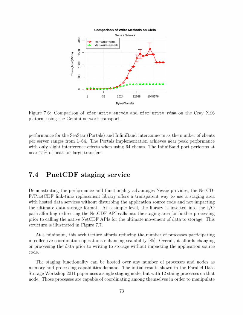
1 32 1024 32768 1048576

050

010

0015

0020

00

Comparison of Write Methods on Cielo

Bytes/Transfer

Thr

ough

put(

MiB

/s)

Gemini Network

● xfer−write−rdmaxfer−write−encode

Figure 7.6: Comparison of xfer-write-encode and xfer-write-rdma on the Cray XE6platorm using the Gemini network transport.

performance for the SeaStar (Portals) and InfiniBand interconnects as the number of clientsper server ranges from 1–64. The Portals implementation achieves near peak performancewith only slight interference effects when using 64 clients. The InfiniBand port performs atnear 75% of peak for large transfers.

7.4 PnetCDF staging service

Demonstrating the performance and functionality advantages Nessie provides, the NetCD-F/PnetCDF link-time replacement library offers a transparent way to use a staging areawith hosted data services without disturbing the application source code and not impactingthe ultimate data storage format. At a simple level, the library is inserted into the I/Opath affording redirecting the NetCDF API calls into the staging area for further processingprior to calling the native NetCDF APIs for the ultimate movement of data to storage. Thisstructure is illustrated in Figure 7.7.

At a minimum, this architecture affords reducing the number of processes participatingin collective coordination operations enhancing scalability [85]. Overall, it affords changingor processing the data prior to writing to storage without impacting the application sourcecode.

The staging functionality can be hosted over any number of processes and nodes asmemory and processing capabilities demand. The initial results shown in the Parallel DataStorage Workshop 2011 paper uses a single staging node, but with 12 staing processes on thatnode. Those processes are capable of coordinating among themselves in order to manipulate

73

● ● ● ● ● ● ● ● ●●

●

●

●

●

●

●

●

●●

● ● ● ● ●

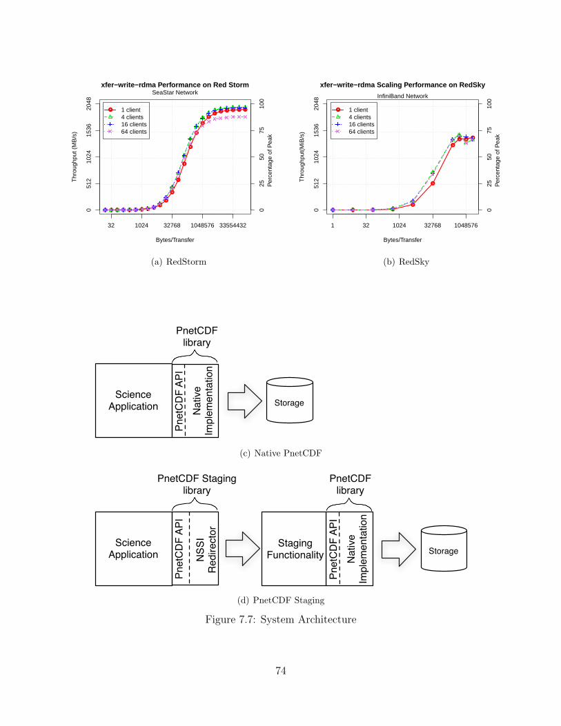
xfer−write−rdma Performance on Red Storm

Bytes/Transfer

Thr

ough

put (

MB

/s)

SeaStar Network

● 1 client4 clients16 clients64 clients

32 1024 32768 1048576 33554432

051

210

2415

3620

48

025

5075

100

Per

cent

age

of P

eak

(a) RedStorm

● ● ● ●

●

●

●

● ● ●

1 32 1024 32768 1048576

051

210

2415

3620

48

025

5075

100

Per

cent

age

of P

eak

xfer−write−rdma Scaling Performance on RedSky

Bytes/Transfer

Thr

ough

put(

MiB

/s)

InfiniBand Network

● 1 client4 clients16 clients64 clients

(b) RedSky

Science Application

PnetCDFlibrary

Pnet

CD

F AP

IN

ativ

eIm

plem

enta

tion

Storage

(c) Native PnetCDF

Science Application

PnetCDFlibrary

Pnet

CD

F AP

IN

ativ

eIm

plem

enta

tion

Storage

NSS

IR

edire

ctor

Pnet

CD

F AP

I

StagingFunctionality

PnetCDF Staginglibrary

(d) PnetCDF Staging

Figure 7.7: System Architecture

74

the data. Currently there are five data processing modes for the data staging area:

1. direct - immediately use the PnetCDF library to execute the request synchronouslywith the file system

2. caching independent - caches the write calls in the staging area until either no morebuffer space is available or the file close call is made. At that time, the data is writtenusing an independent IO mode rather than collective IO. This avoids both coordinationamong the staging processes and any additional data rearrangement prior to movementto storage.

3. aggregate independent - similar to caching independent except that the data is ag-gregated into larger, contiguous chunks as much as possible within all of the serverprocesses on a single compute node prior to writing to storage. That is, to optimizethe data rearrangement performance, the movement is restricted to stay within thesame node avoiding any network communication overhead.

4. caching collective - works like the chaching indpendent mode, except that it attemptsto use as many collective I/O calls as possible to write the data to storage. If the datapayloads are not evenly distributed across all of the staging processes, a number ofcollective calls corresponding to the number of smallest number of data payloads inany staging process followed by a series of independent calls to complete writing thedata.

5. aggregate collective - operates as a blend of the caching collective in that it tries to useas many collective I/O calls as possible to write the data, but uses the aggregationdata pre-processing steps to reduce the number of data packets written.

Unlike many aschronous staging approaches, the PnetCDF staging service ultimatelyperforms synchronously. The call to the file close function blocks until the data has beenflushed to storage.

Using the staging service at run time is a 4 step process. First, the staging area is launchedgenerating a list of contact strings. Each string contains the information necessary to reacha single staging process. The client (science application) can choose which client processcommunicates with which staging service process. Second, these strings are processed togenerate a standard XML-based format making client processing simpler and environmentvariables are set exposing the contact file filename in a standard way. Third, the scienceapplication is launched. Finally, as part of the PnetCDF initialization, the re-implementationof the PnetCDF reads the environment variable to determine the connection informationfile filename, reads the file, and broadcasts the connection information to all of the clientprocesses. These processes select one of the server processes with which to communicatebased on a load-balancing calculation.

The current functionality of increasing the performance of PnetCDF collective operationsis just a first step. The current architecture offer the ability to have any parallel or serial

75

processing engine installed in the staging area application. The scaling of this applicationis independent of scaling of the science application. This decoupling of concerns simplifiesprogramming of the integrated workflow of the simulation generating raw data and theanalysis routines distilling the data into the desired processed form.

Ultimately, this technique of reimplementing the API for accessing staging offers a wayto enhance the functionality of online scientific data processing without requiring changingthe application source code. As in the case of the PnetCDF service, these analysis or otherdata processing routines can be inserted as part of the I/O path with the data ultimatelyhitting the storage in the format prescribed by the original API.

7.4.1 PnetCDF staging service performance analysis

Evaluating the performance of the service is performed in two parts. First, an examination ofIOR [70] performance is evaluated followed by an I/O kernel for Sandia’s S3D [35] combustioncode.

7.4.1.1 IOR Performance

To evaluate the potential of PnetCDF staging, we measured the performance of our PnetCDFstaging library when used by the IOR benchmark code. IOR (Interleave-or-random) [70] isa highly configurable benchmark code from LLNL that IOR is often used to find the peakmeasurable throughput of an I/O system. In this case, IOR provides a tool for evaluatingthe impact of offloading the management overhead of the netCDF and PnetCDF librariesonto staging nodes.

Figure 7.8 shows measured throughput of three different experiments: writing a singleshared file using PnetCDF directly, writing a file-per-process using standard netCDF3, andwriting a single shared file using the PnetCDF staging service. In every experiment, eachclient wrote 25% of its compute-node memory, so we allocated one staging node for each fourcompute nodes to provide enough memory in the staging area to handle an I/O “dump”.

Results on Thunderbird show terrible performance for both the PnetCDF and netCDFfile-per-process case when using the library directly. The PnetCDF experiments maxed outat 217 MiB/s and reached the peak almost immediately. The PnetCDF shared file did notdo much better, achieving a peak throughput of 3.3 GiB/s after only 10s of clients. ThePnetCDF staging service, however, achieved an “effective” I/O rate of 28 GiB/s to a singleshared file. This is the rate observed by the application as the time to transfer the data fromthe application to the set of staging nodes. The staging nodes still have to write the data tostorage, but for applications with “bursty” IO patterns, staging is very effective.

76

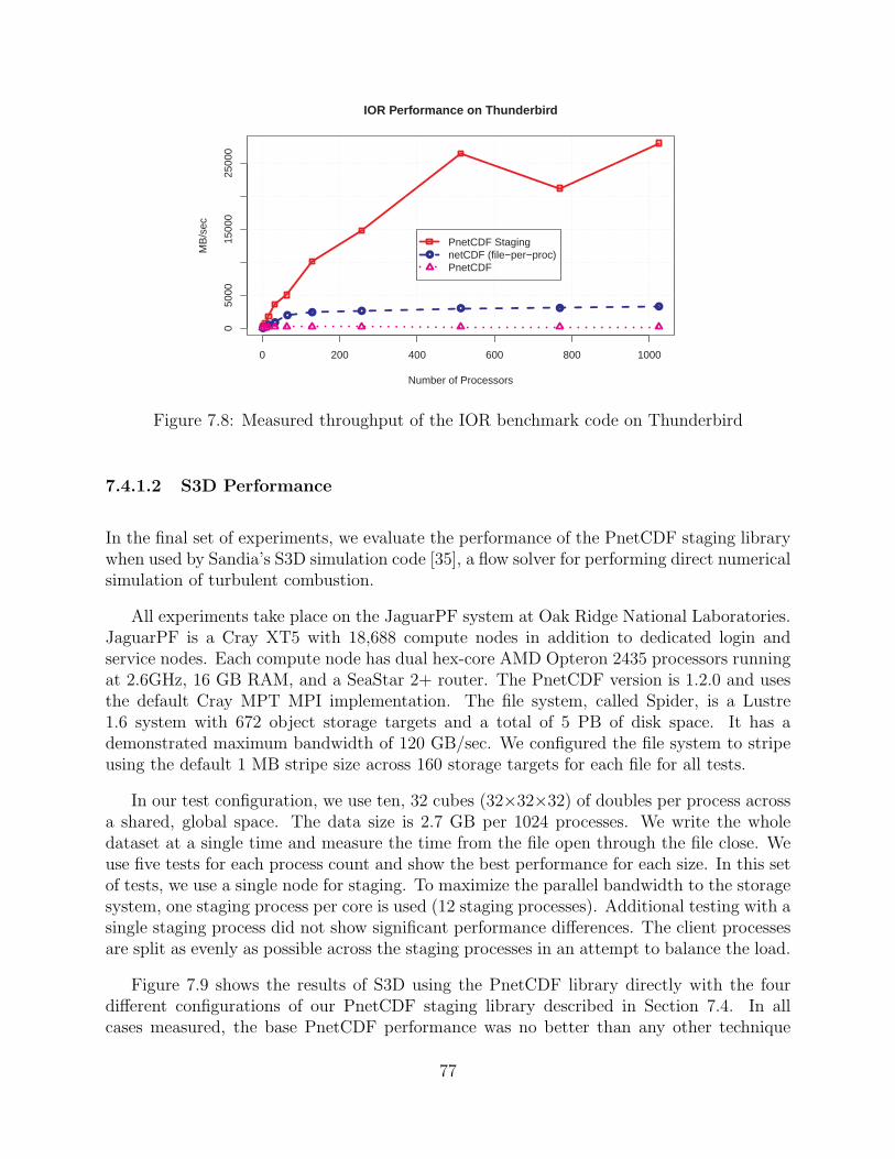
0 200 400 600 800 1000

050

0015

000

2500

0

IOR Performance on Thunderbird

Number of Processors

MB

/sec

●●●● ●● ● ● ● ● ●

●

PnetCDF StagingnetCDF (file−per−proc)PnetCDF

Figure 7.8: Measured throughput of the IOR benchmark code on Thunderbird

7.4.1.2 S3D Performance

In the final set of experiments, we evaluate the performance of the PnetCDF staging librarywhen used by Sandia’s S3D simulation code [35], a flow solver for performing direct numericalsimulation of turbulent combustion.

All experiments take place on the JaguarPF system at Oak Ridge National Laboratories.JaguarPF is a Cray XT5 with 18,688 compute nodes in addition to dedicated login andservice nodes. Each compute node has dual hex-core AMD Opteron 2435 processors runningat 2.6GHz, 16 GB RAM, and a SeaStar 2+ router. The PnetCDF version is 1.2.0 and usesthe default Cray MPT MPI implementation. The file system, called Spider, is a Lustre1.6 system with 672 object storage targets and a total of 5 PB of disk space. It has ademonstrated maximum bandwidth of 120 GB/sec. We configured the file system to stripeusing the default 1 MB stripe size across 160 storage targets for each file for all tests.

In our test configuration, we use ten, 32 cubes (32×32×32) of doubles per process acrossa shared, global space. The data size is 2.7 GB per 1024 processes. We write the wholedataset at a single time and measure the time from the file open through the file close. Weuse five tests for each process count and show the best performance for each size. In this setof tests, we use a single node for staging. To maximize the parallel bandwidth to the storagesystem, one staging process per core is used (12 staging processes). Additional testing with asingle staging process did not show significant performance differences. The client processesare split as evenly as possible across the staging processes in an attempt to balance the load.

Figure 7.9 shows the results of S3D using the PnetCDF library directly with the fourdifferent configurations of our PnetCDF staging library described in Section 7.4. In allcases measured, the base PnetCDF performance was no better than any other technique

77

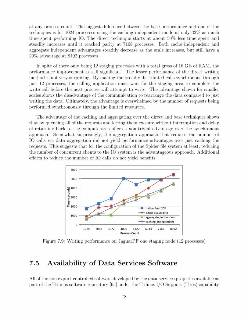
at any process count. The biggest difference between the base performance and one of thetechniques is for 1024 processes using the caching independent mode at only 32% as muchtime spent performing IO. The direct technique starts at about 50% less time spent andsteadily increases until it reached parity at 7168 processes. Both cache independent andaggregate independent advantages steadily decrease as the scale increases, but still have a20% advantage at 8192 processes.

In spite of there only being 12 staging processes with a total gross of 16 GB of RAM, theperformance improvement is still significant. The lesser performance of the direct writingmethod is not very surprising. By making the broadly distributed calls synchronous throughjust 12 processes, the calling application must wait for the staging area to complete thewrite call before the next process will attempt to write. The advantage shown for smallerscales shows the disadvantage of the communication to rearrange the data compared to justwriting the data. Ultimately, the advantage is overwhelmed by the number of requests beingperformed synchronously through the limited resources.

The advantage of the caching and aggregating over the direct and base techniques showsthat by queueing all of the requests and letting them execute without interruption and delayof returning back to the compute area offers a non-trivial advantage over the synchronousapproach. Somewhat surprisingly, the aggregation approach that reduces the number ofIO calls via data aggregation did not yield performance advantages over just caching therequests. This suggests that for the configuration of the Spider file system at least, reducingthe number of concurrent clients to the IO system is the advantageous approach. Additionalefforts to reduce the number of IO calls do not yield benefits.

0  

1000  

2000  

3000  

4000  

5000  

6000  

1024   2048   3072   4096   5120   6144   7168   8192  

Time  (secon

ds)  

Process  Count  

na.ve  PnetCDF  direct  via  staging  aggregate_indpendent  caching_independent  

Figure 7.9: Writing performance on JaguarPF one staging node (12 processes)

7.5 Availability of Data Services Software

All of the non export-controlled software developed by the data-services project is available aspart of the Trilinos software repository [65] under the Trilinos I/O Support (Trios) capability

78

area. Trios is a newly formed capability area to facilitate the co-design and development ofopen-source I/O tools and libraries developed for the ASC/CSSE program. Trilinos providesa fantastic development and testing environment and also provides a great tool for rapiddeployment of R&D codes into production applications.

7.6 Summary and Future Work

This chapter describes R&D at Sandia National Laboratories to use integrated data servicesto reduce the effective I/O cost for scientific applications. The Nessie framework providesan RPC abstraction that allows for the rapid development of experimental data services toexplore new new I/O techniques and programming models. We are using this framework toexplore improved access interfaces to staging areas, standard approaches integrate ‘in flight’data processing between the science application and storage, and we are exploring how toleverage the data services model with advanced accelerators such as GPGPUs and FPGAs.

While we expect data services to be common on next-generation systems, it is importantto note that data-services also provide practical solutions for applications in the currentgeneration of HPC systems. The results presented in this paper demonstrate the advantageof data-services on systems with three different interconnects: the Seastar for Cray XTsystems, the Gemini interconnect for Cray XE systems, and InfiniBand for large capacityclusters. In addition, we plan to modify the Exodus interface to use our PnetCDF stagingservice, providing an immediate impact to the Sierra applications, as well as any otherapplications using Sandia’s Exodus I/O library.

For next-generation systems, there are many improvements that could better supportdata services in a production environment. For example, runtime support for dynamic al-location and reconfiguration of nodes would allow for on-demand data-processing servicesthat effectively utilize system resources. Control over placement algorithms within an al-location would also allow data-services to better utilize networks to avoid contention withapplication communication and file-system communication. The projected promulgation ofNVRAM could also improve use of data-staging services, especially services primarily usedto manage large bursts of data. In short, nearly every proposed Exascale architecture wouldbenefit from, and perhaps require, a data-services architecture. Research prospects in thisarea will continue to grow throughout the next decade.

79

80

Chapter 8

In situ and In transit Visualizationand Analysis

Abstract: Traditional analysis workflow prescribes storing simulation results to disk andlater retrieving them to perform analysis and visualization for final results. This workflowbecomes increasingly difficult due to data movement at petascale and beyond. In situ [49]and In transit [98] are both techniques that by-pass the traditional workflow and managethe data movement problem. In situ refers to linking the visualization tools directly intothe simulation code to run in the same memory. In transit uses data staging, as describedin the previous chapter, and executes the analysis and visualization in a separate stagingjob concurrently with the main computation job. In the following chapter, we describeexperiments and results using these coupling techniques.

8.1 Background

Scientific simulation on parallel supercomputers is traditionally performed in four sequentialsteps: meshing, partitioning, solver, and visualization. Not all of these components areactually run on the supercomputer. In particular, the meshing and visualization usuallyhappen on smaller but more interactive computing resources. However, the previous decadehas seen a growth in both the need and ability to perform scalable parallel analysis, and thisgives motivation for coupling the solver and visualization.

The concept of running a visualization while the simulation is running is not new. It ismentioned in the 1987 National Science Foundation Visualization in Scientific Computingworkshop report [90], which is often attributed to launching the field of scientific visual-ization. It is only recently, however, as we move into petascale that the idea has startedgaining significant traction [2, 71]. Recent studies show that cost of specialized hardwardfor visualization at petascale is prohibitive [36] and that time spent writing data to andreading data from disk storage is beginning to dominate the time spent in both simulationand visualization [111, 112, 122].

There are a variety of analyses and visual representations available and appropriatenessof each depends highly on the type of problem being analyzed. Thus, it is important that

81

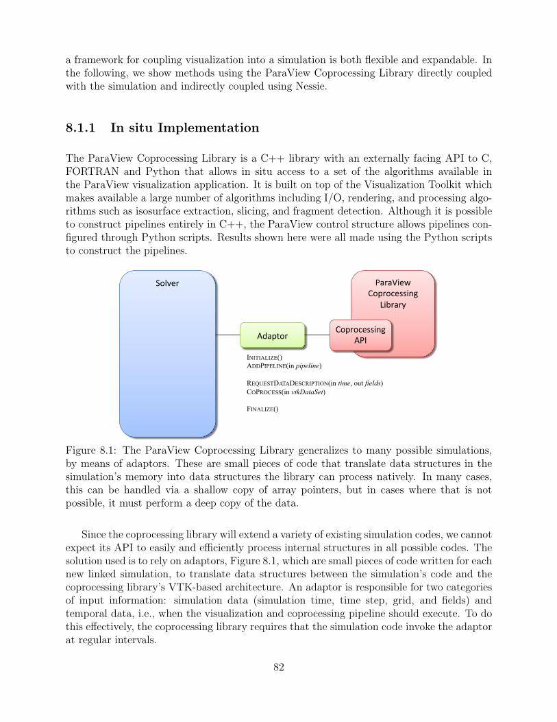
a framework for coupling visualization into a simulation is both flexible and expandable. Inthe following, we show methods using the ParaView Coprocessing Library directly coupledwith the simulation and indirectly coupled using Nessie.

8.1.1 In situ Implementation

The ParaView Coprocessing Library is a C++ library with an externally facing API to C,FORTRAN and Python that allows in situ access to a set of the algorithms available inthe ParaView visualization application. It is built on top of the Visualization Toolkit whichmakes available a large number of algorithms including I/O, rendering, and processing algo-rithms such as isosurface extraction, slicing, and fragment detection. Although it is possibleto construct pipelines entirely in C++, the ParaView control structure allows pipelines con-figured through Python scripts. Results shown here were all made using the Python scriptsto construct the pipelines.

Solver  ParaView Coprocessing 

Library 

Coprocessing API Adaptor 

INITIALIZE() ADDPIPELINE(in pipeline) REQUESTDATADESCRIPTION(in time, out fields) COPROCESS(in vtkDataSet) FINALIZE()

Figure 8.1: The ParaView Coprocessing Library generalizes to many possible simulations,by means of adaptors. These are small pieces of code that translate data structures in thesimulation’s memory into data structures the library can process natively. In many cases,this can be handled via a shallow copy of array pointers, but in cases where that is notpossible, it must perform a deep copy of the data.

Since the coprocessing library will extend a variety of existing simulation codes, we cannotexpect its API to easily and efficiently process internal structures in all possible codes. Thesolution used is to rely on adaptors, Figure 8.1, which are small pieces of code written for eachnew linked simulation, to translate data structures between the simulation’s code and thecoprocessing library’s VTK-based architecture. An adaptor is responsible for two categoriesof input information: simulation data (simulation time, time step, grid, and fields) andtemporal data, i.e., when the visualization and coprocessing pipeline should execute. To dothis effectively, the coprocessing library requires that the simulation code invoke the adaptorat regular intervals.

82

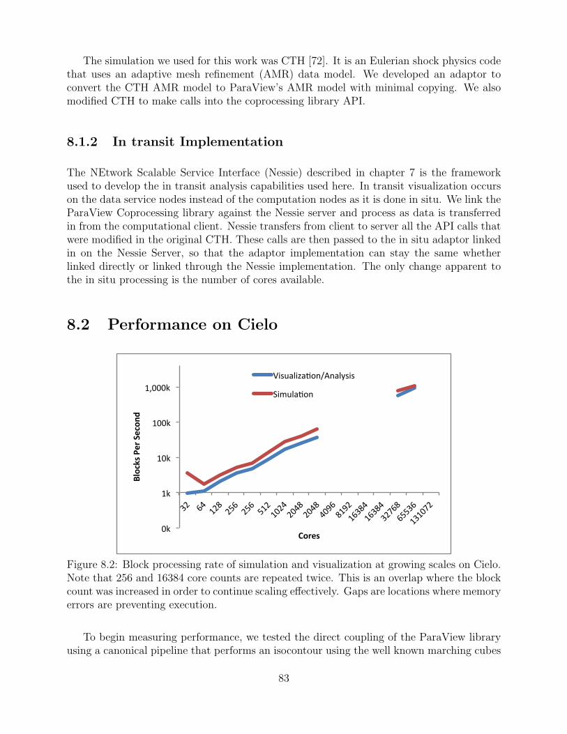
The simulation we used for this work was CTH [72]. It is an Eulerian shock physics codethat uses an adaptive mesh refinement (AMR) data model. We developed an adaptor toconvert the CTH AMR model to ParaView’s AMR model with minimal copying. We alsomodified CTH to make calls into the coprocessing library API.

8.1.2 In transit Implementation

The NEtwork Scalable Service Interface (Nessie) described in chapter 7 is the frameworkused to develop the in transit analysis capabilities used here. In transit visualization occurson the data service nodes instead of the computation nodes as it is done in situ. We link theParaView Coprocessing library against the Nessie server and process as data is transferredin from the computational client. Nessie transfers from client to server all the API calls thatwere modified in the original CTH. These calls are then passed to the in situ adaptor linkedin on the Nessie Server, so that the adaptor implementation can stay the same whetherlinked directly or linked through the Nessie implementation. The only change apparent tothe in situ processing is the number of cores available.

8.2 Performance on Cielo

0k  

1k  

10k  

100k  

1,000k  

32  

64  128  256  

256  

512  1024  2048  2048  4096  8192  

16384  

16384  

32768  

65536  

131072  

Blocks  Per  Secon

d  

Cores  

Visualiza5on/Analysis  

Simula5on  

Figure 8.2: Block processing rate of simulation and visualization at growing scales on Cielo.Note that 256 and 16384 core counts are repeated twice. This is an overlap where the blockcount was increased in order to continue scaling effectively. Gaps are locations where memoryerrors are preventing execution.

To begin measuring performance, we tested the direct coupling of the ParaView libraryusing a canonical pipeline that performs an isocontour using the well known marching cubes

83

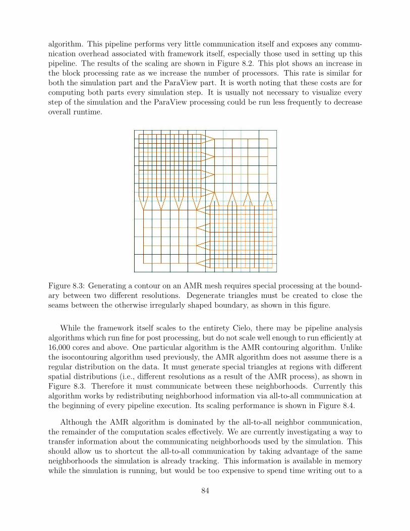
algorithm. This pipeline performs very little communication itself and exposes any commu-nication overhead associated with framework itself, especially those used in setting up thispipeline. The results of the scaling are shown in Figure 8.2. This plot shows an increase inthe block processing rate as we increase the number of processors. This rate is similar forboth the simulation part and the ParaView part. It is worth noting that these costs are forcomputing both parts every simulation step. It is usually not necessary to visualize everystep of the simulation and the ParaView processing could be run less frequently to decreaseoverall runtime.

Figure 8.3: Generating a contour on an AMR mesh requires special processing at the bound-ary between two different resolutions. Degenerate triangles must be created to close theseams between the otherwise irregularly shaped boundary, as shown in this figure.

While the framework itself scales to the entirety Cielo, there may be pipeline analysisalgorithms which run fine for post processing, but do not scale well enough to run efficiently at16,000 cores and above. One particular algorithm is the AMR contouring algorithm. Unlikethe isocontouring algorithm used previously, the AMR algorithm does not assume there is aregular distribution on the data. It must generate special triangles at regions with differentspatial distributions (i.e., different resolutions as a result of the AMR process), as shown inFigure 8.3. Therefore it must communicate between these neighborhoods. Currently thisalgorithm works by redistributing neighborhood information via all-to-all communication atthe beginning of every pipeline execution. Its scaling performance is shown in Figure 8.4.

Although the AMR algorithm is dominated by the all-to-all neighbor communication,the remainder of the computation scales effectively. We are currently investigating a way totransfer information about the communicating neighborhoods used by the simulation. Thisshould allow us to shortcut the all-to-all communication by taking advantage of the sameneighborhoods the simulation is already tracking. This information is available in memorywhile the simulation is running, but would be too expensive to spend time writing out to a

84

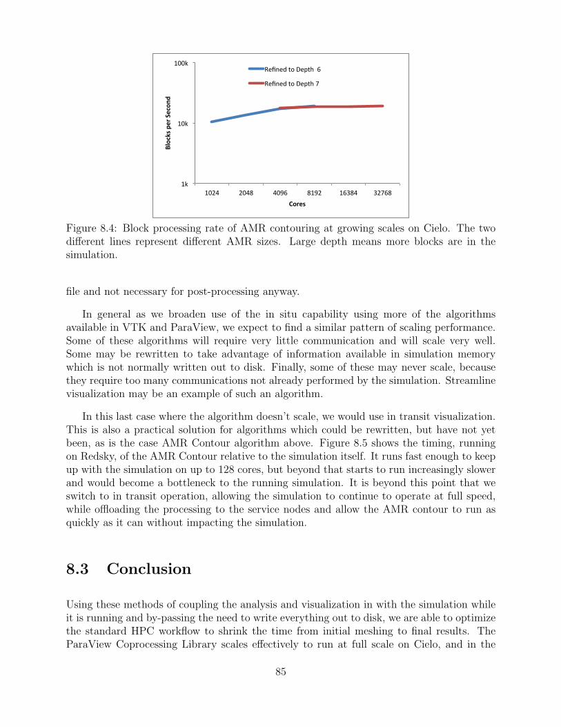
1k  

10k  

100k  

1024   2048   4096   8192   16384   32768  

Blocks  per  Secon

d  

Cores  

Refined  to  Depth    6  

Refined  to  Depth  7  

Figure 8.4: Block processing rate of AMR contouring at growing scales on Cielo. The twodifferent lines represent different AMR sizes. Large depth means more blocks are in thesimulation.

file and not necessary for post-processing anyway.

In general as we broaden use of the in situ capability using more of the algorithmsavailable in VTK and ParaView, we expect to find a similar pattern of scaling performance.Some of these algorithms will require very little communication and will scale very well.Some may be rewritten to take advantage of information available in simulation memorywhich is not normally written out to disk. Finally, some of these may never scale, becausethey require too many communications not already performed by the simulation. Streamlinevisualization may be an example of such an algorithm.

In this last case where the algorithm doesn’t scale, we would use in transit visualization.This is also a practical solution for algorithms which could be rewritten, but have not yetbeen, as is the case AMR Contour algorithm above. Figure 8.5 shows the timing, runningon Redsky, of the AMR Contour relative to the simulation itself. It runs fast enough to keepup with the simulation on up to 128 cores, but beyond that starts to run increasingly slowerand would become a bottleneck to the running simulation. It is beyond this point that weswitch to in transit operation, allowing the simulation to continue to operate at full speed,while offloading the processing to the service nodes and allow the AMR contour to run asquickly as it can without impacting the simulation.

8.3 Conclusion

Using these methods of coupling the analysis and visualization in with the simulation whileit is running and by-passing the need to write everything out to disk, we are able to optimizethe standard HPC workflow to shrink the time from initial meshing to final results. TheParaView Coprocessing Library scales effectively to run at full scale on Cielo, and in the

85

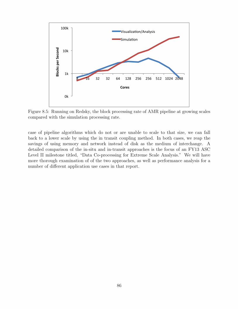
0k  

1k  

10k  

100k  

8   16   32   32   64   128   256   256   512   1024   2048  

Blocks  per  Secon

d  

Cores  

Visualiza2on/Analysis  

Simula2on  

Figure 8.5: Running on Redsky, the block processing rate of AMR pipeline at growing scalescompared with the simulation processing rate.

case of pipeline algorithms which do not or are unable to scale to that size, we can fallback to a lower scale by using the in transit coupling method. In both cases, we reap thesavings of using memory and network instead of disk as the medium of interchange. Adetailed comparison of the in-situ and in-transit approaches is the focus of an FY13 ASCLevel II milestone titled, “Data Co-processing for Extreme Scale Analysis.” We will havemore thorough examination of of the two approaches, as well as performance analysis for anumber of different application use cases in that report.

86

Chapter 9

Dynamic Shared Libraries on Cielo

Abstract: Popularity of dynamically linked executables continues to grow within the sci-entific computing community. The latest copy of a shared library can be accessed whenthe application is run. By contrast, statically linked applications use the version of the li-brary that was available when the application was built. Secondly, a shared library, as thename asserts, is shared across all application images running on a node. This can relievememory pressure, since the same text is accessed by all. Lastly, shared libraries are oftenmemory mapped from disk to further minimize the memory usage. Only the portions ofthe library that are being accessed need to reside in memory. Although attractive from aflexibility and resource reduction perspective, dynamically linked executables continue tosuffer performance issues on massively parallel processing (MPP) systems. This is particu-larly true for systems such as Cielo, where each node does not have a disk drive on whichto store the libraries. Instead, a custom file system configuration was installed on Cielo.This chapter describes the results of two experiments that analyze its performance. Resultsshowed it superior to the other available file systems. However, when the Charon applicationwas run in static and then dynamic link configurations, run time was increased by 34% on8192 cores. The chapter concludes with possible areas for further investigation, including apossible Linux kernel bug.

9.1 Motivation for the Implementation

Historically, applications running in capability mode are built (i.e. linked) statically. In-creasingly, application code groups are asking for the flexibility provided by dynamic sharedobjects. Dynamically linked executables have been supported on desktop system for decades.More recently, they have been successfully used on cluster computers of considerable scale(a few thousand cores). When specifying the Cielo system, the procurement team elected torequire support for dynamically linked executables on compute nodes. However, full scaletesting was done with static binaries.

Following the delivery of the system, the Cielo bring-up team began assessing the Cray(and other) options for providing support for dynamic libraries. We considered both hard-ware and software alternatives to achieve as much scalability as possible when using a dy-namically linked executable. One important aspect was that in addition to system shared

87

objects, the user community wished to provide their own shared libraries and other dynamicobjects, such as python modules.

As implied by the adjective, dynamic, requests for shared objects are asynchronous.Since they are unpredictable, they can introduce noise to a bulk synchronous application.Consistent quality of service for file access cannot be assured. Secondly, since all of Cielo’sjobs are SPMD (single program, multiple data), the I/O node serving the shared object filecan be flooded trying to satisfy a request from every single process in the job. With over100,000 cores, that could be a very large number of requests.

We elected to remain with the Linux software solution for linking and loading dynamicshared objects. This implementation is familiar to the Cielo user community and is supportedby all third party libraries. It is not trivial and a custom re-implementation was a largereffort/committment than we could make. On the down side, the Linux implementation is nottunable for parallel applications at all. We focused primarily on the hardware implementationto maximize parallel access to the shared objects.

9.2 Configuration and Implementation of the Solution

Cray proposed Cielo use Cray’s DVS (Data Virtualization Service) to distribute the system-provided shared libraries to compute nodes. DVS makes use of the read-only nature ofshared libraries to enable parallel access from compute nodes. Multiple DVS servers can beconfigured to serve some unique subset of compute nodes. The first compute node to askfor a shared library will ask its pre-defined DVS server. This DVS server will then ask forthe data from the single NFS server hosting the disk with the library/file. Any subsequentrequests to that pre-defined DVS server can hopefully be satisfied locally in its cache andthere won’t be a need to re-request from the NFS server. Other DVS servers, serving theremaining compute nodes, will need to go back to the NFS server. In this case, the NFSserver should have the file contents cached, eliminating the need to do the actual disk I/O.While caches are constrained by memory size, this design can significantly reduce the numberof accesses to the physical file. It distributes the requests between the DVS servers and theone NFS server.

There were several options for where to place user provided shared libraries. The optionsand their pros and cons are discussed fully in [73]. While no solution was ideal, we electedto mimic the solution used by Cray for system shared libraries that is described above. Thefile system serving the user-built shared libraries to the compute nodes is mounted read-only. It is served for read and write access from the login nodes where user compilations areperformed.

Figure 9.1 shows the before and after file system configuration. Changes are outlinedin red. To achieve scalability, 50 nodes were repurposed to serve the almost 9000 computenodes. This solution means that only 50 nodes are actually requesting the file data fromthe nodes serving the system and user shared objects. The hardware spreads out the I/O

88

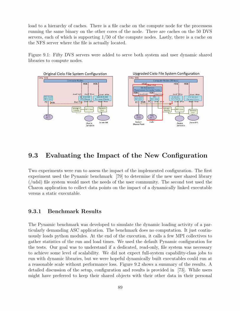
load to a hierarchy of caches. There is a file cache on the compute node for the processessrunning the same binary on the other cores of the node. There are caches on the 50 DVSservers, each of which is supporting 1/50 of the compute nodes. Lastly, there is a cache onthe NFS server where the file is actually located.

Figure 9.1: Fifty DVS servers were added to serve both system and user dynamic sharedlibraries to compute nodes.

9.3 Evaluating the Impact of the New Configuration

Two experiments were run to assess the impact of the implemented configuration. The firstexperiment used the Pynamic benchmark [79] to determine if the new user shared library(/udsl) file system would meet the needs of the user community. The second test used theCharon application to collect data points on the impact of a dynamically linked executableversus a static executable.

9.3.1 Benchmark Results

The Pynamic benchmark was developed to simulate the dynamic loading activity of a par-ticularly demanding ASC application. The benchmark does no computation. It just contin-uously loads python modules. At the end of the execution, it calls a few MPI collectives togather statistics of the run and load times. We used the default Pynamic configuration forthe tests. Our goal was to understand if a dedicated, read-only, file system was necessaryto achieve some level of scalability. We did not expect full-system capability-class jobs torun with dynamic libraries, but we were hopeful dynamically built executables could run ata reasonable scale without performance loss. Figure 9.2 shows a summary of the results. Adetailed discussion of the setup, configuration and results is provided in [73]. While usersmight have preferred to keep their shared objects with their other data in their personal

89

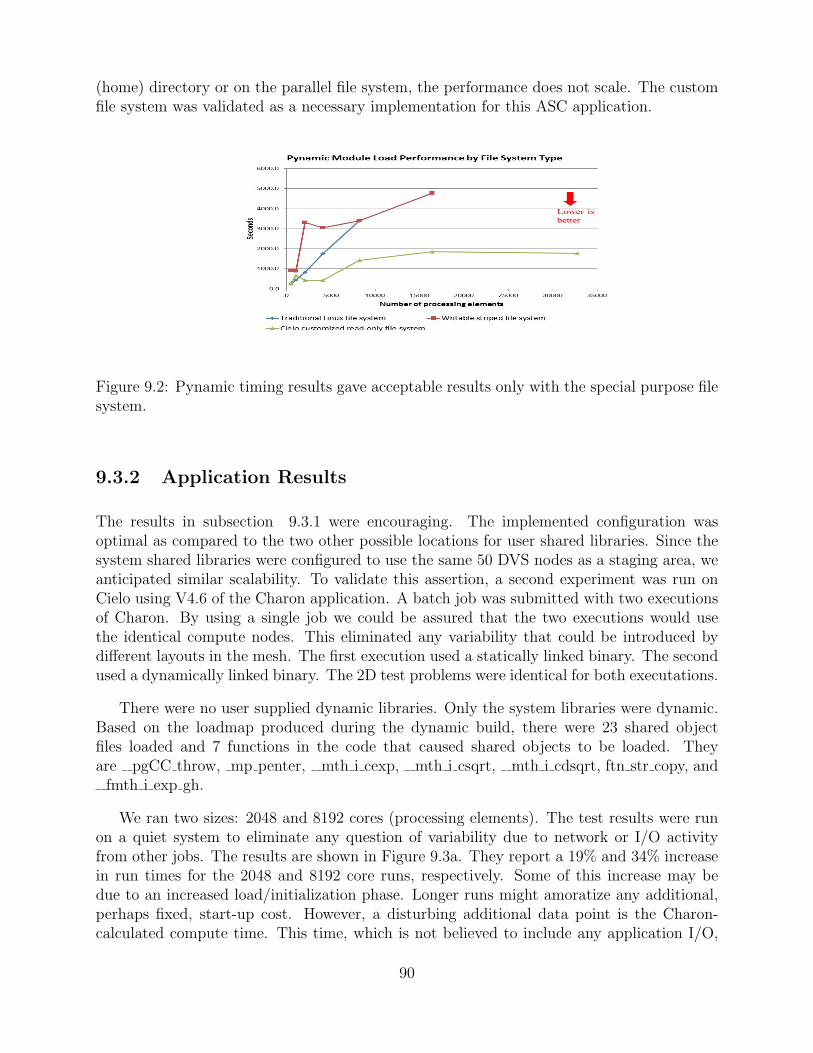
(home) directory or on the parallel file system, the performance does not scale. The customfile system was validated as a necessary implementation for this ASC application.

Figure 9.2: Pynamic timing results gave acceptable results only with the special purpose filesystem.

9.3.2 Application Results

The results in subsection 9.3.1 were encouraging. The implemented configuration wasoptimal as compared to the two other possible locations for user shared libraries. Since thesystem shared libraries were configured to use the same 50 DVS nodes as a staging area, weanticipated similar scalability. To validate this assertion, a second experiment was run onCielo using V4.6 of the Charon application. A batch job was submitted with two executionsof Charon. By using a single job we could be assured that the two executions would usethe identical compute nodes. This eliminated any variability that could be introduced bydifferent layouts in the mesh. The first execution used a statically linked binary. The secondused a dynamically linked binary. The 2D test problems were identical for both executations.

There were no user supplied dynamic libraries. Only the system libraries were dynamic.Based on the loadmap produced during the dynamic build, there were 23 shared objectfiles loaded and 7 functions in the code that caused shared objects to be loaded. Theyare pgCC throw, mp penter, mth i cexp, mth i csqrt, mth i cdsqrt, ftn str copy, andfmth i exp gh.

We ran two sizes: 2048 and 8192 cores (processing elements). The test results were runon a quiet system to eliminate any question of variability due to network or I/O activityfrom other jobs. The results are shown in Figure 9.3a. They report a 19% and 34% increasein run times for the 2048 and 8192 core runs, respectively. Some of this increase may bedue to an increased load/initialization phase. Longer runs might amoratize any additional,perhaps fixed, start-up cost. However, a disturbing additional data point is the Charon-calculated compute time. This time, which is not believed to include any application I/O,

90

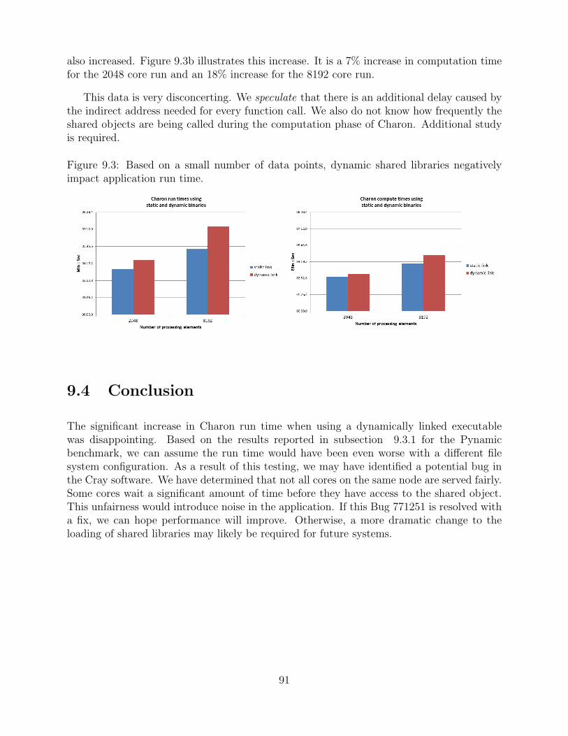
also increased. Figure 9.3b illustrates this increase. It is a 7% increase in computation timefor the 2048 core run and an 18% increase for the 8192 core run.

This data is very disconcerting. We speculate that there is an additional delay caused bythe indirect address needed for every function call. We also do not know how frequently theshared objects are being called during the computation phase of Charon. Additional studyis required.

Figure 9.3: Based on a small number of data points, dynamic shared libraries negativelyimpact application run time.

9.4 Conclusion

The significant increase in Charon run time when using a dynamically linked executablewas disappointing. Based on the results reported in subsection 9.3.1 for the Pynamicbenchmark, we can assume the run time would have been even worse with a different filesystem configuration. As a result of this testing, we may have identified a potential bug inthe Cray software. We have determined that not all cores on the same node are served fairly.Some cores wait a significant amount of time before they have access to the shared object.This unfairness would introduce noise in the application. If this Bug 771251 is resolved witha fix, we can hope performance will improve. Otherwise, a more dramatic change to theloading of shared libraries may likely be required for future systems.

91

92

Chapter 10

Process Replication for Reliability

Abstract: As high-end computing machines continue to grow in size, issues such as faulttolerance and reliability limit application scalability. Current techniques to ensure progressacross faults, like checkpoint-restart, are increasingly problematic at these scales due to ex-cessive overheads predicted to more than double an application’s time to solution. Replicatedcomputing techniques, particularly state machine replication, long used in distributed andmission critical systems, have been suggested as an alternative to checkpoint-restart. In thischapter, we evaluate the viability of using state machine replication as the primary faulttolerance mechanism for upcoming exascale systems. We use a combination of modeling,empirical analysis, and simulation to study the costs and benefits of this approach in com-parison to checkpoint/restart on a wide range of system parameters. These results, whichcover different failure distributions, hardware mean time between failures, and I/O band-widths, show that state machine replication is a potentially useful technique for meeting thefault tolerance demands of HPC applications on future exascale platforms.

10.1 Introduction

Process replication, generally referred to as state machine replication [126], is a well-knowntechnique for tolerating faults in systems that target high-availability. In this approach, aprocess’s state is replicated such that if the process fails, its replica is available or can begenerated to assume the original process’s role without disturbing the other application pro-cesses. Process replication can be costly in terms of space if replicas have dedicated resourcesor time if replicas are co-located with other primary processes. However, process replicationcan dramatically increase an application’s mean time to interrupt (MTTI). Additionally,variants of this technique can detect or correct faults that do not crash a process but insteadcause it to yield incorrect results [32].

Primarily due to its high costs, process replication has been examined only in a lim-ited manner for high performance computing (HPC) systems [132]. Instead, HPC appli-cations have relied primarily on rollback recovery techniques [46], particularly coordinatedcheckpoint/restart, where application state is periodically written to stable storage (check-pointed), and when failures occur, this state is used to recover the application to a previouslyknown-good state. However, future exascale systems are expected to present a much more

93

challenging fault tolerance environment to applications than current systems [17]. Addi-tionally, recent studies conclude that for these systems, high failure rates coupled with highcheckpoint/restart overheads will render current rollback-recovery approaches infeasible. Forexample, several independent studies have concluded that potential exascale systems couldspend more than 50% of their time reading and writing checkpoints [47, 102, 128].

In this chapter, we examine the viability of the process replication paradigm as a pri-mary exascale fault tolerance mechanism, with checkpoint/restart providing secondary faulttolerance when necessary. Our goal is to understand the advantages and limitations of thisapproach for extreme scale computing systems. We focus on exascale MPI applications: re-dundant copies of MPI processes provide failover capabilities, which allow these applicationsto transparently run through most errors without the need for rollback. Checkpoint/restartaugments our process replication scheme in cases where process replication is insufficient,for example, if all replicas of a process crash simultaneously or become inconsistent due tofaults corrupting the machine state.

To summarize, we present a study of redundant computing for exascale applications toaddress the scalability concerns of disk-oriented coordinated checkpoint/restart techniquesand the inability of checkpoint/restart methods to tolerate undetected hardware errors andnon-crash failures (Section 10.2). Our results show that redundant computing should beconsidered as a viable approach for exascale systems because:

• Even at system scales less than those projected for exascale systems, our model-basedanalysis shows that process replication’s hardware overheads are less than those oftraditional checkpoint/restart (Section 10.5);

• Based on a full implementation MPI process replication that has been evaluated onmore than 4000 nodes of a Cray XT-3/4 system, our empirical analysis shows thatprocess replication overheads are minimal for real HPC applications (Section 10.6);and,

• Additional simulation-based analysis that includes both software and hardware over-heads shows that process replication is a viable alternative to traditional checkpoint/restarton systems with more than 20,000 sockets (Section 10.7), depending on system check-point I/O bandwidth and per-socket mean time between failures (MTBF).

94

10.2 Background

10.2.1 Disk-based Coordinated Checkpoint/Restart

10.2.1.1 Current State of Practice

Disk-based coordinated checkpoint/restart has been the dominant fault tolerance mechanismin high performance computing systems for at least the last 30 years. In current largedistributed memory HPC systems, this approach generally works as follows:

1. Applications periodically quiesce all activity at a global synchronization point, forexample a barrier;

2. After synchronization, all nodes send some fraction of application and system state,generally comprising most of system memory, over the network to dedicated I/O nodes;

3. These I/O nodes store received checkpoint information data to stable storage, currentlyhard disk-based storage;

4. In the event of application crash, the stored checkpoint can be used to restart theapplication at a prior known-good state.

The dominance of coordinated checkpoint-restart as the primary HPC fault tolerancetechnique rests on a number of key assumptions that have thus far remained true:

1. Application state can be saved and restored much more quickly than a system’s meantime to interrupt (MTTI);

2. The hardware and upkeep (e.g. power) costs of supporting frequent checkpointing area modest portion (currently perhaps 10-20%) of the system’s overall cost; and

3. System faults that do not crash (fail-stop) the system are very rare.

Heroic work in both I/O systems and hardware error detection has largely kept these as-sumptions valid through the present day, allowing large parallel applications to scale to overa petaflop of sustained performance in the face of occasional fault-induced system crashes.

10.2.1.2 Scaling of Coordinated Disk-based Checkpoint/Restart

There are a number of excellent studies investigating the efficiency of disk-based check-point/restart for large scale systems, including past petascale systems [47, 107, 46] andupcoming exascale systems [128, 7, 17]. These projections invalidate essentially all of the

95

assumptions on which traditional checkpoint/restart depend. For example, these studies sug-gest exascale MTTIs ranging from 3-37 minutes, checkpoint times for low memory systemstaking up to five hours, and significant non-crash system failures, for example undetectedDRAM errors.

We begin by assuming a 15-minute checkpoint time, a modest improvement over theapproximate 20 minute checkpoint time that supercomputers both a decade ago (ASCIRed [89]) and today (BlueGene and Jaguar [31]) achieve. We also assume a one hour systemMTTI, again a generous assumption given recent studies. Daly’s model [39] estimates thatsuch a system should checkpoint once every 27 minutes and would achieve only 44% systemutilization. Scaling the I/O system to achieve a utilization greater than 80% would requirecheckpoint times of approximately one minute. Assuming that the I/O system supportingthat 15 minute checkpoint took only 10% of the system’s original budget and I/O throughputscaled up perfectly, a simple Amdahl’s law calculation shows that an I/O supporting suchcheckpoint speeds would comprise 63% of the total cost of the system!

Checkpoint-restart is also problematic when dealing with non-crash failures such as so-called “soft errors”. In particular, checkpoint-restart preserves the impact of failures thatcorrupt application state. Addressing this would require application developers to eitherrestart an application from scratch or analyze the contents of their checkpoints looking forone prior to when the fault that corrupted application state occurred.

10.2.2 State Machine Replication

Redundant computation, process replication, and state machine replication have long histo-ries and have been used extensively in both distributed [58, 34] and mission critical systems[91, 12, 109, 126] as a technique to improve fault tolerance. State machine replication, thefocus of this paper, maintains one or more replicas of each node and assumes every nodecomputes deterministically in response to a given external input, for example a message be-ing received. It then uses an ordering protocol to guarantee all replicas see the same inputsin the same order, and additional communication to detect and recover from failures.

State machine replication offers a different set of trade-offs compared to rollback recoverytechniques such as checkpoint/restart. In particular, it completely masks a large percentageof system faults, preventing them from causing application failures without the need for roll-back. Some forms of state machine replication can also be used to detect and recover from awider range of failures than checkpoint/restart, potentially including Byzantine failures [32].Unlike checkpoint/restart, however, state machine replication is not sufficient by itself torecover from all node crash failures; faults that crash all of a node’s replicas will cause acomputation to fail.

This approach has previously been dismissed in HPC as being too expensive for themeager benefits that are seen at present machine scale. For the reasons described abovein Section 10.2.1, however, several authors have recently suggested using this technique in

96

HPC systems [128, 140, 48]. In the remainder of this paper, we examine the suitability of aspecific type of state machine replication in HPC systems.

10.3 Replication for Message Passing HPC Applica-

tions

10.3.1 Overview

State machine replication is conceptually straightforward in message passing-oriented HPCapplications. In this approach, each replica is created on independent hardware for everyprocessor rank in the original application of which failure cannot easily be tolerated. Notethat we do not require all ranks to be replicated—in master/slave-style computations wherethe master can recover from the loss of slaves, only the master might be replicated.

The replication system then guarantees that every replica receives the same messages inthe same order and that a copy of each message from one rank is sent to each replica inthe destination rank. In addition, the replication system must detect replica failures, repairfailed nodes when possible, and restart failed nodes from active replicas. The replicationsystem may also periodically check that replicated ranks have the same state.

Checkpoint/restart recovery is still required in this approach for recovery from faults thatfail all replicas of a particular process rank. It is also used to recover from situations wherereplica state becomes inconsistent, for example due to silent (undetected) failures.

10.3.2 Costs and Benefits

This approach requires significantly increased computational resources—at least double thehardware for replicated ranks. In cases where only portions of an application must bereplicated, these requirements are potentially modest. For many HPC applications (e.g.traditional stencil calculations), however, this approach doubles the required hardware—2N nodes are required to fully replicate a job that would otherwise run (perhaps muchmore slowly) on N nodes. In addition, there are runtime overheads for maintaining replicaconsistency.

With these costs, however, come significant advantages:

• Dramatically increased system MTTI. This approach dramatically reduces thenumber of faults visible to applications. Specifically, the application only sees faultsthat crash (or otherwise fail) all replicas of a particular rank.

• Significantly reduced I/O requirements. Increased system MTTI reduces the

97

speed at which checkpoints must be written to storage to allow applications to effec-tively utilize the system. A smaller fraction of the system cost and power budget mustas a result be spent on the I/O system.

• Detection of “soft errors”. By comparing the state of multiple replicas (e.g. usingmemory checksums) prior to writing a checkpoint, replication can detect if applicationstate has been corrupted and trigger restart from a previous checkpoint.

• Increased system flexibility. The extra nodes used for redundant computationwhen running the largest jobs can be used for providing extra system capacity whenrunning multiple smaller jobs for which fault tolerance is less of a concern. A systemthat uses N nodes and an expensive I/O system to reach exascale can only run 10010PF jobs at a time, for example. A system that uses 2N nodes and a less expensiveI/O system to reach exascale, however, can potentially run 200 10PF jobs at a time.

10.4 Evaluating Replication in Exascale Systems

The advantages described in Section 10.3 provide a compelling reason to examine the vi-ability of state machine replication for extreme-scale HPC systems. Without quantifiableperformance benefits compared to other approaches, however, state machine replication willnot be viable for use in exascale systems. The remainder of this paper therefore examinesthe performance costs and benefits of state machine replication.

10.4.1 Comparison Approach

Our primary performance evaluation criteria is: at what node counts, if any, state machinereplication provides quantitative performance advantages over past approaches particularlyin terms of system utilization, after accounting for the overheads of state machine replication.If, for example, state machine replication achieves 46% utilization at a given system socketcount and another technique only achieves 40% system utilization, we regard state machinereplication as superior at that point.

We use traditional checkpoint/restart fault tolerance as the baseline technique againstwhich to compare because its performance characteristics are well-understood. We hopethat comparing against a well-understood baseline will facilitate future comparisons againstother proposed exascale fault tolerance techniques as their costs and benefits at scale aremore fully quantified. A brief qualitative comparison with several such techniques, however,is provided in [55].

98

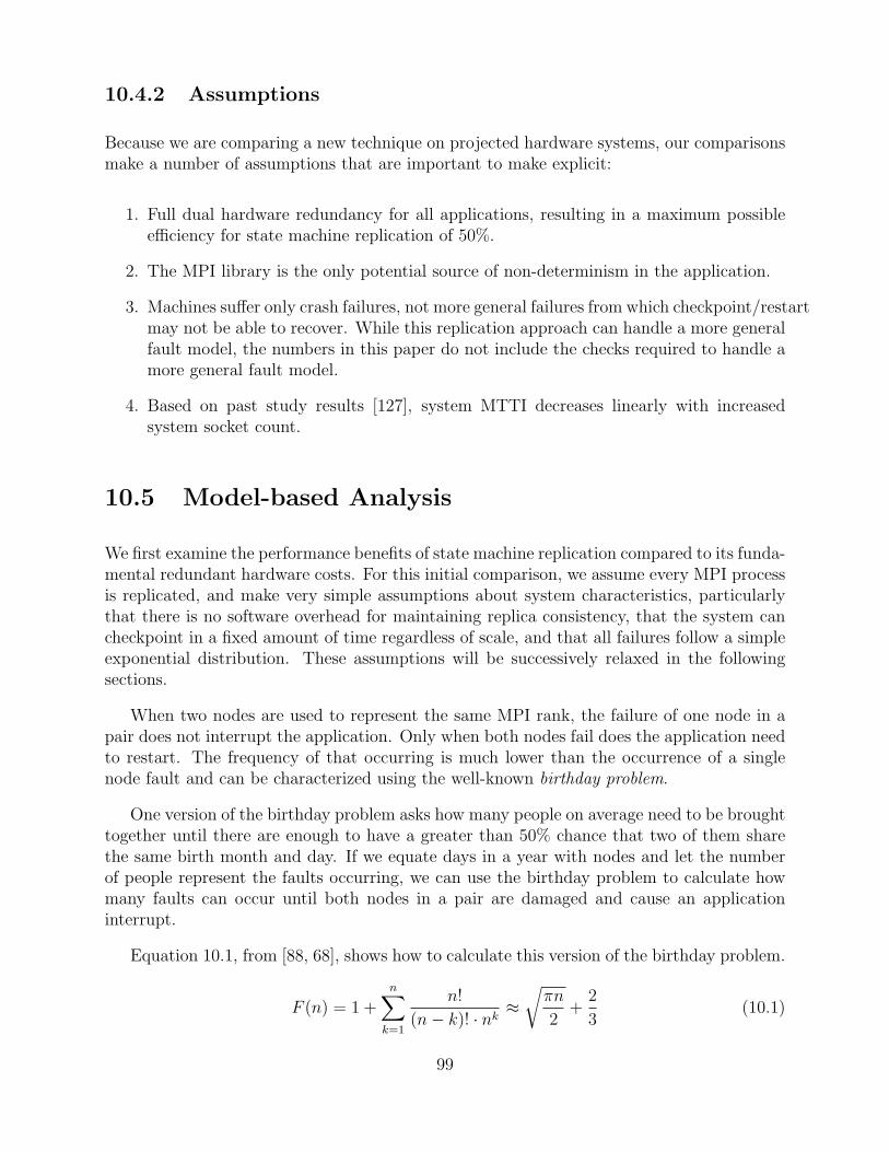
10.4.2 Assumptions

Because we are comparing a new technique on projected hardware systems, our comparisonsmake a number of assumptions that are important to make explicit:

1. Full dual hardware redundancy for all applications, resulting in a maximum possibleefficiency for state machine replication of 50%.

2. The MPI library is the only potential source of non-determinism in the application.

3. Machines suffer only crash failures, not more general failures from which checkpoint/restartmay not be able to recover. While this replication approach can handle a more generalfault model, the numbers in this paper do not include the checks required to handle amore general fault model.

4. Based on past study results [127], system MTTI decreases linearly with increasedsystem socket count.

10.5 Model-based Analysis

We first examine the performance benefits of state machine replication compared to its funda-mental redundant hardware costs. For this initial comparison, we assume every MPI processis replicated, and make very simple assumptions about system characteristics, particularlythat there is no software overhead for maintaining replica consistency, that the system cancheckpoint in a fixed amount of time regardless of scale, and that all failures follow a simpleexponential distribution. These assumptions will be successively relaxed in the followingsections.

When two nodes are used to represent the same MPI rank, the failure of one node in apair does not interrupt the application. Only when both nodes fail does the application needto restart. The frequency of that occurring is much lower than the occurrence of a singlenode fault and can be characterized using the well-known birthday problem.

One version of the birthday problem asks how many people on average need to be broughttogether until there are enough to have a greater than 50% chance that two of them sharethe same birth month and day. If we equate days in a year with nodes and let the numberof people represent the faults occurring, we can use the birthday problem to calculate howmany faults can occur until both nodes in a pair are damaged and cause an applicationinterrupt.

Equation 10.1, from [88, 68], shows how to calculate this version of the birthday problem.

F (n) = 1 +n∑

k=1

n!

(n − k)! · nk≈

√πn

2+

2

3(10.1)

99

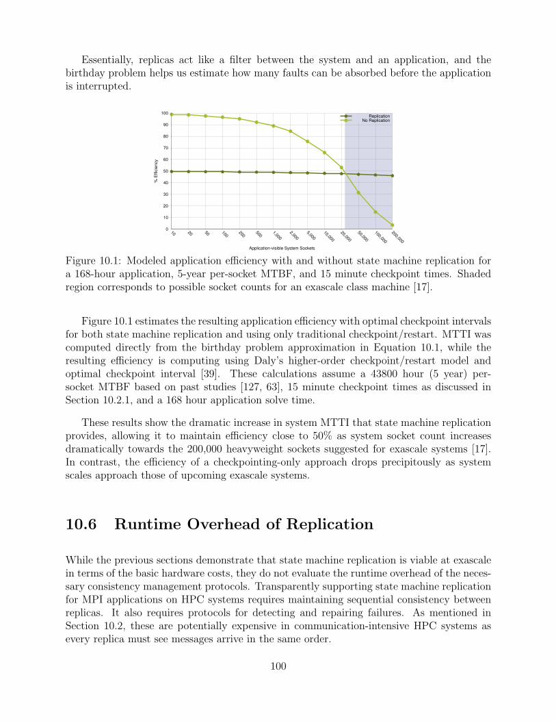
Essentially, replicas act like a filter between the system and an application, and thebirthday problem helps us estimate how many faults can be absorbed before the applicationis interrupted.

% E

ffic

ien

cy

Application-visible System Sockets

ReplicationNo Replication

0

10

20

30

40

50

60

70

80

90

100

10 20 50 100200

5001,000

2,000

5,000

10,000

20,000

50,000

100,000

200,000

Figure 10.1: Modeled application efficiency with and without state machine replication fora 168-hour application, 5-year per-socket MTBF, and 15 minute checkpoint times. Shadedregion corresponds to possible socket counts for an exascale class machine [17].

Figure 10.1 estimates the resulting application efficiency with optimal checkpoint intervalsfor both state machine replication and using only traditional checkpoint/restart. MTTI wascomputed directly from the birthday problem approximation in Equation 10.1, while theresulting efficiency is computing using Daly’s higher-order checkpoint/restart model andoptimal checkpoint interval [39]. These calculations assume a 43800 hour (5 year) per-socket MTBF based on past studies [127, 63], 15 minute checkpoint times as discussed inSection 10.2.1, and a 168 hour application solve time.

These results show the dramatic increase in system MTTI that state machine replicationprovides, allowing it to maintain efficiency close to 50% as system socket count increasesdramatically towards the 200,000 heavyweight sockets suggested for exascale systems [17].In contrast, the efficiency of a checkpointing-only approach drops precipitously as systemscales approach those of upcoming exascale systems.

10.6 Runtime Overhead of Replication

While the previous sections demonstrate that state machine replication is viable at exascalein terms of the basic hardware costs, they do not evaluate the runtime overhead of the neces-sary consistency management protocols. Transparently supporting state machine replicationfor MPI applications on HPC systems requires maintaining sequential consistency betweenreplicas. It also requires protocols for detecting and repairing failures. As mentioned inSection 10.2, these are potentially expensive in communication-intensive HPC systems asevery replica must see messages arrive in the same order.

100

(a) Mirror Protocol (b) Parallel Protocol

Figure 10.2: Basic replicated communication strategies for two different rMPI message con-sistency protocols. Additional protocol exchanges are needed in special cases such as MPI -

ANY SOURCE.

To study this overhead, we designed and implemented rMPI, a portable user-level MPIlibrary that provides redundant computation transparently to deterministic MPI applica-tions. rMPI is implemented on top of an existing MPI implementation using MPI profilinghooks. In the remainder of this section, we outline the basic design and implementation ofrMPI and measure the runtime overhead of this implementation for several real applicationson a large scale Cray XT-3/4 system. A complete description of rMPI, including low-levelprotocol and implementation details is available elsewhere [53, 22].

10.6.1 rMPI Design

The basic idea for the rMPI library is simple: replicate each MPI rank in an applicationand let the replicas continue when an original rank fails. To ensure consistent replica state,rMPI implements protocols that ensure identical message ordering between replicas. Unlikemore general state machine replication protocols [126, 32], these protocols are specific tothe needs of MPI in an attempt to reduce runtime overheads. In addition, rMPI uses theunderlying Reliability, Availability and Serviceability (RAS) system to detect node failures,and implements simple recovery protocols based on the consistency protocol used.

10.6.1.1 Basic Consistency Protocols

rMPI implements two different consistency protocols, named mirror and parallel , to ensurethat every replica receives a copy of every message and to order message reception at replicas.Both protocols take special care when dealing with MPI operations that could potentiallyresult in different message orders or MPI results being seen at different replicas. Note thatcollective operations in rMPI call the point-to-point operations internal to rMPI.

Figure 10.2(a) shows the basic organization of how the mirror protocol ensure that allreplicas see the same messages. In this figure, A and B represent distinct MPI ranks and A’and B’ are A’s and B’s replicas respectively. In this protocol, each sender transmits duplicate

101

messages to each of the destinations. Similarly, receivers must post multiple receives for theduplicate messages, but only require one of those messages to arrive in order to progress.This eases recovery after a failure, but doubles network bandwidth requirements.

The parallel protocol, in comparison, is shown in Figure 10.2(b). In this approach, eachreplica has a single corresponding replica for each other rank with which it communicates innon-failure scenarios. In the case of failure, one of the remaining replicas of a rank takes oversending and receiving for the failed node. This failure detection requires frequent message-based interaction with the reliability system on current systems. As a result, the parallelprotocol will initiate approximately double the number of messages for each send operation.These extra messages contain MPI envelope information and are small. Therefore, theparallel protocol reduces network bandwidth requirements for an increased number of shortmessages.

10.6.1.2 MPI Consistency Requirements

rMPI assumes that only MPI operations can result in non-deterministic behavior, and thereare a few specific MPI operations that can result in application-visible non-deterministicresults. For example, rMPI must address non-blocking operations, wildcard (e.g. MPI ANY -

SOURCE and MPI ANY TAG) receives, and operations such as MPI Wtime. As a first step, bothrMPI protocols use the notion of a leader node for each replicated MPI rank, while non-leader nodes are referred to as replicas or redundant nodes. When a leader drops out of acomputation, the protocol chooses a new replica from among those remaining for a rank totake over as leader. rMPI uses one high order bit in the tag to distinguish messages fromleader and replica nodes.

For the remainder of consistency protocol discussions, we focus on the mirror protocolimplementation; the parallel protocol implementation is generally similar and described inmore depth elsewhere [53]. For blocking non-wildcard receives, one of the the most commonforms of MPI communication, rMPI posts a receive for both senders A and A’ into the bufferprovided by the user. Since the data in the two arriving messages is identical, there is nodanger of corrupting the user buffer. If multiple messages from the replica set A arrive withthe same tag, rMPI must make sure that the first active and first redundant message arrivein the first buffer, and the second active and second redundant in the second buffer. rMPIachieves this by using one high-order tag bit, setting it on all outgoing redundant messagesand setting the same bit for all receives of redundant messages.

Due to MPI message-passing semantics and the possibility of wildcard source receives,this basic approach is not completely sufficient. To handle MPI ANY SOURCE and MPI ANY TAG,rMPI relies on explicit communication between the leader of each rank and other replicas.Essentially, rMPI allows only one actual wildcard receive to be posted at any time on anode, and then only on the leader. When a wildcard receive is matched, the leader thensends the MPI envelope information to replica nodes which then post for the actual messageneeded. The situation is more complicated for non-blocking wildcard receives, test, and wait

102

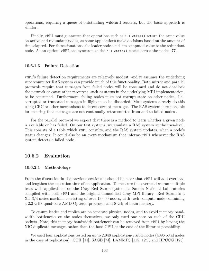
operations, requiring a queue of outstanding wildcard receives, but the basic approach issimilar.

Finally, rMPI must guarantee that operations such as MPI Wtime() return the same valueon active and redundant nodes, as some applications make decisions based on the amount oftime elapsed. For these situations, the leader node sends its computed value to the redundantnode. As an option, rMPI can synchronize the MPI Wtime() clocks across the nodes [77].

10.6.1.3 Failure Detection

rMPI’s failure detection requirements are relatively modest, and it assumes the underlyingsupercomputer RAS system can provide much of this functionality. Both mirror and parallelprotocols require that messages from failed nodes will be consumed and do not deadlockthe network or cause other resources, such as status in the underlying MPI implementation,to be consumed. Furthermore, failing nodes must not corrupt state on other nodes. I.e.,corrupted or truncated messages in flight must be discarded. Most systems already do thisusing CRC or other mechanisms to detect corrupt messages. The RAS system is responsiblefor ensuring that messages are not continually retransmitted from and to failed nodes .

For the parallel protocol we expect that there is a method to learn whether a given nodeis available or has failed. On our test systems, we emulate a RAS system at the user-level.This consists of a table which rMPI consults, and the RAS system updates, when a node’sstatus changes. It could also be an event mechanism that informs rMPI whenever the RASsystem detects a failed node.

10.6.2 Evaluation

10.6.2.1 Methodology

From the discussion in the previous sections it should be clear that rMPI will add overheadand lengthen the execution time of an application. To measure this overhead we ran multipletests with applications on the Cray Red Storm system at Sandia National Laboratoriescompiled with both rMPI and the original unmodified Cray MPI library. Red Storm is aXT-3/4 series machine consisting of over 13,000 nodes, with each compute node containinga 2.2 GHz quad-core AMD Opteron processor and 8 GB of main memory.

To ensure leader and replica are on separate physical nodes, and to avoid memory band-width bottlenecks on the nodes themselves, we only used one core on each of the CPUsockets. Note, this memory bandwidth bottleneck can be removed from rMPI by having theNIC duplicate messages rather than the host CPU at the cost of the libraries portability.

We used four applications tested on up to 2,048 application-visible nodes (4096 total nodesin the case of replication): CTH [44], SAGE [74], LAMMPS [115, 124], and HPCCG [125].

103

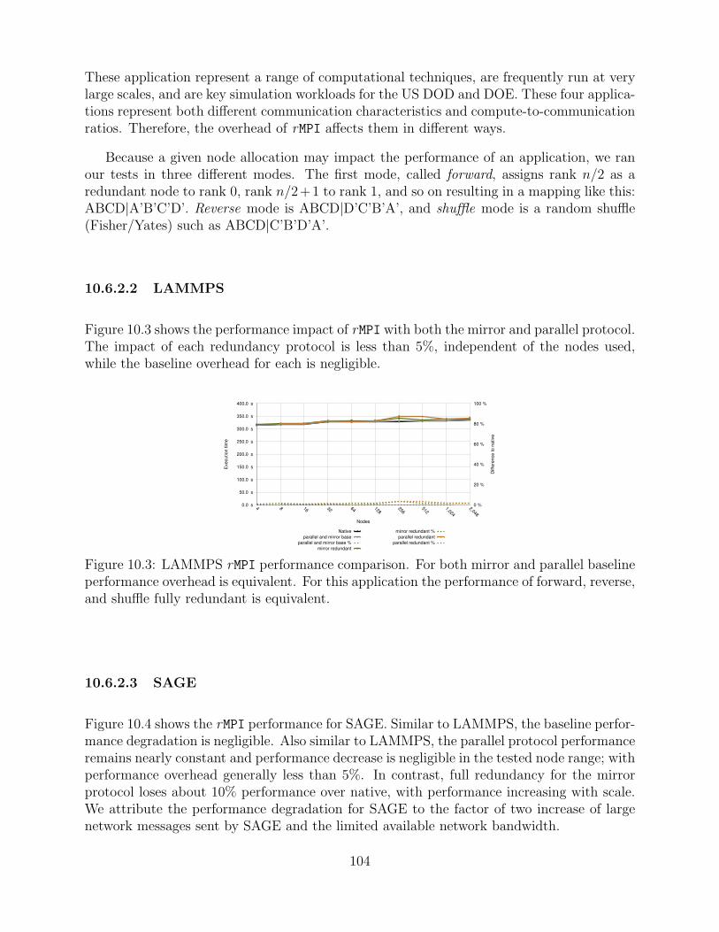
These application represent a range of computational techniques, are frequently run at verylarge scales, and are key simulation workloads for the US DOD and DOE. These four applica-tions represent both different communication characteristics and compute-to-communicationratios. Therefore, the overhead of rMPI affects them in different ways.

Because a given node allocation may impact the performance of an application, we ranour tests in three different modes. The first mode, called forward, assigns rank n/2 as aredundant node to rank 0, rank n/2+1 to rank 1, and so on resulting in a mapping like this:ABCD|A’B’C’D’. Reverse mode is ABCD|D’C’B’A’, and shuffle mode is a random shuffle(Fisher/Yates) such as ABCD|C’B’D’A’.

10.6.2.2 LAMMPS

Figure 10.3 shows the performance impact of rMPI with both the mirror and parallel protocol.The impact of each redundancy protocol is less than 5%, independent of the nodes used,while the baseline overhead for each is negligible.

Exe

cu

tio

n t

ime

Diffe

ren

ce

to

na

tive

Nodes

Native

parallel and mirror base

parallel and mirror base %

mirror redundant

mirror redundant %

parallel redundant

parallel redundant %

0.0 s

50.0 s

100.0 s

150.0 s

200.0 s

250.0 s

300.0 s

350.0 s

400.0 s

4 8 16 32 64 128256

5121,024

2,048

0 %

20 %

40 %

60 %

80 %

100 %

Figure 10.3: LAMMPS rMPI performance comparison. For both mirror and parallel baselineperformance overhead is equivalent. For this application the performance of forward, reverse,and shuffle fully redundant is equivalent.

10.6.2.3 SAGE

Figure 10.4 shows the rMPI performance for SAGE. Similar to LAMMPS, the baseline perfor-mance degradation is negligible. Also similar to LAMMPS, the parallel protocol performanceremains nearly constant and performance decrease is negligible in the tested node range; withperformance overhead generally less than 5%. In contrast, full redundancy for the mirrorprotocol loses about 10% performance over native, with performance increasing with scale.We attribute the performance degradation for SAGE to the factor of two increase of largenetwork messages sent by SAGE and the limited available network bandwidth.

104

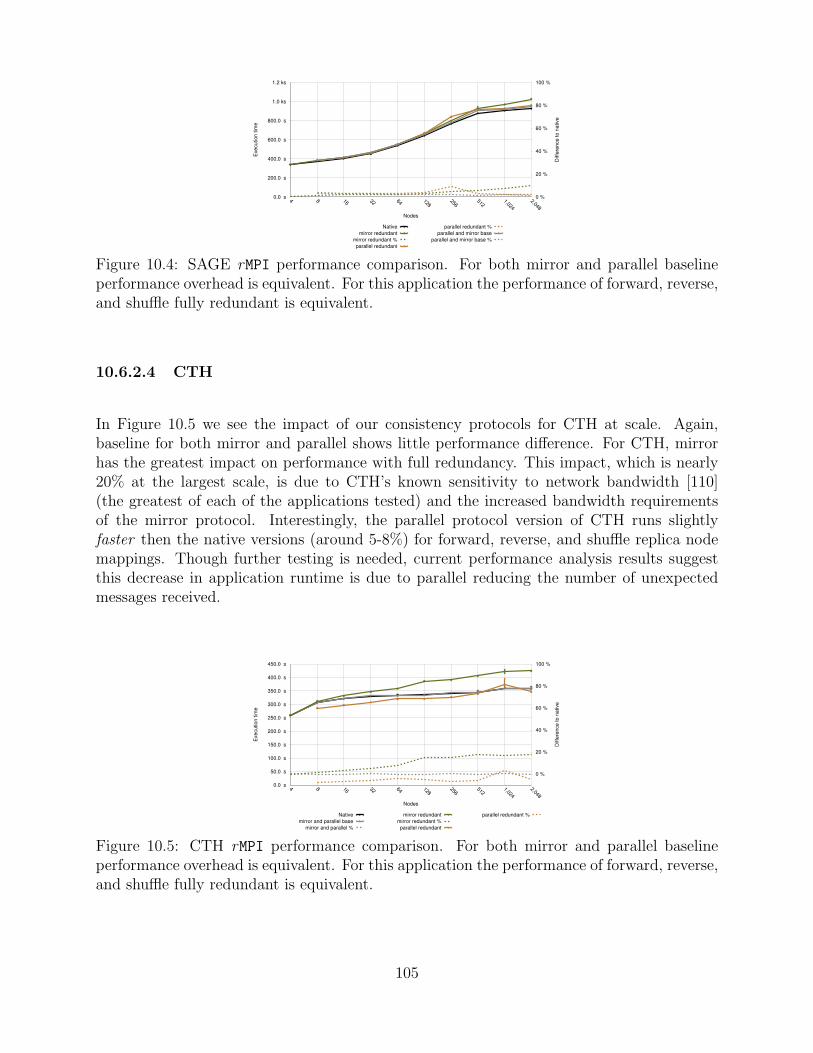
Exe

cu

tio

n t

ime

Diffe

ren

ce

to

na

tive

Nodes

Native

mirror redundant

mirror redundant %

parallel redundant

parallel redundant %

parallel and mirror base

parallel and mirror base %

0.0 s

200.0 s

400.0 s

600.0 s

800.0 s

1.0 ks

1.2 ks

4 8 16 32 64 128256

5121,024

2,048

0 %

20 %

40 %

60 %

80 %

100 %

Figure 10.4: SAGE rMPI performance comparison. For both mirror and parallel baselineperformance overhead is equivalent. For this application the performance of forward, reverse,and shuffle fully redundant is equivalent.

10.6.2.4 CTH

In Figure 10.5 we see the impact of our consistency protocols for CTH at scale. Again,baseline for both mirror and parallel shows little performance difference. For CTH, mirrorhas the greatest impact on performance with full redundancy. This impact, which is nearly20% at the largest scale, is due to CTH’s known sensitivity to network bandwidth [110](the greatest of each of the applications tested) and the increased bandwidth requirementsof the mirror protocol. Interestingly, the parallel protocol version of CTH runs slightlyfaster then the native versions (around 5-8%) for forward, reverse, and shuffle replica nodemappings. Though further testing is needed, current performance analysis results suggestthis decrease in application runtime is due to parallel reducing the number of unexpectedmessages received.

Exe

cu

tio

n t

ime

Diffe

ren

ce

to

na

tive

Nodes

Native

mirror and parallel base

mirror and parallel %

mirror redundant

mirror redundant %

parallel redundant

parallel redundant %

0.0 s

50.0 s

100.0 s

150.0 s

200.0 s

250.0 s

300.0 s

350.0 s

400.0 s

450.0 s

4 8 16 32 64 128256

5121,024

2,048

0 %

20 %

40 %

60 %

80 %

100 %

Figure 10.5: CTH rMPI performance comparison. For both mirror and parallel baselineperformance overhead is equivalent. For this application the performance of forward, reverse,and shuffle fully redundant is equivalent.

105

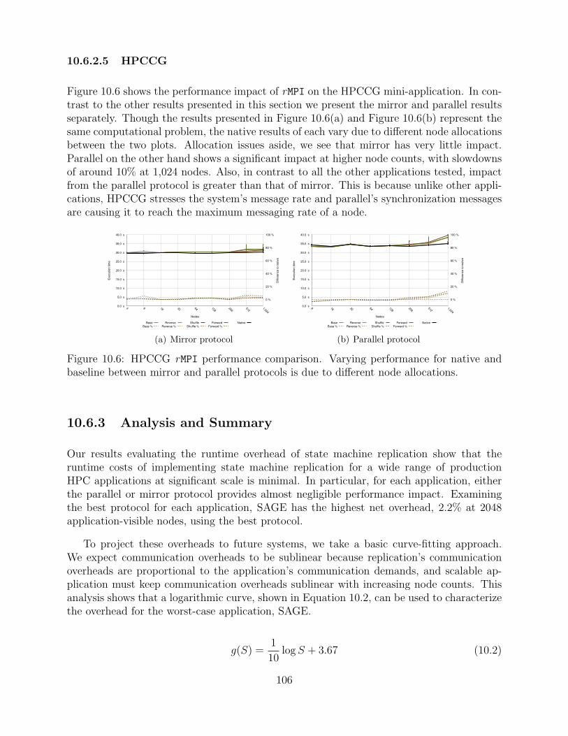
10.6.2.5 HPCCG

Figure 10.6 shows the performance impact of rMPI on the HPCCG mini-application. In con-trast to the other results presented in this section we present the mirror and parallel resultsseparately. Though the results presented in Figure 10.6(a) and Figure 10.6(b) represent thesame computational problem, the native results of each vary due to different node allocationsbetween the two plots. Allocation issues aside, we see that mirror has very little impact.Parallel on the other hand shows a significant impact at higher node counts, with slowdownsof around 10% at 1,024 nodes. Also, in contrast to all the other applications tested, impactfrom the parallel protocol is greater than that of mirror. This is because unlike other appli-cations, HPCCG stresses the system’s message rate and parallel’s synchronization messagesare causing it to reach the maximum messaging rate of a node.

Execution tim

e

Diffe

rence to n

ative

Nodes

Base

Base %

Reverse

Reverse %

Shuffle

Shuffle %

Forward

Forward %

Native

0.0 s

5.0 s

10.0 s

15.0 s

20.0 s

25.0 s

30.0 s

35.0 s

40.0 s

4 8 16 32 64 128256

5121,024

0 %

20 %

40 %

60 %

80 %

100 %

(a) Mirror protocol

Execution tim

e

Diffe

rence to n

ative

Nodes

Base

Base %

Reverse

Reverse %

Shuffle

Shuffle %

Forward

Forward %

Native

0.0 s

5.0 s

10.0 s

15.0 s

20.0 s

25.0 s

30.0 s

35.0 s

40.0 s

8 16 32 64 128256

5121,024

0 %

20 %

40 %

60 %

80 %

100 %

(b) Parallel protocol

Figure 10.6: HPCCG rMPI performance comparison. Varying performance for native andbaseline between mirror and parallel protocols is due to different node allocations.

10.6.3 Analysis and Summary

Our results evaluating the runtime overhead of state machine replication show that theruntime costs of implementing state machine replication for a wide range of productionHPC applications at significant scale is minimal. In particular, for each application, eitherthe parallel or mirror protocol provides almost negligible performance impact. Examiningthe best protocol for each application, SAGE has the highest net overhead, 2.2% at 2048application-visible nodes, using the best protocol.

To project these overheads to future systems, we take a basic curve-fitting approach.We expect communication overheads to be sublinear because replication’s communicationoverheads are proportional to the application’s communication demands, and scalable ap-plication must keep communication overheads sublinear with increasing node counts. Thisanalysis shows that a logarithmic curve, shown in Equation 10.2, can be used to characterizethe overhead for the worst-case application, SAGE.

g(S) =1

10log S + 3.67 (10.2)

106

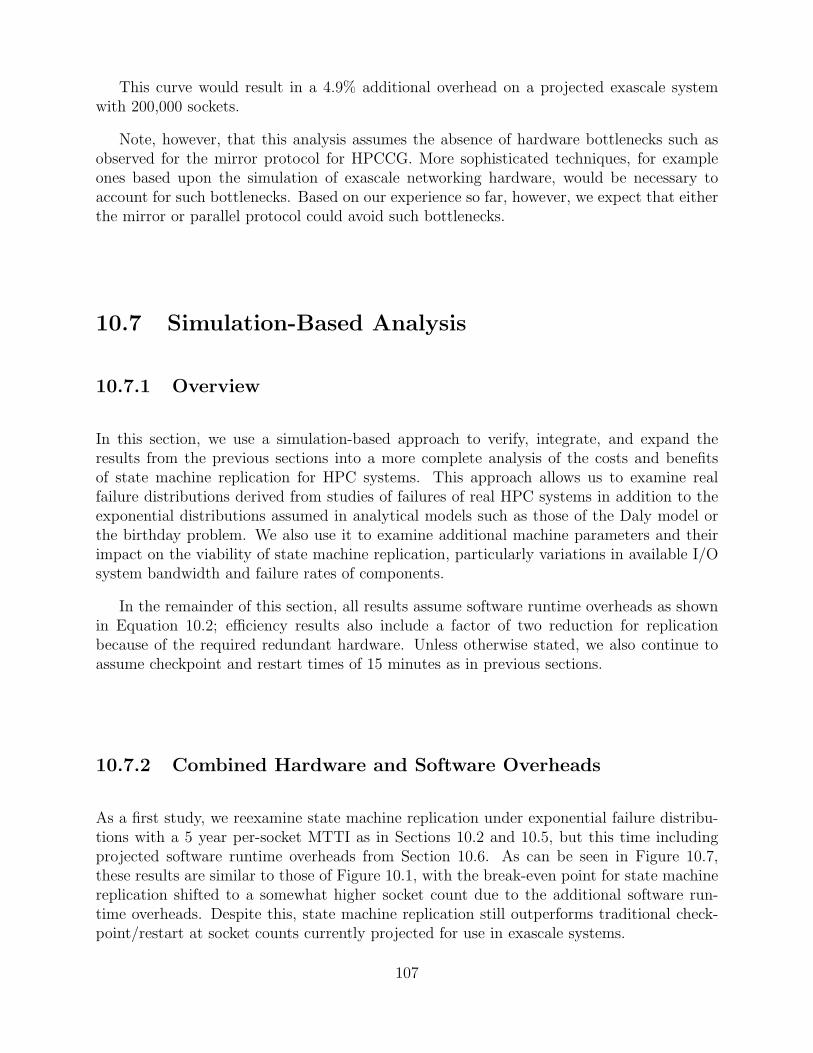
This curve would result in a 4.9% additional overhead on a projected exascale systemwith 200,000 sockets.

Note, however, that this analysis assumes the absence of hardware bottlenecks such asobserved for the mirror protocol for HPCCG. More sophisticated techniques, for exampleones based upon the simulation of exascale networking hardware, would be necessary toaccount for such bottlenecks. Based on our experience so far, however, we expect that eitherthe mirror or parallel protocol could avoid such bottlenecks.

10.7 Simulation-Based Analysis

10.7.1 Overview

In this section, we use a simulation-based approach to verify, integrate, and expand theresults from the previous sections into a more complete analysis of the costs and benefitsof state machine replication for HPC systems. This approach allows us to examine realfailure distributions derived from studies of failures of real HPC systems in addition to theexponential distributions assumed in analytical models such as those of the Daly model orthe birthday problem. We also use it to examine additional machine parameters and theirimpact on the viability of state machine replication, particularly variations in available I/Osystem bandwidth and failure rates of components.

In the remainder of this section, all results assume software runtime overheads as shownin Equation 10.2; efficiency results also include a factor of two reduction for replicationbecause of the required redundant hardware. Unless otherwise stated, we also continue toassume checkpoint and restart times of 15 minutes as in previous sections.

10.7.2 Combined Hardware and Software Overheads

As a first study, we reexamine state machine replication under exponential failure distribu-tions with a 5 year per-socket MTTI as in Sections 10.2 and 10.5, but this time includingprojected software runtime overheads from Section 10.6. As can be seen in Figure 10.7,these results are similar to those of Figure 10.1, with the break-even point for state machinereplication shifted to a somewhat higher socket count due to the additional software run-time overheads. Despite this, state machine replication still outperforms traditional check-point/restart at socket counts currently projected for use in exascale systems.

107

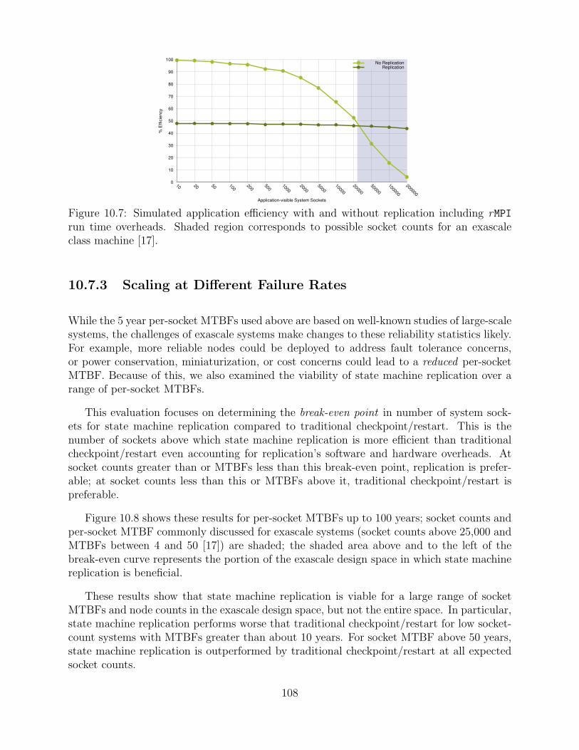
% E

ffic

ien

cy

Application-visible System Sockets

No ReplicationReplication

0

10

20

30

40

50

60

70

80

90

100

10 20 50 100200

5001000

20005000

10000

20000

50000

100000

200000

Figure 10.7: Simulated application efficiency with and without replication including rMPIrun time overheads. Shaded region corresponds to possible socket counts for an exascaleclass machine [17].

10.7.3 Scaling at Different Failure Rates

While the 5 year per-socket MTBFs used above are based on well-known studies of large-scalesystems, the challenges of exascale systems make changes to these reliability statistics likely.For example, more reliable nodes could be deployed to address fault tolerance concerns,or power conservation, miniaturization, or cost concerns could lead to a reduced per-socketMTBF. Because of this, we also examined the viability of state machine replication over arange of per-socket MTBFs.

This evaluation focuses on determining the break-even point in number of system sock-ets for state machine replication compared to traditional checkpoint/restart. This is thenumber of sockets above which state machine replication is more efficient than traditionalcheckpoint/restart even accounting for replication’s software and hardware overheads. Atsocket counts greater than or MTBFs less than this break-even point, replication is prefer-able; at socket counts less than this or MTBFs above it, traditional checkpoint/restart ispreferable.

Figure 10.8 shows these results for per-socket MTBFs up to 100 years; socket counts andper-socket MTBF commonly discussed for exascale systems (socket counts above 25,000 andMTBFs between 4 and 50 [17]) are shaded; the shaded area above and to the left of thebreak-even curve represents the portion of the exascale design space in which state machinereplication is beneficial.

These results show that state machine replication is viable for a large range of socketMTBFs and node counts in the exascale design space, but not the entire space. In particular,state machine replication performs worse that traditional checkpoint/restart for low socket-count systems with MTBFs greater than about 10 years. For socket MTBF above 50 years,state machine replication is outperformed by traditional checkpoint/restart at all expectedsocket counts.

108

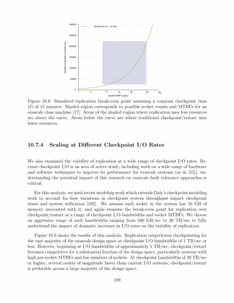
Num

ber

of S

ockets

for

bre

ak e

ven

Socket MTBF (years)

Break Even (δ = 15 min)

0

50000

100000

150000

200000

250000

300000

1 2 5 10 25 50 100

Figure 10.8: Simulated replication break-even point assuming a constant checkpoint time(δ) of 15 minutes. Shaded region corresponds to possible socket counts and MTBFs for anexascale class machine [17]. Areas of the shaded region where replication uses less resourcesare above the curve. Areas below the curve are where traditional checkpoint/restart useslower resources.

10.7.4 Scaling at Different Checkpoint I/O Rates

We also examined the viability of replication at a wide range of checkpoint I/O rates. Be-cause checkpoint I/O is an area of active study, including work on a wide range of hardwareand software techniques to improve its performance for exascale systems (as in [55]), un-derstanding the potential impact of this research on exascale fault tolerance approaches iscritical.

For this analysis, we used recent modeling work which extends Daly’s checkpoint modelingwork to account for how variations in checkpoint system throughput impact checkpointtimes and system utilization [102]. We assume each socket in the system has 16 GB ofmemory associated with it, and again examine the break-even point for replication overcheckpoint/restart at a range of checkpoint I/O bandwidths and socket MTBFs. We choosean aggressive range of such bandwidths ranging from 500 GB/sec to 30 TB/sec to fullyunderstand the impact of dramatic increases in I/O rates on the viability of replication.

Figure 10.9 shows the results of this analysis. Replication outperforms checkpointing forthe vast majority of the exascale design space at checkpoint I/O bandwidths of 1 TB/sec orless. However, beginning at I/O bandwidths of approximately 5 TB/sec, checkpoint/restartbecomes competitive for a substantial fraction of the design space, particularly systems withhigh per-socket MTBFs and low numbers of sockets. At checkpoint bandwidths of 30 TB/secor higher, several orders of magnitude faster than current I/O systems, checkpoint/restartis preferable across a large majority of the design space.

109

Num

ber

of S

ockets

for

bre

ak e

ven

Socket MTBF (years)

500GB/s1TB/s5TB/s

10TB/s30TB/s

0

50000

100000

150000

200000

250000

300000

1 2 5 10 25 50 100

Figure 10.9: “Break even” points for replication for various checkpoint bandwidth rates. Theshaded region corresponds to possible socket counts and socket MTBFs for exascale class ma-chines [17]. State machine replication is a viable approach for most checkpoint bandwidths,but with a checkpoint bandwidth greater than 30TB/sec, replication is inappropriate for themajority of the exascale design space. Areas of the shaded region where replication uses lessresources are above the curve. Areas below the curve are where traditional checkpoint/restartuses lower resources.

10.7.5 Non-Exponential Failure Distributions

Finally, we also examine the viability of replication with more realistic failure distributions.For failure information, we use numbers from a recent study of failures on two BlueGenesupercomputer systems, a 16,384 node system at Rennesseler Polytechnic Institute (RPI)and a 4,096 node system at Ecole Polytechnique Federale de Lausanne (EPFL) [63].

This study shows that failures in these systems are best described by a Weibull distri-bution with MTBFs of 6.6 hours (11.7 years/socket) and 8.4 hours (3.9 years/socket), andshape (β) values of 0.156 and 0.469, respectively. These β values (β < 1.0) describe distri-butions that decrease in probability over time; in HPC systems, this indicates that failuresare more likely to happen at the start of a system’s lifetime or an application run and reducein frequency as the system runs.

To examine the impact of these failure distributions, we build on the results of theprevious subsection and examine how the efficiency of replication and checkpoint/restartchange under Weibull failures assuming a fixed 1 TB/sec checkpoint bandwidth and 16 GBof memory per socket. Note that the systems from which these distributions were measuredexperienced a significant number of I/O system failures, and it is unclear how these failuresshould be properly scaled up to larger systems. As a result, we use the failure data fromthe larger of the two systems (the RPI system), and focus on how Weibull distributionschange the efficiency of replication and checkpoint/restart approach as opposed to the specific

110

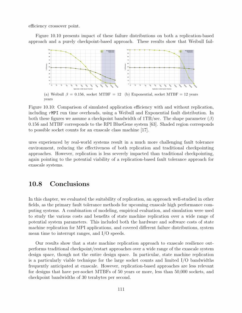
efficiency crossover point.

Figure 10.10 presents impact of these failure distributions on both a replication-basedapproach and a purely checkpoint-based approach. These results show that Weibull fail-

% E

ffic

iency

Application-visible System Sockets

No ReplicationReplication

0

10

20

30

40

50

60

70

80

90

100

10 20 50 100200

5001000

20005000

10000

20000

50000

100000

200000

(a) Weibull β = 0.156, socket MTBF = 12years

% E

ffic

iency

Application-visible System Sockets

No ReplicationReplication

0

10

20

30

40

50

60

70

80

90

100

10 20 50 100200

5001000

20005000

10000

20000

50000

100000

200000

(b) Exponential, socket MTBF = 12 years

Figure 10.10: Comparison of simulated application efficiency with and without replication,including rMPI run time overheads, using a Weibull and Exponential fault distribution. Inboth these figures we assume a checkpoint bandwidth of 1TB/sec. The shape parameter (β)0.156 and MTBF corresponds to the RPI BlueGene system [63]. Shaded region correspondsto possible socket counts for an exascale class machine [17].

ures experienced by real-world systems result in a much more challenging fault toleranceenvironment, reducing the effectiveness of both replication and traditional checkpointingapproaches. However, replication is less severely impacted than traditional checkpointing,again pointing to the potential viability of a replication-based fault tolerance approach forexascale systems.

10.8 Conclusions

In this chapter, we evaluated the suitability of replication, an approach well-studied in otherfields, as the primary fault tolerance methods for upcoming exascale high performance com-puting systems. A combination of modeling, empirical evaluation, and simulation were usedto study the various costs and benefits of state machine replication over a wide range ofpotential system parameters. This included both the hardware and software costs of statemachine replication for MPI applications, and covered different failure distributions, systemmean time to interrupt ranges, and I/O speeds.

Our results show that a state machine replication approach to exascale resilience out-performs traditional checkpoint/restart approaches over a wide range of the exascale systemdesign space, though not the entire design space. In particular, state machine replicationis a particularly viable technique for the large socket counts and limited I/O bandwidthsfrequently anticipated at exascale. However, replication-based approaches are less relevantfor designs that have per-socket MTBFs of 50 years or more, less than 50,000 sockets, andcheckpoint bandwidths of 30 terabytes per second.

111

Outside of its performance benefits, using replication as the primary exascale fault tol-erance method provides a number of other advantages. First among these is that it canbe used to detect and aid in the recovery from faults that corrupt system state instead ofcrashing the system, sometimes referred to under the banner of silent errors. Checkpoint-based approaches, on the other hand, potentially preserve such errors. In addition, the extrahardware nodes needed to support replication-based approaches can also be used to increasethe capacity of exascale systems when it runs more but smaller (e.g. 1-10 petaflop-scale)jobs.

112

Chapter 11

Enabling Dynamic Resource-AwareComputing

Abstract: Improved application performance and resource utilization can be achievedthrough better matching of application tasks to resource capabilities. Potential use-casesrange from better initial application placement, based on application communication pro-files and current network utilization, to dynamic application reconfiguration based uponcontention for resources or upon detection of failing or degrading resources. Such modesof operation, which we call Resource-Aware Computing, rely on capabilities for 1) run timeassessment of application needs 2) run time assessment of resource state 3) evaluation andfeedback of application-to-resource mapping fit and 4) dynamic remapping of application pro-cesses to resources. Monitoring and assessment capabilities must have minimal contentionwith application needs, scale to large numbers of processes, and perform on timescales thatcan benefit applications during their run-times. We have designed and developed lightweight,scalable, interacting capabilities in these areas and demonstrated them on Cielo, proving thefeasibility of and providing an infrastructure for Dynamic Resource-Aware Computing.

11.1 Introduction

The amount of work, communication, and memory access of each process in a distributedparallel application can vary significantly across processes during the course of a long livedapplication. Additionally resources allocated to processes over the lifetime of an applicationrun may not be homogeneous (e.g. may be shared with system processes, affected by otherapplications or processes, etc.). Thus the ability to perform run-time assessment of resourceefficacy for the processes using them and the process workload is key to efficient and effec-tive dynamic run-time management of resources, process to resource mappings, and processwork allocation. The necessary monitoring, assessment, and dynamic re-allocation must notadversely impact application performance and should, either through better understandingand more informed initial allocations or via run-time dynamic modification, yield betterapplication performance (e.g. shorter run times, less power consumption, more efficient useof platform resources, etc.).

Currently, system resources are assigned to applications at launch time and are fixed for

113

the duration of a run. While information from fine grained performance profiling tools suchas Open|SpeedShop [108] and CrayPat [37] can be used to intelligently map processes toresources, these types of profiling tools are typically highly intrusive (from an applicationperspective), with high over-head (e.g. 5% to 15% for Open|SpeedShop [108]) and lowscalability, and may not account for the actual workload on the machine at run time. Whiledynamic load balancing is well-studied (see, for example [33] and references therein), inproduction implementation, it is not necessarily tied to capabilities for providing detailedrun-time data about resource state; for example, the applications targeted in this work inpractice rely on no or limited information about resource state (e.g., balancing based onnumber of elements or upon run-time).

In contrast, we have developed tools for resource/application monitoring, run-time anal-ysis, and dynamic run-time application feedback. Our scalable tools provide run-time re-source utilization, resource-state, and coarse grained application profiling information withlow (< 0.01%) overhead. The intent is that this information be used to inform and/or trig-ger appropriate and available system responses, such as better initial application placementbased on application communication profiles determined via profiling, dynamic task place-ment based on resource availability, and dynamic application reconfiguration triggered bydiscovery of contention for resources or upon detection of failing or degrading resources.

In this work, we have developed a dynamic evaluation and feedback mechanism for theZoltan partitioner, triggering dynamic repartitioning of Sierra applications on Cielo, with norequired changes to the application code. This work demonstrates the feasibility of provid-ing an infrastructure for Dynamic Resource-Aware Computing. It addresses the need calledout by an NNSA Workshop on Exascale Computing Technologies tools working group [129]to “enable run-time application optimization in the face of changing application needs andplatform state” and targets the identified development of capabilities for “scalable collectionand analysis of performance data”, “ability to feed analysis results back to the applica-tion and/or system software”, and “analysis results to be used by applications for run-timeoptimization”.

We describe our tools and present preliminary experimental results in this chapter1.

11.2 Infrastructure Components

In this section we describe the components we have developed for enabling Resource-AwareComputing, with respect to architecture and overhead. The various components’ relation-ships to each other are shown in Figure 11.1.

1More details of this work can be found in [20].

114

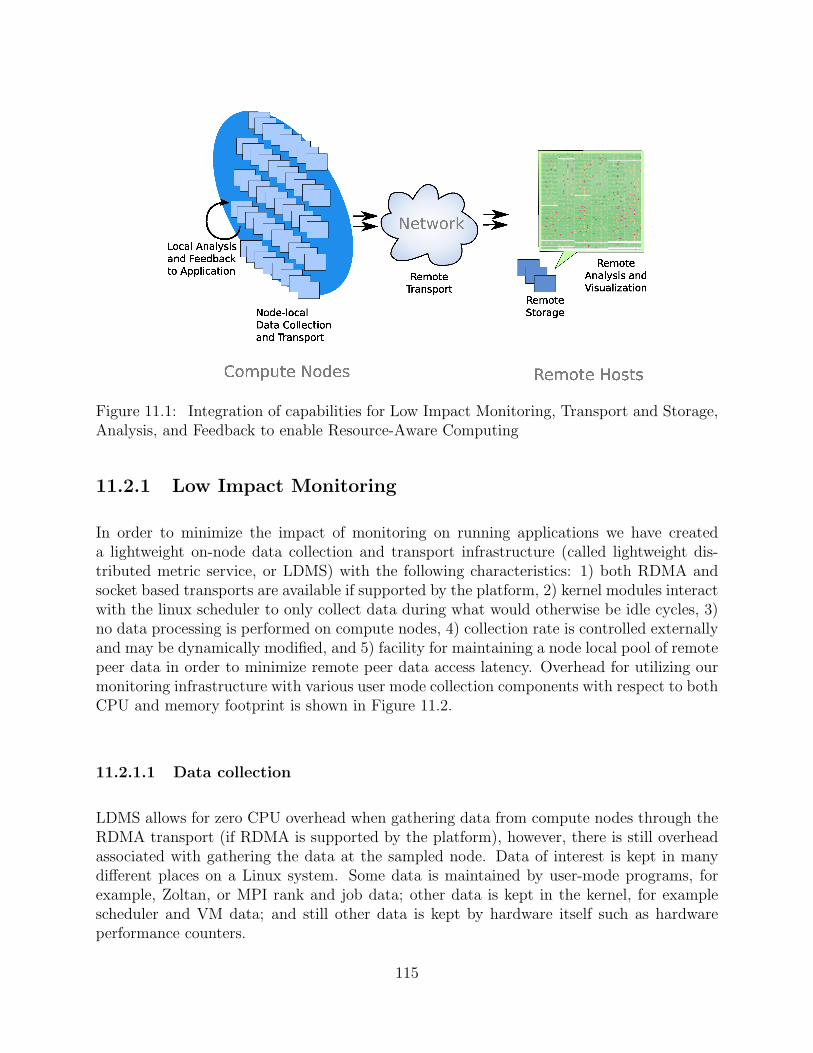
Figure 11.1: Integration of capabilities for Low Impact Monitoring, Transport and Storage,Analysis, and Feedback to enable Resource-Aware Computing

11.2.1 Low Impact Monitoring

In order to minimize the impact of monitoring on running applications we have createda lightweight on-node data collection and transport infrastructure (called lightweight dis-tributed metric service, or LDMS) with the following characteristics: 1) both RDMA andsocket based transports are available if supported by the platform, 2) kernel modules interactwith the linux scheduler to only collect data during what would otherwise be idle cycles, 3)no data processing is performed on compute nodes, 4) collection rate is controlled externallyand may be dynamically modified, and 5) facility for maintaining a node local pool of remotepeer data in order to minimize remote peer data access latency. Overhead for utilizing ourmonitoring infrastructure with various user mode collection components with respect to bothCPU and memory footprint is shown in Figure 11.2.

11.2.1.1 Data collection

LDMS allows for zero CPU overhead when gathering data from compute nodes through theRDMA transport (if RDMA is supported by the platform), however, there is still overheadassociated with gathering the data at the sampled node. Data of interest is kept in manydifferent places on a Linux system. Some data is maintained by user-mode programs, forexample, Zoltan, or MPI rank and job data; other data is kept in the kernel, for examplescheduler and VM data; and still other data is kept by hardware itself such as hardwareperformance counters.

115

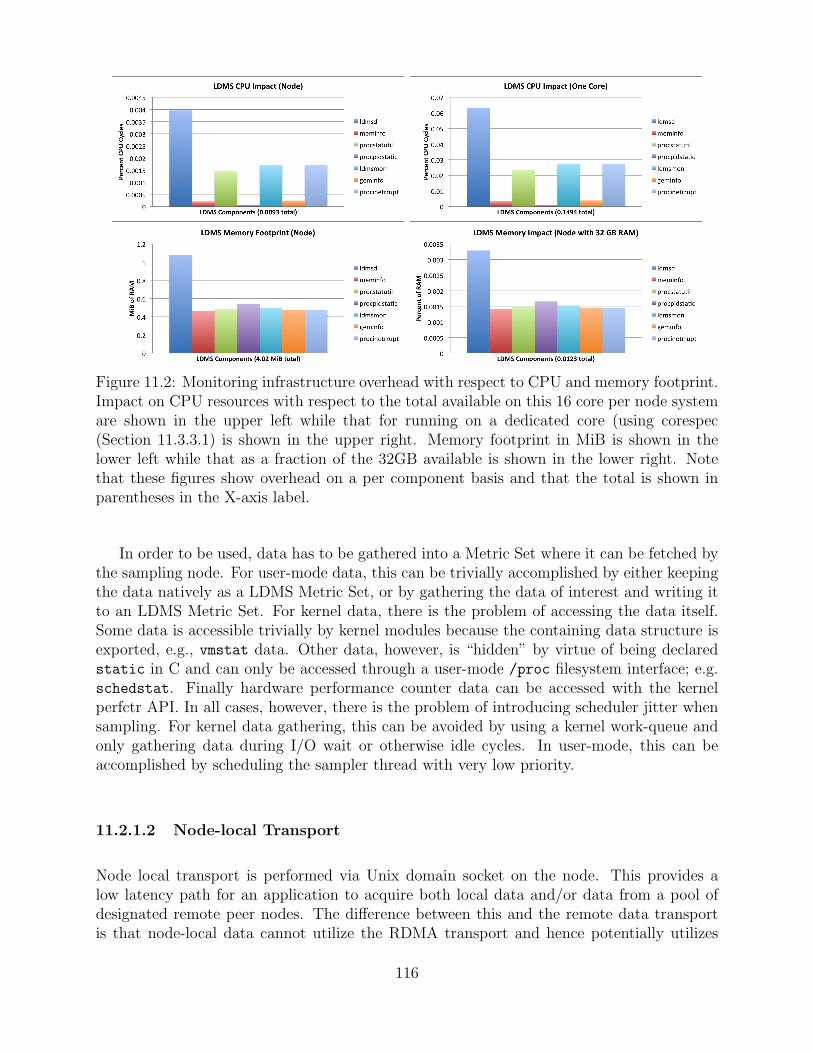
Figure 11.2: Monitoring infrastructure overhead with respect to CPU and memory footprint.Impact on CPU resources with respect to the total available on this 16 core per node systemare shown in the upper left while that for running on a dedicated core (using corespec(Section 11.3.3.1) is shown in the upper right. Memory footprint in MiB is shown in thelower left while that as a fraction of the 32GB available is shown in the lower right. Notethat these figures show overhead on a per component basis and that the total is shown inparentheses in the X-axis label.

In order to be used, data has to be gathered into a Metric Set where it can be fetched bythe sampling node. For user-mode data, this can be trivially accomplished by either keepingthe data natively as a LDMS Metric Set, or by gathering the data of interest and writing itto an LDMS Metric Set. For kernel data, there is the problem of accessing the data itself.Some data is accessible trivially by kernel modules because the containing data structure isexported, e.g., vmstat data. Other data, however, is “hidden” by virtue of being declaredstatic in C and can only be accessed through a user-mode /proc filesystem interface; e.g.schedstat. Finally hardware performance counter data can be accessed with the kernelperfctr API. In all cases, however, there is the problem of introducing scheduler jitter whensampling. For kernel data gathering, this can be avoided by using a kernel work-queue andonly gathering data during I/O wait or otherwise idle cycles. In user-mode, this can beaccomplished by scheduling the sampler thread with very low priority.

11.2.1.2 Node-local Transport

Node local transport is performed via Unix domain socket on the node. This provides alow latency path for an application to acquire both local data and/or data from a pool ofdesignated remote peer nodes. The difference between this and the remote data transportis that node-local data cannot utilize the RDMA transport and hence potentially utilizes

116

more CPU resources. However, node-local transport is expected to be utilized relativelyinfrequently (e.g. when an application is requesting data in order to evaluate a load balancingresponse) and hence will introduce insignificant overhead and/or jitter to the application asa whole.

11.2.2 Remote Transport and Storage

Remote transport of data is desirable for several reasons: 1) analysis of aggregations ofdata to understand statistical distributions, anomalous situations, and overall headroom forimprovement, 2) storage for comparison against data from other application runs, and 3)enabling low latency acquisition of a statistically meaningful set of peer node data for usein load balancing and scheduling decisions.

11.2.2.1 Remote transport

In order to minimize the impact of remote data transport on application processes runningon a node LDMS supports remote distributed memory access (RDMA) where hardware andsoftware permit. Thus a remote entity may access another node’s data as often as desiredwith no impact on running applications past an initial RDMA registration which may stayactive over the uptime of a node. Remote transport of data is performed using a pull modelin which the owning entity, whether it is the node on which the data is being collected or anintermediate transport node, is either completely passive (as in the case when using RDMA)or only sends a segment of data when it is requested (in the case where socket based transportis being used). Metadata and data generation numbers are used to ensure that informationbeing stored is both new and correct. In order to support socket based transport of dataacross asymmetric network boundaries we support two socket setup methods for accessingremote data. In order to describe these we define the “top” of a data stream to be thenode on which the data is collected and originates and the “bottom” to be the endpointfrom which the request for data is made. In this context “upstream” denotes closer to thedata source, or top, and “downstream” denotes closer to the data requester, or bottom. Ifa downstream LDMSD (LDMS daemon) entity is allowed to initiate a socket connectionwith his upstream neighbor LDMSD entity it is called “active” and does so directly. If,however, security profiles are such that a connection between two such entities can only beinitiated from upstream to downstream, then we utilize a “passive” LDMSD entity on thedownstream node which listens for a connection request from its upstream neighbor whichwe refer to as a “bridge” entity. Once the socket connection has been established the passiveLDMSD entity makes its requests for data from its upstream neighbor over this connectionin the same way an active LDMSD entity does. Note that these are persistent connectionsdue to the desire to minimize overhead i.e., we don’t want the overhead of negotiation forevery data request as these are expected to occur on sub- to few-second intervals.

117

11.2.2.2 Remote Storage

Constraints on storage on the remote host(s) include not only the ability to ingest dataat run-time rates, but also to represent that data in a way suitable for analysis. We havedeveloped a database backend, consisting of multiple, non-replicated databases. Analysesare performed on the databases in parallel, with the results aggregated to a common frontend. Details of the storage implementation are beyond the scope of this work, but can befound in [19]. In the exploratory phase of this work, we ingested samples of 1012 variables pernode from 556 compute nodes at a rate of 5 samples per second into 4 distributed databases.We expect that, after analysis, the necessary number of collected variables can be reducedsuch that an application run on the full Cielo system could be handled at the necessaryrate by the same 4 databases. For example 122 variables per node collected on 10 secondintervals across the whole Cielo system would require the same data ingestion rate as theexperimental work presented here.

11.2.3 Analysis

Our data analysis serves several functions: 1) provides understanding of how an applicationas a whole is utilizing the resources allocated to it in order to enable optimal matching ofapplication needs to resource requests on subsequent but similar application runs, 2) enabledynamic resource to load mapping over the course of an application run, and 3) comparison ofresource utilization/contention across processes, resources including nodes, and applicationruns to understand runtime variability and how utilization of data, analysis, and responsehas impacted both system resource utilization and application run time. We describe bothrun-time and post processing use of the data in the following subsections. Additionally webriefly describe the analysis role of our visualization component.

11.2.3.1 Post-processing

Before trying to dynamically adjust how an application is utilizing available resources itneeds to be determined if any adjustment is needed (i.e., is there a problem?) and, if so,what measurements should be taken into account, how each should be weighted, and whatfunctional aggregation should be performed. After these things are determined and imple-mented, application runs incorporating dynamic adjustment based on the implementationshould be compared against the baseline case to determine if there was improvement and ifthere might be room for more. Post-processing analysis of system state profiles related toapplication runs is used to address these use cases.

118

11.2.3.2 Run-time

Run-time analysis using our framework can be done in a node-local manner taking intoaccount information about both the local node and a peer node pool or remotely at thedata storage nodes as both locations have access to the same information. The tradeoffsfor these two modes of run-time analysis are latency, processing impact on application pro-cesses, and compute node memory footprint. While performing run-time analysis remotelyminimizes processing impact on application processes and compute node memory footprintit also presents a high latency path for response. Thus for low-latency response we performsmall computations on node, using the on-node data collection and local transport API toaccess data. In this work our run-time analysis was done in the context of dynamic loadpartitioning. Utilizing information gained in the post-processing analysis (Section 11.2.3.1),we determined a subset of variables to use in determining load imbalance and functionalforms for evaluating relative balance with respect to those variables. We then wrote smallfunctions that accessed only the necessary data to calculate the imbalance measures. Thoseresultant relative measures of load imbalance were then used in the run time repartitioningalgorithms (Section 11.2.4.2).

11.2.3.3 Visualization

Our visualization tool is useful for imparting qualitative understanding of balance and/orcontention in a running system. It enables a user to directly view raw measurables, such asCPU utilization, memory utilization, interrupts, context switches, etc., as a color-mappedvalue on a component. Simultaneously viewing these over all components being utilized byan application (including the operating system) provides a qualitative evaluation of how farout of balance a particular measurable is across all components and how that unfolds overtime. We also provide methods for rendering the time history of a small subset of values andfor statistical computations over ranges of time and components. This tool can be used forboth run-time and post data capture viewing of such information. Figure 11.3 is an exampleof using this tool for visualizing where system processes are running.

11.2.4 Application Feedback Methods

Our goal is that monitoring and analysis information be used to inform and/or triggerappropriate available system responses. Analysis or response mechanisms can call the nodelocal transport API for acquisition of both node local and peer node pool metrics of interestor use the remote analysis results. In this work we utilized both static and dynamic formsof feedback described in this section. Note that in this work all compute node and coreallocations are static for the duration of an application run and that in the context of thiswork dynamic feedback results in process load re-allocation.

119

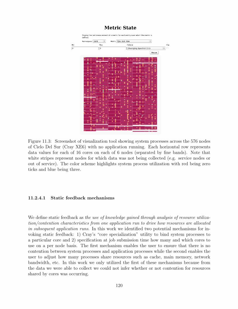
Figure 11.3: Screenshot of visualization tool showing system processes across the 576 nodesof Cielo Del Sur (Cray XE6) with no application running. Each horizontal row representsdata values for each of 16 cores on each of 6 nodes (separated by fine bands). Note thatwhite stripes represent nodes for which data was not being collected (e.g. service nodes orout of service). The color scheme highlights system process utilization with red being zeroticks and blue being three.

11.2.4.1 Static feedback mechanisms

We define static feedback as the use of knowledge gained through analysis of resource utiliza-tion/contention characteristics from one application run to drive how resources are allocatedin subsequent application runs. In this work we identified two potential mechanisms for in-voking static feedback: 1) Cray’s “core specialization” utility to bind system processes toa particular core and 2) specification at job submission time how many and which cores touse on a per node basis. The first mechanism enables the user to ensure that there is nocontention between system processes and application processes while the second enables theuser to adjust how many processes share resources such as cache, main memory, networkbandwidth, etc. In this work we only utilized the first of these mechanisms because fromthe data we were able to collect we could not infer whether or not contention for resourcesshared by cores was occurring.

120

11.2.4.2 Dynamic feedback mechanisms

We define dynamic feedback as the use of knowledge gained through analysis of resourceutilization/contention characteristics from both current and previous application runs to driverun-time resource allocation (including work to process allocation) for the current applicationrun. In order to enable dynamic workload to resource mapping, we targeted applicationswith facilities for redistribution of their workload during their runtime. In this work wechose applications in the Sierra [45] suite, which periodically call the Zoltan partitioner [40]to determine a new partitioning and which also have the facility to relocate data accordingly.

Zoltan contains a number of algorithms which assign objects to partitions, taking intoaccount specified object weights and partition sizes. Examples of the former include numberof elements or particles. In this work, we sought to define partition sizes, reflective of therelative ability of a resource to handle the workload assigned to it. We enhanced Zoltan to, atthe time of a partitioning calculation, make the appropriate calls to obtain variable data viaour on-node data collection API and calculate the partition sizes via the defined functionalform. These partition sizes were then used in the partitioning calculation as described inSection 11.2.3.2. The data movement to adjust the workload in response to the determinedpartitioning is handled by Sierra itself.

11.3 Applying the Infrastructure to Enable Resource-

Aware Computing

In this section we describe results of applying our infrastructure and tools as an integratedcapability to targeted application runs on several Cray XE6 systems including LANL’s Cielo.Here we describe characteristics of two applications we used and how our feedback mecha-nisms influenced dynamic run-time partitioning of their workload to process mapping.

11.3.1 Applications characteristics and experimental setup

In this work we targeted two codes: Aria [99] and Fuego [43, 42]. Aria is a thermal codeand thus the per-processor computational load is dependent on the number of elements inthe computation and less tied to the physical dynamics of the computation. As a result,significant dynamic load imbalance is not expected, however the Aria example code hasbeen shown to scale well to large numbers of processors. Fuego is a particle code whose per-processor computational load changes throughout the computation as particles move, areinjected, split, and/or removed. Repartitioning throughout the runtime thus redistributesthe mapping of particles to processors and rebalances the load. Rebalancing capabilities forsuch codes may potentially have significant benefit, however the particular Fuego exampleutilized here is limited in its scalability without significant additional tuning/investigationwhich was beyond the scope of this work.

121

The applications were run 1) on Cielo, with node-local analysis and feedback via Zoltan,and remote transport over DISCOM, an ASC wide-area high speed network, with remoteanalysis and storage on the ASC TLCC Whitney cluster at Sandia CA and 2) on a Cray XEplatform at Sandia NM, again with node-local analysis and feedback via Zoltan, with remotetransport to desktop machines at Sandia CA for analysis and storage. The Aria examplewas run with a process count of up to 10,112 while the Fuego example only scaled to the 64processes represented in this work.

11.3.2 Methodology used to search for appropriate indicators

Because we specifically targeted load imbalance and contention we were looking for data thatindicated evidence of wide variation of related metric values over processes of an application.This suggested that we target things with a large statistical variance. A problem with justcomputing mean and higher order moments on this type of data is that even for a singleprocess there is large variance on most dynamic metrics (CPU utilization, non-voluntarycontext switches, interrupts, etc.) over our sampling intervals of 5 to 10 seconds. Thuswe summed these values, on a per processor basis, over time windows commensurate withthe applications rebalancing interval, rather than our sampling interval, and examined thedistribution of these sums over all processes.

11.3.3 Aria measures of interest, feedback, and results

Due to the aforementioned static nature of Aria’s per process workload we first looked forindication of contention for resources. Analysis of several runs of our Aria example indicatedthat there were indeed metrics for which there was a wide distribution across processes, lowvariance for each particular process, and a high degree of correlation between system processcore affinity and application processes with large numbers of these metrics (non-voluntarycontext switches, interrupts, idle CPU, etc.). The ones which directly implied contentionwere non-voluntary context switches and interrupts. Since these would adversely impact thetime hardware resources are dedicated to the Aria application, we targeted these for usein the repartitioning calculation. (Note that the magnitude of counts of these are vastlydifferent and the impact of any occurrence on the application run time and memory evictionwas beyond the scope of this work.) This discovery drove the nature of the feedback andrun-time analyses utilized in conjunction with this application and described below.

11.3.3.1 Static feedback with Aria

In this case we utilized Cray’s “core specialization” (aka “corespec”) feature [38] which en-ables the user to specify that no system processes will be run on cores dedicated to applicationprocesses. This comes at the expense of having to give up a core per node (the default ofcore 15 was used in this case, but any core can be specified for this use) to host system

122

processes. We ran the same number of processes (8310) over 12% more nodes to accommo-date the loss of one core per node. The results show that non-voluntary context switches forapplication processes drop to zero and, though we expected slightly worse run-times givenmore inter-node communication, we obtained similar run-times presumably due to the highercost of more inter-node communication being offset by better per-node performance. Whilein this case we utilized all cores available for application use per node, indication of processcontention for shared cache, main memory, or network resources would be indicators thatsparser use of cores, to reduce the sharing of resources for which contention has been seen,would be in order.

11.3.3.2 Dynamic feedback with Aria

We utilized the Zoltan partitioner to implement dynamic feedback to both codes. As de-scribed in Section 11.2.4.2, Zoltan assigns objects to partitions, taking into account specifiedobject weights and partition sizes. In practice, in the targeted codes, the partition size isuniform. In contrast, in this work, we sought to define partition sizes, reflective of the relativeability of a resource to handle the workload assigned to it.

From an analysis perspective the measures of imbalance had to additionally be expressedin terms commensurate with the object weights. In this work we selected the number of non-voluntary context switches and the number of rescheduling interrupts to be used as measuresof contention in an expression for relative imbalance. We not only needed to determine afunctional form in which a greater number of non-voluntary context switches would result ina smaller partition size but also one scaled appropriately to still achieve a reasonable relativedistribution across all the partitions.

Using functional forms for partition sizes based on our post-run profiling, we ran ourapplications, with Zoltan repartitioning the workload per processor based on the data valuesexhibited at run time.

We first utilized the following function of two contention related metrics (non-voluntarycontext switches and rescheduling interrupts) to drive partitioning decisions in Aria fora 10,112 processor run on Cielo: for measures of contention c1 and c2 partitionsize =(c1 + c2) ∗ (100)/max(c1 + c2) with a floor of 1 and a ceiling of 100. The measures ofcontention are evaluated from values after the previous rebalancing step to the current re-balancing calculation. At run time, non-voluntary context switches and interrupts occurredpreferentially on cores 0 and 9 across all nodes. Our run-time feedback thus resulted insmaller partitions on those cores, however our functional form resulted in too great a rangeof partition sizes to derive benefit in this particular run. Additional tuning of the parametersof the functional form would be required in order to reduce the range appropriately.

Likewise we utilized the following function of CPU related metrics to drive partitioningdecisions as a result of imbalance in CPU utilization by an 8310 processor Aria run on San-dia’s Cielo Del Sur (CDS): partitionsize = [(usertime+systemtime+idletime)/(usertime+systemtime)]. The times are measured in ticks between after the previous rebalancing step to

123

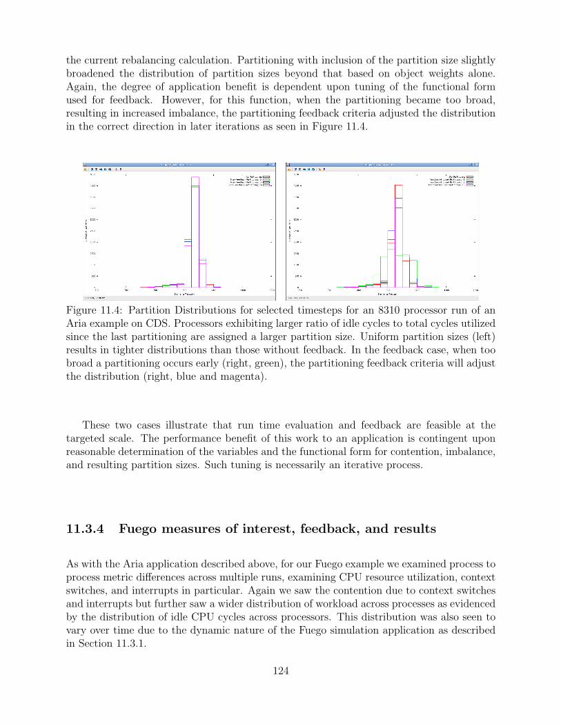
the current rebalancing calculation. Partitioning with inclusion of the partition size slightlybroadened the distribution of partition sizes beyond that based on object weights alone.Again, the degree of application benefit is dependent upon tuning of the functional formused for feedback. However, for this function, when the partitioning became too broad,resulting in increased imbalance, the partitioning feedback criteria adjusted the distributionin the correct direction in later iterations as seen in Figure 11.4.

Figure 11.4: Partition Distributions for selected timesteps for an 8310 processor run of anAria example on CDS. Processors exhibiting larger ratio of idle cycles to total cycles utilizedsince the last partitioning are assigned a larger partition size. Uniform partition sizes (left)results in tighter distributions than those without feedback. In the feedback case, when toobroad a partitioning occurs early (right, green), the partitioning feedback criteria will adjustthe distribution (right, blue and magenta).

These two cases illustrate that run time evaluation and feedback are feasible at thetargeted scale. The performance benefit of this work to an application is contingent uponreasonable determination of the variables and the functional form for contention, imbalance,and resulting partition sizes. Such tuning is necessarily an iterative process.

11.3.4 Fuego measures of interest, feedback, and results

As with the Aria application described above, for our Fuego example we examined process toprocess metric differences across multiple runs, examining CPU resource utilization, contextswitches, and interrupts in particular. Again we saw the contention due to context switchesand interrupts but further saw a wider distribution of workload across processes as evidencedby the distribution of idle CPU cycles across processors. This distribution was also seen tovary over time due to the dynamic nature of the Fuego simulation application as describedin Section 11.3.1.

124

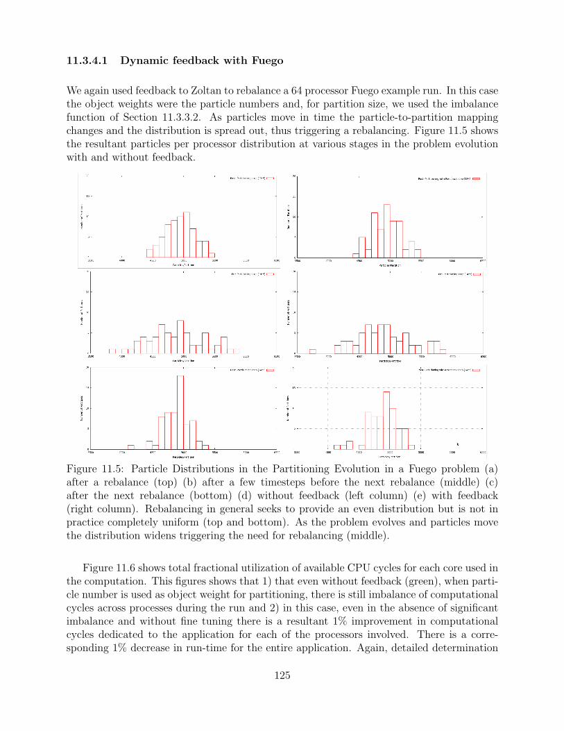
11.3.4.1 Dynamic feedback with Fuego

We again used feedback to Zoltan to rebalance a 64 processor Fuego example run. In this casethe object weights were the particle numbers and, for partition size, we used the imbalancefunction of Section 11.3.3.2. As particles move in time the particle-to-partition mappingchanges and the distribution is spread out, thus triggering a rebalancing. Figure 11.5 showsthe resultant particles per processor distribution at various stages in the problem evolutionwith and without feedback.

Figure 11.5: Particle Distributions in the Partitioning Evolution in a Fuego problem (a)after a rebalance (top) (b) after a few timesteps before the next rebalance (middle) (c)after the next rebalance (bottom) (d) without feedback (left column) (e) with feedback(right column). Rebalancing in general seeks to provide an even distribution but is not inpractice completely uniform (top and bottom). As the problem evolves and particles movethe distribution widens triggering the need for rebalancing (middle).

Figure 11.6 shows total fractional utilization of available CPU cycles for each core used inthe computation. This figures shows that 1) that even without feedback (green), when parti-cle number is used as object weight for partitioning, there is still imbalance of computationalcycles across processes during the run and 2) in this case, even in the absence of significantimbalance and without fine tuning there is a resultant 1% improvement in computationalcycles dedicated to the application for each of the processors involved. There is a corre-sponding 1% decrease in run-time for the entire application. Again, detailed determination

125

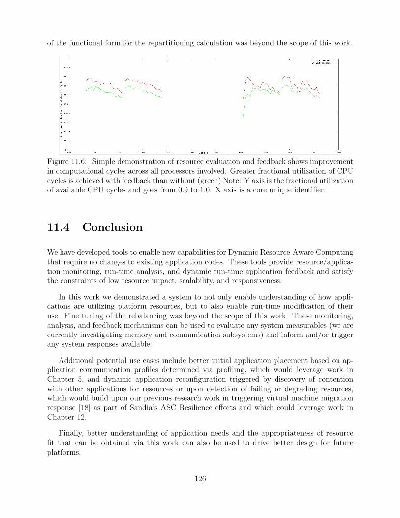
of the functional form for the repartitioning calculation was beyond the scope of this work.

Figure 11.6: Simple demonstration of resource evaluation and feedback shows improvementin computational cycles across all processors involved. Greater fractional utilization of CPUcycles is achieved with feedback than without (green) Note: Y axis is the fractional utilizationof available CPU cycles and goes from 0.9 to 1.0. X axis is a core unique identifier.

11.4 Conclusion

We have developed tools to enable new capabilities for Dynamic Resource-Aware Computingthat require no changes to existing application codes. These tools provide resource/applica-tion monitoring, run-time analysis, and dynamic run-time application feedback and satisfythe constraints of low resource impact, scalability, and responsiveness.

In this work we demonstrated a system to not only enable understanding of how appli-cations are utilizing platform resources, but to also enable run-time modification of theiruse. Fine tuning of the rebalancing was beyond the scope of this work. These monitoring,analysis, and feedback mechanisms can be used to evaluate any system measurables (we arecurrently investigating memory and communication subsystems) and inform and/or triggerany system responses available.

Additional potential use cases include better initial application placement based on ap-plication communication profiles determined via profiling, which would leverage work inChapter 5, and dynamic application reconfiguration triggered by discovery of contentionwith other applications for resources or upon detection of failing or degrading resources,which would build upon our previous research work in triggering virtual machine migrationresponse [18] as part of Sandia’s ASC Resilience efforts and which could leverage work inChapter 12.

Finally, better understanding of application needs and the appropriateness of resourcefit that can be obtained via this work can also be used to drive better design for futureplatforms.

126

Chapter 12

A Scalable VirtualizationEnvironment for Exascale

Abstract: Hardware-accelerated virtualization support has become ubiquitous on mod-ern computing platforms, driven primarily by the requirements of the data center and cloudcomputing industries. This technology also has compelling use-cases for exascale computing,such as using guest operating systems to deploy specialized compute node functionality on-the-fly (e.g., for visualization or in-transit data analysis), providing backwards-compatibilityto existing MPI applications running on exascale systems via “legacy” virtual machine en-vironments, and leveraging the full-system view of the virtualization layer to facilitate themapping of abstract machine models to the available physical hardware. As a step towardsrealizing these use-cases and others, we have been developing a scalable virtual machinemonitor that augments the traditional fixed software stack provided by vendors. We havedeployed this system on Red Storm and evaluated the performance of the CTH and Sageapplications running inside of a virtual machine on up to 4096 compute nodes. The resultsshow that the overhead induced by our virtualization layer is low, typically less than 5%,proving the feasibility of running communication intensive, tightly coupled applications in avirtual machine environment.

12.1 Introduction

Current supercomputers provide a fixed software environment that is typically limited inits functionality for performance and scalability reasons. Examples include the Red Stormsystem at Sandia and the BlueGene/L system at LLNL, which both use custom lightweightkernel (LWK) operating systems that provide only the functionality needed to support scal-able parallel applications. If an application requires more functionality than is available, itmust be reworked to eliminate the dependencies or not be able to make use of the system.

Together with collaborators at Northwestern University and the University of New Mex-ico, we have been working to address this issue by developing a virtual machine monitor(VMM) that can be embedded in a traditional LWK operating system. Specifically, we haveembedded the Palacios VMM developed at Northwestern inside of Sandia’s Kitten LWK(Figure 12.1). The VMM capability enables users to dynamically replace the normal fixed

127

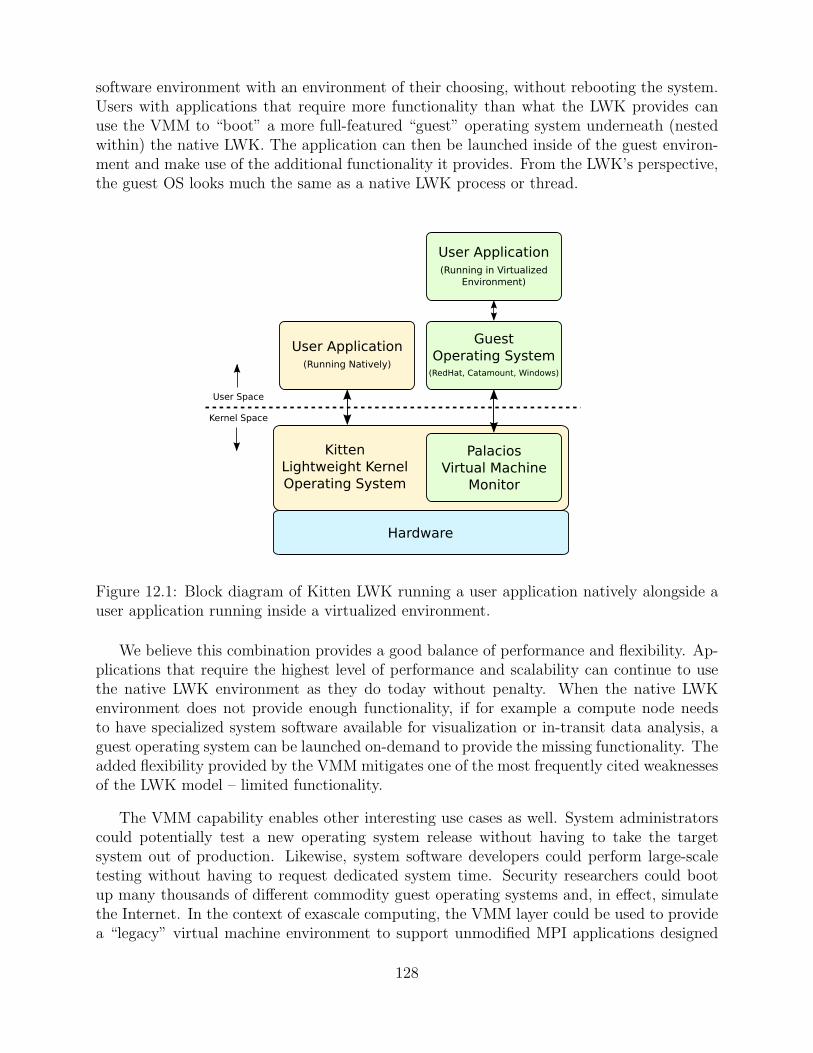
software environment with an environment of their choosing, without rebooting the system.Users with applications that require more functionality than what the LWK provides canuse the VMM to “boot” a more full-featured “guest” operating system underneath (nestedwithin) the native LWK. The application can then be launched inside of the guest environ-ment and make use of the additional functionality it provides. From the LWK’s perspective,the guest OS looks much the same as a native LWK process or thread.

Hardware

User Space

Kernel Space

PalaciosVirtual Machine

Monitor

KittenLightweight KernelOperating System

GuestOperating System

(RedHat, Catamount, Windows)

User Application

(Running Natively)

User Application

(Running in VirtualizedEnvironment)

Figure 12.1: Block diagram of Kitten LWK running a user application natively alongside auser application running inside a virtualized environment.

We believe this combination provides a good balance of performance and flexibility. Ap-plications that require the highest level of performance and scalability can continue to usethe native LWK environment as they do today without penalty. When the native LWKenvironment does not provide enough functionality, if for example a compute node needsto have specialized system software available for visualization or in-transit data analysis, aguest operating system can be launched on-demand to provide the missing functionality. Theadded flexibility provided by the VMM mitigates one of the most frequently cited weaknessesof the LWK model – limited functionality.

The VMM capability enables other interesting use cases as well. System administratorscould potentially test a new operating system release without having to take the targetsystem out of production. Likewise, system software developers could perform large-scaletesting without having to request dedicated system time. Security researchers could bootup many thousands of different commodity guest operating systems and, in effect, simulatethe Internet. In the context of exascale computing, the VMM layer could be used to providea “legacy” virtual machine environment to support unmodified MPI applications designed

128

for prior-generation supercomputers. The extra layer of indirection provided by the VMMlayer makes it a powerful tool for mapping abstract machine models, such as a “legacy”distributed memory massively parallel machine model, to the available underlying physicalhardware, which may be substantially different than what is exposed to software.

12.2 Application Results

The price of the added flexibility afforded by the VMM is increased overhead in the vir-tualized environment compared to native execution. The extra level of indirection in theVMM and virtualization hardware necessarily adds some overhead. In order to evaluate thisoverhead we performed experiments on 2048 nodes of Red Storm with two real applications– the CTH [44] hydrocode and Sage [74] adaptive grid Eulerian hydrocode – comparing per-formance executing natively to performance executing within the virtualized environmentprovided by Kitten and Palacios. To the best of our knowledge, these are the only virtual-ization experiments performed on a peta-flop class architecture – Cray XT – and are by farthe largest scale experiments performed to-date. Previous studies have used a maximum of128 nodes and have only considered benchmarks, not real applications.

Figure 12.2 compares the performance of CTH and Sage executing natively on Red Storm,in the Catamount LWK, to their performance executing within Catamount running as aguest operating system on top of Kitten and Palacios. The results show that the virtualizedenvironment adds less than 5% overhead in all cases, even at the highest scales tested. Thisdemonstrates for the first time the feasibility of running communication intensive, tightlycoupled applications such as these within a modern virtualized parallel environment.

Additionally, we evaluated two memory management schemes for the virtualized envi-ronment. With shadow paging, the Palacios VMM is responsible for memory management(memory management is performed in software). With nested paging, virtualization hard-ware in the host processor performs memory management. The results indicate, counterintuitively, that software memory management is slightly faster than hardware memorymanagement for these HPC workloads. This was found to be due to extra overheads in theprocessor’s translation lookaside buffer (TLB) when using nested paging.

12.3 Conclusion

The end goal of this research is to provide users with a more flexible supercomputer en-vironment without requiring the most scalable applications – those that work best in aLWK environment – to sacrifice performance. Given the promising results on Red Storm,we hope to deploy this technology in future capability supercomputer platforms. For moreinformation about Kitten and Palacios, see [78].

129

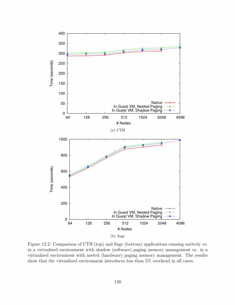
0

50

100

150

200

250

300

350

400

64 128 256 512 1024 2048 4096

Tim

e (

se

co

nd

s)

# Nodes

NativeIn Guest VM, Nested Paging

In Guest VM, Shadow Paging

(a) CTH

0

200

400

600

800

1000

64 128 256 512 1024 2048 4096

Tim

e (

se

co

nd

s)

# Nodes

NativeIn Guest VM, Nested Paging

In Guest VM, Shadow Paging

(b) Sage

Figure 12.2: Comparison of CTH (top) and Sage (bottom) applications running natively vs.in a virtualized environment with shadow (software) paging memory management vs. in avirtualized environment with nested (hardware) paging memory management. The resultsshow that the virtualized environment introduces less than 5% overhead in all cases.

130

Chapter 13

Goofy File System forHigh-Bandwidth Checkpoints

Abstract: The Goofy File System, a file system for exascale under active development,is designed to allow the storage software to maximize quality of service through increasedflexibility and local decision-making. By allowing the storage system to manage a rangeof storage targets that have varying speeds and capacities, the system can increase thespeed and surety of storage to the application. We instrument CTH to use a group ofRAM-based GoofyFS storage servers allocated within the job as a high-performance storagetier to accept checkpoints, allowing computation to potentially continue asynchronously ofcheckpoint migration to slower, more permanent storage. The result is a 10-60x speedup inconstructing and moving checkpoint data from the compute nodes.

13.1 Introduction and Motivation

GoofyFS is a peer-to-peer-inspired file system for exascale under active development. It ispart of a multi-year effort among Sandia National Laboratories, the University of Alabama atBirmingham, Clemson University, and Argonne National Laboratory. The motivation behindGoofyFS is that, as HPC systems (and their storage systems) grow, increasing componentcounts will imply a growth in the number of device failures. The storage system will be insome sort of failure mode at all times, requiring it to adapt dynamically to its own health.Peer-to-peer systems are well known for their ability to provide resilience by handling clientturnover [131], and provide a ripe area of exploration to improve large scale storage systems.

Resilience and performance concerns influence the design of GoofyFS in a number ofways. First, data should be automatically migrated and replicated through the system tomaintain data integrity. For example, if data is replicated among three servers, and onefails, data may be replicated immediately without central coordination to another server orset of servers, ensuring that at least three copies remain. Second, data may be relocatedor replicated for performance reasons, including to and from a set of compute nodes thathold data in RAM as the fastest tier in a caching model. Finally, clients may write datato any server that provides the client with high quality of service quantified by bandwidth,reliability, I/O operations per second, latency, and so on.

131

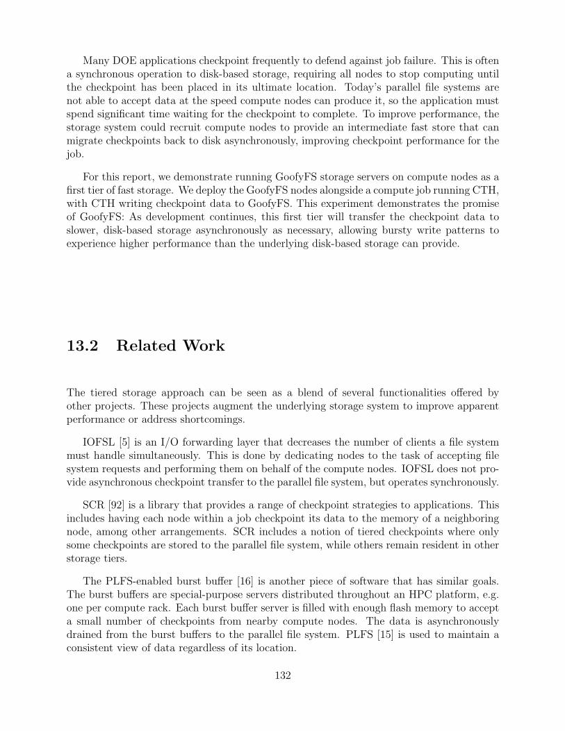
Many DOE applications checkpoint frequently to defend against job failure. This is oftena synchronous operation to disk-based storage, requiring all nodes to stop computing untilthe checkpoint has been placed in its ultimate location. Today’s parallel file systems arenot able to accept data at the speed compute nodes can produce it, so the application mustspend significant time waiting for the checkpoint to complete. To improve performance, thestorage system could recruit compute nodes to provide an intermediate fast store that canmigrate checkpoints back to disk asynchronously, improving checkpoint performance for thejob.

For this report, we demonstrate running GoofyFS storage servers on compute nodes as afirst tier of fast storage. We deploy the GoofyFS nodes alongside a compute job running CTH,with CTH writing checkpoint data to GoofyFS. This experiment demonstrates the promiseof GoofyFS: As development continues, this first tier will transfer the checkpoint data toslower, disk-based storage asynchronously as necessary, allowing bursty write patterns toexperience higher performance than the underlying disk-based storage can provide.

13.2 Related Work

The tiered storage approach can be seen as a blend of several functionalities offered byother projects. These projects augment the underlying storage system to improve apparentperformance or address shortcomings.

IOFSL [5] is an I/O forwarding layer that decreases the number of clients a file systemmust handle simultaneously. This is done by dedicating nodes to the task of accepting filesystem requests and performing them on behalf of the compute nodes. IOFSL does not pro-vide asynchronous checkpoint transfer to the parallel file system, but operates synchronously.

SCR [92] is a library that provides a range of checkpoint strategies to applications. Thisincludes having each node within a job checkpoint its data to the memory of a neighboringnode, among other arrangements. SCR includes a notion of tiered checkpoints where onlysome checkpoints are stored to the parallel file system, while others remain resident in otherstorage tiers.

The PLFS-enabled burst buffer [16] is another piece of software that has similar goals.The burst buffers are special-purpose servers distributed throughout an HPC platform, e.g.one per compute rack. Each burst buffer server is filled with enough flash memory to accepta small number of checkpoints from nearby compute nodes. The data is asynchronouslydrained from the burst buffers to the parallel file system. PLFS [15] is used to maintain aconsistent view of data regardless of its location.

132

13.3 The GoofyFS Storage Server and Client

The GoofyFS storage server provides an object-based storage API. Each object has a 128-bitidentifier and a 64-bit address space. The storage server supports sparse objects and con-flict resolution of objects via update identifiers. The API is RDMA-based, as the networklayer (Single-Sided Messaging, or SSM [51]) is heavily influenced by the Portals 4.0 specifi-cation [120]. For this experiment, SSM used an MPI-based transport layer, but others areunder active development.

No generally useful POSIX-like client exists for GoofyFS. While a FUSE-based client hasbeen demonstrated as a proof-of-concept, it is not meant for use by applications. Instead, asimple custom client was crafted for CTH that stores checkpoint data with a file per object,with a one megabyte local buffer to ensure that larger messages are sent to the storage serveras needed. Because CTH’s checkpoints have predictable names based on the iteration andrank of the process, a job ID and rank can be used to derive a unique object ID. A morefriendly POSIX client for HPC is under development.

13.4 Instrumenting CTH

To give CTH access to GoofyFS servers in the Cielo application environment, we launchedextra processes within the CTH allocation specifically dedicated to GoofyFS. Where CTHcalls MPI Init, we inserted a call to our own initialization routine that created a global com-municator, splitting the nodes between a CTH group and a GoofyFS group. The GoofyFSprocesses were instructed to enter an event loop to satisfy storage requests, while the CTHnodes were released to participate in the compute job normally. A number of operations CTHperformed over and within MPI COMM WORLD had to be changed to use the new communicator.

Other changes were less invasive. To have CTH use GoofyFS’s storage protocol, weleveraged syncio, an alternative I/O infrastructure already present in CTH. Syncio optionallycoordinates I/O from nodes so that storage servers in certain previous platforms would notbe overloaded from many simultaneous I/O requests from CTH. Syncio’s API includes read,write, open, and close, creating a straightforward mapping of common I/O tasks. As Cielodoes not require syncio functionality, we created simple replacements of those routines thatwould interact with the GoofyFS storage servers directly. A small number of further changeshad to be made to routines that were not written to use syncio.

We evenly distributed nodes running GoofyFS processes throughout the CTH job. Specif-ically, we treat the nodes in the job in groups of five, where each group k contains the processIDs between k × 80 and (k + 1) × 80 − 1, inclusive. The lowest 16 ranks, which are locatedin the first node of the group, run GoofyFS server instances. The highest 64 ranks, whichcomprise the other four nodes of the group, run CTH processes.

The CTH processes are directly mapped to the GoofyFS processes in the first node of

133

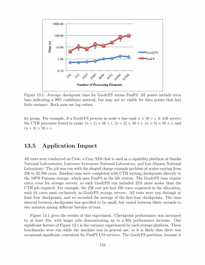
0.10

1.00

10.00

100.00

1000.00

256

512

1024

20

48

4096

81

92

1638

4

3276

8

Tim

e (s

)

Number of Processing Elements

GoofyFS

PanFS

Figure 13.1: Average checkpoint time for GoofyFS versus PanFS. All points include errorbars indicating a 99% confidence interval, but may not be visible for data points that hadlittle variance. Both axes use log values.

its group. For example, if a GoofyFS process in node n has rank n × 16 + i, it will servicethe CTH processes found in ranks (n + 1) × 16 + i, (n + 2) × 16 + i, (n + 3) × 16 + i, and(n + 4) × 16 + i.

13.5 Application Impact

All tests were conducted on Cielo, a Cray XE6 that is used as a capability platform at SandiaNational Laboratories, Lawrence Livermore National Laboratory, and Los Alamos NationalLaboratory. The job was run with the shaped charge example problem at scales varying from256 to 32,768 cores. Baseline runs were completed with CTH writing checkpoints directly tothe 10PB Panasas storage, which uses PanFS as the file system. The GoofyFS runs requireextra cores for storage servers, so each GoofyFS run included 25% more nodes than theCTH job required. For example, the 256 core job had 320 cores requested in the allocation,with 64 cores used exclusively as GoofyFS storage servers. All tests were run through atleast four checkpoints, and we recorded the average of the first four checkpoints. The timeinterval between checkpoints was specified to be small, but varied between thirty seconds totwo minutes among different batches of runs.

Figure 13.1 gives the results of this experiment. Checkpoint performance was increasedby at least 10x, with larger jobs demonstrating up to a 60x performance increase. Onesignificant feature of Figure 13.1 is the variance experienced by each storage platform. Thesebenchmarks were run while the machine was in general use, so it is likely that there wasoccasional significant contention for PanFS I/O services. The GoofyFS partition, because it

134

is dedicated to a single job, displayed almost no variance.

While these jobs used a rather large 25% increase in allocation of nodes per job, thiswas a decision made to ensure that each node had enough space available for checkpointstorage. CTH compresses its checkpoints, causing some processes to write much more datathan others. With a good mechanism for load balancing, and implementation of data mi-gration capability, it may be possible to exploit a much smaller fraction of servers with goodperformance.

13.6 Conclusion

This demonstration of early GoofyFS functionality shows a significant benefit for a real I/Oworkload, checkpointing, in a real application, CTH. By running GoofyFS storage serverswithin a job as RAM-only stores, CTH was able to store checkpoints 10-60x faster thanstoring to PanFS, allowing the job to continue computing sooner. While this prototypedid not include automatic data migration, the checkpoint was available to be pushed orpulled to disk-based storage as needed after the compute nodes continued computing. Futuredevelopments include the ability to dynamically spawn GoofyFS nodes to absorb checkpoints,expanding this mechanism to other fast tiers of storage like flash memory, and sharing ofdynamic GoofyFS nodes between multiple jobs as needed.

135

136

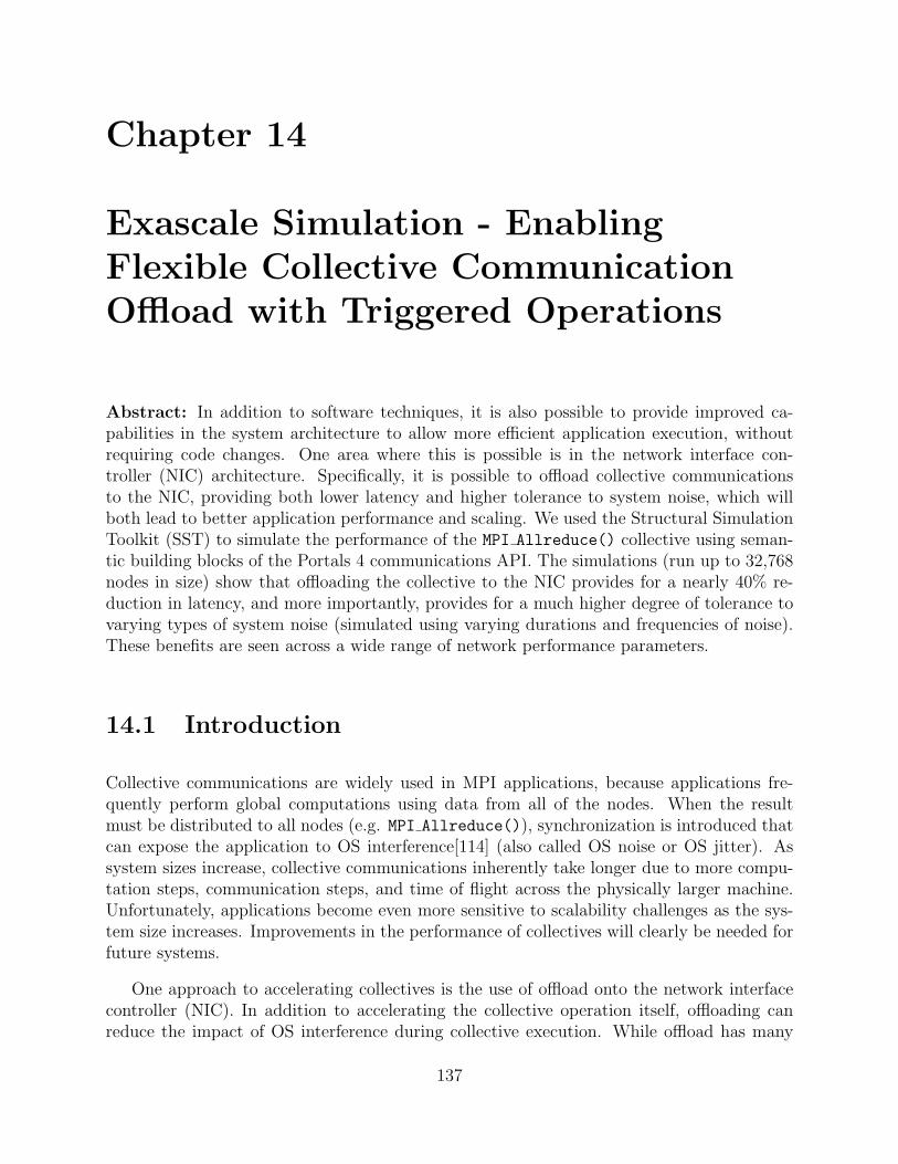
Chapter 14

Exascale Simulation - EnablingFlexible Collective CommunicationOffload with Triggered Operations

Abstract: In addition to software techniques, it is also possible to provide improved ca-pabilities in the system architecture to allow more efficient application execution, withoutrequiring code changes. One area where this is possible is in the network interface con-troller (NIC) architecture. Specifically, it is possible to offload collective communicationsto the NIC, providing both lower latency and higher tolerance to system noise, which willboth lead to better application performance and scaling. We used the Structural SimulationToolkit (SST) to simulate the performance of the MPI Allreduce() collective using seman-tic building blocks of the Portals 4 communications API. The simulations (run up to 32,768nodes in size) show that offloading the collective to the NIC provides for a nearly 40% re-duction in latency, and more importantly, provides for a much higher degree of tolerance tovarying types of system noise (simulated using varying durations and frequencies of noise).These benefits are seen across a wide range of network performance parameters.

14.1 Introduction

Collective communications are widely used in MPI applications, because applications fre-quently perform global computations using data from all of the nodes. When the resultmust be distributed to all nodes (e.g. MPI Allreduce()), synchronization is introduced thatcan expose the application to OS interference[114] (also called OS noise or OS jitter). Assystem sizes increase, collective communications inherently take longer due to more compu-tation steps, communication steps, and time of flight across the physically larger machine.Unfortunately, applications become even more sensitive to scalability challenges as the sys-tem size increases. Improvements in the performance of collectives will clearly be needed forfuture systems.

One approach to accelerating collectives is the use of offload onto the network interfacecontroller (NIC). In addition to accelerating the collective operation itself, offloading canreduce the impact of OS interference during collective execution. While offload has many

137

attractive aspects, current implementations show some drawbacks as well. Network adaptersare typically not easy to program to experiment with new collective algorithms. In manycases, the programmable resources that are available have significantly lower performancethan the host processor[93, 136]. Rather than adding fixed-function hardware to implementa single collective algorithm, it is desirable to expose a semantic building block that canimplement multiple collective algorithms for multiple upper-level libraries, including MPI.Given all of the potential factors used in determining an optimal collective algorithm, suchas process arrival[50], the ability to implement the algorithm on the host while offloading acollective can be advantageous.

We recently incorporated the concept of triggered operations, including triggered remotewrites and triggered remote atomic operations, into the Portals 4[121] network programminginterface. Triggered operations allow an application to setup a communication operation thatwill be issued in the future by the NIC when a trigger condition is met. Triggered operationsrequire a new type of event to provide efficient tracking of message completion to use asa trigger condition. We introduce counting events that can be used in combination with athreshold to trigger operations. As soon as an application initiates a collective communica-tion, the MPI library on each node can set up all message transactions that will be requiredfor the entire collective operation and then simply wait for completion of all of the messagerequests. This approach allows the application to provide the algorithm and higher-levelfunctions, while the NIC offloads the message processing and arithmetic operations. Theflexibility of host-based algorithms and the host-based development cycle are maintainedwith the performance advantages of collective offload.

One commonly used collective operation is MPI Allreduce()[136, 93]. MPI Allreduce()

is frequently used for a small number of data items (often only one) with a simple arithmeticoperation (often minimum or maximum). This paper describes the triggered operationsneeded to implement MPI Allreduce() and how MPI Allreduce() is implemented usingthose operations. A performance analysis is used to explain how the use of triggered oper-ations can impact collective algorithm design. In addition, simulations are used to presentthe performance impact of collective offload using triggered operations, including how thetolerance to OS noise of the collective operation is impacted by offload.

14.2 Triggered Operations in Portals 4

Portals 4[121] added two semantic building blocks to support the efficient offload of col-lectives. Counting events enable lightweight tracking of operation completion. Triggeredoperations leverage counting events to defer the start of an operation until a threshold isreached. Together, these constructs allow software on the host to chain new outgoing oper-ations as responses to incoming operations.

The semantics of counting events are simple: when an operation completes, a counter isincremented in application memory. Counting events can be associated with any operation.

138

Triggered operations leverage counting events to allow the application to create dependencychains through several operations. The standard form of a triggered operation is to add acounting event handle and threshold value to the standard arguments for the correspondingPortals call. A triggered operation can be passed from the application to the networkinterface when the triggered operation call occurs, but the network interface does not retrievethe data from memory and send the message until the associated counting event reaches thespecified threshold.

14.3 Evaluation Methodology

The Structural Simulation Toolkit (SST) v2.0 was used to simulate both a host-based and anoffloaded version of two algorithms that implement MPI Allreduce(). A torus network of upto 32K nodes (32×32×32) was simulated. Simulations were run with and without simulatedOS interference to determine the success of offloaded implementations in eliminating noise.

14.3.1 Algorithms for Allreduce

Many applications use MPI Allreduce() to perform a global operation on floating-pointinputs. Unfortunately, floating-point numbers are not associative. As such, there are twoalgorithms that are prevalently used for MPI Allreduce() to insure that all participantsreceive the same result: a tree-based algorithm and a recursive doubling algorithm.

The classic allreduce implementation is a reduction followed by a broadcast, using a tree-based communication topology. We used a binomial tree, in which nodes toward the top ofthe tree do more work than nodes toward the bottom of the tree. The binomial tree provedmore efficient in both host-based and triggered implementations than a strict binary tree.

The recursive doubling allreduce algorithm [116] uses a butterfly communication patternand redundant calculations to reduce the number of communication steps compared to atree algorithm. The recursive doubling algorithm is an optimization for small input vectors,where the cost of communication is latency dominated and outweighs the cost of redundantcalculations. Whereas the binomial tree algorithm has 2log(N) communication steps witheach step involving a smaller number of processors, the recursive doubling algorithm performslog(N) steps, with each step involving every node.

14.3.1.1 Implementation with Triggered Operations

Figure 14.1 illustrates the functions used in the pseudo-code examples. Only the subset ofthe standard Portals arguments that are most relevant are shown in Figure 14.1. As shownin the figure, data movement operations take a source memory descriptor (a handle to a localmemory region). The “Portal Table Index” is used like a protocol switch — conceptually

139

PtlTriggeredAtomic(source md h, //source of data on local nodedestination, //target node IDpt index, //Portal table index (target buffer)op, dtype, //operation and datatypetrigger ct h,//counting event to trigger onthreshold); //trigger threshold

PtlTriggeredPut(source md h, //source of data on local nodedestination, //target node IDpt index, //Portal table index (target buffer)trigger ct h,//counting event to trigger onthreshold); //trigger threshold

PtlAtomic(source md h, //source of data on local nodedestination, //target node IDpt index, //Portal table index (target buffer)op, dtype); //operation and datatype

PtlTriggeredCTInc(modify ct h, //counting event to incrementincrement, //increment valuetrigger ct h, //counting event to trigger onthreshold); //trigger threshold

PtlCTWait(wait ct h, //counting event to wait onthreshold);//wait until this threshold

Figure 14.1: Function definitions for Portals pseudo-code

similar to a TCP/IP port — in Portals and is used to segregate phases of an algorithm.Atomic operations take an operation and datatype argument, which includes such thingsas double precision floating-point. Finally, triggered operations require arguments for thecounter to be monitored and the threshold at which it triggers.

Figure 14.2 shows implementations of the tree-based and recursive doubling allreducealgorithms using triggered operations. In the tree-based algorithm, Leaf nodes push con-tributions directly to their parent node and wait for an answer to arrive. Other nodesatomically add their local contribution to a temporary buffer, and when data is receivedfrom all children, send the aggregated contribution to their parent node. In the recursivedoubling algorithm, each pair of participants at level A add their contributions in bouncebuffer A, and a triggered operation atomically adds that answer to bounce buffer A + 1 forthe next iteration. After log(N) iterations, each node has the final result of the allreduce.

14.3.2 Structural Simulation Toolkit v2.0

The Structural Simulation Toolkit v2.0 (SST) [133] provides a component-based simulationenvironment designed for simulating large-scale HPC environments. The simulator is de-signed to be flexible enough to simultaneously provide both cycle-accurate and event-basedsimulation environments. The simulations presented utilize a cycle-accurate router networkmodel, based on the Cray SeaStar router, combined with a high-level, event-driven networkinterface and host processor model.

14.3.3 Simulated Architecture

The network interface architecture that was simulated is shown in Figure 14.3. Portions ofPortals processing is offloaded to the network interface, including the processing of incoming

140

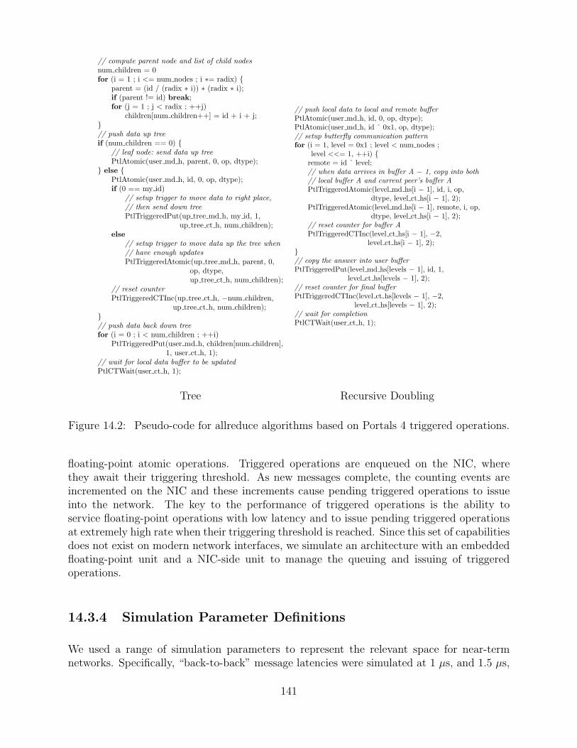
// compute parent node and list of child nodesnum children = 0for (i = 1 ; i <= num nodes ; i ∗= radix) {

parent = (id / (radix ∗ i)) ∗ (radix ∗ i);if (parent != id) break;for (j = 1 ; j < radix ; ++j)

children[num children++] = id + i + j;}// push data up treeif (num children == 0) {

// leaf node: send data up treePtlAtomic(user md h, parent, 0, op, dtype);

} else {PtlAtomic(user md h, id, 0, op, dtype);if (0 == my id)

// setup trigger to move data to right place,// then send down treePtlTriggeredPut(up tree md h, my id, 1,

up tree ct h, num children);else

// setup trigger to move data up the tree when// have enough updatesPtlTriggeredAtomic(up tree md h, parent, 0,

op, dtype,up tree ct h, num children);

// reset counterPtlTriggeredCTInc(up tree ct h, −num children,

up tree ct h, num children);}// push data back down treefor (i = 0 ; i < num children ; ++i)

PtlTriggeredPut(user md h, children[num children],1, user ct h, 1);

// wait for local data buffer to be updatedPtlCTWait(user ct h, 1);

// push local data to local and remote bufferPtlAtomic(user md h, id, 0, op, dtype);PtlAtomic(user md h, id ˆ 0x1, op, dtype);// setup butterfly communication patternfor (i = 1, level = 0x1 ; level < num nodes ;

level <<= 1, ++i) {remote = id ˆ level;// when data arrives in buffer A − 1, copy into both// local buffer A and current peer’s buffer APtlTriggeredAtomic(level md hs[i − 1], id, i, op,

dtype, level ct hs[i − 1], 2);PtlTriggeredAtomic(level md hs[i − 1], remote, i, op,

dtype, level ct hs[i − 1], 2);// reset counter for buffer APtlTriggeredCTInc(level ct hs[i − 1], −2,

level ct hs[i − 1], 2);}// copy the answer into user bufferPtlTriggeredPut(level md hs[levels − 1], id, 1,

level ct hs[levels − 1], 2);// reset counter for final bufferPtlTriggeredCTInc(level ct hs[levels − 1], −2,

level ct hs[levels − 1], 2);// wait for completionPtlCTWait(user ct h, 1);

Tree Recursive Doubling

Figure 14.2: Pseudo-code for allreduce algorithms based on Portals 4 triggered operations.

floating-point atomic operations. Triggered operations are enqueued on the NIC, wherethey await their triggering threshold. As new messages complete, the counting events areincremented on the NIC and these increments cause pending triggered operations to issueinto the network. The key to the performance of triggered operations is the ability toservice floating-point operations with low latency and to issue pending triggered operationsat extremely high rate when their triggering threshold is reached. Since this set of capabilitiesdoes not exist on modern network interfaces, we simulate an architecture with an embeddedfloating-point unit and a NIC-side unit to manage the queuing and issuing of triggeredoperations.

14.3.4 Simulation Parameter Definitions

We used a range of simulation parameters to represent the relevant space for near-termnetworks. Specifically, “back-to-back” message latencies were simulated at 1 µs, and 1.5 µs,

141

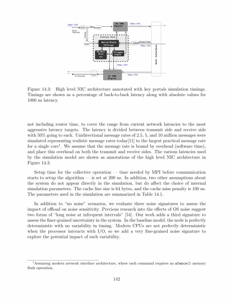
200ns / 20%

500ns / 50%

300ns / 30%

300ns / 30%

Host Interface

300ns / 30%

To Network

FromNetwork

Head

ers

Portals Cmds

FIFO FIFO

Portals Unit

FIFO

FIFO

FIFO

EngineTx DMA

Data

Offload

Atomic

Rx DMAEngine

FPU

Unit LogicTrigger

Match/Event

Figure 14.3: High level NIC architecture annotated with key portals simulation timings.Timings are shown as a percentage of back-to-back latency along with absolute values for1000 ns latency.

not including router time, to cover the range from current network latencies to the mostaggressive latency targets. The latency is divided between transmit side and receive sidewith 50% going to each. Unidirectional message rates of 2.5, 5, and 10 million messages weresimulated representing realistic message rates today[11] to the largest practical message ratefor a single core1. We assume that the message rate is bound by overhead (software time),and place this overhead on both the transmit and receive sides. The various latencies usedby the simulation model are shown as annotations of the high level NIC architecture inFigure 14.3.

Setup time for the collective operation — time needed by MPI before communicationstarts to setup the algorithm — is set at 200 ns. In addition, two other assumptions aboutthe system do not appear directly in the simulation, but do affect the choice of internalsimulation parameters. The cache line size is 64 bytes, and the cache miss penalty is 100 ns.The parameters used in the simulation are summarized in Table 14.1.

In addition to “no noise” scenarios, we evaluate three noise signatures to assess theimpact of offload on noise sensitivity. Previous research into the effects of OS noise suggesttwo forms of “long noise at infrequent intervals” [54]. Our work adds a third signature toassess the finer-grained uncertainty in the system. In the baseline model, the node is perfectlydeterministic with no variability in timing. Modern CPUs are not perfectly deterministicwhen the processor interacts with I/O, so we add a very fine-grained noise signature toexplore the potential impact of such variability.

1Assuming modern network interface architecture, where each command requires an sfence() memoryflush operation.

142

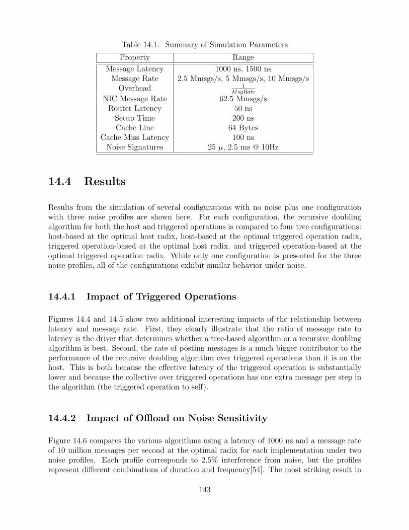
Table 14.1: Summary of Simulation Parameters

Property Range

Message Latency 1000 ns, 1500 nsMessage Rate 2.5 Mmsgs/s, 5 Mmsgs/s, 10 Mmsgs/s

Overhead 1MsgRate

NIC Message Rate 62.5 Mmsgs/sRouter Latency 50 ns

Setup Time 200 nsCache Line 64 Bytes

Cache Miss Latency 100 nsNoise Signatures 25 µ, 2.5 ms @ 10Hz

14.4 Results

Results from the simulation of several configurations with no noise plus one configurationwith three noise profiles are shown here. For each configuration, the recursive doublingalgorithm for both the host and triggered operations is compared to four tree configurations:host-based at the optimal host radix, host-based at the optimal triggered operation radix,triggered operation-based at the optimal host radix, and triggered operation-based at theoptimal triggered operation radix. While only one configuration is presented for the threenoise profiles, all of the configurations exhibit similar behavior under noise.

14.4.1 Impact of Triggered Operations

Figures 14.4 and 14.5 show two additional interesting impacts of the relationship betweenlatency and message rate. First, they clearly illustrate that the ratio of message rate tolatency is the driver that determines whether a tree-based algorithm or a recursive doublingalgorithm is best. Second, the rate of posting messages is a much bigger contributor to theperformance of the recursive doubling algorithm over triggered operations than it is on thehost. This is both because the effective latency of the triggered operation is substantiallylower and because the collective over triggered operations has one extra message per step inthe algorithm (the triggered operation to self).

14.4.2 Impact of Offload on Noise Sensitivity

Figure 14.6 compares the various algorithms using a latency of 1000 ns and a message rateof 10 million messages per second at the optimal radix for each implementation under twonoise profiles. Each profile corresponds to 2.5% interference from noise, but the profilesrepresent different combinations of duration and frequency[54]. The most striking result in

143

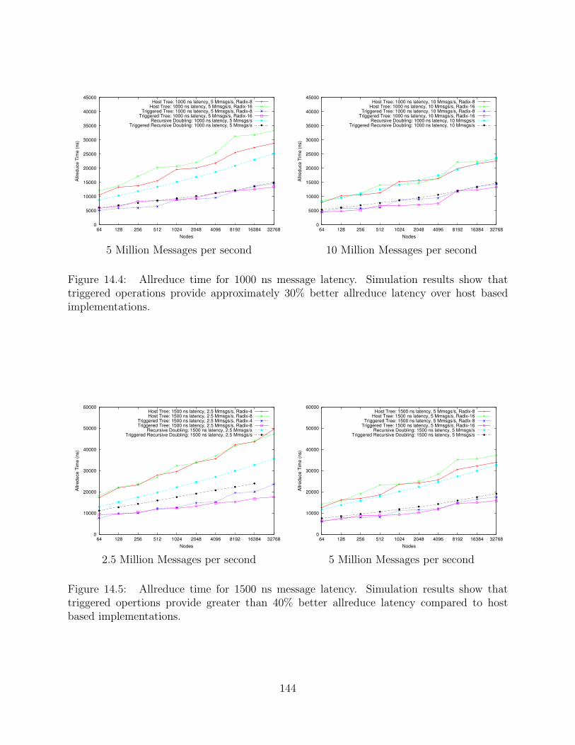
0

5000

10000

15000

20000

25000

30000

35000

40000

45000

64 128 256 512 1024 2048 4096 8192 16384 32768

Allr

educe T

ime (

ns)

Nodes

Host Tree: 1000 ns latency, 5 Mmsgs/s, Radix-8Host Tree: 1000 ns latency, 5 Mmsgs/s, Radix-16

Triggered Tree: 1000 ns latency, 5 Mmsgs/s, Radix-8Triggered Tree: 1000 ns latency, 5 Mmsgs/s, Radix-16

Recursive Doubling: 1000 ns latency, 5 Mmsgs/sTriggered Recursive Doubling: 1000 ns latency, 5 Mmsgs/s

0

5000

10000

15000

20000

25000

30000

35000

40000

45000

64 128 256 512 1024 2048 4096 8192 16384 32768

Allr

educe T

ime (

ns)

Nodes

Host Tree: 1000 ns latency, 10 Mmsgs/s, Radix-8Host Tree: 1000 ns latency, 10 Mmsgs/s, Radix-16

Triggered Tree: 1000 ns latency, 10 Mmsgs/s, Radix-8Triggered Tree: 1000 ns latency, 10 Mmsgs/s, Radix-16

Recursive Doubling: 1000 ns latency, 10 Mmsgs/sTriggered Recursive Doubling: 1000 ns latency, 10 Mmsgs/s

5 Million Messages per second 10 Million Messages per second

Figure 14.4: Allreduce time for 1000 ns message latency. Simulation results show thattriggered operations provide approximately 30% better allreduce latency over host basedimplementations.

0

10000

20000

30000

40000

50000

60000

64 128 256 512 1024 2048 4096 8192 16384 32768

Allr

educe T

ime (

ns)

Nodes

Host Tree: 1500 ns latency, 2.5 Mmsgs/s, Radix-4Host Tree: 1500 ns latency, 2.5 Mmsgs/s, Radix-8

Triggered Tree: 1500 ns latency, 2.5 Mmsgs/s, Radix-4Triggered Tree: 1500 ns latency, 2.5 Mmsgs/s, Radix-8

Recursive Doubling: 1500 ns latency, 2.5 Mmsgs/sTriggered Recursive Doubling: 1500 ns latency, 2.5 Mmsgs/s

0

10000

20000

30000

40000

50000

60000

64 128 256 512 1024 2048 4096 8192 16384 32768

Allr

educe T

ime (

ns)

Nodes

Host Tree: 1500 ns latency, 5 Mmsgs/s, Radix-8Host Tree: 1500 ns latency, 5 Mmsgs/s, Radix-16

Triggered Tree: 1500 ns latency, 5 Mmsgs/s, Radix-8Triggered Tree: 1500 ns latency, 5 Mmsgs/s, Radix-16

Recursive Doubling: 1500 ns latency, 5 Mmsgs/sTriggered Recursive Doubling: 1500 ns latency, 5 Mmsgs/s

2.5 Million Messages per second 5 Million Messages per second

Figure 14.5: Allreduce time for 1500 ns message latency. Simulation results show thattriggered opertions provide greater than 40% better allreduce latency compared to hostbased implementations.

144

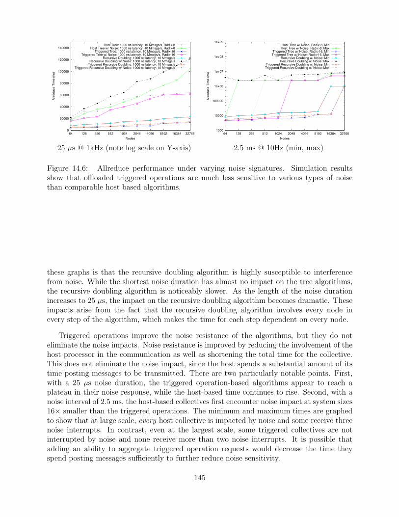
0

20000

40000

60000

80000

100000

120000

140000

64 128 256 512 1024 2048 4096 8192 16384 32768

Allr

educe T

ime (

ns)

Nodes

Host Tree: 1000 ns latency, 10 Mmsgs/s, Radix-8Host Tree w/ Noise: 1000 ns latency, 10 Mmsgs/s, Radix-8

Triggered Tree: 1000 ns latency, 10 Mmsgs/s, Radix-16Triggered Tree w/ Noise: 1000 ns latency, 10 Mmsgs/s, Radix-16

Recursive Doubling: 1000 ns latency, 10 Mmsgs/sRecursive Doubling w/ Noise: 1000 ns latency, 10 Mmsgs/s

Triggered Recursive Doubling: 1000 ns latency, 10 Mmsgs/sTriggered Recursive Doubling w/ Noise: 1000 ns latency, 10 Mmsgs/s

1000

10000

100000

1e+06

1e+07

1e+08

1e+09

64 128 256 512 1024 2048 4096 8192 16384 32768

Allr

educe T

ime (

ns)

Nodes

Host Tree w/ Noise: Radix-8, MinHost Tree w/ Noise: Radix-8, Max

Triggered Tree w/ Noise: Radix-16, MinTriggered Tree w/ Noise: Radix-16, Max

Recursive Doubling w/ Noise: MinRecursive Doubling w/ Noise: Max

Triggered Recursive Doubling w/ Noise: MinTriggered Recursive Doubling w/ Noise: Max

25 µs @ 1kHz (note log scale on Y-axis) 2.5 ms @ 10Hz (min, max)

Figure 14.6: Allreduce performance under varying noise signatures. Simulation resultsshow that offloaded triggered operations are much less sensitive to various types of noisethan comparable host based algorithms.

these graphs is that the recursive doubling algorithm is highly susceptible to interferencefrom noise. While the shortest noise duration has almost no impact on the tree algorithms,the recursive doubling algorithm is noticeably slower. As the length of the noise durationincreases to 25 µs, the impact on the recursive doubling algorithm becomes dramatic. Theseimpacts arise from the fact that the recursive doubling algorithm involves every node inevery step of the algorithm, which makes the time for each step dependent on every node.

Triggered operations improve the noise resistance of the algorithms, but they do noteliminate the noise impacts. Noise resistance is improved by reducing the involvement of thehost processor in the communication as well as shortening the total time for the collective.This does not eliminate the noise impact, since the host spends a substantial amount of itstime posting messages to be transmitted. There are two particularly notable points. First,with a 25 µs noise duration, the triggered operation-based algorithms appear to reach aplateau in their noise response, while the host-based time continues to rise. Second, with anoise interval of 2.5 ms, the host-based collectives first encounter noise impact at system sizes16× smaller than the triggered operations. The minimum and maximum times are graphedto show that at large scale, every host collective is impacted by noise and some receive threenoise interrupts. In contrast, even at the largest scale, some triggered collectives are notinterrupted by noise and none receive more than two noise interrupts. It is possible thatadding an ability to aggregate triggered operation requests would decrease the time theyspend posting messages sufficiently to further reduce noise sensitivity.

145

14.5 Conclusions

This section presents the triggered operations that were added to the Portals 4.0 API. Al-gorithms using those triggered operations were illustrated and implemented in simulation.The results highlight how changes in underlying assumptions can impact the choice of al-gorithm. Specifically, the increased operation rate that can be achieved using offload canincrease the radix of a tree algorithm and make it more competitive with recursive doublingalgorithms. The impact of noise on the collective algorithms is also striking. Recursive dou-bling is clearly more sensitive to noise, with the noise time dominating the collective timein many cases. Triggered operations are able to reduce, but not eliminate, the sensitivity ofcollective operations to OS interference.

146

Chapter 15

Application Scaling

Two application codes, representative of a broad set of application configuration strategies,provided us with a means for identifying some performance-limiting characteristics that weexpect to be issues as machine and applications scale to exascale.

CTH is implemented using a Bulk Synchronous Parallel (BSP[134]) programming modelfor regular, nearest neighbor communication. Charon solves a sparse linear system of equa-tions, sending many relatively small messages across an unstructured mesh.

As the number of processors increases to the scale of interest in this report, we find thatapplications can expect to encounter performance issues related to the computing environ-ment, system software, and algorithms. Careful profiling of runtime performance will beneeded to identify the source of the issue, in strong combination with knowledge of systemsoftware and application source code.

15.1 Boundary Exchange with Nearest Neighbors

CTH is a multi-material, large deformation, strong shock wave, solid mechanics code de-veloped at Sandia National Laboratories [66]. CTH has models for multi-phase, elasticviscoplastic, porous and explosive materials, using second-order accurate numerical methodsto reduce dispersion and dissipation and produce accurate, efficient results. Written usingthe Fortran programming language, parallelism is enabled by MPI.

Computation is characterized by regular memory accesses, and is fairly cache-friendly,with operations focusing on two dimensional planes. Inter-process communication aggregatesinternal-boundary data for all variables into user managed message buffers, subsequently sentto up to six nearest neighbors.

We begin the analysis with a case study of an important simulation at problem scales pre-viously unavailable. Experiences from this work then informs a deeper dive on performanceissues using a miniapp from the Mantevo suite, and then an additional study considering ahybrid MPI + OpenMP implementation.

147

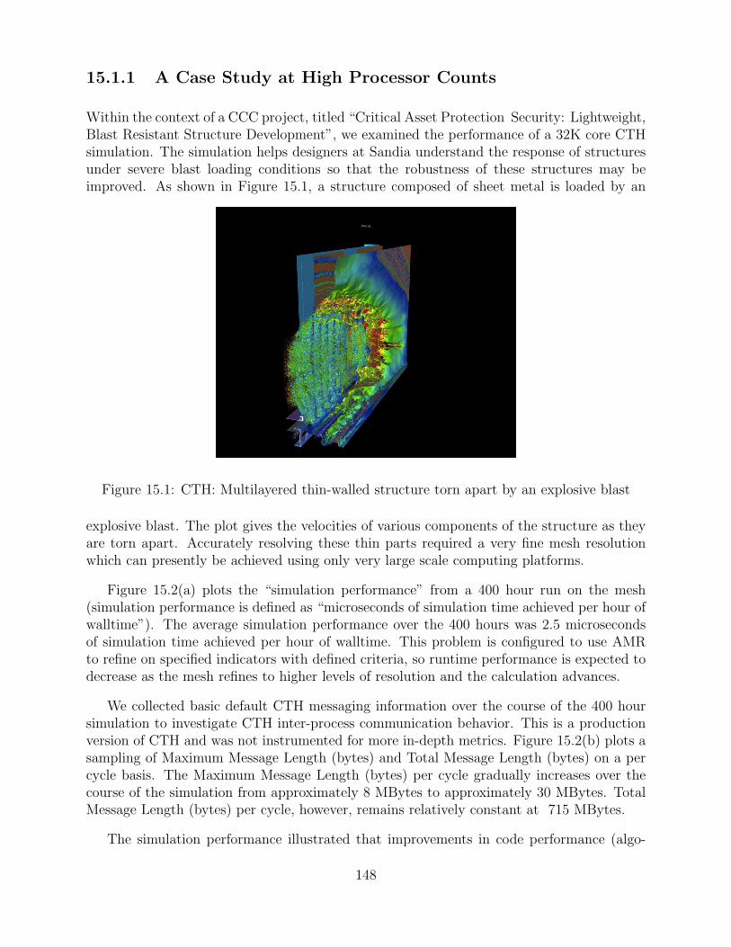
15.1.1 A Case Study at High Processor Counts

Within the context of a CCC project, titled “Critical Asset Protection Security: Lightweight,Blast Resistant Structure Development”, we examined the performance of a 32K core CTHsimulation. The simulation helps designers at Sandia understand the response of structuresunder severe blast loading conditions so that the robustness of these structures may beimproved. As shown in Figure 15.1, a structure composed of sheet metal is loaded by an

Figure 15.1: CTH: Multilayered thin-walled structure torn apart by an explosive blast

explosive blast. The plot gives the velocities of various components of the structure as theyare torn apart. Accurately resolving these thin parts required a very fine mesh resolutionwhich can presently be achieved using only very large scale computing platforms.

Figure 15.2(a) plots the “simulation performance” from a 400 hour run on the mesh(simulation performance is defined as “microseconds of simulation time achieved per hour ofwalltime”). The average simulation performance over the 400 hours was 2.5 microsecondsof simulation time achieved per hour of walltime. This problem is configured to use AMRto refine on specified indicators with defined criteria, so runtime performance is expected todecrease as the mesh refines to higher levels of resolution and the calculation advances.

We collected basic default CTH messaging information over the course of the 400 hoursimulation to investigate CTH inter-process communication behavior. This is a productionversion of CTH and was not instrumented for more in-depth metrics. Figure 15.2(b) plots asampling of Maximum Message Length (bytes) and Total Message Length (bytes) on a percycle basis. The Maximum Message Length (bytes) per cycle gradually increases over thecourse of the simulation from approximately 8 MBytes to approximately 30 MBytes. TotalMessage Length (bytes) per cycle, however, remains relatively constant at 715 MBytes.

The simulation performance illustrated that improvements in code performance (algo-

148

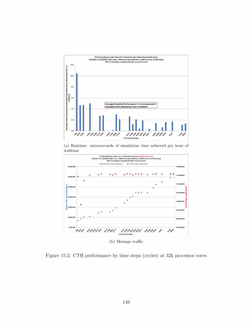
(a) Runtime: microseconds of simulation time achieved per hour ofwalltime

(b) Message traffic

Figure 15.2: CTH performance by time steps (cycles) at 32k processor cores

149

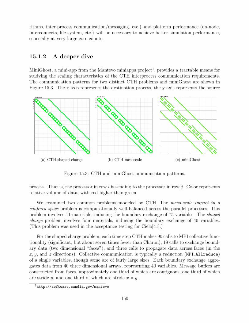
rithms, inter-process communication/messaging, etc.) and platform performance (on-node,interconnects, file system, etc.) will be necessary to achieve better simulation performance,especially at very large core counts.

15.1.2 A deeper dive

MiniGhost, a mini-app from the Mantevo miniapps project1, provides a tractable means forstudying the scaling characteristics of the CTH interprocess communication requirements.The communication patterns for two distinct CTH problems and miniGhost are shown inFigure 15.3. The x-axis represents the destination process, the y-axis represents the source

(a) CTH shaped charge (b) CTH mesoscale (c) miniGhost

Figure 15.3: CTH and miniGhost ommunication patterns.

process. That is, the processor in row i is sending to the processor in row j. Color representsrelative volume of data, with red higher than green.

We examined two common problems modeled by CTH. The meso-scale impact in aconfined space problem is computationally well-balanced across the parallel processes. Thisproblem involves 11 materials, inducing the boundary exchange of 75 variables. The shapedcharge problem involves four materials, inducing the boundary exchange of 40 variables.(This problem was used in the acceptance testing for Cielo[41].)

For the shaped charge problem, each time step CTH makes 90 calls to MPI collective func-tionality (significant, but about seven times fewer than Charon), 19 calls to exchange bound-ary data (two dimensional “faces”), and three calls to propagate data across faces (in thex, y, and z directions). Collective communication is typically a reduction (MPI Allreduce)of a single variables, though some are of fairly large sizes. Each boundary exchange aggre-gates data from 40 three dimensional arrays, representing 40 variables. Message buffers areconstructed from faces, approximately one third of which are contiguous, one third of whichare stride y, and one third of which are stride x × y.

1http://software.sandia.gov/mantevo

150

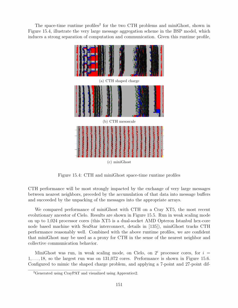
The space-time runtime profiles2 for the two CTH problems and miniGhost, shown inFigure 15.4, illustrate the very large message aggregation scheme in the BSP model, whichinduces a strong separation of computation and communication. Given this runtime profile,

(a) CTH shaped charge

(b) CTH mesoscale

(c) miniGhost

Figure 15.4: CTH and miniGhost space-time runtime profiles

CTH performance will be most strongly impacted by the exchange of very large messagesbetween nearest neighbors, preceded by the accumulation of that data into message buffersand succeeded by the unpacking of the messages into the appropriate arrays.

We compared performance of miniGhost with CTH on a Cray XT5, the most recentevolutionary ancestor of Cielo. Results are shown in Figure 15.5. Run in weak scaling modeon up to 1,024 processor cores (this XT5 is a dual-socket AMD Opteron Istanbul hex-corenode based machine with SeaStar interconnect, details in [135]), miniGhost tracks CTHperformance reasonably well. Combined with the above runtime profiles, we are confidentthat miniGhost may be used as a proxy for CTH in the sense of the nearest neighbor andcollective communication behavior.

MiniGhost was run, in weak scaling mode, on Cielo, on 2i processor cores, for i =1, . . . , 18, so the largest run was on 131,072 cores. Performance is shown in Figure 15.6.Configured to mimic the shaped charge problem, and applying a 7-point and 27-point dif-

2Generated using CrayPAT and visualized using Apprentice2.

151

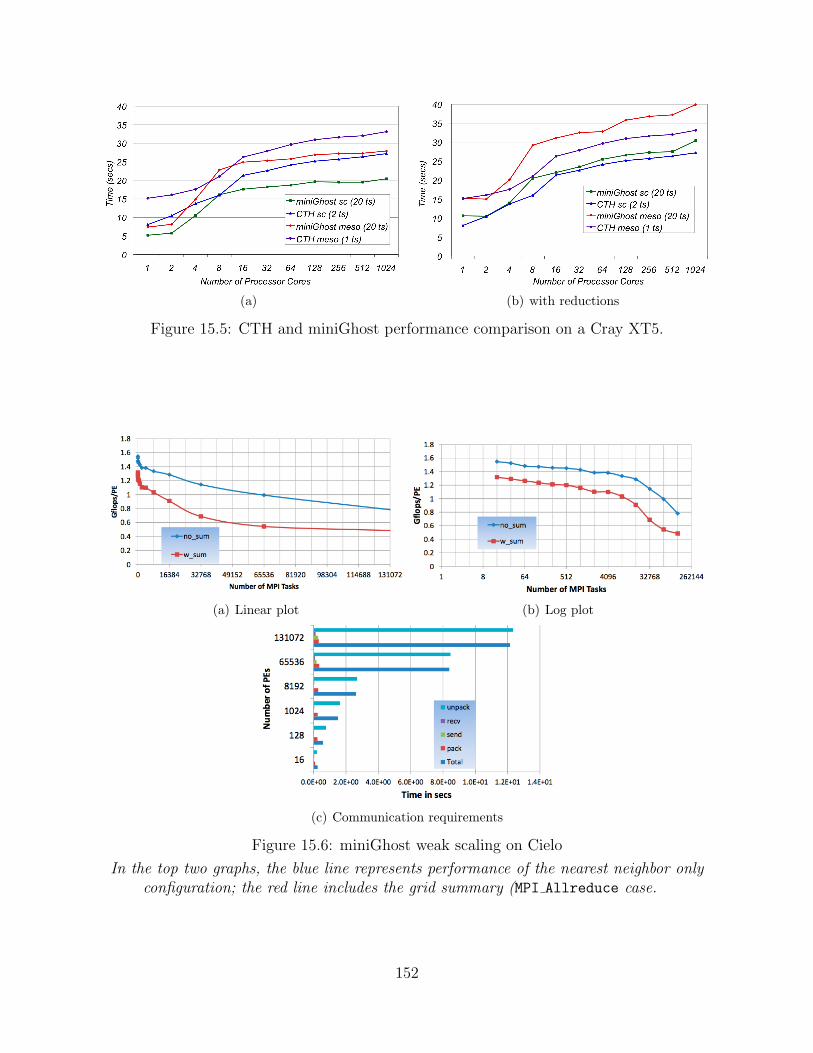
(a) (b) with reductions

Figure 15.5: CTH and miniGhost performance comparison on a Cray XT5.

(a) Linear plot (b) Log plot

(c) Communication requirements

Figure 15.6: miniGhost weak scaling on Cielo

In the top two graphs, the blue line represents performance of the nearest neighbor onlyconfiguration; the red line includes the grid summary (MPI Allreduce case.

152

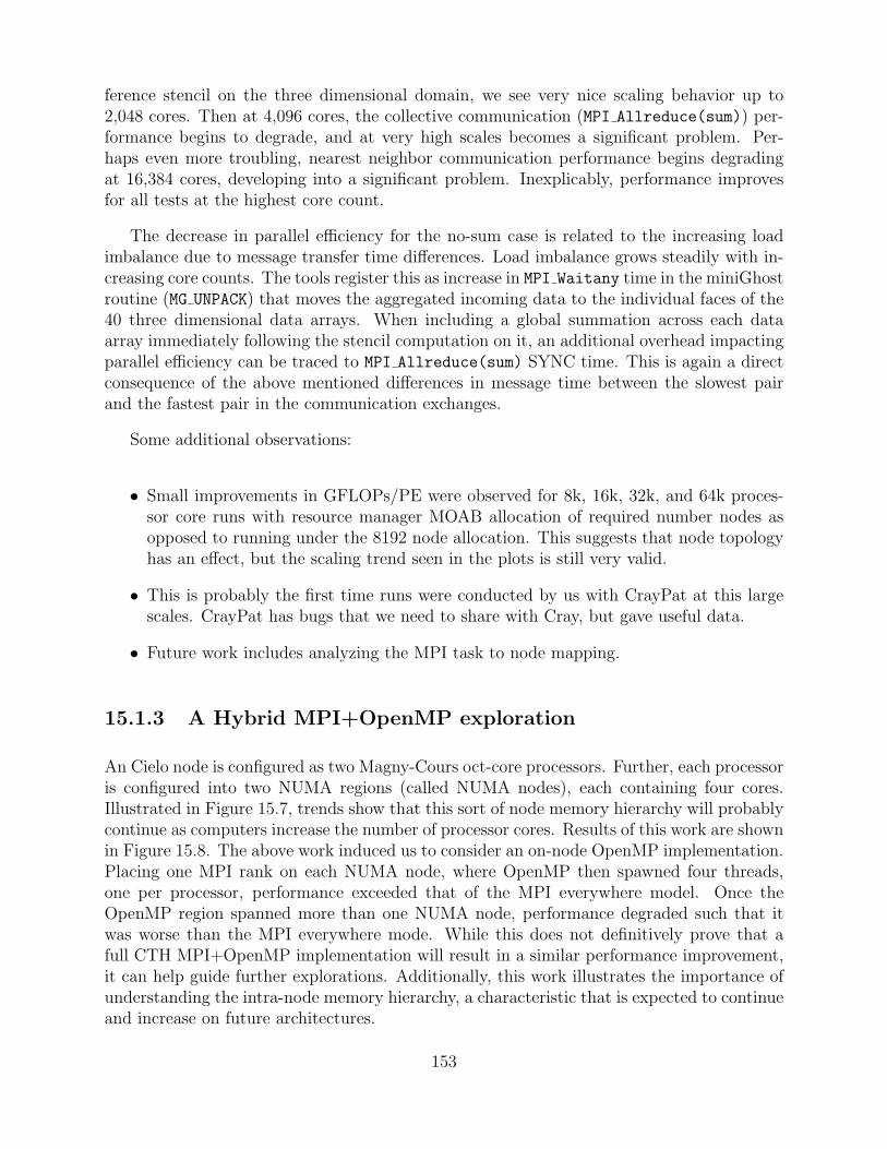
ference stencil on the three dimensional domain, we see very nice scaling behavior up to2,048 cores. Then at 4,096 cores, the collective communication (MPI Allreduce(sum)) per-formance begins to degrade, and at very high scales becomes a significant problem. Per-haps even more troubling, nearest neighbor communication performance begins degradingat 16,384 cores, developing into a significant problem. Inexplicably, performance improvesfor all tests at the highest core count.

The decrease in parallel efficiency for the no-sum case is related to the increasing loadimbalance due to message transfer time differences. Load imbalance grows steadily with in-creasing core counts. The tools register this as increase in MPI Waitany time in the miniGhostroutine (MG UNPACK) that moves the aggregated incoming data to the individual faces of the40 three dimensional data arrays. When including a global summation across each dataarray immediately following the stencil computation on it, an additional overhead impactingparallel efficiency can be traced to MPI Allreduce(sum) SYNC time. This is again a directconsequence of the above mentioned differences in message time between the slowest pairand the fastest pair in the communication exchanges.

Some additional observations:

• Small improvements in GFLOPs/PE were observed for 8k, 16k, 32k, and 64k proces-sor core runs with resource manager MOAB allocation of required number nodes asopposed to running under the 8192 node allocation. This suggests that node topologyhas an effect, but the scaling trend seen in the plots is still very valid.

• This is probably the first time runs were conducted by us with CrayPat at this largescales. CrayPat has bugs that we need to share with Cray, but gave useful data.

• Future work includes analyzing the MPI task to node mapping.

15.1.3 A Hybrid MPI+OpenMP exploration

An Cielo node is configured as two Magny-Cours oct-core processors. Further, each processoris configured into two NUMA regions (called NUMA nodes), each containing four cores.Illustrated in Figure 15.7, trends show that this sort of node memory hierarchy will probablycontinue as computers increase the number of processor cores. Results of this work are shownin Figure 15.8. The above work induced us to consider an on-node OpenMP implementation.Placing one MPI rank on each NUMA node, where OpenMP then spawned four threads,one per processor, performance exceeded that of the MPI everywhere model. Once theOpenMP region spanned more than one NUMA node, performance degraded such that itwas worse than the MPI everywhere mode. While this does not definitively prove that afull CTH MPI+OpenMP implementation will result in a similar performance improvement,it can help guide further explorations. Additionally, this work illustrates the importance ofunderstanding the intra-node memory hierarchy, a characteristic that is expected to continueand increase on future architectures.

153

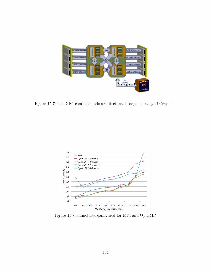
Figure 15.7: The XE6 compute node architecture. Images courtesy of Cray, Inc.

18  

19  

20  

21  

22  

23  

24  

25  

26  

27  

28  

16   32   64   128   256   512   1024   2048   4096   8192  

Time  (secon

ds)  

Number  of  processor  cores  

MPI  OpenMP,  2  threads  OpenMP,  4  threads  OpenMP,  8  threads  OpenMP,  16  threads  

Figure 15.8: miniGhost configured for MPI and OpenMP.

154

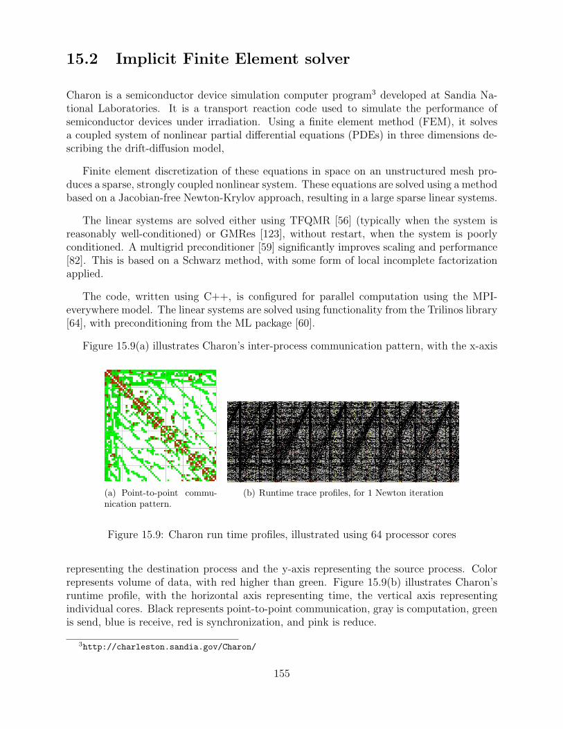
15.2 Implicit Finite Element solver

Charon is a semiconductor device simulation computer program3 developed at Sandia Na-tional Laboratories. It is a transport reaction code used to simulate the performance ofsemiconductor devices under irradiation. Using a finite element method (FEM), it solvesa coupled system of nonlinear partial differential equations (PDEs) in three dimensions de-scribing the drift-diffusion model,

Finite element discretization of these equations in space on an unstructured mesh pro-duces a sparse, strongly coupled nonlinear system. These equations are solved using a methodbased on a Jacobian-free Newton-Krylov approach, resulting in a large sparse linear systems.

The linear systems are solved either using TFQMR [56] (typically when the system isreasonably well-conditioned) or GMRes [123], without restart, when the system is poorlyconditioned. A multigrid preconditioner [59] significantly improves scaling and performance[82]. This is based on a Schwarz method, with some form of local incomplete factorizationapplied.

The code, written using C++, is configured for parallel computation using the MPI-everywhere model. The linear systems are solved using functionality from the Trilinos library[64], with preconditioning from the ML package [60].

Figure 15.9(a) illustrates Charon’s inter-process communication pattern, with the x-axis

(a) Point-to-point commu-nication pattern.

(b) Runtime trace profiles, for 1 Newton iteration

Figure 15.9: Charon run time profiles, illustrated using 64 processor cores

representing the destination process and the y-axis representing the source process. Colorrepresents volume of data, with red higher than green. Figure 15.9(b) illustrates Charon’sruntime profile, with the horizontal axis representing time, the vertical axis representingindividual cores. Black represents point-to-point communication, gray is computation, greenis send, blue is receive, red is synchronization, and pink is reduce.

3http://charleston.sandia.gov/Charon/

155

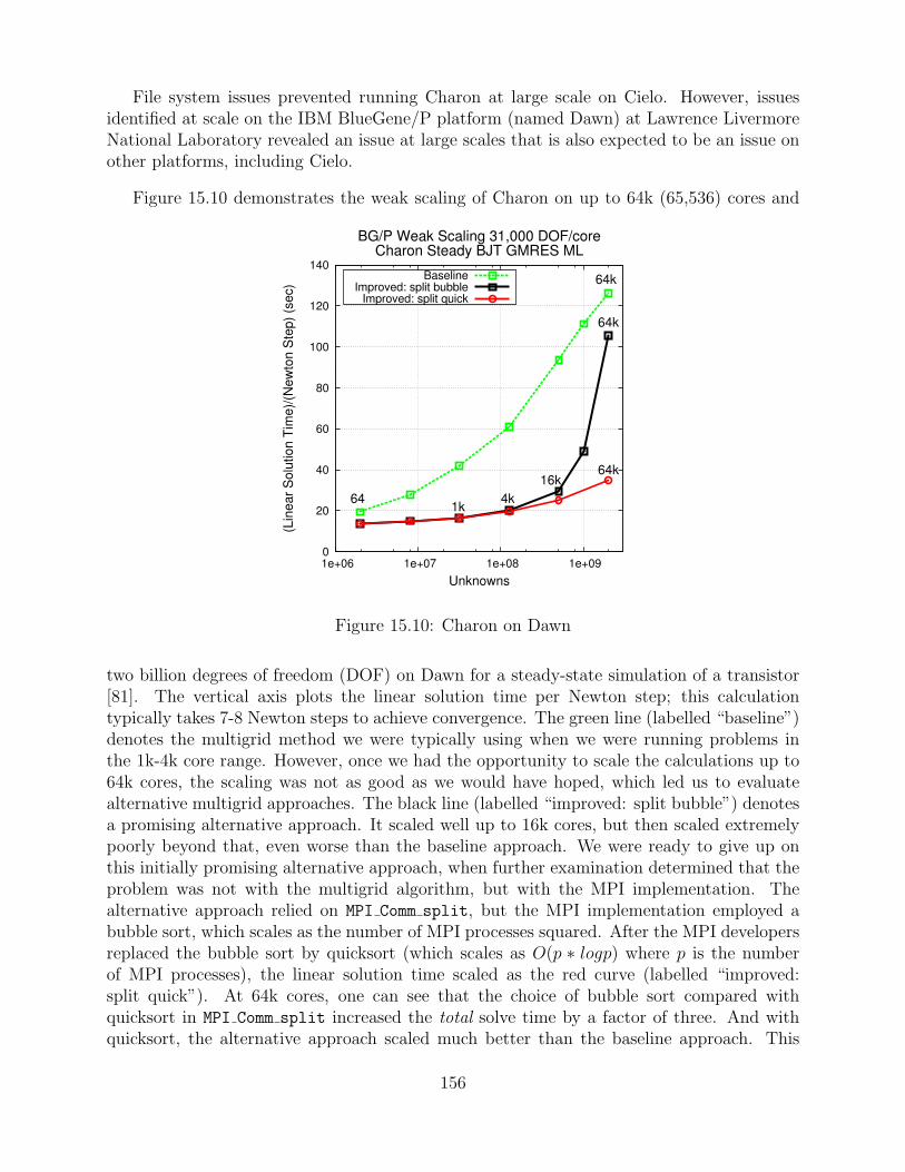
File system issues prevented running Charon at large scale on Cielo. However, issuesidentified at scale on the IBM BlueGene/P platform (named Dawn) at Lawrence LivermoreNational Laboratory revealed an issue at large scales that is also expected to be an issue onother platforms, including Cielo.

Figure 15.10 demonstrates the weak scaling of Charon on up to 64k (65,536) cores and

Figure 15.10: Charon on Dawn

two billion degrees of freedom (DOF) on Dawn for a steady-state simulation of a transistor[81]. The vertical axis plots the linear solution time per Newton step; this calculationtypically takes 7-8 Newton steps to achieve convergence. The green line (labelled “baseline”)denotes the multigrid method we were typically using when we were running problems inthe 1k-4k core range. However, once we had the opportunity to scale the calculations up to64k cores, the scaling was not as good as we would have hoped, which led us to evaluatealternative multigrid approaches. The black line (labelled “improved: split bubble”) denotesa promising alternative approach. It scaled well up to 16k cores, but then scaled extremelypoorly beyond that, even worse than the baseline approach. We were ready to give up onthis initially promising alternative approach, when further examination determined that theproblem was not with the multigrid algorithm, but with the MPI implementation. Thealternative approach relied on MPI Comm split, but the MPI implementation employed abubble sort, which scales as the number of MPI processes squared. After the MPI developersreplaced the bubble sort by quicksort (which scales as O(p ∗ logp) where p is the numberof MPI processes), the linear solution time scaled as the red curve (labelled “improved:split quick”). At 64k cores, one can see that the choice of bubble sort compared withquicksort in MPI Comm split increased the total solve time by a factor of three. And withquicksort, the alternative approach scaled much better than the baseline approach. This

156

demonstrates that a poor algorithmic choice in system libraries such as MPI can reallydestroy the performance of algorithms in an application code. Typically MPI developerswork independently of application code developers, but this example demonstrations thatmore interaction could be beneficial. Other MPI implementations such as Cray MPI werebased on the MPI implementation which used the bubble sort for MPI Comm split. So thechange to quicksort significantly improved the scaling of MPI Comm split on the Cielo CrayXE6 machine.

15.3 Conclusions and Summary

Executing application codes at significantly increased scale can result in performance degra-dation. The root cause(s) can be many and varied: hardware, system software, and algo-rithmic. Collective communication is expected to present a natural scaling issue due to theknown algorithms for supporting this functionality, and we do see this. What is somewhatunexpected is that the nearest neighbor communication exacerbates this as the number ofprocessors increases, due to the increasing probability of load imbalances induced by issuesother than the computation.

We are further investigating the use of the on-node OpenMP threading model, which forsome relatively small test cases we find may be useful for improving on-node performance.At the full application source code complexity the level of effort required to achieve thisrelatively modest performance may be prohibitive.

157

158

Chapter 16

Conclusion

The purpose of this report is to prove that the team has completed milestone 4467–Demonstrationof a Legacy Application’s Path to Exascale. As a review, we provide the milestone text below.

Cielo is expected to be the last capability system on which existing ASCcodes can run without significant modifications. This assertion will be tested todetermine where the breaking point is for an existing highly scalableapplication. The goal is to stretch the performance boundaries of theapplication by applying recent CSSE RD in areas such as resilience, power,I/O, visualization services, SMARTMAP, lightweight LWKs, virtualization, sim-ulation, and feedback loops. Dedicated system time reservations and/or CCCallocations will be used to quantify the impact of system-level changes toextend the life and performance of the ASC code base. Finally, a sim-ulation of anticipated exascale-class hardware will be performed usingSST to supplement the calculations.

The bolded text represents the actions to be completed in order to complete the milestoneitself. We will address each phrase individually.

Determine where the breaking point is for an existing highly scalable applica-tion: Chapter 15 presented the CSSE work that sought to identify the breaking point in twoASC legacy applications–Charon and CTH. Their mini-app versions were also employed tocomplete the task. There is no single breaking point as more than one issue was found withthe two codes. The results were that applications can expect to encounter performance issuesrelated to the computing environment, system software, and algorithms. Careful profiling ofruntime performance will be needed to identify the source of an issue, in strong combinationwith knowledge of system software and application source code.

Stretch the performance boundaries of the application by applying recentCSSE R&D: Chapters 2 through 14 all presented CSSE R&D work that stretched theperformance boundaries of applications. All areas enumerated in the milestone descriptionwere covered. Resilience milestone documentation is in chapter 10, power in chapter 6, I/O inchapters 7 and 13, visualization services in chapter 8, SMARTMAP in chapter 4, lightweightkernels in chapters 2, 3 and 12, virtualization is also in chapter 12, simulation in chapter 14,and finally, feedback loops in chapter 11.

159

Simulation of anticipated exascale-class hardware will be performed usingSST: Chapter 14 describes the SST simulation that was done on anticipated exascale hard-ware.

Quantify the impact of system-level changes to extend the life and perfor-mance of the ASC code base: All of the chapters quantified the impact based on metricsappropriate to the area. It is not possible to provide a single number that represents the netimprovment demonstrated by this milestone work. The measures included reduced runtime,improved job throughput, improved user productivity, and reduced power consumption. SeeTable 16.1 which lists the preformance improvement area(s) addressed by each area. Theunit of measure is different in most cases and cannot be summed. In most cases, the CSSEwork has benefit for future systems. The work provides lessons learned on what workedwell and what worked adequately. As typically happens, all efforts offer opportunities forenhancement and/or to explore new questions prompted by the work. Lastly, there is datathat was collected strickly for future co-design work and design making as we continue onour path to exascale.

160

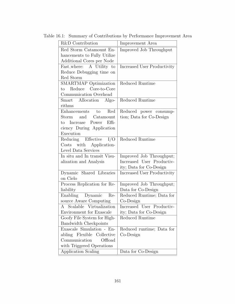
Table 16.1: Summary of Contributions by Performance Improvement Area

R&D Contribution Improvement Area

Red Storm Catamount En-hancements to Fully UtilizeAdditional Cores per Node

Improved Job Throughput

Fast where: A Utility toReduce Debugging time onRed Storm

Increased User Productivity

SMARTMAP Optimizationto Reduce Core-to-CoreCommunication Overhead

Reduced Runtime

Smart Allocation Algo-rithms

Reduced Runtime

Enhancements to RedStorm and Catamountto Increase Power Effi-ciency During ApplicationExecution

Reduced power consump-tion; Data for Co-Design

Reducing Effective I/OCosts with Application-Level Data Services

Reduced Runtime

In situ and In transit Visu-alization and Analysis

Improved Job Throughput;Increased User Productiv-ity; Data for Co-Design

Dynamic Shared Librarieson Cielo

Increased User Productivity

Process Replication for Re-liability

Improved Job Throughput;Data for Co-Design

Enabling Dynamic Re-source Aware Computing

Reduced Runtime; Data forCo-Design

A Scalable VirtualizationEnvironment for Exascale

Increased User Productiv-ity; Data for Co-Design

Goofy File System for High-Bandwidth Checkpoints

Reduced Runtime

Exascale Simulation - En-abling Flexible CollectiveCommunication Offloadwith Triggered Operations

Reduced runtime; Data forCo-Design

Application Scaling Data for Co-Design

161

162

References

[1] Mohammad H. Abbasi. Data Services: Bringing I/O Processing to Petascale. PhDthesis, Georgia Institute of Technology, May 2011.

[2] Sean Ahern, Arie Shoshani, Kwan-Liu Ma, et al. Scientific discovery at the exascale.Report from the DOE ASCR 2011 Workshop on Exascale Data Management, Analysis,and Visualization, February 2011.

[3] Jochen Alber and Rolf Niedermeier. On multi-dimensional Hilbert indexings. Theoryof Computing Systems, 1998.

[4] Carl Albing, Norm Troullier, Stephen Whalen, Ryan Olson, Howard Pritchard, JoeGlenski, and Hugo Mills. Topology, bandwidth and performance: A new approach inlinear orderings for application placement in a 3d torus. In Proceedings of the CrayUser Group Annual Technical Conference, 2011.

[5] N. Ali, P. Carns, K. Iskra, D. Kimpe, S. Lang, R. Latham, R. Ross, L. Ward, andP. Sadayappan. Scalable I/O forwarding framework for high-performance computingsystems. In Cluster Computing and Workshops, 2009. CLUSTER ’09. IEEE Interna-tional Conference on, pages 1 –10, September 2009.

[6] R. Alverson, D. Roweth, and L. Kaplan. The Gemini system interconnect. In Pro-ceedings of the 18th Annual Symposium on High Performance Interconnects (HOTI).IEEE Computer Society Press, August 2010.

[7] Saman Amarasinghe and et al. Exascale software study: Software chal-lenges in extreme scale systems. http://users.ece.gatech.edu/mrichard/

ExascaleComputingStudyReports/ECSS%20report%20101909.pdf, September 2009.

[8] Dorion C. Arnold, Dong H. Ahn, Bronis R. de Supinski, Gregory L. Lee, Barton P.Miller, and Martin Schulz. Stack trace analysis for large scale applications. In Proceed-ings of the International Parallel and Distributed Processing Symposium, Long Beach,California, March 2007.

[9] InfiniBand Trade Association. InfiniBand Architecture Specification, Release 1.2, Oc-tober 2004.

[10] James Balfour and William J. Dally. Design tradeoffs for tiled CMP on-chip networks.In Proceedings of the 20th Annual International Conference on Supercomputing, 2006.

[11] Brian W. Barrett and K. Scott Hemmert. An application based MPI message through-put benchmark. In Proceedings of the 2009 IEEE International Conference on ClusterComputing, September 2009.

163

[12] Joel F. Bartlett. A nonstop kernel. In SOSP ’81: Proceedings of the eighth ACMsymposium on Operating systems principles, pages 22–29, 1981.

[13] Sandra Johnson Baylor, Caroline Benveniste, and Yarsun Hsu. Performance evaluationof a massively parallel I/O subsystem. In Input/Output in Parallel and DistributedComputer Systems. Kluwer Academic, 1996.

[14] Michael A. Bender, David P. Bunde, Erik D. Demaine, Sandor P. Fekete, Vitus J. Le-ung, Henk Meijer, and Cynthia A. Phillips. Communication-aware processor allocationfor supercomputers: Finding point sets of small average distance. Algorithmica, 2008.

[15] John Bent, Garth Gibson, Gary Grider, Ben McClelland, Paul Nowoczynski, JamesNunez, Milo Polte, and Meghan Wingate. PLFS: A checkpoint filesystem for parallelapplications. In SC ’09 Proceedings of the Conference on High Performance ComputingNetworking, Storage and Analysis, pages 21:1–21:12, New York, NY, USA, November2009. ACM.

[16] John Bent and Gary Grider. U.S. Department of Energy best practices workshop onfile systems archives: Usability at Los Alamos National Lab. In Proceedings of the 5thDOE Workshop on HPC Best Practices: File Systems and Archives, September 2011.

[17] Keren Bergman, Shekhar Borkar, Dan Campbell, William Carlson, William Dally,Monty Denneau, Paul Franzon, William Harrod, Kerry Hill, Jon Hiller, Sher-man Karp, Stephen Keckler, Dean Klein, Peter Kogge, Robert Lucas, MarkRichards, Al Scarpelli, Steven Scott, Allan Snavely, Thomas Sterling, R. StanleyWilliams, and Katherine Yelick. Exascale computing study: Technology challengesin achieving exascale systems. http://www.science.energy.gov/ascr/Research/

CS/DARPAexascale-hardware(2008).pdf, September 2008.

[18] J. Brandt, F. Chen, V. De Sapio, A. Gentile, J. Mayo, P. Pebay, D. Roe, D. Thompson,and M. Wong. Combining Virtualization, Resource Characterization, and ResourceManagement to Enable Efficient High Performance Compute Platforms Through In-telligent Dynamic Resource Allocation. In 24th IEEE International Parallel and Dis-tributed Processing Symposium, 6th Workshop of System Management Techniques,Processes, and Services, 2010.

[19] J. Brandt, B. Debusschere, A. Gentile, J. Mayo, P. Pebay, D. Thompson, and M. Wong.OVIS-2: A Robust Distributed Architecture for Scalable RAS. In 22nd IEEE In-ternational Parallel and Distributed Processing Symposium, 4th Workshop of SystemManagement Techniques, Processes, and Services, 2008.

[20] J. Brandt, A. Gentile, D. Thompson, and T. Tucker. Develop Feedback System for In-telligent Dynamic Resource Allocation to Improve Application Performance. TechnicalReport SAND2011-6301, Sandia National Laboratories, 2011.

[21] Ron Brightwell. A prototype implementation of MPI for SMARTMAP. In Proceedingsof the 15th European PVM/MPI Users’ Group Conference, September 2008.

164

[22] Ron Brightwell, Kurt B. Ferreira, and Rolf Riesen. Transparent redundant computingwith mpi. In Rainer Keller, Edgar Gabriel, Michael M. Resch, and Jack Dongarra,editors, EuroMPI, volume 6305 of Lecture Notes in Computer Science, pages 208–218.Springer, 2010.

[23] Ron Brightwell and Kevin Pedretti. Optimizing multi-core mpi collectives withSMARTMAP. In Third International Workshop on Advanced Distributed and Par-allel Network Applications, September 2009.

[24] Ron Brightwell and Kevin Pedretti. An intra-node implementation of openshmem usingvirtual address space mapping. In Fifth Conference on Partitioned Global AddressSpace Programming Models, PGAS ’11, October 2011.

[25] Ron Brightwell, Kevin Pedretti, and Trammell Hudson. Smartmap: operating sys-tem support for efficient data sharing among processes on a multi-core processor. InProceedings of the 2008 ACM/IEEE conference on Supercomputing, SC ’08, November2008.

[26] Ron Brightwell, Kevin Pedretti, Keith Underwood, and Trammell Hudson. SeaStarinterconnect: Balanced bandwidth for scalable performance. IEEE Micro, 26(3):41–57,2006.

[27] Ron Brightwell, Rolf Riesen, Bill Lawry, and Arther B. Maccabe. Portals 3.0: protocolbuilding blocks for low overhead communication. In Proceedings of the InternationalParallel and Distributed Processing Symposium. IEEE Computer Society Press, April2002.

[28] D.M. Brooks, P. Bose, S.E. Schuster, H. Jacobson, P.N. Kudva, A. Buyuktosunoglu,J. Wellman, V. Zyuban, M. Gupta, and P.W. Cook. Power-aware microarchitecture:design and modeling challenges for next-generation microprocessors. Micro, IEEE,2000.

[29] David P. Bunde, Vitus J. Leung, and Jens Mache. Communication patterns andallocation strategies. In Proceedings of the 3rd International Workshop on PerformanceModeling, Evaluation, and Optimization of Parallel and Distributed Systems, 2004.

[30] William J. Camp and James L. Tomkins. The red storm computer architecture and itsimplementation. In The Conference on High-Speed Computing: LANL/LLNL/SNL,Salishan Lodge, Glenedon Beach, Oregon, April 2003.

[31] Franck Cappello. Fault tolerance in petascale/ exascale systems: Current knowledge,challenges and research opportunities. IJHPCA, 23(3):212–226, 2009.

[32] Miguel Castro and Barbara Liskov. Practical byzantine fault tolerance and proactiverecovery. ACM Transactions on Computer Systems (TOCS), 20(4):398–461, November2002.

165

[33] U. Catalyurek, E. Boman, K. Devine, D. Bozdag, R. Heaphy, and Riesen L.Hypergraph-based Dynamic Load Balancing for Adaptive Scientific Computations. In21st IEEE International Parallel and Distributed Processing Symposium, 2010.

[34] J. Chapin, M. Rosenblum, S. Devine, T. Lahiri, D. Teodosiu, and A. Gupta. Hive:fault containment for shared-memory multiprocessors. In SOSP ’95: Proceedings ofthe fifteenth ACM symposium on Operating systems principles, pages 12–25, New York,NY, USA, 1995. ACM.

[35] J H Chen, A Choudhary, B de Supinski, M DeVries, E R Hawkes, S Klasky, W K Liao,K L Ma, J Mellor-Crummey, N Podhorszki, R Sankaran, S Shende, and C S Yoo. Teras-cale direct numerical simulations of turbulent combustion using S3D. ComputationalScience & Discovery, 2(1):31pp, 2009.

[36] Hank Childs. Architectural challenges and solutions for petascale postprocess-ing. Journal of Physics: Conference Series, 78(012012), 2007. DOI=10.1088/1742-6596/78/1/012012.

[37] Using Cray Performance Analysis Tools. Technical Report CrayDoc S-2376-52, Cray,Inc.

[38] Workload Management and Application Placement for the Cray Linux Environment.Technical Report CrayDoc S-2496-31, Cray, Inc.

[39] J. T. Daly. A higher order estimate of the optimum checkpoint interval for restartdumps. Future Gener. Comput. Syst., 22(3):303–312, 2006.

[40] K. Devine, E. Boman, R. Heaphy, B. Henrickson, and C. Vaughan. Zoltan DataManagement Services for Parallel Dynamic Applications. In Computing in Scienceand Engineering, volume 4, pages 90–97, 2002.

[41] D. Doerfler, Mahesh Rajan, Cindy Nuss, Cornell Wright, and Thomas Spelce.Application-Driven Acceptance of Cielo, an XE6 Petascale Capability Platform. InProc. 53rd Cray User Group Meeting, 2011.

[42] S. Domino, G. Wagner, A. Luketa-Hanlin, A. Black, and J. Sutherland. Verification forMulti-Mechanics Applications. In 48th AIAA/ASME/ASCE/AHS/ASC Structures,Structural Dynamics, and Materials Conference (AIAA Paper 2007-1933), 2007.

[43] S. P. Domino, C. D. Moen, S. P. Burns, and G. H. Evans. SIERRA/Fuego A Multi-Mechanics Fire Environment Simulation Tool. In 41st AIAA Aerospace Sciences Meet-ing (AIAA Paper 2003-0149), 2003.

[44] Jr. E. S. Hertel, R. L. Bell, M. G. Elrick, A. V. Farnsworth, G. I. Kerley, J. M. McGlaun,S. V. PetneY, S. A. Silling, P. A. Taylor, and L. Yarrington. CTH: A software familyfor multi-dimensional shock physics analysis. In Proceedings of the 19th InternationalSymposium on Shock Waves, pages 377–382, July 1993.

166

[45] H. C. Edwards. Sierra Framework Version 3: Core Services Theory and Design. Tech-nical Report SAND2002-3616, Sandia National Laboratories, 2002.

[46] E. N. (Mootaz) Elnozahy, Lorenzo Alvisi, Yi-Min Wang, and David B. Johnson. Asurvey of rollback-recovery protocols in message-passing systems. ACM Comput. Surv.,34(3):375–408, 2002.

[47] E.N. Elnozahy and J.S. Plank. Checkpointing for peta-scale systems: a look intothe future of practical rollback-recovery. Dependable and Secure Computing, IEEETransactions on, 1(2):97–108, April 2004.

[48] Christian Engelmann, Hong H. Ong, and Stephen L. Scott. The case for modularredundancy in large-scale high performance computing systems. In Proceedings ofthe 8th IASTED International Conference on Parallel and Distributed Computing andNetworks (PDCN) 2009, pages 189–194, Innsbruck, Austria, February 16-18, 2009.ACTA Press, Calgary, AB, Canada.

[49] Nathan Fabian, Kenneth Moreland, David Thompson, Andrew C. Bauer, Pat Marion,Berk Geveci, Michel Rasquin, and Kenneth E. Jansen. The paraview coprocessinglibrary: A scalable, general purpose in situ visualization library. In Proceedings of theIEEE Symposium on Large-Scale Data Analysis and Visualization, 2011.

[50] Ahmad Faraj, Pitch Patarasuk, and Xin Yuan. A study of process arrival patterns forMPI collective operations. International Journal of Parallel Programming, 36(6):543–570, December 2008.

[51] Matthew S. Farmer, Anthony Skjellum, Matthew L. Curry, and H. Lee Ward. Thedesign and implementation of SSM: A single-sided message passing library based onPortals 4.0. Technical Report UABCIS-TR-2012-01242012, Department of Computerand Information Sciences, University of Alabama at Birmingham, 115A Campbell Hall,1300 University Blvd, Birmingham, Alabama 35294-1170, to appear.

[52] Xizhou Feng, Rong Ge, and Kirk W. Cameron. Power and Energy Profiling on ScientificApplications on Distributed Systems. In Proceedings of the 19th IEEE InternationalParallel and Distributed Processing Symposium IPDPS, 2005.

[53] Kurt Ferreira, Rolf Riesen, Ron Oldfield, Jon Stearley, James H. Laros III, KevinPedretti, and Ron Brightwell. rMPI: Increasing fault resiliency in a message-passingenvironment. Technical Report SAND2011-2488, Sandia National Laboratories, 2011.

[54] Kurt B. Ferreira, Patrick Bridges, and Ron Brightwell. Characterizing applicationsensitivity to OS interference using kernel-level noise injection. In SC ’08: Proceedingsof the 2008 ACM/IEEE conference on Supercomputing, pages 1–12, Piscataway, NJ,USA, 2008. IEEE Press.

[55] Kurt B. Ferreira, Jon Stearley, James H. Laros III, Ron Oldfield, Kevin T. Pedretti,Ron Brightwell, Rolf Riesen, Patrick G. Bridges, and Dorian Arnold. Evaluating theviability of process replication reliability for exascale systems. In Scott Lathrop, JimCosta, and William Kramer, editors, SC, page 44. ACM, 2011.

167

[56] Roland W. Freund. A transpose-free quasi-minimum residual algorithm for non-Hermitian linear systems. SIAM J. Sci. Comp., 14(2):470–482, 1993.

[57] Jing Fu, Ning Liu, O. Sahni, K.E. Jansen, M.S. Shephard, and C.D. Carothers. Scalableparallel I/O alternatives for massively parallel partitioned solver systems. In Interna-tional Parallel and Distributed Processing Symposium, Workshops and PhD Forum,Atlanta, GA, April 2010.

[58] F. C. Gartner. Fundamentals of fault-tolerant distributed computing in asynchronousenvironments. ACM Computing Surveys, 31(1):1–26, March 1999.

[59] Michael W. Gee, Chris M. Siefert, Jonathan J. Hu, Ray S. Tuminaro, and Marzio G.Sala. ML 5.0 Smoothed Aggregation User’s Guide. Technical Report SAND2006-2649,Sandia National Laboratories, 2006.

[60] M.W. Gee, C.M. Siefert, J.J. Hu, R.S. Tuminaro, and M.G. Sala. ML 5.0 SmoothedAggregation User’s Guide. Technical Report SAND2006-2649, Sandia National Labo-ratories, 2006.

[61] Craig Gotsman and M. Lindenbaum. On the metric properties of discrete space-fillingcurves. IEEE Transactions on Image Processing, 1996.

[62] Francois Gygi, Erik W. Draeger, Martin Schulz, Bronis R. de Supinski, John A. Gun-nels, Vernon Austel, James C. Sexton, Franz Franchetti, Stefan Kral, Christoph W.Ueberhuber, and Juergen Lorenz. Large-scale electronic structure calculations of high-Z metals on the Blue-Gene/L platform. In Proceedings of the ACM/IEEE Conferenceon Supercomputing, 2006.

[63] Thomas J. Hacker, Fabian Romero, and Christopher D. Carothers. An analysis of clus-tered failures on large supercomputing systems. J. Parallel Distrib. Comput., 69:652–665, July 2009.

[64] M. A. Heroux, R. A. Bartlett, V. E. Howle, R.J. Hoekstra, J. J. Hu, T.G. Kolda, R. B.Lehoucq, K. R. Long, R. P. Pawlowski, E.T. Phipps, A.G. Salinger, H.K. Thornquist,R. S. Tuminaro, J.M. Willenbring, A. Williams, and K. S. Stanley. An overview of theTrilinos project. ACM Transactions on Mathematical Software, 31:397–423, September2005.

[65] Michael Heroux, Roscoe Bartlett, Vicki Howle Robert Hoekstra, Jonathan Hu, TamaraKolda, Richard Lehoucq, Kevin Long, Roger Pawlowski, Eric Phipps, Andrew Salinger,Heidi Thornquist, Ray Tuminaro, James Willenbring, and Alan Williams. An overviewof the trilinos project. ACM Transactions on Mathematical Software, 31(3):397–423,2005.

[66] E.S. Hertel, Jr., R.L. Bell, M.G. Elrick, A.V. Farnsworth, G.I. Kerley, J.M. McGlaun,S.V. Petney, S.A. Silling, P.A. Taylor, and L. Yarrington. CTH: A Software Fam-ily for Multi-Dimensional Shock Physics Analysis. In Proceedings, 19th InternationalSymposium on Shock Waves, 1993.

168

[67] David Hilbert. Uber die stetige Abbildiung einer Linie auf ein Flachenstuck. Mathe-matische Annalen, 1891.

[68] Lars Holst. The general birthday problem. In Random Graphs 93: Proceedings of thesixth international seminar on Random graphs and probabilistic methods in combina-torics and computer science, pages 201–208, New York, NY, USA, 1995. John Wiley& Sons, Inc.

[69] M. Horowitz, T. Indermaur, and R. Gonzalez. Low-power digital design. In Low PowerElectronics, 1994. Digest of Technical Papers., IEEE Symposium, 1994.

[70] IOR interleaved or random HPC benchmark. http://sourceforge.net/projects/ior-sio/.

[71] Chris Johnson, Rob Ross, et al. Visualization and knowledge discovery. Report fromthe DOE/ASCR Workshop on Visual Analysis and Data Exploration at Extreme Scale,October 2007.

[72] E. S. Hertel Jr., R. L. Bell, M. G. Elrick, A. V. Farnsworth, G. I. Kerley, J. M. McGlaun,S. V. Petney, S. A. Silling, P. A. Taylor, and L. Yarrington. CTH: A software family formulti-dimensional shock physics analysis. In R. Brun and L.D. Dumitrescu, editors,Proceedings of the 19th International Symposium on Shock Physics, volume 1, pages377–382, Marseille, France, July 1993.

[73] Suzanne M. Kelly, Ruth Klundt, and James H. Laros III. Shared libraries on a capa-bility class computer. In Cray User Group Annual Technical Conference, May 2011.

[74] D. J. Kerbyson, H. J. Alme, Adolfy Hoisie, Fabrizio Petrini, H. J. Wasserman, andM. Gittings. Predictive performance and scalability modeling of a large-scale applica-tion. In Proceedings of the ACM/IEEE conference on Supercomputing, pages 37–48,2001.

[75] David Kotz. Disk-directed I/O for MIMD multiprocessors. In Hai Jin, Toni Cortes,and Rajkumar Buyya, editors, High Performance Mass Storage and Parallel I/O: Tech-nologies and Applications, chapter 35, pages 513–535. IEEE Computer Society Pressand John Wiley & Sons, 2001.

[76] S. O. Krumke, M. V. Marathe, H. Noltemeier, V. Radhakrishnan, S. S. Ravi, and D. J.Rosenkrantz. Compact location problems. Theoretical Computer Science, 1997.

[77] Leslie Lamport. Time, clocks, and the ordering of events in a distributed system.Commun. ACM, 21(7):558–565, 1978.

[78] John R. Lange, Kevin Pedretti, Peter Dinda, Patrick G. Bridges, Chang Bae, PhilipSoltero, and Alexander Merritt. Minimal-overhead virtualization of a large scale super-computer. In Proceedings of the 7th ACM SIGPLAN/SIGOPS international conferenceon virtual execution environments, VEE ’11, 2011.

169

[79] G. L. Lee, D. H. Ahn, B. R. de Supinski, J. Gyllenhaal, and P. Miller. Pynamic: thepython dynamic benchmark. In Proceedings of the IEEE 10th International Symposiumon Workload Characterization, pages 101–106, September 2007.

[80] Vitus J. Leung, Esther M. Arkin, Michael A. Bender, David Bunde, Jeanette John-ston, Alok Lal, Joseph S. B. Mitchell, Cynthia Phillips, and Steven S. Seiden. Processorallocation on Cplant: Achieving general processor locallity using one-dimensional allo-cation strategies. In Proceedings of the 4th IEEE International Conference on ClusterComputing, 2002.

[81] P. T. Lin. Improving multigrid performance for unstructured mesh drift-diffusionsimulations on 147,000 cores. submitted to the International Journal for NumericalMethods in Engineering, 2011.

[82] Paul T. Lin and John N. Shadid. Towards Large-Scale Multi-Socket, Multicore ParallelSimulations: Performance of an MPI-only Semiconductor Device Simulator. Journalof Computational Physics, 229(19), 2010.

[83] Paul T. Lin, John N. Shadid, Marzio Sala, Raymond S. Tuminaro, Gary L. Hennigan,and Robert J. Hoekstra. Performance of a parallel algebraic multilevel preconditionerfor stabilized finite element semiconductor device modeling. Journal of ComputationalPhysics, 228(17), 2009.

[84] Virginia Lo, Kurt J. Windisch, Wanqian Liu, and Bill Nitzberg. Non-contiguous pro-cessor allocation algorithms for mesh-connected multicomputers. IEEE Transactionson Parallel and Distributed Systems, 1997.

[85] Jay Lofstead, Ron Oldfield, Todd Kordenbrock, and Charles Reiss. Extending scala-bility of collective I/O through nessie and staging. In Proceedings of the 6th ParallelData Storage Workshop, November 2011.

[86] Jens Mache and Virginia Lo. The effects of dispersal on message-passing contentionin processor allocation strategies. In Proceedings of the 3rd Joint Conference on Infor-mation Sciences, Sessions on Parallel and Distributed Processing, 1997.

[87] Jens Mache, Virginia Lo, and Kurt Windisch. Minimizing message-passing contentionin fragmentation-free processor allocation. In Proceedings of the 10th IASTED Inter-national Conference on Parallel and Distributed Computing and Systems, 1997.

[88] Frank H. Mathis. A generalized birthday problem. SIAM Review, 33(2):265–270, 1991.

[89] Timothy G. Mattson and Greg Henry. An overview of the Intel TFLOPS supercom-puter. Intel Technology Journal, Q1:12, 1998.

[90] Bruce H. McCormick, Thomas A. DeFanti, and Maxine D. Brown, editors. Visualiza-tion in Scientific Computing (special issue of Computer Graphics), volume 21. ACM,1987.

170

[91] Dennis McEvoy. The architecture of tandem’s nonstop system. In ACM ’81: Proceed-ings of the ACM ’81 conference, page 245, New York, NY, USA, 1981. ACM.

[92] Adam Moody, Greg Bronevetsky, Kathryn Mohror, and Bronis R. de Supinski. Design,modeling, and evaluation of a scalable multi-level checkpointing system. In Proceedingsof the 2010 ACM/IEEE International Conference for High Performance Computing,Networking, Storage and Analysis, SC ’10, pages 1–11, Washington, DC, USA, 2010.IEEE Computer Society.

[93] Adam Moody, Juan Fernandez, Fabrizio Petrini, and Dhabaleswar K. Panda. ScalableNIC-based reduction on large-scale clusters. In Proceedings of the ACM/IEEE SC2003Conference, November 2003.

[94] Bongki Moon, H. V. Jagadish, Christos Faloutsos, and Joel H. Saltz. Analysis of theclustering properties of Hilbert space-filling curve. IEEE Transactions on Knowledgeand Data Engineering, 2001.

[95] Sherry Moore and Lionel M. Ni. The effects of network contention on processor alloca-tion strategies. In Proceedings of the 10th International Parallel Processing Symposium,1996.

[96] Jose E. Moreira, Michael Brutman, Jose Castanos, Thomas Engelsiepen, Mark Gi-ampapa, Tom Gooding, Roger Haskin, Todd Inglett, Derek Lieber, Pat McCarthy,Mike Mundy, Jeff Parker, and Brian Wallenfelt. Designing a highly-scalable operatingsystem: The blue gene/l story. In Proceedings of the ACM / IEEE SupercomputingSC’2006 conference, 2006.

[97] Kenneth Moreland, Ron Oldfield, Pat Marion, Sebastien Joudain, Norbert Podhorszki,Venkatram Vishwanath, Nathan Fabian, Ciprian Docan, Manish Parashar, MarkHereld, Michael E. Papka, and Scott Klasky. Examples of in transit visualization.In Proceedings of the PDAC 2011 : 2nd International Workshop on Petascale DataAnalytics: Challenges and Opportunities, November 2011. Submitted.

[98] Kenneth Moreland, Ron Oldfield, Pat Marion, Sabastien Jourdain, Norbert Pod-horski, Venkatram Vishwanath, Nathan Fabian, Ciprian Docan, Manish Parashar,Mark Hereld, Michael E. Papka, and Scott Klasky. Examples of in transit visualiza-tion. In Proceedings of the 2nd International Workshop on Petascale Data Analytics,2011.

[99] P. Notz, S. Subia, M. Hopkins, H. Moffat, and D. Noble. Aria 1.5 User Manual.Technical Report SAND2007-2734, Sandia National Laboratories, 2007.

[100] Ron A. Oldfield. Lightweight storage and overlay networks for fault tolerance. TechnicalReport SAND2010-0040, Sandia National Laboratories, Albuquerque, NM, January2010.

171

[101] Ron A. Oldfield, Sarala Arunagiri, Patricia J. Teller, Seetharami Seelam, Rolf Riesen,Maria Ruiz Varela, and Philip C. Roth. Modeling the impact of checkpoints on next-generation systems. In Proceedings of the 24th IEEE Conference on Mass StorageSystems and Technologies, San Diego, CA, September 2007.

[102] Ron A. Oldfield, Sarala Arunagiri, Patricia J. Teller, Seetharami Seelam, Maria RuizVarela, Rolf Riesen, and Philip C. Roth. Modeling the impact of checkpoints on next-generation systems. In MSST ’07: Proceedings of the 24th IEEE Conference on MassStorage Systems and Technologies, pages 30–46, Washington, DC, USA, 2007. IEEEComputer Society.

[103] Ron A. Oldfield, Arthur B. Maccabe, Sarala Arunagiri, Todd Kordenbrock, RolfRiesen, Lee Ward, and Patrick Widener. Lightweight I/O for scientific applications. InProceedings of the IEEE International Conference on Cluster Computing, Barcelona,Spain, September 2006.

[104] Ron A. Oldfield, Patrick Widener, Arthur B. Maccabe, Lee Ward, and Todd Ko-rdenbrock. Efficient data-movement for lightweight I/O. In Proceedings of the 2006International Workshop on High Performance I/O Techniques and Deployment of VeryLarge Scale I/O Systems, Barcelona, Spain, September 2006.

[105] Ron A. Oldfield, Andrew Wilson, George Davidson, and Craig Ulmer. Access toexternal resources using service-node proxies. In Proceedings of the Cray User GroupMeeting, Atlanta, GA, May 2009.

[106] Ron A. Oldfield, David E. Womble, and Curtis C. Ober. Efficient parallel I/O in seismicimaging. The International Journal of High Performance Computing Applications,12(3):333–344, Fall 1998.

[107] A. J. Oliner, R. K. Sahoo, J. E. Moreira, and M. Gupta. Performance implications ofperiodic checkpointing on large-scale cluster systems. In Proceedings of the 19th IEEEInternational Parallel and Distributed Processing Symposium (IPDPS’05) - Workshop18, page 299.2, 2005.

[108] Open|SpeedShop User’s Guide. Technical Report 2.0.1 Release, Open|SpeedShop,2011.

[109] Hewlett Packard. HP NonStop computing. http://h20338.www2.hp.com/

NonStopComputing/cache/76385-0-0-0-121.html.

[110] Kevin T. Pedretti, Courtenay Vaughan, Karl Scott Hemmert, and Brian Barrett. Ap-plication sensitivity to link and injection bandwidth on a Cray XT4 system. In Pro-ceedings of the 2005 Cray User Group Annual Technical Conference, Helsinki, Finland,May 2008.

[111] Tom Peterka, Hongfeng Yu, Robert Ross, and Kwan-Liu Ma. Parallel volume render-ing on the IBM Blue Gene/P. In Proceedings of Eurographics Parallel Graphics andVisualization Symposium 2008, 2008.

172

[112] Tom Peterka, Hongfeng Yu, Robert Ross, Kwan-Liu Ma, and Rob Latham. End-to-endstudy of parallel volume rendering on the IBM Blue Gene/P. In Proceedings of ICPP’09, pages 566–573, September 2009. DOI=10.1109/ICPP.2009.27.

[113] Fabrizio Petrini, Darren Kerbyson, and Scott Pakin. The Case of the Missing Super-computer Performance: Achieving Optimal Performance on the 8,192 Processors ofASCI Q. In Proceedings of SC, 2003.

[114] Fabrizio Petrini, Darren J. Kerbyson, and Scott Pakin. The case of the missing su-percomputer performance: Identifying and eliminating the performance variability onthe ASCI Q machine. In Proceedings of the 2003 Conference on High PerformanceNetworking and Computing, November 2003.

[115] Steve J. Plimpton. Fast parallel algorithms for short-range molecular dynamics. JComp Phys, 117(1):1–19, 1995.

[116] Rolf Rabenseifner. Optimization of collective reduction operations. In ComputationalScience - ICCS 2004, 2004.

[117] Mahesh Rajan, Courtenay T. Vaughan, Doug W. Doerfler, Richard F. Barrett, Paul T.Lin, Kevin T. Pedretti, and K. Scott Hemmert. Application-drivern analysis of twogenerations of capability computing platforms: The transition to multicore processors.Concurrency and Computation: Practice and Experience, to appear, to appear.

[118] Charles Reiss, Gerald Lofstead, and Ron Oldfield. Implementation and evaluation ofa staging proxy for checkpoint I/O. Technical report, Sandia National Laboratories,Albuquerque, NM, August 2008.

[119] Rolf Riesen, Ron Brightwell, Patrick Bridges, Trammell Hudson, Arthur Maccabe,Patrick Widener, and Kurt Ferreira. Designing and implementing lightweight kernelsfor capability computing. Concurrency and Computation: Practice and Experience,21(6):793–817, August 2008.

[120] Rolf Riesen, Ron Brightwell, Kevin Pedretti, Brian Barrett, Keith Underwood,Arthur B. Maccabe, and Trammell Hudson. The Portals 4.0 message passing interface.Technical Report SAND2008-2639, Sandia National Laboratories, Albuquerque, NewMexico 87185 and Livermore, California 94550, April 2008.

[121] Rolf E. Riesen, Kevin T. Pedretti, Ron Brightwell, Brian W. Barrett, Keith D. Un-derwood, Trammell B. Hudson, and Arthur B. Maccabe. The Portals 4.0 messagepassing interface. Technical Report SAND2008-2639, Sandia National Laboratories,April 2008.

[122] R B Ross, T Peterka, H-W Shen, Y Hong, K-L Ma, H Yu, and K Moreland. Visu-alization and parallel I/O at extreme scale. Journal of Physics: Conference Series,125(012099), 2008. DOI=10.1088/1742-6596/125/1/012099.

[123] Yousef Saad and Martin H. Schultz. GMRes: a generalized minimal residual algorithmfor solving nonsymmetric linear systems. SIAM J. Sci. Stat. Comput., 7:856–869, 1986.

173

[124] Sandia National Laboratory. LAMMPS molecular dynamics simulator. http://

lammps.sandia.gov, Apr. 10 2010.

[125] Sandia National Laboratory. Mantevo project home page. https://software.

sandia.gov/mantevo, Apr. 10 2010.

[126] F. Schneider. Implementing fault-tolerant services using the state machine approach:A tutorial. ACM Computing Surveys, 22(4):299–319, 1990.

[127] Bianca Schroeder and Garth A. Gibson. A large-scale study of failures in high-performance computing systems. In Proceedings of the International Conference onDependable Systems and Networks (DSN2006), June 2006.

[128] Bianca Schroeder and Garth A Gibson. Understanding failures in petascale computers.Journal of Physics: Conference Series, 78(1):012022, 2007.

[129] M. Schulz, A. Arowojolu, J. Blanchard, J. Brandt., S. Futral, J. Mellor-Crummey,B. Miller, D. Montoya, M. Rajan, K. Roche, and Zosel. M. Tools and tool support forthe exascale era from the nnsa workshop of exascale computing technologies. LLNL-TR-472494, 2011.

[130] K. E. Seamons, Y. Chen, P. Jones, J. Jozwiak, and M. Winslett. Server-directed col-lective I/O in Panda. In Proceedings ofSupercomputing ’95, San Diego, CA, December1995. IEEE Computer Society Press.

[131] Ion Stoica, Robert Morris, David Karger, M. Frans Kaashoek, and Hari Balakrishnan.Chord: A scalable peer-to-peer lookup service for internet applications. SIGCOMMComput. Commun. Rev., 31:149–160, August 2001.

[132] K. Uhlemann, C. Engelmann, and S.L. Scott. JOSHUA: Symmetric active/activereplication for highly available hpc job and resource management. In Proceedings ofthe 2006 IEEE International Conference on Cluster Computing, Los Alamitos, CA,USA, 2006. IEEE Computer Society.

[133] Keith D. Underwood, Michael Levenhagen, and Arun Rodrigues. Simulating RedStorm: Challenges and successes in building a system simulation. In 21st InternationalParallel and Distributed Processing Symposium (IPDPS’07), March 2007.

[134] Leslie G. Valiant. A Bridging Model for Parallel Computation. Commun. ACM,33:103–111, August 1990.

[135] C.T. Vaughan, M. Rajan, R.F. Barrett, D.W. Doerfler, and K.T. Pedretti. Investigat-ing the Impact of the Cielo Cray XE6 Architecture on Scientific Application Codes.In Workshop on Large Scale Parallel Processing, at the IEEE International Parallel &Distributed Processing Symposium (IPDPS) Meeting, 2011. SAND 2010-8925C.

[136] Adam Wagner, Darius Buntinas, Ron Brightwell, and Dhabaleswar K. Panda.Application-bypass reduction for large-scale clusters. In Proceedings 2003 IEEE Con-ference on Cluster Computing, December 2003.

174

[137] Peter Walker, David P. Bunde, and Vitus J. Leung. Faster high-quality processor allo-cation. In Proceedings of the 11th LCI International Conference on High-PerformanceClustered Computing, 2010.

[138] Deborah Weisser, Nick Nystrom, Chad Vizino, Shawn T. Brown, and John Urbanic.Optimizing job placement on the Cray XT3. In Proceedings of the Cray User GroupAnnual Technical Conference, 2006.

[139] Fang Zheng, Hasan Abbasi, Ciprian Docan, Jay Lofstead, Scott Klasky, Qing Liu,Manish Parashar, Norbert Podhorszki, Karsten Schwan, and Matthew Wolf. PreDatA -preparatory data analytics on Peta-Scale machines. In Proceedings of the InternationalParallel and Distributed Processing Symposium, pages 1–12, April 2010.

[140] Ziming Zheng and Zhiling Lan. Reliability-aware scalability models for high perfor-mance computing,. In Cluster’09: Proceedings of the IEEE conference on ClusterComputing, 2009.

175

DISTRIBUTION:

MS ,

,

1 MS 0899 RIM-Reports Management, 9532 (electronic copy)

176

v1.28