RESEARCH ON TRANSFER ALIGNMENT FOR INCREASED

RESEARCH ON TRANSFER ALIGNMENT

FOR

INCREASED SPEED AND ACCURACY

A THESIS SUBMITTED TO

THE GRADUATE SCHOOL OF NATURAL AND APPLIED SCIENCES

OF

THE MIDDLE EAST TECHNICAL UNIVERSITY

BY

UĞUR KAYASAL

IN PARTIAL FULFILLMENT OF THE REQUIREMENTS

FOR

THE DEGREE OF DOCTOR OF PHILOSOPHY

IN

MECHANICAL ENGINEERING

SEPTEMBER 2012

Approval of the thesis:

RESEARCH ON TRANSFER ALIGNMENT

FOR INCREASED SPEED AND ACCURACY

Submitted by UĞUR KAYASAL in partial fulfillment of the requirements for the

degree of Doctor of Philosophy in Mechanical Engineering Department,

Middle East Technical University by,

Prof. Dr. Canan ÖZGEN _________________

Dean, Graduate School of Natural and Applied Sciences

Prof. Dr. Süha ORAL _________________

Head of the Department, Mechanical Engineering

Prof. Dr. M. Kemal ÖZGÖREN _________________

Supervisor, Mechanical Engineering Dept., METU

Examining Committee Members

Prof. Dr. Tuna BALKAN _________________

Mechanical Engineering Dept., METU

Prof. Dr. M. Kemal ÖZGÖREN _________________


Prof. Dr. Ozan TEKĠNALP _________________

Aerospace Engineering Dept., METU

Asst. Prof. Dr. E. Ġlhan KONUKSEVEN _________________


Prof. Dr. Yücel ERCAN _________________

Mechanical Engineering Dept., TOBB-ETU

Date: _________

iii

I hereby declare that all information in this document has been obtained and

presented in accordance with academic rules and ethical conduct. I also

declare that, as required by these rules and conduct, I have fully cited and

referenced all material and results that are not original to this work.

Name, Last name : UĞUR KAYASAL

Signature :

iv

ABSTRACT

RESEARCH ON TRANSFER ALIGNMENT FOR INCREASED SPEED

AND ACCURACY

KAYASAL, UĞUR

PhD., Department of Mechanical Engineering

Supervisor: Prof. Dr. M. Kemal ÖZGÖREN

September 2012, 206 pages

In this thesis, rapid transfer alignment algorithm for a helicopter launched guided

munition is studied.

Transfer alignment is the process of initialization of a guided munition’s inertial

navigation system with the aid of the carrier platform’s navigation system, which

is generally done by comparing the navigation data of missile and carrier’s

navigation data. In the literature, there are different studies of transfer alignment,

especially for aircraft launched munitions.

One important problem in transfer alignment is the attitude uncertainty of lever

arm between munition’s and carrier’s navigation systems. In order to overcome

this problem, most of the studies in the literature do not use carrier’s attitude data

in the transfer alignment, only velocity data is used. In order to estimate attitude

v

and related inertial sensor errors, specific maneuvers of carrier platform are

required which can take 1-5 minutes.

Especially for helicopter launched munitions, the transfer alignment should be

completed in limited time duration. In order to have a rapid transfer alignment,

attitude data should be included in transfer alignment with proper handling of

lever arm uncertainty. Also, mechanical vibration of helicopter is another

important problem compared to the aircraft launched systems. In aircrafts, lever

arm uncertainty due to wing flexure is the main problem, whereas both lever arm

uncertainty due to rotor based vibration and flexibility are the source of error. The

helicopter’s mechanical vibration results in another problem; performance of

MEMS based inertial sensors degrade with the presence of vibration. Modeling

and compensation of vibration induced inertial sensor errors should also be done

in a helicopter based transfer alignment

The purpose of this thesis is to compensate the errors arising from the dynamics of

the Helicopter, lever arm, mechanical vibration effects and inertial sensor error

amplification, thus designing a transfer alignment algorithm under real

environment conditions. The algorithm design begins with observability analysis,

which is not done for helicopter transfer alignment in literature. In order to make

proper compensations, characterization and modeling of vibration and lever arm

environment is done for the helicopter. Also, vibration based errors of MEMS

based inertial sensors are experimentally shown. The developed transfer

alignment algorithm is tested by simulated and experimental data

Keywords: Inertial Navigation Systems, Rapid Transfer Alignment,

Observability Analysis

vi

ÖZ

YÖNELİM AKTARIMI’NIN HIZININ VE HASSASIYETININ

ARTTIRILMASI ICIN ARASTIRMA

KAYASAL, Uğur

Doktora, Makina Mühendisliği Bölümü

Tez Yöneticisi: Prof. Dr. M. Kemal ÖZGÖREN

Ağustos 2012, 206 sayfa

Bu tezde, helikopterden fırlatılan bir güdümlü mühimmatın hızlı yönelim aktarımı

üzerine çalıĢılmıĢtır.

Yönelim aktarımı, güdümlü mühimmatın ataletsel seyrüsefer sisteminin, taĢıyıcı

platformun seyrüsefer sistemi verileri yardımıyla, genellikle her iki Navigasyon

sisteminin verilerinin karĢılaĢtırılmasıyla baĢlatılması iĢlemidir. Literatürde

özellikle uçaktan fırlatılan mühimmatlar için birçok yönelim aktarımı çalıĢması

yer almaktadır.

Yönelim aktarımındaki önemli bir sorun, mühimmat ve platform Navigasyon

sistemleri arasındaki yönelim belirsizliğidir. Bu sorunu aĢabilmek için, yönelim

aktarımında sadece platformun hız verisi kullanılırken yönelim bilgisi

vii

kullanılmaz. Yönelim ve ilgili ataletsel sensör hatalarının kestirimi için,

platformun 1-5 dakika arası süren özel manevralar yapması gerekmektedir.

Özellikle helikopterden fırlatılan mühimmatlar için yönelim aktarımı kısıtlı bir

süre içerisinde tamamlanmalıdır. Hızlı bir yönelim aktarımı yapabilmek için,

yönelim bilgisinin moment kolu belirsizliğinin uygun biçimde ele alınmasıyla

yönelim aktarımına dahil edilmesi gerekmektedir. Ayrıca, helikopterin mekanik

titreĢimi de uçaktan fırlatılan mühimmatlara göre önemli bir sorundur. Uçaklarda

esas sorun kanat esnemesinden dolayı kaynaklanan moment kolu belirsizliği iken,

helikopterler rotor kaynaklı titreĢim ve esneme esas sorun kaynaklarıdır.

Helikopterin mekanik titreĢimi bir diğer soruna daha yol açmaktadır; MEMS

tabanlı ataletsel sensörlerin performansı titreĢim altında düĢmektedir.

Helikopter’de yapılan yönelim aktarımında, titreĢime bağlı ataletsel sensör

hatalarının da karakterize edilmesi ve modellenmesi gerekmektedir.

Bu tezin amacı, Helikopter dinamiğinden kaynaklanan moment kolu, titreĢim ve

ataletsel sensör hata artmasının telafisinin yapılarak gerçek çevresel ortamda

çalıĢabilen bir yönelim aktarımı algoritması elde etmektir. Algoritmanın tasarımı,

literatürde daha önce yapılmamıĢ olan, helikopter yönelim aktarımı için

gözlenebilirlik analizi yapılarak baĢlamaktadır. Gerekli hata telafilerinin

yapılabilmesi için moment kolu ve titreĢim etkilerinin karakterizasyonu ve

modellemesi yapılmıĢtır. Ayrıca, MEMS tabanlı ataletsel sensörlerin titreĢime

bağlı hataları deneysel olarak belirlenmiĢtir. GeliĢtirilen yönelim aktarımı

algoritması, benzetim ve deneysel verilerle test edilmiĢtir.

Anahtar Kelimeler: Ataletsel Seyrüsefer Sistemi, Hızlı Yönelim Aktarımı,

Gözlenebilirlik Analizi

viii

To my family…

ix

ACKNOWLEDGMENTS

I would like to express my gratitude to my supervisor Prof. Dr. M.Kemal Özgören

for his never ending guidance, patience, advice, understanding, and support

throughout my research.

I also would like to thank my Thesis Examining Committee members Prof.Dr.

Ozan Tekinalp and Asst.Prof.Dr. Ġlhan Konukseven for their comments.

I am grateful to my colleagues in Roketsan for their invaluable comments and

suggestions.

Dr. Sartuk Karasoy and Mr. Bülent Semerci are kindly acknowledged for their

support in this thesis.

I would like to thank all members of my family for their guidance, encouragement

and support.

Finally, I would like to thank to my wife Esen and my daughter Özge for their

everlasting support, patience and love. Without their support, this work could not

be completed.

x

TABLE OF CONTENTS

ABSTRACT ........................................................................................................... iv

ÖZ ........................................................................................................................ vi

ACKNOWLEDGMENTS ...................................................................................... ix

TABLE of CONTENTS .......................................................................................... x

LIST OF SYMBOLS AND ABBREVIATIONS ................................................. xiii

LIST OF FIGURES .............................................................................................. xvi

CHAPTERS

1 INTRODUCTION ........................................................................................... 1

1.1 Motivation ............................................................................................... 1

1.2 Literature Survey and Current Applications ........................................... 6

1.3 Drawbacks of the Current Applications ................................................ 14

1.4 Objectives of the Thesis ........................................................................ 14

1.5 Outline of the Thesis ............................................................................. 18

2 STRAPDOWN INERTIAL NAVIGATION SYSTEMS ............................. 19

2.1 Inertial Measurement Unit ..................................................................... 19

2.1.1 IMU Technologies ......................................................................... 20

2.1.2 Error Model of IMU ...................................................................... 22

2.2 Inertial Navigation System .................................................................... 25

2.2.1 Inertial Navigation Mechanization Equations ............................... 26

2.2.1.1 Coordinate Frames ................................................................ 26

2.2.1.1.1 Inertial Frame ....................................................................... 26

2.2.1.1.2 Earth frame .......................................................................... 27

2.2.1.1.3 Navigation frame ................................................................. 27

2.2.1.2 Coordinate Transformation Between Reference Frames ...... 27

2.2.1.3 Earth Model ........................................................................... 28

2.2.1.4 Gravity Model ....................................................................... 28

2.2.1.5 Inertial Navigation Kinematic Equations .............................. 29

xi

2.2.2 Error Model of Inertial Navigation Systems ................................. 30

3 RAPID TRANSFER ALIGNMENT ............................................................ 32

3.1 Rapid Transfer Alignment Algorithm ................................................... 32

3.1.1 Measurement ................................................................................. 35

3.1.2 Estimation ...................................................................................... 36

3.1.3 Feedback ........................................................................................ 37

4 OBSERVABILITY ANALYSIS ................................................................. 38

4.1 Observability Analysis Methods ........................................................... 40

4.1.1 Eigen Value Approach .................................................................. 41

4.1.2 Covariance Matrix Approach ........................................................ 45

4.2 Observability Analysis of Transfer Alignment Maneuvers .................. 47

5 VIBRATION DEPENDENT INERTIAL SENSOR ERRORS .................... 62

5.1 Effects of Vibration on Transfer Alignment Performance .................... 64

5.2 Characterization of Vibration Environment .......................................... 70

5.3 Characterization of Vibration Dependent Errors ................................... 75

6 FLEXIBLE LEVER ARM IN TRANSFER

ALIGNMENT ....................................................................................................... 82

6.1 Characterization of Flexible Lever Arm ............................................... 82

6.2 Error Modeling Approaches .................................................................. 95

6.2.1 State Augmentation ....................................................................... 97

6.2.2 Artificial Neural Network ........................................................... 104

6.2.3 Comparison of Methods .............................................................. 107

7 IMPROVED RAPID TRANSFER ALIGNMENT ..................................... 127

7.1 Improvements in Transfer Alignment ................................................. 127

7.2 Rapid Transfer Alignment Simulation Results ................................... 128

7.2.1 Simulation with Vibration Effects ............................................... 129

7.2.2 Simulation with Flexibility Effects ............................................. 136

7.3 Rapid Transfer Alignment Experimental Results ............................... 141

8 DISCUSSION and CONCLUSION ............................................................ 151

A DERIVATION OF INS EQUATIONS ........................................ 164

B DERIVATION OF INS ERROR EQUATIONS ........................................ 169

B.1 Attitude Errors ................................................................................ 169

xii

B.2 Velocity Errors ............................................................................... 172

B.3 Position Errors ................................................................................ 173

C ARTIFICIAL NEURAL NETWORKS ...................................................... 176

D KALMAN FILTERING ............................................................................. 183

E INERTIAL SENSOR SPECIFICATIONS ................................................. 188

F SIMULINK MODELS FOR RAPID TRANSFER ALIGNMENT ............ 190

F.1 INPUT FILE FOR ALGORITHM ................................................. 190

F.2 SIMULINK BLOCKS ................................................................... 199

CURRICULUM VITAE ................................................................................ 204

xiii

LIST OF SYMBOLS AND ABBREVIATIONS

Symbol

Definition

i Inertial frame

b Body frame

n Navigation frame

n

bC Direction cosine matrix between navigation and body

frame

Roll attitude

Pitch attitude

Azimuth attitude

w Angular rates

a Linear acceleration

xS Scale factor error in x axis

xym Misalignment error between x and y axis

b

ib Angular rate between inertial and body frame, defined

in body frame

n

in Error in angular rates between inertial and navigation

frame, defined in navigation frame

n

bC Direction cosine matrix Error

n Misalignment vector defining the error in DCM

Magnitude of Earth rotation rate

R The length of semi major axis

r The length of semi minor axis

xiv

f The flattening of semi minor axis

e The major eccentricity

L Latitude

l Longitude

h Altitude

g Gravity vector

V Velocity

Position errors

kx State vector

kz Measurement vector

kA System matrix

kH Measurement matrix

kw Process Noise vector

kv Measurement Noise vector

kP State Covariance Matrix

kQ Process Noise covariance matrix

kR Measurement Noise covariance matrix

kK Kalman Gain

w Cross product matrix form

State Transition matrix

Q Observability matrix

,

n

b slaveC Slave DCM

,

n

b masterC

Master DCM

master

slaveC

Master to Slave DCM

C(m,k) Penalty function

(k) Error Probability

m Sample Size

k Order of Markov Process

xv

Abbreviation Definition

INS Inertial Navigation System

IMU Inertial Measurement Unit

GNSS Global Navigation Satellite System

FOG Fiber Optic Gyro

RLG Ring Laser Gyro

MEMS Micro Electro Mechanical System

RMS Root Mean Square

ANN Artificial Neural Network

Throughout the text,

Numbers in brackets DENOTE

References

Numbers in parenthesis Equations

2 Innovation variance

Estimated innovation

Rt Autocorrelation

xvi

LIST OF FIGURES

Figures

Figure 2.1 Inertial Sensor Error Characteristics [13] ............................................ 24

Figure 3.1 Rapid Transfer Alignment Algorithm Flow ........................................ 33

Figure 3.2 Direct Kalman Filter ............................................................................ 34

Figure 3.3 Indirect Feedforward Kalman Filter .................................................... 34

Figure 3.4 Indirect Feedback Kalman Filter ......................................................... 35

Figure 4.1 Sample Observability for Hover case, Eigenvalue Approach ............. 44

Figure 4.2 Sample Observability for Hover case, Z Domain ................................ 44

Figure 4.3 Sample Observability for Hover case, Covariance Matrix Approach . 46

Figure 4.4 Observability for Hover, Analyzed by Method 1, Accelerometer Errors

............................................................................................................................... 48

Figure 4.5 Observability for Hover, Analyzed by Method 1, Gyro Errors ........... 48

Figure 4.6 Observability for Hover, Analyzed by Method 1, Navigation Errors .. 49


............................................................................................................................... 49

Figure 4.8 Observability for Hover, Analyzed by Method 2, Gyro Errors ........... 50

Figure 4.9 Observability for Hover, Analyzed by Method 2, Navigation Errors .. 50

Figure 4.10 Observability for Straight Flight with Longitudinal Acceleration,

Analyzed by Method 1, Accelerometer Errors ...................................................... 51


Analyzed by Method 1, Gyro Errors ..................................................................... 52


Analyzed by Method 1, Navigation Errors ........................................................... 52


Analyzed by Method 2, Accelerometer Errors ...................................................... 53


Analyzed by Method 2, Gyro Errors ..................................................................... 53

xvii


Analyzed by Method 2, Navigation Errors ........................................................... 54

Figure 4.16 Observability for Level Sinusoidal Flight, Analyzed by Method 1,

Accelerometer Errors ............................................................................................ 55


Gyro Errors ............................................................................................................ 55


Navigation Errors .................................................................................................. 56




Gyro Errors ............................................................................................................ 57



Figure 4.22 Observability for Sinusoidal Flight with Roll, Analyzed by Method 1,



Gyro Errors ............................................................................................................ 58






Gyro Errors ............................................................................................................ 60



Figure 5.1 Vibration Profile for Environmental Tests [50] ................................... 64

Figure 5.2 Vibration Profile measured in the test equipment ................................ 66

Figure 5.3 X Accelerometer Bias Estimation with Random Vibration ................. 67

Figure 5.4 Y Accelerometer Bias Estimation with Random Vibration ................. 68

Figure 5.5 Z Accelerometer Bias Estimation with Random Vibration ................. 68

Figure 5.6 X Gyro Bias Estimation with Different Vibration Amplitudes ........... 69

xviii

Figure 5.7 Y Gyro Bias Estimation with Random Vibration ................................ 69

Figure 5.8 Z Gyro Bias Estimation with Random Vibration ................................ 70

Figure 5.9 Vibration Profile for Hover in Ground Effect ...................................... 71

Figure 5.10 Vibration Profile for Hover in Ground Effect, Fully Loaded

Configuration ......................................................................................................... 72

Figure 5.11 Vibration Profile for 50 Knots Cruise Speed ..................................... 72

Figure 5.12 Vibration Profile for 50 Knots Cruise Speed, Fully Loaded

Configuration ......................................................................................................... 73

Figure 5.13 Vibration Profile for 70 Knots Cruise Speed ..................................... 73


Configuration ......................................................................................................... 74

Figure 5.15 Vibration Profile for 100 Knots Cruise Speed ................................... 74


Configuration ......................................................................................................... 75

Figure 5.17 Pitch Gyro Output for Vibration Profile, 4.2 g RMS ........................ 76

Figure 5.18 Pitch Gyro Output for Vibration Profile, 7.6 g RMS ........................ 76

Figure 5.19 Roll Gyro Output for Vibration Profile, 4.2 g RMS ......................... 77

Figure 5.20 Roll Gyro Output for Vibration Profile, 7.6 g RMS ......................... 77

Figure 5.21 Yaw Gyro Output for Vibration Profile, 4.2 g RMS ........................ 78

Figure 5.22 Yaw Gyro Output for Vibration Profile, 7.6 g RMS ........................ 78

Figure 5.23 Gyro Noise Shift with respect to vibration level ............................... 79

Figure 5.24 Accelerometer Noise Shift with respect to vibration level ................ 80

Figure 5.25 Gyro Bias Shift with respect to vibration level .................................. 80

Figure 5.26 Accelerometer Bias Shift with respect to vibration level .................. 81

Figure 6.1 Experiment Setup of Dynamic Misalignment Characterization .......... 84

Figure 6.2 Dynamic Roll Misalignment for Hover ............................................... 85

Figure 6.3 Dynamic Roll Misalignment for Hover, Fully Loaded Configuration 86

Figure 6.4 Dynamic Pitch Misalignment for Hover .............................................. 86

Figure 6.5 Dynamic Pitch Misalignment for Hover, Fully Loaded Configuration 87

Figure 6.6 Dynamic Yaw Misalignment for Hover .............................................. 87

Figure 6.7 Dynamic Roll Misalignment for 50 Knots Cruise Speed .................... 88

xix

Figure 6.8 Dynamic Roll Misalignment for 50 Knots Cruise Speed, Fully Loaded

Configuration ......................................................................................................... 88

Figure 6.9 Dynamic Pitch Misalignment for 50 Knots Cruise Speed ................... 89

Figure 6.10 Dynamic Pitch Misalignment for 50 Knots Cruise Speed, Fully

Loaded Configuration ............................................................................................ 89

Figure 6.11 Dynamic Yaw Misalignment for 50 Knots Cruise Speed .................. 90

Figure 6.12 Dynamic Roll Misalignment for 70 Knots Cruise Speed .................. 90


Configuration ......................................................................................................... 91

Figure 6.14 Dynamic Pitch Misalignment for 70 Knots Cruise Speed ................. 91



Figure 6.16 Dynamic Yaw Misalignment for 70 Knots Cruise Speed .................. 92

Figure 6.17 Dynamic Roll Misalignment for 100 Knots Cruise Speed ................ 93

Figure 6.18 Dynamic Roll Misalignment for 100 Knots Cruise Speed, Fully


Figure 6.19 Dynamic Pitch Misalignment for 100 Knots Cruise Speed ............... 94



Figure 6.21 Performance Comparison of Yule Walker and Burg Method ......... 102

Figure 6.22 a1 Parameter vs Flight Velocity and Loading Configuration .......... 103

Figure 6.23 a2 Parameter vs Flight Velocity and Loading Configuration .......... 103

0Figure 6.24 Artificial Neural Network Input Output Structure ......................... 104

Figure 6.25 Artificial Neural Structure for Dynamic Misalignment Estimation 106

Figure 6.26 Estimation of Dynamic roll misalignment for Hover Case ............. 108

Figure 6.27 Estimation Error of Dynamic roll misalignment for Hover Case- Fully

Loaded Configuration .......................................................................................... 108

Figure 6.28 Estimation of Dynamic roll misalignment for Hover Case, Fully


Figure 6.29 Estimation Error of Dynamic roll misalignment for Hover Case, Fully


Figure 6.30 Estimation of Dynamic pitch misalignment for Hover Case ........... 110

xx

Figure 6.31 Estimation Error of Dynamic pitch misalignment for Hover Case .. 110

Figure 6.32 Estimation of Dynamic pitch misalignment for Hover Case, Fully


Figure 6.33 Estimation Error of Dynamic pitch misalignment for Hover Case,

Fully Loaded Configuration ................................................................................ 111

Figure 6.34 Estimation of Dynamic roll misalignment for 50 Knots Cruise ...... 112

Figure 6.35 Estimation Error of Dynamic roll misalignment for 50 Knots Cruise

............................................................................................................................. 112

Figure 6.36 Estimation of Dynamic roll misalignment for 50 Knots Cruise, Fully


Figure 6.37 Estimation Error of Dynamic roll misalignment for 50 Knots Cruise,


Figure 6.38 Estimation of Dynamic pitch misalignment for 50 Knots Cruise .... 114

Figure 6.39 Estimation Error of Dynamic pitch misalignment for 50 Knots Cruise

............................................................................................................................. 114

Figure 6.40 Estimation of Dynamic pitch misalignment for 50 Knots Cruise, Fully


Figure 6.41 Estimation Error of Dynamic pitch misalignment for 50 Knots Cruise,


Figure 6.42 Estimation of Dynamic roll misalignment for 70 Knots Cruise ...... 116


............................................................................................................................. 116





Figure 6.46 Estimation of Dynamic pitch misalignment for 70 Knots Cruise .... 118


............................................................................................................................. 118



xxi



Figure 6.50 Estimation of Dynamic roll misalignment for 100 Knots Cruise .... 120


............................................................................................................................. 120





Figure 6.54 Estimation of Dynamic pitch misalignment for 100 Knots Cruise .. 122

Figure 6.55 Estimation Error of Dynamic pitch misalignment for 100 Knots

Cruise ................................................................................................................... 122

Figure 6.56 Estimation of Dynamic pitch misalignment for 100 Knots Cruise,



Cruise, Fully Loaded Configuration .................................................................... 123

Figure 7.1 Rapid Transfer Alignment Flow Chart .............................................. 128

Figure 7.2 Estimation of Roll Attitude with Vibration Effects ........................... 130

Figure 7.3 Estimation of Roll Attitude with Vibration Effects ........................... 130

Figure 7.4 Estimation of Pitch Attitude with Vibration Effects .......................... 131

Figure 7.5 Estimation of Azimuth Attitude with Vibration Effects .................... 131

Figure 7.6 Estimation of Azimuth Attitude with Vibration Effects .................... 132

Figure 7.7 Estimation of X Accelerometer Bias with Vibration Effects ............. 132

Figure 7.8 Estimation of Y Accelerometer Bias with Vibration Effects ............. 133

Figure 7.9 Estimation of Z Accelerometer Bias with Vibration Effects ............. 133

Figure 7.10 Estimation of X Gyro Bias with Vibration Effects .......................... 134

Figure 7.11 Estimation of Y Gyro Bias with Vibration Effects .......................... 134

Figure 7.12 Estimation of Z Gyro Bias with Vibration Effects .......................... 135

Figure 7.13 Estimation of Pitch Attitude with Flexibility Effects ...................... 136

Figure 7.14 Estimation of Pitch Attitude with Flexibility Effects ...................... 137

Figure 7.15 Estimation of Roll Attitude with Flexibility Effects ........................ 137

Figure 7.16 Estimation of Roll Attitude with Flexibility Effects ........................ 138

xxii

Figure 7.17 Estimation of X Gyro Bias with Flexibility Effects ......................... 138

Figure 7.18 Estimation of Y Gyro Bias with Flexibility Effects ......................... 139

Figure 7.19 Estimation of Z Gyro Bias with Flexibility Effects ......................... 139

Figure 7.20 Estimation of Pitch Attitude with Experimental Data ..................... 141

Figure 7.21 Estimation of Roll Attitude with Experimental Data ....................... 142

Figure 7.22 Estimation of Azimuth Attitude with Experimental Data ................ 143

Figure 7.23 Estimation of X Accelerometer Bias with Experimental Data ........ 144

Figure 7.24 Estimation of Y Accelerometer Bias with Experimental Data ........ 145

Figure 7.25 Estimation of Z Accelerometer Bias with Experimental Data ......... 146

Figure 7.26 Estimation of X Gyro Bias with Experimental Data ....................... 147

Figure 7.27 Estimation of Y Gyro Bias with Experimental Data ....................... 147

Figure 7.28 Estimation of Z Gyro Bias with Experimental Data ........................ 148

Figure C.1 Biological Neuron Model [57] .......................................................... 176

Figure C.2 Neuron Model [57] ............................................................................ 177

Figure C.3 Multilayer Feedforward Network Architecture [57] ......................... 179

Figure C.4 ANN with back propogation [57] ...................................................... 180

1

CHAPTER 1

1 INTRODUCTION

1.1 Motivation

Navigation is the determination and calculation of position, velocity and attitude

information of a dynamic platform. Inertial navigation systems (INS) obtain these

navigation states by integrating data from an inertial measurement unit (IMU),

which contains accelerometers and gyroscopes. Nowadays, almost of all of the

aircrafts, helicopters, ships and guided missiles are equipped with an INS.

Inertial navigation systems have a lot of advantages; high accuracy in short

durations, high dynamic bandwidths, immunity to jamming and spoofing etc. But,

most important point in inertial navigation arises from the nature of INS;

navigation states (position, velocity and attitude) are calculated by integrating

linear acceleration and angular velocity measured by IMU. This integration, the

navigation mechanization requires initial conditions to obtain real navigation

states. Thus, INSs are also known as deduced reckoning type navigations systems.

Any error in initial conditions will degrade the navigation performance, resulting

in accumulated error behavior especially in position. Thus, the initialization of an

INS should be done very accurately.

2

There are many different methods of this initialization procedure, basically

dependent on whether the initialized system is stationary or moving [1].

On the move alignment is very critical for aircraft and helicopter launched guided

munitions. The main objective of this thesis is to obtain an initialization algorithm

for helicopter launched guided munitions, known as transfer alignment.

Transfer alignment is the initialization of a moving inertial navigation system

(INS) with the aid of a higher accuracy already aligned INS [1,2]. The reference

INS is generally called “master” and the aligned one is called “slave”. Mostly,

transfer alignment is done in guided munitions, where the host platform has the

master INS and munition has the slave. Transfer alignment is not only the

alignment and initialization of the slave INS, but also a pre-flight calibration of

inertial sensors, accelerometer and gyroscopes can be done. [2]

Transfer alignment can be done with different methods and procedures [5]. Most

used ones are;

1. One shot alignment

2. Parameter matching

a. Velocity matching

b. Integrated velocity matching

c. Attitude matching

d. Velocity and attitude matching

The simplest but the most inefficient type is one shot alignment as it does not

involve any estimation process, just starting the slave INS with master INS

navigation states which can lead to serious navigation errors due to

synchronization, dynamic misalignment etc. This method is used in very short

range terminal guided munitions.

3

Transfer alignment consists of two stages;

1. One shot coarse initialization

2. Main transfer alignment phase

One shot coarse initialization is the one time step transfer of navigation states,

position, velocity and attitude from the host platform to the munition. Thus, the

munition’s INS can start from realistic initial value set instead of dead reckoning

from zero velocity or attitude values.

One shot initialization is followed by the main phase, the transfer alignment itself,

where the parameter matching between master and slave INS is done through an

estimation procedure. The matched parameters are generally, velocity, attitude or

both. Usually, the master is a high accuracy navigation grade INS, thus has a

negligible error behavior with respect to the slave INS. So, in the transfer

alignment, the measurement difference between the master and slave INSs is a

function of the slave INS attitude, velocity and inertial sensor errors. With the use

of an estimation filter, a measurement series is used to find these errors. [3]

The slave INS navigation and inertial sensor errors are estimated by Kalman

filtering or alternative iterative stochastic estimation method dependent on the

alignment case [3]. Within the estimation, both estimated errors and their related

uncertainties are obtained. Dependent on the design of the alignment algorithm,

the estimated errors are used to correct the slave INS. Maximum theoretical

achievable accuracy in the transfer alignment is limited by master INS. In most of

cases, the master INS has performance better than 1 Nautical mile per hour

position and 1 mil attitude accuracy.

As it is explained previously, the parameter matching methods involve coarse one

shot alignment and a fine alignment through estimation algorithms. Most popular

parameter matching methods are velocity and integrated velocity matching

methods. In these methods, attitude is only used in one shot phase and estimated

4

through velocity measurement. The main reason of not using attitude in the

estimation phase is the uncertainty in attitude information due to dynamics of

lever arm between the master and slave navigation systems.. This method is used

where limited information about the dynamic misalignment is available as the

method is robust against dynamic misalignment.

In the real transfer alignment case, the alignment performance is affected by

various physical and environmental restrictions, such as mounting misalignments,

deflections, vibration etc. These misalignments can be divided into two types [3,

4];

1. Static

2. Dynamic

Static errors are a result of manufacturing tolerances and mounting errors of

equipment leading to misalignments between different items of equipment on the

host platform. Generally, static errors can be measured and compensated, thus

becoming a smaller error source.

In the literature, there are lots of studies for aircraft based transfer alignment

algorithms [1, 2, 3, and 4], in which the main problem is the wing flexure. As the

airframe is not perfectly rigid and it has flexibility due to the aerodynamic loading

on the wings and launcher where the guided munition is loaded. The dynamic

misalignment increases significantly in the presence of platform maneuvers. Also,

vibration arising from engines, rotors or aerodynamic loading can contribute to

dynamic misalignment [4].

The velocity matching requires lengthy platform maneuvers to complete the

alignment, thus increasing the transfer alignment duration. The required maneuver

usually takes 1 to 5 minutes to be completed in order to obtain accurate alignment

estimation. The reason of this requirement is to obtain observability of azimuth

attitude error estimation. Usually, s or c turn type maneuvers, which are basically

5

level maneuvers with a specific heading change profile is performed in the

alignment [6]. This heading change is required to estimate both azimuth error and

gyro errors such as bias and scale factor error. Mathematically, the alignment

maneuvers generate an acceleration to estimate attitude errors, especially azimuth

error. The accuracy of azimuth error estimation is proportional to the agility of the

maneuver up to a limit.

For helicopter launched guided systems, the transfer alignment of guided system

should be completed in a limited time duration, which limits the use maneuvers

for attitude estimation. In order to initialize the guided munitions’ INS, attitude

information should be included in the transfer alignment process. But as in the

aircraft launched systems, the attitude uncertainty between master and slave INS’

is a serious problem. If this lever arm attitude uncertainty is not taken into

consideration, the alignment performance will be directly reduced. In the transfer

alignment, the estimation filter, generally Kalman Filter takes measurements from

master INS (velocity and attitude) and uses them to find the alignment solution.

The measurements are compensated for rigid body static lever arm to be used in

the Kalman Filter. If the flexible lever arm dynamics is not compensated, the

Kalman Filter will assume that the measurements are unbiased. The slave INS is

not aware of its own attitude; it only takes measurement of master INS, which is

actually incomplete due to the flexure.

As explained before, the attitude certainty in aircraft based transfer alignment is

the wing flexure, which is directly affected by wing structure and loading.

Generally, this flexibility based attitude is in low frequencies (1-10 Hz) in aircraft

launched guided munitions. In the helicopters, this attitude uncertainty arises from

the mechanical vibration driven by rotor and tail blades.

Angular measurements, comprising attitude or angular rate, traditionally have not

been used due to the difficulty in obtaining data of sufficient quality from the

platform INS of some host platform. The advent of strapdown INS aboard

platform resolves this problem. Again, attitude and angular rate essentially

6

comprise the same information. However, angular rate measurements can be

severely disrupted by wing flexure and vibration, especially during roll

maneuvers, whilst use of attitude measurements provides smoothing.

It was shown that the use of attitude matching, as well as velocity matching,

increases the observability of the INS attitude errors, especially azimuth error,

thus reducing the maneuver requirement. Attitude and velocity matching is also

called rapid transfer alignment as the alignment duration is reduced [6]. Attitude

matching is mainly developed for the platforms where the dynamic misalignment

between master and slave is relatively low [7, 8].

The attitude measurement consists of both dynamic and static misalignment and

the rigid body motion of the platform. In order to obtain highest accuracy from

transfer alignment, these two motions must be separated. The effect of dynamic

misalignment can be handled as a white noise in Kalman Filtering [8]. By this

way, stability of the alignment can be obtained but steady state accuracy and

convergence rate will be affected.

Another common solution is to implement additional Kalman filter states that

model the dynamic misalignment. [9, 10]

1.2 Literature Survey and Current Applications

In the literature, almost all of the transfer alignment studies are given for aircraft

launched systems. As explained in the previous part, there are very limited studies

for helicopter launched systems.

In most of the aircraft launched munitions’ transfer alignment, velocity matching

is used [2, 5, 6, 9, 10, and 11]. The reason choosing velocity matching arises from

the fact that there is a high dynamic misalignment issue, as the aircraft wings are

highly flexible structures. Using attitude information from host platform may

7

result in high error as there is a considerable uncertainty due to this flexibility. In

order to design a stable and robust alignment algorithm against these

misalignment uncertainties, the attitude information of the aircraft is not used as a

measurement. Although recent studies showed that the dynamic misalignment can

be deterministically modeled up to certain level of accuracy [26], most of the

studies prefers velocity matching as this models can be very complicated [2]. As

stated above, the system becomes robust, but the platform becomes dependent to

specific transfer alignment maneuvers [5, 9, 10 and 11]. These maneuvers

generally take 1-3 minutes to be completed and impose tactical constraints to the

pilot.

Detailed derivation of velocity matching method is given in references 9, 10 and

11. In reference 2, the misalignment problem is considered as two parts, static

and dynamic. The static misalignment is modeled as random constant, where as

dynamic misalignment is modeled as a second order Markov process. In this

study, it is stated that stochastic model only give an idea about the dynamic

misalignment, they are not highly accurate without detailed experimental data.

In reference 5, velocity and integrated velocity matching methods are analyzed.

Integrated velocity method is used to damp the vibration effects in Kalman

filtering process as they have a lower noise level due to the integration of velocity.

However, the integrated velocity method is shown to be slower with respect to the

velocity matching method.

In reference 10, the aircraft’s position and velocity information are used as

measurement. In the designed algorithm, the misalignment between master and

slave INS is not modeled in the Kalman filter. IMU errors are also not modeled in

the filter, only slave INS errors (position, velocity and attitude errors) are

modeled. The transfer alignment algorithm is completed by a specific s type

maneuver including a 25 degrees bank angle which is completed in approximately

5 minutes. In this reference, convergence rate is shown to be proportional to the

agility of the maneuver, but as a consequence of this agility, the degree of

dynamic misalignment increases agile maneuvers may yield in a higher

8

convergence rate, but as the maneuver becomes more agile, the wings have a

higher degree of flexibility increases. In the end of the transfer alignment, an

attitude error of ~0.5 mrads is obtained in flight tests.

In reference 11 and 12, velocity matching method is tested by a fighter jet flight

data; offline navigation data is used to inspect the accuracy of the designed

algorithm. In these studies, effectiveness of different types of maneuvers are

analyzed. In the Kalman filter of transfer alignment, both slave INS error states

and inertial sensor biases are modeled. Similar to reference 10, all proposed

transfer alignment maneuvers are completed in 3-5 minutes. It is shown that IMU

bias estimations are very sensitive to wing deflections. If the dynamic

misalignment effects are higher than a certain level, the bias estimations become

unusable. This false bias estimation has two sources, dynamic behavior of attitude

error estimation and vibration sensitive biases of the IMU. In order to overcome

this problem, a low dynamic S turn maneuver is used, where the wings have a

relatively less dynamic behavior but the observability of the attitude states are

decreased.

Reference 6 briefly explains the traditional transfer alignment algorithm used in

Joint Direct Attack Munition (JDAM), an aircraft launched guided bomb. Similar

bias estimation problems stated above is also seen in this reference. Again, an s

type maneuver is used to overcome dynamic misalignment issues.

In reference 13, different INS error models are compared for traditional transfer

alignment. Results using the three different error models described are also

presented, which shows that all models have approximately the same accuracy.

Attitude and velocity matching method, namely Rapid transfer alignment is first

derived in reference 7. It is stated that if the transfer aligned guided munition is to

be launched in very short time, likely less than 10 seconds, velocity and attitude

matching method is very useful. In reference 7, 14 and 15, the dynamic

misalignment is only modeled as white noise. With this noise model, the filter

9

stability robustness is increased but the attitude estimation of accuracy is

degraded, where the attitude accuracy with rapid transfer alignment is 5-10 mrads

In Reference 16, a rapid transfer alignment algorithm is design while the

dynamics misalignments are also taken into consideration. Dynamic misalignment

and vibration profile is model as first and second order Markov processes which

are derived from pre-recorded flight data. . In dynamic misalignment modeling,

each axis have a high frequency second order Markov process for vibration, a low

frequency second order Markov process for flexibility, and a first order Markov

process with a very high cutoff frequency. Totally 31 states are augmented into

the estimation filter. As the optimal filter design has a very high computational

load, most of these states are neglected in the final design, only three first order

Markov process is used for dynamic misalignment and lever arm rates are totally

discarded. Attitude accuracy is 1-2 mrads in the flight tests with a 20 degrees

wing rock maneuver lasting 5s.

In reference 17, three different transfer alignment maneuvers are compared in

rapid transfer alignment; no maneuver, wing rock and s type. It is shown that wing

rock and s type maneuver have the same accuracy, but wing rock maneuver is

completed in a shorter time. In no maneuver case, scale factor error estimations

are not observable, which is not the case in wing rock.

In references 17-19, the rapid transfer alignment algorithm designed for an aircraft

launched missile is first tested on a land vehicle test setup. The two INSs are

placed in the van, one of them is a navigation grade INS (master INS) and the

other is a tactical grade (slave INS). In the rapid transfer alignment, the wing rock

is manually initiated. Roll and pitch misalignments are estimated before the wing

rock starts, and azimuth error is partially estimated prior to the maneuver and

rapidly estimated after the wing rock maneuver. After the land vehicle tests, final

tests are conducted on the aircraft.

10

In references [3, 20-23], rapid transfer alignment with different state combinations

are analyzed. In each of these references, slave INS errors and inertial sensor bias

errors are modeled. In 21-23, static and dynamic misalignments are separately

modeled; static misalignment is as random constant and dynamic misalignment as

a first order Markov process. In all this references, dynamic misalignments are for

stability and robustness of the filter, not for high accuracy attitude estimation.

Reference 3 states that host platform’s maneuvers are required to separate the

estimation of attitude errors and accelerometer bias states in velocity matching.

With rapid transfer alignment, only a simple low agility maneuver is enough for

observability. Also, the dynamic misalignment is modeled as a function of

acceleration of the maneuver. First or higher order Markov processes discarding

this acceleration dependent flexibility are shown to have a stability problem in the

Kalman filter in roll maneuvers, resulting in decreased accuracy.

Reference 4 and 24 gives different approaches in augmentation of dynamic

misalignment for ship launched missiles. In reference 4, the host platform’s

dynamics are augmented into the Kalman Filter states as a direction cosine matrix

partial matching, especially for pitch misalignment. Dynamic misalignment is

assumed to be small and dependent on the angular rates of the host platform, ship.

With a proper formulation, the dynamic misalignments are decoupled from the

attitude measurement and augmented into the state vector. In Reference 25,

Kalman filter equations are re-derived for time correlated measurement and

system noise without increasing the size of the filter state vector, thus reducing the

computational load. This formulation was specifically derived for vibration

induced noise of the slave IMU.

Reference 25 and 26 gives a deterministic modeling approach in dynamic

behaviors. In reference 26, deterministic modeling of flexibility and vibration of

the aircraft’s wings is compared with white noise modeling. It is shown that if an

accurate model of the dynamic misalignment can be obtained, the transfer

alignment performance can be significantly improved. In references 27 and 28,

11

finite element based models are improved by real flight data, which is obtained by

a network of inertial sensors placed in proper positions of the wing to obtain the

related characteristics.

As stated above, vibration induced errors, g2 dependent biases of the slave IMU

(both accelerometers and gyros) are also important in the performance of the

transfer alignment. The g2 dependent biases result in a distinct error in the bias

estimation of transfer alignment. Besides, noise of the IMU becomes higher in the

presence of a high level of mechanical vibration [29, 30]. As these vibration

induced biases and noises are generally not accurately calibrated, transfer

alignment algorithm should be designed to be able to handle this error. [6]

Maneuver planning is another issue especially in traditional velocity matching

based transfer alignment. Transfer alignment maneuver should be chosen such

that all of the modeled error parameters of slave INS and IMU should become

observable at the end of the alignment.

Some of the error parameters of inertial sensor such as scale factor error and

dynamic misalignments are time and maneuver dependent, thus the estimated

system becomes a linear time variant system. References 31 and 32 give a detailed

derivation of the observability analysis of piece wise time constant systems with

application to transfer alignment. In these references, important conclusions are

obtained;

The observability of the transfer alignment algorithm at a specific

maneuver segment of the depends on all preceding segments

The order of maneuver segments has no effect in final observability of the

transfer alignment

Repetition of a maneuver segment has no effect in increasing the accuracy

12

Reference 33 and 34 gives a detailed observability analysis of the inertial

navigation system for different types of maneuvers, especially for different phases

of flight, from take-off to landing.

A different approach in observability analysis in inertial navigation system is

given in Reference 35. The use of Lyapunov transformation is given for

transforming the INS error model and sufficient conditions for the observability is

analytically derived.

Error analysis of transfer alignment algorithm is done, by analyzing the

observability of the transfer alignment maneuvers in references 36 and 37. Effect

of maneuvers on the observability is shown in these references and what type of

maneuvers make which states observable is given.

The level of host aircraft maneuver during transfer alignment affects performance

because changes in the attitude and/or trajectory are needed to observe separately

the states estimated by the Kalman filter. Most importantly, when the velocity and

attitude are constant, the effects of attitude errors and accelerometer biases on the

navigation solution cannot be separated if the relative orientation is unknown.

When attitude and velocity measurements are used, the error sources can be

observed separately by changing attitude. However, if only velocity

measurements are used, a trajectory change is necessary. Once the attitude errors

are calibrated, the gyro bias can then be estimated. Estimation of other inertial

sensor errors such as scale factor and cross-coupling errors requires further

maneuvers. The measurement noise can reduce the effects of dynamics on state

estimation and system noise can degrade state estimates, thus the states become

stochastically unobservable. Consequently, to improve the quality of state

estimates, there must be sufficient agility in the maneuver to overcome the noise

effects [3, 38-41]. In references 39-41, the condition for stochastic observability is

given, which is derived from Riccati Equation of covariance time update, with the

assumption of no process noise and a priori knowledge. Basically, if the

covariance matrix is positive definite and bounded for some t>0, then the system

13

is uniformly completely stochastic observable. In reference 41, a different

approach in stochastic observability is given. In references 41-43, stochastic

observability of the transfer alignment for different maneuvers such as constant

axial acceleration maneuvers.

In reference 44, a different approach of transfer alignment is proposed by using

artificial neural networks (ANN). For this purpose, the multilayer perceptron is

trained using the outputs of a master IMU. Thus, the neural network filter takes

the measurements from the slave IMU and after correction gives measurements

close to the master IMU. The initial position and velocity vector needed by the

slave IMU may be taken directly from the master INS. Then, the slave INS may

start operating independently. In this reference, first some background

information on INS initialization problem and training methodology developed

are presented. Then, discussion on the neural network filter structure and on the

training algorithm is given.

Neural networks are used in inertial navigation system where modeling of some of

the states or their characteristics is complex or unreliable. In reference 45, neural

network is used to estimate the static misalignment in stationary initial alignment

of the INS. Reference 46 uses neural network in improving the performance of the

INS/GPS navigation system where GPS signals are temporarily unavailable. In

reference 47, neural network is used to provide noise statistics of the states and

thus update the Kalman Filter noise covariance matrices. In [44-47], it is shown

that neural network is not superior to Kalman filtering in estimation if the

mathematical model of the system is accurate, but it is powerful when there is

lack of information in the model. In reference 48, gyro bias instability is modeled

by neural networks and compared with traditional Markov models and shown to

be superior.

14

1.3 Drawbacks of the Current Applications

As explained in the previous part, almost all of the transfer alignment studies are

done for aircraft launched systems. There are a few studies for helicopter launched

guided munitions, which are indeed not highly detailed studies.

The trajectories and estimation states are only given for aircraft launched systems.

Especially, there is no detailed study of observability for helicopter launched

systems. Besides that, the observability analyses are only done to determine

whether the system is fully observable or not. A degree of observability analysis is

not done to determine which states are specifically observable. Effect of trajectory

dynamics of the host platform on the observability is not done for helicopter

launched systems.

There are some studies that deal with wing flexure in transfer alignment, but there

is not any study for dynamic misalignment and vibration problem in helicopter

launched systems. In helicopters, the dynamic misalignment has both low and

high frequency components. Current studies in the literature never studied for

modeling and compensation of the effects of dynamic misalignment in the

helicopters.

The helicopters have a significantly higher mechanical vibration level with respect

to aircrafts due to rotor blade rotation. This vibration certainly affects the

performance of MEMS inertial sensors, but there are limited studies for this error

behavior. The inertial sensor performance can significantly change in the presence

of mechanical vibration

1.4 Objectives of the Thesis

In this thesis, following contributions will be added to the rapid transfer alignment

algorithm;

15

Observability analysis for Helicopter based Transfer Alignment

Characterization and modeling of vibration environment for Helicopter

launched Guided munitions.

Characterization and modeling of vibration induced errors of Inertial

sensors

Characterization and modeling of flexibility in the lever arm between

master and slave INS for Helicopter launched guided munitions

Observability analysis is very critical for maneuver and state selection for

helicopter launched guided munitions. The transfer alignment maneuver shall be

such that total time for transfer alignment is very short while all the states in the

transfer alignment are estimated. Also, the states that cannot be estimated under

any condition should be eliminated from transfer alignment in order to reduce the

computation load of the algorithm.

In the literature, observability analysis of transfer alignment is either done by

deterministic approach [13 – 24] or stochastic [38-43]. In this thesis,

observability of transfer alignment for specific maneuvers will be analyzed by

both approaches to see which maneuver makes which state(s) observable. Besides,

maneuver analyzes of transfer alignment is for aircraft launched guided

munitions, there is no study for maneuver selection and optimization for

helicopter launched systems. In this thesis, transfer alignment maneuver and

observability analysis will be concentrated on helicopter launched munitions

In rapid transfer alignment, one of the main problems that result in degradation of

performance and convergence speed is the dynamic misalignment between master

and slave INS. Attitude information is transferred to the slave INS with rigid

body compensation, but slave INS is unaware of the dynamic misalignment,

which results in a dynamic uncertainty in the estimation. This problem is solved in

the literature by treating this misalignment as [3];

White Noise

16

Markov Process

White noise modeling is a general solution to this problem; its main advantage is

robustness in the filtering process. But, if the dynamic misalignment is treated as a

white noise, the steady state error of attitude is increased and convergence rate is

reduced [3]. The other method involves state augmentation of dynamic

misalignment as a first or second order Markov process. The parameters of the

Markov process should be arranged with experimental data. This approach is

slightly better than white noise modeling but it can cause stability problems in the

Kalman Filter [16-22].

In this thesis, both a neural network and state augmentation based approach in

dynamic misalignment compensation are investigated;

A navigation grade high accuracy INS will be placed to the original place

of slave INS with proper mass/inertia arrangements to observe the same

mechanical vibration and flexibility profile.

Real flight data will be recorded by both INSs.

As both INSs are navigation grade, the attitude of both host platform and

launcher is accurately obtained.

A proper network with sufficient layer structure will be trained by the

difference of these two INSs

Order and related parameters of the linear system for state augmentation

will be determined.

Trained neural network’s parameters will be recorded and used in the

transfer alignment

Transfer alignment performance of uncompensated dynamic

misalignment, white noise modeled and neural network compensated will

be compared

Comparison of state augmentation and neural network is given with respect to

uncompensated flexible lever arm effects in helicopter.

17

Another issue in transfer alignment is the amplification of inertial sensor errors

under high vibration levels, which is known as vibration rectification or g2

dependent errors [29, 30]. This error behavior has two distinct components; bias

and noise

MEMS based gyro or accelerometer’s output has an increase in the bias (offset)

and noise level dependent on the level of (g RMS) random vibration. This shift is

generally not dependent on a specific frequency as the natural frequency of

MEMS inertial sensors are 10-20 KHz and most of the host platforms in transfer

alignment does not have significant vibration level in this spectrum.

Another important thing is that the vibration level of the host platform may not

constant during flight. Frequency components and amplitudes may be different in

different maneuvers. Thus, noise of the inertial sensors may not be white.

In this thesis;

Host platform’s launcher vibration is recorded for all flight phases.

Recorded data is analyzed in time and frequency domain for all the phases

of the flight

Inertial sensors of the slave INS is tested on vibration table with the

obtained profile, again for all phases of the flight

Bias and noise characteristics during the vibration is analyzed

Kalman Filter noise characteristics is designed such that noise variance of

the inertial sensors are not constant, rather it will be changing with the

helicopter dynamics

Bias shift during vibration is analyzed by vibration table experiments and

modeled in the Kalman Filtering

Both Noise and bias shifts are also modeled

Performance of transfer alignment of uncompensated vibration effects,

white noise modeled and adaptive variance of noise and bias is compared.

18

For the performance analysis of the designed rapid transfer alignment algorithm,

experimental data will be used to see the effectiveness of the developed

compensation and adaptation methods

1.5 Outline of the Thesis

Chapter 1 gives an introduction and brief information about this thesis study.

In Chapter 2, fundamental information about inertial navigation systems are

presented. Inertial navigation mechanization equations, linear error model of

inertial navigation and inertial measurement systems are given.

In Chapter 3, basic rapid transfer alignment algorithm and related modules

(system, measurement, feedback etc.) are given.

In Chapter 4, deterministic and stochastic observability methods are given and

observability analyses of different transfer alignment maneuvers are shown.

In Chapter 5, vibration dependent inertial sensor errors are introduced. Helicopter

vibration is experimentally determined. Characterization and modeling

approaches for vibration induced inertial sensor errors are given.

In Chapter 6, dynamic misalignment problem and its effects are given.

Characterization of the dynamic behavior is shown and different modeling

approaches for implementation in the transfer alignment are given.

In Chapter 7, the proposed improvements are implemented to the rapid transfer

alignment and tested by experimental data

In Chapter 8, discussion and conclusions for the developed rapid transfer

alignment and improvements are given.

19

CHAPTER 2

2 STRAPDOWN INERTIAL NAVIGATION

SYSTEMS

This chapter gives the basic of inertial measurement units (IMU) and inertial

navigation systems (INS). IMU technologies and inertial sensors’ error sources

are presented. Inertial navigation mechanization equations and linear error

models are given.

2.1 Inertial Measurement Unit

An inertial measurement unit (IMU) is an autonomous closed system for sensing

linear acceleration and angular rates of a platform. A typical IMU normally

consists of orthogonally mounted 3 accelerometers and 3 angular rate sensors

(gyroscopes) to determine the motion of the host platform. Accelerometers and

gyroscopes measure the specific forces [1, 2, and 3].

Typically, an IMU senses the linear acceleration and rate of change in attitude and

navigation system then integrates them to find the total change from the initial

position.

20

An IMU is an autonomous measurement system; that is, it does need any kind of

external information or signal to be operational, thus it can work in almost all

environment. Also, an IMU cannot be jammed like other navigation systems such

as Global Navigation Satellite Systems (GNSS). Unlike GPS, an IMU can provide

very high output rates (~1 kHz), which makes it possible to track high dynamic

maneuvers [3].

As an inertial navigation system integrates linear acceleration and angular rates to

obtain position, velocity and attitude, IMU errors result in cumulative navigation

errors. Generally, accuracy of IMUs becomes better with increasing unit price.

Another disadvantage of IMUs is the initialization procedure. An inertial

navigation system is a deduced reckoning navigation system; it integrates linear

acceleration and angular rate in a set of ordinary differential equations to obtain

position, velocity and attitude data. Without the knowledge of the initial

conditions, it is not possible to obtain reasonable navigation solutions. Several

kinds of initial alignment algorithms depending on the platform of navigation

system can be found in the literature [8, 9, 10].

2.1.1 IMU Technologies

The basic sensors of an INS are configured in either of two ways [1, 2, 8, and 11],

gimbaled (stabilized) or strapdown systems.

Gimbaled inertial measurement units are old systems which are not commonly

used recently. Basically, inertial sensors are mounted on a stable platform with

three or two gimbals that is kept stabilized with respect to the inertial frame or a

specific reference frame.

In strapdown inertial navigation systems, the inertial sensors are rigidly attached

to the body, where conversion of inertial sensor measurement from body to

inertial frame is done by software. The angular rates detected by the gyroscopes

are used to calculate the attitude of the body with respect to the reference frame

21

then the attitude of the host platform is used to resolve gravity compensated

accelerometer outputs. Then they are integrated twice to obtain velocity and

position of body. The advantages of the SINS compared to stabilized inertial

navigation systems are reduced cost, weight, and mechanical complexity. In this

work, a strapdown inertial navigation system is considered.

Accelerometers are divided into two main categories:

• Force feedback or pendulous rebalanced accelerometers; and

• MEMS accelerometers

Gyroscopes are generally divided as:

• Mechanical based dynamically tuned gyros;

• Optical gyros

• MEMS bases Coriolis vibratory gyro

Sensors are often categorized by certain performance parameters, such as bias and

scale-factor stability and repeatability or noise (random walk) [12]. The sensor

selection is made difficult by the fact that many different sensor technologies offer

a range of advantages and disadvantages while offering similar performances. For

many applications, an improved accuracy/performance is required with the

minimum cost.. Many of these newer applications require production in much

larger quantities at much lower cost. In recent years, three major technologies in

inertial sensing have enabled advances in military (and commercial) capabilities.

These are the ring laser gyro (since ~1975), fiber optic gyros (since ~1985), and

MEMS (since ~1995). The Ring laser gyro (RLG) enabled strapdown technology

for high dynamic environmental military applications. Fiber Optic Gyros (FOGs)

were developed primarily as a lower-cost alternative to RLGs. FOGs and RLGs

nowadays are similar in performance and cost,. However, apart from the potential

of reducing the cost, the FOG did not really enable the emergence of any new

military capabilities beyond those already serviced by RLGs. Efforts to reduce

size and cost resulted in the development of small-path-length RLGs and short-

22

fiber-length FOGs. MEMS Inertial sensors have the potential to be a technology

for new military applications. [11].

2.1.2 Error Model of IMU

In the literature, more than 20 different types of errors are defined for inertial

sensor outputs [10, 11]. However, for the system point of view, most of these

errors are out of concern. This is because, during the actual use of an IMU, the

combined effect of most errors cannot be separated by just observing the raw IMU

outputs [11, 12 and 13]. To localize each error sources, some specialized test

methods and equipment (like Allen variance tests) should be used, which is not

practical during a mission.

Errors which represent similar output characteristics are modeled using just a

single model based on the dominant error source belonging to that group. For

instance, the quantization error of sensors is ignored and their effects on sensor

outputs were represented by adjusting random walk variance in constructing

models. This is because, it is impossible to distinguish these two errors by using

sensor outputs recorded at a constant rate.

The scale factor and bias are the main error parameters for accelerometer and

gyroscopes. According to IEEE Inertial Sensor Terminology [49], the inertial

sensor bias is defined as “the average of the sensor output over a specified time

measured at specified operating conditions that are independent of input

acceleration or rotation”. Scale factor error is the error in conversion of

digital/analog output of the sensor to the physical value. Both errors include these

components: fixed offset, temperature dependent errors, repeatability type

variations and in-run stabilities. The fixed component of the error is deterministic

and constant each time when the sensor is powered on and can be calibrated.

Temperature dependent errors can to be calibrated up to certain level of accuracy

with suitable test methods. The repeatability errors are also called turn on to turn

on errors as these errors vary from sensor turn-on to turn-on but remain constant

23

for a given run. Therefore, their characteristics can be obtained from laboratory

calibrations and may be estimated in the transfer alignment process. The stability

errors are time dependent random variations, thus becoming impossible to

calibrate and vary throughout the periods when the sensor is powered on. The in-

run random errors therefore cannot be removed from measurements using

deterministic models and calibrations; they should be modeled by a stochastic

process such as first or second order Markov processes.

The bias of an inertial sensor is the constant output error at a specific

environmental condition and is uncorrelated with dynamic input of the inertial

sensor. Bias is generally expressed in degree per hour (o/h) or radian per second

(rad/s) for gyroscopes and in meter per second square (m/s2) or g in

accelerometers. The bias has two distinct parts: a deterministic part called bias

offset and a random stochastic component. The bias offset, the offset in the

measurement provided by the inertial sensor, is deterministic and can be easily

removed by proper calibration methods. The random part is called as bias drift,

and as explained above, contains several parts such as repeatability, stability, in-

stability etc. These bias errors are be modeled as stochastic processes.

The scale factor error is the conversion error between physical input and sensor

readings. The main scale factor error is deterministic in nature and can be

determined by calibration. Scale factory repeatability is similar to bias

repeatability and has a turn on to turn on characteristic. The scale factor

asymmetry is the difference between the scale factor for positive and negative

errors.. In some inertial sensor designs, the scale factor is not a linear for all

measurement range, which is known as scale factor non-linearity, and if not

compensated can lead to errors in measured inertial input proportional to the order

of nonlinearity.

The inertial sensor noise is the random instantaneous variation in the inertial

sensor outputs. The noise is uncorrelated and therefore cannot be removed from

the data using deterministic models. It can only be modeled by stochastic process.

24

The random noise is an additional signal resulting from the sensor itself or other

electronic equipment that interfere with the output signals being measured.

The axes misalignment is an error resulting from the imperfection of mounting the

sensors. It usually results in a non-orthogonality of the axes defining the body

frame. As a result, each axis is affected by the measurements of the other two axes

in the body frame. The axes misalignment can, in general, be compensated or

modeled in the INS error equation.

The cross-coupling error is the error due to sensor sensitivity to inputs about axes

normal to an input reference axis. Non-orthogonality of the sensor set is the main

reason behind this error parameter. For even a low-cost MEMS based inertial

sensor, the cross-coupling error parameter is negligibly small.

Figure 2.1 Inertial Sensor Error Characteristics [13]

The fundamental mathematical model that describes the true input and erroneous

sensor output is given in equations 2.1 and 2.2 for accelerometer and gyro

respectively.

25

1 0 0

0 1 0

0 0 1

acc acc acc acc acc T bias rnd

x x xx xy xz x x x


y y yx yy yz y y y


z z zx zy zz z z z

a S m m m a a a

a S m m m a a a

a S m m m a a a

(2.1)

1 0 0

0 1 0

0 0 1

gyr gyr gyr gyr gyr T bias rnd

x x xx xy xz x x x


y y yx yy yz y y y


z z zx zy zz z z z

S m m m

S m m m

S m m m

(2.2)

S= Scale factor errors

m= Misalignment errors

Bias =Constant errors

Rnd= Random noise errors

In the equations 2.1 and 2.2, acca and

gyr represent the inertial sensor reading,

Ta and T denotes the actual true input values. Notice that this error model is in

the simplest expression where detailed parameters such as temperature

dependency, repeatability, stability nonlinearities, g2 dependent terms etc. are

included in the main parameters

2.2 Inertial Navigation System

Inertial navigation system (INS) is the navigation unit which gives position,

velocity and attitude information by integrating the inertial sensor data from IMU

with mechanization equations. An INS is characterized by having high bandwidth,

high data output rate and high accuracy in short duration.

Due to its integrating based algorithm structure, an INS has distinct accumulating

error behaviour. Inertial sensors, Accelerometers and gyros have specific error

parameters such as bias, noise etc. When an INS integrates inertial data, all errors

26

with non-zero mean and short integration time in the inertial sensor reading

accumulate, resulting in a performance decrease with respect to time. However, an

INS is perfect for short term navigation requirements. IMU for a navigation

system is chosen by two criteria; performance requirements and dynamics of the

platform

2.2.1 Inertial Navigation Mechanization Equations

In this part of the thesis, fundamentals of inertial navigation system mechanization

will be introduced.

2.2.1.1 Coordinate Frames

There are different coordinate reference frames used in inertial navigation

systems. For example, the inertial sensor outputs are expressed in body

coordinates, but the navigation states are generally expressed in navigation frame.

In this section, the basic reference frames in navigation systems are given [19]

2.2.1.1.1 Inertial Frame

The inertial (i) frame, is an ideal theoretic coordinate frame, with no frame

acceleration or rotational rates. Unfortunately, an inertial frame is difficult to

express in real world, so instead of this, a quasi-inertial frame is used. This quasi-

inertial frame has its origin at the centre of the Earth, Z axis is along the spin axis

of the Earth, X axis points towards the mean vernal equinox, and Y axis is placed

according to the right hand rule.

27

2.2.1.1.2 Earth frame

The Earth (e) frame has its origin at the center of the Earth and axes fixed with

respect to the Earth. X axis points toward the mean meridian of Greenwich in

equatorial plane, Z axis is parallel to mean spin axis of the Earth and again Y axis

completes the right hand rule.

Earth frame obviously have a rotation with respect to (i) frame;

[0 0 ]e

ie (2.3)

is the rotation rate of the Earth;

=7.2921158 rad/day

In the (e) frame, the position is given in latitude(L), longitude(l) and altitude(h).

2.2.1.1.3 Navigation frame

The navigation frame is a local geodetic frame with origin coinciding with IMU,

with x axis pointing toward geodetic North, its z axis orthogonal to the reference

ellipsoid pointing downward, and again y axis completes the right hand rule. The

Navigation frame is also known as North East down (NED) frame.

2.2.1.2 Coordinate Transformation Between Reference Frames

Coordinate transformation is used to convert a express vector in different

reference frames. Coordinate transformation matrices are orthogonal matrices

with unity determinant. There are different methods to transform a vector

28

between different coordinate frames, such as Euler angles, direction cosine matrix

(DCM), quaternion etc. In this thesis, DCM is with 3-2-1 Euler angle rotation

sequence is used.

2.2.1.3 Earth Model

To determine the position in (e) frame with Latitude, longitude and altitude, the

geometric shape of Earth should be modeled. As a common method, WGS84

Earth Model [1,2,3 and 8] is used, where the main parameters are given as

follows;

R: Semi major axis length, ~6378 km

(1 )r R f : Semi minor axis length, ~6356 km

( ) /f R r R : Ellipsoid flattening, ~1/298.25

(2 )e f f : Ellipsoid major eccentricity, ~0.08188

Transverse ( ER ) and Meridian ( NR ) radius of curvature are given as;

2

3

2 2 2

(1 )

(1 sin )

N

R eR

e L

(2.4)

1

2 2 2(1 sin )

E

RR

e L

(2.5)

2.2.1.4 Gravity Model

As an accelerometer cannot measure the gravitational acceleration directly, there

should be an accurate model to be used in navigation mechanization equations [1].

29

In the literature, there are various gravity models used in inertial navigation

systems. The gravity acceleration is assumed to be acting vertically downwards to

the reference ellipsoid. In this thesis, the model given in [11] is used. In this

model, gravity at the surface of the reference ellipsoid is stated as follows;

3 2 6(0) 9.7803267714(1 5.3024.10 .sin 5.9.10 .sin 2 )g L L (2.6)

And the change of magnitude of gravity with respect to altitude is given by Kepler

equation;

2

(0)( )

(1 / )

gg h

h R

(2.7)

2.2.1.5 Inertial Navigation Kinematic Equations

The differential equations for velocity, position and attitude can be expressed as

follows [1-15];

. (2. ) n n b n

e b ie en e pv C a v g (2.8)

N

N

VL

R h (2.9)

sec( )

E

N

V Ll

R h (2.10)

Dh V (2.11)

( )n n b

b b nbC C (2.12)

[ /( ) /( ) .tan( ) /( )]n

en E e N n E eV R h V R h V L R h (2.13)

where;

30

n

ev : Velocity

L: latitude

l: longitude

n

bC : Direction cosine matrix between (b) and (n) frame.

h: altitude

na : Acceleration to which the inertial measurement unit is subjected

en : Transport rate,

ie : Earth rotation rate

pg : Plumb up gravity vector

b

nb : The angular rate of the body with respect to the navigation frame, measured

in (b) frame, expressed in (n) frame

b

nb can be expressed as the measured body rates (b

ib ) and estimates of the

components of the navigation frame rate ( in ie en ) ;

.( )b b n n n

nb ib b ie enC (2.14)

Detailed derivation of the navigation mechanization equations are given in

Appendix A.

2.2.2 Error Model of Inertial Navigation Systems

As the navigation mechanization equations are highly nonlinear, they cannot be

directly used linear estimation filter. Also, instead of using navigation states,

estimating their error states can be more useful for filter stability [22, 34]. The

navigation error equations are derived by first order perturbations assuming small

attitude errors, expressed as follows;

31

. n n b n n n

b ib in inC (2.15)

( . ) . (2. )

(2. )

n n b n n b n n n n

e b b e ie en

n n n

ie en e p

v C a C a v

v g

(2.16)

Dh V (2.17)

/( ) . /( ) N n N nL V R h V h R h (2.18)

.sec( ) /( ) .sec( ).tan( ). /( )

.sec( ). /( )

E e E e

E e

l V L R h V L L L R h

V L h R h

(2.19)

n : Attitude error

L : Latitude Error

l : Longitude Error

V : Velocity error

h : Altitude error

b

ib : Errors in gyro measurements

n

in : Errors in n

in , which is expressed as;

n n n

in ie en (2.20)

2

2 2

( )

. tan( ) . tan( ) .

( ) ( )(cos( ))

E E

E E

n N Nen

N N

N N N

E E E

V V h

R h R h

V V h

R h R h

V L V L h V

R h R h R h L

(2.21)

[ sin( ) 0 cos( ) ]n T

ie L L L L (2.22)

The detailed derivation of the linear error equations are given in Appendix B.

32

CHAPTER 3

3 RAPID TRANSFER ALIGNMENT

In this chapter, fundamentals of rapid transfer alignment, i.e. attitude and velocity

matching is explained. Main components and details of the algorithm are given.

The basic rapid transfer alignment algorithm is designed for ideal conditions;

vibration and dynamic misalignment effects are not considered.

The rapid transfer alignment algorithm is basically composed of;

Comparison of master and slave INS attitude and velocity data

Filtering the measurements

Feedback of estimated data

3.1 Rapid Transfer Alignment Algorithm

The rapid transfer alignment algorithm is composed of two main parts;

System model

Estimation algorithm

System model is the mathematical model of the estimated parameters, which is

navigation error model, describing the error characteristics of the navigation and

IMU parameters.

33

Estimation algorithm uses the system model to estimate the navigation and IMU

states by synchronously using master and slave INS data. The estimation

algorithm has three main parts;

Measurement module: The relation between master and slave INS

Estimation module: The optimal estimation of the states

Feedback module: Compensation of the estimated errors to the INS

solution

In Figure 3.1, the flow diagram of the algorithm is given;

Slave IMU INS

Lever Arm Compensation

Measurement

Feedback Estimation

Master INS

Figure 3.1 Rapid Transfer Alignment Algorithm Flow

In the related literature, two implementation method for Kalman Filter exists,

direct (total state space) and indirect (error state space) Kalman Filter. In the

direct estimation, the states are attitude, position and velocity, which have high

nonlinearities. As the Kalman Filter is a linear filter, this implementation method

may not work properly in integrated navigation.

34

KALMAN FILTER

IMU output

External Aiding

Navigation Output

Figure 3.2 Direct Kalman Filter

In the indirect filter, the linearized error navigation states are used, thus the

Kalman Filter works properly. The indirect filter has also two types, feedback and

feed forward filters. In the feed forward type, the estimated error states are used to

correct the INS errors but the INS is unaware of the filter, thus the error states

grow and linearity assumption fails. In the feedback type, the estimated errors are

fed back to INS thus error states are not allowed to grow unbounded. In this

thesis, feedback indirect Kalman Filter is used.

KALMAN FILTER

INS

EXTERNAL AIDING

Position, Velocity, Attitude

Optimal Estimates of INS

errors

Figure 3.3 Indirect Feed forward Kalman Filter

35

KALMAN FILTER

INS

EXTERNAL AIDING



errors

Figure 3.4 Indirect Feedback Kalman Filter

3.1.1 Measurement

Measurement equations are given as follows;

1 ( .( )B M N

m N mZ v C v xr v (3.1)

2 . .BS M N

a N S BMZ C C C (3.2)

2 2 2 2[ (2,3) (3,1) (1,2)]a a aZ Z Z Z (3.3)

1

2

[ ]Z

ZZ

(3.4)

where,

mv = Platform velocity vector

N

BMC = Platform DCM

36

RM

= Master to Slave position vector

S

MC = Master to Slave orientation

3.1.2 Estimation

Estimation algorithm with Linear Kalman Filter is given as follows;

1. .

k k kx F x G v

(3.5)

1 1 1. .k k ky H x Gm (3.6)

1. . . .

k k

T T

x xP A P A BQ B

(3.7)

1 11 1 1 1 1. .( . . )k k

T T T

k x k k x k kK P H H P H Gm R Gm

(3.8)

11 1 1 1( . )kk k k kx x K y H x

(3.9)

1 11 1( . ).k kx k k xP I K H P

(3.10)

x: System error parameters

v: System noise parameters

y: Measurement parameters

: Measurement noise parameters

F: System matrix

H: Measurement matrix

G: System noise matrix

Gm: Measurement noise matrix

P: System covariance matrix

Q: System noise covariance matrix

R: Measurement noise covariance matrix

K: Kalman Filter gain

37

The states to be estimated are;

Position Error

Velocity Error

Attitude Error

Accelerometer bias repeatability

Accelerometer scale factor repeatability

Gyro bias repeatability

Gyro scale factor repeatability

3.1.3 Feedback

Feedback module simply feedbacks the estimated INS errors to the INS solution

in order to bound the errors. It also updates the IMU error parameter database

38

CHAPTER 4

4 OBSERVABILITY ANALYSIS

In Chapter 3 and Appendix B, it is clearly shown that the system and

measurement models in the Transfer Alignment Kalman Filter is not time

invariant, rather they are dependent to velocity, acceleration, position, angular rate

and attitude of the carrier platform. Thus, the transfer alignment estimation is

directly dependent to the carrier’s maneuvers, and the Kalman filtering becomes a

linear time variant problem. The ability of estimation of each state is dependent to

the motion of the carrier, where the related motion becomes an input for the

estimation process.

The necessary input to the estimation filter, e.g. the Transfer alignment maneuver

should be carefully chosen such that all required states can be estimated in proper

time duration. The maneuver should be agile enough to excite the estimation of

each state, but also short enough to have a rapid transfer alignment. The maneuver

duration shall not exceed nominal convergence of Kalman filter in the transfer

alignment.

In the literature, there are some studies for transfer alignment maneuver selection

for aircraft launched systems. In this thesis, maneuver selection analysis is done

for helicopter launched systems.

39

An important tool for maneuver selection and optimization is observability

analysis. By this tool, the observability of each state under different maneuvers

can easily be determined without performing heavy Monte Carlo simulations.

In the literature, there are studies for observability analysis applied to integrated

navigation and transfer alignment, but their major drawback is that these studies

only check total observability; they determine whether the system is fully

observable or not. In this thesis, a more detailed analysis method is developed by

introducing the concept of degree of observability.

The degree of observability is relative observability of each state with respect to

the other states. A state with a higher degree of observability means that the state

has a higher convergence rate with respect to the other states. Theoretically, a

state with a direct measurement has the highest degree of observability in a

Kalman Filter system. For example, in a GPS aided Navigation systems, position

errors have the highest degree of observability as GPS provides position

measurement in the Kalman Filter to aid inertial navigation.

One another drawback of the current studies is that stochastic factors in the

estimation are omitted. Noisy measurements of sensors can disturb the

observation performance of a state, thus the state cannot be estimated although it

is seen as an observable state in the analysis. Previous studies for stochastic

observability only show that the variance of a state should be bounded for

observability. But, a state can have a bounden variance but still can be

unobservable.

In this thesis, the observability analysis method is derived such that both

deterministic and stochastic observability can be demonstrated.

Another important topic in the Kalman filter design is the state selection. All

necessary states that are necessary for the system should be included, but the

designer should keep in mind that the unobservable states will degrade the

40

performance and accuracy of the estimation, whereas the computational load will

unnecessarily increase. In order to have an efficient but compact system, only

observable states should be included in the transfer alignment.

In this chapter, the observability of transfer alignment states is analyzed under

different carrier platform, helicopter maneuvers. The degree of observability of

each state is analyzed for each maneuver. Main purpose is to choose set of

observable states with a proper helicopter maneuver.

In the first part of this chapter, the necessary observability analysis tools are

developed and in the second part, analysis results are given.

4.1 Observability Analysis Methods

Observability of a system is the ability to obtain initial information of the system

by observing the outputs for a definite interval of time. If a system is completely

observable, in other words all the states are observable, and then all of them can

be successfully estimated. Likewise, if a system is partially observable, some of

the states cannot be estimated. Observability is a property defined by system

characteristics, i.e. dynamics of the states, input and outputs of the system.

Classical approach for observability is done by checking the rank of the

observability matrix

2 1... nQ H FH F H F H

(4.1)

Where;

Q : Observability

F : System Matrix

H : Measurement matrix

41

The rank of the observability states whether the system is completely observable

or not. Consider a system with n states; if the rank of the observability matrix is n-

m, then m states are unobservable. But, which states are unobservable cannot be

understood with this method. Generally, covariance analysis is done to find the

unobservable states. The degree of observability is also a question. In a system,

some of states can have higher convergence rate whereas others converge slowly.

The degree of observability gives the observability difference between the states.

In the following sections, the methods for analyzing the observability and degree

of observability will be given. The first method, “ Eigen value Approach” is

developed in this thesis. The second method, covariance analysis method is

developed in [41], and applied as a tool for degree of observability for Transfer

Alignment in this thesis

4.1.1 Eigen Value Approach

The difference between actual state vector and the estimated state vector gives the

estimation error;

ˆ k k kx x x (4.2)

Where;

1 1 k k kx x G (4.3)

ˆ ˆ ˆ k k k k kx x K z Hx (4.4)

1ˆ ˆ

k kx x (4.5)

1 1 k k k k k kz Hx V H x HG V (4.6)

kx : Actual state vector

ˆkx : Estimated state vector

42

kx : Estimation error

w : Process noise

: State matrix

G : Process Noise Matrix

K : Kalman Filter Gain

H : Measurement matrix

Thus, the estimation error becomes;

1 1 1 1 1 1

1 1

1 0

1

2

1 1

0 1

1

1

0 1

ˆ ˆk k k k k k k k k

k k k k k k k

k

k k i

i

jk

k i k j k j

j i

jk

k i k j k j

j i

x x G x K H x HG V H x

x I K H x I K H G K V

x I K H x

I K H I K H G

I K H K V

(4.7)

The first component of the equation gives information about the estimation error

characteristics and the other components give the effect of noise parameters in the

estimation accuracy. As it is seen from this equation, convergence of

1

1

k

k i

i

I K H

states the stability of the estimation. Thus, the eigenvalues

of this matrix state the observability of Kalman filter.

Equation 4.7 denotes the characteristics of estimation error in the Kalman

Filtering. For a state to be observable, the related Eigen value of state estimation

error should be in the stable region. If a state is observable, the estimation error

will be bounded and converge to zero in steady state. In discrete domain, the

Eigen values should be placed in unit circle for all time duration.

43

The degree of observability is the relative convergence rate of each state. The

state with the lowest Eigen value of state estimation error has the fastest

convergence rate, thus being the highest observable state.

As it seen from equation 4.7, there are three main factors that affect the

observability characteristics.

Kalman Gain

Measurement Matrix

State transition matrix

Kalman gain is a function of state dynamics and noise parameters, thus the

observability analysis includes stochastic effects. State transition matrix is the

main component that makes the observability parameters time variant. As it is

previously explained, the transfer alignment is a time variant problem, mainly

because of the dynamic components in state transition matrix. The trajectory of

helicopter changes the state transition matrix, thus the observability parameters

also change.

Convergence of a specific state error to zero states the degree of observability.

The steady state accuracy and response character states whether the state is highly

observable or not. A sample analysis is given for a case of Transfer alignment. As

expected, direct observable states are highly convergent, the bias states have low

convergence rate and scale factor errors are nearly unobservable.

This observability analysis is done especially for maneuver selection. The

helicopter maneuver should be such that all required states should have a high

convergence rate, thus obtaining a rapid transfer alignment.

44

Figure 4.1 Sample Observability for Hover case, Eigenvalue Approach

Another important thing is to check the stability of estimation filter. The closed

loop poles in z domain should be in unit circle. If all the poles are in unit circle,

the filter is stable and states convergences in time. For the same transfer

alignment case, the analysis is given for t=20s;

Figure 4.2 Sample Observability for Hover case, Z Domain

Scale factor errors are approximately on the unit circle, which states that they

have a very low degree of observability.

0 2 4 6 8 10 12 14 16 18 20

0.4

0.5

0.6

0.7

0.8

0.9

1

1.1

Time (seconds)

Eig

en

Va

lue

Observability for Hover Case, Method 1

Acc Bias

Acc Scale Factor

-1 -0.5 0 0.5 1

-1

-0.5

0

0.5

1

623

Real Part

Imagin

ary

Part

45

4.1.2 Covariance Matrix Approach

Another possible method for observability analysis is given in [41]. In this thesis,

this method is applied as a tool for observability and degree of observability

analysis tool.

As it is previously explained, Stochastic Observability is important in Transfer

Alignment process as it gives the effects of process and measurement noise to the

observability. Classical stochastic observability methods only deals with whether

the system is fully observable or not by the boundness of the covariance matrix

[39, 40]. To obtain the degree of stochastic observability, an eigenvalues based

approach will be utilized;

The method starts with the normalization of covariance matrix;

1 1

' 0 0

P k P P k P (4.8)

Thus, 'P k

becomes;

111 12

11 11 22 1

221 22

2222 11 22

1 2

11 22

. . . .

. . . .

. . . .

. . . .

....(0) (0) (0) (0) (0)

....(0)(0) (0) (0) (0)'

....(0)(0) (0) (0) (0)

n

n nn

n

nn

n n nn

nnnn nn

pp p

p p p p p

pp p

pp p p pP k

p p p

pp p p p

(4.9)

46

Then, the eigenvalues of 'P k

are bounded between 0 and n, the number of

states;

''

N nP k P k

Tr P k

(4.10)

The normalized eigenvalues of NP k

gives the degree of stochastic

observability, small eigenvalue results in a high observability. A sample case of

stationary transfer alignment is given below

Figure 4.3 Sample Observability for Hover case, Covariance Matrix Approach

As expected, scale factor errors have the lowest observability, whereas the direct

observable states velocity and attitude have the highest observability. The gyro

and accelerometer biases are indirect observables and thus their observability

transient is slightly lower than attitude and velocity.

0 2 4 6 8 10 12 14 16 18 200

0.1

0.2

0.3

0.4

0.5

0.6

0.7

0.8

0.9

1

Time (seconds)

No

rma

lize

d C

ova

ria

nce


Acc Bias

Acc Scale Factor

47

4.2 Observability Analysis of Transfer Alignment Maneuvers

In order to see the performance of the observability analysis methods, four

different trajectory type is analyzed by both eigenvalue and covariance

approaches. The trajectories used for analyses are;

1. Hover: Helicopter is stationary at a certain altitude.

2. Straight flight with longitudinal acceleration: Attitude of the helicopter is

quasi constant and the helicopter accelerates in the longitudinal axis while

remaining in the same horizontal plane.

3. Level sinusoidal flight: The total velocity of the helicopter is constant, yaw

attitude of the helicopter changes sinusoidally while remaining on the

same horizontal plane.

4. Sinusoidal flight with roll and yaw motion: The total velocity of the

helicopter is constant, attitude of the helicopter changes sinouidally while

remaining on the same horizontal plane.

For each trajectory, the observability behavior of the system states with respect to

time is analyzed.

For the hover flight scenario, it is easily seen that all states except inertial sensor

scale factor errors have an observable behavior. Gyro and accelerometer scale

factor errors have an observability eigenvalue very close to 1, that is eigenvalues

of these states stays in the unit circle for all the transfer alignment process.

Eigenvalues of navigation errors states moves to origin, whereas the bias states

have a slower eigenvalue convergence rate, and the final value of the eigenvalues

are higher than the navigation states.

48


Figure 4.5 Observability for Hover, Analyzed by Method 1, Gyro Errors

0 2 4 6 8 10 12 14 16 18 20

0.4

0.5

0.6

0.7

0.8

0.9

1

1.1

Time (seconds)

Eig

en

Va

lue


Acc Bias

Acc Scale Factor

0 2 4 6 8 10 12 14 16 18 20

0.4

0.5

0.6

0.7

0.8

0.9

1

1.1

Time (seconds)

Eig

en

Va

lue


Gyro Bias

Gyro Scale Factor

49

Figure 4.6 Observability for Hover, Analyzed by Method 1, Navigation Errors


0 2 4 6 8 10 12 14 16 18 200

0.1

0.2

0.3

0.4

0.5

0.6

0.7

0.8

0.9

1

Time (seconds)

Eig

en

Va

lue


Velocity

Attitude

0 2 4 6 8 10 12 14 16 18 200

0.1

0.2

0.3

0.4

0.5

0.6

0.7

0.8

0.9

1

Time (seconds)

No

rma

lize

d C

ova

ria

nce


Acc Bias

Acc Scale Factor

50

Figure 4.8 Observability for Hover, Analyzed by Method 2, Gyro Errors

Figure 4.9 Observability for Hover, Analyzed by Method 2, Navigation Errors

In order to have a faster and more accurate estimation of inertial sensor error

states, platform has to make a maneuver, transferring dynamic measurements of

velocity and attitude states to the slave INS. One simple candidate for transfer

0 2 4 6 8 10 12 14 16 18 200

0.1

0.2

0.3

0.4

0.5

0.6

0.7

0.8

0.9

1

Time (seconds)

No

rma

lize

d C

ova

ria

nce


Gyro Bias

Gyro Scale Factor

0 2 4 6 8 10 12 14 16 18 200

0.002

0.004

0.006

0.008

0.01

0.012

0.014

0.016

0.018

0.02

Time (seconds)

No

rma

lize

d C

ova

ria

nce


Velocity

Attitude

51

alignment is straight level flight with longitudinal acceleration. As there is no

change in attitude during the maneuver, the attitude and gyro error estimations are

not improved significantly. The accelerometer bias estimation is slightly

improved, but the scale factor error estimation of accelerometer is not improved as

in the case of bias estimation. The scale factor estimation is highly affected from

sensor’s white noise, that is signal to noise ratio is very low in scale factor

estimation, resulting in stochastically unobservable estimation.


Analyzed by Method 1, Accelerometer Errors

0 2 4 6 8 10 12 14 16 18 20

0.4

0.5

0.6

0.7

0.8

0.9

1

1.1

Time (seconds)

Eig

en

Va

lue

Observability for Straight Flight With Longitudinal Acceleration, Method 1

Acc Bias

Acc Scale Factor

52


Analyzed by Method 1, Gyro Errors


Analyzed by Method 1, Navigation Errors

0 2 4 6 8 10 12 14 16 18 20

0.4

0.5

0.6

0.7

0.8

0.9

1

1.1

Time (seconds)

Eig

en

Va

lue


Gyro Bias

Gyro Scale Factor

0 2 4 6 8 10 12 14 16 18 200

0.1

0.2

0.3

0.4

0.5

0.6

0.7

0.8

0.9

1

Time (seconds)

Eig

en

Va

lue


Velocity

Attitude

53


Analyzed by Method 2, Accelerometer Errors


Analyzed by Method 2, Gyro Errors

0 2 4 6 8 10 12 14 16 18 200

0.1

0.2

0.3

0.4

0.5

0.6

0.7

0.8

0.9

1

Time (seconds)

No

rma

lize

d C

ova

ria

nce


Acc Bias

Acc Scale Factor

0 2 4 6 8 10 12 14 16 18 200

0.1

0.2

0.3

0.4

0.5

0.6

0.7

0.8

0.9

1

Time (seconds)

No

rma

lize

d C

ova

ria

nce


Gyro Bias

Gyro Scale Factor

54


Analyzed by Method 2, Navigation Errors

In order to improve to attitude and gyro sensor estimations, attitude motion should

be included to the maneuver. A basic maneuver alternative is level flight with an s

turn with only yaw change, where there is no significant change in roll and pitch

channels. Attitude estimation becomes better with respect to hover and accelerated

flight cases. Gyro biases also become better, but as in the previous cases, scale

factor errors are not significantly improved.

0 2 4 6 8 10 12 14 16 18 200

0.002

0.004

0.006

0.008

0.01

0.012

0.014

0.016

0.018

0.02

Time (seconds)

No

rma

lize

d C

ova

ria

nce


Velocity

Attitude

55


Accelerometer Errors


Gyro Errors

0 2 4 6 8 10 12 14 16 18 20

0.4

0.5

0.6

0.7

0.8

0.9

1

1.1

Time (seconds)

Eig

en

Va

lue

Observability for Level Sinusoidal Flight, Method 1

Acc Bias

Acc Scale Factor

0 2 4 6 8 10 12 14 16 18 20

0.4

0.5

0.6

0.7

0.8

0.9

1

1.1

Time (seconds)

Eig

en

Va

lue


Gyro Bias

Gyro Scale Factor

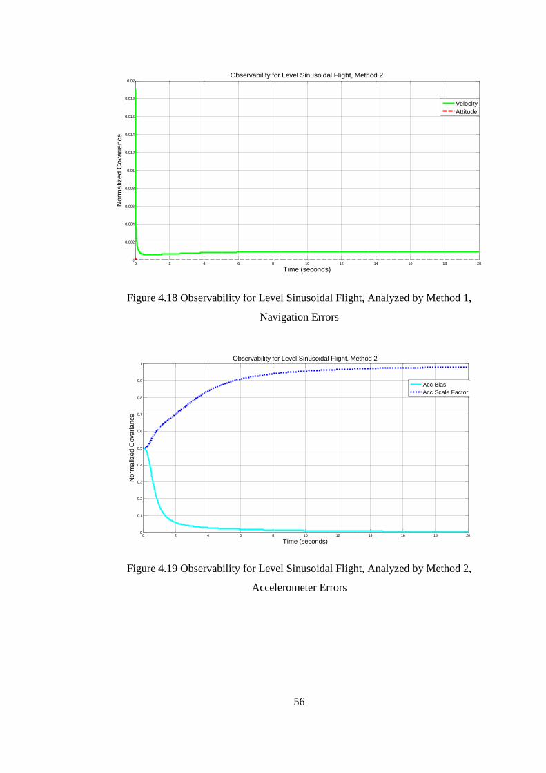
56


Navigation Errors



0 2 4 6 8 10 12 14 16 18 200

0.002

0.004

0.006

0.008

0.01

0.012

0.014

0.016

0.018

0.02

Time (seconds)

No

rma

lize

d C

ova

ria

nce


Velocity

Attitude

0 2 4 6 8 10 12 14 16 18 200

0.1

0.2

0.3

0.4

0.5

0.6

0.7

0.8

0.9

1

Time (seconds)

No

rma

lize

d C

ova

ria

nce


Acc Bias

Acc Scale Factor

57


Gyro Errors


Navigation Errors

0 2 4 6 8 10 12 14 16 18 200

0.1

0.2

0.3

0.4

0.5

0.6

0.7

0.8

0.9

1

Time (seconds)

No

rma

lize

d C

ova

ria

nce


Gyro Bias

Gyro Scale Factor

0 2 4 6 8 10 12 14 16 18 200

0.002

0.004

0.006

0.008

0.01

0.012

0.014

0.016

0.018

0.02

Time (seconds)

No

rma

lize

d C

ova

ria

nce


Velocity

Attitude

58

The optimum choice of maneuver for transfer alignment is the complete s-turn

maneuver. Especially gyro bias estimations become significantly better as a result

of the attitude change in the maneuver.



Figure 4.23 Observability for Sinusoidal Flight with Roll, Analyzed by Method 1, Gyro

Errors

0 2 4 6 8 10 12 14 16 18 20

0.4

0.5

0.6

0.7

0.8

0.9

1

1.1

Time (seconds)

Eig

en

Va

lue

OObservability for Level Sinusoidal Flight with Roll, Method 1

Acc Bias

Acc Scale Factor

0 2 4 6 8 10 12 14 16 18 200.2

0.3

0.4

0.5

0.6

0.7

0.8

0.9

1

1.1

1.2

Time (seconds)

Eig

en

Va

lue

Observability for Level Sinusoidal Flight with Roll, Method 1

Gyro Bias

Gyro Scale Factor

59


Navigation Errors



0 2 4 6 8 10 12 14 16 18 200

0.1

0.2

0.3

0.4

0.5

0.6

0.7

0.8

0.9

1

Time (seconds)

Eig

en

Va

lue


Velocity

Attitude

0 2 4 6 8 10 12 14 16 18 200

0.2

0.4

0.6

0.8

1

1.2

1.4

Time (seconds)

No

rma

lize

d C

ova

ria

nce


Acc Bias

Acc Scale Factor

60

Figure 4.26 Observability for Sinusoidal Flight with Roll, Analyzed by Method 2, Gyro

Errors


Navigation Errors

As a result of the observability analyses with both methods for different

maneuvers, a simple s-turn or similar maneuver with attitude change is showed to

be sufficient for rapid transfer alignment. The conventional transfer alignment is

0 2 4 6 8 10 12 14 16 18 200

0.1

0.2

0.3

0.4

0.5

0.6

0.7

0.8

0.9

1

Time (seconds)

No

rma

lize

d C

ova

ria

nce


Gyro Bias

Gyro Scale Factor

0 2 4 6 8 10 12 14 16 18 200

0.002

0.004

0.006

0.008

0.01

0.012

0.014

0.016

0.018

0.02

Time (seconds)

No

rma

lize

d C

ova

ria

nce


Velocity

Attitude

61

completed in approximately 1 to 5 minutes, whereas the rapid transfer alignment

algorithm in this thesis is completed in 10 seconds. It is shown that regardless of

the maneuver choice, gyro and accelerometers scale factor errors are not

observable. This is an inherent result of the MEMS inertial sensor noise

characteristics. As the noise of inertial sensors of the Slave INS are very high with

respect to the Helicopter’s INS, the relevant noise masks the low dynamic motion

and makes the scale factor errors stochastically unobservable. In this case,

importance of stochastic observability analyses is shown, where a simple

traditional observability analyses states that scale factor errors are observable with

these maneuvers [12].

The transfer alignment maneuver duration shall be such that when the maneuver is

finished, all states should have been converged to their steady state values. Thus,

transfer alignment time is determined by maneuver duration for necessary state

estimations.

62

CHAPTER 5

5 VIBRATION DEPENDENT INERTIAL SENSOR

ERRORS

Inertial sensors, especially MEMS based gyros and accelerometers are severely

affected from mechanical vibrations. The vibration sensitivity of MEMS sensors

arise from their working principle; a MEMS gyro is in fact a Coriolis vibratory

gyro. Whenever a mechanical vibration is applied to the MEMS sensor, the

vibration is mistaken as a measurement in angular rate due to its working

principle.

In the field use of MEMS sensors, especially in guided munitions, carrier based

vibrations arising from engine, blades or etc. are serious sources of errors. For

example, a MEMS based gyro may have a bias repeatability of 100 deg/hr, but a

bias shift of 600 deg/hr may occur in a vibratory environment. Note that these

error shifts are proportional to the vibration severity.

These vibration based errors are not permanent. When the vibration level

diminishes, the temporary bias shifts disappear. In the transfer alignment case,

there is a significant bias difference between the pre-launch and after launch

performance. This may result in a problem in the estimation of bias parameters.

The vibration spectrum present at the guided munitions’ IMU is driven by the host

platform’s environment that is captive carry environment. During this captive

63

carry process, the error levels are significantly higher relative to the free flight of

the munitions. Thus, the vibration based errors should be modeled in order to

calibrate the IMU in the transfer alignment phase.

Vibration based inertial sensor errors are bias and noise shifts, which are also

called g-squared shifts. In the following chapters, these error types will be

characterized by ground tests. Then, relevant modeling will be given.

In the literature, characterization of vibration environment is done to design a

mechanical vibration damper for MEMS sensors and IMUs. The dampers can

reduce the vibration levels that affect the performance of sensors, but they require

a significant amount of space to be installed in a guided munition and besides,

they may no filter out every single frequency input. In the helicopter based

vibration, main source of vibration is rotor blade rotation, which is between 4-10

Hz. The bandwidth of an IMU in missile applications is generally 50-80 Hz,

which means if a damper which filters out the rotor blade vibration is applied; the

real bandwidth of IMU will be less than ~4-10 Hz.

Thus, a solution without damper should be chosen for vibration problem. Most of

the inertial sensor errors can be factory calibrated such as bias offset, scale factor

error and misalignment. There is no study in the literature to compensate the

vibration dependent errors of inertial sensors. In this thesis, the vibration

dependent errors characterization and modeling is done by vibration table tests.

In order to calibrate vibration dependent errors in the flight, the vibration profile

of the carrier platform should be known. In order to determine this profile, flight

tests are carried out while measuring the high frequency motion of the launcher

pod. The change of vibration level and frequency distribution is shown to be

related with total velocity and loading configuration of the helicopter.

In the vibration tests of inertial sensors, it is shown that the main parameters that

change with vibration are bias and noise. As explained before, bias is pre

64

calibrated by the help of these tests. Noise is one of main parameters in the

Kalman filtering. If the noise variance is not correct, the filter performance will

certainly be non-optimum, even stability problems may occur. As the noise

variance is a function of vibration level, the process noise matrix can easily be

online adapted in the Kalman filter.

5.1 Effects of Vibration on Transfer Alignment Performance

In this chapter, effects of platform (Helicopter) vibrations, arising from main and

tail rotor, are analyzed. Vibration test is performed according to Mil Std. 810 F –

Method 514.5 [50]. The vibration test defined in this standard state the profile for

ground tests using a vibration table. For the host platform in this study, the

helicopter, the profile and relevant parameters are defined as follows;

Figure 5.1 Vibration Profile for Environmental Tests [50]

65

Table 5.1 Basic Parameters for Vibration Profile

Location Vibration Level Source Frequency Range (fx) Peak Acceleration at fx

General

W0= 0.0010 g2/Hz 3 to 10 0.70 /(10.70-fx)

W1= 0.010 g2/Hz 10 to 25 0.10 x fx

ft= 500 Hz 25 to 40 2.5

40 to 50 6.50-0.10xfx

50 to 500 1.5

Instrument Panel

W0= 0.0010 g2/Hz 3 to 10 0.70 /(10.70-fx)

W1= 0.010 g2/Hz 10 to 25 0.070 x fx

ft= 500 Hz 25 to 40 1.75

40 to 50 4.550-0.070xfx

50 to 500 1.05

External Stores

W0= 0.0020 g2/Hz 3 to 10 0.70 /(10.70-fx)

W1= 0.020 g2/Hz 10 to 25 0.150 x fx

ft= 500 Hz 25 to 40 3.75

40 to 50 9.750-0.150xfx

50 to 500 2.25

Table 5.2 Main and Tail Rotor Frequency Parameters

f1=1P f1=1T fundamental

f=n x1P f=mX1T blade passage

f=2xnx1P f=2xmX1T 1st Harmonic

f=3xnx1P f=3xmX1T 2nd Harmonic

Table 5.3 Drive Train Component Rotation Frequency Parameters

f=1S fundamental

F=2x1S 1st Harmonic

F=3x1S 2nd Harmonic

F=4x1S 3rd Harmonic

66

Table 5.4 Main and Tail Rotor Parameters

Helicopter

Main Rotor Tail Rotor

Rotation Speed (Hz)

Number of Blades

Rotation Speed (Hz)

Number of Blades

AH-1 5.4 2 27.7 2

AH-6J 7.8 5 47.5 2

AH64 4.82 4 23.4 4

UH-1 5.4 2 27.7 2

UH-60 4.3 4 19.8 4

The vibration table used in the tests works in an open loop manner; the vibration

profile is entered to the system at the beginning of the test and measured by its

own accelerometers in order to see whether the vibration profile is satisfied.

Sample measurement taken from vibration table can be seen in Figure 5.2

Figure 5.2 Vibration Profile measured in the test equipment

With the help of this test, the effects of Main Rotor (MR) and Tail Rotor (TR) can

be seen without any experimental data. Notice that main purpose of Mil-Std-810F

is to make a test to see effects of various environmental conditions for the worst

67

case that is the test profiles can be over safe. The real vibration profile may be

different than the profile shown in Figure 5.3. The Experimental vibration data is

given in the next part of this chapter. Besides, the vibration profile for different

flight condition should be determined. The standard ground test is the worst

condition, but the other conditions should also be examined in order to properly

calibrate the inertial sensors and adjust process noise parameters in the Kalman

Filter. But, for the initial analysis, the profile given in Mil-Std-810F is sufficient.

The tests are carried given vibration profile in Table 5.1-3 to see different levels

of the vibration. The IMU is attached to the vibration table with relevant

mechanical fixtures and it is exposed to vibration in each 3 three axes. The IMU

data collected from these tests are used in the Transfer Alignment Simulation. In

the algorithm results, effects of mechanical vibration are especially seen in the

IMU error parameters estimation. With the vibration effects inserted in the

simulation, it is clearly seen that bias estimation is severely affected; convergence

rates are reduced and steady state errors are increased.

Figure 5.3 X Accelerometer Bias Estimation with Random Vibration

0 10 20 30 40 50 60-0.02

0

0.02

0.04

0.06

0.08

0.1

0.12

0.14

Time

Bia

s E

stim

atio

n (

g)

X Accelerometer Bias Estimation

Ideal

Random Vibration applied

68

Figure 5.4 Y Accelerometer Bias Estimation with Random Vibration

Figure 5.5 Z Accelerometer Bias Estimation with Random Vibration

0 10 20 30 40 50 600

0.05

0.1

0.15

0.2

0.25

Time (s)

Bia

s (

g)

Y Accelerometer Bias Estimation

Ideal

Random Vibration Applied

0 10 20 30 40 50 600

0.05

0.1

0.15

0.2

0.25

0.3

0.35

Time (s)

Bia

s (

g)

Z Accelerometer Bias Estimation

Ideal


69

Figure 5.6 X Gyro Bias Estimation with Different Vibration Amplitudes

Figure 5.7 Y Gyro Bias Estimation with Random Vibration

0 10 20 30 40 50 600

0.05

0.1

0.15

0.2

0.25

0.3

0.35

Bia

s E

stim

atio

n (

de

g/s

)

Roll Gyro Bias Estimation

Time (s)

Ideal


0 10 20 30 40 50 60-0.1

0

0.1

0.2

0.3

0.4

0.5

0.6

Bia

s E

stim

atio

n (

de

g/s

)

Pitch Gyro Bias Estimation

Time (s)

Ideal


70

Figure 5.8 Z Gyro Bias Estimation with Random Vibration

As it seen from Figure 5.3 to Figure 5.8, the vibration arising from the host

platform, helicopter, has a significant effect on inertial sensor bias estimations.

The convergence rate and the steady state accuracy of both accelerometer and

gyro bias estimations are severely affected.

There are two main reasons behind these results;

The vibration applied to the guided munition by carrier platform results in

increased noise which was not taken into consideration in the Kalman

Filter

The biases of inertial sensors are shifted due to the mechanical vibration,

resulting in faulty estimation.

5.2 Characterization of Vibration Environment

The vibration effects in a helicopter are driven by the main rotor, the turbo shaft

engine, the gearboxes and the tail rotor. The main rotor vibrations arise from an

0 10 20 30 40 50 600

0.1

0.2

0.3

0.4

0.5

0.6

0.7

0.8

0.9

Time (s)

Bia

s E

stim

atio

n (

de

g/s

)

Yaw Gyro Bias Estimation

Ideal


71

asymmetric distribution of the unsteady aerodynamic forces on the blades and

depend on the number of blades and the rotation rate. The speed of the main rotor

is generally kept constant, but the amplitude of the vibrations changes with

different flight phases, such as hover in/out of ground effect, different cruise

speeds etc. In most of the helicopters, vibration suppression system is designed for

a specific cruise speed, but the transfer alignment may have to be accomplished in

different speeds. Also, the vibration amplitude in the missile pylon can change

with the loading configuration, i.e. the number of munitions in the launching pod.

In order to characterize the vibration environment, accelerometer measurements

are taken from the launcher for different flight phases with different loading

configurations.

Figure 5.9 Vibration Profile for Hover in Ground Effect

101

102

103

10-5

Frequency (Hz)

Acce

lera

tio

n S

pe

ctr

al D

en

sity (

g 2 / H

z)

Vibration Profile for Hover in Ground Effect

0 500 1000 1500 2000 2500 3000 3500 4000

10-5

Frequency (Hz)

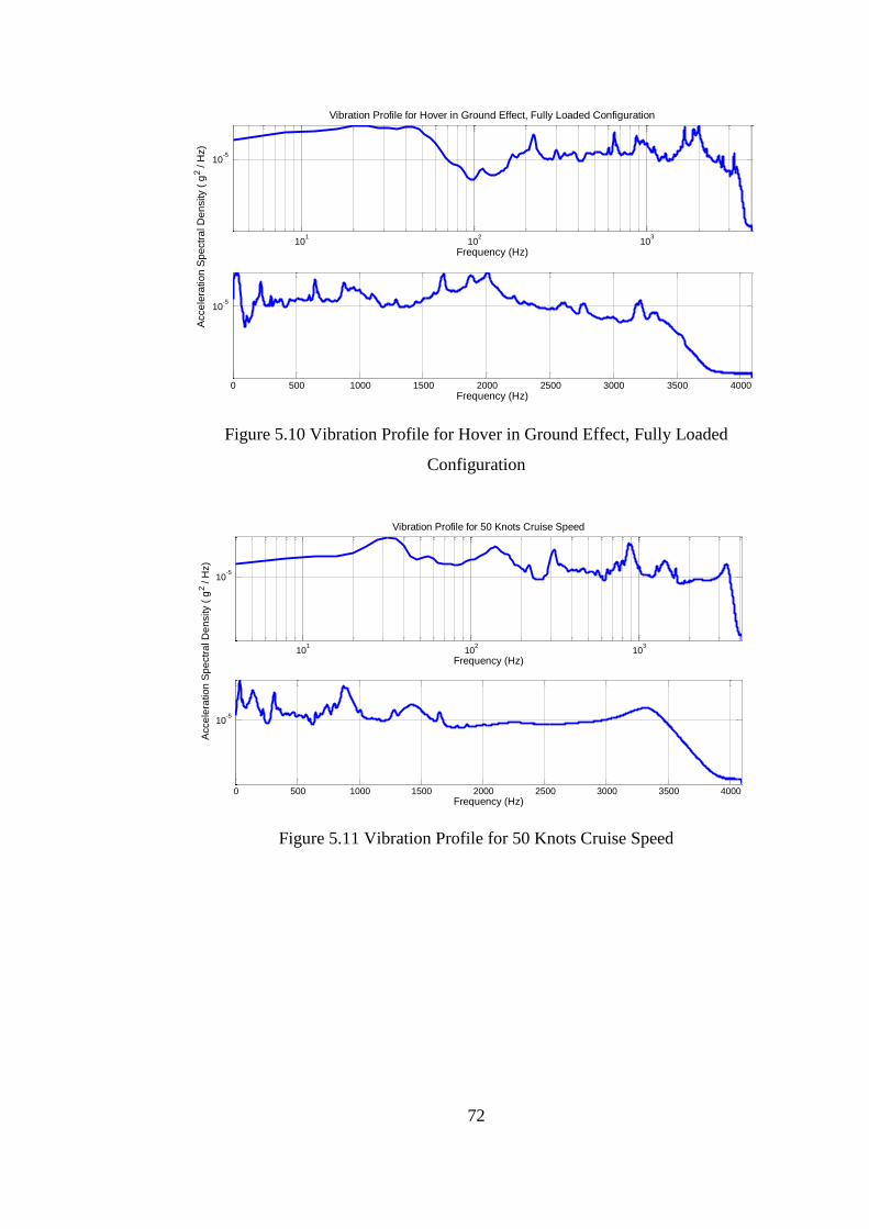
72

Figure 5.10 Vibration Profile for Hover in Ground Effect, Fully Loaded

Configuration

Figure 5.11 Vibration Profile for 50 Knots Cruise Speed

101

102

103

10-5

Frequency (Hz)

Acce

lera

tio

n S

pe

ctr

al D

en

sity (

g 2 / H

z)

Vibration Profile for Hover in Ground Effect, Fully Loaded Configuration

0 500 1000 1500 2000 2500 3000 3500 4000

10-5

Frequency (Hz)

101

102

103

10-5

Frequency (Hz)

Acce

lera

tio

n S

pe

ctr

al D

en

sity (

g 2 / H

z)

Vibration Profile for 50 Knots Cruise Speed

0 500 1000 1500 2000 2500 3000 3500 4000

10-5

Frequency (Hz)

73


Configuration


101

102

103

10-5

Frequency (Hz)

Acce

lera

tio

n S

pe

ctr

al D

en

sity (

g 2 / H

z)

Vibration Profile for 50 Knots Cruise Speed, Fully Loaded Configuration

0 500 1000 1500 2000 2500 3000 3500 4000

10-5

Frequency (Hz)

101

102

103

10-5

Frequency (Hz)

Acce

lera

tio

n S

pe

ctr

al D

en

sity (

g 2 / H

z)


0 500 1000 1500 2000 2500 3000 3500 4000

10-5

Frequency (Hz)

74


Configuration


101

102

103

10-5

Frequency (Hz)

Acce

lera

tio

n S

pe

ctr

al D

en

sity (

g 2 / H

z)


0 500 1000 1500 2000 2500 3000 3500 4000

10-5

Frequency (Hz)

101

102

103

10-5

Frequency (Hz)

Acce

lera

tio

n S

pe

ctr

al D

en

sity (

g 2 / H

z)


0 500 1000 1500 2000 2500 3000 3500 4000

10-5

Frequency (Hz)

75


Configuration

From Figure 5.9 to Figure 5.16, it is shown that vibration profile of the Slave INS

is dependent on two parameters, platform velocity and munition loading

configuration. A simple look-up table gives the relation between these two

parameters and slave INS vibration level.

5.3 Characterization of Vibration Dependent Errors

MEMS inertial sensors are the most severely affected sensor technology from

platform mechanical vibrations. This is a fact of its sensing methodology, MEMS

sensors uses a vibratory method to sense the angular rates or accelerations. For

example, most of the MEMS gyros are also known as Coriolis vibratory gyro.

Almost all of the MEMS sensors have resonant frequency of approximately

14Khz. In the military standard Mil-Std-810, the platform vibration is defined as a

random vibration profile with a frequency range between 20Hz and 2.6 Khz. In

order to see the effect of these vibration profile, several tests are done with

different vibration spectrum, 2.1g RMS, 4.2g RMS and 7.6g RMS. Sample test

results for gyros are given below, where bias and noise shift can easily be seen.

101

102

103

10-5

Frequency (Hz)

Acce

lera

tio

n S

pe

ctr

al D

en

sity (

g 2 / H

z)


0 500 1000 1500 2000 2500 3000 3500 4000

10-5

Frequency (Hz)

76

Figure 5.17 Pitch Gyro Output for Vibration Profile, 4.2 g RMS

Figure 5.18 Pitch Gyro Output for Vibration Profile, 7.6 g RMS

0 0.2 0.4 0.6 0.8 1 1.2 1.4 1.6 1.8 2

x 105

-30

-25

-20

-15

-10

-5

0

5

10

Time (ms)

Se

nso

r O

utp

ut,d

eg

/se

c

Vibration Test for Pitch Gyro, 4.2 g RMS

Data

Moving Average

0 0.2 0.4 0.6 0.8 1 1.2 1.4 1.6 1.8 2

x 105

-40

-30

-20

-10

0

10

20

Time (ms)

Se

nso

r O

utp

ut,d

eg

/se

c

Vibration Profile for Pitch Gyro, 7.6g RMS

Data

Moving Average

77

Figure 5.19 Roll Gyro Output for Vibration Profile, 4.2 g RMS

Figure 5.20 Roll Gyro Output for Vibration Profile, 7.6 g RMS

0 0.2 0.4 0.6 0.8 1 1.2 1.4 1.6 1.8 2

x 105

-16

-14

-12

-10

-8

-6

-4

-2

0

Time (ms)

Se

nso

r O

utp

ut,d

eg

/se

c

Vibration Test for Roll Gyro, 4.2 g RMS

Data

Moving Average

0 0.2 0.4 0.6 0.8 1 1.2 1.4 1.6 1.8 2

x 105

-20

-18

-16

-14

-12

-10

-8

-6

-4

-2

0

Time (ms)

Se

nso

r O

utp

ut,d

eg

/se

c

Vibration Test for Roll Gyro, 7.6 g RMS

Data

Moving Average

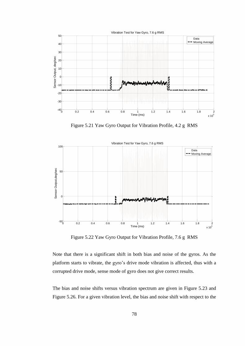
78

Figure 5.21 Yaw Gyro Output for Vibration Profile, 4.2 g RMS

Figure 5.22 Yaw Gyro Output for Vibration Profile, 7.6 g RMS

Note that there is a significant shift in both bias and noise of the gyros. As the

platform starts to vibrate, the gyro’s drive mode vibration is affected, thus with a

corrupted drive mode, sense mode of gyro does not give correct results.

The bias and noise shifts versus vibration spectrum are given in Figure 5.23 and

Figure 5.26. For a given vibration level, the bias and noise shift with respect to the

0 0.2 0.4 0.6 0.8 1 1.2 1.4 1.6 1.8 2

x 105

-40

-30

-20

-10

0

10

20

30

40

50

Time (ms)

Se

nso

r O

utp

ut, d

eg

/se

c

Vibration Test for Yaw Gyro, 7.6 g RMS

Data

Moving Average

0 0.2 0.4 0.6 0.8 1 1.2 1.4 1.6 1.8 2

x 105

-50

0

50

100

Time (ms)

Se

nso

r O

utp

ut,d

eg

/se

c

Vibration Test for Yaw Gyro, 7.6 g RMS

Data

Moving Average

79

nominal condition can easily be found, where vibration level can be obtained for a

given velocity and loading configuration.

Figure 5.23 Gyro Noise Shift with respect to vibration level

80

Figure 5.24 Accelerometer Noise Shift with respect to vibration level

Figure 5.25 Gyro Bias Shift with respect to vibration level

81

Figure 5.26 Accelerometer Bias Shift with respect to vibration level

With the help of these tests, the vibration induced bias shift can now be in flight

calibrated for a given flight velocity, thus the bias estimation errors in the Transfer

Alignment can be significantly reduced. Another important outcome of these tests

is the noise variance modeling. The process noise in the Kalman Filter of Transfer

Alignment can now be adaptively changed for a given flight condition, thus

keeping the estimation in an optimum manner.

82

CHAPTER 6

6 FLEXIBLE LEVER ARM

IN TRANSFER ALIGNMENT

6.1 Characterization of Flexible Lever Arm

In rapid transfer alignment, attitude matching between master and slave INSs is

done with rigid body lever arm compensation. This compensation of relative

orientation can be easily done as the rigid body lever arm is measured and entered

to the database of transfer alignment algorithm in the design phase. There will be

static errors arising from manufacturing and mounting errors in the platform,

which are small enough to be neglected in transfer alignment

But, for most of the platforms in the transfer alignment, this relative orientation is

not rigid, instead it is highly flexible. The flexure in the host platform is generally

is a function of aerodynamics and structural forcers, thus the complete dynamics

of this flexible lever arm becomes highly complicated. In the literature, most of

the rapid transfer alignment studies deals with this effect by increasing the

measurement noise covariance, thus reducing the steady state accuracy in the

transfer alignment. Another method is to model this flexible lever arm effect as a

first or second order Markov process and augmenting it as filter states in the

transfer alignment.

83

In this thesis, the flexible lever arm will be modeled in two different manners,

with Markov process state augmentation and a artificial neural network approach.

Details are given in the following parts of the thesis.

The first step in the modeling of flexible lever arm modeling is the

characterization stage. Experimental data is collected in order to characterize the

dynamics of the level arm. In the data acquisition, high accuracy navigation grade

INS is added to the munition pod. Basically, the difference between the two INSs

gives the lever arm orientation;

n Platform n

b Munition Munition b PlatformC C C (6.1)

1( )Platform n n

Munition b Munition b PlatformC C C (6.2)

As both INSs are navigation grade, their attitude error can be easily neglected.

One of the trajectories used in data acquisition is described in Table 6.1 as an

example.

Table 6.1 Segments of the Trajectory

Segment Number Maneuver Type

1 Ground Run

2 Take off

3 Hover

4 Climb

5 Straight Climb

6 Cruise

7 Heading Change

8 Cruise

9 Climbing Turn

10 Straight Descend

11 Cruise

12 Level Flight Turn

13 Racetrack

14 Cruise

15 Hover

16 Landing

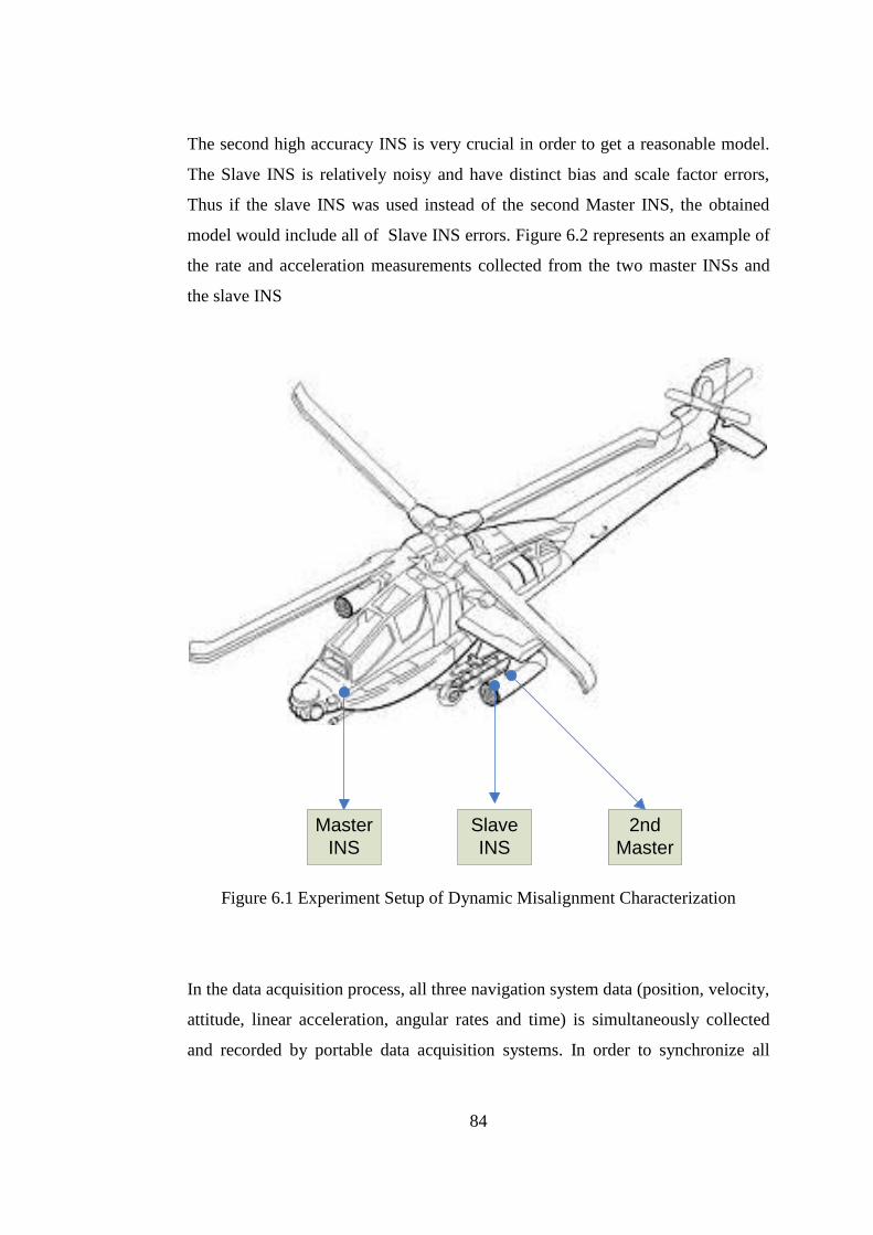
84

The second high accuracy INS is very crucial in order to get a reasonable model.

The Slave INS is relatively noisy and have distinct bias and scale factor errors,

Thus if the slave INS was used instead of the second Master INS, the obtained

model would include all of Slave INS errors. Figure 6.2 represents an example of

the rate and acceleration measurements collected from the two master INSs and

the slave INS

Figure 6.1 Experiment Setup of Dynamic Misalignment Characterization

In the data acquisition process, all three navigation system data (position, velocity,

attitude, linear acceleration, angular rates and time) is simultaneously collected

and recorded by portable data acquisition systems. In order to synchronize all

Master

INS

Slave

INS

2nd

Master

85

three navigation systems, time data of each system is also recorded. Data

acquisition is done several times for different maneuver agilities and loading

configurations.

Once the data acquisition is completed, the dynamic misalignment is analyzed

separately for each trajectory segment, maneuvers and loading configurations.

As it is stated in the previous chapter, the captive carry vibration characteristics of

a helicopter launched guided munition is dependent on the platform velocity and

the loading configuration. Same situation occurs for dynamic misalignment. In

order to characterize the dynamic misalignment and model it accurately,

experimental data is collected for different cruise speeds and loading

configurations.

Figure 6.2 to Figure 6.20 illustrates the flexible orientation dynamics for different

flight phases and velocities.

Figure 6.2 Dynamic Roll Misalignment for Hover

0 5 10 15 20 25 30 35 40 45 50-0.4

-0.3

-0.2

-0.1

0

0.1

0.2

0.3

0.4 Roll Attitude Misalignment between Master and Slave

Time, seconds

Ro

ll D

iffe

ren

ce

,de

g

86

Figure 6.3 Dynamic Roll Misalignment for Hover, Fully Loaded Configuration

Figure 6.4 Dynamic Pitch Misalignment for Hover

0 5 10 15 20 25 30 35 40 45 50-0.5

-0.4

-0.3

-0.2

-0.1

0

0.1

0.2

0.3

0.4


Time, seconds

Ro

ll D

iffe

ren

ce

,de

g

0 5 10 15 20 25 30 35 40 45 50-0.4

-0.3

-0.2

-0.1

0

0.1

0.2

0.3

0.4

0.5 Pitch Attitude Misalignment between Master and Slave

Time, seconds

Pitch

Diffe

ren

ce

,de

g

87

Figure 6.5 Dynamic Pitch Misalignment for Hover, Fully Loaded Configuration

Figure 6.6 Dynamic Yaw Misalignment for Hover

0 5 10 15 20 25 30 35 40 45 50-0.4

-0.3

-0.2

-0.1

0

0.1

0.2

0.3

0.4


Time, seconds

Pitch

Diffe

ren

ce

,de

g

88

Figure 6.7 Dynamic Roll Misalignment for 50 Knots Cruise Speed


Configuration

0 5 10 15 20 25 30 35 40 45 50-0.5

-0.4

-0.3

-0.2

-0.1

0

0.1

0.2

0.3

0.4


Time, seconds

Ro

ll D

iffe

ren

ce

,de

g

0 5 10 15 20 25 30 35 40 45 50-0.8

-0.6

-0.4

-0.2

0

0.2

0.4


Time, seconds

Ro

ll D

iffe

ren

ce

,de

g

89

Figure 6.9 Dynamic Pitch Misalignment for 50 Knots Cruise Speed


Loaded Configuration

0 5 10 15 20 25 30 35 40 45 50-0.8

-0.6

-0.4

-0.2

0

0.2

0.4


Time, seconds

Pitch

Diffe

ren

ce

,de

g

0 5 10 15 20 25 30 35 40 45 50-0.8

-0.6

-0.4

-0.2

0

0.2

0.4


Time, seconds

Pitch

Diffe

ren

ce

,de

g

90

Figure 6.11 Dynamic Yaw Misalignment for 50 Knots Cruise Speed


0 5 10 15 20 25 30 35 40 45 50-0.5

-0.4

-0.3

-0.2

-0.1

0

0.1

0.2

0.3

0.4


Time, seconds

Ro

ll D

iffe

ren

ce

,de

g

91


Configuration


0 5 10 15 20 25 30 35 40 45 50-0.8

-0.6

-0.4

-0.2

0

0.2

0.4


Time, seconds

Ro

ll D

iffe

ren

ce

,de

g

0 5 10 15 20 25 30 35 40 45 50-0.8

-0.6

-0.4

-0.2

0

0.2

0.4


Time, seconds

Pitch

Diffe

ren

ce

,de

g

92



Figure 6.16 Dynamic Yaw Misalignment for 70 Knots Cruise Speed

0 5 10 15 20 25 30 35 40 45 50-0.5

-0.4

-0.3

-0.2

-0.1

0

0.1

0.2

0.3

0.4


Time, seconds

Pitch

Diffe

ren

ce

,de

g

93


Figure 6.18 Dynamic Roll Misalignment for 100 Knots Cruise Speed, Fully


0 5 10 15 20 25 30 35 40 45 50-0.8

-0.6

-0.4

-0.2

0

0.2

0.4

0.6

Roll Attitude Misalignment between Master and Slave

Time, seconds

Ro

ll D

iffe

ren

ce

,de

g

0 5 10 15 20 25 30 35 40 45 50-0.8

-0.6

-0.4

-0.2

0

0.2

0.4


Time, seconds

Ro

ll D

iffe

ren

ce

,de

g

94




The experimental data shows that roll and pitch attitude are severely affected from

the low frequency vibrations, whereas the flexibility in yaw channel is almost

negligible. As in the high frequency vibration profiles, the frequency distribution

is almost constant for different flight phases, but the amplitude changes.

0 5 10 15 20 25 30 35 40 45 50-0.8

-0.6

-0.4

-0.2

0

0.2

0.4

0.6

Pitch Attitude Misalignment between Master and Slave

Time, seconds

Pitch

Diffe

ren

ce

,de

g

0 5 10 15 20 25 30 35 40 45 50-0.8

-0.6

-0.4

-0.2

0

0.2

0.4

0.6


Time, seconds

Pitch

Diffe

ren

ce

,de

g

95

Throughout the experiments, the dynamic misalignment between the helicopter’s

(master) and munition’s (slave) INSs have the same frequency profile for different

trajectory segments. Also, there is no significant transient motion between the

transition of two trajectory segments. It is shown that the dynamic misalignment

have a constant frequency distribution for a given total velocity and loading

configuration, similar to high frequency vibration shown in Chapter 5. This is an

important outcome especially for modeling approaches. In the aircraft based

transfer alignment studies, it is shown that transient effects are serious problem

for modeling of dynamic misalignment. In the aircrafts, especially on the

coordinated turn maneuvers, the force loading on the wings increase, thus both

static and dynamic wing deflection changes. In the helicopter based transfer

alignment, the force loading on launcher pod is almost constant as the forcing

sources, main and tail rotor vibration, are constant. This is an important advantage

compared to aircraft transfer alignment, where modeling of dynamic

misalignment is very complicated due to the transient effects.

6.2 Error Modeling Approaches

Dynamic misalignment compensation is important to improve the accuracy and

speed of the transfer alignment process. The flight data showed that the

misalignment between master and slave INSs have a distinct characteristic which

directly depends on the host platform’s mission profile.

In the literature, the modeling of dynamic misalignment is generally handled as

simple white noise [3, 4, 5, 7, 8, 10, and 11]. By this approach, the computational

load of the Kalman filter is kept in minimum level, but the accuracy is severely

reduced [22, 23, 24, 26]. As showed in part 6.1, the misalignment is certainly not

white noise; it is correlated by different frequencies. In the aircraft based transfer

alignment studies, there is no detailed characterization of dynamic misalignment

for transfer alignment. Reference 26 is the unique study that deals with this

flexibility effect by an analytical modeling approach. The wing deflection is

96

modeled by finite element method for different flight conditions and this model is

applied in transfer alignment to compensate the dynamic and static misalignment

based errors.

Modeling of dynamic misalignment as only white noise is only done for filter

stability [7, 8, 10, and 24]. This approach results in reduced steady state error and

convergence rate.

As stated in Chapter 1, there is no detailed study for helicopter based transfer

alignment, especially for dynamic misalignment. Different from aircraft based

transfer alignment; the misalignment has a steady frequency characteristic,

transient effects are negligible as shown in Chapter 6.1

Dynamic misalignment compensation is handled by two different methods;

State augmentation

Artificial Neural Network

As stated previously, some of the transfer alignment studies [3,4,7,8 and 17]

models the flexible orientation between the master and slave INS as Markov

processes. In these studies, the Markov processes are used only for analysis, not

for accurate compensation. The dynamic misalignment is not characterized by

experiments or analytical methods. A simple first or second order Markov process

is used to model the possible effects on Transfer Alignment. In this thesis,

experimental data is used to find an accurate model.

The second method is to use artificial neural network to compensate dynamic

misalignment outside of the Kalman Filter. Artificial neural network is trained

offline by experimental data. ANNs are generally trained online by back

propagation technique, which may not be practical in Transfer Alignment. The

required training data is the dynamic misalignment data between the helicopter

and launcher INSs, which is recorded by the experimental setup described in

97

Chapter 6.1. In order to do the neural network training online, slave INS data

instead of 2nd

master INS should be used. In this case, all errors present in guided

munition’s INS will be integrated into ANN, thus the final performance and

accuracy of transfer alignment will be severely affected. By using offline training

method, these errors are avoided.

Note that the dynamic misalignment values are less than 1-2 degrees in all flight

cases; roll and pitch misalignment can be taken as uncoupled. Thus, instead of

having one complex model, there will be two simple model for pitch and roll

misalignment, both in state augmentation and neural network.

6.2.1 State Augmentation

In the literature [3-8, 17, 23 and 34], state augmentation for dynamic

misalignment is generally used for offline analysis. For online estimation and

compensation of dynamic misalignments, experimental data shown in Chapter 6.1

is used.

As it is easily seen from the experimental data, the flexibility in roll and pitch

channels are near harmonic, thus at least second order model is required. In the

yaw channel, the dynamics is distinctly lower than the others, so it can be

neglected. In order to obtain an accurate model;

Order of the Markov Process is to be determined.

Parameters of Markov Process should be tuned with experimental data.

Order determination of Markov processes for a given data is the important part in

state estimation. The order of the model should be high enough to model the

system accurately, but should not be very high in order to augment it to the

Kalman Filter without high computational load.

In the literature, first or second order Markov processes are used. But, these

studies are only done for aircraft launched systems. In the helicopter based

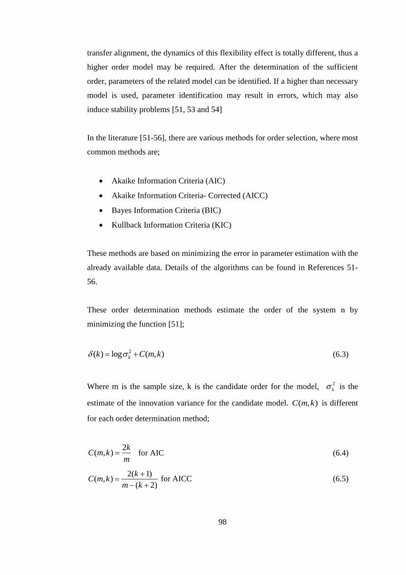
98

transfer alignment, the dynamics of this flexibility effect is totally different, thus a

higher order model may be required. After the determination of the sufficient

order, parameters of the related model can be identified. If a higher than necessary

model is used, parameter identification may result in errors, which may also

induce stability problems [51, 53 and 54]

In the literature [51-56], there are various methods for order selection, where most

common methods are;

Akaike Information Criteria (AIC)

Akaike Information Criteria- Corrected (AICC)

Bayes Information Criteria (BIC)

Kullback Information Criteria (KIC)

These methods are based on minimizing the error in parameter estimation with the

already available data. Details of the algorithms can be found in References 51-

56.

These order determination methods estimate the order of the system n by

minimizing the function [51];

2( ) log ( , )kk C m k (6.3)

Where m is the sample size, k is the candidate order for the model, 2

k is the

estimate of the innovation variance for the candidate model. ( , )C m k is different

for each order determination method;

2( , )

kC m k

m for AIC (6.4)

2( 1)( , )

( 2)

kC m k

m k

for AICC (6.5)

99

log( )( , )

m kC m k

m for BIC (6.6)

2log log( )( , ) ,

m kC m k KIC

m (6.7)

The penalty factor C(m,k) is the main difference between the order determination

methods. For example, AIC and AICC are derived or unbiased estimation, while

KIC minimizes the final prediction error [56].

The summary of the order determination results are as follows;

Table 6.2 Order Determination for State Augmentation

Method Model Order

1 2 3 4 5

AIC 2.8 56.1 23.1 4.1 2.5

AICC 1.8 49.1 10.7 4.8 3.9

BIC 1.6 35.9 12.5 5.7 3.2

KIC 3.7 65.7 8.6 5.4 1.2

The appropriate order is determined by the maximum value of e equation 6.3. The

relative comparison of orders for the result of equation 6.3 indicates the difference

of probable error between different model orders. The criterion is the maximum

value of equation 6.3 between possible orders of model.

As stated above, there are different methods for C(m,k) in equation 6.3, in which

all dedicates minimization of different error criterions. Thus, possible four

different penalty functions are used (AIC, AICC, BIC and KIC) and the results are

compared. Table 6.2 summarizes the results of equation 6.3 by these methods for

model orders up to 5. It is seen that all four methods gives consistent results. As it

is seen from Table 6.2, second order model is the optimum choice for state

augmentation, indicated by all four methods. The resulting equation is given

below;

100

1 1 2 2t t t ty a y a y (6.8)

Where a1 and a2 are model parameters and t is the estimated innovation.

Next step in state augmentation is the parameter identification in the Markov

Process. There are three common methods that are used to determine the model

parameters [54-56];

Least Squares

Yule Walker

Burg

Generally, a sufficiently large data cluster yields approximately same parameter

estimation with these three methods [53, 55]. But it is shown in reference 54 that a

noisy harmonic data may result to incorrect parameter estimation or the final

system may be unstable.

In the following part, these three methods ( least squares, Yule walker and Burg)

are summarized;

Least squares methods results in a linear system of equation

11 1 1 01

1 0

p

p pp p p

c c a c

c c a c

(6.9)

Where,

1

1 N

ij t i t j

t p

c y yN p

(6.10)

101

Yule Walker method differs from Least squares by including first and last point

in equation (6.10) in order to obtain an unbiased estimation;

0 1 1 1

1 0

p

p p p

R R a R

R R a R

(6.11)

Where;

1

1 N

t t

t

R y yN

(6.12)

Usually, least squares or Yule-Walker method is used to determine the model

parameters, but as stated in [53,54,56], for periodic data, these methods lead to

incorrect estimation of parameters. For harmonic signals Burg’s method should be

used.

Burg’s method [56] does not directly estimate model parameters, instead of this,

the method estimates the reflection coefficients, the last model parameter estimate

for each model order p. Details of the Burg method can be found in Reference 56.

Least squares method is not used as it can result in an unstable Markov process. In

order to choose between Burg and Yule Walker methods, a sample analysis is

done. Comparison of Burg and Yule Walker Method’s are given in the following

figures. Same experimental data is used to find the parameters of the second order

Markov process, where their performance is as follows;

102

Figure 6.21 Performance Comparison of Yule Walker and Burg Method

The mean errors are nearly same for Yule Walker and Burg’s method, 0.003 and

0.00027 degrees, but the standard deviations of the errors are quite different. The

Yule walker method results in 0.17 degrees errors for standard deviation, while

Burg method results in 0.086 degrees. The accuracy of Burg method is nearly

twice of the Yule walker method.

As expected, Burg method results in a better Markov Model performance as the

experimental data is quite periodic.

In chapter 6.1, it was shown that the dynamic misalignment is dependent on two

different factors; the total speed of the helicopter and the loading configuration of

the launcher. The parameters a1 and a2 for the second order model given by

equation 6.8 are identified for these different flight conditions, given in the

following figures

103

Figure 6.22 a1 Parameter vs. Flight Velocity and Loading Configuration

Figure 6.23 a2 Parameter vs. Flight Velocity and Loading Configuration

As it can be seen from Figure 6.22 and Figure 6.23, a1 parameter heavily depends

on flight conditions, where a2 parameter is almost constant

0 10 20 30 40 50 60 70 80 90 1001.5

2

2.5

3

3.5

4

4.5

5

5.5 A1 Parameter vs Flight Velocity and Loading

Flight Velocity, Knots

A

1 p

ara

me

ter

Minimum Loading Configuration

Maximum Loading Configuration

0 10 20 30 40 50 60 70 80 90 100908.4

908.6

908.8

909

909.2

909.4

909.6

909.8 A2 Parameter vs Flight Velocity and Loading

Flight Velocity, Knots

A

2 p

ara

me

ter

Minimum Loading Configuration

Maximum Loading Configuration

104

6.2.2 Artificial Neural Network

Artificial neural networks are (ANN) used in many applications in the literature.

In this study, ANN is used to model and compensate dynamic misalignment. With

the pre-recorded data, ANN will be trained to obtain an estimation of flexible

misalignment. Thus, the lever arm compensation will be adaptively improved.

There are two important steps in the design of an artificial neural network; the

input / outputs of ANN and training method. As given in Chapter 6.1, there are

various dynamic misalignment data collected by experiments for different

trajectories and maneuvers. By installing the second master INS, the dynamic

misalignment data is collected for different flight conditions.

As stated in the previous parts, the flexible lever arm between the master and

slave IMUs in the helicopters has a velocity dependent behavior.

Figure 6.24 Artificial Neural Network Input Output Structure

Mainly, the amplitude and frequency distribution of this flexibility has a periodic

sinusoidal type character. The frequency characteristic of this motion does not

change with respect to the flight profile but the amplitude is proportional to the

helicopter’s velocity. Note that another input to the artificial neural network is the

loading configuration of the helicopter. As shown in the previous parts, loading of

the pylons directly affects the vibration amplitude of the slave IMUs. Most of the

Artificial Neural Network

Platform Velocity

Misalignment

Estimation

Master-Slave

Misalignment (from

Slave IMU)

Loading

Configuration

105

guided munition launcher pods can host up to 24 low caliber munitions. The

weight of the launcher pod is proportional to the number of hosted munitions and

the vibration amplitude level is increased with the weight of the pod. Thus, an

ANN will be used to compensate the flexible lever arm effect. Prerecorded flight

data is used to train the ANN.

Thus, there are three inputs and one output for dynamic misalignment estimation.

The inputs are Helicopter (platform) velocity, slave IMU measurement and

loading configurations. Helicopter velocity and loading configuration is directly

transferred from Helicopter to the guided munition. The important part in the

input structure is the use of Slave IMU measurements. The ANN may be

configured such that there is no need for slave IMU measurements, but there may

be synchronization problem for the estimation. The offline trained neural network

would have no information about the instantaneous motion of the launcher pod,

thus this phase difference would result in reduced accuracy. Thus, in order to keep

this phase difference in minimum Slave IMU inputs are included in the ANN

input structure.

For estimation purposes, usually Multilayer feed forward structure [44-48] is used

in ANN. The number of nodes and layers in ANN depends on the detail level and

complexity of estimated system. There is no specific method to determine these

parameters. ANNs used in navigation systems generally implements a 2 layer

structure. In order to determine the layer and node number, namely the topology

of ANN, different combinations are compared, shown in Table 6.4. In Table 6.4,

the results of a sample analysis of dynamic misalignment estimation are given;

similar to the analysis of parameter identification method case given in Chapter

6.2.1. In Table 6.4, the estimation errors for different layer structures of ANN are

given. The purpose of this analysis is to determine the sufficient artificial neural

network layer and node numbers. A less than sufficient layer and node number

may not be able to estimate the dynamic misalignment with the required accuracy,

whereas an unnecessary number of layers may results in an untrainable system;

106

that the training data may not be enough to train all the weights in the artificial

neural network.

Table 6.4 Structure combinations for ANN

Number of Layers Structure Error(1 , deg)

1 3x3x1 0.0976

1 3x2x1 0.113

2 3x3x3x1 0.0714

2 3x3x2x1 0.0742

2 3x2x3x1 0.0736

2 3x2x2x1 0.0753

As it is shown in Table 2, 2 layer combinations perform better than 1 layer

combinations. There is a difference of approximately %20 in the estimation error

between one and two layer artificial neural networks. The second part to examine

in the ANN design is the structure determination. As it is seen from Table 6.4, the

difference between the 2 layer structures is less than %5. Thus, in order to

optimize the artificial neural network, 3x2x2x1 structure is used, having optimum

accuracy with the minimum node number. The resulting configuration is shown

below;

Figure 6.25 Artificial Neural Structure for Dynamic Misalignment Estimation

For learning algorithm, different methods can be used such as;

Gradient Descent

Platform

Velocity

Slave

IMU

Loading

Dynamic

Misalignment

107

Gradient Descent with Adaptive Step Size

Simulated Annealing

Conjugate Gradient

Levenberg- Marquardt

These methods’ performance mainly differs in convergence rate [44, 47]. For

dynamic misalignment estimation, the training will be done offline, so

convergence rate is not a criterion for selection. Levenberg – Marquardt is chosed

as back propagation learning algorithm.

Briefly, 2 layer feedforward ANN will be utilized for this purpose. Details of the

ANN algorithm is given in Appendix C. Pre recorded flight data will be used for

training. Levenberg –Marquadt is used for learning algorithm.

6.2.3 Comparison of Methods

The difference between the neural network and state augmentation approaches are

shown in the below example cases;

Hover

50 Knots Cruise

70 Knots Cruise

100 Knots Cruise

Note that, these are the experiment cases defined in Table 6.1 for dynamic

misalignment data acquisition.

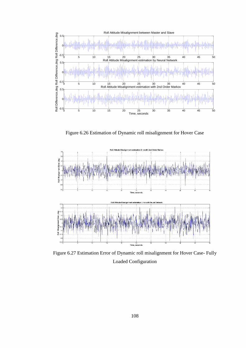
108

Figure 6.26 Estimation of Dynamic roll misalignment for Hover Case

Figure 6.27 Estimation Error of Dynamic roll misalignment for Hover Case- Fully


0 5 10 15 20 25 30 35 40 45 50-0.5

0


Ro

ll D

iffe

ren

ce

,de

g

0 5 10 15 20 25 30 35 40 45 50-0.5

0

0.5 Roll Attitude Misalignment estimation by Neural Network

Ro

ll D

iffe

ren

ce

,de

g

0 5 10 15 20 25 30 35 40 45 50-0.5

0

0.5 Roll Attitude Misalignment estimation with 2nd Order Markov

Time, seconds

Ro

ll D

iffe

ren

ce

,de

g

109

Figure 6.28 Estimation of Dynamic roll misalignment for Hover Case, Fully


Figure 6.29 Estimation Error of Dynamic roll misalignment for Hover Case, Fully


0 5 10 15 20 25 30 35 40 45 50-0.5

0


Ro

ll D

iffe

ren

ce

,de

g

0 5 10 15 20 25 30 35 40 45 50-0.5

0

0.5

1 Roll Attitude Misalignment estimation by Neural Network

Ro

ll D

iffe

ren

ce

,de

g

0 5 10 15 20 25 30 35 40 45 50-0.5

0

0.5 Roll Attitude Misalignment estimation with 2nd Order Markov

Time, seconds

Ro

ll D

iffe

ren

ce

,de

g

0 5 10 15 20 25 30 35 40 45 50-0.4

-0.2

0

0.2

0.4 Roll Attitude Misalignment estimation Errorwith 2nd Order Markov

Time, seconds

Ro

ll M

isa

lign

me

nt E

rro

r ,d

eg

0 5 10 15 20 25 30 35 40 45 50-0.4

-0.2

0

0.2

0.4 Roll Attitude Misalignment estimation Error with Neural Network

Time, seconds

Ro

ll M

isa

lign

me

nt E

rro

r ,d

eg

110

Figure 6.30 Estimation of Dynamic pitch misalignment for Hover Case

Figure 6.31 Estimation Error of Dynamic pitch misalignment for Hover Case

0 5 10 15 20 25 30 35 40 45 50-0.5

0


Pitch

Diffe

ren

ce

,de

g

0 5 10 15 20 25 30 35 40 45 50-0.5

0

0.5 Pitch Attitude Misalignment estimation by Neural Network

Pitch

Diffe

ren

ce

,de

g

0 5 10 15 20 25 30 35 40 45 50-0.5

0

0.5

1 Pitch Attitude Misalignment estimation with 2nd Order Markov

Time, seconds

Pitch

Diffe

ren

ce

,de

g

0 5 10 15 20 25 30 35 40 45 50-0.4

-0.2

0

0.2

0.4 Pitch Attitude Misalignment estimation Error with 2nd Order Markov

Time, secondsPitch

M

isa

lign

me

nt E

rro

r ,d

eg

0 5 10 15 20 25 30 35 40 45 50-0.4

-0.2

0

0.2

0.4 Pitch Attitude Misalignment estimation Error with Neural Network

Time, secondsPitch

M

isa

lign

me

nt E

rro

r ,d

eg

111

Figure 6.32 Estimation of Dynamic pitch misalignment for Hover Case, Fully


Figure 6.33 Estimation Error of Dynamic pitch misalignment for Hover Case,

Fully Loaded Configuration

0 5 10 15 20 25 30 35 40 45 50-0.5

0


Pitch

Diffe

ren

ce

,de

g

0 5 10 15 20 25 30 35 40 45 50-0.5

0

0.5 Pitch Attitude Misalignment estimation by Neural Network

Pitch

Diffe

ren

ce

,de

g

0 5 10 15 20 25 30 35 40 45 50-0.5

0

0.5 Pitch Attitude Misalignment estimation with 2nd Order Markov

Time, seconds

Pitch

Diffe

ren

ce

,de

g

0 5 10 15 20 25 30 35 40 45 50-0.4

-0.2

0

0.2


Time, secondsPitch

M

isa

lign

me

nt E

rro

r ,d

eg

0 5 10 15 20 25 30 35 40 45 50-0.4

-0.2

0

0.2


Time, secondsPitch

M

isa

lign

me

nt E

rro

r ,d

eg

112

Figure 6.34 Estimation of Dynamic roll misalignment for 50 Knots Cruise


0 5 10 15 20 25 30 35 40 45 50-0.5

0


Ro

ll D

iffe

ren

ce

,de

g

0 5 10 15 20 25 30 35 40 45 50-1

0


Ro

ll D

iffe

ren

ce

,de

g

0 5 10 15 20 25 30 35 40 45 50-1

0

1 Roll Attitude Misalignment estimation with 2nd Order Markov

Time, seconds

Ro

ll D

iffe

ren

ce

,de

g

0 5 10 15 20 25 30 35 40 45 50-0.4

-0.2

0

0.2


Time, seconds

Ro

ll M

isa

lign

me

nt E

rro

r ,d

eg

0 5 10 15 20 25 30 35 40 45 50-0.4

-0.2

0

0.2


Time, seconds

Ro

ll M

isa

lign

me

nt E

rro

r ,d

eg

113





0 5 10 15 20 25 30 35 40 45 50-0.5

0


Ro

ll D

iffe

ren

ce

,de

g

0 5 10 15 20 25 30 35 40 45 50-1

0


Ro

ll D

iffe

ren

ce

,de

g

0 5 10 15 20 25 30 35 40 45 50-1

0


Time, seconds

Ro

ll D

iffe

ren

ce

,de

g

0 5 10 15 20 25 30 35 40 45 50-0.4

-0.2

0

0.2


Time, seconds

Ro

ll M

isa

lign

me

nt E

rro

r ,d

eg

0 5 10 15 20 25 30 35 40 45 50-0.4

-0.2

0

0.2


Time, seconds

Ro

ll M

isa

lign

me

nt E

rro

r ,d

eg

114

Figure 6.38 Estimation of Dynamic pitch misalignment for 50 Knots Cruise


0 5 10 15 20 25 30 35 40 45 50-1

0

1 Pitch Attitude Misalignment between Master and Slave

Pitch

Diffe

ren

ce

,de

g

0 5 10 15 20 25 30 35 40 45 50-1

0

1 Pitch Attitude Misalignment estimation by Neural Network

Pitch

Diffe

ren

ce

,de

g

0 5 10 15 20 25 30 35 40 45 50-1

0


Time, seconds

Pitch

Diffe

ren

ce

,de

g

0 5 10 15 20 25 30 35 40 45 50-0.4

-0.2

0

0.2


Time, secondsPitch

M

isa

lign

me

nt E

rro

r ,d

eg

0 5 10 15 20 25 30 35 40 45 50-0.4

-0.2

0

0.2


Time, secondsPitch

M

isa

lign

me

nt E

rro

r ,d

eg

115





0 5 10 15 20 25 30 35 40 45 50-1

0


Pitch

Diffe

ren

ce

,de

g

0 5 10 15 20 25 30 35 40 45 50-1

0


Pitch

Diffe

ren

ce

,de

g

0 5 10 15 20 25 30 35 40 45 50-1

0


Time, seconds

Pitch

Diffe

ren

ce

,de

g

0 5 10 15 20 25 30 35 40 45 50-0.4

-0.2

0

0.2


Time, secondsPitch

M

isa

lign

me

nt E

rro

r ,d

eg

0 5 10 15 20 25 30 35 40 45 50-0.4

-0.2

0

0.2


Time, secondsPitch

M

isa

lign

me

nt E

rro

r ,d

eg

116



0 5 10 15 20 25 30 35 40 45 50-0.5

0


Ro

ll D

iffe

ren

ce

,de

g

0 5 10 15 20 25 30 35 40 45 50-0.5

0

0.5


Ro

ll D

iffe

ren

ce

,de

g

0 5 10 15 20 25 30 35 40 45 50-0.5

0

0.5


Time, seconds

Ro

ll D

iffe

ren

ce

,de

g

0 5 10 15 20 25 30 35 40 45 50-0.4

-0.2

0

0.2


Time, seconds

Ro

ll M

isa

lign

me

nt E

rro

r ,d

eg

0 5 10 15 20 25 30 35 40 45 50-0.4

-0.2

0

0.2


Time, seconds

Ro

ll M

isa

lign

me

nt E

rro

r ,d

eg

117





0 5 10 15 20 25 30 35 40 45 50-1

0

1 Roll Attitude Misalignment between Master and Slave

Ro

ll D

iffe

ren

ce

,de

g

0 5 10 15 20 25 30 35 40 45 50-0.5

0

0.5


Ro

ll D

iffe

ren

ce

,de

g

0 5 10 15 20 25 30 35 40 45 50-1

0


Time, seconds

Ro

ll D

iffe

ren

ce

,de

g

0 5 10 15 20 25 30 35 40 45 50-0.4

-0.2

0

0.2


Time, seconds

Ro

ll M

isa

lign

me

nt E

rro

r ,d

eg

0 5 10 15 20 25 30 35 40 45 50-0.4

-0.2

0

0.2


Time, seconds

Ro

ll M

isa

lign

me

nt E

rro

r ,d

eg

118



0 5 10 15 20 25 30 35 40 45 50-1

0


Pitch

Diffe

ren

ce

,de

g

0 5 10 15 20 25 30 35 40 45 50-1

0


Pitch

Diffe

ren

ce

,de

g

0 5 10 15 20 25 30 35 40 45 50-1

0


Time, seconds

Pitch

Diffe

ren

ce

,de

g

0 5 10 15 20 25 30 35 40 45 50-0.4

-0.2

0

0.2


Time, secondsPitch

M

isa

lign

me

nt E

rro

r ,d

eg

0 5 10 15 20 25 30 35 40 45 50-0.4

-0.2

0

0.2


Time, secondsPitch

M

isa

lign

me

nt E

rro

r ,d

eg

119





0 5 10 15 20 25 30 35 40 45 50-0.5

0


Pitch

Diffe

ren

ce

,de

g

0 5 10 15 20 25 30 35 40 45 50-1

0


Pitch

Diffe

ren

ce

,de

g

0 5 10 15 20 25 30 35 40 45 50-1

-0.5

0

0.5 Pitch Attitude Misalignment estimation with 2nd Order Markov

Time, seconds

Pitch

Diffe

ren

ce

,de

g

0 5 10 15 20 25 30 35 40 45 50-0.4

-0.2

0

0.2


Time, secondsPitch

M

isa

lign

me

nt E

rro

r ,d

eg

0 5 10 15 20 25 30 35 40 45 50-0.4

-0.2

0

0.2


Time, secondsPitch

M

isa

lign

me

nt E

rro

r ,d

eg

120



0 5 10 15 20 25 30 35 40 45 50-1

0

1 Roll Attitude Misalignment between Master and Slave

Ro

ll D

iffe

ren

ce

,de

g

0 5 10 15 20 25 30 35 40 45 50-1

0


Ro

ll D

iffe

ren

ce

,de

g

0 5 10 15 20 25 30 35 40 45 50-1

0


Time, seconds

Ro

ll D

iffe

ren

ce

,de

g

0 5 10 15 20 25 30 35 40 45 50-0.5

0

0.5 Roll Attitude Misalignment estimation Error with 2nd Order Markov

Time, seconds

Ro

ll M

isa

lign

me

nt E

rro

r ,d

eg

0 5 10 15 20 25 30 35 40 45 50-0.4

-0.3

-0.2

-0.1

0

0.1

0.2

0.3

Roll Attitude Misalignment estimation Error with Neural Network

Time, secondsRo

ll M

isa

lign

me

nt E

rro

r ,d

eg

121





0 5 10 15 20 25 30 35 40 45 50-1

-0.5

0

0.5

1

Roll Attitude Misalignment between Master and Slave

Ro

ll D

iffe

ren

ce

,de

g

0 5 10 15 20 25 30 35 40 45 50-1

0


Ro

ll D

iffe

ren

ce

,de

g

0 5 10 15 20 25 30 35 40 45 50-1

0


Time, seconds

Ro

ll D

iffe

ren

ce

,de

g

0 5 10 15 20 25 30 35 40 45 50-0.4

-0.2

0

0.2

0.4 Roll Attitude Misalignment estimation Error with 2nd Order Markov

Time, seconds

Ro

ll M

isa

lign

me

nt E

rro

r ,d

eg

0 5 10 15 20 25 30 35 40 45 50-0.4

-0.2

0

0.2


Time, seconds

Ro

ll M

isa

lign

me

nt E

rro

r ,d

eg

122



Cruise

0 5 10 15 20 25 30 35 40 45 50-1

-0.5

0


Pitch

Diffe

ren

ce

,de

g

0 5 10 15 20 25 30 35 40 45 50-1

0


Pitch

Diffe

ren

ce

,de

g

0 5 10 15 20 25 30 35 40 45 50-1

0


Time, seconds

Pitch

Diffe

ren

ce

,de

g

0 5 10 15 20 25 30 35 40 45 50-0.4

-0.2

0

0.2


Time, secondsPitch

M

isa

lign

me

nt E

rro

r ,d

eg

0 5 10 15 20 25 30 35 40 45 50-0.4

-0.2

0

0.2


Time, secondsPitch

M

isa

lign

me

nt E

rro

r ,d

eg

123

Figure 6.56 Estimation of Dynamic pitch misalignment for 100 Knots Cruise,



Cruise, Fully Loaded Configuration

0 5 10 15 20 25 30 35 40 45 50-1

0


Pitch

Diffe

ren

ce

,de

g

0 5 10 15 20 25 30 35 40 45 50-1

0


Pitch

Diffe

ren

ce

,de

g

0 5 10 15 20 25 30 35 40 45 50-1

0


Time, seconds

Pitch

Diffe

ren

ce

,de

g

0 5 10 15 20 25 30 35 40 45 50-0.5

0


Time, seconds

Pitch

M

isa

lign

me

nt E

rro

r ,d

eg

0 5 10 15 20 25 30 35 40 45 50-0.4

-0.2

0

0.2


Time, seconds

Pitch

M

isa

lign

me

nt E

rro

r ,d

eg

124

The estimation results are summarized in Table 6.5 and Table 6.6 for pitch and

roll dynamic misalignment estimation for all flight cases.

Table 6.5 Comparison of State Augmentation and ANN, Pitch Error Standard

Deviations

Flight Scenario Residual Pitch Error (1 deg)

Difference (deg)

Difference (%)

State Augmentation

Neural Network

Hover Flight 0,081 0,056 0,025 44,6

Hover Full Loaded 0,087 0,059 0,028 47,5

50 Knots Cruise 0,099 0,063 0,036 57,1

50 Knots Cruise Full Loaded 0,103 0,052 0,051 98,1

70 Knots Cruise 0,099 0,057 0,042 73,7


100 Knots Cruise 0,114 0,061 0,053 86,9


Table 6.6 Comparison of State Augmentation and ANN, Roll Error Standard

Deviations

Flight Scenario Residual Roll Error (1 deg)

Difference (deg)

Difference (%)

State Augmentation

Neural Network

Hover Flight 0,085 0,0614 0,0236 38,4


50 Knots Cruise 0,102 0,062 0,04 64,5


70 Knots Cruise 0,103 0,061 0,042 68,9


100 Knots Cruise 0,115 0,058 0,057 98,3


125

Table 6.7 Comparison of State Augmentation and ANN, Pitch Error Mean

Flight Scenario Residual Pitch Error (Meandeg)

Difference (deg)

Difference (%) State

Augmentation Neural

Network

Hover Flight 0,001 0,0006 0,0004 66,7


50 Knots Cruise 0,0016 0,0005 0,0011 220,0


70 Knots Cruise 0,0019 0,0009 0,001 111,1


100 Knots Cruise 0,0024 0,0005 0,0019 380,0


Table 6.8 Comparison of State Augmentation and ANN, Roll Error Mean

Flight Scenario Residual Roll Error (Meandeg)

Difference (deg)

Difference (%)

State Augmentation

Neural Network

Hover Flight 0,0015 0,001 0,0005 50,0


50 Knots Cruise 0,0028 0,0012 0,0016 133,3


70 Knots Cruise 0,0023 0,0008 0,0015 187,5


100 Knots Cruise 0,004 0,0012 0,0028 233,3


The results that are summarized in Table 6.5 to Table 6.8 have two important

outcomes; the dynamic misalignment estimation made by state augmentation and

neural network have almost zero mean errors; that is the estimations are unbiased.

Main difference between the two methods is seen by examining the standard

126

deviations of the estimations. The estimation accuracy of ANN is up to two times

better than state augmentation is some cases. In some cases such as hover flight

where the helicopter is kept stationary on a certain altitude, the difference is less

than %40. It is obvious that ANN performs better in the estimation, but

nevertheless state augmentation is better than not estimating the dynamic

misalignment.

Briefly, as it is seen from Figure 6.26 to Figure 6.57, ANN estimation performs

better than state augmentation. This performance difference is due to usage of

experimental data in the training phase of ANN. ANN trained for a specific

platform surely performs better than state augmentation. Nevertheless, state

augmentation is better than no compensation of dynamic misalignment. Whenever

there is not enough data to train ANN, i.e. detailed data for dynamic misalignment

cannot be obtained; state augmentation is a good choice. Briefly, ANN is the

optimum compensation method with higher offline effort, but when there is

limited pre-recorded data, state augmentation can be integrated to the rapid

transfer alignment to have a stable system.

127

CHAPTER 7

7 IMPROVED RAPID TRANSFER ALIGNMENT

7.1 Improvements in Transfer Alignment

Transfer alignment is shown to be affected from environmental conditions, i.e.

mechanical vibrations. As it is shown in the previous chapters, compensation

methods are designed in order to increase the speed and accuracy of the transfer

alignment in real world conditions. Major improvements in the design of transfer

alignment algorithm are listed below;

Observability Analysis: In the initial design phase of the transfer

alignment algorithm, state selection and trajectory planning is done

analytically by observability analysis rather than heuristically.

Inertial Sensor Error Compensation: The vibration dependent errors of

inertial sensors are characterized by ground tests. Bias errors are

compensated in the transfer alignment. Noise variances are modeled to be

dynamic with the vibration environment, thus optimal Kalman Filtering

configuration is obtained.

Dynamic Lever arm compensation: The attitude difference between master

and slave INS is shown to have harmonic characteristic. The dynamic

lever arm compensation is done by experimentally tuned algorithms.

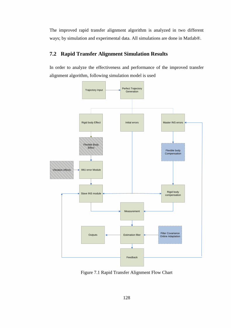
128

The improved rapid transfer alignment algorithm is analyzed in two different

ways; by simulation and experimental data. All simulations are done in Matlab®.

7.2 Rapid Transfer Alignment Simulation Results

In order to analyze the effectiveness and performance of the improved transfer

alignment algorithm, following simulation model is used

Trajectory Input Perfect Trajectory

Generation

Initial errorsRigid body Effect Master INS errors

Vibration effects

Flexible Body

Effect

IMU error Module

Slave INS moduleRigid body

compensation

Measurement

Feedback

Estimation filter

Flexible body

Compensation

Filter Covariance

Online AdaptationOutputs

Figure 7.1 Rapid Transfer Alignment Flow Chart

129

As it is already mentioned, there are two implementations. To see the performance

of each improvement, following simulation configurations are used;

1. Only high frequency vibration effects

2. Only low frequency flexible lever arm effects

Both vibration and flexibility effects are generated from the experimental data

shown in previous chapter.

Finally, all environmental effects are included with experimental flight data, and

the performance of the proposed implementations are tested

7.2.1 Simulation with Vibration Effects

The first step in the performance analysis is the inclusion of vibration effects to

the simulations as shown in Figure 7.1. With the inclusion of mechanical vibration

to the simulation, bias and noise shifts of inertial sensors are triggered. Also, the

high frequency components of launcher pod motion are also excited. The results

of simulations for vibration effects are given in Figure 7.2 to Figure 7.11 for

attitude (roll, pitch and yaw), gyro and accelerometer bias estimations. Note that

in this analysis, only vibration effects are included, dynamic misalignment is

analyzed in a separate case.

130

Figure 7.2 Estimation of Roll Attitude with Vibration Effects

Figure 7.3 Estimation of Roll Attitude with Vibration Effects

0 5 10 15 20 25 30-5

0

5

10

15

20 Roll Estimation Error

Time, s

Ro

ll E

rro

r, m

rad

Ideal TA

Real uncompensated TA

Compensated

20.5 21 21.5 22 22.5 23 23.5 24 24.5 25

-1

0

1

2

3

4

Roll Estimation Error

Time, s

Ro

ll E

rro

r, m

rad

Ideal TA


Compensated

131

Figure 7.4 Estimation of Pitch Attitude with Vibration Effects

Figure 7.5 Estimation of Azimuth Attitude with Vibration Effects

0 5 10 15 20 25 30-5

0

5

10

15

20 Pitch Estimation Error

Time, s

Ro

ll E

rro

r, m

rad

Ideal TA


Compensated

0 5 10 15 20 25 30-5

0

5

10

15

20 Azimuth Estimation Error

Time, s

Ro

ll E

rro

r, m

rad

Ideal TA


Compensated

132

Figure 7.6 Estimation of Azimuth Attitude with Vibration Effects

Figure 7.7 Estimation of X Accelerometer Bias with Vibration Effects

20.5 21 21.5 22 22.5 23 23.5 24 24.5 25 25.5

-1.5

-1

-0.5

0

0.5

1

1.5

2

2.5

Azimuth Estimation Error

Time, s

Ro

ll E

rro

r, m

rad

Ideal TA


Compensated

0 5 10 15 20 25 30-50

-40

-30

-20

-10

0

10

20

30 X Accelerometer Bias Estimation Error

Time, s

Bia

s E

rro

r, m

g

Ideal TA


Compensated

133

Figure 7.8 Estimation of Y Accelerometer Bias with Vibration Effects

Figure 7.9 Estimation of Z Accelerometer Bias with Vibration Effects

0 5 10 15 20 25 30-50

-45

-40

-35

-30

-25

-20

-15

-10

-5

0 Y Accelerometer Bias Estimation Error

Time, s

Bia

s E

rro

r, m

g

Ideal TA


Compensated

0 5 10 15 20 25 30-50

-40

-30

-20

-10

0

10

Z Accelerometer Bias Estimation Error

Time, s

Bia

s E

rro

r, m

g

Ideal TA


Compensated

134

Figure 7.10 Estimation of X Gyro Bias with Vibration Effects

Figure 7.11 Estimation of Y Gyro Bias with Vibration Effects

0 5 10 15 20 25 30-100

-50

0

50 X Gyro Bias Estimation Error

Time, s

Bia

s E

rro

r, d

eg

/hr

Ideal TA


Compensated

0 5 10 15 20 25 30-180

-160

-140

-120

-100

-80

-60

-40

-20

0

20 Y Gyro Bias Estimation Error

Time, s

Bia

s E

rro

r, d

eg

/hr

Ideal TA


Compensated

135

Figure 7.12 Estimation of Z Gyro Bias with Vibration Effects

The simulation results are summarized in Table 7.1

Table 7.1 Summary of Results - Vibration Effects

Ideal Uncompensated Compensated

Roll Estimation Error (mrad) 0.1 2.76 0.22

Pitch Estimation Error (mrad) 0.1 3.24 0.6

Azimuth Estimation Error (mrad) 0.1 0.95 0.14

X Gyro Bias Estimation Error 10 150 20

Y Gyro Bias Estimation Error 10 90 12

Z Gyro Bias Estimation Error 10 85 15

X Accelerometer Bias Estimation Error 1 10 3

Y Accelerometer Bias Estimation Error 1 12 4

Z Accelerometer Bias Estimation Error 1 9 4

From Figure 7.2 to Figure 7.12, the effects of uncompensated vibration effects are

easily seen. The vibration in the host platform directly affects gyro and

accelerometer bias and noise characteristics. As stated in Chapter 5, bias and noise

of an inertial sensor changes for a given vibration level. If this change is not

0 5 10 15 20 25 30-200

-150

-100

-50

0

50 Z Gyro Bias Estimation Error

Time, s

Bia

s E

rro

r, d

eg

/hr

Ideal TA


Compensated

136

compensated in rapid transfer alignment, especially bias estimation becomes

unusable.

Roll, pitch and yaw errors are also increased in the presence of vibration; while

the ideal estimation error was 0.1 mrad (without mechanical vibration effects),

the uncompensated errors increase up to 3 mrads. The adaptation of inertial noise

parameters of Kalman filter increases the transfer alignment algorithm

7.2.2 Simulation with Flexibility Effects

The second part of the performance analysis is done for dynamic misalignment

effects. Similar to previous part, dynamic misalignment data is generated and

integrated into the simulations, where mechanical vibrations are omitted. The

results are given in Figure 7.13 to Figure 7.19

Figure 7.13 Estimation of Pitch Attitude with Flexibility Effects

0 5 10 15 20 25 30-1.5

-1

-0.5

0

0.5

1

1.5

2x 10

-3 Pitch Estimation Error

Time, s

Ro

ll E

rro

r, d

eg

Ideal TA


State Augmentation

Neural Network

137

Figure 7.14 Estimation of Pitch Attitude with Flexibility Effects

Figure 7.15 Estimation of Roll Attitude with Flexibility Effects

0 5 10 15 20 25 30-1.5

-1

-0.5

0

0.5

1

1.5

2x 10


Time, s

Ro

ll E

rro

r, d

eg

Ideal TA


State Augmentation

Neural Network

0 5 10 15 20 25 30-1.5

-1

-0.5

0

0.5

1

1.5

2x 10

-3 Roll Estimation Error

Time, s

Ro

ll E

rro

r, d

eg

Ideal TA


State Augmentation

Neural Network

138

Figure 7.16 Estimation of Roll Attitude with Flexibility Effects

Figure 7.17 Estimation of X Gyro Bias with Flexibility Effects

22 22.5 23 23.5 24 24.5 25

-8

-6

-4

-2

0

2

4

6

8

10

12x 10


Time, s

Ro

ll E

rro

r, d

eg

Ideal TA


State Augmentation

Neural Network

0 5 10 15 20 25 30-100

-80

-60

-40

-20

0

20

40

60

80


Time, s

Bia

s E

rro

r, d

eg

/hr

Ideal TA


State Augmentation

Neural Network

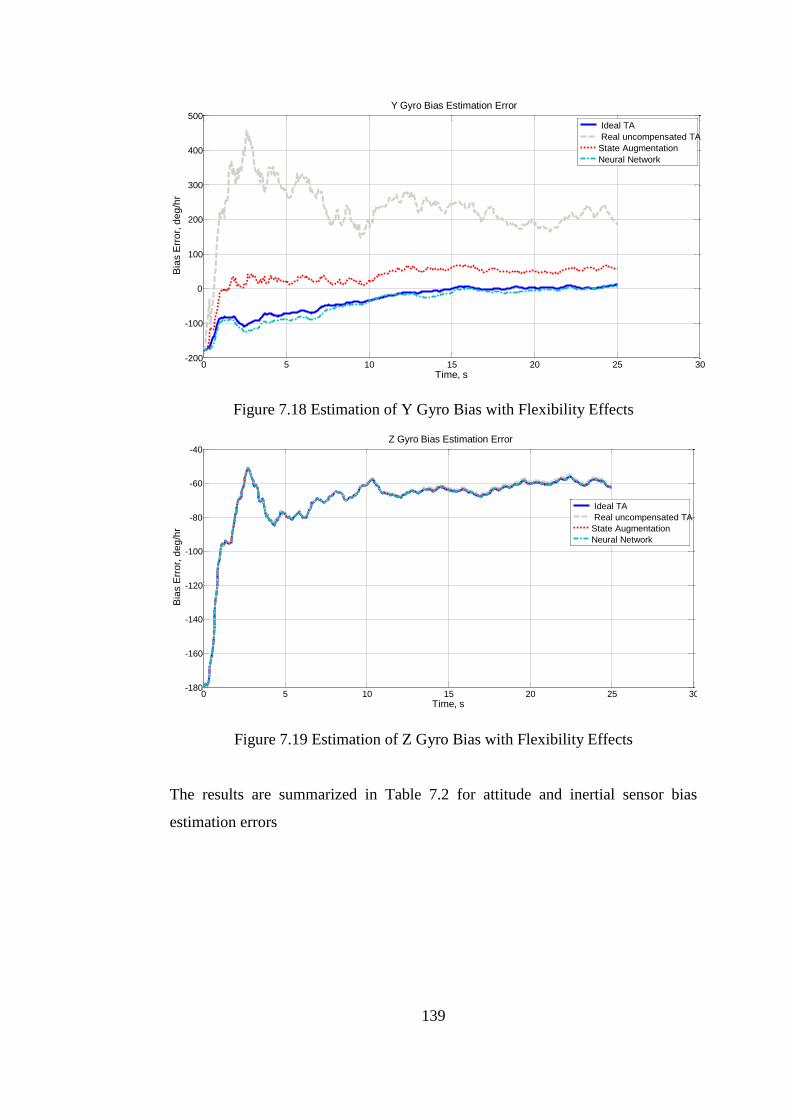
139

Figure 7.18 Estimation of Y Gyro Bias with Flexibility Effects

Figure 7.19 Estimation of Z Gyro Bias with Flexibility Effects

The results are summarized in Table 7.2 for attitude and inertial sensor bias

estimation errors

0 5 10 15 20 25 30-200

-100

0

100

200

300

400


Time, s

Bia

s E

rro

r, d

eg

/hr

Ideal TA


State Augmentation

Neural Network

0 5 10 15 20 25 30-180

-160

-140

-120

-100

-80

-60

-40 Z Gyro Bias Estimation Error

Time, s

Bia

s E

rro

r, d

eg

/hr

Ideal TA


State Augmentation

Neural Network

140

Table 7.2 Summary of Results - Flexibility Effects

Ideal Uncompensated State

Augmentation Neural

Network

Roll Estimation Error (mrad) 0.1 9.8 1.1 0.15

Pitch Estimation Error (mrad) 0.1 8.6 2.5 0.44

Azimuth Estimation Error (mrad) 0.1 0.2 0.14 0.15

X Gyro Bias Estimation Error 10 90 35 12

Y Gyro Bias Estimation Error 10 210 70 14

Z Gyro Bias Estimation Error 10 28 22 20

X Accelerometer Bias Estimation Error 1 10 3 2

Y Accelerometer Bias Estimation Error 1 12 3 3

Z Accelerometer Bias Estimation Error 1 9 4 2

As explained in Chapter 6, the dynamic misalignment is effective in roll and pitch

attitudes, where azimuth channel flexibility is negligible with respect to the

others. Roll and pitch errors are seriously increased, up to 10 mrads when there is

not compensation for dynamic misalignment. State augmentation reduces the error

in roll and pitch smaller than 2.5 mrads, where ANN performs superior and have a

performance near to the ideal transfer alignment case.

Inertial sensor bias estimations are also affected by the inclusion of dynamic

misalignment. The bias estimations of gyro and accelerometers are ten times

worse than the ideal transfer alignment. For state augmentation, the error between

ideal case is less than 3 mg for accelerometer, where the neural network performs

similar. In gyro bias estimation, neural network performs significantly better than

state augmentation.

In Figure 7.13 to Figure 7.18, it is easily seen that ANN compensation performing

near to the ideal rapid transfer alignment with no dynamic misalignment problem.

When there is no compensation of dynamic misalignment, roll and pitch attitude

estimation become very oscillatory. This oscillatory estimation directly effects the

related gyro bias estimations.

141

7.3 Rapid Transfer Alignment Experimental Results

The final step in the performance analysis in the transfer alignment improvements

is using experimental data instead of synthetically generated data. Recorded

Master, Slave and 2nd

master INS data is used in the analysis. The results are

given in Figure 7.20 to 7.28

Figure 7.20 Estimation of Pitch Attitude with Experimental Data

0 5 10 15 20 25 30-2

-1.5

-1

-0.5

0

0.5

1

1.5

2x 10


Time, s

Ro

ll E

rro

r, d

eg

Ideal TA


State Augmentation

Neural Network

4 4.5 5 5.5 6 6.5 7 7.5

-6

-5

-4

-3

-2

-1

0

1

2

3

4

x 10-4 Pitch Estimation Error

Time, s

Ro

ll E

rro

r, d

eg

Ideal TA


State Augmentation

Neural Network

142

Figure 7.21 Estimation of Roll Attitude with Experimental Data

0 5 10 15 20 25 30-1.5

-1

-0.5

0

0.5

1

1.5

2x 10


Time, s

Ro

ll E

rro

r, d

eg

Ideal TA


State Augmentation

Neural Network

23.5 24 24.5 25 25.5 26-6

-5

-4

-3

-2

-1

0

1

2

3

4

x 10-4 Roll Estimation Error

Time, s

Ro

ll E

rro

r, d

eg

Ideal TA


State Augmentation

Neural Network

143

Figure 7.22 Estimation of Azimuth Attitude with Experimental Data

0 5 10 15 20 25 30-5

0

5

10

15

20x 10

-4 Azimuth Estimation Error

Time, s

Ro

ll E

rro

r, d

eg

Ideal TA


State Augmentation

Neural Network

20.5 21 21.5 22 22.5 23 23.5 24 24.5 25

-2

-1

0

1

2

3

x 10-4 Azimuth Estimation Error

Time, s

Ro

ll E

rro

r, d

eg

Ideal TA


State Augmentation

Neural Network

144

Figure 7.23 Estimation of X Accelerometer Bias with Experimental Data

0 5 10 15 20 25 30-0.4

-0.35

-0.3

-0.25

-0.2

-0.15

-0.1

-0.05

0 X Accelerometer Bias Estimation Error

Time, s

Bia

s E

rro

r, m

/s2

Ideal TA


State Augmentation

Neural Network

21 21.5 22 22.5 23 23.5 24 24.5 25

-0.035

-0.03

-0.025

-0.02

-0.015

-0.01

X Accelerometer Bias Estimation Error

Time, s

Bia

s E

rro

r, m

/s2

Ideal TA


State Augmentation

Neural Network

145

Figure 7.24 Estimation of Y Accelerometer Bias with Experimental Data

0 5 10 15 20 25 30-0.4

-0.35

-0.3

-0.25

-0.2

-0.15

-0.1

-0.05

0 Y Accelerometer Bias Estimation Error

Time, s

Bia

s E

rro

r, m

/s2

Ideal TA


State Augmentation

Neural Network

11.2 11.3 11.4 11.5 11.6 11.7 11.8 11.9 12

-0.04

-0.035

-0.03

-0.025

-0.02

Y Accelerometer Bias Estimation Error

Time, s

Bia

s E

rro

r, m

/s2

Ideal TA


State Augmentation

Neural Network

146

Figure 7.25 Estimation of Z Accelerometer Bias with Experimental Data

0 5 10 15 20 25 30-0.4

-0.35

-0.3

-0.25

-0.2

-0.15

-0.1

-0.05

0 Z Accelerometer Bias Estimation Error

Time, s

Bia

s E

rror,

m/s

2

Ideal TA


State Augmentation

Neural Network

20.5 21 21.5 22 22.5 23 23.5 24 24.5 25

-0.035

-0.03

-0.025

-0.02

-0.015

-0.01

Z Accelerometer Bias Estimation Error

Time, s

Bia

s E

rror,

m/s

2

Ideal TA


State Augmentation

Neural Network

147

Figure 7.26 Estimation of X Gyro Bias with Experimental Data

Figure 7.27 Estimation of Y Gyro Bias with Experimental Data

0 5 10 15 20 25 30-100

-50

0

50

100


Time, s

Bia

s E

rro

r, d

eg

/hr

Ideal TA


State Augmentation

Neural Network

0 5 10 15 20 25 30-200

-100

0

100

200

300

400

500


Time, s

Bia

s E

rro

r, d

eg

/hr

Ideal TA


State Augmentation

Neural Network

148

Figure 7.28 Estimation of Z Gyro Bias with Experimental Data

Table 7.3 Summary of Results – Experiment

Uncompensated State

Augmentation Neural

Network

Roll Estimation Error (mrad) 14.4 2.3 1.2

Pitch Estimation Error (mrad) 15.8 2.4 0.84

Azimuth Estimation Error (mrad) 4.6 1.4 0.45

X Gyro Bias Estimation Error 220 48 25

Y Gyro Bias Estimation Error 170 54 38

Z Gyro Bias Estimation Error 185 57 26

X Accelerometer Bias Estimation Error 15 4 3

Y Accelerometer Bias Estimation Error 17 6 5

Z Accelerometer Bias Estimation Error 14 4 5

The real performance of the proposed implementations is shown in Table 7.3.

Both vibration and dynamic misalignment compensations are implemented. As in

the previous case, ANN performs better than state augmentation, but state

augmentation is also a good choice for dynamic misalignment compensation.

0 5 10 15 20 25 30-180

-160

-140

-120

-100

-80

-60

-40

-20

0

20 Z Gyro Bias Estimation Error

Time, s

Bia

s E

rror,

deg/h

r

Ideal TA


State Augmentation

Neural Network

149

As it is also seen from Figure 7.20 to 7.28, both state augmentation and neural

network have a distinguishable error compensation performance for

environmental effects. When combined with the adaptation of inertial and noise

parameters for flight vibration, both methods results in a very good accuracy. The

uncompensated roll, pitch and azimuth errors are about 15 mrads, where state

augmentation results in 2.4 mrad error and neural network has less than 1 mrad

error in the end of the transfer alignment. Also, the uncompensated transfer

alignment gives oscillatory results in attitude estimations, especially on roll and

pitch attitudes. Neural network performs two times better than state augmentation

in terms of steady state accuracy. Both methods have better convergence time

than uncompensated alignment. The uncompensated alignment have a

convergence time of at least 25-30 seconds, while both state augmentation and

neural network have 5-10 second convergence for bias estimations and 1-2

seconds for attitude estimations

The gyro bias estimations for uncompensated transfer alignment have an

unacceptable accuracy that cannot be used for online calibration. The gyros have a

bias repeatability of 100 deg/hr, while uncompensated transfer alignment has up

to 220 deg/hr estimation error. The state augmentation reduces the bias estimation

error to 50 deg/hr, while neural network further reduces it to 25 deg/hr.

The accelerometer bias estimations are also unacceptable for uncompensated

transfer alignment. The original bias repeatability of accelerometers is 10mg, but

the bias estimation error in transfer alignment is up to 17 mg. Both state

augmentation and neural network have similar estimation errors, approximately

5mg steady state error.

Briefly, both compensation methods have an important role for the rapid transfer

alignment under real environmental conditions. Especially bias estimations are

almost non-usable for online calibration for uncompensated alignment. Overall

performance of artificial neural network is obviously better than state

150

augmentation, but nevertheless state augmentation provides a significantly better

accuracy compared to the uncompensated transfer alignment

Vibration induced errors of inertial sensors have also an important role in the

transfer alignment. Vibration induced bias of gyros and accelerometers are pre-

calibrated, thus improving the bias estimation accuracy in the transfer alignment.

As stated in Chapter 5, the vibration induced errors are not permanent, when

vibration level is reduced, the vibration rectification will also be reduced. When

vibration induced bias is not taken into consideration in the transfer alignment, the

bias estimation will be faulty and will result in serious navigation performance

after launch phase

Vibration induced noise also affects the transfer alignment accuracy. Inertial

sensor noises are used in Kalman Filter process matrix, which directly affects the

steady state accuracy and convergence rate. Kalman filter is an optimal filter only

when the noise levels are entered correctly in the process noise matrix. In the

helicopter based transfer alignment, noises of gyros and accelerometers seriously

increases and this shift changes for different flight and loading configurations. In

the improved transfer alignment, accelerometer and gyro noises are adaptively

changed for different loading and flight conditions, thus optimizing the

performance of transfer alignment for all conditions.

151

CHAPTER 8

8 DISCUSSION and CONCLUSION

Almost all guided munitions require initial position, velocity and attitude data to

perform midcourse guidance. Initialization of an inertial navigation system is one

of the most challenging research area in this field, especially where the initialized

system is on the move. Transfer alignment is the process of aligning an inertial

navigation system with the aid of a higher accuracy navigation system. Transfer

alignment is done by parameter matching between master and slave INS through

Kalman Filter. In transfer alignment, primary goal is to align the slave INS, but

slave INS can also be pre-launch calibrated, thus increasing the midcourse

performance of the guided munition.

In an ideal environment, the final alignment accuracy of the slave inertial

navigation system depends only on the accuracy of the master INS. In real

alignment case, the transferred alignment information is degraded by host

platform’s structure. In the ideal transfer alignment, the velocity and attitude

information from master navigation system is directly transferred to the slave INS

by an only rigid body coordinate transformation as the attitude between master

and slave INS is perfectly known. In the real case, this coordinate transformation

has uncertainties due to the dynamic behavior of the slave INS location. For most

of the guided munitions, the launcher has high and low frequency motions with

respect to the main navigation system. For aircrafts, high frequency motion,

152

namely mechanical vibrations have negligible effect, but the low frequency

motion, the wing distortion severely degrades the attitude accuracy of the

alignment. In order to align the guided munition under these effects, the attitude

information is usually not used in the parameter matching phase of the transfer

alignment. Attitude is used only in the one shot transfer phase, but in the

estimation phase, only velocity data is transferred, becoming velocity matching

transfer alignment. In velocity matching, the uncertainties due to vibration and

wing distortion is eliminated, thus a higher accuracy can be achieved with respect

to the attitude matching. With these uncertainties present in the alignment

environment, velocity matching is more robust and stable. But, observability of

the transfer alignment is dependent to the input motion of the system, i.e. the

maneuver of the host platform. While velocity is direct observable, attitude and

related inertial sensor errors are indirect observables. In order to obtain complete

observability of the main navigation states and inertial sensor errors, the platform

needs to make specific maneuvers. These maneuvers are s or c shaped maneuvers

which takes a time of 1-3 minutes depending on the platform. Also, this type of

maneuvers makes a tactical constraint to the pilot of the platform.

In order to align the slave INS within a smaller time interval, attitude information

should be included in the parameter matching. Rapid transfer alignment is the

parameter matching method where both velocity and attitude information is used

in the estimation phase.

Main goal of this thesis is to design a rapid transfer alignment algorithm with

proper compensation of the dynamic relative motion of the launcher. The

improvements are in three different parts;

Stochastic observability analysis

Vibration compensation

Flexibility compensation

153

Generally, observability of states in transfer alignment or in integrated navigation

system is done by classical deterministic observability approach; by checking the

rank of the observability matrix. This approach has two disadvantages;

Effects of stochastic components, noises are not included in the

observability analysis

The degree of observability is not analyzed.

Observability analysis is used for two purposes; determining an optimum

maneuver for the platform and selecting proper system states. Two different

observability methods are used; eigenvalue and covariance matrix approach. In

the eigenvalue approach, the eigenvalues of the system states with respect to time

is analyzed, whereas in the covariance matrix approach, the eigenvalues of the

related variance states are analyzed. Both methods investigate the degree of

observability with noise effects. In order to see the convergence rate of each state,

detailed Monte Carlo simulations should be done, where the observability and

convergence characteristics are heuristically analyzed. The proposed methods

provide an easier way for this. Stochastic observability is also important in

system state selection. A system can be seen as fully observable, as the related

observability matrix has full rank, but certain states cannot be estimated. The

reason of this unobservability is the noise characteristics of the states. In Chapter

4, the observability characteristics of the system states of rapid transfer alignment

are demonstrated for different maneuvers. The main parameters, velocity and

attitude have a distinctly higher degree of observability with respect to inertial

sensor biases regardless of the maneuver performed. There is only slight change

in the degree of observability of velocity and attitude for different maneuvers,

which means that for very rapid transfer alignment, the completion of a tactical

maneuver is not necessary. It is showed that in rapid transfer alignment, a

maneuver is required to increase the observability of inertial sensor error

estimations. It is also showed that the scale factor errors are always unobservable

regardless of the maneuver. This unobservability arises from the nature of the

Slave INS sensors, MEMS gyros and accelerometers have such a noise profile

154

that is masks the scale factor error. The observability analysis summarizes that an

s or c shaped maneuver is sufficient to obtain complete high rate observability.

Also, depending on observability analysis, the scale factor errors are omitted from

transfer alignment, thus reducing the computational load of the algorithm.

High frequency mechanical vibration in a helicopter launched guided munition is

serious problem. In most of guided munitions, MEMS type inertial sensors are

used. Especially, MEMS gyros have a distinct sensitivity to the vibrations in the

platform as they are basically Coriolis Vibratory Gyros. In the literature, vibration

sensitivity of the MEMS sensors are analyzed in detail to be used in any

compensation algorithm. Chapter 5 is divided into two sections, characterization

of the vibration environment and investigation of inertial sensor performance

under these vibrations. In the beginning of the chapter, effects of vibration to the

transfer alignment is shown, the steady state and convergence rate is severely

degraded. The characterization of the vibration environment is done by two

different ways; from military standards and experimental data. The military

standard for environmental considerations, Mil-Std-810F gives vibration profile

for almost all type of platforms, but these profiles are over safe. The main purpose

of this military standard is to define environmental conditions and profiles for

operational durability, i.e. a munition or its component which can stand the profile

defined in Mil-Std-810F is certain to work in the related platform. In order to

make a more realistic vibration profile, experimental data is collected for different

flight conditions. It is shown that vibration amplitude directly depends on the

cruise speed of the helicopter. In the second part of the thesis, vibration effects on

inertial sensor performance are shown. Main error parameters that are affected

form vibration are bias and noise. It is known that any vibration rectification in

bias and noise depends on the amplitude of vibration, not frequency. This is a

result of the specific resonant frequency of the MEMS sensors, about 14 kHz. The

variation of bias and noise is determined by ground test with a vibration table. As

it is shown, vibration profile of the launcher pod in the helicopter depends on

velocity and loading configuration. Thus vibration rectification of bias and noise

155

can be handled in transfer alignment as the velocity and loading configuration is

known.

Dynamic misalignment, namely flexibility between master and slave INS is

known to be a problem mostly in aircraft launched munitions, but it also appears

as a serious effect in helicopters. As in the vibration characterization and

compensation, Chapter 6 is divided into two parts as characterization and

modeling. In order to characterize the dynamic misalignment, real flight data is

collected. In data acquisition, a second high accuracy navigation grade inertial

navigation system is implemented in the launcher pod, thus the attitude between

master INS and launcher pod can be accurately tracked. With these experimental

data, two different modeling approaches are considered; state augmentation and

artificial neural network. In state augmentation, a Markov model is used to online

compensate the dynamic misalignment in the transfer alignment. The model order

and related parameters are determined by the real flight data and augmented into

the Kalman filter. The second method, artificial neural network is trained by the

experimental flight data in an offline manner. The offline trained ANN is used to

compensate the dynamic misalignment with respect to the platform velocity and

loading configuration. When two methods are compared for their estimation

performance, it is easily seen that ANN approach performs better. ANN is the

optimum compensation method for dynamic misalignment whenever detailed data

of launcher pod dynamics is available. State augmentation also provides a usable

estimation of dynamic misalignment. When there is limited offline data, state

augmentation should be used for compensation.

In Chapter 7, performance of the proposed implementations is tested in transfer

alignment. In order to test each implementation; three different test method is

used;

Only Vibration Effects

Only Flexibility Effects

All effects with complete experimental data.

156

In first two cases, vibration and flexibility data is generated from the previously

collected data, shown in Chapter 5 and 6.

Characterization and modeling of inertial sensors’ vibration sensitivity is shown to

be very effective in the simulations. Without the vibration effect compensation,

the accuracy of attitude estimation is severely degraded, whereas the inertial

sensor bias estimation nearly becomes unusable without any compensation. With

the experimental data, the bias and noise rectification for a given platform velocity

and loading configuration can be found.

Both state augmentation and artificial neural network is shown to be effective in

dynamic misalignment compensation. ANN performs better than state

augmentation. When no dynamic misalignment compensation is done in the

transfer alignment, the dynamic behavior of the launcher pod is directly seen in

the estimation results; attitude estimations have a distinct oscillatory error, and

gyro bias estimation are so degraded that they become unusable.

Finally, in order to see the integrated performance, the proposed implementations

are tested in real flight environment with experimental flight records. The results

for;

No Compensation

Inertial sensor vibration compensation + state augmentation

Inertial sensor vibration compensation + artificial neural network

The results are similar to the previous analysis; if there is not any compensation

for relative motion of the launcher pod, the alignment performance is severely

degraded, also in flight calibration is not possible. Artificial neural network and

state augmentation performs similar, where ANN is slightly better than Markov

model

157

Briefly, the main contributions of this thesis are;

Stochastic Observability analysis methods for maneuver and state

selection in Rapid Transfer Alignment are derived, where the degree of

observability of each state can be analyzed.

Vibration sensitivity of MEMS inertial sensors is characterized and

modeled in the Transfer Alignment. Bias and noise shifts for a given flight

and launch configuration is shown.

Dynamic misalignment between master and slave INS is characterized and

modeled into the rapid transfer alignment algorithm. Two different

methods are derived and tested with experimental data.

For future work, following studies can be done;

An analytical model the launcher pod’s dynamic motion can be derived.

The results of analytical and estimated dynamic misalignment can be

compared

An online training method for ANN can be designed, thus the offline work

load can be reduced.

158

REFERENCES

1. Titterton, D. H. and Weston, J. L., Strapdown Inertial Navigation

Technology 2nd ed., Peter Peregrinus Ltd., London, (2004).

2. Rogers, R. M. (2000). Applied Mathematics in Integrated Navigation

Systems, AIAA Education Series,Reston, Virginia.

3. Groves, P. D., “Optimising the Transfer Alignment of Weapon INS”, The

Journal of Navigation, 56: 323-335 (2003).

4. Lim,Y.C., Lyou, “An Error Compensation Method for Transfer

Alignment”, 0-7803-7101-1/01, 2001 IEEE

5. Yüksel, Y., Design and Analysis of Transfer Alignment Algorithms. ,M.Sc

Thesis,METU, Ankara.

6. Klotz, H. A. and Derbak, C. B., “GPS-Aided Navigation and Unaided

Navigation on the Joint Direct Attack Munition”, IEEE, 0-7803-4330-

1/98, 412-419 (1998).

7. Kain, J. E. and Cloutier, J. R., “Rapid Transfer Alignment for Tactical

Weapon Applications”, AIAA, AIAA-89-3581-CP, 1290-1300 (1989).

8. Shortelle, K. J. and Graham, W. R., “F-16 Flight Tests of a Rapid Transfer

Alignment Precedure”, IEEE, 0-7803-4330-1/98, 379-386 (1998)

9. Schneider, A. M., “Kalman Filter Formulations for Transfer Alignment of

Strapdown Inertial Units”, Journal of the Institute of Navigation, 30 (1):

72-89(1983).

10. Rogers, R. M., “Weapon IMU Transfer Alignment Using Aircraft Position

from Actual Flight Tests”, IEEE, 0-7803-3085-4/96, 328-335 (1996)

11. Ross, C. C. and Elbert, T. F., “A Transfer Alignment Algorithm Study

Based on Actual Flight Test Data from a Tactical Air-to-Ground Weapon

Launch”, IEEE, 0-7803-1435-2/94, 431-438 (1994).

159

12. Rogers, R. M., “Low Dynamic IMU Alignment”, IEEE, 0-7803-4330-

1/98,272-279 (1998).

13. Rogers, R. M., “Comparison of Inertial Navigation System Error Models

in Application to IMU Transfer Alignment”, AIAA, AIAA-97-3599, 686-

695 (1997).

14. Hallingstad, O., “Design of A Kalman Filter for Transfer Alignment”,

AGARD, Kalman Filter Integration of Modern Guidance and Navigation

Systems, 1-14 (1989).

15. Spalding, K., “An Efficient Rapid Transfer Alignment Filter”, AIAA,

AIAA-92- 4598-CP, 1276-1286 (1992).

16. Graham, W. and Shortelle, K. (1995). “Advanced Transfer Alignment for

Inertial Navigators (A-Train)” Proceedings of the Institute of Navigation

National Technical Meeting 1995.

17. Shortelle, K. and Graham, W., “Advanced Alignment Concepts for

Precision- Guided Weapons”, Proc Natl ION, (1995).

18. Graham, W. R., Shortelle, K. J. and Rabourn, C. (1998). “Rapid

Alignment Prototype (RAP) Flight Test Demonstration”, Proceedings of

the Institute of Navigation National Technical Meeting 1998.

19. Shortelle, K. J. and Graham, W. R. (1998).” F-16 Flight Tests of a Rapid

Transfer Alignment Procedure”. Proceedings of IEEE Position, Location

And Navigation Symposium 1998.

20. Groves, P. D. (1999). “Transfer Alignment Using an Integrated INS/GPS

as the Reference”, Proceedings of the Institute of Navigation 55th Annual

Meeting.

21. Groves, P. D. and Haddock, J. C., “An All-Purpose Rapid Transfer

Alignment Algorithm Set”, Institute of Navigation National Technical

Meeting, California, (2001).

22. Groves, P. D. and Haddock, J. C. (2001). “An All-purpose Rapid Transfer

Alignment Algorithm” Set. Proceedings of the Institute of Navigation

National Technical Meeting 2001.

160

23. Groves, P. D., Wilson, G. G. and Mather, C. J., “Robust Rapid Transfer

Alignment with an INS/GPS Reference”, Institute of Navigation National

Technical Meeting, California,1-11 (2002)

24. Wendel, J., Metzger, J. and Trommer, G. F., “Rapid Transfer Alignment in

The Presence of Time Correlated Measurement and System Noise”, AIAA

Guidance, Navigation and Control Conference and Exhibit, Rhode Island,

1-12 (2004).

25. Koifman, M. and Bar-Itzhack, I. Y., “Inertial Navigation System Aided

byAircraft Dynamics”, IEEE Transactions on Control Systems

Technology, 7 (4):487-493 (1999).

26. Pehlivanoğlu, A.G, Uçaklardaki Esnemelerin Aktarım Yönlendirme

Performansı Üzerindeki Etkileri,., Gazi Üniversitesi 2009

27. Kaiser, J. and Beck, G., “ Vital Advanced Inertial Network”, IEEE, 0-

7803-4330-1/98, 61-68 (1998).

28. Carlson, N. A., Kelley, R. T. and Berning, S. L., “Differential Inertial

Filter for Dynamic Sensor Alignment”, Proc Natl ION, 341-351 (1994).

29. Wendel, J. and Trommer, G. (2001). „Impact of Mechanical Vibrations on

the Performance of Integrated Navigation Systems and On Optimal IMU

Specification”. Proceedings of the Institute of Navigation 57th Annual

Meeting.

30. Wendel, J. and Trommer, G. (2002). „IMU Performance Requirement

Assessments for GPS/INS Missile Navigation Systems”. Proceedings of

the Institute of Navigation 58th Annual Meeting.

31. Goshen-Meskin, D. and Bar-Itzhack, I. Y., “Observability Analysis of

Piece- Wise Constant Systems - Part I: Theory”, IEEE Transactions on

Aerospace and Electronic Systems, 28 (4): 1056-1067 (1992).

32. Goshen-Meskin, D. and Bar-Itzhack, I. Y., “Observability Analysis of

Piece- Wise Constant Systems - Part II: Application to Inertial Navigation

In-Flight Alignment”, IEEE Transactions on Aerospace and Electronic

Systems, 28 (4): 1068-1075 (1992).

33. Wang, J., Lee, H. K., Hewitson, S. and Lee H. - K., “Influence of

Dynamics and Trajectory on Integrated GPS/INS Navigation

161

Performance”, Journal of Global Positioning Systems, 2 (2): 109-116

(2003).

34. Hong, S., Chun, S., Kwon, S.H., Lee, M.H., “Observability Measures and

Their Application to GPS/INS”, IEEE Trans. On Vehicular Technology,

Vol. 57, No.1, January 2008

35. Chung, D., Park, C.G. and Lee, J.G., “Observability Analysis of

Strapdown Inertial Navigation System Using Lyapunov Transformation”

36. Gao, W. and Sun, F. “Comparison of INS Transfer Alignment through

Observability Analysis” , 0-7803-9454-2/06, 2006 IEEE

37. Hao, Y. , Xiong, Z. and Xiond B., “Estimation Error of INS Transfer

Alignment through Observability Analysis”, 0-7803-9395-3, 2006 IEEE

38. Bageshwar, V., Gebre-Egziabher, D., Garrard, W.L., Georgiou T.T.,

“Stochastic Observability Test for Discrete Time Kalman Filter”, Journal

of Guidance, Control and Dynamics, Vol 32, No. 4, July- August 2009

39. Gelb, A. Applied Optimal Estimation, M.I.T. Press, Cambridge,

Massachusetts, 1974

40. Maybeck, P.S., Stochastic Models Estimation and Control, Vol. 1,

Academic Press (1979).

41. Ham, F.M., Brown, R.G., “Observability, Eigenvalues and Kalman

Filtering”, 0018-9251/83/0300-0269, 1983 IEEE

42. Porat, B., Bar-Itzhack, I., “Effect of Acceleration Switching During INS

In-Flight Alignment”, Journal of Guidance, Control and dynamics, Vol. 4.,

No:4 July – August 1981

43. Porat, B., Bar-Itzhack, I., “Azimuth Observability Enhancement During

Inertial Navigation System In- Flight Alignment”, Journal of Guidance,

Control and dynamics, Vol. 3., No:4 July – August 1980

44. O. Tekinalp and M. Ozemre, “Artificial Neural Networks for Transfer

Alignment and Calibration of Inertial Navigation Systems”, AIAA 2001-

4406.

162

45. Huang, Y.W and Chiang, K.W. (2007). “The AI Based Compensators for

a Rapid and Accurate Alignment Procedure : An Open Loop Approach”,

ION GNSS 2007

46. Kaygısız, H.B. Intelligent Methods for Dynamic Analysis and Navigation

of Autonomous Land Vehicles, Ph.D. Thesis, METU 2004

47. Jwo, D.J., Huang, H.C., Huang, J., “A Neural Network Aided Adaptive

Kalman Filtering Approach for GPS Navigation”, ION GPS/GNSS 2003

48. Xiyuan, C., “Modeling Random Gyro Drift By Time Series Neural

Networks and by Traditional Method”, 0-7803-7702-8/03 2003 IEEE

49. IEEE-528-2001, IEEE Standard for Inertial Sensor Terminology.

50. Mil-STD-810-F Test Method Standard For Environmental Engineering

Considerations and Laboratory Tests,

51. Karimi, M., “Finite Sample Criteria for Autoregressive Model Order

Selection”, Journal of Science and Technology, Transaction B., Vol.31

No.B3, pp 329-344, 2007

52. Burshtein, D., Weinstein E, “Some Relations Between the Various

Criteria for Autoregressive Model Order Determination”, IEEE

Transactions on Acoustics, Speech and Signal Processing, Vol. 3, No 4,

1985

53. Khorsidi S., Karimi M., “Optimal autoregressive model order selection in

the sense of prediction error”, Proceeding of ICEE 2010, 978-1-4244-

6760-0/10

54. Paulson, A., Swope G., “Autoregressive Process Order Selection Via

Model Critical Methods”, IEEE Journal of Oceanic Engineering, Vol. 12,

No. 1, 1997

55. Broersen, P., Wensink E., “On Finite Sample Theory for Autoregressive

Model Order Selection”, IEEE Transactions on Signal Processing Vol. 41,

No. 1, 1993

56. Chen, C., Davis, R., Brockwell, P., Bai, Z., “Order Determination for

Autoregressive Processes using Resampling Methods”, Statistica

Sinica,Vol 3, pp 481-500, 1993

163

57. Widrow B., Lehr M.A., 1990, “30 years of adaptive neural networks:

perceptron, madaline and backpropagation”, Proceedings of the IEEE, vol.

78, no. 9, September 1990, pp. 1415-1442

58. Yu X.H., Chen G.A., “Efficient backpropagation learning using optimal

learning rate and momentum”, Neural Networks, vol. 10, no. 3, 1997,

pp.517-527

59. Yu X.H., Chen G.A., Cheng S.X., “Dynamic learning rate optimization of

the backpropagation algortihm”, IEEE Transactions on Neural Networks,

vol. 6, no. 3, 1995, pp. 669-677

164

APPENDIX A

A DERIVATION OF INS EQUATIONS

In an inertial navigation system, the platform’s position, velocity and attitude with

respect to Earth in inertial axis is required. The basic navigation mechanization

equation is given by [1,2];

2

2

i

d rf

dt (A.1)

And

2

2

i

d ra g

dt (A.2)

where

f: Rigid body acceleration in inertial axis frame

a: Accelerometer measurements

g: gravitational acceleration

165

r: position vector

Remember that accelerometers are unable to sense gravitational acceleration

directly

Coriolis equation is included in order to find the velocity relative to Earth

ie

i e

dr drr

dt dt (A.3)

Differentiating A.3 and including e

e

drv

dt ;

2

2

( ) e ie

i ii

dv d rd r

dt dt dt

(A.4)

2

2( ) e

ie e ie ie

ii

dvd rv r

dt dt (A.5)

where the angular rotation rate of Earth is assumed to be constant, i.e. 0ied

dt

Rearranging equations A.4 and A.5;

( ) neie e ie ie

i

dva v r g

dt (A.6)

Where;

na : Inertial sensor acceleration measurement in navigation frame

166

ie exv : Transport rate

( )ie iex xr : Centrifugal acceleration due to the the rotational rate of Earth, which

cannot be separate the gravitational acceleration. The sum of this centrifugal

acceleration and gravitational acceleration is known as plumb-up gravity

( )p ie ieg g x xr (A.7)

Navigation (local geographic) axis frame is required to navigate all around the

Earth. In navigation frame, position is given in latitude, longitude and altitude,

whereas velocity is given in North-East-Down components.

In navigation frame, ground speed is denoted as n

ev . The rate of change of ground

speed with respect to local geographic frame written in inertial frame is given by;

( ) e eie en e

n i

dv dvv

dt dt (A.8)

Substituting e

i

dv

dt;

(2. ) neie en e p

n

dva v g

dt (A.9)

which can be rearranged as;

. (2. ) n n b n

e b ie en e pv C a v g (A.10)

167

n

bC : Body to navigation frame transformation direction cosine matrix.

Direction cosine matrix is mechanized as follows;

( )n n b

b b nbC C

b

nb :The angular rotation rate of a body with respect to the navigation frame

b

nb : Skew symmetric matrix form of b

nb

b

nb can also be written as the measured body rates (b

ib ) and estimates of the

navigation frame rotation rate components ( in ie en ) ;

.( )b b n n n

nb ib b ie enC (A.11)

Remember that local geographic frame is required to have a continuous rotation as

the navigated platform moves in Earth in order to have an x axis parallel to Earth

Surface. This rotation rate of the local geographic frame is also known as

transport rate, expressed by (A.12);

[ /( ) /( ) .tan( ) /( )]n

en E e N n E eV R h V R h V L R h (A.12)

The coordinate transformation between navigation and earth frames can be

expressed by;

( )e e n

n n enC C (A.13)

168

The dynamic change of position states; latitude, longitude and altitude is given

by;

N

N

VL

R h (A.14)

sec( )

E

N

V Ll

R h (A.15)

Dh V (A.16)

169

APPENDIX B

B DERIVATION OF INS ERROR EQUATIONS

In this section, error propagation model of a full inertial navigation system is

derived. The related error equations are expressed in navigation axis frame [1, 22

and 23].

B.1 Attitude Errors

The attitude between the navigation and erroneous navigation) axis frame is

given asas;

ˆ .n n n

b b bC C C (B.1)

where

ˆ n

bC : Ideal navigation frame

n

bC : Real navigation frema

n

bC : Attitude transformation matrix between ideal and real navigation frame

Remember that the attitude kinematics is given as;

170

.( ) ( ). n n b n n

b b ib in bC C C (B.2)

Differentiating this equation;

.( ) .( ) ( ). ( ). n n b n b n n n n

b b ib b ib in b in bC C C C C (B.3)

where attitude difference between ideal and real navigation frame is assumed to

small, n

bC is stated as a vector;

( ). n n n

b bC C (B.5)

n : Attitude error vector

Taking this equation’s derivative with respect to time;

( ). ( ). n n n n n

b b bC C C (B.5)

Include n

bC

( ). ( ).( .( ) ( ). ) n n n n n b n n

b b b ib in bC C C C (B.6)

Equating both equations;

.( ) .( ) ( ). ( ).

( ). ( ).( .( ) ( ). )

n b n b n n n n

b ib b ib in b in b

n n n n b n n

b b ib in b

C C C C

C C C

(B.7)

And solving for attitude error vector rate

( ). .( ) ( ).( ).

( ).( ). ( ).

n n n b n n n

b b ib in b

n n n n n

in b in b

C C C

C C

(B.8)

171

Multiplying on the right by the inverse ofn

bC ;

( ) .( )( ) ( ).( ) ( ).( ) ( ) n n b n T n n n n n

b ib b in in inC C (B.9)

. n n b n n n

b ib in inC (B.10)

Remember that n

en and n

ie are given by;

. tan( )[ ]

n TN NEen

E N E

V V LV

R h R h R h (B.11)

and

[ cos( ) 0 sin( )]n T

ie L L (B.12)

n

in is defined by;

n n n

in ie en (B.13)

n n n

in ie en (B.14)

where

.n e e

ie n ieC (B.15)

Note that e

ie does not change with respect to time.

Position error is given by n

172

.n n e e

ie n iexC (B.16)

n : Position Error given in navigation frame

Rearranging the equation results in;

n n n n n

ie ie iex x (B.17)

Alternatively, n

en and n

ie is given by;

2

2 2

( )

. tan( ) . tan( ) .

( ) ( )(cos( ))

E E

E E

n N Nen

N N

N N N

E E E

V V h

R h R h

V V h

R h R h

V L V L h V

R h R h R h L

(B.18)

[ sin( ) 0 cos( ) ]n T

ie L L L L (B.19)

B.2 Velocity Errors

Note that velocity mechanization equation is expressed as;

. (2. ) n n b n

e b ie en e pv C a v g (B.20)

Differentiating this equation;

173

. .

(2. ) (2. )

n n b n b

e b b

n n

ie en e ie en e p

v C a C a

v v g

(B.21)

Including attitude error, n

bC and neglecting second order effects results in;

( . ) . (2. )

(2. )

n n b n n b n n n n

e b b e ie en

n n n

ie en e p

v C a C a v

v g

(B.22)

B.3 Position Errors

Position mechanization equation is given as;

( )e e n

n n enC C (B.23)

Differentiating this equation

( ) ( ) e e n e n

n n en n enC C C (B.24)

Defining;

( )e e n

n nC C (B.25)

n : Position error vector

Differentiating with respect to time;

( ) ( ) e e n e n

n n nC C C (B.26)

174

Rearranging;

( )( ) ( ) e e n n e n

n n en nC C C (B.27)

Equating these equations

( )( ) ( ) ( ) ( ) e n n e n e n e n

n en n n en n enC C C C (B.29)

Solving for n

( ) ( ) ( ) ( )( ) e n e n e n e n n

n n en n en n enC C C C (B.29)

Multiply on the left by the inverse of e

nC

( ) ( )( ) ( ) ( )( ) n n n n n n

en en en (B.30)

Rearranging;

n n n n

en enx (B.31)

Altitude error is given by taking derivative with respect to time

Dh V (B.32)

Dh V (B.33)

Alternatively, position errors in latitude and longitude can be expressed as

follows;

175

/( ) . /( ) N n N nL V R h V h R h (B.34)

.sec( ) /( ) .sec( ).tan( ). /( )

.sec( ). /( )

E e E e

E e

l V L R h V L L L R h

V L h R h

(B.35)

176

APPENDIX C

C ARTIFICIAL NEURAL NETWORKS

Artificial Neural Network (ANN) is an alternative solution methodused in various

fields of engineering such as estimation, system identification, guidance, control,

optimization, classification, pattern recognition etc. A neural networks consists of

several neurons which are computing components connected to other neurons in

several layers [44-48, 57, 58].

ANN is inspired by biological neural systems; basically they are simplified model

of the brain. The fundamental element of ANN is a neuron as in the case of a

biological neural network. ANN is composed of many neurons that work in co-

operation in order to complete the necessary function. Biological neuron and a

simple neuron model for ANN is shown in Figure C.1 and Figure C.2;

Figure C.1 Biological Neuron Model [57]

177

Figure C.2 Neuron Model [57]

Every neuron has a multi input-output structure. Main property of an ANN is its

learning property,that is it can adapt itself to the dynamics of the system and

environment by the neurons connected to each other. [58]

Main property of ANN is the ability to learn; they figure out the way to perform

the required function by themselves and they determine their function based on

sample inputs.

Inputs to the neuron are separately weighted. The output is the addition process

with a nonlinear activation function, in other words the output of a neuron is a

function of weighted sum of the inputs.

The basic neuron is defined by;

1

N

i i

i

u w x

(C.1)

And

( )y f u (C.2)

x: Inputs for neuron

w: Weight for synapses

u: Neuron activation

178

: Threshold

y: Output of the neuron

f(): Activation function

Taking w0= and threshold input as x0=-1, equation B.2 is rearranged as;

0

( )N

i i

i

y f w x

(C.3)

There are different kinds of activation functions for different applications [45].

Most common ones are linear, hard limit and log sigmoid functions. In

classification applications, hard limit activation is used, which simply makes a

quantization of the output to 0 or 1. In linear filter design, linear function is

preferred. In back propagation algorithms, sigmoid function is used. The sigmoid

function is given as;

( ) 1/ (1 )uf u e (C.4)

As it is seen from equation B.4, main difference between sigmoid and other

activation functions is that the sigmoid function is differentiable, which is

fundamental for learning in ANN.

Multilayer perceptron (MLP) with feed forward property is one of the most

common neural network type used in engineering. The multilayer feed forward

neural network structures with proper layers (input, output and hidden layers) are

accepted as general approximation functions.

In multilayer feed forward networks, there are multiple layers; additional hidden

layers are present between input and output layers. Also, the information in

multilayer feed forward network proceeds in one direction, each layers output is

the input for the next one. There may be more than one hidden layer.

179

Main function of multilayer perceptron is to make an approximation and

estimation for a given input and output profile [44, 45].

Figure C.3 Multilayer Feedforward Network Architecture [57]

In the output layer, the weighted sum of all layers’ output is processed by a

nonlinear activation function, [ ]s

jf

1

[ ] [ ] [ ]

[ ] [ ] [ 1]

0

( )

s

s s s

j j j

ns s s

j ji i

i

o f u

u w o

(C.5)

[ ]s

jiw : Synaptic weight for multiplication of the jth

neuron of the sth

layer multiplies

the ith

output from preceding layer [ 1]s

io . Each weighting is tuned by the training

in the ANN learning phase.

ns: Number of neurons present in sth

layer

Back propagation learning is the training and learning process in multilayer feed

forward neural networks. With the learning process, ANN can adapt itself for

input output mapping. Back propagation is a supervised form of training. The

fundamental of back propagation is based on ANN’s error minimization.

180

Figure C.4 ANN with back propogation [57]

In back propagation algorithm [57,58], input processed to the layers of the ANN

and resulting output is compared to the sample output. This comparison results in

the output error, which is back propagated in reverse; from output to the input

layer in order to tune the synaptic weights with a proper learning algorithm, thus

minimizing the output error. This back propagation procedure is done in a loop

unless the final output error is below the specified level.

Back propagation can either be done offline or online. In offline training,

predetermined or recorded input output mapping is used, whereas real time input

outputs are used in online training.

One of the most common methods for training is to use gradient descent algorithm

for error minimizations. Error function is given by;

2 2

2 2

1 1

1( ) ( )

2

n n

p jp jp jp

j j

E d y e

(C.6)

181

p: The learning step

djp : Desired output of ANN

yjp : Actual output of ANN

For over all learning process, error function is expressed as;

2

2

0...

( )p p jp jp

p p j n

E E d y

(C.7)

n2 : Number of neurons in the output layer

In the learning process, the changing of each weighting is given by;

[ ]

[ ], 0

ps

ji s

ji

Ew

w

(C.8)

: Learning parameter.

Delta weighting in the output layer is expressed as;

[2] [2] [1]

ji j iw o (C.9)

Where

[2]

[2]

[2]( )

jp

j jp jp

j

fd y

u

(C.10)

For the hidden layer,

[1] [1] [0]

ji j iw o (C.11)

Where

182

2[1]

[2] [2] [2]

[1]1

njp

j k kj

kj

fw

u

(C.12)

Have been obtained.

Gradient descent is a common and simple method used in many back propagation

applications, but it has some important disadvantages such s learning rate

sensitivity, slow convergence and lower accuracy with respect to the other

methods such simulated annealing, Levenberg Marquardt.

183

APPENDIX D

D KALMAN FILTERING

Kalman filter is the most common integration and estimation method used in

inertial navigation systems, where navigation states (position, velocity and

attitude) should be updated in order to obtain a bounded, usable solution. Kalman

filter is the most common estimation method used to update inertial navigation

data with redundant information from external sources, GPS, magnetometer,

terrain data, or like the case in this thesis, master INS. There are different types of

Kalman filter for different system applications, such as Extended Kalman Filter,

Unscented Kalman Filter etc. which are all practical to be applied in real time.

The basic Kalman Filter is a linear estimation algorithm. For most of the inertial

navigation system applications, linearized error equations of navigation states are

used in linear Kalman filter as the navigation states themselves are highly

nonlinear. The navigation error states should be bounded in small numerical

interval for valid linearity assumption.

Kalman filter uses state space model of the estimated and measured systems. In

the remaining parts of Appendix C, the fundamentals of the discrete time Kalman

filter is derived and explained in detail. [26, 27, 28, 29].

184

Main problems and questions for the inertial navigation data are listed as follows;

Navigation errors should be corrected in motion so that navigation data is

useful even with limited initial navigation data

Measurements from various aiding system (GPS, altimeter, magnetometer

etc.) with different time intervals should be optimally combined

Covariance of the navigation states should be estimated to see the

confidence level of the noisy system.

All navigation and inertial sensor states should be estimated even if only

some of the states are observed, that is the system is a reduced order

observer.

The Kalman filter is the optimum solution for the above problems. The flow of

this minimum variance linear estimation algorithm is as follows;

Kalman filter is initialized by ox̂ , the statistical estimates for the initial

navigation error states, P(t0), the covariance matrix of the estimated states,

and Q0, the process noise covariance.

States ox̂ and their covariance P(t0) are propagated to the measurement

update

Measurement and the related innovation term is calculated

Kalman gain is calculated in order to obtain minimum mean square error

estimate

Estimates of navigation states are calculated by measurement zk through

Kalman gain

With the convergence of the filter, all states (both navigation errors and inertial

sensor calibration parameters) are estimated on the move. Also, the uncertainty of

each state is found. With each measurement update, covariance values are

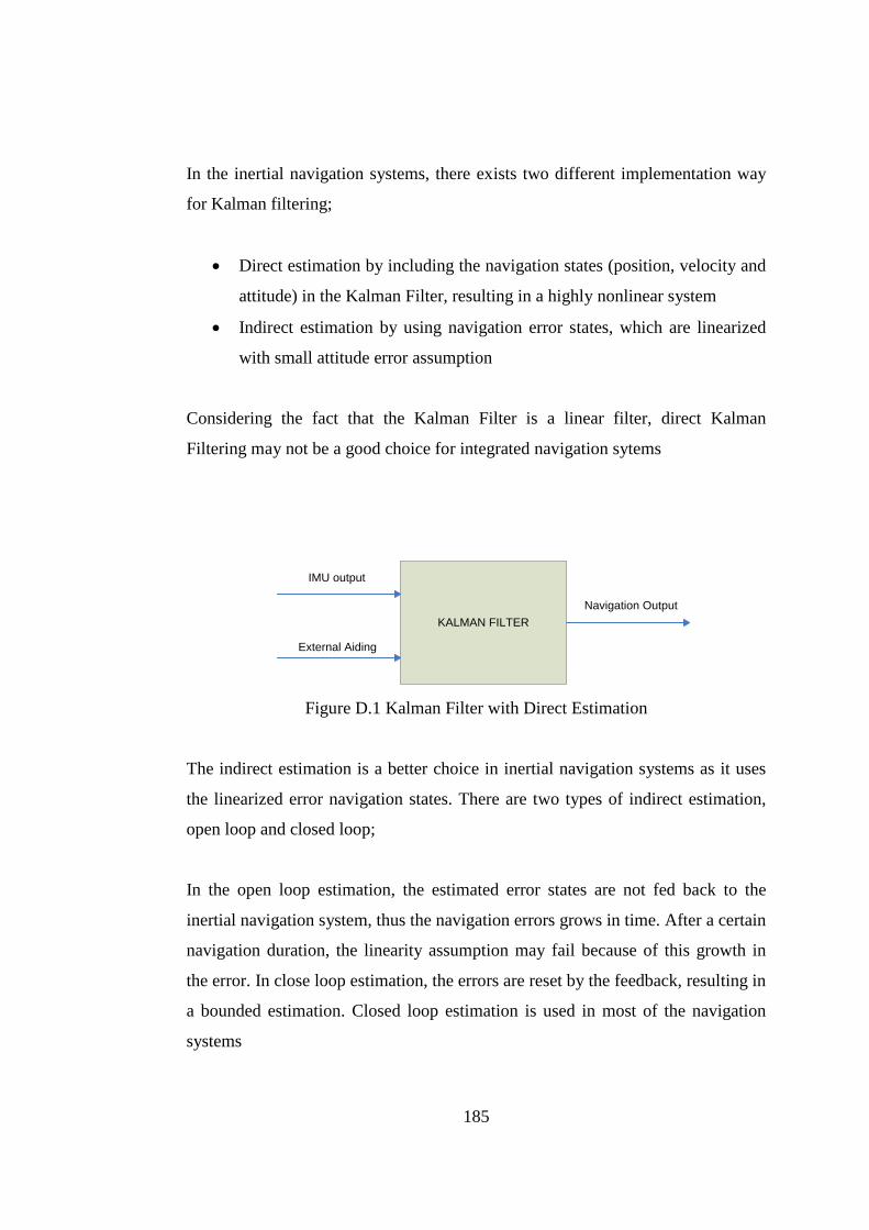
185

In the inertial navigation systems, there exists two different implementation way

for Kalman filtering;

Direct estimation by including the navigation states (position, velocity and

attitude) in the Kalman Filter, resulting in a highly nonlinear system

Indirect estimation by using navigation error states, which are linearized

with small attitude error assumption

Considering the fact that the Kalman Filter is a linear filter, direct Kalman

Filtering may not be a good choice for integrated navigation sytems

KALMAN FILTER

IMU output

External Aiding

Navigation Output

Figure D.1 Kalman Filter with Direct Estimation

The indirect estimation is a better choice in inertial navigation systems as it uses

the linearized error navigation states. There are two types of indirect estimation,

open loop and closed loop;

In the open loop estimation, the estimated error states are not fed back to the

inertial navigation system, thus the navigation errors grows in time. After a certain

navigation duration, the linearity assumption may fail because of this growth in

the error. In close loop estimation, the errors are reset by the feedback, resulting in

a bounded estimation. Closed loop estimation is used in most of the navigation

systems

186

KALMAN FILTER

INS

EXTERNAL AIDING



errors

Figure D.2 Indirect Open Loop Kalman Filter

KALMAN FILTER

INS

EXTERNAL AIDING



errors

Figure D.3 Indirect Close Loop Kalman Filter

Discrete Time Kalman Filter equations are given in table D.1

187

Table D.1 Discrete Time Kalman Filter [26]

Noisy system dynamics equation in

discrete time

k 1 k k kx A x w

Process Noise covariance T

k k kE(w w ) Q

Measurement equation in discrete

time

k k k kz H x v

Measurement noise covariance T

k k kE(v v ) R

A priori estimate of the states '

k k k k kˆ ˆx ( ) K x ( ) K z

'

k k kK (I K H )

A posteriori estimate of the states

k k k k k kˆ ˆ ˆx ( ) x ( ) K [z H x ( )]

T T 1

k k k k k k kK P ( )H [H P ( )H R ]

Propagated covariance matrix with

measurements

k k k kP ( ) (I K H )P ( )

1 1 T 1

k k k k kP ( ) P ( ) H R H

Time update Equations

k 1 k kˆ ˆx ( ) A x ( )

T

k 1 k k k k

T

k k k

P ( ) A P ( )A Q

Q E(w w )

188

APPENDIX E

E INERTIAL SENSOR SPECIFICATIONS

Table E.1 Slave INS Performance Specifications

PERFORMANCE (1)

Gyros

Measurement Range > 500 deg/sec

Dynamic Bandwidth 50 Hz

Scale Factor Repeatability < 1000 ppm

Nonlinearity < 1000 ppm

Bias Repeatability < 100 deg/hr

Axis Misalignment 3 mrad

Random Walk 1 deg/hr

g Sensitivity < 100 deg/hr/g

Accelerometers

Measurement Range 30g




Bias Repeatability < 10 mg

Axis Misalignment 3 mrad

Random Walk 0.5 m/s/hr

Start-up Time 100 ms

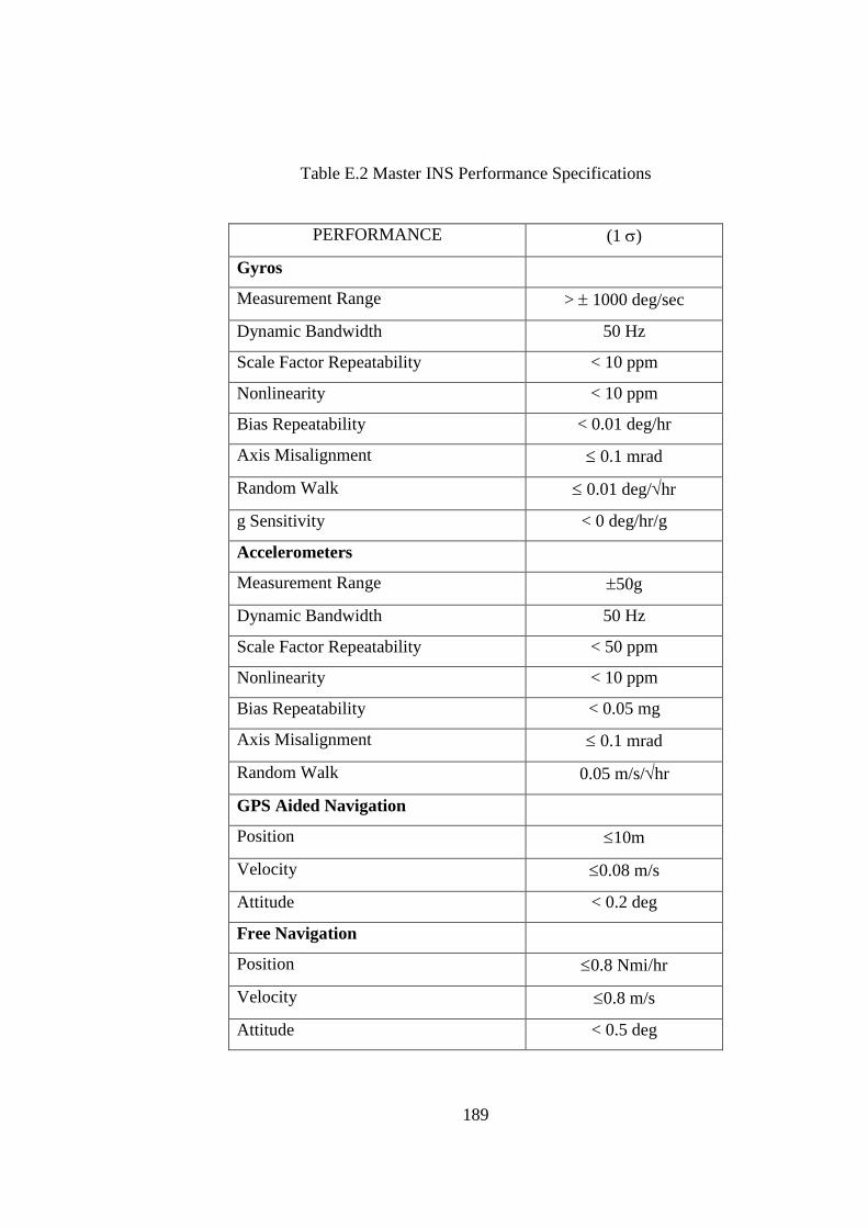
189

Table E.2 Master INS Performance Specifications

PERFORMANCE (1)

Gyros

Measurement Range > 1000 deg/sec




Bias Repeatability < 0.01 deg/hr

Axis Misalignment 0.1 mrad

Random Walk 0.01 deg/hr

g Sensitivity < 0 deg/hr/g

Accelerometers

Measurement Range 50g




Bias Repeatability < 0.05 mg

Axis Misalignment 0.1 mrad

Random Walk 0.05 m/s/hr

GPS Aided Navigation

Position 10m

Velocity 0.08 m/s

Attitude < 0.2 deg

Free Navigation

Position 0.8 Nmi/hr

Velocity 0.8 m/s

Attitude < 0.5 deg

190

APPENDIX F

F SIMULINK MODELS FOR RAPID TRANSFER

ALIGNMENT

F.1 INPUT FILE FOR ALGORITHM

dt=0.05;

acc1BiasInstabErrTC_db = 0 ; % 1 / a_xb bias

instability error time constant (1/s)

acc1BiasInstabErrTC = acc1BiasInstabErrTC_db;

acc2BiasInstabErrTC_db =0 ; % 1 / a_yb_IMU bias



acc3BiasInstabErrTC_db = 0 ; % 1 / a_zb_IMU bias



acc1SFInstabErrTC_db = 0 ; % 1 / a_xb scale

factor instability error time constant (1/s)

acc1SFInstabErrTC = acc1SFInstabErrTC_db;

acc2SFInstabErrTC_db = 0 ; % 1 / a_yb_IMU scale



191

acc3SFInstabErrTC_db =0 ; % 1 / a_zb_IMU scale



gyr1BiasInstabErrTC_db = 0 ; % 1 / p_IMU bias


gyr1BiasInstabErrTC = gyr1BiasInstabErrTC_db;

gyr2BiasInstabErrTC_db = 0 ; % 1 / q_IMU bias



gyr3BiasInstabErrTC_db = 0 ; % 1 / r_IMU bias



gyr1SFInstabErrTC_db = 0 ; % 1 / p_IMU scale


gyr1SFInstabErrTC = gyr1SFInstabErrTC_db;

gyr2SFInstabErrTC_db =0 ; % 1 / q_IMU scale



gyr3SFInstabErrTC_db = 0 ; % 1 / r_IMU scale



vxSigma_db = 25 ; % std of Vx (m/s) ( std :

standard deviation )

vxSigma = vxSigma_db;

vxVar = vxSigma^2;

vySigma_db = 25 ; % std of Vy (m/s)

vySigma = vySigma_db;

vyVar = vySigma^2;

vzSigma_db = 25 ; % std of Vz (m/s)

192

vzSigma = vzSigma_db;

vzVar = vzSigma^2;

phiSigma_db = 15 ; % std of phi (deg)

phiSigma = phiSigma_db * pi/180; % (deg --> rad)

phiVar = phiSigma^2;

thetaSigma_db = 15 ; % std of theta (deg)

thetaSigma = thetaSigma_db * pi/180; % (deg --> rad)

thetaVar = thetaSigma^2;

psiSigma_db = 15 ; % std of psi (deg)

psiSigma = psiSigma_db * pi/180; % (deg --> rad)

psiVar = psiSigma^2;

% accBiasSigma_db = 20 ; % std of accelerometer

bias repeatability error (g)

accBiasSigma_db = 40e-3; %20; %0;

accBiasSigma = accBiasSigma_db * 9.81; % (g --> m/s^2)

accBiasVar = accBiasSigma^2;

% accSFSigma_db = 10000; % std of

accelerometer scale factor repeatability error (ppm)

accSFSigma_db = 2000; %0;

accSFSigma = accSFSigma_db * 10^-6 ; % (ppm --> non

dimension)

accSFVar = accSFSigma^2;

% gyrBiasSigma_db = 150 ; % std of gyro bias

repeatability error (deg/hr)

gyrBiasSigma_db = 150*1.2; %125; % 0;

193

gyrBiasSigma = gyrBiasSigma_db * (pi/180) * (1/3600) ; % (deg/hr

--> rad/s)

gyrBiasVar = gyrBiasSigma^2;

% gyrSFSigma_db = 10000 ; % std of gyro scale

factor repeatability error (ppm)

gyrSFSigma_db = 2000; %1000; % 0;

gyrSFSigma = gyrSFSigma_db * 10^-6; % (ppm --> non

dimension)

gyrSFVar = gyrSFSigma^2;

% accNoiseSigma_db = 0.01 ; % std of

accelerometer noise (g)

% accNoiseSigma = accNoiseSigma_db * 9.81 ; % (g -->

m/s^2)

accNoiseSigma =0.01 * sqrt(1/dt);

accNoiseVar = accNoiseSigma^2;

gyrNoiseSigma_db =0.02*0.15; %0.001 ; % std of

gyro noise (deg/s)

gyrNoiseSigma = gyrNoiseSigma_db * pi/180 * sqrt(1/dt) ; %

(deg --> rad)

gyrNoiseVar = gyrNoiseSigma^2;

accBiasNoiseSigma_db = 0 ; % std of

accelerometer bias noise (g)

accBiasNoiseSigma = accBiasNoiseSigma_db * 9.81;

accBiasNoiseVar = accBiasNoiseSigma^2;

accSFNoiseSigma_db = 0 ; % std of acclerometer

scale factor noise (ppm)

194

accSFNoiseSigma = accSFNoiseSigma_db * 10e-6; % (ppm --

> non dimension)

accSFNoiseVar = accSFNoiseSigma^2;

gyrBiasNoiseSigma_db = 0; % std of gyro bias

noise (deg/hr)

gyrBiasNoiseSigma = gyrBiasNoiseSigma_db * (pi/180) * (1/3600); %

(deg/hr --> rad/s)

gyrBiasNoiseVar = gyrBiasNoiseSigma^2;

gyrSFNoiseSigma_db = 0 ; % std of gyro scale

factor noise (ppm)

gyrSFNoiseSigma = gyrSFNoiseSigma_db * 10e-6 ; % (ppm --

> non dimension)

gyrSFNoiseVar = gyrSFNoiseSigma^2;

gravityDeviationSigma_db = 0 ; % std of gravitational

acceleration anomaly (mg)

gravityDeviationSigma = gravityDeviationSigma_db * 10e-3 * 9.81; %

(mg --> m/s^2)

gravityDeviationVar = gravityDeviationSigma^2;

pltVelNoiseSigma_db = 0.001*10 ; %0.001 % std of

noise in platform velocity data (m/s)

pltVelNoiseSigma = pltVelNoiseSigma_db ;

pltVelNoiseVar = pltVelNoiseSigma^2;

pltEulerNoiseSigma_db = 0.0001*200*2; %0.0001 %

std of noise in platform euler angle data (deg)

pltEulerNoiseSigma = pltEulerNoiseSigma_db * pi/180 ; % (deg -->

rad)

pltEulerNoiseVar = pltEulerNoiseSigma^2;

195

rLncPltNoiseSigma_db = 0.05; %0.001 ; % std of

variation in platform INS - pod distance (m)

rLncPltNoiseSigma = rLncPltNoiseSigma_db ;

rLncPltNoiseVar = rLncPltNoiseSigma^2;

pltAngVelNoiseSigma_db = 0.0001*10 ; % std of noise

in platform angular velocity data (deg/s)

pltAngVelNoiseSigma = pltAngVelNoiseSigma_db * pi/180; % (deg

--> rad)

pltAngVelNoiseVar = pltAngVelNoiseSigma^2;

latencyLimit1 = 0.02 ;

latencyLimit2 = 0.05 ;

dtTfralignEst = 0.05;

tfralignDelay = 0;

velocity_sigma_limit_db = 1 ; % limit for std of

velocity estimation (m/s)

velocityVarLimit = velocity_sigma_limit_db^2 ;

euler_sigma_limit_db = 0.1 ; % limit for std or euler

angle estimation (deg)

euler_sigma_limit = euler_sigma_limit_db * pi/180;

eulerVarLimit = euler_sigma_limit^2 ;

aXbBiasSigmaLimit_db = 0.01; %g %variance

degerinin 1/5i...

aXbBiasSigmaLimit = aXbBiasSigmaLimit_db * 9.81;

aXbBiasVarLimit = aXbBiasSigmaLimit^2;

aYbBiasSigmaLimit_db = 0.01;

196

aYbBiasSigmaLimit = aYbBiasSigmaLimit_db * 9.81;

aYbBiasVarLimit = aYbBiasSigmaLimit^2;

aZbBiasSigmaLimit_db = 0.01;

aZbBiasSigmaLimit = aZbBiasSigmaLimit_db * 9.81;

aZbBiasVarLimit = aZbBiasSigmaLimit^2;

aXbSFSigmaLimit_db = 1000; %ppm

aXbSFSigmaLimit = aXbSFSigmaLimit_db * 10e-6;

aXbSFVarLimit = aXbSFSigmaLimit^2;

aYbSFSigmaLimit_db = 1000;

aYbSFSigmaLimit = aYbSFSigmaLimit_db * 10e-6;

aYbSFVarLimit = aYbSFSigmaLimit^2;

aZbSFSigmaLimit_db = 1000 ;

aZbSFSigmaLimit = aZbSFSigmaLimit_db * 10e-6;

aZbSFVarLimit = aZbSFSigmaLimit^2;

pBiasSigmaLimit_db = 3; %deg/hr

pBiasSigmaLimit = pBiasSigmaLimit_db * pi/180 * 1/3600;

pBiasVarLimit = pBiasSigmaLimit^2;

qBiasSigmaLimit_db = 3; %deg/hr

qBiasSigmaLimit = qBiasSigmaLimit_db * pi/180 * 1/3600;

qBiasVarLimit = qBiasSigmaLimit^2;

rBiasSigmaLimit_db = 3; %deg/hr

rBiasSigmaLimit = rBiasSigmaLimit_db * pi/180 * 1/3600;

rBiasVarLimit = rBiasSigmaLimit^2;

pSFSigmaLimit_db = 1000; %ppm

pSFSigmaLimit = pSFSigmaLimit_db * 10e-6;

pSFVarLimit = pSFSigmaLimit^2;

qSFSigmaLimit_db = 1000; %ppm

qSFSigmaLimit = qSFSigmaLimit_db * 10e-6;

197

qSFVarLimit = qSFSigmaLimit^2;

rSFSigmaLimit_db = 1000; %ppm

rSFSigmaLimit = rSFSigmaLimit_db * 10e-6;

rSFVarLimit = rSFSigmaLimit^2;

% aXbBiasVarLimit = accBiasVar/5;

%

% aYbBiasVarLimit = accBiasVar/5;

% aZbBiasVarLimit = accBiasVar/5;

%

% aXbSFVarLimit = accSFVar/5;

% aYbSFVarLimit = accSFVar/5;

% aZbSFVarLimit = accSFVar/5;

%

% pBiasVarLimit = gyrBiasVar/5;

% qBiasVarLimit = gyrBiasVar/5;

% rBiasVarLimit = gyrBiasVar/5;

%

% pSFVarLimit = gyrSFVar/5;

% qSFVarLimit = gyrSFVar/5;

% rSFVarLimit = gyrSFVar/5;

deltaHPltSLLimit_db = 15; %m

deltaHPltSLLimit = deltaHPltSLLimit_db;

deltaHPltGLLimit_db = 15; %m

deltaHPltGLLimit = deltaHPltGLLimit_db;

deltaLatPltLimit_db = 2 ; %arc sec

deltaLatPltLimit = deltaLatPltLimit_db /3600 * pi/180 ;

deltaLonPltLimit_db = 2; %arc sec

deltaLonPltLimit = deltaLonPltLimit_db /3600 * pi/180 ;

biasAccXUpper = 0;

198

SFAccXUpper = 0;

biasAccYUpper = 0;

SFAccYUpper = 0;

biasAccZUpper = 0;

SFAccZUpper = 0;

biasGyrXUpper = 0;

SFGyrXUpper = 0;

biasGyrYUpper = 0;

SFGyrYUpper = 0;

biasGyrZUpper = 0;

SFGyrZUpper = 0;

199

F.2 SIMULINK BLOCKS

Figure F.1 Main Rapid Transfer Alignment Algorithm

a_

ve

l_p

lta

_ve

l_fu

ze

a_

ve

l_e

rrR

esh

ap

e

Re

sha

pe

Eule

r_plt

Eu

ler_

fuze

V_plt

INS

Ve

locity

Ve

cto

r

va

rian

ce

Ve

cto

r

INS

Ve

locity

Ve

cto

rErr

INS

An

gu

larP

ositio

nV

ecto

rErr

bia

s

SF

OU

TP

UT

phi

the

ta

psi

C_

b2

n

phi

the

ta

psi

C_

b2

n

C(e

w)_

0

w_

AO

B

a_A

OB

Vm

_e

_F

B1

C_

b2

n

eule

r

INS

_p

lt

C(e

w)_

0

w_

AO

B

a_A

OB

INS

Ve

locity

Ve

cto

rUp

da

te

INS

An

gu

larP

ositio

nV

ecto

rUp

da

te

Vm

_e

_F

B1

C_

b2

n

eule

r

INS

_m

issile

[a_

AO

B_

fuze

]

[Eu

ler_

fuze

]

[w_

AO

B_

plt]

[Eu

ler_

plt]

[V_

plt]

[va

rian

ce

Ve

cto

r]

[INS

An

gu

larP

ositio

nV

ecto

rErr]

[INS

Ve

locity

Ve

cto

rErr]

[CB

NM

atrix

]

[gyrZ

SF

Up

da

te]

[gyrZ

Bia

sUp

da

te]

[gyrY

SF

Up

da

te]

[gyrY

Bia

sUp

da

te]

[gyrX

SF

Up

da

te]

[gyrX

Bia

sUp

da

te]

[accZ

SF

Up

da

te]

[w_

AO

B_

fuze

]

[accZ

Bia

sUp

da

te]

[accY

SF

Up

da

te]

[accY

Bia

sUp

da

te]

[a_

AO

B_

plt]

[V_

plt2

]

[INS

An

gu

larP

ositio

nV

ecto

rUp

da

te]

[INS

Ve

locity

Ve

cto

rUp

da

te]

[accX

SF

Up

da

te]

[accX

Bia

sUp

da

te]

[INS

Ve

locity

Ve

cto

r]

[w_

AO

B_

plt]

[V_

plt]

[Eu

ler_

plt]

[INS

Ve

locity

Ve

cto

r]

[INS

An

gu

larP

ositio

nV

ecto

rUp

da

te]

[INS

An

gu

larP

ositio

nV

ecto

rUp

da

te]

[INS

Ve

locity

Ve

cto

rUp

da

te]

[V_

plt]

[w_

AO

B_

fuze

]

[Eu

ler_

plt]

[gyrZ

SF

Up

da

te]

[gyrY

SF

Up

da

te]

[gyrX

SF

Up

da

te]

[accZ

SF

Up

da

te]

[accY

SF

Up

da

te]

[accX

SF

Up

da

te]

[gyrZ

Bia

sUp

da

te]

[gyrY

Bia

sUp

da

te]

[a_

AO

B_

fuze

]

[gyrX

Bia

sUp

da

te]

[accZ

Bia

sUp

da

te]

[INS

Ve

locity

Ve

cto

r]

[accY

Bia

sUp

da

te]

[INS

Ve

locity

Ve

cto

rErr]

[va

rian

ce

Ve

cto

r]

[V_

plt]

[INS

An

gu

larP

ositio

nV

ecto

rErr]

[INS

Ve

locity

Ve

cto

rUp

da

te]

[INS

Ve

locity

Ve

cto

rUp

da

te]

[V_

plt2

]

[INS

Ve

locity

Ve

cto

rUp

da

te]

[INS

An

gu

larP

ositio

nV

ecto

rErr]

[Eu

ler_

fuze

]

[accX

Bia

sUp

da

te]

[CB

NM

atrix

]

[w_

AO

B_

plt]

[a_

AO

B_

plt]

[w_

AO

B_

fuze

]

[a_

AO

B_

fuze

]

[INS

Ve

locity

Ve

cto

rErr]

a_

ref

w_

ref

w_

imu

a_

imu

vP

Plt

vQ

Plt

vR

Plt

vV

No

rthP

lt

vV

Ea

stP

lt

vV

Do

wn

Plt

vP

hiP

lt

vT

he

taP

lt

vA

ziPlt

INS

Ve

loctiy

Ve

cto

r

cb

nM

atrix

RL

ncP

lt

DC

ML

ncP

lt

aXb

IMU

aY

bIM

U

aZ

bIM

U

IMU

An

gu

larV

elo

city

Ve

cto

r

gIN

S

INS

Ve

locity

Ve

cto

rErr

INS

An

gu

larP

ositio

nV

ecto

rErr

accX

Bia

sS

FU

pd

ate

accY

Bia

sS

FU

pd

ate

accZ

Bia

sS

FU

pd

ate

gy

rXB

iasS

FU

pd

ate

gy

rYB

iasS

FU

pd

ate

gy

rZB

iasS

FU

pd

ate

va

rian

ce

Ve

cto

r

Estim

atio

n A

nd

Me

asu

rem

en

t

[0;0

;0]

eu

ler0

g

eye

(3)

(0 0 0)

200

Figure F.2 Missile INS Algorithm

Figure F.3 Host INS Algorithm

3

euler

2

C_b2n

1

Vm_e_FB1

u

ICy

1

z

u

ICy

1

z

phi

theta

psi

C_b2n

Initial DCM2

Cb2n_fuze

Cb2n_fuzeMatrix

Multiply

Matrix

Multiply

C_b2n

phi

theta

psi

DCM2Euler1

[0 0 g]'

dt

Vm_w0-1

[0 0 0]'

C_b2n_1

wib

win

C_b2n

Attitude Update1

5

INSAngularPositionVectorUpdate

4

INSVelocityVectorUpdate

3

a_AOB

2

w_AOB

1

C(ew)_0

phi

theta

psi

3

euler

2

C_b2n

1

Vm_e_FB1

u

ICy

1

z

u

ICy

1

z

Cb2n_plt

Cb2n_plt

Cb2n_pltMatrix

Multiply

Matrix

Multiply

C_b2n

phi

theta

psi

DCM2Euler1

[0 0 g]'

dt

Vm_w0

[0 0 0]'

C_b2n_1

wib

win

C_b2n

Attitude Update1

3

a_AOB

2

w_AOB

1

C(ew)_0

psi

theta

phi

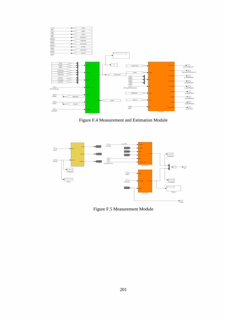
201

Figure F.4 Measurement and Estimation Module

Figure F.5 Measurement Module

9

varianceVector

8

gyrZBiasSFUpdate

7

gyrYBiasSFUpdate

6

gyrXBiasSFUpdate

5

accZBiasSFUpdate

4

accYBiasSFUpdate

3

accXBiasSFUpdate

2

INSAngularPositionVectorErr

1

INSVelocityVectorErr

a_Ypqr_plt

V_plt_NED

Euler_plt

ins_v elocity _v ector

C_B2N

rLncPlt

DCM_plt2lnc

Yk

C_N2plt

Measurement

[CBNMatrix]

[measVector]

[vAziPlt]

[vThetaPlt]

[vPhiPlt]

[rLncPlt]

[vVDownPlt]

[vVEastPlt]

[vVNorthPlt]

[vRPlt]

[vQPlt]

[vPPlt]

[cPltN]

[CBNMatrix]

[measVector]

[rLncPlt]

[vAziPlt]

[vThetaPlt]

[vPhiPlt]

[vVDownPlt]

[vVEastPlt]

[vVNorthPlt]

[vRPlt]

[vQPlt]

[vPPlt]

[cPltN]

Yk

C_N2plt

sf ib

wib

C_B2N

rLncPlt

g_ins

v elocity _corr

euler_corr

a_xb_update

a_y b_update

a_zb_update

p_update

q_update

r_update

v arianceVector

Estimation

18

gINS

17

IMUAngularVelocityVector

16

aZbIMU

15

aYbIMU

14

aXbIMU

13

DCMLncPlt

12

RLncPlt

11

cbnMatrix

10

INSVeloctiyVector

9

vAziPlt

8

vThetaPlt

7

vPhiPlt

6

vVDownPlt

5

vVEastPlt

4

vVNorthPlt

3

vRPlt

2

vQPlt

1

vPPlt

V_plt_NED

2

C_N2plt

1

Yk

[w_plt]

[w_plt]

C_B2N

DCM_plt2lnc

C_N2plt

Euler_dif f

Z2 Calculation

V_plt_NED

C_NED2N

C_N2plt

w_plt

rLncPlt

ins_v elocity _v ector

v el_dif f

Z1 Calculation

a_euler_plt

To Workspace3

a_euler_diff

To Workspace2

a_vel_diff

To Workspace1

U( : )

pqr_plt

Euler_plt

w_plt

C_N2plt

C_NED2N

Local Parameters Calculation

Display1

Display

[C_N2plt]

[C_N2plt]

[C_N2plt]

[C_NED2N]

[C_NED2N]

7

DCM_plt2lnc

6

rLncPlt

5

C_B2N

4

ins_velocity_vector

3

Euler_plt

2

V_plt_NED

1

pqr_plt

202

Figure F.6 Attitude Measurement Module

Figure F.7 Velocity Measurement Module

Figure F.8 Kalman Filter Module

3

C_NED2N

2

C_N2plt

1

w_plt

uT

a b

Skew-Symmetric form

uT

phi

theta

psi

C_b2n

Initial DCM

0

Gain1

Matrix

Multiply

C_plt_2_N Calculation

a b

C_NED2N Calculation

2

Euler_plt

1

pqr_plt

v _Az_plt

w_plt

C_NED2plt

C_NED2N

1

vel_diff

Matrix

Multiply

Matrix

Multiply

Matrix

Multiply

V_plt_N

uT

6

ins_velocity_vector

5

rLncPlt

4

w_plt

3

C_N2plt

2

C_NED2N

1

V_plt_NED

(wxr)_N

V_plt_N

(wxr)_plt

C_plt2N

1

Euler_diff

U( : )U( : )

Reshape

Matrix

Multiply

3

C_N2plt

2

DCM_plt2lnc

1

C_B2N

(1,3)

(3,2)

CB2N_dif f

9

varianceVector

8

r_update

7

q_update

6

p_update

5

a_zb_update

4

a_yb_update

3

a_xb_update

2

euler_corr

1

velocity_corr

X

P

g_ins

v elocity _corr

euler_corr

a_xb_update

a_y b_update

a_zb_update

p_update

q_update

r_update

v ariance_v ector

Module Outputs

Yk

C_N2plt

sf ib

wib

C_B2N

rLncPlt

X_state

P_cov ariance

Kalman

7

g_ins

6

rLncPlt

5

C_B2N

4

wib

3

sfib

2

C_N2plt

1

Yk

203

Figure F.9 Kalman Filter Updates Module

Figure F.10 Output Module

2

P_covariance

1

X_state

instability

v ariance

-C-

dt

[X]

[P]

[R]

[Q]

[Gm]

[H]

[PHI]

[G]

u

ICy

1

z

X kIk

a_X

a_P

a_P_prediction

a_P_state

a_R

a_P_state_diag

a_X_state_diag

a_P_prediction_diag

a_X_state

a_X_prediction1

a_G

a_H

a_Gm

a_PHI

a_Q

a_X_prediction

a_K

PHI

X kIk

X k+1Ik

StatePrediction

Yk

H

X k+1Ik

K

X k+1Ik+1

StateCorrection

Reshape

Reshape

u

ICy

1

z

P kIk

Memory

H

Gm

P k+1Ik

R

K

KalmanGain

dt

v ariance

instability

C_N2plt

sf ib

wib

C_B2N

rLncPlt

G

H

Gm

PHI

Q

R

P

X

INIT

[P]

[H]

[H]

[Gm]

[H]

[PHI]

[Q]

[X]

[R]

[G]

[PHI]

A D

A D

PHI

P kIk

G

Q

P k+1Ik

CovariancePrediction

K

P k+1Ik

H

P k+1Ik+1

CovarianceCorrection

6

rLncPlt

5

C_B2N

4

wib

3

sfib

2

C_N2plt

1

Yk

5

varianceVector1

stdVector

bias

SF

accXbias

accYbias

accZbias

gy rXbias

gy rYbias

gy rZbias

accXSF

accYSF

accZSF

gy rXSF

gy rYSF

gy rZSF

std & error2

stdVector

bias

SF

accXbias

accYbias

accZbias

gy rXbias

gy rYbias

gy rZbias

accXSF

accYSF

accZSF

gy rXSF

gy rYSF

gy rZSF

std & error1

stdVector

INSVelocity VectorErr


stdVelocity X

stdVelocity Y

stdVelocity Z

stdEulerPhi

stdEulerTheta

stdEulerAz

std & error

gxb

To Workspace9

azb

To Workspace8

ayb

To Workspace7

axb

To Workspace6

psi

To Workspace5

theta

To Workspace4

phi

To Workspace3

vz

To Workspace2

gzb

To Workspace11

gyb

To Workspace10

vy

To Workspace1

vx

To Workspace

sqrt

sqrt

-K-

-K-

-K-

9

SF

8

bias

7


6

INSVelocityVectorErr

5

varianceVector

4

INSVelocityVector

3

V_plt

2

Euler_fuze

1

Euler_plt

204

CURRICULUM VITAE

PERSONAL INFORMATION

Surname, Name: KAYASAL, Uğur

Nationality: Turkish

Date and Place of Birth: 19.04.1982 Bochum, GERMANY

Work Address: Roketsan A.ġ. Samsun Karayolu 40. Km Elmadağ

06780, Ankara

Tel: +90 312 8605500

Fax: +90 312 8634208

E-mail: [email protected]

EDUCATION

Degree Institution Year of

Graduation

Ph.D. METU Mechanical Engineering 2012

M.Sc METU Mechanical Engineering 2007

B. Sc METU Aerospace Engineering 2005

B. Sc METU Mechanical Engineering 2004

High School Bursa Anatolian High School 2000

mailto:[email protected]

205

WORK EXPERIENCE

Year Place Enrollment

2011-Present ROKETSAN Tactical Missile System

Group, Guidance and Control Design

Department, Midcourse Inertial

Guidance Design

Senior Specialist

Engineer, Design

Leader

2005-2011 ROKETSAN System Engineering

Department, System Algorithms

Design

Senior Engineer

FOREIGN LANGUAGES

Advanced English

PUBLICATIONS

1. KAYASAL U., Magnetometer Aided Inertial Navigation System in

Rolling Airframe Applications, SET-104 Symposium on Military

Capabilities Enabled by Advances in Navigation Sensors, 2007

2. KAYASAL U., Füze Seyrüsefer Sistemleri için Manyetometre destekli

MEMS AÖB Uygulamaları, SAVTEK, 2008

PATENTS

1. KAYASAL U., KARASOY S., Ataletsel Ölçüm Uygulamalarında Yüksek

Açısal Hızların Ġvmeölçer Desteği ile Ölçüm Yöntemi, TPE 2012/04999

(Patent Pending)

206

M.Sc. Thesis

1. KAYASAL U., Modeling and Simulation of a Navigation System with an

IMU and a Magnetometer, M.Sc. Thesis, Mechanical Engineering

Department, METU, 2007

Documents

RESEARCH ON TRANSFER ALIGNMENT FOR INCREASED