Residual Strength Assessment and Residual Life Prediction of

��

Citation: Li, H.; Huang, K.; Zeng, Q.;

Sun, C. Residual Strength

Assessment and Residual Life

Prediction of Corroded Pipelines: A

Decade Review. Energies 2022, 15, 726.

https://doi.org/10.3390/en15030726

Academic Editors: Xin Ma, Xiaoben

Liu, Pei Du and Jingwei Cheng

Received: 14 December 2021

Accepted: 15 January 2022

Published: 19 January 2022

Publisher’s Note: MDPI stays neutral

with regard to jurisdictional claims in

published maps and institutional affil-

iations.

Copyright: © 2022 by the authors.

Licensee MDPI, Basel, Switzerland.

This article is an open access article

distributed under the terms and

conditions of the Creative Commons

Attribution (CC BY) license (https://

creativecommons.org/licenses/by/

4.0/).

energies

Review

Residual Strength Assessment and Residual Life Prediction ofCorroded Pipelines: A Decade ReviewHaotian Li 1 , Kun Huang 1,*, Qin Zeng 2 and Chong Sun 3

1 School of Petroleum and Natural Gas Engineering, Southwest Petroleum University, Chengdu 610500, China;[email protected]

2 PetroChina Southwest Oil and Gas Field Gas Branch, Chengdu 610500, China; [email protected] Sinopec Petroleum Engineering Zhongyuan Corporation, Puyang 457000, China; [email protected]* Correspondence: [email protected]

Abstract: Prediction of residual strength and residual life of corrosion pipelines is the key to ensuringpipeline safety. Accurate assessment and prediction make it possible to prevent unnecessary accidentsand casualties, and avoid the waste of resources caused by the large-scale replacement of pipelines.However, due to many factors affecting pipeline corrosion, it is difficult to achieve accurate predictions.This paper reviews the research on residual strength and residual life of pipelines in the past decade.Through careful reading, this paper compared several traditional evaluation methods horizontally,extracted 71 intelligent models, discussed the publishing time, the evaluation accuracy of traditionalmodels, and the prediction accuracy of intelligent models, input variables, and output value. Thispaper’s main contributions and findings are as follows: (1) Comparing several traditional evaluationmethods, PCORRC and DNV-RP-F101 perform well in evaluating low-strength pipelines, and DNV-RP-F101 has a better performance in evaluating medium–high strength pipelines. (2) In intelligentmodels, the most frequently used error indicators are mean square error, goodness of fit, meanabsolute percentage error, root mean square error, and mean absolute error. Among them, meanabsolute percentage error was in the range of 0.0123–0.1499. Goodness of fit was in the range of0.619–0.999. (3) The size of the data set of different models and the data division ratio was counted.The proportion of the test data set was between 0.015 and 0.4. (4) The input variables and outputvalue of predictions were summarized.

Keywords: residual strength; residual life; evaluation criterion; intelligent model

1. Introduction

The pipeline is the primary transportation mode of oil and gas, which also accountsfor a considerable proportion of the national economy, and the safe operation of pipelinesis also closely related to people’s lives. Due to the vast area, complex geology, differentsoil properties, and significant differences in a corrosive environment, pipelines are veryvulnerable to external corrosion, which reduces their safety and service life. Pipelineleakage is one of the most critical potential safety hazards of long-distance oil and gaspipeline transportation.

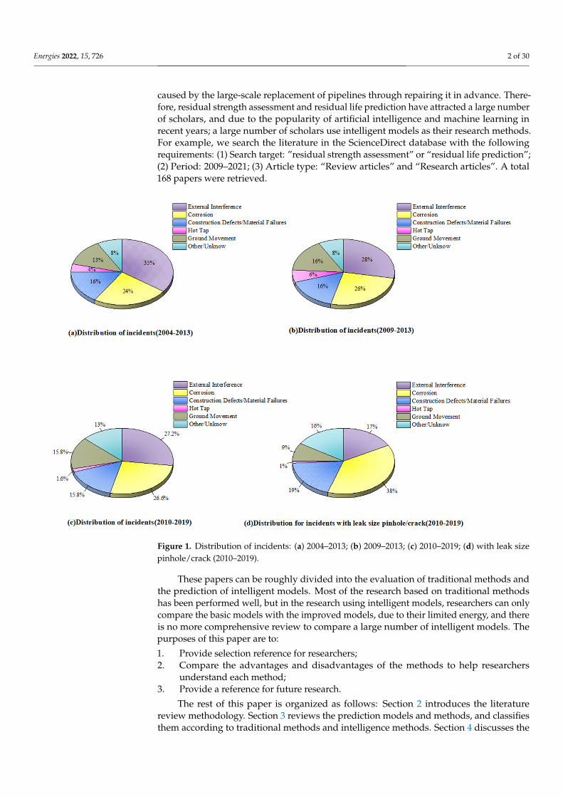
According to the 11th EGIG report [1], incidents caused by corrosion accounted for26% during the period 2009–2013 and 24% during the period 2004–2013, and the incidentscaused by corrosion accounted for 26.63% during the period 2010–2019.The incidents withleak size pinhole/crack caused by corrosion accounted for 38% (Figure 1).

With the frequent accidents caused by corroded pipelines, it is still necessary to domore research on pipeline residual strength evaluation and residual life prediction. Thesignificance of residual strength evaluation and residual life prediction has two aspects:(a) accurate assessment and prediction makes it possible to prevent unnecessary accidentsand casualties; (b) accurate assessment and prediction can avoid the waste of resources

Energies 2022, 15, 726. https://doi.org/10.3390/en15030726 https://www.mdpi.com/journal/energies

https://doi.org/10.3390/en15030726

https://creativecommons.org/

https://creativecommons.org/licenses/by/4.0/

https://creativecommons.org/licenses/by/4.0/

https://www.mdpi.com/journal/energies

https://www.mdpi.com

https://orcid.org/0000-0002-8204-1468

https://doi.org/10.3390/en15030726

https://www.mdpi.com/journal/energies

https://www.mdpi.com/article/10.3390/en15030726?type=check_update&version=1

Energies 2022, 15, 726 2 of 30

caused by the large-scale replacement of pipelines through repairing it in advance. There-fore, residual strength assessment and residual life prediction have attracted a large numberof scholars, and due to the popularity of artificial intelligence and machine learning inrecent years; a large number of scholars use intelligent models as their research methods.For example, we search the literature in the ScienceDirect database with the followingrequirements: (1) Search target: ”residual strength assessment” or “residual life prediction”;(2) Period: 2009–2021; (3) Article type: “Review articles” and “Research articles”. A total168 papers were retrieved.

Energies 2022, 14, x FOR PEER REVIEW 2 of 32

Figure 1. Distribution of incidents: (a) 2004–2013; (b) 2009–2013; (c) 2010–2019; (d) with leak size pinhole/crack (2010–2019).

With the frequent accidents caused by corroded pipelines, it is still necessary to do more research on pipeline residual strength evaluation and residual life prediction. The significance of residual strength evaluation and residual life prediction has two aspects: (a) accurate assessment and prediction makes it possible to prevent unnecessary accidents and casualties; (b) accurate assessment and prediction can avoid the waste of resources caused by the large-scale replacement of pipelines through repairing it in advance. Therefore, residual strength assessment and residual life prediction have attracted a large number of scholars, and due to the popularity of artificial intelligence and machine learning in recent years; a large number of scholars use intelligent models as their research methods. For example, we search the literature in the ScienceDirect database with the following requirements: (1) Search target: ”residual strength assessment” or “residual life prediction”; (2) Period: 2009–2021; (3) Article type: “Review articles” and “Research articles”. A total 168 papers were retrieved.

These papers can be roughly divided into the evaluation of traditional methods and the prediction of intelligent models. Most of the research based on traditional methods has been performed well, but in the research using intelligent models, researchers can only compare the basic models with the improved models, due to their limited energy, and there is no more comprehensive review to compare a large number of intelligent models. The purposes of this paper are to: 1. Provide selection reference for researchers; 2. Compare the advantages and disadvantages of the methods to help researchers

understand each method;

Figure 1. Distribution of incidents: (a) 2004–2013; (b) 2009–2013; (c) 2010–2019; (d) with leak sizepinhole/crack (2010–2019).

These papers can be roughly divided into the evaluation of traditional methods andthe prediction of intelligent models. Most of the research based on traditional methodshas been performed well, but in the research using intelligent models, researchers can onlycompare the basic models with the improved models, due to their limited energy, and thereis no more comprehensive review to compare a large number of intelligent models. Thepurposes of this paper are to:

1. Provide selection reference for researchers;2. Compare the advantages and disadvantages of the methods to help researchers

understand each method;3. Provide a reference for future research.

The rest of this paper is organized as follows: Section 2 introduces the literaturereview methodology. Section 3 reviews the prediction models and methods, and classifiesthem according to traditional methods and intelligence methods. Section 4 discusses the

Energies 2022, 15, 726 3 of 30

applicable conditions of traditional methods, compares the prediction accuracy underdifferent pipe steel grades, and reviews the model, data size, input variable, output value,publishing time, performance of intelligent methods, and the future research directions.Section 5 summarizes the primary conclusions of this paper.

2. Methodology

The methodology of this review is summarized as follows, mainly including four steps:

• Step 1: Multiple database searches.

According to our preliminary search results, there is not enough quantity in a singledatabase. In order to summarize more comprehensively and have more reference value,we have combined the search results of multiple databases. The critical information of thesearch is as follows:

Object: residual life/strength prediction of corroded pipeline.Database: Google Scholar, Web of Science, ASCE, SPE, ScienceDirect, CNKI.Keywords: residual strength, residual life, evaluation method, intelligent model.Language: English.Period: 2009–2021

• Step 2: Review and screening.

In the collected literature, many are related to the residual strength evaluation andresidual life prediction, but the experimental object is not the corroded pipeline. In order toachieve better results and determine that the content is directly related to the residual lifeprediction and residual strength evaluation of the corroded pipeline, we read each papercarefully.

• Step 3: Extracting information from papers.

Read the paper in-depth and extract meaningful information, such as the utilizedmodel, prediction accuracy, data size, proportion of test data set, input variables, andoutput value.

• Step 4: Discussion and conclusion.

Discuss the information extracted in step 3, make a comprehensive review, summarizethe existing research, and put forward possible research directions in the future.

3. Literature Review3.1. Traditional Evaluation Methods3.1.1. ASME B31G-1984

In the late 1960s, Texas Eastern transportation company and American Natural GasAssociation (AGA) conducted relevant research on corroded pipelines and proposed NG-18formula [2]. All subsequent formulas of this series evolved from it, and the expression isshown in Equation (1).

Pf = σf low

(1− A

A0

1− AA0

1M

)(1)

In 1984, ASME B31G-1984, as the earliest residual strength evaluation criterion ofcorroded pipelines [3], was proposed by American Society of Mechanical Engineers basedon NG-18. The specific parameters in NG-18 formula were given. l2

Dt ≤ 20 is defined as ashort defect and l2

Dt ≥ 20 is defined as a long defect. According to different defect length,there are two formulas for calculating failure pressure of pipeline (Equation (2)).

Pf = σf low

(1− A

A0

1− AA0

1M

)(2)

Energies 2022, 15, 726 4 of 30

3.1.2. ASME B31G-1991

In 1991, American Society of Mechanical Engineers had made some modifications toB31G-1984, and proposed ASME B31G-1991 [4]. The new criterion retained the originalflow stress, and modified the Folias bulging coefficient and the calculation formula of longdefect failure pressure, the expression is shown in Equation (3).

Pf =σf low2t

D

(1− d

t

)(3)

Compare to B31G-1984, the results of B31G-1991 evaluation criterion is less conservative.

3.1.3. Modified B31G

Kiefner and others of the American Natural Gas Association (AGA) [5] found thatimproper definition of flow stress, inaccurate expression of the Folias bulging coefficient,and inaccurate calculation of metal loss area caused B31G-1984 to be too conservative.In view of the above problems, Kiefner and his colleagues proposed the modified B31Gcriterion. The modified evaluation criterion does not distinguish the size of defects whensimplifying the projected area of defect profile, but takes A = 0.85 dL. Therefore, thisevaluation method is also called “RSTRENG 0.85 dL evaluation method”. The expressionof failure pressure is shown in Equation (4).

Pf =σf low2t

D

(1− 0.85 d

t

1− 0.85 dt

1M

)(4)

3.1.4. ASME B31G-2009

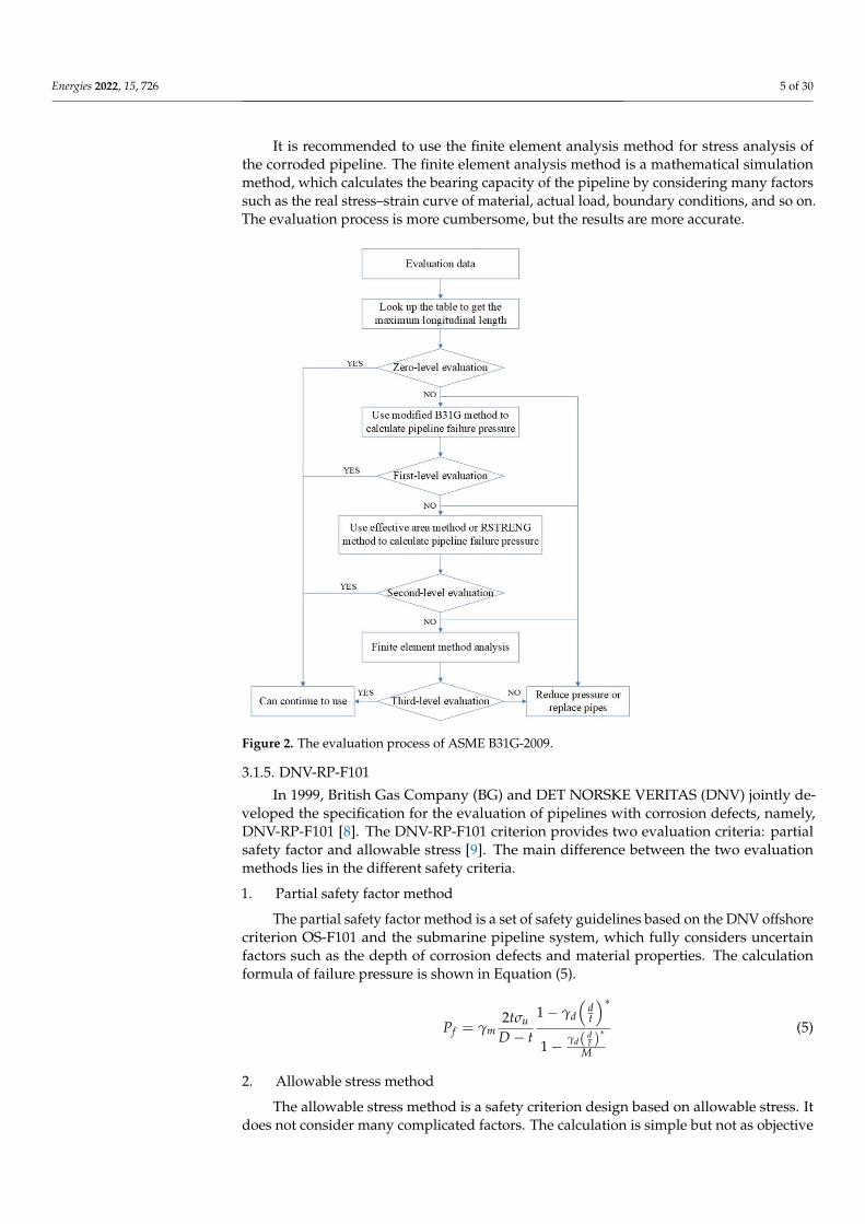
Based on the previous two editions of ASME B31G, the criterion was revised again in2009 and ASME B31G-2009 was obtained [6]. This version adopts the concept of hierarchicalevaluation for the first time (Figure 2). The higher the evaluation level, the more accuratethe evaluation result. However, the difficulty of evaluation also increases [7]. Therefore,different levels of the evaluation methods should be selected according to the actualsituation in the application.

1. Zero-level evaluation

According to the collected corrosion defect parameters and pipeline parameters, querythe table to obtain the maximum allowable length of this defect. If the actual corrosionlength is less than the maximum longitudinal length, it is safe; otherwise, it fails to pass theevaluation. At this time, maintenance measures shall be taken, or a higher-level evaluationmethod shall be selected. The zero-level evaluation is simple to use, but the results areconservative.

2. First-level evaluation

First, calculate the failure pressure of the corroded pipeline by the Modified B31Gmethod, and then compare it with the product of the pipeline safety factor and the operatingpressure for evaluation. The first-level evaluation needs to be completed by professionalssuch as corrosion technicians or coating inspectors.

3. Second-level evaluation

The criterion recommends that the second-level evaluation use the RSTRENG effectivearea method to evaluate the residual strength of corroded pipelines. The effective areamethod has a wide range of applications, and it is also applicable to independent defectsand interacting defect groups. However, it also has certain limitations. The effective areacalculation requires a detailed measurement of the defect size, and software is also required,so it is rarely used in actual working conditions.

4. Third-level evaluation

Energies 2022, 15, 726 5 of 30

It is recommended to use the finite element analysis method for stress analysis ofthe corroded pipeline. The finite element analysis method is a mathematical simulationmethod, which calculates the bearing capacity of the pipeline by considering many factorssuch as the real stress–strain curve of material, actual load, boundary conditions, and so on.The evaluation process is more cumbersome, but the results are more accurate.


The criterion recommends that the second-level evaluation use the RSTRENG effective area method to evaluate the residual strength of corroded pipelines. The effective area method has a wide range of applications, and it is also applicable to independent defects and interacting defect groups. However, it also has certain limitations. The effective area calculation requires a detailed measurement of the defect size, and software is also required, so it is rarely used in actual working conditions. 4. Third-level evaluation

It is recommended to use the finite element analysis method for stress analysis of the corroded pipeline. The finite element analysis method is a mathematical simulation method, which calculates the bearing capacity of the pipeline by considering many factors such as the real stress–strain curve of material, actual load, boundary conditions, and so on. The evaluation process is more cumbersome, but the results are more accurate.

Figure 2. The evaluation process of ASME B31G-2009.

3.1.5. DNV-RP-F101 In 1999, British Gas Company (BG) and DET NORSKE VERITAS (DNV) jointly

developed the specification for the evaluation of pipelines with corrosion defects, namely, DNV-RP-F101 [8]. The DNV-RP-F101 criterion provides two evaluation criteria: partial safety factor and allowable stress [9]. The main difference between the two evaluation methods lies in the different safety criteria. 1. Partial safety factor method

The partial safety factor method is a set of safety guidelines based on the DNV offshore criterion OS-F101 and the submarine pipeline system, which fully considers uncertain factors such as the depth of corrosion defects and material properties. The calculation formula of failure pressure is shown in Equation (5).

Figure 2. The evaluation process of ASME B31G-2009.

3.1.5. DNV-RP-F101

In 1999, British Gas Company (BG) and DET NORSKE VERITAS (DNV) jointly de-veloped the specification for the evaluation of pipelines with corrosion defects, namely,DNV-RP-F101 [8]. The DNV-RP-F101 criterion provides two evaluation criteria: partialsafety factor and allowable stress [9]. The main difference between the two evaluationmethods lies in the different safety criteria.

1. Partial safety factor method

The partial safety factor method is a set of safety guidelines based on the DNV offshorecriterion OS-F101 and the submarine pipeline system, which fully considers uncertainfactors such as the depth of corrosion defects and material properties. The calculationformula of failure pressure is shown in Equation (5).

Pf = γm2tσu

D− t

1− γd

(dt

)∗1− γd( d

t )∗

M

(5)

2. Allowable stress method

The allowable stress method is a safety criterion design based on allowable stress. Itdoes not consider many complicated factors. The calculation is simple but not as objective

Energies 2022, 15, 726 6 of 30

and accurate as the partial safety factor method. The calculation formula of failure pressureis shown in Equation (6).

Pf =σu2t

D− t

(1− d

t

1− dt

1M

)(6)

3.1.6. PCORRC

PCORRC (Pipeline Corrosion Criterion) [10] is a recent evaluation method mainlyused to evaluate the residual strength of the medium and high strength steel pipes withblunt corrosion defects due to plastic instability. This method is obtained by Stephensusing shell elements to simulate corrosion defects. In this method, the failure pressure ofpipelines is determined by tensile strength, not yield strength or flow stress. The calculationformula of failure pressure is shown in Equation (7).

Pf =σu2t

D− t

1− dt

1− exp

−0.157l√Dt−Dd

2

(7)

The failure pressure calculation formula is obtained by fitting the finite elementcalculation results, mainly considering defects’ length and depth.

3.1.7. RSTRENG

On the basis of ASME B31G-1991, Kiefner and Vieth developed the RSTRENG calcula-tion program, called RSTRENG [11] method, by redefining the Folias factor and materialflow stress, and describing the shape of corrosion defects in more detail. RSTRENG ismainly used to evaluate the residual strength of externally corroded pipelines, includingRSTRENG 0.85-area method and RSTRENG effective area method [12].

1. RSTRENG 0.85-area method

RSTRENG only requires two parameters: defect depth and length, but adds the flowstress value defined in ASME B31G. In contrast, ASME B31G is more conservative thanRSTRENG 0.85-area method, and is the same as the modified B31G in the definitions offlow stress, Folias factor, and defect projection area. The calculation formula is shown inEquation (8).

Pf =σf low2t

D

(1− 0.85 d

t

1− 0.85 dt

1M

)(8)

2. RSTRENG effective area method

The RSTRENG effective area evaluation method requires defect depth, defect length,data along the axial and circumferential directions of defects, and detailed corrosion profile.The calculation of the effective area is closer to the actual results. The effective area methodhas higher accuracy, but the calculation is more complex. The calculation formula is shownin Equation (9).

Pf =σf low2t

D

(1− A

A0

1− AA0

1M

)(9)

3.1.8. Others

In addition to the above evaluation methods, there are still some other evaluationmethods, such as SY/T 6151-2009 [13] and BS 7910-2005 [14]. SY/T 6151-2009 “evaluationmethod for corrosion damage of steel pipeline” is the latest oil and gas industry criterion ofChina issued in December 2009.Compared with ASME B31G criterion, SY/T 6151 criterionconsiders the influence of circumferential corrosion length, applies fracture mechanicstheory to determine the maximum safe working pressure, and classifies and evaluatesaccording to the degree of pipeline corrosion damage. The BS7910-2005 method divides

Energies 2022, 15, 726 7 of 30

corrosion defects into single defects and combined defects, and uses tensile strength insteadof flow stress in the calculation formula.

3.1.9. Comparison

Several existing main residual strength evaluation criteria for corroded pipelinesare introduced above, including ASME B31G, modified B31G, DNV-RP-F101, RSTRENG,etc. The above methods have different formula definitions, bulging coefficient and defectarea, and their application scope, applicable defect type, and load type are different. Thecomparison of main criteria and methods is shown in Tables 1 and 2.

Table 1. Comparison of parameters in residual strength evaluation methods.

EvaluationMethod

FlowStress Folias Bulging Coefficient Corrosion Projection

Area

ASME B31G 1.1SMYS M =√

1 + 0.8L2

Dt

23 dl (parabolic);dl (rectangle).

Modified B31G SMYS +68.95 M =

√

1 + 0.6275(

l√Dt

)2− 0.003375

(l

Dt

)4 (l2

Dt ≤ 50)

0.032 l2

Dt + 3.3(

l2

Dt ≥ 50) 0.85dl (between

parabolic and rectangle)

SY/T 6151-2009 SMTS +68.95 M =

√

1 + 0.6275(

l√Dt

)2− 0.003375

(l

Dt

)4 (l2

Dt ≤ 50)

0.032 l2

Dt + 3.3(

l2



DNV-RP-F101 SMTS M =

√1 + 0.31

[L√Dt

]2 dl

PCORRC SMTS — —RSTRENG

0.85-area methodSMTS +

68.95 M =

√

1 + 0.6275(

l√Dt

)2− 0.003375

(l

Dt

)4 (l2

Dt ≤ 50)

0.032 l2

Dt + 3.3(

l2



RSTRENG Effectarea method

SMTS +68.95 M =

√

1 + 0.6275(

l√Dt

)2− 0.003375

(l

Dt

)4 (l2

Dt ≤ 50)

0.032 l2

Dt + 3.3(

l2

Dt ≥ 50) —

Table 2. Comparison of residual strength evaluation methods for pipes with different corrosion defect.

Evaluation Method Best Scope of Application Defect Type Load Type

ASME B31G Medium and low strength steel Isolated defect Internal pressure

Modified B31G Medium and low strength steelIsolated defect or treat the

interaction defect as anisolated defect

Internal pressure

SY/T 6151-2009Carbon steel and low alloy steelpipes with blunt and low stressconcentration corrosion damage

Isolated defect or treat theinteraction defect as an

isolated defectInternal pressure

DNV-RP-F101 Medium and high strength steel Single defect/interactiondefect, complex shape defect

Internal pressure/axialcompressive stress

PCORRC Medium and high strength steelIsolated defect or treat the

interaction defect as anisolated defect

Internal pressure

RSTRENG Effect area Medium and low strength steel Complex shape defect Internal pressure

3.2. Intelligent Methods

In the actual pipeline transportation system, many influencing factors do not havea clear functional relationship, and the practical application effect of traditional methodsis often not ideal. Therefore, some intelligent methods are gradually used in the field ofpipeline corrosion prediction, such as fuzzy mathematics theory method, artificial neuralnetwork method, chaos theory method, support vector machine, and so on.

Energies 2022, 15, 726 8 of 30

3.2.1. ANN

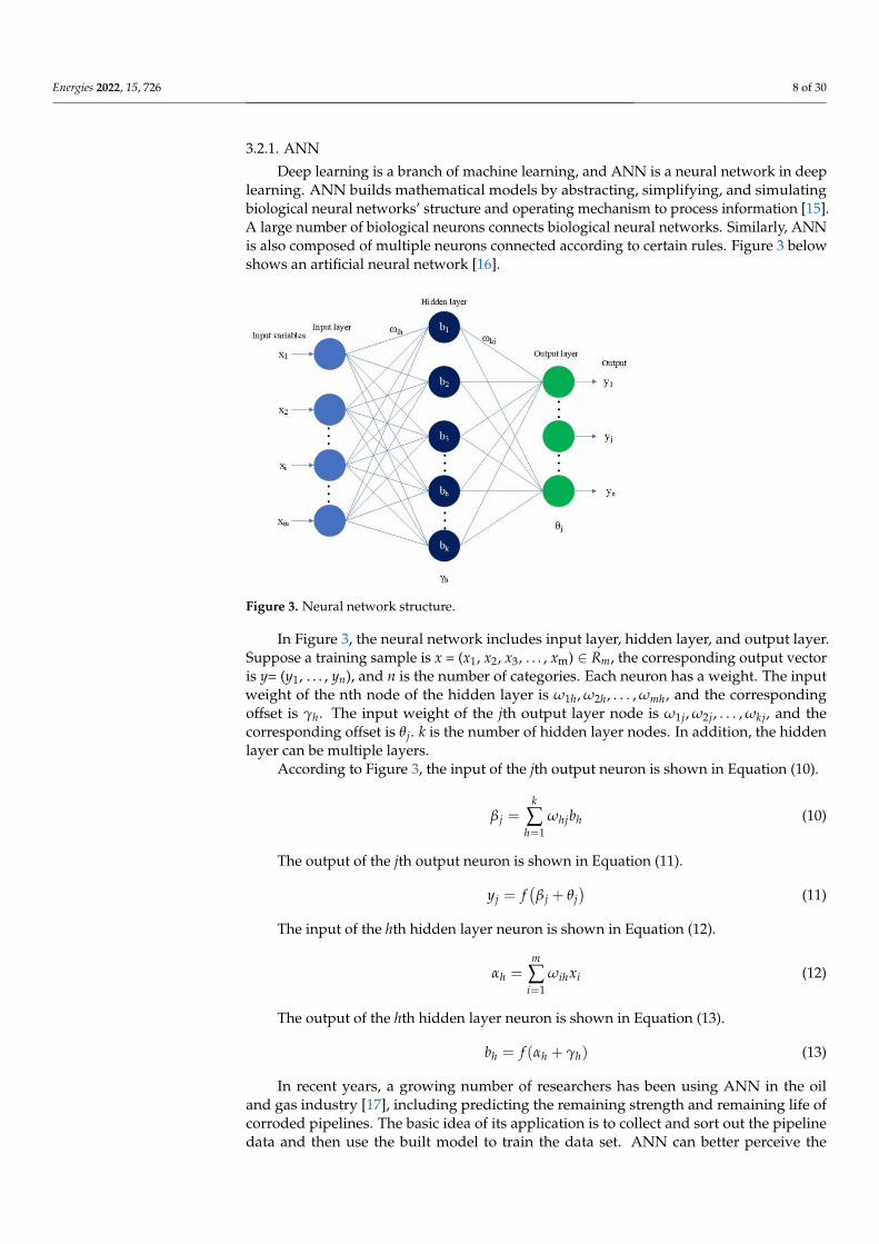
Deep learning is a branch of machine learning, and ANN is a neural network in deeplearning. ANN builds mathematical models by abstracting, simplifying, and simulatingbiological neural networks’ structure and operating mechanism to process information [15].A large number of biological neurons connects biological neural networks. Similarly, ANNis also composed of multiple neurons connected according to certain rules. Figure 3 belowshows an artificial neural network [16].


Figure 3. Neural network structure.

In Figure 3, the neural network includes input layer, hidden layer, and output layer. Suppose a training sample is x = (x1, x2, x3, ..., xm) ∈ Rm, the corresponding output vector is y= (y1, ..., yn), and n is the number of categories. Each neuron has a weight. The input weight of the nth node of the hidden layer is 𝜔 , 𝜔 , . . . , 𝜔 , and the corresponding offset is 𝛾 . The input weight of the jth output layer node is 𝜔 , 𝜔 , . . . , 𝜔 , and the corresponding offset is 𝜃 . k is the number of hidden layer nodes. In addition, the hidden layer can be multiple layers.

According to Figure 3., the input of the jth output neuron is shown in Equation (10).

𝛽 = 𝜔 𝑏 (10)

The output of the jth output neuron is shown in Equation (11). 𝑦 = 𝑓(𝛽 + 𝜃 ) (11)

The input of the hth hidden layer neuron is shown in Equation (12).

𝛼 = 𝜔 𝑥 (12)

The output of the hth hidden layer neuron is shown in Equation (13). 𝑏 = 𝑓(𝛼 + 𝛾 ) (13)

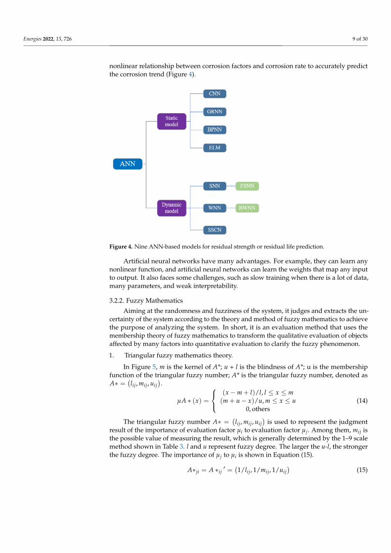
In recent years, a growing number of researchers has been using ANN in the oil and gas industry [17], including predicting the remaining strength and remaining life of corroded pipelines. The basic idea of its application is to collect and sort out the pipeline data and then use the built model to train the data set. ANN can better perceive the nonlinear relationship between corrosion factors and corrosion rate to accurately predict the corrosion trend (Figure 4).

Artificial neural networks have many advantages. For example, they can learn any nonlinear function, and artificial neural networks can learn the weights that map any input to output. It also faces some challenges, such as slow training when there is a lot of data, many parameters, and weak interpretability.

Figure 3. Neural network structure.

In Figure 3, the neural network includes input layer, hidden layer, and output layer.Suppose a training sample is x = (x1, x2, x3, . . . , xm) ∈ Rm, the corresponding output vectoris y= (y1, . . . , yn), and n is the number of categories. Each neuron has a weight. The inputweight of the nth node of the hidden layer is ω1h, ω2h, . . . , ωmh, and the correspondingoffset is γh. The input weight of the jth output layer node is ω1j, ω2j, . . . , ωkj, and thecorresponding offset is θj. k is the number of hidden layer nodes. In addition, the hiddenlayer can be multiple layers.

According to Figure 3, the input of the jth output neuron is shown in Equation (10).

β j =k

∑h=1

ωhjbh (10)

The output of the jth output neuron is shown in Equation (11).

yj = f(

β j + θj)

(11)

The input of the hth hidden layer neuron is shown in Equation (12).

αh =m

∑i=1

ωihxi (12)

The output of the hth hidden layer neuron is shown in Equation (13).

bh = f (αh + γh) (13)

In recent years, a growing number of researchers has been using ANN in the oiland gas industry [17], including predicting the remaining strength and remaining life ofcorroded pipelines. The basic idea of its application is to collect and sort out the pipelinedata and then use the built model to train the data set. ANN can better perceive the

Energies 2022, 15, 726 9 of 30

nonlinear relationship between corrosion factors and corrosion rate to accurately predictthe corrosion trend (Figure 4).


Figure 4. Nine ANN-based models for residual strength or residual life prediction.

3.2.2. Fuzzy Mathematics Aiming at the randomness and fuzziness of the system, it judges and extracts the

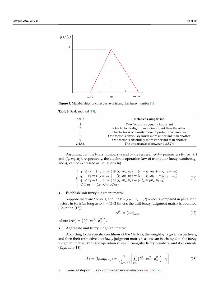
uncertainty of the system according to the theory and method of fuzzy mathematics to achieve the purpose of analyzing the system. In short, it is an evaluation method that uses the membership theory of fuzzy mathematics to transform the qualitative evaluation of objects affected by many factors into quantitative evaluation to clarify the fuzzy phenomenon. 1. Triangular fuzzy mathematics theory.

In Figure 5, m is the kernel of A*; u + l is the blindness of A*; u is the membership function of the triangular fuzzy number; A* is the triangular fuzzy number, denoted as 𝐴 ∗= 𝑙 , 𝑚 , 𝑢 .

𝜇𝐴 ∗ (𝑥) = (𝑥 − 𝑚 + 𝑙)/𝑙, 𝑙 ≤ 𝑥 ≤ 𝑚(𝑚 + 𝑢 − 𝑥)/𝑢, 𝑚 ≤ 𝑥 ≤ 𝑢0, 𝑜𝑡ℎ𝑒𝑟𝑠 (14)

The triangular fuzzy number 𝐴 ∗= 𝑙 , 𝑚 , 𝑢 is used to represent the judgment result of the importance of evaluation factor 𝜇 to evaluation factor 𝜇 . Among them, 𝑚 is the possible value of measuring the result, which is generally determined by the 1-9 scale method shown in Table 3. l and u represent fuzzy degree. The larger the u-l, the stronger the fuzzy degree. The importance of 𝜇 to 𝜇 is shown in Equation (15). 𝐴 ∗ = 𝐴 ∗ = (1/𝑙 , 1/𝑚 , 1/𝑢 ) (15)

Assuming that the fuzzy numbers q1 and q2 are represented by parameters (l1, m1, u1) and (l2, m2, u2), respectively, the algebraic operation law of triangular fuzzy numbers q1 and q2 can be expressed as Equation (16).

( ) ( ) ( )( ) ( ) ( )( ) ( ) ( )( )

1 2 1 1 1 2 2 2 1 2 1 2 1 2

1 2 1 1 1 2 2 2 1 2 1 2 1 2

1 2 1 1 1 2 2 2 1 2 1 2 1 2

1 1 1 1

, , , , , ,, , , , , ,

, , , , , ,, ,

q q l m u l m u l l m m u u



C q Cl Cm Cu

⊕ = ⊕ = + + +

− = − = − − −

⊗ = ⊗ = ⊗ ⊗ ⊗ ⊗ =

(16)

Figure 4. Nine ANN-based models for residual strength or residual life prediction.

Artificial neural networks have many advantages. For example, they can learn anynonlinear function, and artificial neural networks can learn the weights that map any inputto output. It also faces some challenges, such as slow training when there is a lot of data,many parameters, and weak interpretability.

3.2.2. Fuzzy Mathematics

Aiming at the randomness and fuzziness of the system, it judges and extracts the un-certainty of the system according to the theory and method of fuzzy mathematics to achievethe purpose of analyzing the system. In short, it is an evaluation method that uses themembership theory of fuzzy mathematics to transform the qualitative evaluation of objectsaffected by many factors into quantitative evaluation to clarify the fuzzy phenomenon.

1. Triangular fuzzy mathematics theory.

In Figure 5, m is the kernel of A*; u + l is the blindness of A*; u is the membershipfunction of the triangular fuzzy number; A* is the triangular fuzzy number, denoted asA∗ =

(lij, mij, uij

).

µA ∗ (x) =

(x−m + l)/l, l ≤ x ≤ m(m + u− x)/u, m ≤ x ≤ u

0, others(14)

The triangular fuzzy number A∗ =(lij, mij, uij

)is used to represent the judgment

result of the importance of evaluation factor µi to evaluation factor µj. Among them, mij isthe possible value of measuring the result, which is generally determined by the 1–9 scalemethod shown in Table 3. l and u represent fuzzy degree. The larger the u-l, the strongerthe fuzzy degree. The importance of µj to µi is shown in Equation (15).

A∗ji = A ∗ij′ =

(1/lij, 1/mij, 1/uij

)(15)

Energies 2022, 15, 726 10 of 30Energies 2022, 14, x FOR PEER REVIEW 11 of 32

Figure 5. Membership function curve of triangular fuzzy number [18].

Table 3. Scale method[19].

Scale Relative Comparison 1 Two factors are equally important 3 One factor is slightly more important than the other 5 One factor is obviously more important than another 7 One factor is obviously much more important than another 9 One factor is absolutely more important than another

2,4,6,8 The importance is between 1.3.5.7.9

• Establish unit fuzzy judgment matrix. Suppose there are t objects, and the kth (k=1, 2, ..., t) object is compared in pairs for n

factors in turn (as long as n(n − 1)/2 times), the unit fuzzy judgment matrix is obtained (Equation (17)). 𝐴( ) = (𝐴 ∗) (17)

where (𝐴 ∗) = 𝑙( ), 𝑚( ), 𝑢( ) .

• Aggregate unit fuzzy judgment matrix. According to the specific conditions of the t factors, the weight 𝑟 is given

respectively, and then their respective unit fuzzy judgment matrix seasons can be changed to the fuzzy judgment matrix A* by the operation rules of triangular fuzzy numbers, and its elements (Equation (18))

𝐴 ∗= (𝑙 , 𝑚 , 𝑢 ) = 1∑ 𝑟 𝑙( ), 𝑚( ), 𝑢( ) ⋅ 𝑟 (18)

2. General steps of fuzzy comprehensive evaluation method [20]. • Establish factor set 𝑋 = (𝑋 , 𝑋 , . . . , 𝑋 ) ,which is composed of evaluation indexes;

Construct weight vector 𝐴 = (𝑎 , 𝑎 , . . . , 𝑎 ). Define the comment set as 𝑊 =(𝑤 , 𝑤 , . . . , 𝑤 ) , and obtain the corresponding weight set Y of the factor set 𝑌 =(𝑌 , 𝑌 , . . . , 𝑌 ). • Construct weight vector 𝐴 = (𝑎 , 𝑎 , . . . , 𝑎 ). • Construct evaluation matrix (Equation (19)).

Figure 5. Membership function curve of triangular fuzzy number [18].

Table 3. Scale method [19].

Scale Relative Comparison

1 Two factors are equally important3 One factor is slightly more important than the other5 One factor is obviously more important than another7 One factor is obviously much more important than another9 One factor is absolutely more important than another

2,4,6,8 The importance is between 1.3.5.7.9

Assuming that the fuzzy numbers q1 and q2 are represented by parameters (l1, m1, u1)and (l2, m2, u2), respectively, the algebraic operation law of triangular fuzzy numbers q1and q2 can be expressed as Equation (16).

q1 ⊕ q2 = (l1, m1, u1)⊕ (l2, m2, u2) = (l1 + l2, m1 + m2, u1 + u2)q1 − q2 = (l1, m1, u1)− (l2, m2, u2) = (l1 − l2, m1 −m2, u1 − u2)q1 ⊗ q2 = (l1, m1, u1)⊗ (l2, m2, u2) = (l1l2, m1m2, u1u2)C⊗ q1 = (Cl1, Cm1, Cu1)

(16)

• Establish unit fuzzy judgment matrix.

Suppose there are t objects, and the kth (k = 1, 2, . . . , t) object is compared in pairs for nfactors in turn (as long as n(n − 1)/2 times), the unit fuzzy judgment matrix is obtained(Equation (17)).

A(k) = (A∗)n×n (17)

where (A∗) =(

l(k)ij , m(k)ij , u(k)

ij

).

• Aggregate unit fuzzy judgment matrix.

According to the specific conditions of the t factors, the weight rk is given respectively,and then their respective unit fuzzy judgment matrix seasons can be changed to the fuzzyjudgment matrix A* by the operation rules of triangular fuzzy numbers, and its elements(Equation (18))

A∗ =(lij, mij, uij

)=

1

∑tK=1 rk

[t

∑k=1

(l(k)ij , m(k)

ij , u(k)ij

)· rk

](18)

2. General steps of fuzzy comprehensive evaluation method [20].

Energies 2022, 15, 726 11 of 30

• Establish factor set X = (X1, X2, . . . , Xi), which is composed of evaluation indexes;Construct weight vector A = (a1, a2, . . . , ai). Define the comment set as W = (w1, w2,. . . , wi), and obtain the corresponding weight set Y of the factor set Y = (Y1, Y2, . . . , Yi).

• Construct weight vector A = (a1, a2, . . . , ai).

• Construct evaluation matrix (Equation (19)).

R =

r11 r12 . . . r1jr21 r22 . . . r2j. . . . . . . . . . . .ri1 ri2 . . . rij

(19)

where rxy(x = 1, 2, . . . , i; y = 1, 2, . . . , j) represents the degree of membership of thefactor level index Xx to the yth comment set wy.

• Calculate fuzzy matrix.

Obtain the membership vector B of the factor layer index to the comment set(Equation (20)):

B = YR = (Y1, Y2, . . . , Yi)

r11 r12 . . . r1jr21 r22 . . . r2j. . . . . . . . . . . .ri1 ri2 . . . rij

=(b1, b2, . . . , bj

)(20)

when ∑jx=1 bx 6= 1, let b∗x = bx/ ∑

jx=1 bx to obtain (Equation (21)):

B∗ =(

b∗1 , b∗2 , . . . , b∗j)

(21)

where B* is the membership vector of target layer index x to comment set W. According tothe specific content of B*, the corresponding evaluation can be obtained.

3.2.3. Chaos Theory and Method

In 1905, H. Poincare discovered chaos for the first time in his research and put forwardthe H. Poincare conjecture: a small error in the initial conditions produces a great errorin the final phenomenon, so the prediction becomes impossible. In 1963, the Americanmeteorologist Lorenz discovered in numerical experiments that deterministic systemssometimes exhibit random behavior phenomena, and then he called it “deterministicnonperiodic flow” in the literature [21]. In 1975, Li TY and Yorke gave a specific definitionof chaos for the first time [22]: chaos is a kind of random and random phenomenon thatoccurs in a deterministic system and is sensitive to initial conditions. It is a phenomenonthat exists widely in nature.

The mathematics model of Chaos:

• Collect a digital sequence (x0, x1, x2, . . . , xi, . . . , xs) of a certain characteristic quantityof the observed system.

• Using difference can generate new first-order difference sequence, second-order differ-ence sequence. . . (Equations (22) and (23)).

∆xn = xn+1 − xn (22)

∆(∆x) = ∆2x (23)

• Take the number of observations as the horizontal axis and the characteristic quantityas the vertical axis to make a graph, which can intuitively and qualitatively grasp thetime structure and trend of the phenomenon change.

• Based on the prediction sequence, calculate any item with one or more items in frontof the sequence by assuming the changing structure (Equation (24)):

Energies 2022, 15, 726 12 of 30

xn+1 = f (xn) = f ( f (xn−1)) = f 2(xn−1) = f n(x0) (24)

Chaos theory is the analysis of irregular and unpredictable phenomena and processes.In essence, a chaotic process is a deterministic process, but it is disorderly, fuzzy, andrandom on the surface. This is similar to the corrosion development process of pipelinesystem, but the required sample size must be sufficient.

3.2.4. SVM

Support vector machine, which Cortes and Vapnik first proposed in 1995 [23], isa practical algorithm for nonlinear classification and regression problems in the case ofsmall samples. When dealing with the regression problem, the basic idea is to map thelow-dimensional nonlinear regression problem to the high-dimensional feature space, andestablish a model in the high-dimensional feature space to learn the data set for regressionfitting [24].

Using the basic idea of support vector machine, the data set (x1, x2, . . . , xn) is mappedto a high-dimensional feature space, and then the data set X is used to establish a model inthis space for linear regression. The regression form is as Equation (25).

f (xi) = ω · ϕ(xi) + b (25)

where ω, b is regression factor, φ is the coefficient to be determined in the model.In order to obtain the regression function, the above problem is transformed into the

following planning problem (Equation (25)).

min12

ωTω + Cn

∑i=1

ξi + Cn

∑i=1

ξi∗ (26)

Constraints are:

s.t.

yi −ω · ϕ(xi)− b ≤ ε + ξ∗iω · ϕ(xi) + b− yi ≤ ε + ξi

ξi, ξ∗i ≥ 0

where C is the penalty term constant, ε is the insensitive loss function, and ζi, ζ∗i are theslack variables.

By introducing Lagrange function, the above optimization problem can be transformedinto Lagrange dual problem, and the solution is as follows:

f (x) =l

∑i=1

(αi − α∗i )K(Xd, X) + b (27)

where ai, a∗i is the Lagrange multiplier, when(ai − a∗i

)is not 0, the corresponding sample

is support vector; K(Xd, X) is the kernel function, the selection of kernel function shouldmake it a point product of high-dimensional feature space.

SVM as a typical machine learning method, is widely used in classification andregression. It can avoid the neural network falling into local optimization, and it is usuallyused in the case of small amount of data such as pipeline corrosion failure.

3.2.5. Comparison

Choosing appropriate methods can effectively improve the evaluation effect andprediction accuracy. The advantages and disadvantages of each method are listed in Table 4to facilitate researchers choosing and using a suitable method.

Energies 2022, 15, 726 13 of 30

Table 4. Merits and limitations of various methods.

Methods Merit Limitation

ANN

It has strong robustness and fault tolerance tonoise neural network, can fully approach complex

nonlinear relations, and has the function ofassociative memory.

Neural network needs a large number ofparameters and its interpretability is not strong.

Fuzzy mathematics

It is able to make a more scientific, reasonable, andrealistic quantitative evaluation of the data with

the hidden information presenting fuzziness. Theevaluation result is a vector, not a point value. Itcontains rich information that can describe the

evaluated object more accurately and be furtherprocessed to obtain reference information.

The calculation is complicated, and thedetermination of the index weight vector issubjective. When the index set is large, it is

difficult to compare the membership degrees, andeven causes the evaluation to fail.

Chaos theoryIt can effectively explain or solve nonlinear

complex problems, and has obvious effect inshort-term prediction.

Chaos behavior is very sensitive to initialconditions, so sufficient and accurate data are

required. The effect of long-term prediction is poor.

SVMIt can achieve good performance under less data,

and has good generalization performance, which isnot easy to over fit.

The speed of large-scale training samples is slow.The traditional SVM is not suitable for multiclassification and is sensitive to missing data,

parameters, and kernel function.

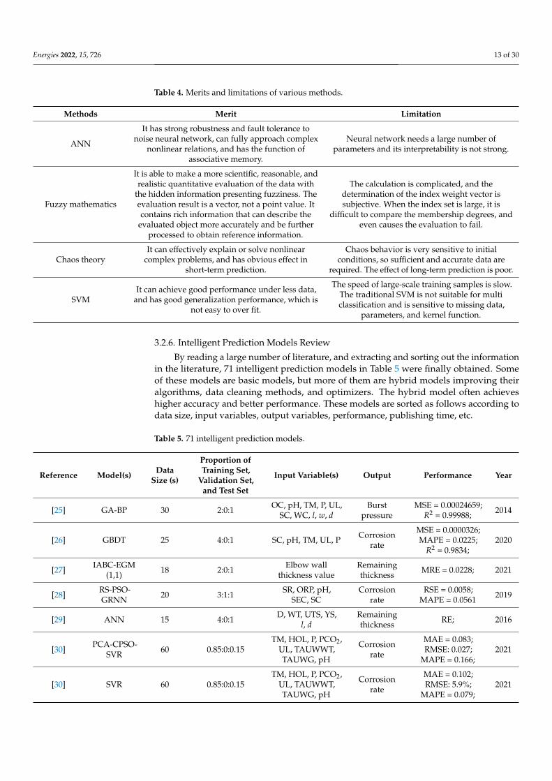
3.2.6. Intelligent Prediction Models Review

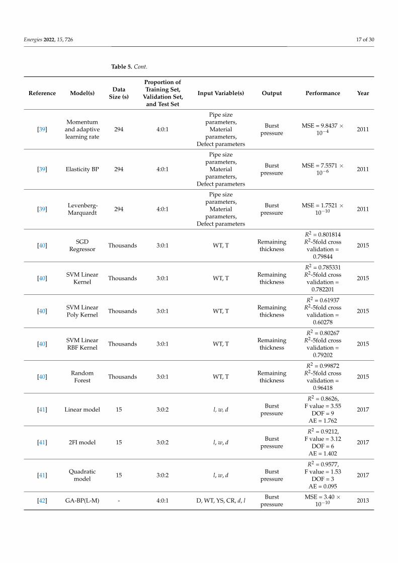
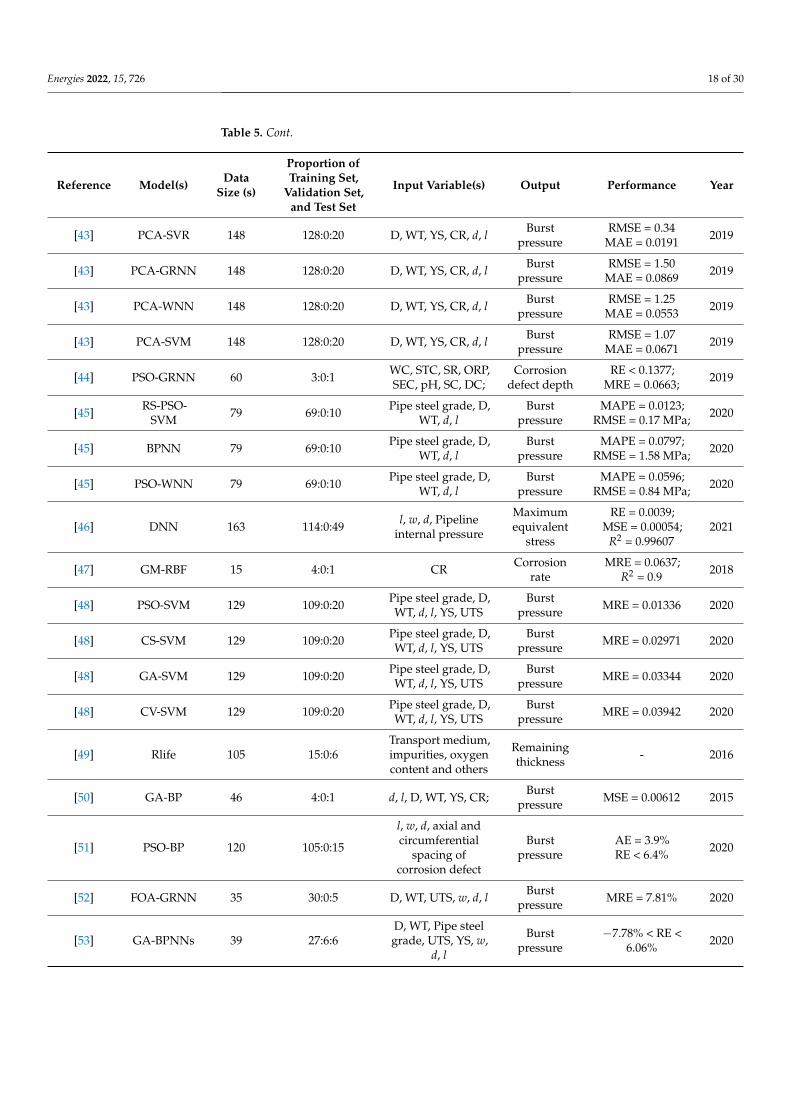
By reading a large number of literature, and extracting and sorting out the informationin the literature, 71 intelligent prediction models in Table 5 were finally obtained. Someof these models are basic models, but more of them are hybrid models improving theiralgorithms, data cleaning methods, and optimizers. The hybrid model often achieveshigher accuracy and better performance. These models are sorted as follows according todata size, input variables, output variables, performance, publishing time, etc.

Table 5. 71 intelligent prediction models.

Reference Model(s) DataSize (s)

Proportion ofTraining Set,

Validation Set,and Test Set

Input Variable(s) Output Performance Year

[25] GA-BP 30 2:0:1 OC, pH, TM, P, UL,SC, WC, l, w, d

Burstpressure

MSE = 0.00024659;R2 = 0.99988; 2014

[26] GBDT 25 4:0:1 SC, pH, TM, UL, P Corrosionrate

MSE = 0.0000326;MAPE = 0.0225;

R2 = 0.9834;2020

[27] IABC-EGM(1,1) 18 2:0:1 Elbow wall

thickness valueRemainingthickness MRE = 0.0228; 2021

[28] RS-PSO-GRNN 20 3:1:1 SR, ORP, pH,

SEC, SCCorrosion

rateRSE = 0.0058;

MAPE = 0.0561 2019

[29] ANN 15 4:0:1 D, WT, UTS, YS,l, d

Remainingthickness RE; 2016

[30] PCA-CPSO-SVR 60 0.85:0:0.15

TM, HOL, P, PCO2,UL, TAUWWT,TAUWG, pH

Corrosionrate

MAE = 0.083;RMSE: 0.027;

MAPE = 0.166;2021

[30] SVR 60 0.85:0:0.15TM, HOL, P, PCO2,

UL, TAUWWT,TAUWG, pH

Corrosionrate

MAE = 0.102;RMSE: 5.9%;

MAPE = 0.079;2021

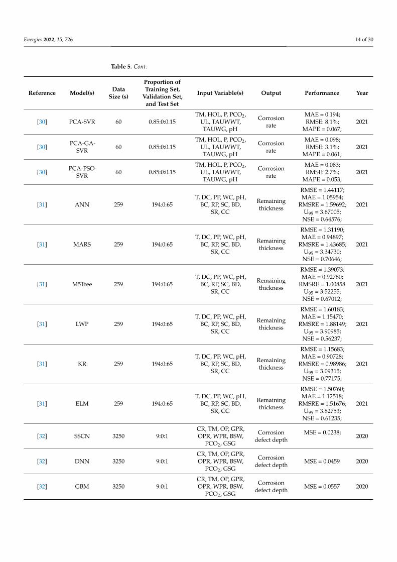
Energies 2022, 15, 726 14 of 30

Table 5. Cont.





[30] PCA-SVR 60 0.85:0:0.15TM, HOL, P, PCO2,

UL, TAUWWT,TAUWG, pH

Corrosionrate

MAE = 0.194;RMSE: 8.1%;

MAPE = 0.067;2021

[30] PCA-GA-SVR 60 0.85:0:0.15


Corrosionrate

MAE = 0.098;RMSE: 3.1%;

MAPE = 0.061;2021

[30] PCA-PSO-SVR 60 0.85:0:0.15


Corrosionrate

MAE = 0.083;RMSE: 2.7%;

MAPE = 0.053;2021

[31] ANN 259 194:0:65T, DC, PP, WC, pH,

BC, RP, SC, BD,SR, CC

Remainingthickness

RMSE = 1.44117;MAE = 1.05954;

RMSRE = 1.59692;U95 = 3.67005;NSE = 0.64576;

2021

[31] MARS 259 194:0:65T, DC, PP, WC, pH,


Remainingthickness

RMSE = 1.31190;MAE = 0.94897;

RMSRE = 1.43685;U95 = 3.34730;NSE = 0.70646;

2021

[31] M5Tree 259 194:0:65T, DC, PP, WC, pH,


Remainingthickness

RMSE = 1.39073;MAE = 0.92780;

RMSRE = 1.00858U95 = 3.52255;NSE = 0.67012;

2021

[31] LWP 259 194:0:65T, DC, PP, WC, pH,


Remainingthickness

RMSE = 1.60183;MAE = 1.15470;

RMSRE = 1.88149;U95 = 3.90985;NSE = 0.56237;

2021

[31] KR 259 194:0:65T, DC, PP, WC, pH,


Remainingthickness

RMSE = 1.15683;MAE = 0.90728;

RMSRE = 0.98986;U95 = 3.09315;NSE = 0.77175;

2021

[31] ELM 259 194:0:65T, DC, PP, WC, pH,


Remainingthickness

RMSE = 1.50760;MAE = 1.12518;

RMSRE = 1.51676;U95 = 3.82753;NSE = 0.61235;

2021

[32] SSCN 3250 9:0:1CR, TM, OP, GPR,OPR, WPR, BSW,

PCO2, GSG

Corrosiondefect depth

MSE = 0.0238; 2020

[32] DNN 3250 9:0:1CR, TM, OP, GPR,OPR, WPR, BSW,

PCO2, GSG

Corrosiondefect depth MSE = 0.0459 2020

[32] GBM 3250 9:0:1CR, TM, OP, GPR,OPR, WPR, BSW,

PCO2, GSG


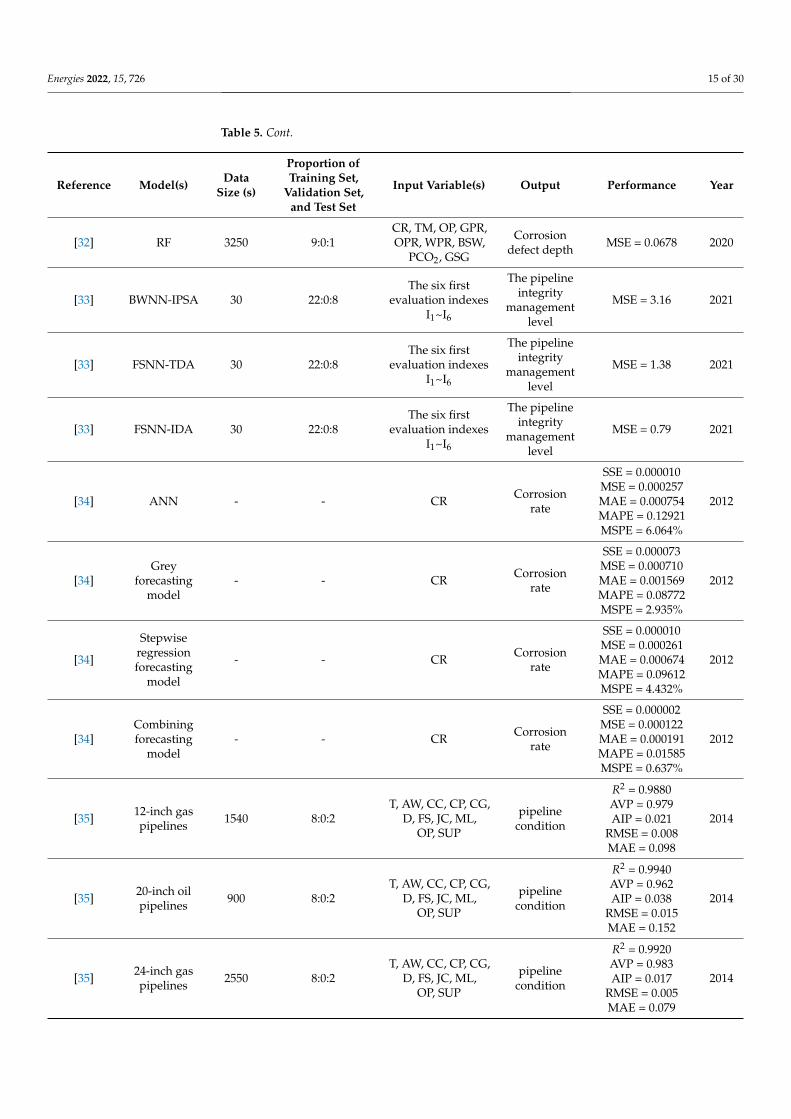
Energies 2022, 15, 726 15 of 30

Table 5. Cont.





[32] RF 3250 9:0:1CR, TM, OP, GPR,OPR, WPR, BSW,

PCO2, GSG


[33] BWNN-IPSA 30 22:0:8The six first

evaluation indexesI1~I6

The pipelineintegrity

managementlevel

MSE = 3.16 2021

[33] FSNN-TDA 30 22:0:8The six first



managementlevel

MSE = 1.38 2021

[33] FSNN-IDA 30 22:0:8The six first



managementlevel

MSE = 0.79 2021

[34] ANN - - CR Corrosionrate

SSE = 0.000010MSE = 0.000257MAE = 0.000754MAPE = 0.12921MSPE = 6.064%

2012

[34]Grey

forecastingmodel

- - CR Corrosionrate


2012

[34]

Stepwiseregressionforecasting

model

- - CR Corrosionrate


2012

[34]Combiningforecasting

model- - CR Corrosion

rate


2012

[35] 12-inch gaspipelines 1540 8:0:2

T, AW, CC, CP, CG,D, FS, JC, ML,

OP, SUP

pipelinecondition

R2 = 0.9880AVP = 0.979AIP = 0.021

RMSE = 0.008MAE = 0.098

2014

[35] 20-inch oilpipelines 900 8:0:2


OP, SUP

pipelinecondition

R2 = 0.9940AVP = 0.962AIP = 0.038

RMSE = 0.015MAE = 0.152

2014

[35] 24-inch gaspipelines 2550 8:0:2


OP, SUP

pipelinecondition

R2 = 0.9920AVP = 0.983AIP = 0.017

RMSE = 0.005MAE = 0.079

2014

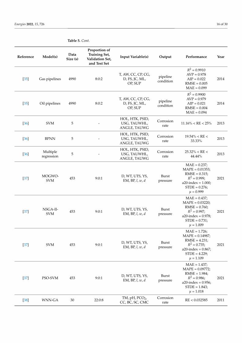
Energies 2022, 15, 726 16 of 30

Table 5. Cont.





[35] Gas pipelines 4990 8:0:2T, AW, CC, CP, CG,

D, FS, JC, ML,OP, SUP

pipelinecondition

R2 = 0.9910AVP = 0.978AIP = 0.022

RMSE = 0.005MAE = 0.099

2014

[35] Oil pipelines 4990 8:0:2T, AW, CC, CP, CG,

D, FS, JC, ML,OP, SUP

pipelinecondition

R2 = 0.9900AVP = 0.979AIP = 0.021

RMSE = 0.004MAE = 0.094

2014

[36] SVM 5 -HOL, HTK, PSID,USG, TAUWHL,

ANGLE, TAUWG

Corrosionrate 11.16% < RE < 25% 2013

[36] BPNN 5 -HOL, HTK, PSID,USG, TAUWHL,

ANGLE, TAUWG

Corrosionrate

19.54% < RE <33.33% 2013

[36] Multipleregression 5 -

HOL, HTK, PSID,USG, TAUWHL,

ANGLE, TAUWG

Corrosionrate

25.32% < RE <44.44% 2013

[37] MOGWO-SVM 453 9:0:1 D, WT, UTS, YS,

EM, BP, l, w, dBurst

pressure

MAE = 0.237;MAPE = 0.01353;

RMSE = 0.315;R2 = 0.999;

a20-index = 1.000;STDE = 0.276;

µ = 0.999

2021

[37] NSGA-II-SVM 453 9:0:1 D, WT, UTS, YS,

EM, BP, l, w, dBurst

pressure

MAE = 0.437;MAPE = 0.03220;

RMSE = 0.760;R2 = 0.997;

a20-index = 0.978;STDE = 0.731;

µ = 1.009

2021

[37] SVM 453 9:0:1 D, WT, UTS, YS,EM, BP, l, w, d

Burstpressure

MAE = 1.726;MAPE = 0.14987;

RMSE = 4.231;R2 = 0.735;

a20-index = 0.867;STDE = 4.229;

µ = 1.109

2021

[37] PSO-SVM 453 9:0:1 D, WT, UTS, YS,EM, BP, l, w, d

Burstpressure

MAE = 1.437;MAPE = 0.09772;

RMSE = 1.984;R2 = 0.986;

a20-index = 0.956;STDE = 1.843;

µ = 1.018

2021

[38] WNN-GA 30 22:0:8 TM, pH, PCO2,CC, BC, SC, CMC

Corrosionrate RE < 0.032585 2011

Energies 2022, 15, 726 17 of 30

Table 5. Cont.





[39]Momentum

and adaptivelearning rate

294 4:0:1

Pipe sizeparameters,

Materialparameters,

Defect parameters

Burstpressure

MSE = 9.8437 ×10−4 2011

[39] Elasticity BP 294 4:0:1


Materialparameters,

Defect parameters

Burstpressure

MSE = 7.5571 ×10−6 2011

[39] Levenberg-Marquardt 294 4:0:1


Materialparameters,

Defect parameters

Burstpressure

MSE = 1.7521 ×10−10 2011

[40] SGDRegressor Thousands 3:0:1 WT, T Remaining

thickness

R2 = 0.801814R2-5fold crossvalidation =

0.79844

2015

[40] SVM LinearKernel Thousands 3:0:1 WT, T Remaining

thickness


0.782201

2015

[40] SVM LinearPoly Kernel Thousands 3:0:1 WT, T Remaining

thickness


0.60278

2015

[40] SVM LinearRBF Kernel Thousands 3:0:1 WT, T Remaining

thickness


0.79202

2015

[40] RandomForest Thousands 3:0:1 WT, T Remaining

thickness


0.96418

2015

[41] Linear model 15 3:0:2 l, w, d Burstpressure

R2 = 0.8626,F value = 3.55

DOF = 9AE = 1.762

2017

[41] 2FI model 15 3:0:2 l, w, d Burstpressure

R2 = 0.9212,F value = 3.12

DOF = 6AE = 1.402

2017

[41] Quadraticmodel 15 3:0:2 l, w, d Burst

pressure

R2 = 0.9577,F value = 1.53

DOF = 3AE = 0.095

2017

[42] GA-BP(L-M) - 4:0:1 D, WT, YS, CR, d, l Burstpressure

MSE = 3.40 ×10−10 2013

Energies 2022, 15, 726 18 of 30

Table 5. Cont.





[43] PCA-SVR 148 128:0:20 D, WT, YS, CR, d, l Burstpressure

RMSE = 0.34MAE = 0.0191 2019

[43] PCA-GRNN 148 128:0:20 D, WT, YS, CR, d, l Burstpressure

RMSE = 1.50MAE = 0.0869 2019

[43] PCA-WNN 148 128:0:20 D, WT, YS, CR, d, l Burstpressure

RMSE = 1.25MAE = 0.0553 2019

[43] PCA-SVM 148 128:0:20 D, WT, YS, CR, d, l Burstpressure

RMSE = 1.07MAE = 0.0671 2019

[44] PSO-GRNN 60 3:0:1 WC, STC, SR, ORP,SEC, pH, SC, DC;

Corrosiondefect depth

RE < 0.1377;MRE = 0.0663; 2019

[45] RS-PSO-SVM 79 69:0:10 Pipe steel grade, D,

WT, d, lBurst

pressureMAPE = 0.0123;

RMSE = 0.17 MPa; 2020

[45] BPNN 79 69:0:10 Pipe steel grade, D,WT, d, l

Burstpressure

MAPE = 0.0797;RMSE = 1.58 MPa; 2020

[45] PSO-WNN 79 69:0:10 Pipe steel grade, D,WT, d, l

Burstpressure

MAPE = 0.0596;RMSE = 0.84 MPa; 2020

[46] DNN 163 114:0:49 l, w, d, Pipelineinternal pressure

Maximumequivalent

stress

RE = 0.0039;MSE = 0.00054;

R2 = 0.996072021

[47] GM-RBF 15 4:0:1 CR Corrosionrate

MRE = 0.0637;R2 = 0.9 2018

[48] PSO-SVM 129 109:0:20 Pipe steel grade, D,WT, d, l, YS, UTS

Burstpressure MRE = 0.01336 2020

[48] CS-SVM 129 109:0:20 Pipe steel grade, D,WT, d, l, YS, UTS


[48] GA-SVM 129 109:0:20 Pipe steel grade, D,WT, d, l, YS, UTS


[48] CV-SVM 129 109:0:20 Pipe steel grade, D,WT, d, l, YS, UTS


[49] Rlife 105 15:0:6Transport medium,impurities, oxygencontent and others

Remainingthickness - 2016

[50] GA-BP 46 4:0:1 d, l, D, WT, YS, CR; Burstpressure MSE = 0.00612 2015

[51] PSO-BP 120 105:0:15

l, w, d, axial andcircumferential

spacing ofcorrosion defect

Burstpressure

AE = 3.9%RE < 6.4% 2020

[52] FOA-GRNN 35 30:0:5 D, WT, UTS, w, d, l Burstpressure MRE = 7.81% 2020

[53] GA-BPNNs 39 27:6:6D, WT, Pipe steelgrade, UTS, YS, w,

d, l

Burstpressure

−7.78% < RE <6.06% 2020

Energies 2022, 15, 726 19 of 30

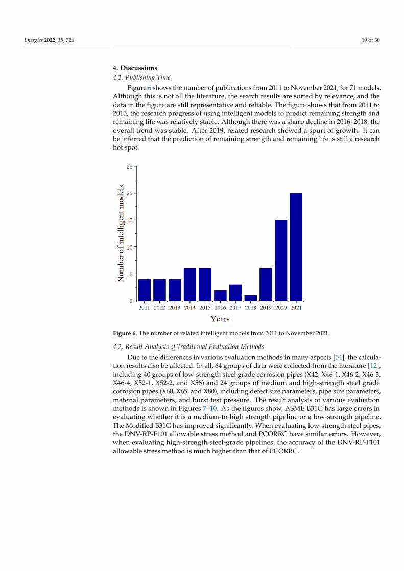
4. Discussions4.1. Publishing Time

Figure 6 shows the number of publications from 2011 to November 2021, for 71 models.Although this is not all the literature, the search results are sorted by relevance, and thedata in the figure are still representative and reliable. The figure shows that from 2011 to2015, the research progress of using intelligent models to predict remaining strength andremaining life was relatively stable. Although there was a sharp decline in 2016–2018, theoverall trend was stable. After 2019, related research showed a spurt of growth. It canbe inferred that the prediction of remaining strength and remaining life is still a researchhot spot.


Figure 6. The number of related intelligent models from 2011 to November 2021.

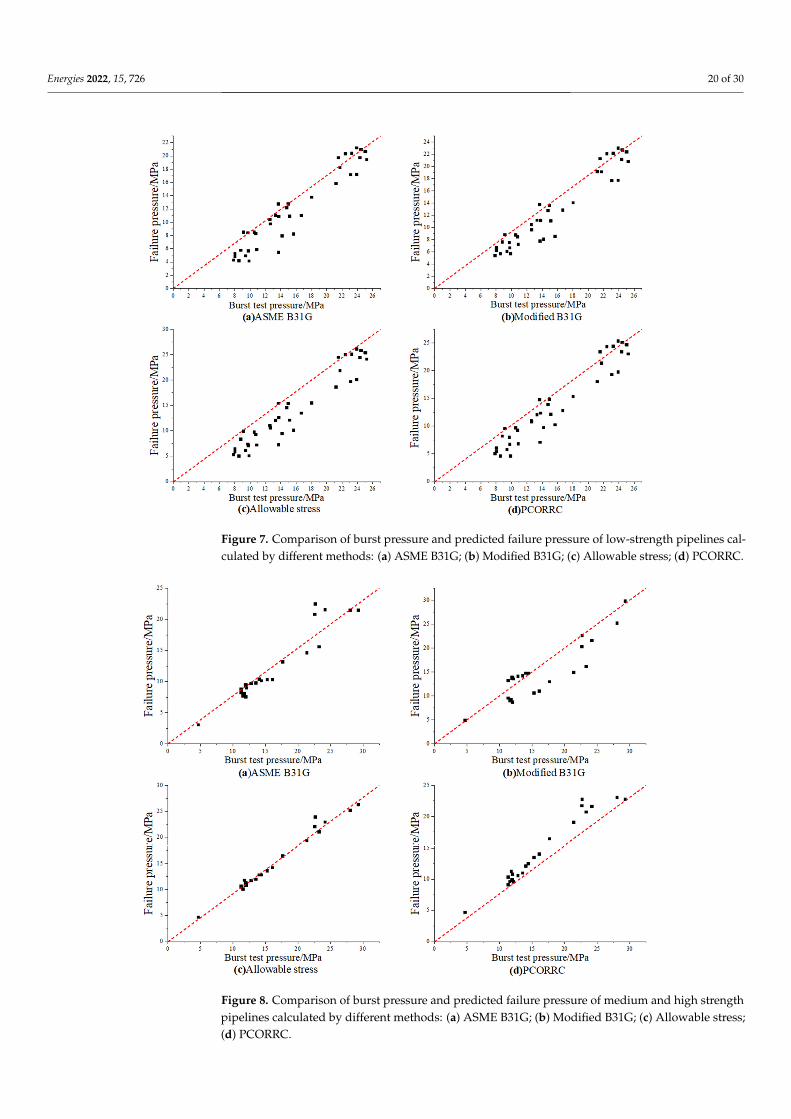
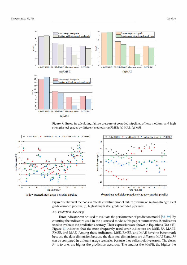
4.2. Result Analysis of Traditional Evaluation Methods Due to the differences in various evaluation methods in many aspects [54], the

calculation results also be affected. In all, 64 groups of data were collected from the literature [12], including 40 groups of low-strength steel grade corrosion pipes (X42, X46-1, X46-2, X46-3, X46-4, X52-1, X52-2, and X56) and 24 groups of medium and high-strength steel grade corrosion pipes (X60, X65, and X80), including defect size parameters, pipe size parameters, material parameters, and burst test pressure. The result analysis of various evaluation methods is shown in Figures 7–10. As the figures show, ASME B31G has large errors in evaluating whether it is a medium-to-high strength pipeline or a low-strength pipeline. The Modified B31G has improved significantly. When evaluating low-strength steel pipes, the DNV-RP-F101 allowable stress method and PCORRC have similar errors. However, when evaluating high-strength steel-grade pipelines, the accuracy of the DNV-RP-F101 allowable stress method is much higher than that of PCORRC.

Figure 6. The number of related intelligent models from 2011 to November 2021.

4.2. Result Analysis of Traditional Evaluation Methods

Due to the differences in various evaluation methods in many aspects [54], the calcula-tion results also be affected. In all, 64 groups of data were collected from the literature [12],including 40 groups of low-strength steel grade corrosion pipes (X42, X46-1, X46-2, X46-3,X46-4, X52-1, X52-2, and X56) and 24 groups of medium and high-strength steel gradecorrosion pipes (X60, X65, and X80), including defect size parameters, pipe size parameters,material parameters, and burst test pressure. The result analysis of various evaluationmethods is shown in Figures 7–10. As the figures show, ASME B31G has large errors inevaluating whether it is a medium-to-high strength pipeline or a low-strength pipeline.The Modified B31G has improved significantly. When evaluating low-strength steel pipes,the DNV-RP-F101 allowable stress method and PCORRC have similar errors. However,when evaluating high-strength steel-grade pipelines, the accuracy of the DNV-RP-F101allowable stress method is much higher than that of PCORRC.


Figure 7. Comparison of burst pressure and predicted failure pressure of low-strength pipelines calculated by different methods: (a) ASME B31G; (b) Modified B31G; (c) Allowable stress; (d) PCORRC.

Figure 8. Comparison of burst pressure and predicted failure pressure of medium and high strength pipelines calculated by different methods: (a) ASME B31G; (b) Modified B31G; (c) Allowable stress; (d) PCORRC.

Figure 7. Comparison of burst pressure and predicted failure pressure of low-strength pipelines cal-culated by different methods: (a) ASME B31G; (b) Modified B31G; (c) Allowable stress; (d) PCORRC.


Figure 7. Comparison of burst pressure and predicted failure pressure of low-strength pipelines calculated by different methods: (a) ASME B31G; (b) Modified B31G; (c) Allowable stress; (d) PCORRC.

Figure 8. Comparison of burst pressure and predicted failure pressure of medium and high strength pipelines calculated by different methods: (a) ASME B31G; (b) Modified B31G; (c) Allowable stress; (d) PCORRC.

Figure 8. Comparison of burst pressure and predicted failure pressure of medium and high strengthpipelines calculated by different methods: (a) ASME B31G; (b) Modified B31G; (c) Allowable stress;(d) PCORRC.


Figure 9. Errors in calculating failure pressure of corroded pipelines of low, medium, and high strength steel grades by different methods: (a) RMSE; (b) MAE; (c) MSE.

Figure 10. Different methods to calculate relative error of failure pressure of: (a) low-strength steel grade corroded pipeline; (b) high-strength steel grade corroded pipelines.

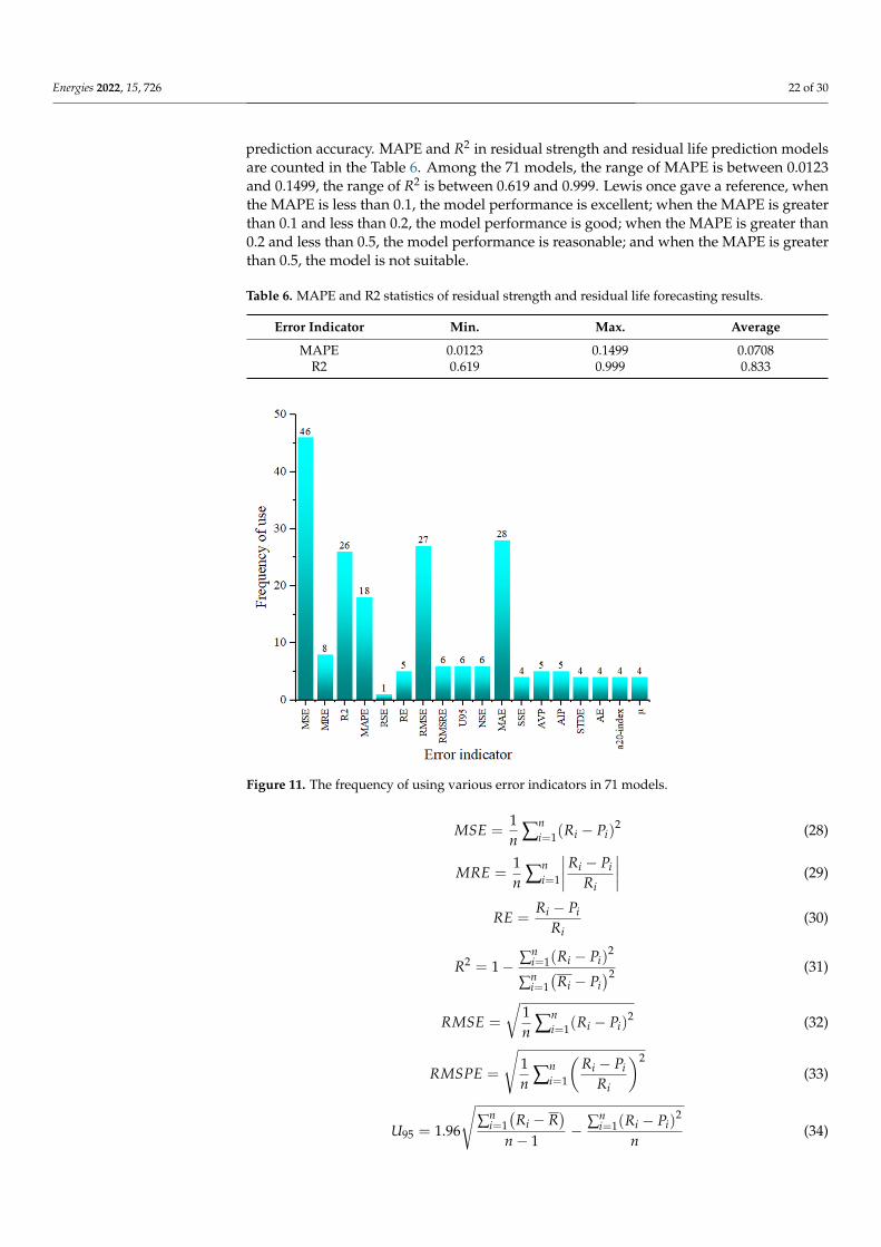
4.3. Prediction Accuracy Error indicator can be used to evaluate the performance of prediction model [55–59].

By counting the indicators used in the discussed models, this paper summarizes 18 indicators used to evaluate the prediction accuracy. Their expressions are shown in Equations (28)–(43), Figure 11 indicates that the most frequently used error indicators are MSE, R2, MAPE, RMSE, and MAE. Among these indicators, MSE, RMSE, and MAE have no benchmark because the data dimension because the data sets dimensions are different. MAPE and R2 can be compared in different usage scenarios because they reflect relative

Figure 9. Errors in calculating failure pressure of corroded pipelines of low, medium, and highstrength steel grades by different methods: (a) RMSE; (b) MAE; (c) MSE.


Figure 9. Errors in calculating failure pressure of corroded pipelines of low, medium, and high strength steel grades by different methods: (a) RMSE; (b) MAE; (c) MSE.

Figure 10. Different methods to calculate relative error of failure pressure of: (a) low-strength steel grade corroded pipeline; (b) high-strength steel grade corroded pipelines.

4.3. Prediction Accuracy Error indicator can be used to evaluate the performance of prediction model [55–59].

By counting the indicators used in the discussed models, this paper summarizes 18 indicators used to evaluate the prediction accuracy. Their expressions are shown in Equations (28)–(43), Figure 11 indicates that the most frequently used error indicators are MSE, R2, MAPE, RMSE, and MAE. Among these indicators, MSE, RMSE, and MAE have no benchmark because the data dimension because the data sets dimensions are different. MAPE and R2 can be compared in different usage scenarios because they reflect relative

Figure 10. Different methods to calculate relative error of failure pressure of: (a) low-strength steelgrade corroded pipeline; (b) high-strength steel grade corroded pipelines.

4.3. Prediction Accuracy

Error indicator can be used to evaluate the performance of prediction model [55–59]. Bycounting the indicators used in the discussed models, this paper summarizes 18 indicatorsused to evaluate the prediction accuracy. Their expressions are shown in Equations (28)–(43),Figure 11 indicates that the most frequently used error indicators are MSE, R2, MAPE,RMSE, and MAE. Among these indicators, MSE, RMSE, and MAE have no benchmarkbecause the data dimension because the data sets dimensions are different. MAPE and R2

can be compared in different usage scenarios because they reflect relative errors. The closerR2 is to one, the higher the prediction accuracy. The smaller the MAPE, the higher the

Energies 2022, 15, 726 22 of 30

prediction accuracy. MAPE and R2 in residual strength and residual life prediction modelsare counted in the Table 6. Among the 71 models, the range of MAPE is between 0.0123and 0.1499, the range of R2 is between 0.619 and 0.999. Lewis once gave a reference, whenthe MAPE is less than 0.1, the model performance is excellent; when the MAPE is greaterthan 0.1 and less than 0.2, the model performance is good; when the MAPE is greater than0.2 and less than 0.5, the model performance is reasonable; and when the MAPE is greaterthan 0.5, the model is not suitable.

Table 6. MAPE and R2 statistics of residual strength and residual life forecasting results.

Error Indicator Min. Max. Average

MAPE 0.0123 0.1499 0.0708R2 0.619 0.999 0.833


errors. The closer R2 is to one, the higher the prediction accuracy. The smaller the MAPE, the higher the prediction accuracy. MAPE and R2 in residual strength and residual life prediction models are counted in the Table 6. Among the 71 models, the range of MAPE is between 0.0123 and 0.1499, the range of R2 is between 0.619 and 0.999. Lewis once gave a reference, when the MAPE is less than 0.1, the model performance is excellent; when the MAPE is greater than 0.1 and less than 0.2, the model performance is good; when the MAPE is greater than 0.2 and less than 0.5, the model performance is reasonable; and when the MAPE is greater than 0.5, the model is not suitable.

Table 6. MAPE and R2 statistics of residual strength and residual life forecasting results.

Error Indicator Min. Max. Average MAPE 0.0123 0.1499 0.0708

R2 0.619 0.999 0.833

Figure 11. The frequency of using various error indicators in 71 models.

𝑀𝑆𝐸 = ∑ (𝑅 − 𝑃 ) (28)

𝑀𝑅𝐸 = ∑ (29)

𝑅𝐸 = 𝑅 − 𝑃𝑅 (30)

𝑅 = 1 − ∑ (𝑅 − 𝑃 )∑ 𝑅 − 𝑃 (31)

𝑅𝑀𝑆𝐸 = ∑ (𝑅 − 𝑃 ) (32)

𝑅𝑀𝑆𝑃𝐸 = ∑ (33)

Figure 11. The frequency of using various error indicators in 71 models.

MSE =1n ∑n

i=1(Ri − Pi)2 (28)

MRE =1n ∑n

i=1

∣∣∣∣Ri − PiRi

∣∣∣∣ (29)

RE =Ri − Pi

Ri(30)

R2 = 1− ∑ni=1(Ri − Pi)

2

∑ni=1(

Ri − Pi)2 (31)

RMSE =

√1n ∑n

i=1(Ri − Pi)2 (32)

RMSPE =

√1n ∑n

i=1

(Ri − Pi

Ri

)2(33)

U95 = 1.96

√∑n

i=1(

Ri − R)

n− 1− ∑n

i=1(Ri − Pi)2

n(34)

Energies 2022, 15, 726 23 of 30

NSE = 1− ∑ni=1(Ri − Pi)

2

∑ni=1(

Ri − Ri)2 (35)

MAE =1n ∑n

i=1|Ri − Pi| (36)

SSE = ∑ni=1(Ri − Pi)

2 (37)

AIP =100%

n

n

∑i=1

∣∣∣∣1− PiRi

∣∣∣∣ (38)

AVP = 1− AIP (39)

STDE = std(Ri − Pi) (40)

AE = |Ri − Pi| (41)

a20− index =er20

n(42)

µ =1n ∑n

i=1PiRi

(43)

4.4. Data Size and Data Division

Data size is one of the main factors affecting forecasting performance. Too much datawill lead to too much calculation, while too little data may lead to the insufficient modelaccuracy. Table 7 provides statistical information on the data size of 71 smart models, whichcan provide a basis for selecting data sizes in subsequent studies. The original data areusually divided into three data sets in machine learning, including training set, validationset, and test set. The training set is used to train the model; the validation set data are usedto adjust the parameters of the training model; and the test set data are used to measure theperformance of the training model. However, only 2 of the 71 models divide the originaldata into three data sets, and the remaining 69 models only divide it into the training andtest sets (Figure 12). The proportion of test set is in the range of 0.015–0.4.


Figure 12. Division proportion of raw data.

4.5. Input Variable and Output Value In the intelligent model, how to determine the input variables is a very critical issue

[60,61]. Therefore, in the remaining strength and remaining life prediction model, it is necessary to consider which factors are used as input variables fully. According to the input variables, it can be divided into two categories. One is to simply use certain historical data as input variables to predict the future trend of the variable, such as using the historical wall thickness of the pipeline to predict the remaining wall thickness or using the historical corrosion rate to predict the future corrosion rate. The other is the prediction that considers multiple factors, such as predicting the burst pressure of the pipeline through pipeline size parameters, defect parameters, environmental parameters, and material parameters (Table 8). The former is simple to calculate, and convenient to obtain data, but the prediction accuracy is not necessarily high, because this type of prediction assumes that external factors are stable. The latter is difficult to obtain data, and needs to consider the nonlinear relationship of multiple variables, but the prediction results are often more comprehensive and accurate. According to the statics of the models compiled in this paper, 10 of the 71 models are simple time-series predictions, and the rest are forecasting considering multiple factors.

Table 8. The input variables of prediction models.

Input Variables Type Parameters

Environmental factor

P, UL, TM, SR, ORP, PCO2, TAUWWT, TAUWG, PP, RP, BD, CC, OP, BSW, GSG, GPR, OPR, WPR, AW, CP, CG, JC, FS, ML,

SUP, HTK, USG, BP, EM, STC, OC, pH, SC, WC, SEC, HOL, DC, BC, CMC, SEC

Corrosion Defect data l, w, d Pipe data D, WT Material UTS, YS, TS, EM, BP, Pipe steel grade Others T, CR

Figure 12. Division proportion of raw data.

Energies 2022, 15, 726 24 of 30

Table 7. The data size of prediction models.

Burst Pressure Remaining Thickness Corrosion Rate Corrosion DefectDepth Others

Max. Min. Mean Max. Min. Mean Max. Min. Mean Max. Min. Mean Max. Min. Mean

453 15 167 259 15 188 60 15 43 3250 60 2612 4990 30 2171

4.5. Input Variable and Output Value

In the intelligent model, how to determine the input variables is a very criticalissue [60,61]. Therefore, in the remaining strength and remaining life prediction model, it isnecessary to consider which factors are used as input variables fully. According to the inputvariables, it can be divided into two categories. One is to simply use certain historical dataas input variables to predict the future trend of the variable, such as using the historicalwall thickness of the pipeline to predict the remaining wall thickness or using the historicalcorrosion rate to predict the future corrosion rate. The other is the prediction that considersmultiple factors, such as predicting the burst pressure of the pipeline through pipelinesize parameters, defect parameters, environmental parameters, and material parameters(Table 8). The former is simple to calculate, and convenient to obtain data, but the predic-tion accuracy is not necessarily high, because this type of prediction assumes that externalfactors are stable. The latter is difficult to obtain data, and needs to consider the nonlinearrelationship of multiple variables, but the prediction results are often more comprehen-sive and accurate. According to the statics of the models compiled in this paper, 10 ofthe 71 models are simple time-series predictions, and the rest are forecasting consideringmultiple factors.

Table 8. The input variables of prediction models.

Input Variables Type Parameters

Environmental factor

P, UL, TM, SR, ORP, PCO2, TAUWWT,TAUWG, PP, RP, BD, CC, OP, BSW, GSG, GPR,OPR, WPR, AW, CP, CG, JC, FS, ML, SUP, HTK,

USG, BP, EM, STC, OC, pH, SC, WC, SEC,HOL, DC, BC, CMC, SEC

Corrosion Defect data l, w, d

Pipe data D, WT

Material UTS, YS, TS, EM, BP, Pipe steel grade

Others T, CR

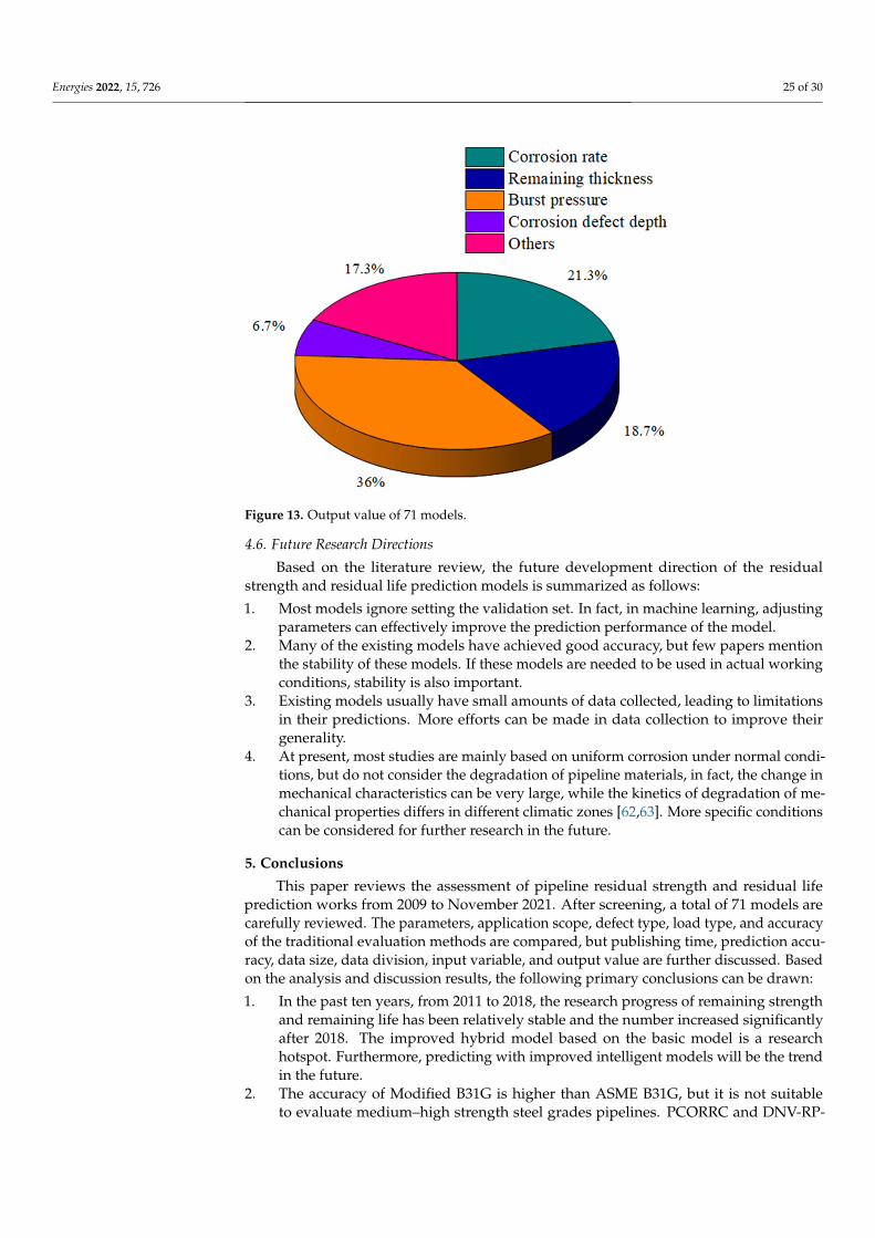
The prediction targets of these models can be roughly divided into the following fourcategories: burst pressure, remaining thickness, corrosion rate, and others. Among them,burst pressure accounts for 36%, remaining thickness accounts for 18.7%, corrosion rateaccounts for 21.3%, corrosion defect depth accounts for 6.7%, and the others accounts for17.3%. The proportion of each item is shown in Figure 13. It can be seen from Figure 13that the model with burst pressure as the output value is still the most, the rest are similar.

Energies 2022, 15, 726 25 of 30


The prediction targets of these models can be roughly divided into the following four categories: burst pressure, remaining thickness, corrosion rate, and others. Among them, burst pressure accounts for 36%, remaining thickness accounts for 18.7%, corrosion rate accounts for 21.3%, corrosion defect depth accounts for 6.7%, and the others accounts for 17.3%. The proportion of each item is shown in Figure 13. It can be seen from Figure 13 that the model with burst pressure as the output value is still the most, the rest are similar.

Figure 13. Output value of 71 models.

4.6. Future Research Directions Based on the literature review, the future development direction of the residual

strength and residual life prediction models is summarized as follows: 1. Most models ignore setting the validation set. In fact, in machine learning, adjusting

parameters can effectively improve the prediction performance of the model. 2. Many of the existing models have achieved good accuracy, but few papers mention

the stability of these models. If these models are needed to be used in actual working conditions, stability is also important.

3. Existing models usually have small amounts of data collected, leading to limitations in their predictions. More efforts can be made in data collection to improve their generality.

4. At present, most studies are mainly based on uniform corrosion under normal conditions, but do not consider the degradation of pipeline materials, in fact, the change in mechanical characteristics can be very large, while the kinetics of degradation of mechanical properties differs in different climatic zones [62,63]. More specific conditions can be considered for further research in the future.

5. Conclusions This paper reviews the assessment of pipeline residual strength and residual life

prediction works from 2009 to November 2021. After screening, a total of 71 models are carefully reviewed. The parameters, application scope, defect type, load type, and accuracy of the traditional evaluation methods are compared, but publishing time, prediction accuracy, data size, data division, input variable, and output value are further

Figure 13. Output value of 71 models.

4.6. Future Research Directions

Based on the literature review, the future development direction of the residualstrength and residual life prediction models is summarized as follows:

1. Most models ignore setting the validation set. In fact, in machine learning, adjustingparameters can effectively improve the prediction performance of the model.

2. Many of the existing models have achieved good accuracy, but few papers mentionthe stability of these models. If these models are needed to be used in actual workingconditions, stability is also important.

3. Existing models usually have small amounts of data collected, leading to limitationsin their predictions. More efforts can be made in data collection to improve theirgenerality.

4. At present, most studies are mainly based on uniform corrosion under normal condi-tions, but do not consider the degradation of pipeline materials, in fact, the change inmechanical characteristics can be very large, while the kinetics of degradation of me-chanical properties differs in different climatic zones [62,63]. More specific conditionscan be considered for further research in the future.

5. Conclusions

This paper reviews the assessment of pipeline residual strength and residual lifeprediction works from 2009 to November 2021. After screening, a total of 71 models arecarefully reviewed. The parameters, application scope, defect type, load type, and accuracyof the traditional evaluation methods are compared, but publishing time, prediction accu-racy, data size, data division, input variable, and output value are further discussed. Basedon the analysis and discussion results, the following primary conclusions can be drawn:

1. In the past ten years, from 2011 to 2018, the research progress of remaining strengthand remaining life has been relatively stable and the number increased significantlyafter 2018. The improved hybrid model based on the basic model is a researchhotspot. Furthermore, predicting with improved intelligent models will be the trendin the future.

2. The accuracy of Modified B31G is higher than ASME B31G, but it is not suitableto evaluate medium–high strength steel grades pipelines. PCORRC and DNV-RP-

Energies 2022, 15, 726 26 of 30

F101 are similar in evaluating low strength pipelines, and DNV-RP-F101 has a betterperformance in evaluating medium–high strength pipelines.

3. The most frequently used error indicators are MSE, R2, MAPE, RMSE, and MAE.Among them, MAPE is in the range of 0.0123–0.1499; R2 is in the range of 0.619–0.999.

4. The proportion of test data set is between 0.015 and 0.4, and only 2 of 71 models areusing the validation set. In fact, correctly setting the proportion of data can furtherimprove the prediction accuracy and achieve better results. Researchers also need topay more attention to this aspect.

5. Models are divided into considering a single variable in the time series, and consider-ing multiple factors based on input variables. There are 61 of 71 models in this paperconsidering multiple factors. These models can be divided into four main categoriesbased on output value. Among them, burst pressure accounts for 36%, remainingthickness accounts for 18.7%, corrosion rate accounts for 21.3%, corrosion defect depthaccounts for 6.7%, and the others accounts for 17.3%.

Author Contributions: Conceptualization, H.L.; formal analysis, H.L.; investigation, H.L.; resources,Q.Z.; writing—original draft preparation, H.L.; writing—review and editing, K.H.; visualization, C.S.;supervision, K.H. All authors have read and agreed to the published version of the manuscript.

Funding: This research received no external funding.

Institutional Review Board Statement: Not applicable.

Informed Consent Statement: Not applicable.

Data Availability Statement: Not applicable.

Acknowledgments: Thanks to Lu Hongfang for his careful guidance during the writing of the thesis.

Conflicts of Interest: The authors declare no conflict of interest.

Nomenclature

A Projected area of defect on axial through wall planeA* The triangular fuzzy numberA0 Cross sectional area of original pipe wall at defecta20-index er20/ner20 Number of samples whose absolute error is less than 20%M Folias Bulging Coefficientn Sample sizefu Tensile strength (considering temperature reduction effect)Pf The residual strength of the pipePi Prediction value at time kR2 Goodness of FitRi Real value at time istd Population standard deviationU95 The confidence level of the expanded uncertainty is 95%σflow The flow stressσu The tensile strength of the pipeεd Quantile coefficient of defect depthγm Partial safety factorγd Defect depth safety factor(d/t) * (d/t) meas + εd·std (d/t)(d/t) meas Measured value of defect depth ratioAbbreviationsAE Average ErrorAGA American National Gas AssociationAIP Average Invalidity PercentANN Artificial Neural NetworkANP Analytic Network Process

Energies 2022, 15, 726 27 of 30

ASME American Society of Mechanical EngineersAVP Average Validity PercentAW Anode WastageBC BicarbonateBD Bulk DensityBG British Gas CompanyBP Burst PressureBPNN Back Propagation Neural NetworkBSW Basic Sediments and WaterBWNN B-spline Wavelet Neural NetworkCC Coating ConditionCDD Corrosion Defect DepthCG CrossingsCMC Calcium/Magnesium ion ContentCP Cathodic ProtectionCR Corrosion RateCS Cuckoo SearchCV Cross Validationd The depth of corrosion defectD Pipe DiameterDC Dissolved ChlorideDNN Deep Neural NetworksDNV DET NORSKE VERITASEGIG European Gas Pipeline Incident Data GroupELM Extreme Learning MachinesEM Elastic ModulusFS Free SpansFSM Field Signature MethodFSNN Fuzzy Surfacelet Neural NetworkGA Genetic AlgorithmGBDT Gradient Boosting Decision TreeGBM Gradient Boosting MachineGM(1,1) First Order Univariate Gray System ModelGPR Gas Production RateGRNN General Regression Neural NetworkGSG Gas Specific GravityHOL Liquid HoldupHTK Heat Transfer Coefficient of Inner wallIDA Improved Dragonfly AlgorithmIPSA Improved Particle Swarm AlgorithmJC Joint ConditionKR Krigingl the length of corrosion defectLWP Locally Weighted PolynomialsMAE Mean Absolute ErrorMAPE Mean Absolute Percentage ErrorMARS Multivariate Adaptive Regression SplinesML Metal LossMOGWO Multiobjective Grey Wolf OptimizationMRE Mean Relative ErrorMSE Mean Square ErrorNSE Nash-Sutcliffe EfficiencyNSGA Nondominated Sorting Genetic AlgorithmOC Oxygen ContentOP Operating PressureOPR Oil Production RateORP Oxidation-reduction potentialP Pressure

Energies 2022, 15, 726 28 of 30

PCA Principal Component AnalysisPCO2 Partial Pressure of CO2PCORRC Pipeline Corrosion CriterionPP Pipe-to-soil PotentialPSID Deposition RatePSO Particle Swarm OptimizationPSO Particle Swarm OptimizerRBF Radial Basis FunctionRE Relative ErrorRF Random ForestRMSE Root Mean Square ErrorRMSRE Root Mean Squared Relative ErrorRP Redox PotentialRS Rough SetSC Sulfate ion ConcentrationsSEC Stray Electric CurrentSGD Stochastic Gradient DescentSR Soil resistivitySSCN Subspace Clustered Neural NetworkSSE Error Sum of SquaresSMTS The material tensile limitSMYS The minimum yield stressSTC Salt ContentSTDE Population standard deviation of errorSUP Support ConditionSVM Support Vector MachineSVR Support Vector RegressionT Time(years)TAUWG Wall shear stress (gas phase)TAUWHL Liquid-maximum wall shear stressTAUWWT Wall shear stress (liquid phase)TDA Traditional Dragonfly AlgorithmTM TemperatureUL Liquid flow rateUSG Superficial Velocity GasUTS Ultimate Tensile Strengthw The width of corrosion defectWC Water ContentWNN Weighted nearest neighborWPR Water Production RateWT Wall ThicknessYS Yield Strength

References1. EGIG. Available online: https://www.egig.eu/reports (accessed on 19 October 2021).2. Lyons, C.J.; Race, J.M.; Chang, E.; Cosham, A.; Barnett, J. Validation of the ng-18 equations for thick walled pipelines. EFA 2020,

112, 104494. [CrossRef]3. The American Society of Mechanical Engineers. Manual for Determining the Remaining Strength of Corroded Pipelines; ASME:

New York, NY, USA, 1984; pp. 1–38.4. The American Society of Mechanical Engineers. Manual for Determining the Remaining Strength of Corroded Pipelines; ASME:

New York, NY, USA, 1991; pp. 1–47.5. Kiefner, J.F.; Vieth, P.H. A Modified Criterion for Evaluating the Remaining Strength of Corroded Pipe; Pipeline Research Committee,

American Gas Association: Washington, DC, USA, 1989.6. Ma, B.; Jian, S.; Wang, J.; Han, K. Analysis on the latest assessment criteria of ASME b31g-2009 for the remaining strength of

corroded pipelines. JFAP 2011, 11, 666–671. [CrossRef]7. Ma, B.; Shuai, J.; Li, X.; Wang, J.; Feng, Q. Advances in the newest version of ASME b31g-2009. NGI 2011, 31, 112–115.8. Veritas, D.N. Corroded Pipelines; RP, 2004; p. 11. Available online: http://opimsoft.com/download/reference/rp-f101_2006-10

.pdf (accessed on 19 October 2021).

https://www.egig.eu/reports

http://doi.org/10.1016/j.engfailanal.2020.104494

http://doi.org/10.1007/s11668-011-9490-8

http://opimsoft.com/download/reference/rp-f101_2006-10.pdf

http://opimsoft.com/download/reference/rp-f101_2006-10.pdf

Energies 2022, 15, 726 29 of 30

9. Xiao, K.; Liu, Y.; Wang, L.; Qian, Y. A Study on Assessment Methods for the Remaining Strength of Corroded Pipelines; GCI: Anchorage,AK, USA, 2013.

10. Stephens, D.R.; Leis, B.N.; Kurre, M.D.; Rudland, D.L. Development of an alternative criterion for residual strength of corrosiondefects in moderate-to high-toughness pipe. In Proceedings of the 2000 International Pipeline Conference, Calgary, AB, Canada,1–5 October 2000.

11. Tomar, M.S.; Fingerhut, M. Reliable application of rstreng criteria for in-the-ditch assessment of corrosion defects in transmissionpipelines. NACE Int. Corros. Conf. Ser. 2006, 176, 1–8.

12. Wang, L.B. Development of Software for Residual Strength Evaluation and Residual Life Prediction of Corroded Pipelines.Master’s Thesis, Xi’an Shiyou University, Xi’an, China, 2014.

13. Hua, C. Contrastive Study on New and Old Evaluation Standards of SY/T 6151 for Corrosion Pipeline. CCI 2016, 45, 1476–1479.14. Chen, Z.; Wu, M.; Xie, F.; Wang, D.; Guo, Q.; Ma, F. Evaluation method and remaining life prediction of corroded pipeline residual

strength. MEM 2015, 5, 97–101.15. Rosenblatt, F. The perceptron: A probabilistic model for information storage and organization in the brain. Psychol. Rev. 1958, 65,

386–408. [CrossRef] [PubMed]16. Katz, W.T.; Snell, J.W.; Merickel, M.B. Artificial neural networks. Methods Enzymol. 1992, 210, 610–636.17. Rahmanifard, H.; Plaksina, T. Application of artificial intelligence techniques in the petroleum industry: A review. Artif. Intell.

Rev. 2019, 52, 2295–2318. [CrossRef]18. Zhao, Y.; Zhao, B. Research on pressure pipeline explosion based on triangular fuzzy mathematics and fault tree analysis. JLUPCT

2018, 6, 65–69.19. Wind, Y.; Saaty, T. Marketing Applications of the Analytic Hierarchy Process. Manag. Sci. 1980, 26, 641–658. [CrossRef]20. Liang, Q. Pressure pipeline leakage risk research based on trapezoidal membership degree fuzzy mathematics. GST 2019, 24,

48–53.21. Lorenz, E.N. Deterministic nonperiodic flow. SNY 1963, 20, 130–141. [CrossRef]22. Hunt, B.R.; Li, T.Y.; Kennedy, J.A.; Nusse, H.E. Period three implies chaos. SNY 2004, 6, 77–84.23. Cortes, C.; Vapnik, V.; Llorens, C. Support-vector networks. Mach. Learn. 1995, 20, 273–297. [CrossRef]24. Liu, H.; Liu, D.; Zheng, G.; Liang, Y. Research on natural gas short term load forecasting based on support vector expression.

Chin. J. Chem. Eng. 2004, 12, 5.25. Qu, C. Study on Residual Life Prediction METHOD of Corrosive Defective Pipeline. Master’s Thesis, Northeast University,

Shenyang, China, 2014.26. Yan, J. Study on Prediction and Evaluation Method of Inner WALL corrosion of SUBMARINE pipeline. Master’s Thesis, Dalian

University of Technology, Dalian, China, 2020.27. Qin, X.; Liu, W.; Chen, L. Pipeline corrosion prediction based on improved bee colony algorithm and grey model. J. Beijing Univ.

Chem. Technol. 2021, 48, 74–80.28. Wang, W.H. Corrosion Rate Prediction and Residual Life Research of Buried Oil and Gas Pipelines. Master’s Thesis, Xi’an

University of Architecture and Technology, Xi’an, China, 2019.29. Cheng, X. Study on Corrosion Residual Life Prediction of Buried Gas PIPELINE Based on Comprehensive Detection. Master’s

Thesis, South China University of Technology, Guangzhou, China, 2016.30. Peng, S.; Zhang, Z.; Liu, E.; Liu, W.; Qiao, W. A new hybrid algorithm model for prediction of internal corrosion rate of multiphase

pipeline. J. Nat. Gas. Sci. Eng. 2021, 85, 103716. [CrossRef]31. Ben Seghier, M.E.A.; Keshtegar, B.; Taleb-Berrouane, M.; Abbassi, R.; Trung, N. Advanced intelligence frameworks for predicting

maximum pitting corrosion depth in oil and gas pipelines. Process Saf. Environ. 2021, 147, 818–833. [CrossRef]32. Ossai, C.I. Corrosion defect modelling of aged pipelines with a feed-forward multi-layer neural network for leak and burst failure

estimation. Eng. Fail. Anal. 2020, 110, 104397. [CrossRef]33. Sun, J.; Zhao, B.; Gao, D.; Xu, L. Fuzzy surfacelet neural network evaluation model optimized by adaptive dragonfly algorithm

for pipeline network integrity management. Appl. Soft. Comput. 2021, 113, 107862. [CrossRef]34. Zhang, T.; Zhou, L. Combining Forecasting Model of Pipeline’s Corrosion Rate Based on Artificial Immune Algorithm. In

Proceedings of the International Conference on Pipelines and Trenchless, Wuhan, China, 19–22 October 2012.35. El-Abbasy, M.S.; Senouci, A.; Zayed, T.; Mirahadi, F.; Parvizsedghy, L. Condition Prediction Models for Oil and Gas Pipelines

Using Regression Analysis. J. Constr. Eng. Manag. 2014, 140. [CrossRef]36. Luo, Z.; Hu, X.; Gao, Y. Corrosion research of wet natural gathering and transportation pipeline based on SVM. In Proceedings of

the International Conference on Pipelines and Trenchless, Xi’an, China, 16–18 October 2013.37. Lu, H.; Xu, Z.D.; Iseley, T.; Matthews, J.C. Novel Data-Driven Framework for Predicting Residual Strength of Corroded Pipelines.

J. Pipeline Syst. Eng. 2021, 12, 04021045. [CrossRef]38. Zheng, Y.; Shu, J.; Ren, C.; Zhang, F. Prediction of Gathering Pipeline Internal Corrosion Rate Based on Improved Wavelet

Neural Network Model. In Proceedings of the International Conference on Pipelines and Trenchless Technology, Beijing, China,26–29 October 2011.

39. Sun, B.C.; Li, S.X.; Yu, S.R.; Zeng, H.L. Improved BP algorithm to predict the residual strength of corroded pipelines. CJCP 2011,5, 404–408.

http://doi.org/10.1037/h0042519

http://www.ncbi.nlm.nih.gov/pubmed/13602029

http://doi.org/10.1007/s10462-018-9612-8

http://doi.org/10.1287/mnsc.26.7.641

http://doi.org/10.1175/1520-0469(1963)020<0130:DNF>2.0.CO;2

http://doi.org/10.1007/BF00994018

http://doi.org/10.1016/j.jngse.2020.103716

http://doi.org/10.1016/j.psep.2021.01.008

http://doi.org/10.1016/j.engfailanal.2020.104397

http://doi.org/10.1016/j.asoc.2021.107862

http://doi.org/10.1061/(ASCE)CO.1943-7862.0000838

http://doi.org/10.1061/(ASCE)PS.1949-1204.0000587

Energies 2022, 15, 726 30 of 30

40. Sharifi, M.; Yao, K.T.; Raghavendra, S.; Ershaghi, I.; House, R.; Blouin, J. Prediction of Remaining Life in Pipes using MachineLearning from Thickness Measurements. In Proceedings of the SPE Western Regional Meeting, Garden Grove, CA, USA,27–30 April 2015.

41. Hou, P.P. Research on the Influence of Corrosion Defects on the Residual Strength of Oil and Gas Pipelines. Master’s Thesis,Xinjiang University, Xinjiang, China, 2017.

42. Sun, B.C.; Wu, J.W.; Li, L.; She, Z.G. Improved GA-BP algorithm for oil and gas pipeline corrosion residual strength prediction.JSPU Nat. Sci. Ed. 2013, 3, 160–167.

43. Ma, S.; Li, J.F.; Bai, R.; Dai, Z. Prediction of residual strength of oil and gas pipelines based on PCA-SVR model. OGST 2019, 10,1119–1124.

44. Wang, W.H.; Luo, Z.S.; Zhang, X.S. Prediction of buried pipeline corrosion remaining life based on PSO-GRNN model. Surf.Technol. 2019, 10, 267–275.

45. Yang, X.D.; Zhou, Y.L.; Liu, Z.J.; Lu, L.; Yu, T.Q.; Liu, Y. Research on residual strength prediction technology of corroded pipelinebased on RS-PSO-SVM algorithm. PEC 2020, 3, 8–12.

46. Xie, P.; Liu, H.; Gong, Y.H.; Ni, P.P.; Heman, A. Evaluation of residual strength of external corrosion of submarine pipelines basedon deep learning. OGST 2021, 6, 651–657.

47. Luo, Z.S.; Yuan, H.W. GM-RBF submarine pipeline corrosion prediction model based on error compensation. CJSS 2018, 3, 96–101.48. Ma, G. Residual Strength Prediction of Single-Defect Pipeline Based on Correlation Analysis and SVM Algorithm. Master’s

Thesis, Xi’an Petroleum University, Xi’an, China, 2020.49. Li, J.G.; Lin, S.J.; Long, W.; Xu, L. Prediction of remaining life of metal pipes in uniform corrosion based on FSM non-destructive

testing. Surf. Technol. 2016, 3, 7–11.50. Li, Q.; Sun, C.M.; Huang, Z.Q.; Xiao, X.; Tang, H.P. Combined forecasting method of GA-BP neural network for failure pressure

of Lan-Cheng-Yu corroded pipelines. OJSST 2015, 11, 83–89.51. Zhang, Y. Research on Residual Strength of Multipoint Corrosion Defective Pipeline Based on Finite Element and PSO-BP.

Master’s Thesis, Xi’an University of Architecture and Technology, Xi’an, China, 2020.52. Bi, A.R.; Luo, Z.S.; Song, Y.Y.; Zhang, X.S. Residual strength analysis of internally corroded submarine pipeline based on

FOA-GRNN model. CSSJ 2020, 6, 78–83.53. Jia, S.Q.; Qie, Y.H.; Li, Y.T.; Li, N.N. Research on burst pressure prediction of oil and gas pipelines with uniform corrosion defects

based on GA-BPNNs algorithm. JSST 2020, 12, 105–110.54. Syrotyuk, A.; Vytyaz, O.; Ziaja, J. Damage to flexible pipes of coiled tubing equipment due to corrosion and fatigue: Methods and

approaches for evaluation. Min. Mineral. Depos. 2017, 11, 96–103. [CrossRef]55. Lu, H.; Iseley, T.; Matthews, J.; Liao, W.; Azimi, M. An ensemble model based on relevance vector machine and multi-objective

salp swarm algorithm for predicting burst pressure of corroded pipelines. J. Petrol. Sci. Eng. 2021, 203, 108585. [CrossRef]56. Xu, Z.D.; Zhu, C.; Shao, L.W. Damage identification of pipeline based on ultrasonic guided wave and wavelet denoising. J.

Pipeline Syst. Eng. 2021, 12, 04021051. [CrossRef]57. Lu, H.; Iseley, T.; Matthews, J.; Liao, W. Hybrid machine learning for pullback force forecasting during horizontal directional

drilling. Automat. Constr. 2021, 129, 103810. [CrossRef]58. Xu, Z.D.; Yang, Y.; Miao, A.N. Dynamic Analysis and Parameter Optimization of Pipelines with Multidimensional Vibration

Isolation and Mitigation Device. J. Pipeline Syst. Eng. 2021, 12, 04020058. [CrossRef]59. Lu, H.; Matthews, J.C.; Azimi, M.; Iseley, T. Near Real-Time HDD Pullback Force Prediction Model Based on Improved Radial

Basis Function Neural Networks. J. Pipeline Syst. Eng. 2020, 11, 04020042. [CrossRef]60. Peng, S.; Chen, R.; Yu, B.; Xiang, M.; Lin, X.; Liu, E.E. Daily natural gas load forecasting based on the combination of long short

term memory, local mean decomposition, and wavelet threshold denoising algorithm. J. Nat. Gas. Sci. Eng. 2021, 95, 104175.[CrossRef]

61. Lu, H.; Behbahani, S.; Ma, X.; Iseley, T. A multi-objective optimizer-based model for predicting composite material properties.Constr. Build. Mater. 2021, 284, 122746. [CrossRef]

62. Maruschak, P.; Prentkovskis, O.; Bishchak, R. Defectiveness of external and internal surfaces of the main oil and gas pipelinesafter long-term operation. J. Civil. Eng. Manag. 2016, 22, 279–286. [CrossRef]

63. Panin, S.; Maruschak, P.; Vlasov, I.; Syromyatnikova, A.; Bolshakov, A.; Berto, F.; Prentkovskis, O.; Ovechkin, B. Effect of OperatingDegradation in Arctic Conditions on Physical and Mechanical Properties of 09Mn2Si Pipeline Steel. Procedia Eng. 2017, 178,597–603. [CrossRef]

http://doi.org/10.15407/mining11.04.096

http://doi.org/10.1016/j.petrol.2021.108585


http://doi.org/10.1016/j.autcon.2021.103810



http://doi.org/10.1016/j.jngse.2021.104175

http://doi.org/10.1016/j.conbuildmat.2021.122746

http://doi.org/10.3846/13923730.2015.1100672

http://doi.org/10.1016/j.proeng.2017.01.117

Documents

Residual Strength Assessment and Residual Life Prediction of