Response to Reviewer #1’s Comments

Anonymous Referee #1:

The authors presented a set of valuable data and conducted a meaningful analysis of the data. I

have a few comments, which may help improve clarity in some places. I don’t view that it is

reviewers’ responsibility to copy-edit and hence I did not point out all grammatical errors, but the

manuscript needs careful editing.

We sincerely appreciate the reviewer’s valuable comments and helpful suggestions on this

manuscript. We have carefully checked the grammar, syntax and semantic of all languages

throughout the manuscript based on the reviewer’s suggestions. We have responded to all the

comments point-by-point and made corresponding changes in the revised manuscript as

highlighted in red color. Please check the detailed responses to all the comments as below. The

reviewer’s comments are in black and our replies are in blue.

(1) Some of the results need to be quantitative. For instance, in the abstract, how much higher

were GEM and RGM concentrations in the northern SCS, Hgp2.5 and Hgp10 in PRE than

other areas (lines 48 -50)? How much higher were RGM concentrations during the day than at

night (lines 54 -56)? How much higher were their GEM concentrations than “those

background sites in the southern hemisphere” (lines 232-233) and “remote oceans” (lines

234-235)? How much higher were the GEM concentrations over the northern SCS from a

previous studies (lines 238-240)? They need to be quantitative about such comparisons.

Response:

We agree with the reviewer that the results should be quantitative. The concrete data has been

added in the revised manuscript.

See the revised manuscript at lines 19-29, 210-218, 295, 422-423, 427-428.

(2) Lines 81 – 88: Ye et al. (2016, acp) would be a good reference to cite, because their box model

included the most up-to-date gas-phase reactions of Hg and Br and simulated contributions

from variation oxidation reactions to GEM oxidation.

Response:

Thanks for the reviewer’s suggestions. We have made a careful study on the paper of

“Investigation of processes controlling summertime gaseous elemental mercury oxidation at

midlatitudinal marine, coastal, and inland sites”. The reference has been added in the revised

manuscript (lines 57-59, 62-65, 91, 750-752).

Reference:

Ye, Z., Mao, H., Lin, C.-J., and Kim, S. Y.: Investigation of processes controlling summertime

gaseous elemental mercury oxidation at midlatitudinal marine, coastal, and inland sites, Atmos.

Chem. Phys., 16, 84618478, https://doi.org/10.5194/acp-16-8461-2016, 2016.

(3) Line 97 – 102: Grammatical errors. They might want to break this rambling passage to three

sentences.

Response:

Thanks for your suggestion. This sentence has been divided into three sentences, which has

been revised as “The atmospheric reactive Hg deposited to the oceans follows different

reaction pathways. One important process is that divalent Hg can be combined with the

existing particles followed by sedimentation, or be converted to methylmercury (MeHg), the

most bioaccumulative and toxic form of Hg in seafood (Ahn et al., 2010; Mason et al., 2017).

Another important process is that the divalent Hg can be converted to dissolved gaseous Hg

(DGM) through abiotic and biotic mechanisms (Strode et al., 2007).” in the revised

manuscript.

Moreover, a section heading (3.5 Relationship between atmospheric Hg and meteorological

parameters) has been added in the revised manuscript to make the structure of the manuscript

clearer.

See the revised manuscript at lines 74-79, 401, 421.

(4) Lines 103 – 108: Too many excess articles. In fact, this was fairly commonly throughout the

text. They might want to give it a good editing to get rid of those excess articles.

Response:

Thanks for the suggestion. We have checked all the references throughout the manuscript, and

deleted those old and weakly related articles.

(5) Line 115: Mao et al. (2016, acp) provided a fairly complete review of the literature, up to early

2016, on spatiotemporal distributions of GEM, GOM, and PBM in different environments

worldwide, including coastal areas. Not just these four studies for reference.

Response:

Thanks for your comments. We have read carefully the paper of “Current understanding of the

driving mechanisms for spatiotemporal variations of atmospheric speciated mercury: a review”.

The related references (Ye et al., 2016 and Mao et al., 2016, 2017) have been added in the

revised manuscript.

See the revised manuscript at lines 91-92.

References:

1) Ye, Z., Mao, H., Lin, C.-J., and Kim, S. Y.: Investigation of processes controlling

summertime gaseous elemental mercury oxidation at midlatitudinal marine, coastal, and

inland sites, Atmos. Chem. Phys., 16, 84618478,

https://doi.org/10.5194/acp-16-8461-2016, 2016.

2) Mao, H., Cheng, I., and Zhang, L.: Current understanding of the driving mechanisms for

spatiotemporal variations of atmospheric speciated mercury: a review, Atmos. Chem.

Phys., 16, 1289712924, https://doi.org/10.5194/acp-16-12897-2016, 2016.

3) Mao, H., Hall, D., Ye, Z., Zhou, Y., Felton, D., and Zhang, L.: Impacts of large-scale

circulation on urban ambient concentrations of gaseous elemental mercury in New York,

USA, Atmos. Chem. Phys., 17, 1165511671, https://doi.org/10.5194/acp-17-11655-2017,

2017.

(6) Lines 258-259: The larger variabilities in RGM and Hgp were due not only to scavenging but

also likely due to their sensitivity to meteorological conditions and chemical environments.

Response:

Thanks for the insightful comments and we do agree with the reviewer’s comments. Thus, this

sentence has been revised as “indicating that atmospheric reactive Hg was easily scavenged

from the marine atmosphere due not only to their characteristics (high activity and solubility)

but also due to their sensitivity to meteorological conditions and chemical environments” in

the revised manuscript.

See the revised manuscript at lines 237-239.

(7) Figure 3a: I suggest that the lines be thickened to make it clearer. Please indicate where PRE is

on the map. Every reader does not necessarily know where PRE is.

Response: Thanks for your suggestions. The lines have been thickened in the Figure 3a (see

the revised manuscript at line 770) and Figures S2 and S3 (see the revised supplement at lines

60, 62). The location of the Pearl River Estuary (PRE) has been marked in Figures 1 and 3a

(see lines 758, 770).

Moreover, the vertical heading of Figure S4 should be “RGM conc. (pg m−3

)” rather than

“HgP

2.5 conc. (pg m−3

)”, and we have corrected it (see at line 64).

(8) Lines 276, 278, 281, 282: I suspect the supplemental figure numbers were wrong. Shouldn’t

they be Figures S1 and S2?

Response:

Thanks for the reviewer’s carefully check on these sentences and the Figures S1 and S2. We

feel very sorry that we forgot to put Figure S1 (the picture of insulated box) in the supplement.

Figure S1 has been added in the revised supplement (see at lines 58-59) of this paper.

Therefore, the supplemental figure numbers were wrong in the original supplement, while the

supplemental figure numbers were right in the original manuscript. We have made some

modifications to ensure that the figure numbers in revised manuscript were consistent with

those in revised supplement.

See the revised manuscript at lines 150, 256 258, 261-262, 273 and revised supplement at lines

58, 60, 62, 64.

(9) Lines 330: I don’t see bimodal here. There was a third peak below 0.4 μm.

Response:

Thanks for the reviewer’s carefully check on the Fig. 5. We fully agree with your comments,

and we have corrected the statements in the revised manuscript.

See the revised manuscript at lines 23-24, 307-310, 468.

(10) Lines 367-368: This statement needs support of evidence. I don’t see where this came from.

Response:

We do agree with your comment that this inference lacks sufficient evidence. Therefore, this

sentence (and the evasion of DGM in local or regional surface seawater of the SCS and

surrounding oceans was probably an important source for the GEM in the marine

atmosphere.) has been deleted after careful consideration

(11) Line 429: The GEM-Hgp correlation may also indicate the two had oceanic sources in

addition to anthropogenic sources.

Response:

Thanks for the in-depth comment. The sentence has been revised as “On the one hand, GEM

and HgP probably originated from the same sources (including but not limited to

anthropogenic and oceanic sources) especially in the PRE and nearshore areas.” in the

revised manuscript.

See the revised manuscript at lines 406-408.

Response to Reviewer #2’s Comments

Anonymous Referee #2:

The manuscript presents ship-based measurements of atmospheric mercury species and dissolved

gaseous mercury in the Pearl River Estuary and the South China Sea. The authors used the

measurements to infer the sources and sinks of elemental and reactive mercury in the atmosphere,

to estimate the sea to air flux of mercury, and to assess how the mercury concentrations in the

South China Sea differ from other areas. The manuscript is well-written, and presents the results in

clearly with appropriate tables and figures. The authors provide a detailed description of their

measurement methods, analyze their observations systematically, and provide support for their

main conclusions.

I do not have any major concerns about the manuscript, but a few minor comments as follows:

We are grateful for the precise, valuable and positive comments. We have made corresponding

changes in the revised manuscript as highlighted in red color. Please see the responses to the

specific comments below. The reviewer’s comments are in black and our replies are in blue.

(1) Line 43: Here and elsewhere, I would reword “suffered less influence of human activities” to

something like “less influence of fresh emissions.”

Response:

Thanks for your suggestion. We have changed the term “human activities” as “fresh emissions”

throughout the manuscript.

See the revised manuscript at lines 15, 344.

(2) Line 164: The back trajectories were initiated at 500m much higher than the measurement

altitude. This needs justification.

Response:

Thanks for your comment. The arrival heights of back trajectories were set at 500 m to

represent the approximate height of the mixing marine boundary layer where atmospheric

pollutants were well mixed. We have added “the start height was set at 500 m above sea level

to represent the approximate height of the mixing marine boundary layer where atmospheric

pollutants were well mixed” in the revised manuscript.

See the revised manuscript at lines 141-142.

(3) Line 172: Fig. S1 does not show the sampling unit.

Response:

Thanks for your carefully check on this sentence and Figure S1. The picture of the sampling

unit (Figure S1) has been added in the revised supplement of this paper.

See the revised supplement at line 58.

(4) Line 200: How were non-detects in the RGM and HgP measurements treated?

Response:

Thanks for your comment. This sentence has been revised as “It should be noted that all the

observed RGM and HgP values were higher than the corresponding blank values, and the

average blank values for RGM and HgP were subtracted from the samples.”

See the revised manuscript at lines 179-181.

(5) Line 331: The bimodal distribution seems less obvious in Fig. 5b.

Response:

We agree with the reviewer that the bimodal distribution seems less obvious in Fig. 5b. As a

matter of fact, there were three peaks (< 0.4 μm, 0.7-1.1 μm, 5.8-9.0 μm) although the

three-modal distribution was not distinct in Fig. 5. We have corrected the statements in the

revised manuscript.

See the revised manuscript at lines 23-24, 307-310, 468.

(6) Line 351-353: I am not convinced that these 1-month observations can be extrapolated to an

annual dry deposition flux. I recommend removing that calculation unless there is other

evidence supporting its validity.

Response:

Thanks for your comment. Since the South China Sea (SCS) is a tropical sea (4 °N-21°N), so

we can assume that there is no large variation in the average PAR and air temperature etc. over

the SCS during the four seasons. Moreover, since our sampling time spans September 2015, so

the average RGM and HgP values obtained in this sampling period can be roughly considered

as the annual mean values. Additionally, Fu et al. (2010) had used the observations (August

2010) in the northern SCS to estimate the annual emission flux of Hg0 over the SCS. Therefore,

we think we can use the data obtained in this study to roughly estimate the dry deposition

fluxes of RGM and HgP in the SCS.

Reference:

Fu, X., Feng, X., Zhang, G., Xu, W., Li, X., Yao, H., Liang, P., Li, J., Sommar, J., Yin, R., and Liu, N.:

Mercury in the marine boundary layer and seawater of the South China Sea: Concentrations, sea/air flux, and

implication for land outflow, J. Geophys. Res., 115, D06303, https://doi.org/10.1029/2009JD012958, 2010.

(7) Line 365-367: It is not obvious why the small variability in the Hg0 concentrations implies that

the evasion of DGM was an important source of Hg0.

Response:

We do agree with your comment that the small variability in Hg0 concentrations could not

imply that the evasion of DGM was an important source of Hg0. Therefore, we later realized

that this inference lacked sufficient evidence. Therefore, we have deleted this sentence (i.e.,

and the evasion of DGM in local or regional surface seawater of the SCS and surrounding

oceans was probably an important source for the GEM in the marine atmosphere.)

(8) Line 381: It is not clear why are higher RH and lower temperature conducive to Hg2 removal?

By gas-particle partitioning?

Response:

Thanks for your comment. Yes, by gas-particle partitioning. Previous studies demonstrated

that higher RH and lower air temperature were conductive to the transfer of RGM to HgP

(Rutter and Schauer, 2007; Lee et al., 2016). Thus, we revised the description as “the transfer

of RGM to HgP due to higher RH and lower air temperature in nighttime (Rutter and Schauer,

2007; Lee et al., 2016).” in the revised manuscript.

See the revised manuscript at lines 357-359.

Reference:

Rutter, A. P., and Schauer, J. J.: The effect of temperature on the gas–particle partitioning of reactive mercury

in atmospheric aerosols, Atmos. Environ., 41, 8647–8657, https://doi.org/10.1016/j.atmosenv.2007.07.024,

2007.

Lee, G.-S., Kim, P.-R., Han, Y.-J., Holsen, T. M., Seo, Y.-S., and Yi, S.-M.: Atmospheric speciated mercury

concentrations on an island between China and Korea: sources and transport pathways, Atmos. Chem. Phys.,

16, 4119-4133, https://doi.org/10.5194/acp-16-4119-2016, 2016.

(9) Please mention in the main text that the acronyms are defined in the appendix.

Response:

Thanks for your suggestion. The sentence “It should be noted that all of the acronyms in this

article have been listed in the Appendix.” has been added in the revised manuscript.

See the revised manuscript at lines 45-46.

(10) Fig. 5: Using the same scales for the y-axes on panels a and b will be helpful.

Response:

Thanks for the suggestion. We have set the same scales for the Y-axes on panels a and b in

Fig.5.

See the revised manuscript at line 776.

(11) Fig. 6: The PAR values can be removed. They do not add much information, but clutter the

figure.

Response:

Thanks for your suggestion. There are no PAR values in Fig. 6, and I suspect that the PAR

values you mentioned are the one in Fig. 7. First of all, the PAR data was essential for the

following discussions. Moreover, we have changed the filled color for the RGM

concentrations in nighttime. Thus, we feel the revised Fig. 7 is clearer now.

See the revised manuscript at line 782.

(12) Fig. 9: How are the point measurements interpolated for the entire region? Was this

interpolation necessary to calculate the sea-air flux? If not may be show the measurements

like those in Fig. 3b.

Response:

Thanks for your comments and suggestions. The Fig. 9 was plotted by the software of Ocean

Data View based on the data obtained at each the sampling station. It is not necessary for the

interpolation to calculate the sea-air flux of Hg0. The DGM concentrations in surface

seawater and emission fluxes of Hg0 at all stations have been symbolized in the revised Fig. 9

like those in Fig. 3b.

See the revised manuscript at line 789.

(13) Table 2: The correlation coefficients for HgP(2.5)-RGM and RGM-HgP(2.5) differ. Is that

correct?

Response:

We feel very sorry for our carelessness. After recalculation, the correlation coefficients for

HgP

2.5-RGM and RGM-HgP

2.5 were same (p < 0.01, r = 0.453). We have corrected the p and r

values for HgP

2.5-RGM in Table 2.

See the revised manuscript at lines 794-795.

1

Speciated atmospheric mercury and sea-air exchange of 1

gaseous mercury in the South China Sea 2

Chunjie Wang1, Zhangwei Wang

1, Fan Hui

2, Xiaoshan Zhang

1 3

1 Research Center for Eco-Environmental Sciences, Chinese Academy of Sciences, 18 Shuangqing Road, Beijing, 4

China 5

2 China University of Petroleum (Beijing), 18 Fuxue Road, Beijing, China 6

Correspondence to: Xiaoshan Zhang (zhangxsh@rcees.ac.cn) 7

Abstract 8

The characteristics of the reactive gaseous mercury (RGM) and particulate mercury (HgP) in the 9

marine boundary layer (MBL) is poorly understood due in part to sparse data from sea and ocean. 10

Gaseous elemental Hg (GEM), RGM and size-fractioned HgP in marine atmosphere, and dissolved 11

gaseous Hg (DGM) in surface seawater were determined in the South China Sea (SCS) during an 12

oceanographic expedition (328 September 2015). The mean concentrations of GEM, RGM and 13

HgP

2.5 were 1.52 ± 0.32 ng m−3

, 6.1 ± 5.8 pg m−3

and 3.2 ± 1.8 pg m−3

, respectively. Low GEM 14

level indicated that the SCS suffered less influence from fresh emissions, which could be due to 15

the majority of air masses coming from the open oceans as modeled by backward trajectories. 16

Atmospheric reactive Hg (RGM + HgP

2.5) represented less than 1 % of total atmospheric Hg, 17

indicating that atmospheric Hg existed mainly as GEM in the MBL. The GEM and RGM 18

concentrations (1.73 ± 0.40 ng m−3

and 7.1 ± 1.4 pg m−3

respectively) in the northern SCS were 19

significantly higher than those (1.41 ± 0.26 ng m−3

and 3.8 ± 0.7 pg m−3

) in the western SCS, and 20

the HgP

2.5 and HgP

10 levels (8.3 and 24.4 pg m−3

) in the Pearl River Estuary (PRE) were 0.56.0 21

times higher than those in the open waters of the SCS, indicating that the PRE was polluted to 22

some extent. The size distribution of HgP in PM10 was observed to be three-modal with peaks 23

around <0.4 m, 0.71.1 m and 5.89.0 m, respectively, but the coarse modal was the dominant 24

size, especially in the open SCS. There was no significant diurnal variation of GEM and HgP

2.5, 25

but we found the RGM concentrations were significantly higher in daytime (8.0 ± 5.5 pg m−3

) than 26

in nighttime (2.2 ± 2.7 pg m−3

) mainly due to the influence of solar radiation. In the northern SCS, 27

the DGM concentrations in nearshore area (40−55 pg l−1

) were about twice as high as those in the 28

open sea, but this pattern was not significant in the western SCS. The sea-air exchange fluxes of 29

Hg0 in the SCS varied from 0.40 to 12.71 ng m

−2 h

−1 with a mean value of 4.99 ± 3.32 ng m

−2 h

−1. 30

The annual emission flux of Hg0 from the SCS to the atmosphere was estimated to be 159.6 tons 31

yr−1

, accounting for about 5.54 % of the global Hg0 oceanic evasion though the SCS only 32

represents 1.0 % of the global ocean area. Additionally, the annual dry deposition flux of 33

atmospheric reactive Hg represented more than 18 % of the annual evasion flux of Hg0, and 34

2

therefore the dry deposition of atmospheric reactive Hg was an important pathway for the input of 35

atmospheric Hg to the SCS. 36

1 Introduction 37

Mercury (Hg) is a naturally occurring metal. Hg is released to the environment through both the 38

natural and anthropogenic pathways (Schroeder and Munthe, 1998). However, since the Industrial 39

Revolution, the anthropogenic emissions of Hg increased drastically. Continued rapid 40

industrialization has made Asia the largest source region of Hg emissions to air, with East and 41

Southeast Asia accounting for about 40 % of the global total (UNEP, 2013). Three operationally 42

defined Hg forms are present in the atmosphere: gaseous elemental Hg (GEM or Hg0), reactive 43

gaseous Hg (RGM) and particulate Hg (HgP) (Schroeder and Munthe, 1998; Landis et al., 2002), 44

while they have different physicochemical characteristics. It should be noted that all of the 45

acronyms in this article have been listed in the Appendix. GEM is very stable with a residence 46

time of 0.21.0 yr due to its high volatility and low solubility (Radke et al., 2007; Selin et al., 47

2007; Horowitz et al., 2017). Therefore, GEM can be transported for a long-range distance in the 48

atmosphere, and this makes it well-mixed on a regional and global scale. Generally, GEM makes 49

up more than 95 % of total atmospheric Hg (TAM), while the RGM and HgP concentrations 50

(collectively known as atmospheric reactive mercury) are typically 23 orders of magnitude 51

smaller than GEM in part because they are easily removed from ambient air by wet and dry 52

deposition (Laurier and Mason, 2007; Holmes et al., 2009; Gustin et al., 2013), and they can also 53

be reduced back to Hg0. 54

Numerous previous studies have shown that Hg0 in the marine boundary layer (MBL) can be 55

rapidly oxidized to form RGM in situ (Laurier et al., 2003; Sprovieri et al., 2003, 2010; Laurier 56

and Mason, 2007; Soerensen et al., 2010a; Wang et al., 2015; Mao et al., 2016; Ye et al., 2016). 57

Ozone and OH could potentially be important oxidants on aerosols (Ariya et al., 2015; Ye et al., 58

2016), while the reactive halogen species (e.g., Br, Cl and BrO, generating from sea salt aerosols) 59

may be the dominant sources for the oxidation of Hg0 in the MBL (Holmes et al., 2006, 2010; 60

Auzmendi-Murua et al., 2014; Gratz et al., 2015; Steffen et al., 2015; Shah et al., 2016; Horowitz 61

et al., 2017). However, a recent study showed that Br and BrO became dominant GEM oxidants in 62

the marine atmosphere with mixing ratios reaching 0.1 and 1 pptv, respectively, and contributing ~ 63

70 % of the total RGM production during midday, while O3 dominated GEM oxidation (50–90 % 64

of RGM production) when Br and BrO mixing ratios were diminished (Ye et al., 2016). The wet 65

and dry deposition (direct or uptake by sea-salt aerosol) represents a major input of RGM and HgP 66

to the sea and ocean due to their special and unique characteristics (i.e., high reactivity and water 67

solubility) (Landis et al., 2002; Holmes et al., 2009). Previous studies also showed that 68

atmospheric wet and dry deposition of RGM (mainly HgBr2, HgCl2, HgO, Hg-nitrogen and sulfur 69

compounds) was the greatest source of Hg to open oceans (Holmes et al., 2009; Mason et al., 2012; 70

3

Huang et al., 2017). A recent study suggested that approximately 80 % of atmospheric reactive Hg 71

sinks into the global oceans, and most of the deposition takes place to the tropical oceans 72

(Horowitz et al., 2017). 73

The atmospheric reactive Hg deposited to the oceans follows different reaction pathways. 74

One important process is that divalent Hg can be combined with the existing particles followed by 75

sedimentation, or be converted to methylmercury (MeHg), the most bioaccumulative and toxic 76

form of Hg in seafood (Ahn et al., 2010; Mason et al., 2017). Another important process is that the 77

divalent Hg can be converted to dissolved gaseous Hg (DGM) through abiotic and biotic 78

mechanisms (Strode et al., 2007). It is well known that almost all DGM in the surface seawater is 79

Hg0 (Horvat et al., 2003), while the dimethylmercury is extremely rare in the surface seawater 80

(Bowman et al., 2015). It has been found that a majority of the surface seawater was 81

supersaturated with respect to Hg0 (Soerensen et al., 2010b, 2013, 2014), and parts of this Hg

0 82

may be emitted to the atmosphere. Evasion of Hg0 from the oceanic surface into the atmosphere is 83

partly driven by the solar radiation and aquatic Hg pools of natural and anthropogenic origins 84

(Andersson, et al., 2011). Sea-air exchange is an important component of the global Hg cycle as it 85

mediates the rate of increase in ocean Hg and therefore the rate of change in level of MeHg. 86

Consequently, Hg0 evasion from sea surface not only decreases the amount of Hg available for 87

methylation in waters but also has an important effect on the redistribution of Hg in the global 88

environment (Strode et al., 2007). 89

In recent years, speciated atmospheric Hg has been monitored in coastal areas (Xu et al., 90

2015; Ye et al., 2016; Howard et al., 2017; Mao et al., 2017) and open seas and oceans (e.g., 91

Chand et al., 2008; Soerensen et al., 2010a; Mao et al., 2016; Wang et al., 2016a, b). However, 92

there exists a dearth of knowledge regarding speciated atmospheric Hg and sea-air exchange of 93

Hg0 in tropical seas, such as the South China Sea (SCS). The highly time-resolved ambient GEM 94

concentrations were measured using a Tekran® system. Simultaneously, the RGM, Hg

P and DGM 95

were measured using manual methods. The main objectives of this study are to identify the 96

spatial-temporal characteristics of speciated atmospheric Hg and to investigate the DGM 97

concentrations in the SCS during the cruise, and then to calculate the Hg0 flux based on the 98

meteorological parameters as well as the concentrations of GEM in air and DGM in surface 99

seawater. These results will raise our knowledge of the Hg cycle in tropical marine atmosphere 100

and waters. 101

2 Materials and methods 102

2.1 Study area 103

The SCS is located in the downwind of Southeast Asia (Fig. 1a), and it is the largest semi-enclosed 104

marginal sea in the western tropical Pacific Ocean. The SCS is connected with the East China Sea 105

(ECS) to the northeast and the western Pacific Ocean to the east (Fig. 1a). The SCS is surrounded 106

4

by numerous developing and developed countries (Fig. 1a). An open cruise was organized by the 107

South China Sea Institute of Oceanology (Chinese Academy of Sciences) and conducted during 108

the period of 328 September 2015. The sampling campaign was conducted on R/V Shiyan 3, 109

which departed from Guangzhou, circumnavigated the northern and western SCS and then 110

returned to Guangzhou. The DGM sampling stations and R/V tracks are plotted in Fig. 1b. In this 111

study, meteorological parameters (including photosynthetically available radiation (PAR) 112

(Li-COR

, Model: Li-250), wind speed, air temperature and RH) were measured synchronously 113

with atmospheric Hg onboard the R/V. 114

2.2 Experimental methods 115

2.2.1 Atmospheric GEM measurements 116

In this study, GEM was measured using an automatic dual channel, single amalgamation cold 117

vapor atomic fluorescence analyzer (Model 2537B, Tekran®, Inc., Toronto, Canada), which has 118

been reported in our previous studies (Wang et al., 2016a, b, c). In order to reduce the 119

contamination from ship exhaust plume as possible, we installed the Tekran® system inside the 120

ship laboratory (the internal air temperature was controlled to 25 °C using an air conditioner) on 121

the fifth deck of the R/V and mounted the sampling inlet at the front deck 1.5 m above the top 122

deck (about 16 m above sea level) using a 7 m heated (maintained at 50 °C) 123

polytetrafluoroethylene (PTFE) tube (¼ inch in outer diameter). The sampling interval was 5 min 124

and the air flow rate was 1.5 l min−1

in this study. Moreover, two PTFE filters (0.2 μm pore size, 125

47 mm diameter) were positioned before and after the heated line, and the soda lime before the 126

instrument was changed every 3 days during the cruise. The Tekran®

instrument was calibrated 127

every 25 h using the internal calibration source and these calibrations were checked by injections 128

of certain volume of saturated Hg0 before and after this cruise. The relative percent difference 129

between manual injections and automated calibrations was < 5 %. The precision of the analyzer 130

was determined to > 97 %, and the detection limit was < 0.1 ng m−3

. 131

The meteorological and basic seawater parameters were collected onboard the R/V, which 132

was equipped with meteorological and oceanographic instrumentations. To investigate the 133

influence of air masses movements on the GEM levels, 72-h backward trajectories of air masses 134

were calculated using the Hybrid Single Particle Lagrangian Integrated Trajectory (HYSPLIT) 135

model (Draxler and Rolph, 2012) and TrajStat software (Wang et al., 2009) based on Geographic 136

Information System. Global Data Assimilation System (GDAS) meteorological dataset 137

(ftp://arlftp.arlhq.noaa.gov/pub/archives/gdas1/) with 1° × 1° latitude and longitude horizontal 138

spatial resolution and 23 vertical levels at 6-h intervals was used as the HYSPLIT model input. It 139

should be noted that the start time of each back trajectory was identical to the GEM sampling time 140

(UTC) and the start height was set at 500 m above sea level to represent the approximate height of 141

the mixing marine boundary layer where atmospheric pollutants were well mixed. 142

5

2.2.2 Sampling and analysis of RGM and HgP 143

The HgP

2.5 (HgP in PM2.5) was collected on quartz filter (47 mm in diameter, Whatman), which has 144

been reported in several previous studies (Landis et al., 2002; Liu et al., 2011; Kim et al., 2012;). 145

It should be pointed out that the KCl coated denuders were heated at 500 °C for 1 h and the quartz 146

filters were pre-cleaned by pyrolysis at 900 °C for 3 h to remove the possible pollutant. The RGM 147

and HgP

2.5 were sampled using a manual system (URG-3000M), which has been reported in 148

previous studies (Landis et al., 2002; Liu et al., 2011; Wang et al., 2016b). The sampling unit 149

includes an insulated box (Fig. S1), two quartz annular denuders, two Teflon filter holder (URG 150

Corporation) and a pump etc. The sampling flow rate was 10 l min−1

(Landis et al., 2002), and the 151

sampling inlet was 1.2 m above the top deck of the R/V. In this study, one HgP

2.5 sample was 152

collected in the daytime (6:0018:00) and the other in the nighttime (18:006:00 (next day)), 153

while two RGM samples were collected in the daytime (6:0012:00 and 12:0018:00, local time) 154

and one RGM sample in the nighttime. Quality assurance and quality control for HgP and RGM 155

were carried out using field blank samples and duplicates. The field blank denuders and quartz 156

filters were treated similarly to the other samples but not sampling. The mean relative differences 157

of duplicated HgP

2.5 and RGM samples (n = 6) were 13 ± 6 % and 9 ± 7 %, respectively. 158

Meanwhile, we collected different size particles using an Andersen impactor (nine-stage), 159

which has been widely used in previous studies (Feddersen et al., 2012; Kim et al., 2012; Zhu et 160

al., 2014; Wang et al., 2016a). The Andersen cascade impactor was installed on the front top deck 161

of the R/V to sample the size-fractioned particles in PM10. In order to diminish the contamination 162

from exhaust plume of the ship as much as possible, we turned off the pump when R/V arrived at 163

stations, and then switched back on when the R/V went to next station. The sample collection 164

began in the morning (10:00 am) and continued for 2 days with a sampling flow rate of 28.3 l 165

min−1

. Field blanks for HgP were collected by placing nine pre-cleaned quartz filters (81 mm in 166

diameter, Whatman) in another impactor for 2 days without turning on the pump. After sampling, 167

the quartz filters were placed in cleaned plastic boxes (sealing in Zip Lock plastic bags), and then 168

were immediately preserved at 20 °C until the analysis. 169

The detailed analysis processes of RGM and HgP have been reported in our previous studies 170

(Wang et al., 2016a, b). Briefly, the denuder and quartz filter were thermally desorbed at 500 °C 171

and 900 °C, respectively, and then the resulting thermally decomposed Hg0 in carrier gas (zero air, 172

i.e., Hg-free air) was quantified. The method detection limit was calculated to be 0.67 pg m−3

for 173

RGM based on 3 times the standard deviation of the blanks (n = 57) for the whole dataset. The 174

average field blank of denuders was 1.2 ± 0.6 pg (n = 6). The average blank values (n = 6) of 175

HgP

2.5 and HgP

10 were 1.4 pg (equivalent of < 0.2 pg m−3

for a 12 h sampling time) and 3.2 pg 176

(equivalent of < 0.04 pg m−3

for a 2-day sampling time) of Hg per filter, respectively. The 177

detection limits of HgP

2.5 and HgP

10 were all less than 1.5 pg m−3

based on 3 times the standard 178

deviation of field blanks. It should be noted that all the observed RGM and HgP values were 179

6

higher than the corresponding blank values, and the average blank values for RGM and HgP were 180

subtracted from the samples. 181

2.2.3 Determination of DGM in surface seawater 182

In this study, the analysis was carried out according to the trace element clean technique, all 183

containers (borosilicate glass bottles and PTFE tubes, joints and valves) were cleaned prior to use 184

with detergent, followed by trace-metal-grade HNO3 and HCl, and then rinsed with Milli-Q water 185

(> 18.2 M cm−1

), which has been described in our previous study (Wang et al., 2016c). DGM 186

were measured in situ using a manual method (Fu et al., 2010; Ci et al., 2011). The detailed 187

sampling and analysis of DGM has been elaborated in our previous study (Wang et al., 2016c). 188

The analytical blanks were conducted onboard the R/V by extracting Milli-Q water for DGM. The 189

mean concentration of DGM blank was 2.3 ± 1.2 pg l−1

(n = 6), accounting for 310 % of the raw 190

DGM in seawater samples. The method detection limit was 3.6 pg l−1

on the basis of three times 191

the standard deviation of system blanks. The relative standard deviation of duplicate samples 192

generally < 8 % of the mean concentration (n = 6). 193

2.2.4 Estimation of sea-air exchange flux of Hg0 194

The sea-air flux of Hg0 was calculated using a thin film gas exchange model developed by Liss 195

and Slater (1974) and Wanninkhof (1992). The detailed calculation processes of Hg0 flux have 196

been reported in recent studies (Ci et al., 2011; Kuss, 2014; Wang et al., 2016c; Kuss et al., 2018). 197

It should be noted that the Schmidt number for gaseous Hg (ScHg) is defined as the following 198

equation: ScHg = ν/DHg, where ν is the kinematic viscosity (cm2 s

−1) of seawater calculated using 199

the method of Wanninkhof (1992), DHg is the Hg0 diffusion coefficient (cm

2 s

−1) in seawater, 200

which is calculated according to the recent research (Kuss, 2014). The degree of Hg0 saturation (Sa) 201

was calculated using the following equation: Sa = H′ DGMconc./GEMconc, and the calculation of H′ 202

(the dimensionless Henry’s Law constant) has been reported in previous studies (Ci et al., 2011, 203

2015; Kuss, 2014). 204

3 Results and discussion 205

3.1 Speciated atmospheric Hg concentrations 206

Figure 2 shows the time series of speciated atmospheric Hg and meteorological parameters during 207

the cruise in the SCS. The GEM concentration during the whole study period ranged from 0.92 to 208

4.12 ng m−3

with a mean value of 1.52 ± 0.32 ng m−3

(n = 4673), which was comparable to the 209

average GEM levels over the global oceans (1.4−1.6 ng m−3

, Soerensen et al., 2010a, 2013) and 210

Atlantic Ocean (1.52 ± 0.32 ng m−3

, Laurier and Mason, 2007), and higher than those at 211

background sites in the Southern Hemisphere (0.85−1.05 ng m−3

, Slemr et al., 2015; Howard et 212

al., 2017), and also higher than those in remote oceans, such as the Cape Verde Observatory 213

7

station (1.19 ± 0.13 ng m−3

, Read et al., 2017), equatorial Pacific Ocean (1.15−1.05 ng m−3

, 214

Soerensen et al., 2014) and Indian Ocean (1.0−1.2 ng m−3

, Witt et al., 2010; Angot et al., 2014), 215

but lower than those in marginal seas, such as the Bohai Sea (BS), Yellow Sea (YS) and East 216

China Sea (ECS) (Table 1). However, previous studies conducted in the northern SCS showed that 217

the average GEM concentrations in their study period (2.6−3.5 ng m−3

, Fu et al., 2010; Tseng et al., 218

2012) were higher than that in this study. This is due to the fact that the GEM level in the northern 219

SCS (Fu et al., 2010; Tseng et al., 2012) were considerably higher than that in the western SCS 220

(this study). 221

The HgP

2.5 concentrations over the SCS ranged from 1.2 to 8.3 pg m−3

with a mean value of 222

3.2 ± 1.8 pg m−3

(n = 39) (Fig. 2), which was higher than those observed at Nam Co (China) and 223

the Amsterdam Island, and were comparable to those in other coastal areas, such as the Okinawa 224

Island, the Nova Scotia, the Adriatic Sea, the Ontario lake and the Weeks Bay (see Table 1), but 225

lower than those in the BS and YS (Wang et al., 2016b), and considerably lower than those in 226

rural and urban sites, such as Xiamen, Seoul (see Table 1), Guiyang and Waliguan (Fu et al., 2011, 227

2012). The results showed that the SCS suffered less influence from human activities. The RGM 228

concentration over the SCS ranged from 0.27 to 27.57 pg m−3

with a mean value of 6.1 ± 5.8 pg 229

m−3

(n = 58), which was comparable to those in other seas, such as the North Pacific Ocean, the 230

North Atlantic Ocean and the Mediterranean Sea (including the Adriatic Sea) (Table 1), and higher 231

than the global mean RGM concentration in the MBL (Soerensen et al., 2010a), and also higher 232

than those measured at a few rural sites (Valente et al., 2007; Liu et al., 2010; Cheng et al., 2013, 233

2014), but significantly much lower than those polluted urban areas in China and South Korea, 234

such as Guiyang (35.7 ± 43.9 pg m−3

, Fu et al., 2011), Xiamen, and Seoul (Table 1). Furthermore, 235

Figure 2 shows that the long-lived GEM has smaller variability compared to the short-lived 236

species like RGM and HgP

2.5, indicating that atmospheric reactive Hg was easily scavenged from 237

the marine atmosphere due not only to their characteristics (high activity and solubility) but also 238

due to their sensitivity to meteorological conditions and chemical environments. This pattern was 239

consistent with our previous observed patterns in the BS and YS (Wang et al., 2016b). Moreover, 240

we found that atmospheric reactive Hg represents less than 1 % of TAM in the atmosphere, which 241

was comparable to those measured in other marginal and inner seas, such as the BS and YS (Wang 242

et al., 2016b), Adriatic Sea (Sprovieri and Pirrone, 2008), Okinawa Island (located in the ECS) 243

(Chand et al., 2008), but was significantly lower than those at the urban sites (Table 1). 244

3.2 Spatial distribution of atmospheric Hg 245

3.2.1 Spatial distributions of GEM and RGM 246

The spatial distribution of GEM over the SCS is illustrated in Fig. 3a. The mean GEM 247

concentration in the northern SCS (1.73 ± 0.40 ng m−3

with a range of 1.014.12 ng m−3

) was 248

significantly higher than that in the western SCS (1.41 ± 0.26 ng m−3

with a range of 0.922.83 ng 249

8

m−3

) (t-test, p < 0.01). Additionally, we found that the GEM concentrations in the PRE (the 250

average value > 2.00 ng m−3

) were significantly higher than those in the open SCS (see Figs. 2, 3a), 251

indicating that this nearshore area suffered from high GEM pollution in our study period probably 252

due to the surrounding human activities. Figure 3a shows that there was large difference in GEM 253

concentration between stations 110 and stations 1631. The 72-h back-trajectories of air masses 254

showed that the air masses with low GEM levels between stations 1 and 10 mainly originated 255

from the SCS (Fig. S2a), while the air masses with high GEM levels at stations 1631 primarily 256

originated from East China and ECS, and then passed over the southeast coastal regions of China 257

(Fig. S2b). Additionally, Fig. 3a shows that there was small variability of GEM concentrations 258

over the western SCS except the measurements near the station 79. The back-trajectories showed 259

that the air masses with elevated GEM level near the station 79 originated from the south of the 260

Taiwan Island, while the other air masses mainly originated from the West Pacific Ocean (Fig. S3a) 261

and the Andaman Sea (Fig. S3b). Therefore, the air masses dominantly originated from sea and 262

ocean in this study period, and this could be the main reason for the low GEM level over the SCS. 263

In conclusion, GEM concentrations showed a conspicuous dependence on the sources and 264

movement patterns of air masses during this cruise. 265

The spatial distribution of RGM over the SCS is plotted in Fig. 3b. The mean RGM 266

concentration in the northern SCS (7.1 ± 1.4 pg m−3

) was also obviously higher than that in the 267

western SCS (3.8 ± 0.7 pg m−3

) (t-test, p < 0.05), indicating that a portion of RGM in the northern 268

SCS maybe originated from the anthropogenic emission. We observed elevated RGM 269

concentrations in the PRE, and which was consistent with the GEM distribution pattern, indicating 270

that part of the RGM near PRE probably originated from the surrounding human activities. This is 271

confirmed by the following fact: The RGM concentrations in nighttime of the two days in the PRE 272

were 11.3 and 5.2 pg m−3

(Figs. 3b and S4), and they were significantly higher than those in the 273

open SCS. Another obvious feature is that the amplitude of RGM concentration is much greater 274

than the GEM, and this further indicated that the RGM was easily removed from the atmosphere 275

through both the wet and dry deposition. In addition, we found that the RGM concentrations in the 276

nearshore area were not always higher than those in the open sea except the measurements in the 277

PRE, suggesting that the RGM in the remote marine atmosphere presumably not originated from 278

land but from the in situ photo-oxidation of Hg0, which had been reported in previous studies (e.g., 279

Hedgecock and Pirrone, 2001; Lindberg et al., 2002; Laurier et al., 2003; Sprovieri et al., 2003, 280

2010; Sheu and Mason, 2004; Laurier and Mason, 2007; Soerensen et al., 2010a; Wang et al., 281

2015). 282

3.2.2 Spatial distributions of HgP

2.5 and HgP

10 283

The concentrations and spatial distribution of HgP

2.5 in the MBL are illustrated in Fig. 4a. The 284

highest HgP

2.5 value (8.3 pg m−3

) was observed in the PRE during daytime on 4 September 2015 285

9

presumably due to the local human activities. The homogeneous distribution and lower level of 286

HgP

2.5 in the open SCS indicated that the HgP

2.5 not originated from the land and the SCS suffered 287

less influence from human activities especially in the open sea. This is due to the fact that the 288

majority of air masses in the SCS during this study period came from the seas and oceans. The 289

spatial distribution pattern of HgP

2.5 in this study was different from our previous observed 290

patterns in the BS and YS (Wang et al., 2016b), which showed that HgP

2.5 concentrations in 291

nearshore area were higher than those in the open sea both in spring and fall mainly due to the 292

outflow of atmospheric HgP from East China. 293

The concentrations and spatial distributions of HgP

10 in the MBL of the SCS are illustrated in 294

Fig. 4b. We found that the HgP

10 concentration was considerably (16 times) higher in the PRE 295

than those of other regions of the SCS probably due to the large emissions of anthropogenic Hg in 296

surrounding areas of the PRE. Moreover, the highest HgP

2.1/HgP

10 ratio (41 %) was observed in the 297

PRE and coastal sea area of Hainan Island, while lowest ratio (22 %) was observed in the open sea 298

(Fig. 4b). The HgP

10 concentrations and HgP

2.1/HgP

10 ratios were higher in the nearshore area 299

compared to those in the open sea, demonstrating that coastal sea areas are polluted by 300

anthropogenic Hg to a certain extent. Interestingly, we found the mean HgP

2.1 concentration (3.16 301

2.69 pg m3

, n = 10) measured using the Andersen sampler was comparable to the mean HgP

2.5 302

concentration (3.33 1.89 pg m3

, n = 39) measured using a 47 mm Teflon filter holder (t-test, p > 303

0.1). This indicated that the fine HgP level in the MBL of the SCS was indeed low, and there might 304

be no significant difference in HgP concentration in the SCS between 12 h and 48 h sampling time. 305

The concentrations of all size-fractioned HgP are summarized in Table S1. The size 306

distribution of HgP in the MBL of the SCS is plotted in Fig. 5. One striking feature is that the 307

three-modal pattern with peaks around <0.4 m, 0.71.1 m and 5.89.0 m was observed for the 308

size distributions of HgP in the open sea (Fig. 5a) if we excluded the data in the PRE. The 309

three-modal pattern was more obvious when we consider all the data (Fig. 5b). Generally, the HgP 310

concentrations in coarse particles were significantly higher than those in fine particles, and HgP

2.1 311

contributed approximately 32 % (2241 %, see Fig. 4b) to the HgP

10 for the whole data, indicating 312

that the coarse mode was the dominant size during this study period. This might be explained by 313

the sources of the air masses. Since air masses dominantly originated from sea and ocean (Figs. S1, 314

S2) and contained high concentrations of sea salts which generally exist in the coarse mode (110 315

μm) (Athanasopoulou et al., 2008; Mamane et al., 2008), the HgP

2.1/HgP

10 ratios were generally 316

lower in the SCS compared to those in the BS, YS and ECS (Wang et al., 2016a). 317

3.3 Dry deposition fluxes of RGM and HgP 318

The dry deposition flux of HgP

10 was obtained by summing the dry deposition fluxes of each 319

size-fractionated HgP in the same set. The dry deposition flux of Hg

P10 is calculated using the 320

following equation: F = ∑CHgP Vd, the F is the dry deposition flux of Hg

P10 (ng m

−2 d

−1), CHg

P 321

10

is the concentration of HgP in each size fraction (pg m

−3), and Vd is the corresponding dry 322

deposition velocity (cm s−1

). In this study, the dry deposition velocities of 0.03, 0.01, 0.06, 0.15 323

and 0.55 cm s−1

(Giorgi, 1988; Pryor et al., 2000; Nho-Kim et al., 2004) were chosen for the 324

following size-fractioned particles: < 0.4, 0.41.1, 1.12.1, 2.15.8 and 5.810 µm, respectively 325

(Wang et al., 2016a). The average dry deposition flux of HgP

10 was estimated to be 1.08 ng m–2

d–1

326

based on the average concentrations of each size-fractionated HgP in the SCS (Table S2), which 327

was lower than those in the BS, YS and ECS (Wang et al., 2016a). The dry deposition velocity of 328

RGM was 4.07.6 cm s−1

because of its characteristics and rapid uptake by sea salt aerosols 329

followed by deposition (Poissant et al., 2004; Selin et al., 2007). The annual dry deposition fluxes 330

of HgP

10 and RGM to the SCS were calculated to be 1.42 and 27.3952.05 tons yr–1

based on the 331

average HgP

10 and RGM concentrations and the area of the SCS (3.56 × 1012

m2). The result 332

showed that RGM contributed more than 95 % to the total dry deposition of atmospheric reactive 333

Hg. The annual dry deposition flux of RGM was considerably higher than that of the HgP

10 due to 334

the higher deposition rate and concentrations of RGM. 335

3.4 Temporal variation of atmospheric Hg 336

3.4.1 diurnal variation of GEM 337

The diurnal variation of GEM concentration during the whole study period is illustrated in Fig. 6. 338

It was notable that there was no significant variability of the mean ( SD) GEM concentration in a 339

whole day during this study period, and the GEM concentration dominantly fell in the range of 340

1.31.7 ng m3

(Fig. 6). The statistical result showed that the mean GEM concentration in the 341

daytime (6:0018:00) (1.49 0.06 pg m3

) was comparable to that in the nighttime (1.51 0.06 342

pg m3

) (t-test, p > 0.05). The lower GEM concentrations and smaller variability over the SCS 343

further revealed that the SCS suffered less influence of fresh emissions. 344

3.4.2 Daily variation of RGM 345

The average RGM concentrations in the daytime and nighttime are illustrated in Fig. 7. Firstly, it 346

could be found that RGM showed a diurnal variation with higher concentrations in the daytime 347

and lower concentrations in the nighttime during the whole study period. The mean RGM 348

concentration in the daytime (8.0 ± 5.5 pg m−3

) was significantly and considerably higher than that 349

in the nighttime (2.2 ± 2.7 pg m−3

) (t-test, p < 0.001). This diurnal pattern was in line with the 350

previous multiple sites studies (Laurier and Mason, 2007; Liu et al., 2007; Engle et al., 2008; 351

Cheng et al., 2014). This is due to the fact that the oxidation of GEM in the MBL must be 352

photochemical, which have been evidenced by the diurnal cycle of RGM (Laurier and Mason, 353

2007). Another reason is that there was more Br (gas phase) production during daytime (Sander et 354

al., 2003). Figure S3 showed that the RGM concentration in the nighttime was lower than those in 355

corresponding forenoon and afternoon except the measurements in the PRE. This further indicated 356

11

that (1) the RGM originated from the photo-oxidation of Hg0 in the atmosphere and (2) the 357

transfer of RGM to HgP

due to higher RH and lower air temperature in nighttime (Rutter and 358

Schauer, 2007; Lee et al., 2016). 359

In addition, we found that the difference in RGM concentration between day and night in the 360

SCS was higher than those in the BS and YS (Wang et al., 2016b), and one possible reason is that 361

the solar radiation and air temperature over the SCS were stronger and higher compared to those 362

over the BS and YS (Wang et al., 2016b) as a result of the specific location of the SCS (tropical 363

sea) and the different sampling season (the SCS: September 2015, the BS and YS: AprilMay and 364

November 2014). Secondly, it could be found that the higher the RGM concentrations in the 365

daytime, and the higher the RGM concentrations in the nighttime, but the concentrations in 366

daytime were higher than that in the corresponding nighttime throughout the sampling period (see 367

Figs. 7, S3). This is partly because the higher RH and lower air temperature in nighttime were 368

conductive to the removal of RGM (Rutter and Schauer, 2007; Amos et al., 2012). Thirdly, we 369

found that the difference in RGM concentration between different days was large though there 370

was no significantly difference in PAR values (Fig. 7). However, here again divide two kinds of 371

cases: the first kind of circumstance is that the higher RGM in the PRE (day and night) 372

presumably mainly originated from the surrounding human activities (i.e., 45 September 2015); 373

the second scenario is that RGM in open waters mainly originated from the in situ oxidation of 374

GEM in the MBL (Soerensen et al., 2010a; Sprovieri et al., 2010). The main reason for the large 375

difference in RGM concentration between different days was that there was large difference in 376

wind speed and RH between different days (see Fig. 2), and the discussion can be found in the 377

following paragraphs. 378

3.4.3 Daily variation of HgP

2.5 379

Figure 8 shows the HgP

2.5 concentrations in the daytime and nighttime during the entire study 380

period. The HgP

2.5 value in the daytime (3.4 ± 1.9 pg m−3

, n = 20) was slightly but not significantly 381

higher than that in the nighttime (2.4 ± 0.9 pg m−3

, n = 19) (t-test, p > 0.1), and this pattern was 382

consistent with the result of our previous study conducted in the open waters of YS (Wang et al., 383

2016b). The elevated HgP

2.5 concentrations in the PRE and nearshore area of the Hainan Island 384

(Fig. 4 and Fig. 8) indicated that the nearshore areas were readily polluted due to the 385

anthropogenic Hg emissions, while the low HgP

2.5 level in the open sea further suggested that the 386

open areas of the SCS suffered less anthropogenic HgP. Therefore, we postulate that the Hg

P2.5 387

over the open SCS mainly originated from the in situ formation. 388

During the cruise in the western SCS (1628 September 2015), we found elevated HgP

2.5 389

concentrations when the RGM concentrations were high at lower wind speed (e.g., 2022 390

September 2015, it was sunny all these days) (see Figs. 2, 7, 8). This is probably due to the 391

transferring of RGM from the gas to the particle phase. In contrast, we found that the HgP

2.5 392

12

concentrations were elevated when the RGM concentrations were low at higher wind speed (e.g., 393

2527 September 2015, it was cloudy these days, and there was a transitory drizzly on 26 394

September 2015) (see Figs. 2, 7, 8). On the one hand, high wind speed may increase the levels of 395

halogen atoms (Br and Cl etc.) and sea salt aerosols in the marine atmosphere, which in turn were 396

favorable to the production of RGM and formation of HgP

2.5 (Auzmendi-Murua et al., 2014). On 397

the other hand, high wind speed was favorable to the removal of RGM and HgP

2.5 in the 398

atmosphere, this was probably the reason for lower RGM and HgP

2.5 concentrations during 2527 399

September as compared to those observed during 2022 September (see Fig. 2). 400

3.5 Relationship between atmospheric Hg and meteorological parameters 401

Pearson’s correlation coefficients were calculated between speciated Hg and meteorological 402

parameters to identify the relationships between them (Table 2). According to the correlation 403

analysis, the HgP

2.5 was significantly positively correlated with RGM. Part of the reason was that 404

RGM could be adsorbed by particulate matter under high RGM concentrations and then enhanced 405

the HgP concentrations. Similarly, the Hg

P2.5 had a significantly positive correlation with GEM. On 406

the one hand, GEM and HgP probably originated from the same sources (including but not limited 407

to anthropogenic and oceanic sources) especially in the PRE and nearshore areas. On the other 408

hand, it was probably due to the fact that GEM could be oxidized to form RGM and then HgP, 409

which might be the reason for the positive but not significant correlation between RGM and GEM 410

since higher GEM level may result in higher RGM level in daytime. 411

The correlation analysis showed that the HgP

2.5 and RGM were all negatively correlated with 412

wind speed and RH (Table 2), and the higher wind speed was favorable to the removal of HgP

2.5 413

over the RGM. This is because the high wind speed might increase the RH levels and then 414

elevated wind speed and RH may accelerate the removal of HgP

2.5 and RGM (Cheng et al., 2014; 415

Wang et al., 2016b). Moreover, both the air temperature and PAR were positively correlated with 416

RGM and HgP

2.5, and a significantly positive correlation was found between PAR and RGM, 417

indicating that the role of solar radiation played on the production of RGM was more obvious than 418

that on the formation of HgP

2.5, which were consistent with the previous study at coastal and 419

marine sites (Mao et al., 2012). 420

3.6 Sea-air exchange of Hg0 in the SCS 421

The spatial distributions of DGM and Hg0 fluxes in the SCS are illustrated in Fig. 9. The DGM 422

concentrations in nearshore area (40−55 pg l−1

) were about twice as high as those in the open sea, 423

and this pattern was similar to our previous study conducted in the ECS (Wang et al., 2016c). The 424

DGM concentration in this study varied from 23.0 to 66.8 pg l−1

with a mean value of 37.1 ± 9.0 425

pg l−1

(Fig. 9a and Table S3), which was higher than those in other open oceans, such as the 426

Atlantic Ocean (11.6 ± 2.0 pg l−1

, Anderson et al., 2011), South Pacific Ocean (9−21 pg l−1

, 427

13

Soerensen et al., 2014), but considerably lower than that in the Minamata Bay (116 ± 76 pg l−1

, 428

Marumoto et al., 2015). The mean DGM concentration in the northern SCS (41.3 ± 10.9 pg l−1

) 429

was significantly higher than that in the western SCS (33.5 ± 5.0 pg l−1

) (t-test, p < 0.01). The 430

reason was that DGM concentrations in the nearshore areas of the PRE and Hainan Island were 431

higher than those in the western open sea (see Fig. 9a). The DGM in surface seawater of the SCS 432

was supersaturated with a saturation of 501 % to 1468 % with a mean value of 903 ± 208 %, 433

which was approximately two thirds of that measured in the ECS (Wang et al., 2016c). The result 434

indicated that (1) the surface seawater in the SCS was supersaturated with gaseous Hg and (2) Hg0 435

evaporated from the surface seawater to the atmosphere during our study period. 436

The sea-air exchange fluxes of Hg0 at each station are presented in Table S3, including GEM, 437

DGM, PAR, surface seawater temperature, wind speed and saturation of Hg0. Sea-air exchange 438

fluxes of Hg0 in the SCS ranged from 0.40 to 12.71 ng m

−2 h

−1 with a mean value of 4.99 ± 3.32 439

ng m−2

h−1

(Fig. 9b and Table S3), and which was comparable to the previous measurements 440

obtained in the Mediterranean Sea, the northern SCS and West Atlantic Ocean (Andersson et al., 441

2007; Fu et al., 2010; Soerensen et al., 2013), but lower than those in polluted marine 442

environments, such as the Minamata Bay, Tokyo Bay and YS (Narukawa et al., 2006; Ci et al., 443

2011; Marumoto et al., 2015), while higher than those in some open sea environments, such as the 444

Baltic Sea, Atlantic Ocean and South Pacific Ocean (Kuss and Schneider, 2007; Andersson et al., 445

2011; Kuss et al., 2011; Soerensen et al., 2014). Interestingly, we found the Hg0 flux near the 446

station 99 were higher than those in open water as a result of higher wind speed (Table S3). 447

In order to better understand the important role of the SCS, we relate the Hg0 flux in the SCS 448

to the global estimation, an annual sea-air flux of Hg0 was calculated based on the assumption that 449

there was no seasonal variation in Hg0 emission flux from the SCS. The annual emission flux of 450

Hg0 from the SCS was estimated to be 159.6 tons yr

−1 assuming the area of the SCS was 3.56 × 451

1012

m2 (accounting for about 1.0 % of the global ocean area), which constituted about 5.5 % of 452

the global Hg0 oceanic evasion (Strode et al., 2007; Soerensen et al., 2010b; UNEP, 2013). We 453

attributed the higher Hg0 flux in the SCS to the specific location of the SCS (tropical sea) and the 454

higher DGM concentrations in the SCS (especially in the northern area). Therefore, the SCS may 455

actually play an important role in the global Hg oceanic cycle. Additionally, we found that the 456

percentage of the annual dry deposition flux of atmospheric reactive Hg to the annual evasion flux 457

of Hg0 was approximately 1834 %, indicating that the dry deposition of atmospheric reactive Hg 458

was an important pathway for the atmospheric Hg to the ocean. 459

4 Conclusions 460

During the cruise aboard the R/V Shiyan 3 in September 2015, GEM, RGM and HgP were 461

determined in the MBL of the SCS. The GEM level in the SCS was comparable to the background 462

level over the global oceans due to the air masses dominantly originated from seas and oceans. 463

14

GEM concentrations were closely related to the sources and movement patterns of air masses 464

during this cruise. Moreover, the speciated atmospheric Hg level in the PRE was significantly 465

higher than those in the open SCS due to the anthropogenic emissions. The HgP concentrations in 466

coarse particles were significantly higher than those in fine particles, and the coarse modal was the 467

dominant size though there were three peaks for the size distribution of HgP in PM10, indicating 468

that most of the HgP

10 originated from in situ production. There was no significant difference in 469

GEM and HgP

2.5 concentrations between day and night, but RGM concentrations were 470

significantly higher in daytime than in nighttime. RGM was positively correlated with PAR and air 471

temperature, but negatively correlated with wind speed and RH. The DGM concentrations in 472

nearshore areas of the SCS were higher than those in the open sea, and the surface seawater of the 473

SCS was supersaturated with respect to Hg0. The annual flux of Hg

0 from the SCS accounted for 474

about 5.5 % of the global Hg0 oceanic evasion though the area of the SCS just represents 1.0 % of 475

the global ocean area, suggesting that the SCS plays an important role in the global Hg cycle. 476

Additionally, the dry deposition of atmospheric reactive Hg was a momentous pathway for the 477

atmospheric Hg to the ocean because it happens all the time. 478

5 Appendix A 479

Table A1 List of acronyms and symbols 480

Abbreviation Full name

BS Bohai Sea

YS Yellow Sea

ECS East China Sea

SCS South China Sea

PRE Pearl River Estuary

MBL Marine boundary layer

GEM Gaseous elemental mercury

RGM Reactive gaseous mercury

TAM Total atmospheric mercury

HgP

2.1 Particulate mercury in PM2.1

HgP

2.5 Particulate mercury in PM2.5

HgP

10 Particulate mercury in PM10

DGM Dissolved gaseous mercury

Data are available from the first author Chunjie Wang (888wangchunjie888@163.com). 481

Author contributions. XZ and ZW designed the study. CW and FH organized the mercury 482

measurements. CW performed the data analysis, and wrote the paper. All authors contributed to 483

the manuscript with discussions and comments. 484

15

Competing interests. The authors declare that they have no conflict of interest. 485

Acknowledgments. This research was funded by the National Basic Research Program of China 486

(No. 2013CB430002), National Natural Science Foundation of China (No. 41176066) and 487

“Strategic Priority Research Program” of the Chinese Academy of Sciences, Grant No. 488

XDB14020205. We gratefully acknowledge the open cruise organized by the South China Sea 489

Institute of Oceanology, Chinese Academy of Sciences. The technical assistance of the staff of the 490

R/V Shiyan 3 is gratefully acknowledged. 491

References 492

Ahn, M. C., Kim, B., Holsen, T. M., Yi, S. M., and Han, Y. J.: Factors influencing concentrations of dissolved 493

gaseous mercury (DGM) and total mercury (TM) in an artificial reservoir, Environ. Pollut., 158, 347–355, 494

https://doi.org/10.1016/j.envpol.2009.08.036, 2010. 495

Amos, H. M., Jacob, D. J., Holmes, C. D., Fisher, J. A., Wang, Q., Yantosca, R. M., Corbitt, E. S., Galarneau, E., 496

Rutter, A. P., Gustin, M. S., Steffen, A., Schauer, J. J., Graydon, J. A., St. Louis, V. L., Talbot, R. W., Edgerton, E. 497

S., Zhang, Y., and Sunderland, E. M.: Gas-particle partitioning of atmopsheric Hg(II) and its effect on global 498

mercury deposition, Atmos. Chem. Phys., 12, 591–603, https://doi.org/10.5194/acp-12-591-2012, 2012. 499

Andersson, M. E., Gårdfeldt, K., Wängberg, I., Sprovieri, F., Pirrone, N., and Lindqvist, O.: Seasonal and daily 500

variation of mercury evasion at coastal and off shore sites from the Mediterranean Sea, Mar. Chem., 104, 501

214–226, https://doi.org/10.1016/j.marchem.2006.11.003, 2007. 502

Andersson, M. E., Sommar, J., Gårdfeldt, K., and Jutterström, S.: Air–sea exchange of volatile mercury in the 503

North Atlantic Ocean, Mar. Chem., 125, 1–7, https://doi.org/10.1016/j.marchem.2011.01.005, 2011. 504

Angot, H., Barret, M., Magand, O., Ramonet, M., Dommergue, A.: A 2-year record of atmospheric mercury 505

species at a background Southern Hemisphere station on Amsterdam Island, Atmos. Chem. Phys., 14, 506

11461–11473, https://doi.org/10.5194/acp-14-11461-2014, 2014 507

Ariya, P. A., Amyot, M., Dastoor, A., Deeds, D., Feinberg, A., Kos, G., Poulain, A., Ryjkov, A., Semeniuk, K., 508

Subir, M., and Toyota, K.: Mercury Physicochemical and Biogeochemical Transformation in the Atmosphere 509

and at Atmospheric Interfaces: A Review and Future Directions, Chem. Rev., 115, 3760–3802, 510

https://doi.org/10.1021/cr500667e, 2015. 511

Athanasopoulou, E., Tombrou, M., Pandis, S. N., and Russell, A. G.: The role of sea-salt emissions and 512

heterogeneous chemistry in the air quality of polluted coastal areas, Atmos. Chem. Phys., 8, 5755–5769, 513

https://doi.org/10.5194/acp-8-5755-2008, 2008. 514

Auzmendi-Murua, I., Castillo, Á., and Bozzelli, J. W.: Mercury oxidation via chlorine, bromine, and iodine under 515

atmospheric conditions: Thermochemistry and kinetics, J. Phys. Chem. A, 118, 2959−2975, 516

https://doi.org/10.1021/jp412654s, 2014. 517

Bowman, K. L., Hammerschmidt, C. R., Lamborg, C. H., and Swarr, G.: Mercury in the North Atlantic Ocean: the 518

U.S. Geotraces zonal and Meridional sections, Deep Sea Res. Part II, 116, 251–261, 519

https://doi.org/10.1016/j.dsr2.2014.07.004, 2015. 520

16

Chand, D., Jaffe, D., Prestbo, E., Swartzendruber, P. C., Hafner, W., Weiss-Penzias, P., Kato, S., Takami, A., 521

Hatakeyama, S., and Kajii, Y.: Reactive and particulate mercury in the Asian marine boundary layer, Atmos. 522

Environ., 42, 7988–7996, https://doi.org/10.1016/j.atmosenv.2008.06.048, 2008. 523

Cheng, I., Zhang, L., Blanchard, P., Graydon, J. A., and St. Louis, V. L.: Source-receptor relationships for speciated 524

atmospheric mercury at the remote Experimental Lakes Area, northwestern Ontario, Canada, Atmos. Chem. 525

Phys., 12, 1903–1922, https://doi.org/10.5194/acp-12-1903-2012, 2012. 526

Cheng, I., Zhang, L., Blanchard, P., Dalziel, J., Tordon, R., Huang, J., and Holsen, T. M.: Comparisons of mercury 527

sources and atmospheric mercury processes between a coastal and inland site, J. Geophys. Res., 118, 24342443, 528

https://doi.org/10.1002/jgrd.50169, 2013. 529

Cheng, I., Zhang, L., Mao, H., Blanchard, P., Tordon, R., and Dalziel, J.: Seasonal and diurnal patterns of speciated 530

atmospheric mercury at a coastal-rural and a coastal-urban site, Atmos. Environ., 82, 193–205, 531

https://doi.org/10.1016/j.atmosenv.2013.10.016, 2014. 532

Choi, H. D., Holsen, T. M., and Hopke, P. K.: Atmospheric mercury (Hg) in the Adirondacks: Concentrations and 533

sources, Environ. Sci. Technol., 42, 5644–5653, https://doi.org/10.1021/es7028137, 2008. 534

Ci, Z., Zhang, X., Wang, Z., Niu, Z., Diao, X., and Wang, S.: Distribution and air–sea exchange of mercury (Hg) in 535

the Yellow Sea, Atmos. Chem. Phys., 11, 2881–2892, https://doi.org/10.5194/acp-11-2881-2011, 2011. 536

Ci, Z., Wang, C., Wang, Z., and Zhang, X.: Elemental mercury (Hg(0)) in air and surface waters of the Yellow Sea 537

during late spring and late fall 2012: Concentration, spatial-temporal distribution and air/sea flux, Chemosphere, 538

119, 199–208, https://doi.org/10.1016/j.chemosphere.2014.05.064, 2015. 539

de Foy, B., Tong, Y., Yin, X., Zhang, W., Kang, S., Zhang, Q., Zhang, G., Wang, X., Schauer, J. J.: First field-based 540

atmospheric observation of the reduction of reactive mercury driven by sunlight, Atmos. Environ., 134, 27-39, 541

https://doi.org/10.1016/j.atmosenv.2016.03.028, 2016. 542

Draxler, R. R., and Rolph, G. D.: HYSPLITModel access via NOAA ARL READY Website 543

(http://www.arl.noaa.gov/ready/hysplit4.html), NOAA Air Resources Laboratory, Silver Spring, MD, 2012. 544

Engle, M. A., Tate, M. T., Krabbenhoft, D. P., Kolker, A., Olson, M. L., Edgerton, E. S., DeWild, J. F., and 545

McPherson, A. K.: Characterization and cycling of atmospheric mercury along the central US Gulf Coast, Appl. 546

Geochem., 23, 419–437, https://doi.org/10.1016/j.apgeochem.2007.12.024, 2008. 547

Feddersen, D. M., Talbot, R., Mao, H., and Sive, B. C.: Size distribution of particulate mercury in marine and 548

coastal atmospheres, Atmos. Chem. Phys., 12, 10899–10909, https://doi.org/10.5194/acp-12-10899-2012, 2012. 549

Fu, X., Feng, X., Zhang, G., Xu, W., Li, X., Yao, H., Liang, P., Li, J., Sommar, J., Yin, R., and Liu, N.: Mercury in 550

the marine boundary layer and seawater of the South China Sea: Concentrations, sea/air flux, and implication for 551

land outflow, J. Geophys. Res., 115, D06303, https://doi.org/10.1029/2009JD012958, 2010. 552

Fu, X., Feng, X., Qiu, G., Shang, L., and Zhang, H.: Speciated atmospheric mercury and its potential source in 553

Guiyang, China, Atmos. Environ., 45, 4205–4212, https://doi.org/10.1016/j.atmosenv.2011.05.012, 2011. 554

Fu, X., Feng, X., Liang, P., Deliger, Zhang, H., Ji, J., and Liu, P.: Temporal trend and sources of speciated 555

atmospheric mercury at Waliguan GAW station, Northwestern China, Atmos. Chem. Phys., 12, 1951–1964, 556

https://doi.org/10.5194/acp-12-1951-2012, 2012. 557

17

Gratz, L. E., Ambrose, J. L., Jaffe, D. A., Shah, V., Jaegle, L., Stutz, J., Festa, J., Spolaor, M., Tsai, C., Selin, N. E., 558

Song, S., Zhou, X., Weinheimer, A. J., Knapp, D. J., Montzka, D. D., Flocke, F. M., Campos, T. L., Apel, E., 559

Hornbrook, R., Blake, N. J., Hall, S., Tyndall, G. S., Reeves, M., Stechman, D., and Stell, M.: Oxidation of 560

mercury by bromine in the subtropical Pacific free troposphere, Geophys. Res. Lett., 42, 10494–10502, 561

https://doi.org/10.1002/2015GL066645, 2015. 562

Giorgi, F.: Dry deposition velocities of atmospheric aerosols as inferred by applying a particle dry deposition 563

parameterisation to a general circulation model, Tellus, 40B, 23–41, 564

https://doi.org/10.1111/j.1600-0889.1988.tb00210.x, 1988. 565

Gustin, M. S., Huang, J., Miller, M. B., Peterson, C., Jaffe, D. A., Ambrose, J., Finley, B. D., Lyman, S. N., Call, 566

K., Talbot, R., Feddersen, D., Mao, H., and Lindberg, S. E.: Do we understand what the mercury speciation 567

instruments are actually measuring? Results of RAMIX, Environ. Sci. Technol., 47, 7295–7306, 568

https://doi.org/10.1021/es3039104, 2013. 569

Hedgecock, I. and Pirrone, N.: Mercury and photochemistry in the marine boundary layer-modelling studies 570

suggest the in situ production of reactive gas phase mercury, Atmos. Environ., 35, 3055–3062, 571

https://doi.org/10.1016/S1352-2310(01)00109-1, 2001. 572

Holmes, C. D., Jacob, D. J., and Yang, X.: Global lifetime of elemental mercury against oxidation by atomic 573

bromine in the free troposphere, Geophys. Res. Lett., 33, L20808, https://doi.org/10.1029/2006gl027176, 2006. 574

Holmes, C. D., Jacob, D. J., Mason, R. P., and Jaffe, D. A.: Sources and deposition of reactive gaseous mercury in 575

the marine atmosphere, Atmos. Environ., 43, 2278–2285, https://doi.org/10.1016/j.atmosenv.2009.01.051, 2009. 576

Holmes, C. D., Jacob, D. J., Corbitt, E. S., Mao, J., Yang, X., Talbot, R., and Slemr, F.: Global atmospheric model 577

for mercury including oxidation by bromine atoms, Atmos. Chem. Phys., 10, 12037−12057, 578

https://doi.org/10.5194/acp-10-12037-2010, 2010. 579

Horowitz, H. M., Jacob, D. J., Zhang, Y., Dibble, T. S., Slemr, F., Amos, H. M., Schmidt, J. A., Corbitt, E. S., 580

Marais, E. A., and Sunderland, E. M.: A new mechanism for atmospheric mercury redox chemistry: implications 581

for the global mercury budget, Atmos. Chem. Phys., 17, 6353-6371, https://doi.org/10.5194/acp-17-6353-2017, 582

2017. 583

Horvat, M., Kotnik, J., Logar, M., Fajon, V., Zvonarić, T., and Pirrone, N.: Speciation of mercury in surface and 584

deep-sea waters in the Mediterranean Sea, Atmos. Environ., 37, S93–S108, 585

https://doi.org/10.1016/S1352-2310(03)00249-8, 2003. 586

Howard, D., Nelson, P. F., Edwards, G. C., Morrison, A. L., Fisher, J. A., Ward, J., Harnwell, J., van der Schoot, M., 587

Atkinson, B., Chambers, S. D., Griffiths, A. D., Werczynski, S., and Williams, A. G.: Atmospheric mercury in 588

the Southern Hemisphere tropics: seasonal and diurnal variations and influence of inter-hemispheric transport, 589

Atmos. Chem. Phys., 17, 11623-11636, https://doi.org/10.5194/acp-17-11623-2017, 2017. 590

Huang, J., Miller, M. B., Edgerton, E., and Sexauer Gustin, M.: Deciphering potential chemical compounds of 591

gaseous oxidized mercury in Florida, USA, Atmos. Chem. Phys., 17, 1689-1698, 592

https://doi.org/10.5194/acp-17-1689-2017, 2017. 593

Kim, S. H., Han, Y. J., Holsen, T. M., and Yi, S. M.: Characteristics of atmospheric speciated mercury 594

18

concentrations (TGM, Hg(II) and Hg(p)) in Seoul, Korea, Atmos. Environ., 43, 3267–3274, 595

https://doi.org/10.1016/j.atmosenv.2009.02.038, 2009. 596

Kim, P. R., Han, Y. J., Holsen, T. M., and Yi, S. M.: Atmospheric particulate mercury: Concentrations and size 597

distributions, Atmos. Environ., 61, 94–102, https://doi.org/10.1016/j.atmosenv.2012.07.014, 2012. 598

Kuss, J.: Water–air gas exchange of elemental mercury: An experimentally determined mercury diffusion 599

coefficient for Hg0 water–air flux calculations, Limnol. Oceanogr., 59, 1461–1467, 600

https://doi.org/10.4319/lo.2014.59.5.1461, 2014. 601

Kuss, J., and Schneider, B.: Variability of the gaseous elemental mercury sea-air flux of the Baltic Sea, Environ. 602

Sci. Technol., 41, 80188023, https://doi.org/10.1021/es0716251, 2007. 603

Kuss, J., Zülicke, C., Pohl, C., and Schneider, B.: Atlantic mercury emission determined from continuous analysis 604

of the elemental mercury sea-air concentration difference within transects between 50N and 50S, Global 605

Biogeochem. Cycles, 25, GB 3021, https://doi.org/10.1029/2010GB003998, 2011. 606

Kuss, J., Krüger, S., Ruickoldt, J., and Wlost, K.-P.: High-resolution measurements of elemental mercury in 607

surface water for an improved quantitative understanding of the Baltic Sea as a source of atmospheric mercury, 608

Atmos. Chem. Phys., 18, 4361-4376, https://doi.org/10.5194/acp-18-4361-2018, 2018. 609

Landis, M. S., Stevens, R. K., Schaedlich, F., and Prestbo, E. M.: Development and characterization of an annular 610

denuder methodology for the measurement of divalent inorganic reactive gaseous mercury in ambient air, 611

Environ. Sci. Technol., 36, 3000–3009, https://doi.org/10.1021/es015887t, 2002. 612

Laurier, F. J. G., Mason, R. P., Whalin, L., and Kato, S.: Reactive gaseous mercury formation in the North Pacific 613

Ocean’s marine boundary layer: A potential role of halogen chemistry, J. Geophys. Res., 108, 4529, 614

https://doi.org/10.1029/2003JD003625, 2003. 615

Laurier, F., and Mason, R.: Mercury concentration and speciation in the coastal and open ocean boundary layer, J. 616

Geophys. Res., 112, D06302, https://doi.org/10.1029/2006JD007320, 2007. 617

Lee, G.-S., Kim, P.-R., Han, Y.-J., Holsen, T. M., Seo, Y.-S., and Yi, S.-M.: Atmospheric speciated mercury 618

concentrations on an island between China and Korea: sources and transport pathways, Atmos. Chem. Phys., 16, 619

4119-4133, https://doi.org/10.5194/acp-16-4119-2016, 2016. 620

Lindberg, S. E., Brooks, S., Lin, C. J., Scott, K. J., Landis, M. S., Stevens, R. K., Goodsite, M., and Richter, A.: 621

Dynamic oxidation of gaseous mercury in the Arctic troposphere at polar sunrise, Environ. Sci. Technol., 36, 622

12451256, https://doi.org/10.1021/es0111941, 2002. 623

Liss, P. W., and Slater, P. G.: Flux of gases across the air-sea interface, Nature, 247, 181–184, 624

https://doi.org/10.1038/247181a0, 1974. 625

Liu, B., Keeler, G. J., Dvonch, J. T., Barres, J. A., Lynam, M. M., Marsik, F. J., and Morgan, J. T.: Temporal 626

variability of mercury speciation in urban air, Atmos. Environ., 41, 1911–1923, 627

https://doi.org/10.1016/j.atmosenv.2006.10.063, 2007. 628

Liu, B., Keeler, G. J., Dvonch, J. T., Barres, J. A., Lynam, M. M., Marsik, F. J., and Morgan, J. T.: Urban-rural 629

differences in atmospheric mercury speciation, Atmos. Environ., 44, 20132023, 630

https://doi.org/10.1016/j.atmosenv.2010.02.012, 2010. 631

19

Liu, N., Qiu, G., Landis, M., Feng, X., Fu, X., and Shang, L.: Atmospheric mercury species measured in Guiyang, 632

Guizhou province, southwest China, Atmos. Res., 100, 93–102, https://doi.org/10.1016/j.atmosres.2011.01.002, 633

2011. 634

Mamane, Y., Perrino, C., Yossef, O., and Catrambone, M.: Source characterization of fine and coarse particles at 635

the East mediterranean coast, Atmos. Environ., 42, 6114–6130, doi:10.1016/j.atmosenv.2008.02.045, 2008. 636

Mao, H., Talbot, R., Hegarty, J., and Koermer, J.: Speciated mercury at marine, coastal, and inland sites in New 637

England Part 2: Relationships with atmospheric physical parameters, Atmos. Chem. Phys., 12, 41814206, 638

https://doi.org/10.5194/acp-12-4181-2012, 2012. 639

Mao, H., Cheng, I., and Zhang, L.: Current understanding of the driving mechanisms for spatiotemporal variations 640

of atmospheric speciated mercury: a review, Atmos. Chem. Phys., 16, 1289712924, 641

https://doi.org/10.5194/acp-16-12897-2016, 2016. 642

Mao, H., Hall, D., Ye, Z., Zhou, Y., Felton, D., and Zhang, L.: Impacts of large-scale circulation on urban ambient 643

concentrations of gaseous elemental mercury in New York, USA, Atmos. Chem. Phys., 17, 1165511671, 644

https://doi.org/10.5194/acp-17-11655-2017, 2017. 645

Marumoto, K., and Imai, S.: Determination of dissolved gaseous mercury in seawater of Minamata Bay and 646

estimation for mercury exchange across airsea interface, Mar. Chem., 168, 917, 647

https://doi.org/10.1016/j.marchem.2014.09.007, 2015. 648

Mason, R. P., Choi, A. L., Fitzgerald, W. F., Hammerschmidt, C. R., Lamborg, C. H., Soerensen, A. L., and 649

Sunderland, E. M.: Mercury biogeochemical cycling in the ocean and policy implications, Environ. Res., 119, 650

101–117, doi:10.1016/j.envres.2012.03.013, 2012. 651

Mason, R. P., Hammerschmidt, C. R., Lamborg, C. H., Bowman, K. L., Swarr, G. J., and Shelley, R. U.: The air-sea 652

exchange of mercury in the low latitude Pacific and Atlantic Oceans, Deep Sea Res. Part I, 122, 17–28, 653

https://doi.org/10.1016/j.dsr.2017.01.015, 2017. 654

Narukawa, M., Sakata, M., Marumoto, K., and Asakura, K.: Air-sea exchange of mercury in Tokyo Bay, J. 655

Oceanogr., 62, 249–257, https://doi.org/10.1007/s10872-006-0049-3, 2006. 656

Nho-Kim, E. Y., Michou, M., and Peuch, V. H.: Parameterization of size-dependent particle dry deposition 657

velocities for global modeling, Atmos. Environ., 38, 1933–1942, https://doi.org/10.1016/j.atmosenv.2004.01.002, 658

2004. 659

Poissant, L., Pilote, M., Xu, X., Zhang, H. and Beauvais C.: Atmospheric mercury speciation and deposition in the 660

Bay St. François wetlands, J. Geophys. Res., 109, D11301, https://doi.org/10.1029/2003JD004364, 2004. 661

Pryor, S. C., and Sorensen, L. L.: Nitric acid-sea salt reactions: Implications for nitrogen deposition to water 662

surfaces, J. Appl. Meteorol., 39, 725731, https://doi.org/10.1175/1520-0450-39.5.725, 2000. 663

Radke, L. F., Friedli, H. R., and Heikes, B. G.: Atmospheric mercury over the NE Pacific during spring 2002: 664

Gradients, residence time, upper troposphere lower stratosphere loss, and long-range transport, J. Geophys. Res., 665

112, D19305, https://doi.org/10.1029/2005JD005828, 2007. 666

Read, K. A., Neves, L. M., Carpenter, L. J., Lewis, A. C., Fleming, Z. L., and Kentisbeer, J.: Four years 667

(2011–2015) of total gaseous mercury measurements from the Cape Verde Atmospheric Observatory, Atmos. 668

20

Chem. Phys., 17, 5393-5406, https://doi.org/10.5194/acp-17-5393-2017, 2017. 669

Rutter, A. P., and Schauer, J. J.: The effect of temperature on the gas–particle partitioning of reactive mercury in 670

atmospheric aerosols, Atmos. Environ., 41, 8647–8657, https://doi.org/10.1016/j.atmosenv.2007.07.024, 2007. 671

Sander, R., Keene, W. C., Pszenny, A. A. P., Arimoto, R., Ayers, G. P., Baboukas, E., Cainey, J. M., Crutzen, P. J., 672

Duce, R. A., Hönninger, G., Huebert, B. J., Maenhaut, W., Mihalopoulos, N., Turekian, V. C., and Van Dingenen, 673

R., Inorganic bromine in the marine boundary layer: a critical review, Atmos. Chem. Phys., 3, 13011336, 674

https://doi.org/10.5194/acp-3-1301-2003, 2003. 675

Schroeder, W. H., and Munthe, J.: Atmospheric mercury An overview, Atmos. Environ., 32, 809–822, 676

https://doi.org/10.1016/S1352-2310(97)00293-8, 1998. 677

Selin, N. E., Jacob, D. J., Park, R. J., Yantosca, R. M., Strode, S., Jaeglé, L., and Jaffe, D.: Chemical cycling and 678

deposition of atmospheric mercury: Global constraints from observations, J. Geophys. Res., 112, D02308, 679

https://doi.org/10.1029/2006JD007450, 2007. 680

Shah, V., Jaeglé, L., Gratz, L. E., Ambrose, J. L., Jaffe, D. A., Selin, N. E., Song, S., Campos, T. L., Flocke, F. M., 681

Reeves, M., Stechman, D., Stell, M., Festa, J., Stutz, J., Weinheimer, A. J., Knapp, D. J., Montzka, D. D., 682

Tyndall, G. S., Apel, E. C., Hornbrook, R. S., Hills, A. J., Riemer, D. D., Blake, N. J., Cantrell, C. A., and 683

Mauldin III, R. L.: Origin of oxidized mercury in the summertime free troposphere over the southeastern US, 684

Atmos. Chem. Phys., 16, 1511-1530, https://doi.org/10.5194/acp-16-1511-2016, 2016. 685

Sheu, G. R., and Mason, R. P.: An examination of the oxidation of elemental mercury in the presence of halide 686

surfaces, J. Atmos. Chem., 48, 107130, https://doi.org/10.1023/B:JOCH.0000036842.37053.e6, 2004. 687

Slemr, F., Angot, H., Dommergue, A., Magand, O., Barret, M., Weigelt, A., Ebinghaus, R., Brunke, E.-G., 688

Pfaffhuber, K. A., Edwards, G., Howard, D., Powell, J., Keywood, M., and Wang, F.: Comparison of mercury 689

concentrations measured at several sites in the Southern Hemisphere, Atmos. Chem. Phys., 15, 3125-3133, 690

https://doi.org/10.5194/acp-15-3125-2015, 2015. 691

Soerensen, A. L., Skov, H., Jacob, D. J., Soerensen, B. T., and Johnson, M. S.: Global concentrations of gaseous 692

elemental mercury and reactive gaseous mercury in the marine boundary layer, Environ. Sci. Technol., 44, 693

74257430, https://doi.org/10.1021/es903839n, 2010a. 694

Soerensen, A. L., Sunderland, E. M., Holmes, C. D., Jacob, D. J., Yantosca, R. M., Skov, H., Christensen, J. H., 695

Strode, S. A., and Mason, R. P.: An improved global model for air-sea exchange of mercury: high concentrations 696

over the North Atlantic, Environ. Sci. Technol., 44, 85748580, https://doi.org/10.1021/es102032g, 2010b. 697

Soerensen, A. L., Mason, R. P., Balcom, P. H., and Sunderland, E. M.: Drivers of surface ocean mercury 698

concentrations and airsea exchange in the west Atlantic Ocean, Environ. Sci. Technol., 47, 7757−7765, 699

https://doi.org/10.1021/es401354q, 2013. 700

Soerensen, A. L., Mason, R. P., Balcom, P. H., Jacob, D. J., Zhang, Y., Kuss, J., and Sunderland, E. M.: Elemental 701

mercury concentrations and fluxes in the tropical atmosphere and ocean, Environ. Sci. Technol., 48, 702

1131211319, https://doi.org/10.1021/es503109p, 2014. 703

Sprovieri, F., Pirrone, N., Gärdfeldt, K., and Sommar, J.: Mercury speciation in the marine boundary layer along a 704

6000 km cruise path around the Mediterranean Sea, Atmos. Environ., 37, S63S71, 705

21

https://doi.org/10.1016/S1352-2310(03)00237-1, 2003. 706

Sprovieri, F., and Pirrone, N.: Spatial and temporal distribution of atmospheric mercury species over the Adriatic 707

Sea, Environ. Fluid Mech., 8, 117–128, https://doi.org/10.1007/s10652-007-9045-4, 2008. 708

Sprovieri, F., Hedgecock, I. M., and Pirrone, N.: An investigation of the origins of reactive gaseous mercury in the 709

Mediterranean marine boundary layer, Atmos. Chem. Phys., 10, 3985–3997, 710

https://doi.org/10.5194/acp-10-3985-2010, 2010. 711

Steffen, A., Lehnherr, I., Cole, A., Ariya, P., Dastoor, A., Durnford, D., Kirk, J., and Pilote, M.: Atmospheric 712

mercury measurements in the Canadian Arctic Part 1: A review of recent field measurements, Sci. Total Environ., 713

509–510, 3–15, https://doi.org/10.1016/j.scitotenv.2014.10.109, 2015. 714

Strode, S. A., Jaeglé, L., Selin, N. E., Jacob, D. J., Park, R. J., Yantosca, R. M., Mason, R. P., and Slemr, F.: Air-sea 715

exchange in the global mercury cycle, Global Biogeochem. Cycles, 21, GB1017, 716

https://doi.org/10.1029/2006GB002766, 2007. 717

Tseng, C. M., Liu, C. S., and Lamborg, C.: Seasonal changes in gaseous elemental mercury in relation to monsoon 718

cycling over the northern South China Sea, Atmos. Chem. Phys., 12, 7341–7350, 719

https://doi.org/10.5194/acp-12-7341-2012, 2012. 720

UNEP: Global Mercury Assessment: Sources, Emissions, Releases and Environmental Transport, UNEP 721

Chemicals Branch, Geneva, Switzerland, 2013. 722

Valente, R. J., Shea, C., Humes, K. L., and Tanner, R. L.: Atmospheric mercury in the Great Smoky Mountains 723

compared to regional and global levels, Atmos. Environ., 41, 1861–1873, 724

https://doi.org/10.1016/j.atmosenv.2006.10.054, 2007. 725

Wang, Y. Q., Zhang, X. Y., and Draxler, R. R.: TrajStat: GIS-based software that uses various trajectory statistical 726

analysis methods to identify potential sources from long-term air pollution measurement data, Environ. Model. 727

Softw., 28, 938–939, https://doi.org/10.1016/j.envsoft.2009.01.004, 2009. 728

Wang, S., Schmidt, J. A., Baidar, S., Coburn, S., Dix, B., Koenig, T. K., Apel, E., Bowdalo, D., Campos, T. L., 729

Eloranta, E., Evans, M. J., DiGangi, J. P., Zondlo, M. A., Gao, R. S., Haggerty, J. A., Hall, S. R., Hornbrook, R. 730

S., Jacob, D., Morley, B., Pierce, B., Reeves, M., Romashkin, P., ter Schure, A., and Volkamer, R.: Active and 731

widespread halogen chemistry in the tropical and subtropical free troposphere, Proc. Natl. Acad. Sci. U.S.A., 732

112, 9281–9286, https://doi.org/10.1073/pnas.1505142112, 2015. 733

Wang, C., Wang, Z., Ci, Z., Zhang, X., and Tang, X.: Spatial-temporal distributions of gaseous element mercury 734

and particulate mercury in the Asian marine boundary layer, Atmos. Environ., 126, 107–116, 735

https://doi.org/10.1016/j.atmosenv.2015.11.036, 2016a. 736

Wang, C., Ci, Z., Wang, Z., Zhang, X., and Guo, J.: Speciated atmospheric mercury in the marine boundary layer 737

of the Bohai Sea and Yellow Sea, Atmos. Environ., 131, 360–370, 738

https://doi.org/10.1016/j.atmosenv.2016.02.021, 2016b. 739

Wang, C., Ci, Z., Wang, Z., and Zhang, X.: Air-sea exchange of gaseous mercury in the East China Sea, Environ. 740

Pollut., 212, 535–543, https://doi.org/10.1016/j.envpol.2016.03.016, 2016c. 741

Wanninkhof, R.: Relationship between wind speed and gas exchange over the ocean, J. Geophys. Res., 97, 742

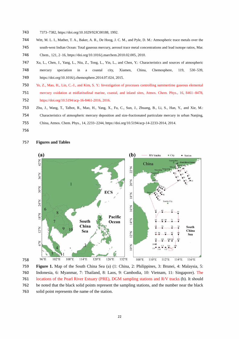
22

7373–7382, https://doi.org/10.1029/92JC00188, 1992. 743

Witt, M. L. I., Mather, T. A., Baker, A. R., De Hoog, J. C. M., and Pyle, D. M.: Atmospheric trace metals over the 744

south-west Indian Ocean: Total gaseous mercury, aerosol trace metal concentrations and lead isotope ratios, Mar. 745

Chem., 121, 2–16, https://doi.org/10.1016/j.marchem.2010.02.005, 2010. 746

Xu, L., Chen, J., Yang, L., Niu, Z., Tong, L., Yin, L., and Chen, Y.: Characteristics and sources of atmospheric 747

mercury speciation in a coastal city, Xiamen, China, Chemosphere, 119, 530–539, 748

https://doi.org/10.1016/j.chemosphere.2014.07.024, 2015. 749

Ye, Z., Mao, H., Lin, C.-J., and Kim, S. Y.: Investigation of processes controlling summertime gaseous elemental 750

mercury oxidation at midlatitudinal marine, coastal, and inland sites, Atmos. Chem. Phys., 16, 84618478, 751

https://doi.org/10.5194/acp-16-8461-2016, 2016. 752

Zhu, J., Wang, T., Talbot, R., Mao, H., Yang, X., Fu, C., Sun, J., Zhuang, B., Li, S., Han, Y., and Xie, M.: 753

Characteristics of atmospheric mercury deposition and size-fractionated particulate mercury in urban Nanjing, 754

China, Atmos. Chem. Phys., 14, 22332244, https://doi.org/10.5194/acp-14-2233-2014, 2014. 755

756

Figures and Tables 757

758

Figure 1. Map of the South China Sea (a) (1: China, 2: Philippines, 3: Brunei, 4: Malaysia, 5: 759

Indonesia, 6: Myanmar, 7: Thailand, 8: Laos, 9: Cambodia, 10: Vietnam, 11: Singapore). The 760

locations of the Pearl River Estuary (PRE), DGM sampling stations and R/V tracks (b). It should 761

be noted that the black solid points represent the sampling stations, and the number near the black 762

solid point represents the name of the station. 763

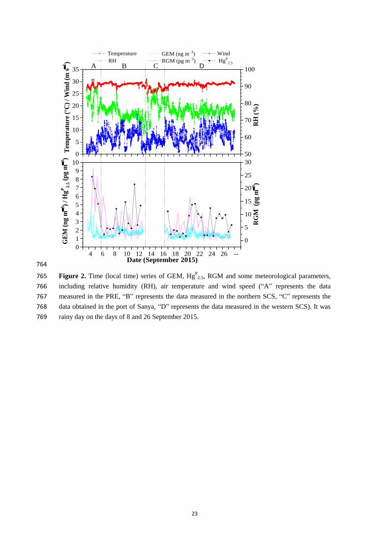
23

0

5

10

15

20

25

30

35

50

60

70

80

90

100

4 6 8 10 12 14 16 18 20 22 24 26 --0

1

2

3

4

5

6

7

8

9

10

0

5

10

15

20

25

30

DBA

RG

M (p

g m

3)

Temperature

Tem

per

atu

re (

°C)

/ W

ind

(m

s

1)

RH

(%

)

C

RH

Wind GEM (ng m3

)

GE

M (

ng

m

3)

/ H

gP

2.5

(p

g m

3)

HgP

2.5

Date (September 2015)

RGM (pg m3

)

764

Figure 2. Time (local time) series of GEM, HgP

2.5, RGM and some meteorological parameters, 765

including relative humidity (RH), air temperature and wind speed (“A” represents the data 766

measured in the PRE, “B” represents the data measured in the northern SCS, “C” represents the 767

data obtained in the port of Sanya, “D” represents the data measured in the western SCS). It was 768

rainy day on the days of 8 and 26 September 2015. 769

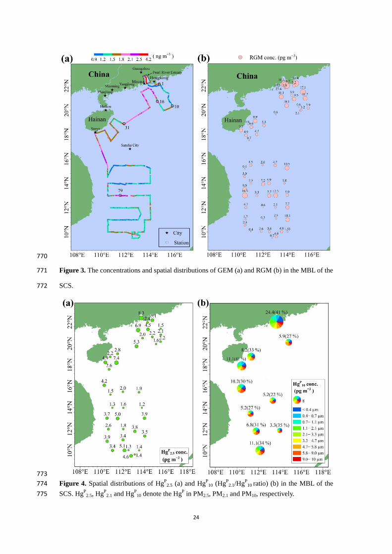
24

770

Figure 3. The concentrations and spatial distributions of GEM (a) and RGM (b) in the MBL of the 771

SCS. 772

773

Figure 4. Spatial distributions of HgP

2.5 (a) and HgP

10 (HgP

2.1/HgP

10 ratio) (b) in the MBL of the 774

SCS. HgP

2.5, HgP

2.1 and HgP

10 denote the HgP in PM2.5, PM2.1 and PM10, respectively. 775

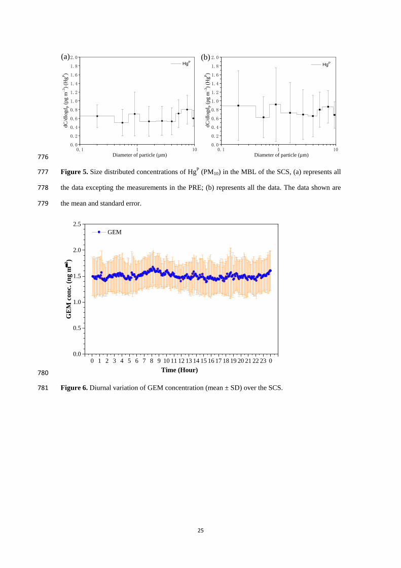
25

0.1 1 100.0

0.2

0.4

0.6

0.8

1.0

1.2

1.4

1.6

1.8

2.0

0.1 1 100.0

0.2

0.4

0.6

0.8

1.0

1.2

1.4

1.6

1.8

2.0

HgP HgP

Diameter of particle (µm)

dC

/dlo

gd

P (

pg

m3)

(Hg

P)

dC

/dlo

gd

P (

pg

m3)

(Hg

P)

Diameter of particle (µm)

(a) (b)

776

Figure 5. Size distributed concentrations of HgP (PM10) in the MBL of the SCS, (a) represents all 777

the data excepting the measurements in the PRE; (b) represents all the data. The data shown are 778

the mean and standard error. 779

0 1 2 3 4 5 6 7 8 9 10 11 12 13 14 15 16 17 18 19 20 21 22 23 00.0

0.5

1.0

1.5

2.0

2.5

GEM

GE

M c

on

c. (

ng m

3)

Time (Hour) 780

Figure 6. Diurnal variation of GEM concentration (mean ± SD) over the SCS. 781

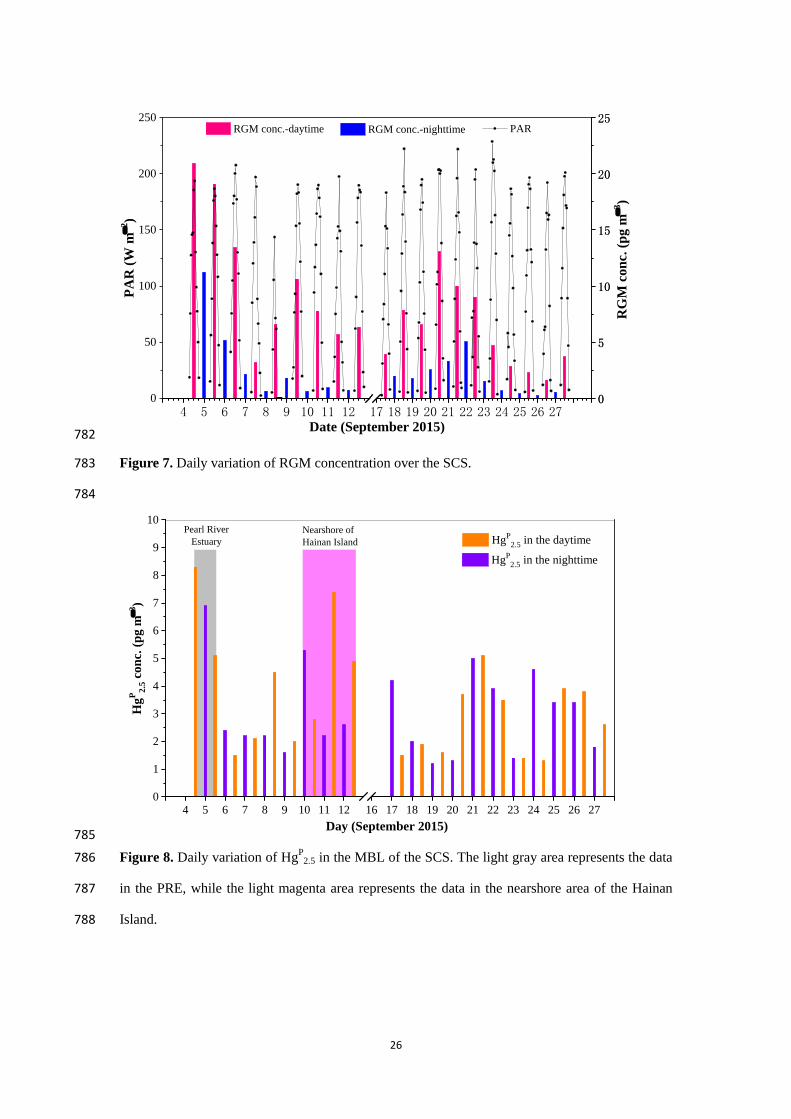
26

0

50

100

150

200

250

4 5 6 7 8 9 10 11 12 17 18 19 20 21 22 23 24 25 26 270

5

10

15

20

25

RGM conc.-nighttime

RG

M c

on

c. (

pg

m

3)

0

5

10

15

20

25

RGM conc.-daytime PARP

AR

(W

m

2)

Date (September 2015) 782

Figure 7. Daily variation of RGM concentration over the SCS. 783

784

4 5 6 7 8 9 10 11 12 16 17 18 19 20 21 22 23 24 25 26 270

1

2

3

4

5

6

7

8

9

10

Hg

P2.5

con

c. (

pg m

3)

HgP

2.5 in the daytime

HgP

2.5 in the nighttime

Pearl River

Estuary

Nearshore of

Hainan Island

Day (September 2015) 785

Figure 8. Daily variation of HgP

2.5 in the MBL of the SCS. The light gray area represents the data 786

in the PRE, while the light magenta area represents the data in the nearshore area of the Hainan 787

Island. 788

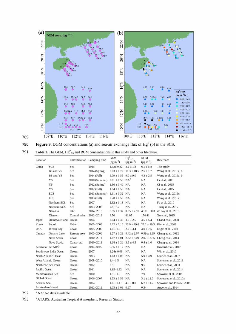
27

789

Figure 9. DGM concentrations (a) and sea-air exchange flux of Hg0 (b) in the SCS. 790

Table 1. The GEM, HgP2.5 and RGM concentrations in this study and other literature. 791

Location Classification Sampling time GEM

(ng m−3

)

HgP

2.5

(pg m−3

)

RGM

(pg m−3

) Reference

China SCS Sea 2015 1.52± 0.32 3.2 ± 1.8 6.1 ± 5.8 This study

BS and YS Sea 2014 (Spring) 2.03 ± 0.72 11.3 ± 18.5 2.5 ± 1.7 Wang et al., 2016a, b

BS and YS Sea 2014 (Fall) 2.09 ± 1.58 9.0 ± 9.0 4.3 ± 2.5 Wang et al., 2016a, b

YS Sea 2010 (Summer) 2.61 ± 0.50 NAa NA Ci et al., 2011

YS Sea 2012 (Spring) 1.86 ± 0.40 NA NA Ci et al., 2015

YS Sea 2012 (Fall) 1.84 ± 0.50 NA NA Ci et al., 2015

ECS Sea 2013 (Summer) 1.61 ± 0.32 NA NA Wang et al., 2016c

ECS Sea 2013 (Fall) 2.20 ± 0.58 NA NA Wang et al., 2016c

Northern SCS Sea 2007 2.62 ± 1.13 NA NA Fu et al., 2010

Northern SCS Sea 2003−2005 2.8 −5.7 NA NA Tseng et al., 2012

Nam Co lake 2014−2015 0.95 ± 0.37 0.85 ± 2.91 49.0 ± 60.3 de Foy et al., 2016

Xiamen Coastal urban 2012−2013 3.50 61.05 174.41 Xu et al., 2015

Japan Okinawa Island Ocean 2004 2.04 ± 0.38 3.0 ± 2.5 4.5 ± 5.4 Chand et al., 2008

Korea Seoul Urban 2005−2006 3.22 ± 2.10 23.9 ± 19.6 27.2 ± 19.3 Kim et al., 2009

USA Weeks Bay Coast 2005−2006 1.6 ± 0.3 2.7 ± 3.4 4.0 ± 7.5 Engle et al., 2008

Canada Ontario Lake Remote area 2005−2006 1.57 ± 0.22 4.42 ± 3.67 0.99 ± 1.89 Cheng et al., 2012

Nova Scotia Coast 2010−2011 1.67 ± 1.01 2.32 ± 3.09 2.07 ± 3.35 Cheng et al., 2013

Nova Scotia Coast-rural 2010−2011 1.38 ± 0.20 3.5 ± 4.5 0.4 ± 1.0 Cheng et al., 2014

Australia ATARSb Coast 2014-2015 0.95 ± 0.12 NA NA Howard et al., 2017

South-west India Ocean Ocean 2007 1.24± 0.06 NA NA Witt et al., 2010

North Atlantic Ocean Ocean 2003 1.63 ± 0.08 NA 5.9 ± 4.9 Laurier et al., 2007

West Atlantic Ocean Ocean 2008−2010 1.41.5 NA NA Soerensen et al., 2013

North Pacific Ocean Ocean 2002 2.5 NA 9.5 Laurier et al., 2003

Pacific Ocean Ocean 2011 1.151.32 NA NA Soerensen et al., 2014

Mediterranean Sea Sea 2000 1.9 ± 1.0 NA 7.9 Sprovieri et al., 2003

Global Ocean

Ocean

Ocean 2006−2007 1.53 ± 0.58 NA 3.1 ± 11.0 Soerensen et al., 2010a

Adriatic Sea Ocean 2004 1.6 ± 0.4 4.5 ± 8.0 6.7 ± 11.7 Sprovieri and Pirrone, 2008

Amsterdam Island

terdam Island

Ocean 2012−2013 1.03 ± 0.08 0.67 0.34 Angot et al., 2014

a NA: No data available. 792 b ATARS: Australian Tropical Atmospheric Research Station. 793

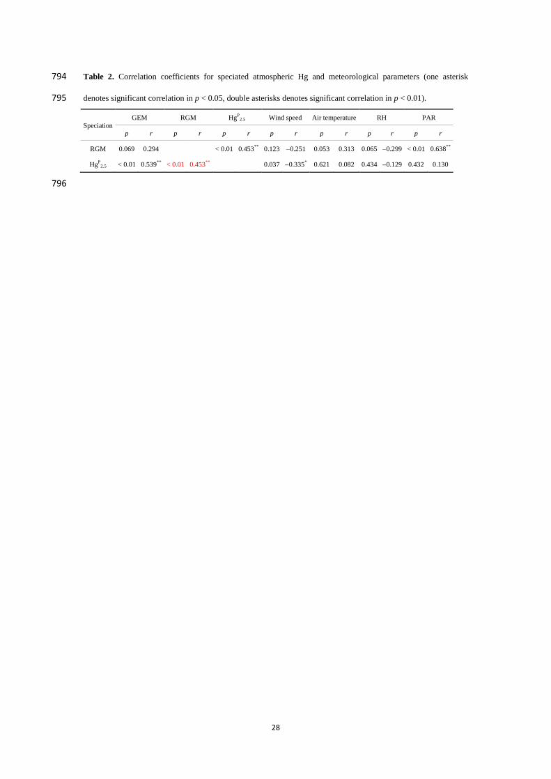
28

Table 2. Correlation coefficients for speciated atmospheric Hg and meteorological parameters (one asterisk 794

denotes significant correlation in p < 0.05, double asterisks denotes significant correlation in p < 0.01). 795

Speciation GEM RGM Hg

P2.5 Wind speed Air temperature RH PAR

p r p r p r p r p r p r p r

RGM 0.069 0.294 < 0.01 0.453**

0.123 0.251 0.053 0.313 0.065 0.299 < 0.01 0.638**

HgP

2.5 < 0.01 0.539**

< 0.01 0.453**

0.037 0.335* 0.621 0.082 0.434 0.129 0.432 0.130

796

1

Supplement of 1

Speciated atmospheric mercury and sea-air exchange of 2

gaseous mercury in the South China Sea 3

Chunjie Wang1, Zhangwei Wang

1, Fan Hui

2, Xiaoshan Zhang

1 4

1 Research Center for Eco-Environmental Sciences, Chinese Academy of Sciences, 18 Shuangqing Road, Beijing, 5

China 6

2 China University of Petroleum (Beijing), 18 Fuxue Road, Beijing, China 7

Correspondence to: Xiaoshan Zhang (zhangxsh@rcees.ac.cn) 8

9

10

11

12

13

14

15

16

17

18

19

20

21

22

23

24

25

26

27

28

29

30

31

32

33

34

35

36

37

38

39

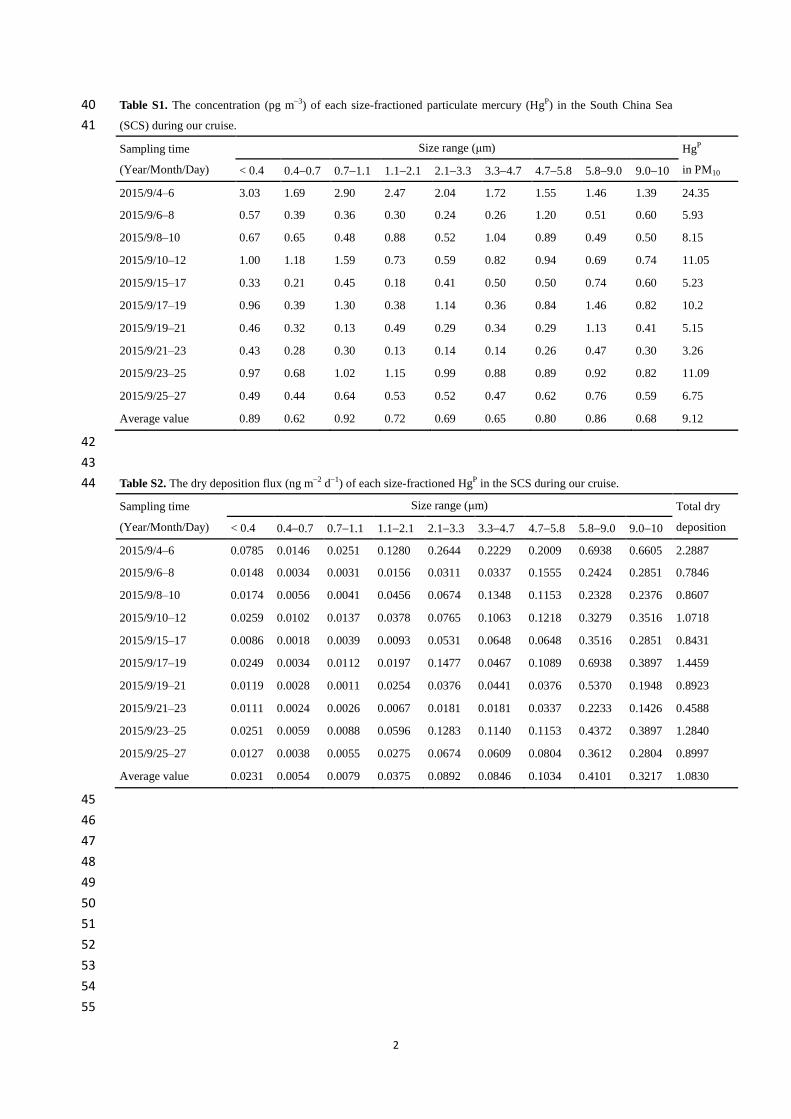
2

Table S1. The concentration (pg m3) of each size-fractioned particulate mercury (HgP) in the South China Sea 40

(SCS) during our cruise. 41

Sampling time

(Year/Month/Day)

Size range (μm) HgP

in PM10 < 0.4 0.40.7 0.71.1 1.12.1 2.13.3 3.34.7 4.75.8 5.89.0 9.010

2015/9/4–6 3.03 1.69 2.90 2.47 2.04 1.72 1.55 1.46 1.39 24.35

2015/9/6–8 0.57 0.39 0.36 0.30 0.24 0.26 1.20 0.51 0.60 5.93

2015/9/8–10 0.67 0.65 0.48 0.88 0.52 1.04 0.89 0.49 0.50 8.15

2015/9/10–12 1.00 1.18 1.59 0.73 0.59 0.82 0.94 0.69 0.74 11.05

2015/9/15–17 0.33 0.21 0.45 0.18 0.41 0.50 0.50 0.74 0.60 5.23

2015/9/17–19 0.96 0.39 1.30 0.38 1.14 0.36 0.84 1.46 0.82 10.2

2015/9/19–21 0.46 0.32 0.13 0.49 0.29 0.34 0.29 1.13 0.41 5.15

2015/9/21–23 0.43 0.28 0.30 0.13 0.14 0.14 0.26 0.47 0.30 3.26

2015/9/23–25 0.97 0.68 1.02 1.15 0.99 0.88 0.89 0.92 0.82 11.09

2015/9/25–27 0.49 0.44 0.64 0.53 0.52 0.47 0.62 0.76 0.59 6.75

Average value 0.89 0.62 0.92 0.72 0.69 0.65 0.80 0.86 0.68 9.12

42

43

Table S2. The dry deposition flux (ng m2 d1) of each size-fractioned HgP in the SCS during our cruise. 44

Sampling time

(Year/Month/Day)

Size range (μm) Total dry

deposition < 0.4 0.40.7 0.71.1 1.12.1 2.13.3 3.34.7 4.75.8 5.89.0 9.010

2015/9/4–6 0.0785 0.0146 0.0251 0.1280 0.2644 0.2229 0.2009 0.6938 0.6605 2.2887

2015/9/6–8 0.0148 0.0034 0.0031 0.0156 0.0311 0.0337 0.1555 0.2424 0.2851 0.7846

2015/9/8–10 0.0174 0.0056 0.0041 0.0456 0.0674 0.1348 0.1153 0.2328 0.2376 0.8607

2015/9/10–12 0.0259 0.0102 0.0137 0.0378 0.0765 0.1063 0.1218 0.3279 0.3516 1.0718

2015/9/15–17 0.0086 0.0018 0.0039 0.0093 0.0531 0.0648 0.0648 0.3516 0.2851 0.8431

2015/9/17–19 0.0249 0.0034 0.0112 0.0197 0.1477 0.0467 0.1089 0.6938 0.3897 1.4459

2015/9/19–21 0.0119 0.0028 0.0011 0.0254 0.0376 0.0441 0.0376 0.5370 0.1948 0.8923

2015/9/21–23 0.0111 0.0024 0.0026 0.0067 0.0181 0.0181 0.0337 0.2233 0.1426 0.4588

2015/9/23–25 0.0251 0.0059 0.0088 0.0596 0.1283 0.1140 0.1153 0.4372 0.3897 1.2840

2015/9/25–27 0.0127 0.0038 0.0055 0.0275 0.0674 0.0609 0.0804 0.3612 0.2804 0.8997

Average value 0.0231 0.0054 0.0079 0.0375 0.0892 0.0846 0.1034 0.4101 0.3217 1.0830

45

46

47

48

49

50

51

52

53

54

55

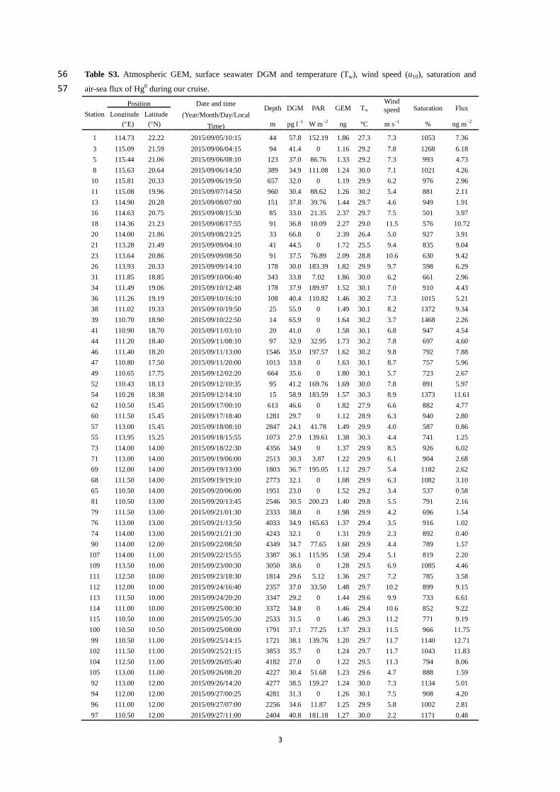
3

Table S3. Atmospheric GEM, surface seawater DGM and temperature (Tw), wind speed (u10), saturation and 56

air-sea flux of Hg0 during our cruise. 57

Station

Position Date and time

(Year/Month/Day/Local

Time)

Depth DGM PAR GEM Tw Wind

speed

u10

Saturation Flux Longitude Latitude

(E) (N) m pg l−1

W m−2

ng

m−3

°C m s−1

% ng m−2

h−1

1 114.73 22.22 2015/09/05/10:15 44 57.8 152.19 1.86 27.3 7.3 1053 7.36

3 115.09 21.59 2015/09/06/04:15 94 41.4 0 1.16 29.2 7.8 1268 6.18

5 115.44 21.06 2015/09/06/08:10 123 37.0 86.76 1.33 29.2 7.3 993 4.73

8 115.63 20.64 2015/09/06/14:50 389 34.9 111.08 1.24 30.0 7.1 1021 4.26

10 115.81 20.33 2015/09/06/19:50 657 32.0 0 1.19 29.9 6.2 976 2.96

11 115.08 19.96 2015/09/07/14:50 960 30.4 88.62 1.26 30.2 5.4 881 2.11

13 114.90 20.28 2015/09/08/07:00 151 37.8 39.76 1.44 29.7 4.6 949 1.91

16 114.63 20.75 2015/09/08/15:30 85 33.0 21.35 2.37 29.7 7.5 501 3.97

18 114.36 21.23 2015/09/08/17:55 91 36.8 10.09 2.27 29.0 11.5 576 10.72

20 114.00 21.86 2015/09/08/23:25 33 66.8 0 2.39 26.4 5.0 927 3.91

21 113.28 21.49 2015/09/09/04:10 41 44.5 0 1.72 25.5 9.4 835 9.04

23 113.64 20.86 2015/09/09/08:50 91 37.5 76.89 2.09 28.8 10.6 630 9.42

26 113.93 20.33 2015/09/09/14:10 178 30.0 183.39 1.82 29.9 9.7 598 6.29

31 111.85 18.85 2015/09/10/06:40 343 33.8 7.02 1.86 30.0 6.2 661 2.96

34 111.49 19.06 2015/09/10/12:48 178 37.9 189.97 1.52 30.1 7.0 910 4.43

36 111.26 19.19 2015/09/10/16:10 108 40.4 110.82 1.46 30.2 7.3 1015 5.21

38 111.02 19.33 2015/09/10/19:50 25 55.9 0 1.49 30.1 8.2 1372 9.34

39 110.70 18.90 2015/09/10/22:50 14 65.9 0 1.64 30.2 3.7 1468 2.26

41 110.90 18.70 2015/09/11/03:10 20 41.0 0 1.58 30.1 6.8 947 4.54

44 111.20 18.40 2015/09/11/08:10 97 32.9 32.95 1.73 30.2 7.8 697 4.60

46 111.40 18.20 2015/09/11/13:00 1546 35.0 197.57 1.62 30.2 9.8 792 7.88

47 110.80 17.50 2015/09/11/20:00 1013 33.8 0 1.63 30.1 8.7 757 5.96

49 110.65 17.75 2015/09/12/02:20 664 35.6 0 1.80 30.1 5.7 723 2.67

52 110.43 18.13 2015/09/12/10:35 95 41.2 169.76 1.69 30.0 7.8 891 5.97

54 110.28 18.38 2015/09/12/14:10 15 58.9 183.59 1.57 30.3 8.9 1373 11.61

62 110.50 15.45 2015/09/17/00:10 613 46.6 0 1.82 27.9 6.6 882 4.77

60 111.50 15.45 2015/09/17/18:40 1281 29.7 0 1.12 28.9 6.3 940 2.80

57 113.00 15.45 2015/09/18/08:10 2847 24.1 41.78 1.49 29.9 4.0 587 0.86

55 113.95 15.25 2015/09/18/15:55 1073 27.9 139.61 1.38 30.3 4.4 741 1.25

73 114.00 14.00 2015/09/18/22:30 4356 34.9 0 1.37 29.9 8.5 926 6.02

71 113.00 14.00 2015/09/19/06:00 2513 30.3 3.87 1.22 29.9 6.1 904 2.68

69 112.00 14.00 2015/09/19/13:00 1803 36.7 195.05 1.12 29.7 5.4 1182 2.62

68 111.50 14.00 2015/09/19/19:10 2773 32.1 0 1.08 29.9 6.3 1082 3.10

65 110.50 14.00 2015/09/20/06:00 1951 23.0 0 1.52 29.2 3.4 537 0.58

81 110.50 13.00 2015/09/20/13:45 2546 30.5 200.23 1.40 29.8 5.5 791 2.16

79 111.50 13.00 2015/09/21/01:30 2333 38.0 0 1.98 29.9 4.2 696 1.54

76 113.00 13.00 2015/09/21/13:50 4033 34.9 165.63 1.37 29.4 3.5 916 1.02

74 114.00 13.00 2015/09/21/21:30 4243 32.1 0 1.31 29.9 2.3 892 0.40

90 114.00 12.00 2015/09/22/08:50 4349 34.7 77.65 1.60 29.9 4.4 789 1.57

107 114.00 11.00 2015/09/22/15:55 3387 36.1 115.95 1.58 29.4 5.1 819 2.20

109 113.50 10.00 2015/09/23/00:30 3050 38.6 0 1.28 29.5 6.9 1085 4.46

111 112.50 10.00 2015/09/23/18:30 1814 29.6 5.12 1.36 29.7 7.2 785 3.58

112 112.00 10.00 2015/09/24/16:40 2357 37.0 33.50 1.48 29.7 10.2 899 9.15

113 111.50 10.00 2015/09/24/20:20 3347 29.2 0 1.44 29.6 9.9 733 6.61

114 111.00 10.00 2015/09/25/00:30 3372 34.8 0 1.46 29.4 10.6 852 9.22

115 110.50 10.00 2015/09/25/05:30 2533 31.5 0 1.46 29.3 11.2 771 9.19

100 110.50 10.50 2015/09/25/08:00 1791 37.1 77.25 1.37 29.3 11.5 966 11.75

99 110.50 11.00 2015/09/25/14:15 1721 38.1 139.76 1.20 29.7 11.7 1140 12.71

102 111.50 11.00 2015/09/25/21:15 3853 35.7 0 1.24 29.7 11.7 1043 11.83

104 112.50 11.00 2015/09/26/05:40 4182 27.0 0 1.22 29.5 11.3 794 8.06

105 113.00 11.00 2015/09/26/08:20 4227 30.4 51.68 1.23 29.6 4.7 888 1.59

92 113.00 12.00 2015/09/26/14:20 4277 38.5 159.27 1.24 30.0 7.3 1134 5.01

94 112.00 12.00 2015/09/27/00:25 4281 31.3 0 1.26 30.1 7.5 908 4.20

96 111.00 12.00 2015/09/27/07:00 2256 34.6 11.87 1.25 29.9 5.8 1002 2.81

97 110.50 12.00 2015/09/27/11:00 2404 40.8 181.18 1.27 30.0 2.2 1171 0.48

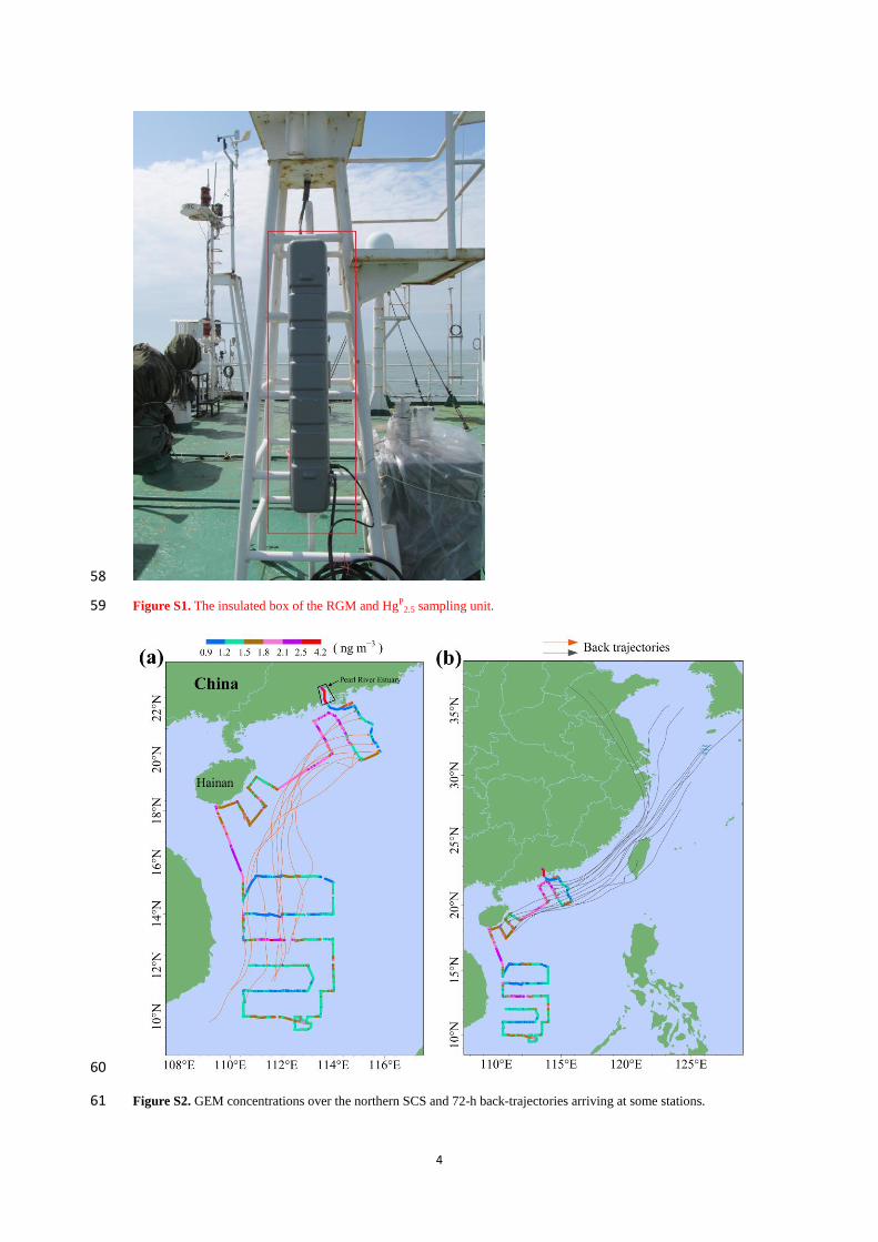
4

58

Figure S1. The insulated box of the RGM and HgP2.5 sampling unit. 59

60

Figure S2. GEM concentrations over the northern SCS and 72-h back-trajectories arriving at some stations. 61

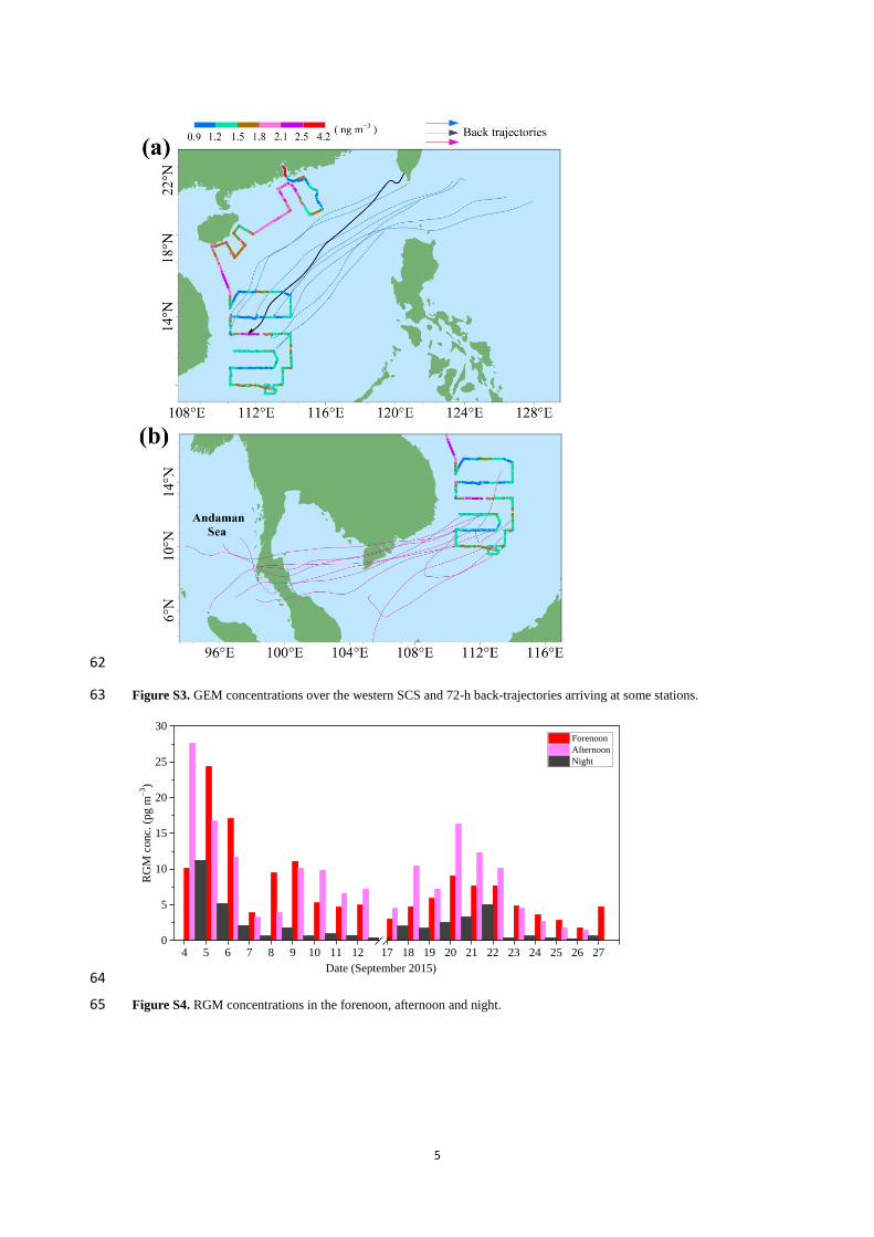
5

62

Figure S3. GEM concentrations over the western SCS and 72-h back-trajectories arriving at some stations. 63

0

5

10

15

20

25

30

RG

M c

onc.

(pg m

3)

Forenoon

Afternoon

Night

4 5 6 7 8 9 10 11 12 17 18 19 20 21 22 23 24 25 26 27

Date (September 2015) 64

Figure S4. RGM concentrations in the forenoon, afternoon and night. 65