Embed Size (px)
Citation preview
19
Retroactive Packet Sampling for Traffic Receipts
PAVLOS NIKOLOPOULOS∗, CHRISTOS PAPPAS+, KATERINA ARGYRAKI∗,ADRIAN PERRIG+, ∗EPFL, Switzerland, +ETHZ, Switzerland
Is it possible to design a packet-sampling algorithm that prevents the network node that performs the sampling
from treating the sampled packets preferentially? We study this problem in the context of designing a “network
transparency” system. In this system, networks emit receipts for a small sample of the packets they observe,
and a monitor collects these receipts to estimate each network’s loss and delay performance. Sampling is a
good building block for this system, because it enables a solution that is flexible and combines low resource cost
with quantifiable accuracy. The challenge is cheating resistance: when a network’s performance is assessed
based on the conditions experienced by a small traffic sample, the network has a strong incentive to treat
the sampled packets better than the rest. We contribute a sampling algorithm that is provably robust to
such prioritization attacks, enables network performance estimation with quantifiable accuracy, and requires
minimal resources. We confirm our analysis using real traffic traces.
CCS Concepts: • Networks→ Data path algorithms; Network measurement;
ACM Reference Format:Pavlos Nikolopoulos
∗, Christos Pappas
+, Katerina Argyraki
∗, Adrian Perrig
+. 2019. Retroactive Packet Sam-
pling for Traffic Receipts. Proc. ACM Meas. Anal. Comput. Syst. 3, 1, Article 19 (March 2019), 39 pages.
https://doi.org/10.1145/3311090
1 INTRODUCTIONWe study the following problem: is it possible to design a packet-sampling algorithm that prevents
the network node that performs the sampling from treating the sampled packets preferentially?
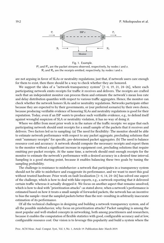
For instance, consider the Internet Service Provider (ISP) shown in Fig. 1 and suppose that it emits
“traffic receipts” (essentially digests and timestamps) for a small sample of the packets that enter and
exit its network; a monitor collects these receipts and uses them to periodically estimate the ISP’s
loss rate and delay distribution. Since the ISP’s performance is estimated based on how it treats the
sampled packets, the ISP has an incentive to cheat: treat the sampled packets better than the rest
(e.g., forward them through a lower-loss, lower-delay intra-domain path) in order to exaggerate its
performance. Is it possible to design a packet-sampling algorithm that prevents such behavior?
Our motivation for studying this problem is the need for more network transparency. In the
current Internet, when packets get lost or delayed, there is typically no information about where
the problem occurred, hence no information about who is responsible. This results in service
level agreements (SLAs) and neutrality regulations that cannot be enforced: First, ISPs guarantee
that their network will honor a minimum delivery rate (equivalently, a maximum loss rate) and
a maximum latency [8, 9, 23], even though there exists no systematic way to estimate their loss
rate or delay distribution. Second, governments require that ISPs not (de)prioritize certain traffic
classes [7, 10, 20], even though there exists no systematic way to detect traffic (de)prioritization. We
Author’s address: Pavlos Nikolopoulos∗, Christos Pappas
+, Katerina Argyraki
∗,
Adrian Perrig+∗EPFL, Switzerland,
+ETHZ, Switzerland.
Permission to make digital or hard copies of all or part of this work for personal or classroom use is granted without fee
provided that copies are not made or distributed for profit or commercial advantage and that copies bear this notice and
the full citation on the first page. Copyrights for components of this work owned by others than ACM must be honored.
Abstracting with credit is permitted. To copy otherwise, or republish, to post on servers or to redistribute to lists, requires
prior specific permission and/or a fee. Request permissions from [email protected].
© 2019 Association for Computing Machinery.
2476-1249/2019/3-ART19 $15.00
https://doi.org/10.1145/3311090
Proc. ACM Meas. Anal. Comput. Syst., Vol. 3, No. 1, Article 19. Publication date: March 2019.
19:2 P. Nikolopoulos et al.
i o
Pi PoISP x
Monitor
Ri Ro
Fig. 1. Example.Pi and Po are the packet streams observed, respectively, by nodes i and o.Ri and Ro are the receipts emitted, respectively, by nodes i and o.
are not arguing in favor of SLAs or neutrality regulations; just that, if network users care enough
for them to exist, then there should be a way to check whether they are honored.
We support the idea of a “network-transparency system” [1–4, 19, 21, 24–26], where each
participating network emits receipts for traffic it receives and delivers. The receipts are crafted
such that an independent monitor can process them and estimate the network’s mean loss rate
and delay distribution quantiles with respect to various traffic aggregates. Hence, the monitor can
check whether the network honors SLAs and/or neutrality regulations. Networks participate either
because they are expected to by their governments, or (our preferred scenario) by their own choice,
because producing verifiable evidence of honoring SLAs and neutrality regulations is good for their
reputation. Today, even if an ISP wants to produce such verifiable evidence, e.g., to defend itself
against wrongful suspicion of SLA or neutrality violation, it has no way of doing it.
Where we differ from most prior work is in the nature of the traffic receipts: we argue that each
participating network should emit receipts for a small sample of the packets that it receives and
delivers. Two factors led us to sampling: (a) The need for flexibility: The monitor should be able
to estimate network performance with respect to any packet aggregate, precluding solutions that
emit “summary receipts” for specific, pre-determined packet aggregates. (b) The need to balance
resource cost and accuracy: A network should compute the necessary receipts and export them
to the monitor without a significant increase in equipment cost, precluding solutions that require
emitting per-packet receipts. At the same time, a network should emit enough receipts for the
monitor to estimate the network’s performance with a desired accuracy in a desired time interval.
Sampling is a good starting point, because it enables balancing these two goals by tuning the
sampling probability.
The challenge is resistance to misbehavior: a network that participates in a transparency system
should not be able to misbehave and exaggerate its performance, and we want to meet this goal
without trusted hardware. Prior work on fault localization [1–4, 14, 24–26] has solved one aspect
of the challenge, which is how to deal with fake reports, e.g., a network reporting that it delivered
certain traffic whereas it actually dropped it. We focus on another aspect that remains unsolved,
which is how to deal with “prioritization attacks”: as stated above, when a network’s performance is
estimated based on how it treats a small sample of forwarded packets, the network has an incentive
to bias the sample—treat the sampled packets better than the rest—resulting in arbitrarily inaccurate
estimation of its performance.
Of all the technical challenges in designing and building a network transparency system, and of
all the possible misbehavior, why focus on prioritization attacks? Packet sampling is among the
most popular and well-studied concepts in networking, both among practitioners and researchers,
because it enables the computation of flexible statistics with good, configurable accuracy and at low,
configurable resource cost. Our vision is to leverage this popularity and build a system where the
Proc. ACM Meas. Anal. Comput. Syst., Vol. 3, No. 1, Article 19. Publication date: March 2019.
Retroactive Packet Sampling for Traffic Receipts 19:3
data-plane of each network emits information on a small, configurable sample of observed traffic,
and this information is used both for the network’s internal management and troubleshooting (as
already happens today) and (after proper filtering) for network transparency. For this to work, the
fundamental challenge is ensuring that the sample is representative without assuming that the
data-plane, which chooses and handles the sample, is trusted; this is what we set out to solve.
We build on the idea of sampling with delayed disclosure [3]: when a network node observes
a packet p, it cannot immediately determine whether it should sample p or not, because that
information is disclosed by subsequent traffic; by the time disclosure happens, the node has
normally forwarded p, hence cannot treat it according to its sampling fate. We call the sampling
algorithm proposed in [3] “basic delayed disclosure.”
Basic delayed disclosure is promising, however, an analysis of the algorithm reveals flaws: First,
vulnerability to subtle prioritization attacks (§7.4), where a misbehaving network buffers packets
long enough to learn their sampling fate with a non-trivial probability, yet short enough not
to introduce significant buffering delays; we show that such an attack enables a misbehaving
network to claim significantly less loss and delay (as much as 41% in our experiments) than it
actually introduces. Second, in many realistic scenarios, achieving good accuracy in a timely manner
requires many tens of MBs of data-path memory per 10Gbps of forwarding capacity (§6); at this
cost, we might as well use a completely different approach from sampling, e.g., maintain explicit
per-flow loss and delay information on the data-path, which is not vulnerable to prioritization
attacks in the first place.
Our contribution is a sampling algorithm (§3) that corrects these flaws: First, it is robust to
prioritization attacks (§4). Second, it uses the minimum amount of data-path memory necessary for
achieving a desired accuracy in a desired time interval (§5). As a result, it achieves good accuracy
in a timely manner, while requiring a modest amount of resources, affordable by modern networks;
for instance, in the same scenario where basic delayed disclosure requires many tens of MBs of
data-path memory per 10Gbps of forwarding capacity, our algorithm requires only a couple of
MB—an order of magnitude less (§6). To achieve these properties, we enhance delayed disclosure
with carefully regulated “quiet periods,” during which no sampling may occur, and with a new
disclosure process, which is continuously adapted to the observed traffic. These two techniques
allow us to control the pace of disclosure, such that we emit no more receipts than necessary and
make prioritization attacks ineffective: by the time a misbehaving network has learned the sampling
fate of a packet (with a non-trivial probability), it has buffered—hence delayed—the packet for so
long that it cannot benefit from prioritization any more. Our experimental evaluation confirms our
analysis using real traffic traces (§7).
2 SETUPIn this section, we state our terminology (§2.1), the problem we solve (2.2), the starting point for
our solution (§2.3), our trust model (§2.4), and our assumptions and limitations (§2.5).
2.1 TerminologyA “domain” is a contiguous network area managed by a single administrative entity, e.g., an ISP, an
Autonomous System (AS), an Internet eXchange Point (IXP), an enterprise or campus network, the
data-center network of a content provider.
Each domain that participates in our system deploys a special “node” at each point where it
exchanges traffic with another domain. Each node runs an algorithm (from now on referred to as
“the algorithm”) that takes as input a set of configuration parameters and the sequence of packets
Proc. ACM Meas. Anal. Comput. Syst., Vol. 3, No. 1, Article 19. Publication date: March 2019.

19:4 P. Nikolopoulos et al.
arriving at the node, and outputs a set of “receipts.” A node is always collocated with a border
router and can be implemented on the linecards that handle the packets as they enter and exit the
domain.
The “monitor” is an entity that collects the receipts emitted by the participating domains and uses
them to estimate domain performance. It can be owned and managed by one authority, e.g., like
the root DNS servers, or it can be a decentralized system, owned and managed by the participating
domains themselves.
We define two kinds of traffic units: “flows” and “aggregates.” A “flow” is the set of packets
observed by a node that have the same source and destination IP prefix. An “aggregate” is a set of
packets with some common observable characteristic, e.g., the set of packets from a given source to
a given destination domain, or all BitTorrent packets from a given source domain; so, an aggregate
may be a flow’s subset or consist of one or multiple flows. An aggregate’s “source node” is the first
node that observes all traffic from that aggregate. Nodes can classify packets per flow but are not
aware of aggregates. The monitor, on the other hand, estimates domain performance with respect
to aggregates that it defines as needed (examples in §7.2).
In our context, the monitor is trusted, while a node (and the domain that owns the node) may
“misbehave,” i.e., try to cause the monitor to produce incorrect estimates that exaggerate the
domain’s performance.
2.2 GoalsWe set three goals:
1) Given an aggregate A, the monitor should be able to estimate each participating domain’s
mean loss rate and delay distribution quantiles with respect toAwith a given target (γ , ϵ)-accuracy,where γ is the probability that the relative estimation error is below ϵ . This is a standard accuracy
metric for loss estimates and was recently defined for delay estimates as well [5, 22].
2) A domain should be able to deploy and run the algorithm on a node without increasing the
node’s data-to-control-path bandwidth and data-path memory by more than a few percentage
points.
3) A misbehaving domain should not be able to significantly exaggerate its performance by
manipulating either the receipts emitted by its nodes or their forwarding process.
2.3 Starting Point: SamplingEach node emits a receipt for a small sample of packets, drawn from all the packets it observes.
Each receipt carries: a digest that uniquely identifies the packet with high probability; a timestampthat specifies when the packet was observed at the node; and a flow ID that specifies the packet’s
source and destination IP prefix.
Each node draws the sample it reports on from all the packets it observes. If, instead, we reactivelyconfigured the nodes to emit receipts for a specific aggregate of interest A, e.g., in reaction to user
suspicions that A is being throttled, then a dishonest domain could change how it treats A the
moment it starts reporting on it.
2.4 Attack ModelWe classify misbehavior into “fake receipts,” where a domain emits incorrect receipts that exaggerate
its performance; and “prioritization,” where a domain emits correct receipts but manipulates its
forwarding process in order to exaggerate its performance. We briefly discuss the former here and
focus on the latter in the rest of the paper.
Proc. ACM Meas. Anal. Comput. Syst., Vol. 3, No. 1, Article 19. Publication date: March 2019.
Retroactive Packet Sampling for Traffic Receipts 19:5
In a fake-receipt attack, a node emits a set of receipts that is different from the one produced by
the algorithm. For example, it may suppress a receipt (pretend that it never received a packet that
it actually did receive and dropped), emit a superfluous receipt (pretend that it delivered a packet
that it actually dropped), or modify receipt timestamps (pretend that it received a packet later, or
delivered a packet earlier than it actually did).
We now outline how these attacks can be addressed based on ideas from prior work [1–4, 14,
24–26]. One way to prevent fake-receipt attacks is through incentives: (1) If domain x ’s receiptmanipulation does not improve x ’s estimated performance, then x has no incentive to launch such
an attack. (2) If x ’s receipt manipulation necessarily and visibly implicates x ’s neighbor y, thenx has an incentive to not launch such an attack, as that would affect its business relationship to
y. Such incentives can be created with consistent sampling [27]: Each node hashes part of the
non-mutable contents of each observed packet and samples the packet if the outcome falls within a
pre-determined range [13, 18]. A hash function with strong randomization properties results in
uniform sampling, where the sampling probability is determined by the range of the hash function.
As a result, a packet is either sampled by all the nodes that observe it or by none of them.
Definition 2.1. Consider a packet p from a flow F that traverses a node i and then another node
o. We say that nodes i and o “sample p consistently” if the conditional probability that o samples pgiven that o observes p and i samples p is 1.
With consistent sampling, a fake receipt shifts the blame for a lost or delayed packet to an
inter-domain link; since an inter-domain link is shared responsibility with a neighbor, a fake receipt
does not exonerate the culprit, while it necessarily and visibly implicates the culprit’s neighbor.
For example, suppose domain y delivers packet p to domain x , which drops it; both y and x sample
p, but x suppresses the receipt produced for p at its entry point, i.e., pretends that it never received
p. Since y produces a receipt for p but x does not, the monitor concludes that p was dropped on
the inter-domain link between y and x , and it attributes the loss to both x and y. Hence, x is not
exonerated, and it also implicatesy. Moreover,y can monitor its inter-domain link with x , determine
that it is not faulty/congested (hence cannot have dropped p), and detect x ’s misbehavior.
In a prioritization attack, a node emits the set of receipts that is produced by the algorithm but
manipulates its forwarding process: it treats some or all of the sampled packets preferentially, e.g.,
by assigning them to higher-priority/lower-priority queues or routing them through better/worse
paths. Prior work has considered these attacks [3] but not solved them (§7.4).
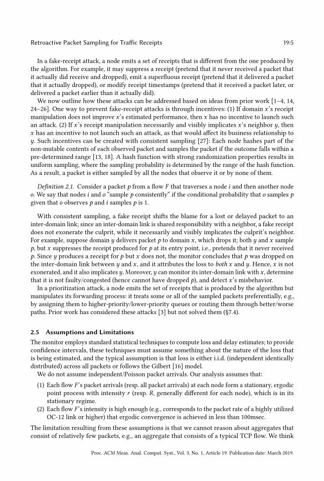
2.5 Assumptions and LimitationsThe monitor employs standard statistical techniques to compute loss and delay estimates; to provide
confidence intervals, these techniques must assume something about the nature of the loss that
is being estimated, and the typical assumption is that loss is either i.i.d. (independent identically
distributed) across all packets or follows the Gilbert [16] model.
We do not assume independent/Poisson packet arrivals. Our analysis assumes that:
(1) Each flow F ’s packet arrivals (resp. all packet arrivals) at each node form a stationary, ergodic
point process with intensity r (resp. R, generally different for each node), which is in its
stationary regime.
(2) Each flow F ’s intensity is high enough (e.g., corresponds to the packet rate of a highly utilized
OC-12 link or higher) that ergodic convergence is achieved in less than 100msec.
The limitation resulting from these assumptions is that we cannot reason about aggregates that
consist of relatively few packets, e.g., an aggregate that consists of a typical TCP flow. We think
Proc. ACM Meas. Anal. Comput. Syst., Vol. 3, No. 1, Article 19. Publication date: March 2019.
19:6 P. Nikolopoulos et al.
Symbolsp A packet
d A disclosure packet
F A flow
Workload characteristicsr Intensity (in packets/sec) of a flow’s packet arrivals at a node
R Intensity (in packets/sec) of all packet arrivals at a node
Algorithm parametersβ The size of the receipt buffer (different at each node)
κ The duration of the quiet period
µ Jitter margin: subset of the quiet period during which packets are sampled
δrDisclosure rate: probability that a node picks a packet from a flow
with intensity r as a disclosure packet
σSelection rate: conditional probability that a node samples a packet
given that the packet does not suffer early or late disclosure at the node
Other configuration parameters(γ , ϵ) Target accuracy (confidence level and error) for the monitor’s estimates
T Target time interval in which the target accuracy should be achieved
Nγ ,ϵ Minimum number of samples needed to achieve the target accuracy
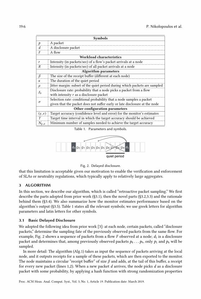
Table 1. Parameters and symbols.
quiet period
!" p9p8p7p6p5p4p3p2p1p0 !#
Fig. 2. Delayed disclosure.
that this limitation is acceptable given our motivation to enable the verification and enforcement
of SLAs or neutrality regulations, which typically apply to relatively large aggregates.
3 ALGORITHMIn this section, we describe our algorithm, which is called “retroactive packet sampling.” We first
describe the parts adopted from prior work (§3.1), then the novel parts (§3.2,3.3) and the rationale
behind them (§3.4). We also summarize how the monitor estimates performance based on the
algorithm’s output (§3.5). Table 1 states all the relevant symbols; we use greek letters for algorithm
parameters and latin letters for other symbols.
3.1 Basic Delayed DisclosureWe adopted the following idea from prior work [3]: at each node, certain packets, called “disclosure
packets,” determine the sampling fate of the previously observed packets from the same flow. For
example, Fig. 2 shows a sequence of packets from a flow F observed at a node; d1 is a disclosurepacket and determines that, among previously observed packets p0 . . . p9, only p1 and p4 will besampled.
In more detail: The algorithm (Alg.1) takes as input the sequence of packets arriving at the local
node, and it outputs receipts for a sample of these packets, which are then exported to the monitor.
The node maintains a circular “receipt buffer” of size β and adds, at the tail of this buffer, a receipt
for every new packet (lines 1,2). When a new packet d arrives, the node picks d as a disclosure
packet with some probability, by applying a hash function with strong randomization properties
Proc. ACM Meas. Anal. Comput. Syst., Vol. 3, No. 1, Article 19. Publication date: March 2019.
Retroactive Packet Sampling for Traffic Receipts 19:7
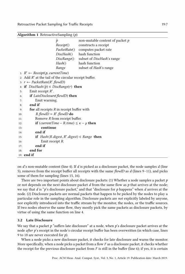
Algorithm 1 RetroactiveSampling (p)
p̂ non-mutable content of packet pReceipt() constructs a receipt
PacketRate() computes packet rate
DiscHash() hash function
DiscRange() subset of DiscHash’s rangeHash() hash function
Range subset of Hash’s range1: R′← Receipt(p, currentTime)2: Add R′ at the tail of the circular receipt buffer.3: r ← PacketRate(R′.flowID)4: if DiscHash (p̂) ∈ DiscRange(r ) then5: Emit receipt R′.6: if LateDisclosure(flowID) then7: Emit warning.
8: end if9: for all receipts R in receipt buffer with
10: R.flowID = R′.flowID do11: Remove R from receipt buffer.
12: if (currentTime − R.time) ≤ κ − µ then13: continue14: end if15: if Hash (R.digest, R′.digest) ∈ Range then16: Emit receipt R.17: end if18: end for19: end if
on d’s non-mutable content (line 4). If d is picked as a disclosure packet, the node samples d (line
5), removes from the receipt buffer all receipts with the same flowID as d (lines 9–11), and picks
some of them for sampling (lines 15, 16).
There are two important points about disclosure packets: (1) Whether a node samples a packet por not depends on the next disclosure packet d from the same flow as p that arrives at the node;
we say that d is “p’s disclosure packet,” and that “disclosure for p happens” when d arrives at the
node. (2) Disclosure packets are normal packets that happen to be picked by the nodes to play a
particular role in the sampling algorithm. Disclosure packets are not explicitly labeled by anyone,
nor explicitly introduced into the traffic stream by the monitor, the nodes, or the traffic sources.
If two nodes observe the same flow, they mostly pick the same packets as disclosure packets, by
virtue of using the same function on line 4.
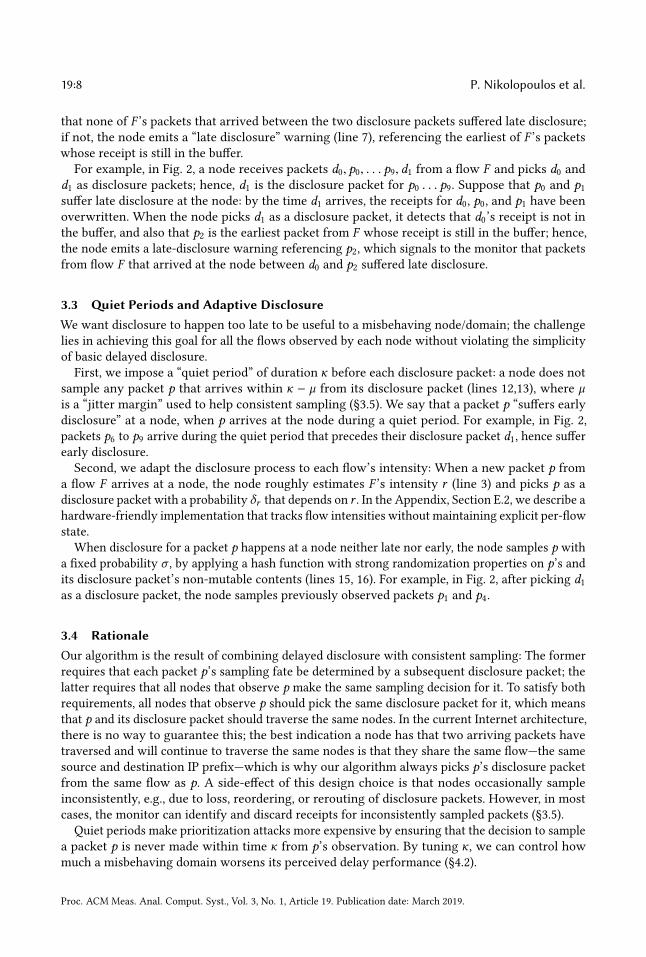
3.2 Late DisclosureWe say that a packet p “suffers late disclosure” at a node, when p’s disclosure packet arrives at thenode after p’s receipt in the node’s circular receipt buffer has been overwritten (in which case, lines
9 to 18 are never executed for p).When a node picks a new disclosure packet, it checks for late disclosure and warns the monitor.
More specifically, when a node picks a packet from a flow F as a disclosure packet, it checks whether
the receipt for the previous disclosure packet from F is still in the buffer (line 6); if yes, it is certain
Proc. ACM Meas. Anal. Comput. Syst., Vol. 3, No. 1, Article 19. Publication date: March 2019.
19:8 P. Nikolopoulos et al.
that none of F ’s packets that arrived between the two disclosure packets suffered late disclosure;
if not, the node emits a “late disclosure” warning (line 7), referencing the earliest of F ’s packetswhose receipt is still in the buffer.
For example, in Fig. 2, a node receives packets d0, p0, . . . p9, d1 from a flow F and picks d0 andd1 as disclosure packets; hence, d1 is the disclosure packet for p0 . . . p9. Suppose that p0 and p1suffer late disclosure at the node: by the time d1 arrives, the receipts for d0, p0, and p1 have beenoverwritten. When the node picks d1 as a disclosure packet, it detects that d0’s receipt is not inthe buffer, and also that p2 is the earliest packet from F whose receipt is still in the buffer; hence,
the node emits a late-disclosure warning referencing p2, which signals to the monitor that packets
from flow F that arrived at the node between d0 and p2 suffered late disclosure.
3.3 Quiet Periods and Adaptive DisclosureWe want disclosure to happen too late to be useful to a misbehaving node/domain; the challenge
lies in achieving this goal for all the flows observed by each node without violating the simplicity
of basic delayed disclosure.
First, we impose a “quiet period” of duration κ before each disclosure packet: a node does not
sample any packet p that arrives within κ − µ from its disclosure packet (lines 12,13), where µis a “jitter margin” used to help consistent sampling (§3.5). We say that a packet p “suffers early
disclosure” at a node, when p arrives at the node during a quiet period. For example, in Fig. 2,
packets p6 to p9 arrive during the quiet period that precedes their disclosure packet d1, hence sufferearly disclosure.
Second, we adapt the disclosure process to each flow’s intensity: When a new packet p from
a flow F arrives at a node, the node roughly estimates F ’s intensity r (line 3) and picks p as a
disclosure packet with a probability δr that depends on r . In the Appendix, Section E.2, we describe ahardware-friendly implementation that tracks flow intensities without maintaining explicit per-flow
state.
When disclosure for a packet p happens at a node neither late nor early, the node samples p with
a fixed probability σ , by applying a hash function with strong randomization properties on p’s andits disclosure packet’s non-mutable contents (lines 15, 16). For example, in Fig. 2, after picking d1as a disclosure packet, the node samples previously observed packets p1 and p4.
3.4 RationaleOur algorithm is the result of combining delayed disclosure with consistent sampling: The former
requires that each packet p’s sampling fate be determined by a subsequent disclosure packet; the
latter requires that all nodes that observe p make the same sampling decision for it. To satisfy both
requirements, all nodes that observe p should pick the same disclosure packet for it, which means
that p and its disclosure packet should traverse the same nodes. In the current Internet architecture,
there is no way to guarantee this; the best indication a node has that two arriving packets have
traversed and will continue to traverse the same nodes is that they share the same flow—the same
source and destination IP prefix—which is why our algorithm always picks p’s disclosure packetfrom the same flow as p. A side-effect of this design choice is that nodes occasionally sample
inconsistently, e.g., due to loss, reordering, or rerouting of disclosure packets. However, in most
cases, the monitor can identify and discard receipts for inconsistently sampled packets (§3.5).
Quiet periods make prioritization attacks more expensive by ensuring that the decision to sample
a packet p is never made within time κ from p’s observation. By tuning κ, we can control how
much a misbehaving domain worsens its perceived delay performance (§4.2).
Proc. ACM Meas. Anal. Comput. Syst., Vol. 3, No. 1, Article 19. Publication date: March 2019.
Retroactive Packet Sampling for Traffic Receipts 19:9
The adaptation of the disclosure process to each flow’s intensity regulates early and late disclosure
and ensures that each node produces enough receipts from each flow to enable accurate statistics.
Both early and late disclosure exclude packets from sampling; hence, if we want a node to sample
packets from a flow F at some minimum rate, we have to ensure that enough packets from F escape
early and late disclosure. The probability of early disclosure depends on the interplay between
F ’s intensity r , the disclosure rate δ , and the quiet-period duration κ; this interplay determines
how many of F ’s packets fall into a quiet period. The probability of late disclosure depends on the
interplay between r , δ , the rest of the traffic arriving at the node, and the size of the receipt buffer
β ; this interplay determines how quickly the receipt buffer fills up and how many of F ’s receiptsare overwritten prematurely. So, to keep the probabilities of early and late disclosure at a desired
value, we have to quantify the above interactions and continuously adapt the disclosure process to
F ’s intensity—this is why nodes track flow intensities and why δ is a function of r .
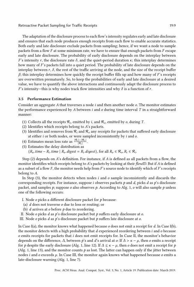
3.5 Performance EstimationConsider an aggregate A that traverses a node i and then another node o. The monitor estimates
the performance experienced by A between i and o during time interval T in a straightforward
manner:
(1) Collects all the receipts Ri, emitted by i , and Ro, emitted by o, during T .(2) Identifies which receipts belong to A’s packets.(3) Identifies and removes from Ri and Ro any receipts for packets that suffered early disclosure
at either i or both nodes, or were sampled inconsistently by i and o.
(4) Estimates mean loss rate as|Ri |− |Ro |
|Ri |.
(5) Estimates the delay distribution as
{Ro .time − Ri .time | Ro .digest = Ri .diдest}, for all Ro ∈ Ro, Ri ∈ Ri.
Step (2) depends on A’s definition. For instance, if A is defined as all packets from a flow, the
monitor identifies which receipts belong toA’s packets by looking at their flowID. But ifA is defined
as a subset of a flow F , the monitor needs help from F ’s source node to identify which of F ’s receiptsbelong to A.In Step (3), the monitor detects when nodes i and o sample inconsistently and discards the
corresponding receipts. For instance, suppose i observes packets p and d, picks d as p’s disclosurepacket, and samples p; suppose o also observes p. According to Alg. 1, o will also sample p unless
one of the following occurs:
I. Node o picks a different disclosure packet for p because:
(a) d does not traverse o due to loss or routing; or
(b) d arrives at o before p due to reordering.
II. Node o picks d as p’s disclosure packet but p suffers early disclosure at o.III. Node o picks d as p’s disclosure packet but p suffers late disclosure at o.
In Case I(a), the monitor knows what happened because o does not emit a receipt for d. In Case I(b),
the monitor detects with a high probability that d experienced reordering between i and o becauseo emits receipts for packets that i does not emit receipts for. In Case II, the monitor’s behavior
depends on the difference, ∆, between p’s and d’s arrival at o: If ∆ > κ − µ, then o emits a receipt
for p despite the early disclosure (Alg. 1, line 12). If ∆ ≤ κ − µ, then o does not emit a receipt for p(Alg. 1, line 13), and the monitor counts p as lost. The latter can happen only if the jitter between
nodes i and o exceeds µ. In Case III, the monitor again knows what happened because o emits a
late-disclosure warning (Alg. 1, line 7).
Proc. ACM Meas. Anal. Comput. Syst., Vol. 3, No. 1, Article 19. Publication date: March 2019.

19:10 P. Nikolopoulos et al.
The accuracy of the monitor’s estimates depends on the number of samples on which they are
based. Hence, the monitor picks a target (γ , ϵ)-accuracy and computes the minimum number of
samples Nγ ,ϵ needed to achieve this accuracy. For this computation, the monitor relies on standard
statistical models (Appendix, §D.1), parametrized with the minimum loss rate lossmin that the
monitor should be able to measure accurately and potentially the maximum loss burst size burstmax .
The parameter values depend on the scenario: When estimating the loss of a domain that promises
maximum loss ℓ, lossmin should be set to ≤ ℓ; the typical loss rate mentioned in today’s SLAs is
0.1% [8, 9, 23], so this is the default value we use in our examples. When assuming Gilbert loss, we
use burstmax = 2, because we experimentally found that this value is conservative even for highly
congested environments.
4 MISBEHAVIOR ANALYSISIn this section, we study prioritization attacks: we present an attack model that captures all such
attacks (§4.1) and sufficient conditions under which any prioritization attack is ineffective given
the assumptions in §2.5 (§4.2). We discuss other misbehavior in the Appendix, §B.
Attack parameters (unknown to us){lg , dg} Loss/delay of good route
{lb, db} Loss/delay of bad route
g Fraction of traffic sent over good route
t Buffering period
Symbols used in analysis{ˆlhon, ˆdhon} Loss/delay estimates if node i is honest
{ˆlmis, ˆdmis} Loss/delay estimates if node i misbehaves
ˆlhon − ˆlmis Loss benefit
ˆdhon − ˆdmis Delay benefit
F Denotes both a flow and the stationary and ergodic process of its packet arrivals at a node
P The stationary and ergodic process of all packet arrivals at a node
nF [0,κ) The number of F -points that occur within time κ after a packet p’s arrivalnF [P0 , Pβ ) The number of F -points that occur within β P-points after a packet p’s arrival
Table 2. Attack parameters and symbols.
4.1 Prioritization Attack ModelConsider a domain x with an entry node i and an exit node o, and two routes between i ando: a “good” route with mean loss and delay {lg, dg} and a “bad” route with mean loss and delay
{lb ≥ lg, db ≥ dg}. Consider a flow F that traverses node i and then node o. F ’s packet arrivals (resp.all packet arrivals) at i form a stationary, ergodic process that has intensity r (resp. R).
In a prioritization attack, node i delays forwarding F ’s packets for a maximum “buffering period”
t; if it learns a packet p’s sampling fate while p is still buffered, it forwards p over the good or bad
route accordingly. The attack is successful when the benefit from forwarding packets based on
their sampling fate outweighs the cost of buffering—hence delaying—packets.
More specifically: Node i forwards a fraction g ∈ [0, 1) of F ’s packets over the good route and
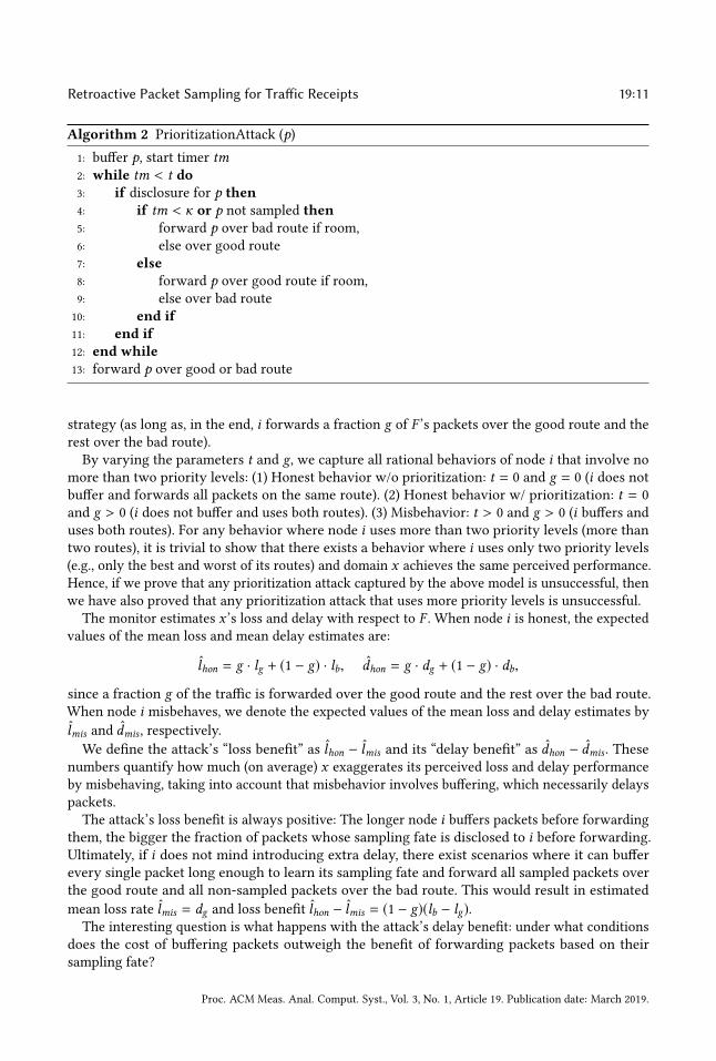
the rest over the bad route. Upon receiving a packet p, node i runs Alg. 1, then Alg. 2: It buffers pfor a maximum period t ≥ 0 (line 1). If i learns that p will not be sampled (lines 2–4), it forwards
p over the bad route if possible (lines 5,6). If i learns that p will be sampled (line 7), it forwards pover the good route if possible (lines 8,9). Finally, if the buffering period runs out before disclosure
occurs, then i forwards p over the good or the bad route (line 13) based on an arbitrary forwarding
Proc. ACM Meas. Anal. Comput. Syst., Vol. 3, No. 1, Article 19. Publication date: March 2019.
Retroactive Packet Sampling for Traffic Receipts 19:11
Algorithm 2 PrioritizationAttack (p)
1: buffer p, start timer tm2: while tm < t do3: if disclosure for p then4: if tm < κ or p not sampled then5: forward p over bad route if room,
6: else over good route
7: else8: forward p over good route if room,
9: else over bad route
10: end if11: end if12: end while13: forward p over good or bad route
strategy (as long as, in the end, i forwards a fraction g of F ’s packets over the good route and the
rest over the bad route).
By varying the parameters t and g, we capture all rational behaviors of node i that involve nomore than two priority levels: (1) Honest behavior w/o prioritization: t = 0 and g = 0 (i does notbuffer and forwards all packets on the same route). (2) Honest behavior w/ prioritization: t = 0
and g > 0 (i does not buffer and uses both routes). (3) Misbehavior: t > 0 and g > 0 (i buffers anduses both routes). For any behavior where node i uses more than two priority levels (more than
two routes), it is trivial to show that there exists a behavior where i uses only two priority levels
(e.g., only the best and worst of its routes) and domain x achieves the same perceived performance.
Hence, if we prove that any prioritization attack captured by the above model is unsuccessful, then
we have also proved that any prioritization attack that uses more priority levels is unsuccessful.
The monitor estimates x ’s loss and delay with respect to F . When node i is honest, the expectedvalues of the mean loss and mean delay estimates are:
ˆlhon = g · lg + (1 − g) · lb, ˆdhon = g · dg + (1 − g) · db,
since a fraction g of the traffic is forwarded over the good route and the rest over the bad route.
When node i misbehaves, we denote the expected values of the mean loss and delay estimates by
ˆlmis and ˆdmis , respectively.
We define the attack’s “loss benefit” asˆlhon − ˆlmis and its “delay benefit” as
ˆdhon − ˆdmis . These
numbers quantify how much (on average) x exaggerates its perceived loss and delay performance
by misbehaving, taking into account that misbehavior involves buffering, which necessarily delays
packets.
The attack’s loss benefit is always positive: The longer node i buffers packets before forwardingthem, the bigger the fraction of packets whose sampling fate is disclosed to i before forwarding.Ultimately, if i does not mind introducing extra delay, there exist scenarios where it can buffer
every single packet long enough to learn its sampling fate and forward all sampled packets over
the good route and all non-sampled packets over the bad route. This would result in estimated
mean loss rateˆlmis = dg and loss benefit
ˆlhon − ˆlmis = (1 − g)(lb − lg).The interesting question is what happens with the attack’s delay benefit: under what conditions
does the cost of buffering packets outweigh the benefit of forwarding packets based on their
sampling fate?
Proc. ACM Meas. Anal. Comput. Syst., Vol. 3, No. 1, Article 19. Publication date: March 2019.
19:12 P. Nikolopoulos et al.
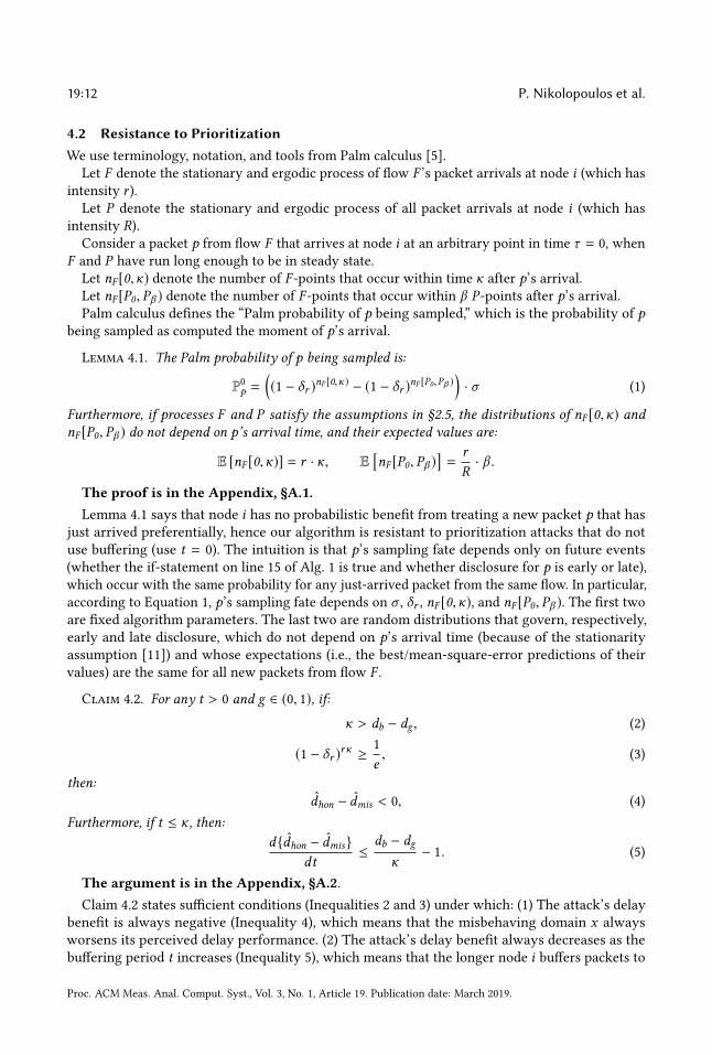
4.2 Resistance to PrioritizationWe use terminology, notation, and tools from Palm calculus [5].
Let F denote the stationary and ergodic process of flow F ’s packet arrivals at node i (which has
intensity r ).Let P denote the stationary and ergodic process of all packet arrivals at node i (which has
intensity R).Consider a packet p from flow F that arrives at node i at an arbitrary point in time τ = 0, when
F and P have run long enough to be in steady state.
Let nF [0,κ) denote the number of F -points that occur within time κ after p’s arrival.Let nF [P0, Pβ ) denote the number of F -points that occur within β P-points after p’s arrival.Palm calculus defines the “Palm probability of p being sampled,” which is the probability of p
being sampled as computed the moment of p’s arrival.
Lemma 4.1. The Palm probability of p being sampled is:
P0p =((1 − δr )
nF [0,κ) − (1 − δr )nF [P0,Pβ )
)· σ (1)
Furthermore, if processes F and P satisfy the assumptions in §2.5, the distributions of nF [0,κ) andnF [P0, Pβ ) do not depend on p’s arrival time, and their expected values are:
E [nF [0,κ)] = r · κ, E[nF [P0, Pβ )
]=
r
R· β .
The proof is in the Appendix, §A.1.Lemma 4.1 says that node i has no probabilistic benefit from treating a new packet p that has
just arrived preferentially, hence our algorithm is resistant to prioritization attacks that do not
use buffering (use t = 0). The intuition is that p’s sampling fate depends only on future events
(whether the if-statement on line 15 of Alg. 1 is true and whether disclosure for p is early or late),
which occur with the same probability for any just-arrived packet from the same flow. In particular,
according to Equation 1, p’s sampling fate depends on σ , δr , nF [0,κ), and nF [P0, Pβ ). The first twoare fixed algorithm parameters. The last two are random distributions that govern, respectively,
early and late disclosure, which do not depend on p’s arrival time (because of the stationarity
assumption [11]) and whose expectations (i.e., the best/mean-square-error predictions of their
values) are the same for all new packets from flow F .
Claim 4.2. For any t > 0 and g ∈ (0, 1), if:
κ > db − dg, (2)
(1 − δr )rκ ≥
1
e, (3)
then:ˆdhon − ˆdmis < 0, (4)
Furthermore, if t ≤ κ, then:d{ ˆdhon − ˆdmis}
dt≤
db − dg
κ− 1. (5)
The argument is in the Appendix, §A.2.Claim 4.2 states sufficient conditions (Inequalities 2 and 3) under which: (1) The attack’s delay
benefit is always negative (Inequality 4), which means that the misbehaving domain x always
worsens its perceived delay performance. (2) The attack’s delay benefit always decreases as the
buffering period t increases (Inequality 5), which means that the longer node i buffers packets to
Proc. ACM Meas. Anal. Comput. Syst., Vol. 3, No. 1, Article 19. Publication date: March 2019.
Retroactive Packet Sampling for Traffic Receipts 19:13
gain information about their sampling fate, the worse x ’s perceived delay performance becomes. In
particular, if κ ≫ db − dg , thend { ˆdhon− ˆdmis }
d t → −1, which means that: for every msec that node ibuffers packets, it worsens x ’s perceived delay performance by almost one msec. In our opinion,
given the importance of delay for modern applications, no domain would choose to penalize its
perceived delay performance this way in order to exaggerate its loss performance.
Inequality 2 is straightforward: the quiet period should be longer than the delay difference
between the bad and good route within the misbehaving domain. The longer the quiet period,
the longer node i needs to buffer p before learning that p will be sampled. By making the quiet
period longer than the good-bad route delay difference, we ensure that i cannot compensate for
the buffering delay by sending p over the good route.
Inequality 3 is more subtle and something we did not expect—it emerged from the math: the
average fraction of packets that suffer early disclosure does not exceed 1 − 1/e. If disclosure for
p happens early (i.e., during a quiet period), node i learns that p will not be sampled and cheats
by forwarding p over the bad route. Increasing the quiet-period duration does not help control
this event—quite the contrary: longer quiet periods lead to more early-disclosure events and more
opportunities for this kind of cheating. Ultimately, the amount of packets that suffer early disclosure
could become large enough to saturate the bad route; in this case, by forwarding all packets that
suffer early disclosure over the bad route, node i ends up forwarding all packets that do not sufferearly disclosure—which include all the sampled packets—over the good route. Inequality 3 prevents
this scenario, because it regulates/upper bounds (up to 1 − 1/e) the average fraction of packets that
suffer early disclosure and could therefore be mistreated. This being a sufficient (not necessary)
condition, we do not have an intuitive explanation for why the1/e bound in particular works; it is
the tightest bound we could find that—together with Inequality 2—enabled us to prove that the
delay benefit is always negative, but a tighter bound may exist.
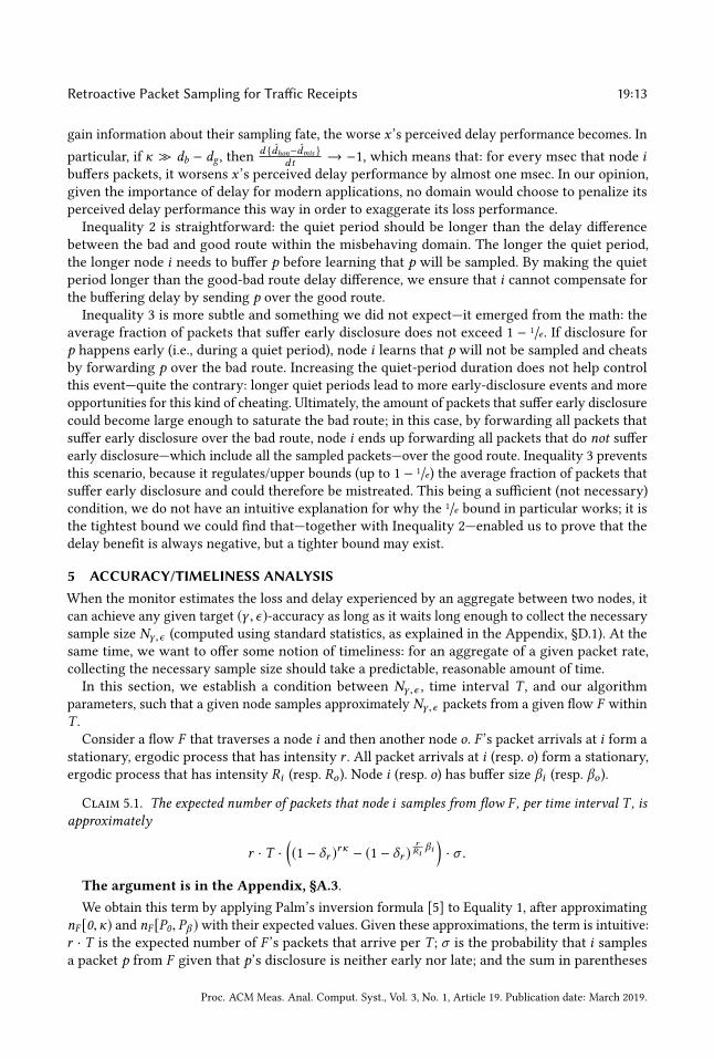
5 ACCURACY/TIMELINESS ANALYSISWhen the monitor estimates the loss and delay experienced by an aggregate between two nodes, it
can achieve any given target (γ , ϵ)-accuracy as long as it waits long enough to collect the necessary
sample size Nγ ,ϵ (computed using standard statistics, as explained in the Appendix, §D.1). At the
same time, we want to offer some notion of timeliness: for an aggregate of a given packet rate,
collecting the necessary sample size should take a predictable, reasonable amount of time.
In this section, we establish a condition between Nγ ,ϵ , time interval T , and our algorithm
parameters, such that a given node samples approximately Nγ ,ϵ packets from a given flow F within
T .Consider a flow F that traverses a node i and then another node o. F ’s packet arrivals at i form a
stationary, ergodic process that has intensity r . All packet arrivals at i (resp. o) form a stationary,
ergodic process that has intensity Ri (resp. Ro ). Node i (resp. o) has buffer size βi (resp. βo ).
Claim 5.1. The expected number of packets that node i samples from flow F , per time interval T , isapproximately
r · T ·((1 − δr )
rκ − (1 − δr )rRi
βi)· σ .
The argument is in the Appendix, §A.3.We obtain this term by applying Palm’s inversion formula [5] to Equality 1, after approximating
nF [0,κ) and nF [P0, Pβ )with their expected values. Given these approximations, the term is intuitive:
r · T is the expected number of F ’s packets that arrive per T ; σ is the probability that i samples
a packet p from F given that p’s disclosure is neither early nor late; and the sum in parentheses
Proc. ACM Meas. Anal. Comput. Syst., Vol. 3, No. 1, Article 19. Publication date: March 2019.
19:14 P. Nikolopoulos et al.
approximates the probability that p’s disclosure is neither early nor late. Approximating nF [0,κ)and nF [P0, Pβ ) with their expected values is justified by our “fast ergodic convergence” assumption
(§2.5). In the appendix, §A.3, we experimentally validate these approximations using real traffic
traces.
Hence, if we want node i to sample approximately Nγ ,ϵ packets from flow F within time interval
T , it should be the case that
Nγ ,ϵ ≤ r · T ·((1 − δr )
rκ − (1 − δr )rRi
βi)· σ . (6)
Claim 5.2. If the following conditions hold:
I. nodes i and o observe the same disclosure packets from flow F ,and disclosure packets are not reordered with any other packets between i and o;
II. the jitter between i and o is below µ;III. βi
Ri=
βoRo=
βR ;
then i and o sample F ’s packets consistently.
The argument is in the Appendix, §A.4.To be precise, the three conditions of Claim 5.2 ensure that the conditional probability that
o samples a packet p given that o observes p and i samples p is approximately (not always) 1.
Condition I ensures that i and o pick the same disclosure packet for p. Condition II ensures that,
if p does not suffer early disclosure at i and i samples p, then o will also sample p. Condition III
ensures that, if p does not suffer late disclosure at i , it will not suffer late disclosure at o either.If Conditions I and/or II do not hold
1, the monitor can still achieve its target accuracy, but it
needs to wait longer, because nodes produce consistent samples more slowly than indicated in
Claim 5.2. We discuss this in the Appendix, §C.
6 PARAMETRIZATION AND RESOURCESIn this section, we describe how to parametrize our algorithm based on our misbehavior and
accuracy/timeliness analyses (§6.1) and state the resulting resource requirements (§6.2).
6.1 Algorithm ParametrizationWe parametrize our algorithm such that each node uses the minimum buffer size necessary and
Inequalities 2, 3, and 6 are satisfied.
Selection rate σ .Recall that σ is the conditional probability with which a node samples a packet given that the
packet does not suffer early or late disclosure at the node. Hence, σ is the maximum sampling rate
that our algorithm may apply to a flow. We set σ according to the sampling capabilities of network
devices. In the current Internet, we would set σ to 1% or so, which is typically supported by modern
network devices [6].
Quiet period duration κ.We set κ according to Inequality 2 (κ ≫ db − dg), such that the delay benefit of any prioritization
attack is negative and drops quickly as the buffering period increases. Given that we cannot know
the value of db − dg for all prioritization attacks, we need to set κ conservatively, such that it is
significantly larger than any realistic intra-domain route difference. In the current Internet, we
would set κ to 100msec or so.
1Condition III is under our control, and we can make it hold.
Proc. ACM Meas. Anal. Comput. Syst., Vol. 3, No. 1, Article 19. Publication date: March 2019.
Retroactive Packet Sampling for Traffic Receipts 19:15
0 1 2 3 4 5Disclosure rate
r 10-5
106
107
Pa
cke
t ra
te r
(p
ps) lower bound from Ineq. 6
upper bound from Ineq. 6upper bound from Ineq. 3
Fig. 3. Example operational regime.
2 4 6 8 10 12 14Minimum supported rate r
min (pkts/sec) 10
5
101
102
Me
mo
ry (
MB
)
basic DDretro
Fig. 4. Receipt-buffer size as a function of rmin.
Buffer size β .(1) We pick the loss model (lossmin and—if we assume Gilbert loss—burstmax ) and the target
(γ , ϵ)-accuracy that the monitor should achieve given this model. From these, we compute the
minimum number of receipts Nγ ,ϵ that the monitor needs to collect per flow in order to compute
an estimate. The computation is in the Appendix, §D.1.
(2) We pick the time interval T , and the minimum and maximum flow intensity, rmin and rmax ,
for which the monitor should achieve the target accuracy.
Given (1) and (2), we compute the minimum value ofβR for which both Inequalities 3 and 6 are
satisfied and set each node’s buffer size accordingly. The computation is in the Appendix, §D.2.
There are two important things to note: First, for each node, we set the buffer size such that it
is sufficient for all flow intensities in [rmin, rmax]. Second, across nodes, the buffer size can differ
significantly, because it depends on the intensity R of all packet arrivals at the node.
Disclosure function r → δr .Recall that δr is the probability with which a node picks a packet from a flow of intensity r as a
disclosure packet.
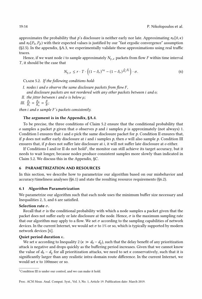
For given values of σ , κ, andβR , Inequalities 3 and 6 define the “operational regime” of our
disclosure process: the set of all possible tuples {δr , r } that make prioritization attacks ineffective
and make each node emit enough receipts in a timely manner. Fig. 3 shows an example operational
regime: it is the surface enclosed between a lower bound obtained from Inequality 6 (blue curve)
and the smallest of two upper bounds obtained, respectively, from Inequality 3 (yellow curve) and
Inequality 6 (red curve); in this particular example, the smallest upper bound is the former (the
yellow curve). The particular scenario for which we computed this operational regime does not
matter for this discussion, but we provide it for completeness: target accuracy (γ = 95%, ϵ = 10%),
target time interval T = 10min, minimum flow intensity rmin = 155Kpps (saturated OC-12 interface,
assuming average packet size 500B), maximum flow intensity rmax = 2.5Mpps (saturated OC-192
interface, assuming average packet size 500B), and algorithm parameters σ = 1%, κ = 100msec, and
β = 10.5MB.
We set our disclosure function such that any tuple {δr , r } falls in the operational regime; we
describe how in the Appendix, §D.3. Fig. 3 shows an example disclosure function (black curve) that
consists of two vertical lines: all flow intensities below 437Kpps map to disclosure rate 2.18 · 10−5,while all flow intensities above 437Kpps map to disclosure rate 0.137 · 10−5.
6.2 Resource RequirementsHaving established how to parametrize our algorithm, we considered the values we would use in
various realistic scenarios and computed the resulting resource requirements.
Proc. ACM Meas. Anal. Comput. Syst., Vol. 3, No. 1, Article 19. Publication date: March 2019.
19:16 P. Nikolopoulos et al.
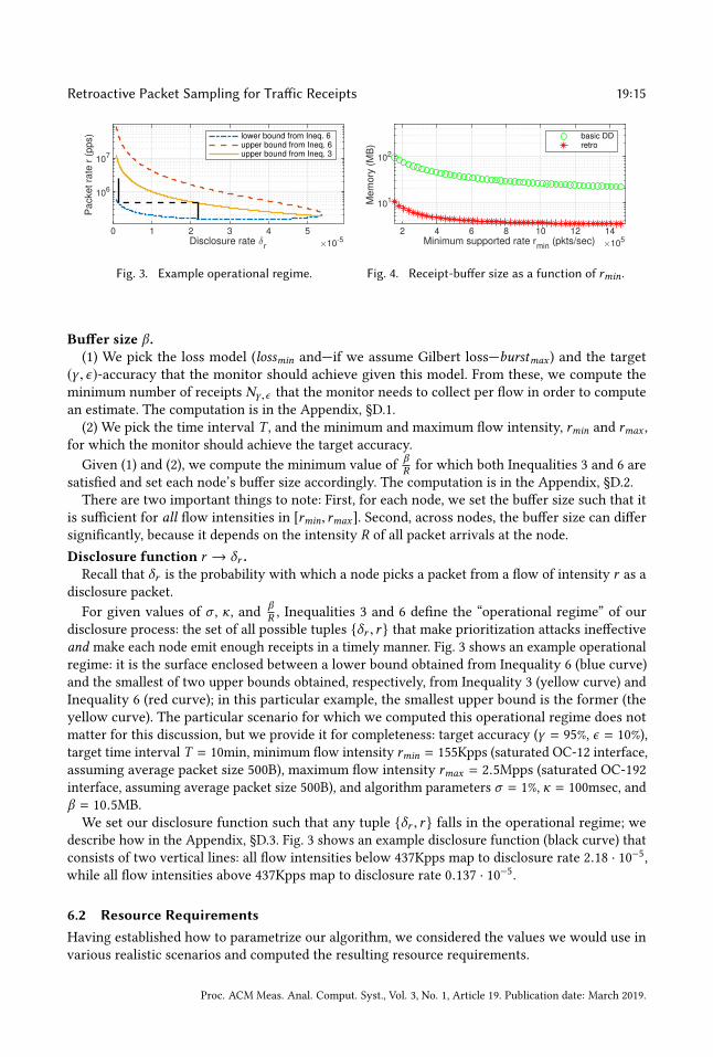
Memory overhead.We found that our algorithm requires a buffer size that increases data-path memory only by a
few percentage points, which is, in most cases, about an order of magnitude less than basic delayed
disclosure (DD).
We present a concrete example: Consider a node collocated with a 10GigE interface, observing
traffic of intensity R = 2.5Mpps with an average packet size 500B. Assume 12B per receipt (§E.1).
We set σ = 1%, κ = 100msec, lossmin = 0.1%, γ = 95%, ϵ = 10%, and T = 10min.
Fig. 4 shows the buffer size required by our algorithm versus basic DD as a function of rmin (the
minimum supported flow intensity). Our algorithm (red stars, abbrv. “retro”) requires a few MB of
data-path memory, whereas basic DD (green circles) requires about an order of magnitude more.
To put this in perspective, a 10GigE interface needs about 125MB of packet buffers (using the “one
round-trip worth of traffic” rule and assuming a typical Internet round-trip of 100msec), i.e., our
algorithm increases data-path memory by only a few percentage points.
There are three reasons why our algorithm requires less data-path memory than basic DD: (1)
Basic DD was designed to collect a target fraction of packets from each flow, not a target sample
size in a target time interval; as a result, it samples more packets than necessary. (2) Basic DD uses
a fixed disclosure rate δ , yet no single δ works well for all flows: faster flows need a lower δ to
prevent early disclosure from happening too often, while slower flows need a higher δ to prevent
late disclosure from happening too often. Basic DD picks a δ that is low enough to accommodate
the fastest flows (those with intensity close to rmax ) and, as a result, requires too much memory
to protect the slowest flows (those with intensity close to rmin) from late disclosure. (3) Basic DD
avoids late disclosure with a fixed, high probability; as a result, it avoids late disclosure more than
necessary to achieve the target accuracy in the target time interval.
Processing overhead.Our algorithm requires a small number of hash computations, timestamp comparisons, and
accesses to data-path memory per packet, which is similar to basic DD (we claim no improvement
on processing overhead). The exact numbers depend on the implementation. The hardware design
sketched in the Appendix, §E.2, requires per packet: two hash computations, a couple of timestamp
comparisons, one read and one write access to data-path SRAM, and a parallel lookup and update
to data-path CAM.
7 EXPERIMENTAL EVALUATIONAfter describing our methodology (§7.1), we demonstrate that our algorithm is useful (§7.2) and
confirm that it works as expected (§7.3) and is resistant to prioritization attacks (§7.4).
7.1 MethodologyIn each experiment, we emulate some number of target flows, crossing one or more domains. Each
target flow enters each domain at one node and exits the domain at another node; there is no packet
reordering between the nodes.
We use 1-hour backbone traces made available by CAIDA in 2016 (chicago-equinix, direction A).
Each flow observed at an entry node consists of one entire trace, while the total traffic observed at an
entry node consists of multiple traces merged into one. Why this particular emulation: The question
we are most frequently asked is how well our system would work for busy backbone routers located
at the Internet core. The traffic rate of a single CAIDA trace ranges from a few hundred Mbps
to a few Gbps; this is too low to represent the total traffic arriving at a busy backbone-router
interface, but could represent, e.g., the traffic between a source and destination prefix connected
Proc. ACM Meas. Anal. Comput. Syst., Vol. 3, No. 1, Article 19. Publication date: March 2019.
Retroactive Packet Sampling for Traffic Receipts 19:17
to the Internet through OC-48 or lightly loaded 10GigE links. By merging multiple traces—and
shifting packet timestamps such that all traces start at the same time—we created higher-rate
ingress streams.
In each experiment, we emulate either i.i.d. or bursty loss (of various rates). For the latter, we
obtained the loss pattern from an actual congested link: we created in our lab a simple topology
where 16 pairs of end-points communicated over a bottleneck GigE link, and we had each pair
exchange back-to-back TCP flows; this resulted in the bottleneck link experiencing packet loss of
average rate 4.8% and burstiness 1.52 packets.Our configuration is purposefully not realistic in all scenarios, because we want our algorithm to
operate at its limits. For instance, in a real deployment, we would set lossmin = 0.1% or so. However,
if the actual loss rate is≫ lossmin, our algorithm will use significantly more memory than necessary
to estimate this loss rate, and our results will be obviously good. Hence, in each experiment, we set
lossmin to the actual loss rate introduced in the experiment, which results in our algorithm using
the minimum memory needed to estimate this loss rate. So:
(1) In all experiments, we set the selection rate to σ = 1%, the quiet-period duration to κ =100msec, the target accuracy to (γ = 95%, ϵ = 10%), and the target time interval to T = 5min.
(2) In all experiments, we set lossmin to the actual loss rate and—when the actual loss is bursty—
burstmax to the actual loss burstiness. This way, we test how accurately the monitor estimates loss
that is at the limit of what the nodes were configured to handle.
(3) In §7.2 and §7.3, we set the minimum supported flow intensity rmin to the average packet
rate of the slowest flow involved in the experiment. This way, we test how accurately the monitor
estimates loss experienced by a flow whose packet rate is at the limit of what the nodes were
configured to handle.
(4) In §7.4, where node i launches prioritization attacks, we configure the nodes such that the
average packet rate of the target flow F falls on the upper bound of the operational regime (the
middle, yellow curve in Fig 3). This is the most challenging setting we could think of: if node ioperates close to the upper bound of the operational regime, it is possible that F ’s instant packetrate fluctuates so fast that it temporarily pushes node i out of the operational regime, where it
could potentially cheat.
7.2 Use CasesFirst, we demonstrate that our algorithm enables the monitor to draw useful conclusions about
network behavior.
In each experiment, we emulate two to four flows that enter an ISP x at node i and exit at node o.Both nodes are collocated with highly loaded 10GigE interfaces. We use four CAIDA traces. The
total traffic observed at node i consists of the four traces merged together and has a rate of 8Gbps.
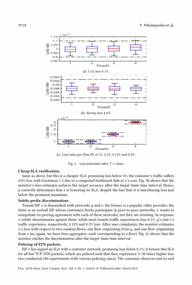
SLA verification.ISP x has signed an SLA with a customer network, promising loss below 0.1%; the customer’s
traffic suffers exactly 0.1% loss within x . On the customer’s request, the monitor estimates x ’s losswith respect to traffic from the customer’s prefix to four popular destination prefixes (so, we have
four aggregates, each corresponding to a flow). Fig. 5a shows the monitor’s loss estimates with
respect to each aggregate/flow after the target 5min time interval; in each boxplot, the red line
shows the median, while the limits of the boxplot indicate the 95% confidence interval. We see that
all estimates achieve the target accuracy (γ = 95%, ϵ = 10%). Hence, y correctly determines that xis borderline violating its SLA.
Proc. ACM Meas. Anal. Comput. Syst., Vol. 3, No. 1, Article 19. Publication date: March 2019.
19:18 P. Nikolopoulos et al.
FlowID
1 2 3 4
Loss
rat
e
×10-3
0.85
0.9
0.95
1
1.05
1.1
1.15
(a) I.i.d. loss 0.1%.
FlowID
1 2 3 4
Loss
rate
0.042
0.044
0.046
0.048
0.05
0.052
0.054
(b) Bursty loss 4.8%.
FlowID
1 2 3 4
Loss
rat
e
×10-3
1
1.5
2
2.5
3
(c) Loss rates per flow ID: 0.1%, 0.1%, 0.15% and 0.3%.
Fig. 5. Loss estimates after T = 5min.
Cheap SLA verification.Same as above, but this is a cheaper SLA, promising loss below 5%; the customer’s traffic suffers
4.8% loss with burstiness 1.5 due to a congested bottleneck link at x ’s core. Fig. 5b shows that themonitor’s loss estimates achieve the target accuracy after the target 5min time interval. Hence,
y correctly determines that x is honoring its SLA, despite the fact that it is introducing loss just
below the promised maximum.
Subtle prefix discrimination.Transit ISP x is dissatisfied with networks y and z: the former is a popular video provider; the
latter is an eyeball ISP whose customers freely participate in peer-to-peer networks; x wants to
renegotiate its peering agreement with each of these networks, but they are resisting. In response,
x subtly discriminates against them: while most transit traffic experiences loss 0.1%, y’s and z’straffic experience, respectively, 0.15% and 0.3% loss. After user complaints, the monitor estimates
x ’s loss with respect to two random flows, one flow originating from y, and one flow originating
from z (so, again, we have four aggregates, each corresponding to a flow). Fig. 5c shows that the
monitor catches the discrimination after the target 5min time interval.
Policing of SYN packets.ISP x has signed an SLA with a customer network, promising loss below 0.1%; it honors this SLA
for all but TCP SYN packets, which are policed such that they experience 3–30 times higher loss
(we conducted 240 experiments with various policing rates). The customer observes end-to-end
Proc. ACM Meas. Anal. Comput. Syst., Vol. 3, No. 1, Article 19. Publication date: March 2019.
Retroactive Packet Sampling for Traffic Receipts 19:19
ysiys oys
ydiyd oyd
xsixs oxs
xdixs oxs
did
sos
10GigE 40GigE 100GigE 40GigE 10GigE
Fig. 6. Topology emulated in §7.3.
that something is wrong with connection setup and asks the monitor whether x is discriminating
against its SYN packets. In response, the monitor defines two aggregates: SYN packets from the
customer’s prefix to some popular destination prefix; all other packets with the same source and
destination prefix. So, in this case, we have two aggregates that are subsets of the same flow.
The challenge is that the SYN aggregate is relatively small, and the monitor would need to collect
receipts for hours in order to estimate x ’s loss with respect to the SYN aggregate with the target
accuracy of (γ = 95%, ϵ = 10%). However, the goal here is not to estimate x ’s performance, but to
determine whether it treated the two aggregates differently. This can be done much faster, with a
simple Maximum Likelihood differentiation detector: the monitor estimates x ’s loss rate for eachaggregate based on the receipts it collects within some period of time (minutes, not hours); and
computes the corresponding confidence intervals (CI); if the lower limit of the CI for the SYN
aggregate estimate is greater than the upper limit of the CI for the no-SYN aggregate, then the
monitor concludes that x discriminates against the SYN aggregate.
Our results, after the target 5min time interval: When x ’s loss with respect to SYN packets is 5 or
more times higher, the monitor detects differentiation with probability 100% (in all experiment runs);
when SYN loss is 3–5 times higher, detection rate is ≥ 94%; for subtler differentiation, detection
rate drops sharply. For completeness, we also ran 480 experiments where x does not differentiate,
and the monitor correctly detects no differentiation.
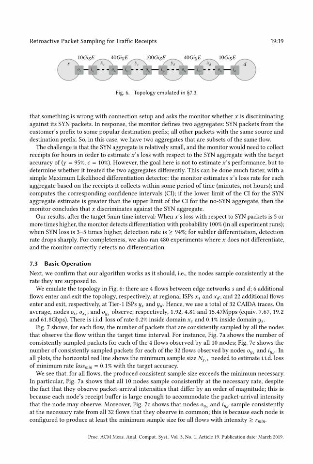
7.3 Basic OperationNext, we confirm that our algorithm works as it should, i.e., the nodes sample consistently at the
rate they are supposed to.
We emulate the topology in Fig. 6: there are 4 flows between edge networks s and d ; 6 additionalflows enter and exit the topology, respectively, at regional ISPs xs and xd ; and 22 additional flows
enter and exit, respectively, at Tier-1 ISPs ys and yd . Hence, we use a total of 32 CAIDA traces. On
average, nodes os , oxs , and oys observe, respectively, 1.92, 4.81 and 15.47Mpps (equiv. 7.67, 19.2and 61.8Gbps). There is i.i.d. loss of rate 0.2% inside domain xs and 0.1% inside domain ys .
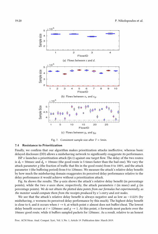
Fig. 7 shows, for each flow, the number of packets that are consistently sampled by all the nodes
that observe the flow within the target time interval. For instance, Fig. 7a shows the number of
consistently sampled packets for each of the 4 flows observed by all 10 nodes; Fig. 7c shows the
number of consistently sampled packets for each of the 32 flows observed by nodes oys and iyd . Inall plots, the horizontal red line shows the minimum sample size Nγ ,ϵ needed to estimate i.i.d. loss
of minimum rate lossmin = 0.1% with the target accuracy.
We see that, for all flows, the produced consistent sample size exceeds the minimum necessary.
In particular, Fig. 7a shows that all 10 nodes sample consistently at the necessary rate, despite
the fact that they observe packet-arrival intensities that differ by an order of magnitude; this is
because each node’s receipt buffer is large enough to accommodate the packet-arrival intensity
that the node may observe. Moreover, Fig. 7c shows that nodes oys and iyd sample consistently
at the necessary rate from all 32 flows that they observe in common; this is because each node is
configured to produce at least the minimum sample size for all flows with intensity ≥ rmin.
Proc. ACM Meas. Anal. Comput. Syst., Vol. 3, No. 1, Article 19. Publication date: March 2019.
19:20 P. Nikolopoulos et al.
1 2 3 4
FlowID
2
3
4
5
Sam
ple
size
105
(a) Flows between s and d .
1 2 3 4 5 6 7 8 9 10
FlowID
2
3
4
5
Sam
ple
size
105
(b) Flows between xs and xd .
1 5 10 15 20 25
FlowID
4
4.5
5
Sam
ple
Siz
e
105
(c) Flows between ys and yd .
Fig. 7. Consistent sample size after T = 5min.
7.4 Resistance to PrioritizationFinally, we confirm that our algorithm makes prioritization attacks ineffective, whereas basic
delayed disclosure (DD) allows a misbehaving network to significantly exaggerate its performance.
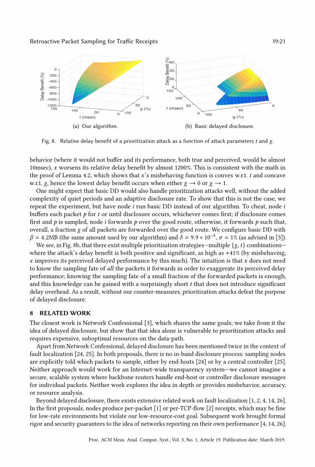
ISP x launches a prioritization attack (§4.1) against one target flow. The delay of the two routes
is db = 50msec and dg = 10msec (the good route is 5 times faster than the bad one). We vary the
attack parameter g (the fraction of traffic that fits in the good route) from 0 to 100%, and the attack
parameter t (the buffering period) from 0 to 120msec. We measure the attack’s relative delay benefit:
by how much the misbehaving domain exaggerates its perceived delay performance relative to the
delay performance it would achieve without a prioritization attack.
Fig. 8a shows the results. The y-axis shows the attack’s relative delay benefit (in percentage
points), while the two x-axes show, respectively, the attack parameters t (in msec) and g (in
percentage points). We do not obtain the plotted data points from our formulas but experimentally, asthe monitor would compute them from the receipts produced by x ’s entry and exit nodes.We see that the attack’s relative delay benefit is always negative and as low as −1122% (by
misbehaving, x worsens its perceived delay performance by this much). The highest delay benefit
is close to 0, and it occurs when t → 0, at which point x almost does not buffer/cheat. The lowest
delay benefit occurs at t = 120msec and g → 1. At this point, x forwards most packets over the
10msec good route, while it buffers sampled packets for 120msec. As a result, relative to an honest
Proc. ACM Meas. Anal. Comput. Syst., Vol. 3, No. 1, Article 19. Publication date: March 2019.
Retroactive Packet Sampling for Traffic Receipts 19:21
g (%)
0
50
100050
t (msec)
100150
0
-200
-400
-600
-800
-1000
-1200
Del
ay B
enef
it (%
)
(a) Our algorithm.
0
g (%)
501000
50t (msec)
100
60
40
20
0150
Delay
Ben
efit (%
)
(b) Basic delayed disclosure.
Fig. 8. Relative delay benefit of a prioritization attack as a function of attack parameters t and g.
behavior (where it would not buffer and its performance, both true and perceived, would be almost
10msec), x worsens its relative delay benefit by almost 1200%. This is consistent with the math in
the proof of Lemma 4.2, which shows that x ’s misbehaving function is convex w.r.t. t and concave
w.r.t. g, hence the lowest delay benefit occurs when either g → 0 or g → 1.
One might expect that basic DD would also handle prioritization attacks well, without the added
complexity of quiet periods and an adaptive disclosure rate. To show that this is not the case, we
repeat the experiment, but have node i run basic DD instead of our algorithm. To cheat, node ibuffers each packet p for t or until disclosure occurs, whichever comes first; if disclosure comes
first and p is sampled, node i forwards p over the good route, otherwise, it forwards p such that,
overall, a fraction g of all packets are forwarded over the good route. We configure basic DD with
β = 4.2MB (the same amount used by our algorithm) and δ = 9.9 ∗ 10−5, σ = 1% (as advised in [3]).
We see, in Fig. 8b, that there exist multiple prioritization strategies—multiple {g, t} combinations—
where the attack’s delay benefit is both positive and significant, as high as +41% (by misbehaving,
x improves its perceived delayed performance by this much). The intuition is that x does not need
to know the sampling fate of all the packets it forwards in order to exaggerate its perceived delay
performance; knowing the sampling fate of a small fraction of the forwarded packets is enough,
and this knowledge can be gained with a surprisingly short t that does not introduce significantdelay overhead. As a result, without our counter-measures, prioritization attacks defeat the purpose
of delayed disclosure.
8 RELATEDWORKThe closest work is Network Confessional [3], which shares the same goals; we take from it the
idea of delayed disclosure, but show that that idea alone is vulnerable to prioritization attacks and
requires expensive, suboptimal resources on the data-path.
Apart from Network Confessional, delayed disclosure has been mentioned twice in the context of
fault localization [24, 25]. In both proposals, there is no in-band disclosure process: sampling nodes
are explicitly told which packets to sample, either by end-hosts [24] or by a central controller [25].
Neither approach would work for an Internet-wide transparency system—we cannot imagine a
secure, scalable system where backbone routers handle end-host or controller disclosure messages
for individual packets. Neither work explores the idea in depth or provides misbehavior, accuracy,
or resource analysis.
Beyond delayed disclosure, there exists extensive related work on fault localization [1, 2, 4, 14, 26].
In the first proposals, nodes produce per-packet [1] or per-TCP-flow [2] receipts, which may be fine
for low-rate environments but violate our low-resource-cost goal. Subsequent work brought formal
rigor and security guarantees to the idea of networks reporting on their own performance [4, 14, 26].
Proc. ACM Meas. Anal. Comput. Syst., Vol. 3, No. 1, Article 19. Publication date: March 2019.
19:22 P. Nikolopoulos et al.
These proposals show that any fault can be localized to a link between two subsequent reporting
nodes—even when there is no centralized monitor, and networks may tamper both with packet
contents and with the receipts produced by other networks. However, these proposals focus on
fault localization for specific “paths” (in our context, a path would correspond to a flow) and require
nodes to keep per-path state. This is something that we cannot afford given our goals (§2.2, §2.3).
9 CONCLUSIONSWe proposed a packet sampling algorithm that prevents the network node that performs the
sampling from treating the sampled packets preferentially. Our algorithm is a building block for
a network transparency system, where domains produce receipts for a small sample of observed
packets, and an independent monitor collects each domain’s receipts and uses them to estimate
the domain’s mean loss rate and delay distribution quantiles. Our algorithm builds on delayed
disclosure—where the sampling function is disclosed to the sampling node with a delay—and
enhances it with quiet periods, during which sampling is disallowed, and a disclosure process
that adapts to each flow’s packet rate. These two techniques together ensure that a misbehaving
domain that tries to bias the sample to exaggerate its perceived performance instead worsens it.
Our algorithm can be configured to emit enough receipts to achieve a target accuracy within a
target time interval, while using the minimum amount of data-path memory necessary—which
ends up being a few MB of data-path memory per 10Gbps of forwarding capacity.
Acknowledgments.We deeply thank Ovidiu Mara, who did experiments to help us calibrate
our bursty loss model, the SIGMETRICS reviewers for their feedback, and our shepherd, Daniel
Figueiredo, for his extraordinary patience and level of involvement that helped significantly improve
our paper.
Proc. ACM Meas. Anal. Comput. Syst., Vol. 3, No. 1, Article 19. Publication date: March 2019.
Retroactive Packet Sampling for Traffic Receipts 19:23
REFERENCES[1] Katerina Argyraki, Petros Maniatis, David Cheriton, and Scott Shenker. 2004. Providing Packet Obituaries. In Proc. of
the ACM Workshop on Hot Topics in Networking (HotNets).[2] Katerina Argyraki, Petros Maniatis, Olga Irzak, Subramanian Ashish, and Scott Shenker. 2007. Loss and Delay
Accountability for the Internet. In Proc. of the IEEE International Conference on Network Protocols (ICNP).[3] Katerina Argyraki, Petros Maniatis, and Ankit Singla. 2010. Verifiable Network-performance Measurements. In Proc.
of the International Conference on emerging Networking EXperiments and Technologies (CoNEXT).[4] Boaz Barak, Sharon Goldberg, and David Xiao. 2008. Protocols and Lower Bounds for Failure Localization in the Internet.
In Proc. of the International Conference on the Theory and Applications of Cryptographic Techniques (EUROCRYPT).[5] Jean-Yves Le Boudec. 2011. Performance Evaluation of Computer and Communication Systems. EFPL Press.
[6] Cisco. 2019. IOS NetFlow. (2019). Retrieved January 2019 from http://www.cisco.com/c/en/us/products/ios-nx-os-
software/ios-netflow/index.html
[7] Global Net Neutrality Coalition. 2019. Status of Net Neutrality Around the World. (2019). Retrieved January 2019 from
https://www.thisisnetneutrality.org/
[8] Cogent. 2016. Network Services SLA Global. (2016). Retrieved January 2019 from https://cogentco.com/files/docs/
network/performance/global_sla.pdf
[9] Comcast. 2009. Service Level Agreement for Wholesale Dedicated Internet. (2009). Retrieved January
2019 from https://portals.comcasttechnologysolutions.com/sites/default/files/service_level_agreement_for_wholesale_
dedicated_internet_sla07292014.pdf
[10] European Commission. 2013. On-line public consultation on “specific aspects of transparency, traffic management and
switching in an Open Internet”. (2013). Retrieved January 2019 from https://ec.europa.eu/digital-single-market/en/
news/answers-public-consultation-specific-aspects-transparency-traffic-management-and-switching-open
[11] David Cox and P A. W. Lewis. 1966. The statistical analysis of series of events. Springer. 59–60 pages.[12] DPDK. 2015. Data Plane Development Kit. (2015). Retrieved May 2015 from http://dpdk.org
[13] Nick Duffield and Matthias Grossglauser. 2001. Trajectory Sampling for Direct Traffic Observation. IEEE/ACMTransactions on Networking (June 2001).
[14] Sharon Goldberg, David Xiao, Eran Tromer, Boaz Barak, and Jennifer Rexford. 2008. Path-quality Monitoring in the
Presence of Adversaries. In Proc. of the ACM International Conference on Measurement and Modeling of ComputerSystems (SIGMETRICS).
[15] Shay Gueron. 2010. Intel Advanced Encryption Standard (AES) New Instruction Set. (2010). Retrieved January 2019
from https://software.intel.com/sites/default/files/article/165683/aes-wp-2012-09-22-v01.pdf
[16] Gerhard Hasslinger and Oliver Hohlfeld. 2008. The Gilbert-Elliott Model for Packet Loss in Real Time Services on the
Internet. In Proc. of the GI/ITG Conference - Measurement, Modelling and Evalutation of Computer and CommunicationSystems (MMB).
[17] Manish Joshi and Theyazn Hassn Hadi. 2015. A Review of Network Traffic Analysis and Prediction Techniques. (2015).
arXiv:arXiv:1507.05722
[18] Myungjin Lee, Nick Duffield, and Ramana Rao Kompella. 2010. Two Samples Are Enough: Opportunistic Flow-
level Latency Estimation Using Netflow. In Proc. of the IEEE International Conference on Computer Communications(INFOCOM).
[19] William Lehr, Erin Kenneally, and Steven Bauer. 2015. The Road to an Open Internet is Paved with Pragmatic Disclosure
and Transparency Policies. In Proc. of the Telecommunications Policy Research Conference (TPRC).[20] Body of European Regulators for Electronic Communications (BEREC). 2016. BoR (16) 127: Guidelines on the
Implementation by National Regulators of European Net Neutrality Rules. (2016). Retrieved January 2019
from http://berec.europa.eu/eng/document_register/subject_matter/berec/download/0/6160-berec-guidelines-on-the-
implementation-b_0.pdf
[21] Christos Pappas, Katerina Argyraki, Stefan Bechtold, and Adrian Perrig. 2015. Transparency Instead of Neutrality. In
Proc. of the ACM Workshop on Hot Topics in Networks (HotNets).[22] Joel Sommers, Paul Barford, Nick Duffield, and Amos Ron. 2007. Accurate and Efficient SLA Compliance Monitoring.
SIGCOMM Computer Communication Review (Oct 2007).
[23] Verizon. 2019. Global Latency and Packet Delivery SLA. (2019). Retrieved January 2019 from http://www.
verizonenterprise.com/terms/global_latency_sla.xml
[24] Xin Zhang, Abhishek Jain, and Adrian Perrig. 2008. Packet-dropping Adversary Identification for Data Plane Security.
In Proc. of the International Conference on emerging Networking EXperiments and Technologies (CoNEXT).[25] Xin Zhang, Chang Lan, and Adrian Perrig. 2012. Secure and Scalable Fault Localization Under Dynamic Traffic Patterns.
In Proc. of the IEEE Symposium on Security and Privacy (SP).[26] Xin Zhang, Zongwei Zhou, Hsu-Chun Hsiao, Adrian Perrig, and Patrick Tague. 2012. ShortMAC: Efficient Data Plane
Fault Localization. In Proc. of the NDSS Symposium (NDSS).
Proc. ACM Meas. Anal. Comput. Syst., Vol. 3, No. 1, Article 19. Publication date: March 2019.
19:24 P. Nikolopoulos et al.
[27] Tanja Zseby and Sebastian Zander. 2001. Evaluation of Building Blocks for Passive One-way-delay Measurements. In
Proc. of the workshop on Passive and Active Measurement (PAM).
A PROOFSA.1 Proof of Lemma 4.1Palm sampling probability. Let Xp denote the number of F -points until p’s disclosure packet
arrives (which is also an F -point occurrence). nF [0,κ) denotes the number of F -points that occurwithin a time interval κ after τ = 0; nF [P0, Pβ ) denotes the number of F -points that occur withinthe upcoming β P-points after p.Packet p is sampled when the following three events occur: (a) the disclosure of p is not early,
i.e., Xp > nF [0,κ); (b) neither is it late, i.e., Xp ≤ nF [P0, Pβ ); and (c), p is selected by line 15 of Alg. 1.
Therefore, p’s sampling probability P0(a,b, c), as computed at time τ = 0 is given by the chain rule
of probability:
P0(a,b, c) = P(a) · P(b |a) · P(c |a,b) (7)
The last part P(c |a,b) of Eq. 7 is equal to the selection rate σ . The first two parts are computed
based on the following observation: In Alg. 1, DiscHash has strong randomization properties, which
means that the arrivals of the disclosure packets occur independently over the F -arrivals and with
equal probability δr . I.e., the disclosure arrivals form a Bernoulli stochastic process on the top of
F -arrivals, which is renewed at each F -point. Therefore, for any arbitrary packet p of flow F , the“distance” until the disclosure packet Xp, counted in F -points, follows the geometric distribution:
P(a) · P(b |a) =
= P(Xp > nF [0,κ)
)· P
(Xp ≤ nF [P0, Pβ ) | Xp > nF [0,κ)
)= P
(Xp > nF [0,κ)
)·(1 − P
(Xp > nF [P0, Pβ ) | Xp > nF [0,κ)
) )= P
(Xp > nF [0,κ)
)·(1 − P
(Xp > nF [P0, Pβ ) − nF [0,κ)
) )= (1 − δr )
nF [0,κ) ·
(1 − (1 − δr )
nF [P0,Pβ )−nF [0,κ))
= (1 − δr )nF [0,κ) − (1 − δr )
nF [P0,Pβ ), (8)
where the third derivation step is because of the memoryless property of the geometric distribution.
Given Eq. 7 and 8, the sampling probability of packet p is:
P0(a,b, c) =((1 − δr )
nF [0,κ) − (1 − δr )nF [P0,Pβ )
)· σ (9)
Independence from p’s arrival time. This is an immediate consequence of the stationarity as-
sumption made in Section §2.5. Stationarity of point processes implies that: the distribution of
the number of points in a fixed interval (τ ′1,τ ′′
1] is invariant under translation, i.e., is the same for
(τ ′1+ h,τ ′′
1+ h] for all h. It depends only on the length of the interval and not its time origin [11].
Therefore, the distributions of the number of points nF [0,κ) and nF [P0, Pβ ) depend only on κ and βand not on the time that p is observed. They are the same at any arbitrary point in time τ = 0.
Expected values of nF [P0, Pβ ) and nF [0,κ). The expected values of nF [0,κ) and nF [P0, Pβ ) arecomputed using Palm Calculus [5]:
E [nF [0,κ)] = r · κ (10)
E[nF [P0, Pβ )
]=
r
R· β (11)
Proc. ACM Meas. Anal. Comput. Syst., Vol. 3, No. 1, Article 19. Publication date: March 2019.
Retroactive Packet Sampling for Traffic Receipts 19:25
Eq. 10 is an immediate consequence of the definition of the intensity of a stationary point process,
which is equal to the expected number of points per time unit. Eq. 11 requires the following auxiliary
lemma A.1, and linearity of expectation.
Lemma A.1. Given two point processes P and F of the same stationary process, which have rates Rand r , respectively, the probability of an arbitrary P-arrival to be an F -arrival (i.e the arrived packetbelongs to flow F ), is:
πF =r
R
Proof : P and F are two point processes of the same stationary continuous-time arrival process.
Their intensities (R and r ) are just two different event “clocks” of that process: P-clock ticks every
time that a packet arrives and F -clock ticks only if the arriving packet belongs to flow F . Let λF (P)denote the intensity of the P point process measured with the event clock F . Also, let nF [P0, P1]denote the number of points of process F that fall between the two random subsequent P points P0and P1.We apply Neveu’s Exchange Theorem [5] to obtain:
λF (P) =R
r(12)
E [nF [P0, P1)] =1
λF (P).
Note that nF [P0, P1) is 1, if the packet at P0 is an F packet (i.e., if the P-point at P0 is also an
F -point), and 0 otherwise. Hence, E [nF [P0, P1)] is the probability πF that an arbitrary packet is a
packet from flow F . Thus:
πF =λ(F )
λ(P)=
r
R■
Three notes are important:
Note 1: The geometric distribution requires only an integer exponent of (1 − δr ). This is becausein the PMF of a geometrically distributed random variable the exponent denotes the number of trials
until the success, which must be an integer. But, in our case, rκ andrR β are not necessarily integer
values. Another way for computing the probabilities P(a) and P(b |a) would be to regard the arrivalsof the disclosure packets as a Poisson arrival process, which is the continuous-time equivalent
of the Bernoulli. In this case, X would be exponentially distributed with rate δr . However, if theexponents of the geometric distribution are generally large and the probability δr is relatively small
(which holds in our case as shown in Fig. 3), then the probabilities obtained using the geometric
distribution approximate very well the ones obtained by the exponential distribution. In this work,
we have used the geometric distribution, because we believe it provides more intuitive results. A
similar analysis holds when considering a Poisson arrival process for the disclosure packets.
Note 2: Lemmas 4.1 and A.1 do not imply any assumption about independence of F -arrivals,nor Poisson packet arrivals. The proofs are based on Palm Calculus and linearity of expectation,
that do not require independence. The only assumptions here are stationarity and ergodicity. The
“steady-rate”or the Poisson assumption make the computation of Eq. 11 easier and provide a good
insight of the proof, but do not correspond to real traffic arrival patterns.
Note 3–clarification about the implication of Lemma 4.1: The best prediction for nF [P0, Pβ ) andnF [0,κ) is obtained from their expected values. This is because if one wants to predict any random
variable from its distribution, then the mean-square-error (MSE) predictor and the best one-number
guess is just its expected value. By applying Eqs. 10 and 11 to Eq. 9, we get the best prediction of
the sampling probability of an arbitrary packet p, as computed at the time of arrival (Palm sampling
Proc. ACM Meas. Anal. Comput. Syst., Vol. 3, No. 1, Article 19. Publication date: March 2019.

19:26 P. Nikolopoulos et al.
probability). The latter does not depend on p’s arrival time, only on the intensities R and r . Even if
node i knows perfectly R and r , when it attempts to predict the sampling probability of each new
packet p that it observes, it computes the same sampling probability for all new packets.
A.2 Argument for Claim 4.2Our argument consists of an analysis (w.r.t. t and g) of the expected delay benefit that a misbehaving
node i (or, better stated, its domain) has, when launching a prioritization attack. For the analysis,
we consider all possible cases for t > 0 and g ∈ (0, 1) and show that Ineq. 2, 3 are sufficient to make
the expected misbehavior benefit negative, i.e. they imply Ineq. 4:
MBd ≡ ˆdhon − ˆdmis < 0
Note that in our context, it is enough to provide attack-resistance guarantees based on expecta-
tions. The actual delay benefit cannot be known to any node in advance; it can be computed only
at the end of the measurement. So, we can safely assume that if a node will launch a prioritization
attack, only if its expected misbehavior benefit is non-negative.
Case a: t ≥ κ. In this misbehavior scenario, node i is able to identify all packets for whichdisclosure happens inside the quiet period (and are therefore excluded from the sampling process),
all packets for which disclosure happens outside the quiet period (out of which samples are picked),
and some of the samples.
The exact computation of the expected misbehavior benefit depends on the forwarding strategy
that node i follows, but we can commute an upper bound. Since t ≥ κ, the monitor’s delay estimate
cannot be less than sum of κ (which is the minimum buffering time period in this case), and the
delay of the good route (which is achieved when the node manages to forward all samples over the
good route), i.e.:
ˆdmis ≥ dg + κ .
Therefore,
MBd ≡ ˆdhon − ˆdmis
= g · dg + (1 − g) · db − ˆdmis
≤ (1 − g)(db − dg
)− κ
(2)< −g∆d ≤ 0,
which means that Ineq. 2 implies Ineq. 4; i.e., the condition about κ given by Ineq. 2 is sufficient to
guarantee that a prioritization attack of Case (a) is unsuccessful.
Case b: t < κ. For this part, we divide the packets forwarded by a misbehaving node i thatlaunches the prioritization attack into two categories:
• Category I: The packets for which disclosure happens within t. Node i knows that these areexcluded from the sampling process, because they fall into the quiet period κ, and it forwardsthem over the bad route.
• Category II: The packets for which disclosure does not happen within t (hence, each of them
is buffered for t before being forwarded). Node i knows that a subset of these will not beexcluded, and a subset of the non-excluded ones will be sampled, but it does not know which
subsets these are. Hence, it forwards as many as it can over the good route and the rest over
the bad route.
Proc. ACM Meas. Anal. Comput. Syst., Vol. 3, No. 1, Article 19. Publication date: March 2019.
Retroactive Packet Sampling for Traffic Receipts 19:27
Misbehavior Benefit Function. Let ∆d = db − dg be the delay difference of the two routes and m(t)denote the expected fraction of packets for which disclosure happens within t (packets of CategoryI described above). Let also t⋆, denote the buffering time at which the bad route is saturated with
packets whose disclosure happens during their buffering period and therefore their exclusion for
the sampling process is verified by the misbehaving node. I.e.:
m(t⋆) = 1 − g (13)
Given the attack model that is described in §4.1, for any g ∈ (0, 1), the expected misbehavior
benefit takes the following form w.r.t. t:
MBd =
{gm(t)1−m(t)∆d − t if 0 < t ≤ t⋆
(1 − g)∆d − t if t ≥ t⋆(14)
Computation of the upper branch of Eq. 14: Due to its definition, m(t) is an increasing function of
t. Hence:
m(t) ≤ m(t⋆)(17)⇐⇒m(t) ≤ 1 − g
⇔g
1 −m(t)≤ 1 (15)
Ineq. 15 shows that the packets of Category II exceed or exactly match the capacity of the good
route. In this case, the node forwards as many of these packets as it can (i.e.g
1−m(t) ) over the good
route and the rest (i.e. 1−g
1−m(t) ) over the bad route. It does so, because this is the only way it never
exceeds the capacities of both routes and it maximizes the number of packets of Category II (from
which the sample will be selected) that follow the good route.
Note that the exact algorithm, with which the node manages to perform the above policy at line
rates, is not required for this proof. I.e. we consider here the best possible misbehaving scenario
that is offered to the node because of the domain’s network conditions. This makes our analysis a
worst-case approach.The monitor always produces an accurate delay estimate, based on a sample of packets of
Category II. Hence, the expected2value of estimated mean delay of the domain is:
ˆdmis =g
1 −m(t)(dg + t
)+
(1 −
g1 −m(t)
)(db + t) (16)
Based on Eq. 16, we obtain the upper branch of Eq. 14:
MBd =g · dg + (1 − g) · db − ˆdmis
(16)= −
g − gm(t) − g1 −m(t)
dg − t
+1 − g −m(t) + gm(t) − 1 + g +m(t)
1 −m(t)db
=gm(t)
1 −m(t)∆d − t, ∀t ∈ [
0, t⋆].
2The exact estimate cannot be known in advance, because it is produced from the collected sample, but the estimate will be
very close to the expected value. This is because the number of packets of Category II is smaller than the total flow traffic.
This, in turn, means that the collected sample (as computed in §D.1) is larger than necessary to estimate the average delay
of those packets with adequate accuracy. By fixing γ and ϵ to reasonable values (e.g. γ = 95% and ϵ = 10%), the accuracy of
ˆdmis is, almost surely, adequately high.
Proc. ACM Meas. Anal. Comput. Syst., Vol. 3, No. 1, Article 19. Publication date: March 2019.
19:28 P. Nikolopoulos et al.
Computation of the lower branch of Eq. 14: At the buffering time t = t⋆, the capacity of the
bad route is saturated with packets of Category I, and, because of Eq. 17, the misbehavior benefit
becomes MBd (t⋆) = (1 − g)∆d − t⋆. I.e. all sampled packets follow the good route.
If the node buffers for time t > t⋆, then the packets will be delayed for more time, while
all non-excluded packets will continue to follow the good route. So,ˆdmis = dg + t and thus
MBd = (1 − g)∆d − t.
Upper bound for Eq. 14: We can compute an upper bound for the expected misbehavior benefit
by finding an upper bound for the expected fraction of packets of Category I, i.e., m(t).Given a disclosure probability δr and a buffering period t, for any packet from flow F that
arrives at time t0, the probability that its disclosure packet arrives within period t follows thegeometric distribution with parameter δr , and it is equal to: 1−(1−δr )
nF [t0,t0+t), where nF [t0, t0 + t)
is the number of packets from flow F that fall inside the time interval [t0, t0 + t). Therefore, sincenF [t0, t0 + t) is random variable, the actual fraction of packets of Category I is also a random
variable.
An upper bound for m(t) can be found using our stationarity assumption and (§2.5) Jensen’s
Inequality: Flow F ’s packet arrivals form a stationary and ergodic point process with intensity r .Therefore, nF [t0, t0 + t] is a random variable whose distribution is invariant under time shifts, i.e.,
it is the same for any t0.Also, from the definition of intensity r (which is the expected number of points per time unit [5]),
the expected value of nF [t0, t0 + t) is: E [nF [t0, t0 + t)] = r t, for any t0 ≥ 0.
Last, since the function 1−(1−δr )nF [t0,t0+t)
is concave w.r.t. nF [t0, t0 + t), from Jensen’s Inequality
we get:
m(t) ≤ 1 − (1 − δr )r t
(17)
Given Ineq. 17, we now obtain an upper bound for the expected misbehavior benefit MBd :
MBd ≤
{g(1−(1−δ )r t)(1−δ )r t ∆d − t if 0 < t ≤ t⋆
(1 − g)∆d − t if t ≥ t⋆(18)
We denote the right hand side of the above with maxMBd . I.e.:
maxMBd =
{g(1−(1−δ )r t)(1−δ )r t ∆d − t if 0 < t ≤ t⋆
(1 − g)∆d − t if t ≥ t⋆(19)
Analysis of Eq. 19: The upper branch of Eq. 19 is a convex function of t, while the lower branchis a decreasing function of t. To see why, we provide hereunder the first and second derivatives of
maxMBd . One can verify that the second derivative (Eq. 21) of the upper branch is non-negative
and the first derivative (Eq. /20) of the lower branch is negative.
d(maxMBd )dt
=
{g∆d
(−r (1 − δr )
−r tln (1 − δr )
)− 1 , 0 < t ≤ t⋆
−1 , t ≥ t⋆ (20)
d2(maxMBd )dt2
=
{g∆d (−r ln (1 − δr ))
2 (1 − δr )−r t
, 0 ≤ t ≤ t⋆
0 , t ≥ t⋆ (21)
Since the maximum misbehavior benefit maxMBd is a continuous function of t, that is convexin
[0, t⋆
]and decreasing for t ≥ t⋆, then, for any g ∈ (0, 1), the function takes its maximum value
at one of the edges of the support of its upper branch, i.e. t = 0 or t = min
{κ, t⋆
}(because of
the general assumption of Case b: t < κ). At t = 0, MBd (0) = 0, while at t = t⋆, the sign of MBddepends on the actual values of g, δr and κ.
Proc. ACM Meas. Anal. Comput. Syst., Vol. 3, No. 1, Article 19. Publication date: March 2019.
Retroactive Packet Sampling for Traffic Receipts 19:29
Moreover, the maximum misbehavior benefit maxMBd is decreasing with t⋆. We obtain a lower
bound for t⋆ directly from Ineq. 17 and Eq. 13:
t⋆ ≥ln g
r ln (1 − δr )(22)
Thus, to show that the conditions of lemma 4.2 about κ and δr (i.e. Ineqs. 2 and 3) imply Ineq. 4,
it is sufficient to show that, when they hold, then:
maxMBd(min
{κ,min
{t⋆}}, g)
=maxMBd
(min
{κ,
ln gr ln (1 − δr )
}, g)< 0, ∀g ∈ [0, 1] (23)
In this case, the expected misbehavior benefit MBd is always non-positive, for any possible t and g.We will show this, by considering two sub-cases w.r.t. g:
Case b1: (1 − δr )rκ ≥ g. Using this assumption, we get:
ln gr ln (1 − δr )
≥ κ ⇒ min
{κ,
ln gr ln (1 − δr )
}= κ . (24)
Therefore,
(23)(19),(24)⇐====⇒ MBd (κ, g) < (1 − g)∆d − κ
(2)< −g∆d ≤ 0.
Thus, Ineq. 2 implies Ineq. 23, i.e, the condition about κ given by Ineq. 2 is sufficient to guarantee
that a prioritization attack of Case (b1) is unsuccessful.
Case b2: (1 − δr )rκ < g. Using this assumption, we get:
ln gr ln (1 − δr )
< κ (25)
Since min
{t⋆}=
ln gr ln (1−δr )
< κ, no conditions about κ exist that provide an upper bound for
the maximum possible benefit at t = min
{t⋆}. The node is able to detect some of the discarded
(because of the quiet period) packets, and its best misbehaving strategy is to forward as many
as it can over the bad route, which equivalently ensures that all the other packets, among which
the samples, will follow the good route. Moreover, at that time, the maximum benefit depends on
the values of g and δr , and it cannot be bounded only through the choice of κ. It is necessary to
properly set δr , too.We consider again Ineq. 23 and show why 2 and 3 are sufficient to guarantee the requirement.
(23)(19),(25)⇐====⇒(1 − g)∆d −
ln gr ln (1 − δr )
< 0
⇔−1
r∆d ln (1 − δr )>
g − 1ln g
(26)
First, we need to prove the following auxiliary lemma:
Lemma A.2. ln g ≤ g − 1
Proc. ACM Meas. Anal. Comput. Syst., Vol. 3, No. 1, Article 19. Publication date: March 2019.
19:30 P. Nikolopoulos et al.
Proof: Take the Taylor expansion of ln g around g0 = 1:
ln g = ln g0 + (g − g0)dln gdg
����g=g0
+1
2
(g − g0)2dln gdg2
����g=ξ
, for some ξ ∈ [g0, g]
= ln(1) + (g − 1)1
1
+1
2
(g − 1)2(−1
ξ 2
)1
The last term of the above is always non-positive. Thus,
ln g ≤ 0 + (g − 1)
■
Because of lemma A.2, we get thatg−1ln g ≤ 1.
Now, we go back to Ineq. 26. To show that the inequality is satisfied, it is enough to show that the
left hand side (LHS) of the inequality satisfies the following: LHS(Ineq. 26) > 1, for some δr ∈ (0, 1).But,
- if (1 − δr )rκ ≥ 1
e (i.e. Ineq. 3 holds), then:
(1 − δr )rκ ≥
1
e⇔ ln ((1 − δr )
rκ ) ≥ −1
⇔ rκ ln (1 − δr ) ≥ −1
⇔−1
rκ ln (1 − δr )≥ 1. (27)
- if additionally κ > ∆d (i.e. Ineq. 2 holds), then:
1
∆d>
1
κ
⇔−1
r∆d ln (1 − δr )>
−1
rκ ln (1 − δr )(27)==⇒
−1
r∆d ln (1 − δr )> 1
(lem .A.2)=======⇒
−1
r∆d ln (1 − δr )>
g − 1ln g
→ (26, 23) hold
Hence, if an attack is considered unsuccessful according to ineq 4, then Ineq. 2 and 3 are sufficient
to guarantee that an attack of Case (b2) is unsuccessful.
In conclusion, by considering both cases (a) and (b), we have showed that for any t > 0 and any
g ∈ (0, 1), Ineq. 2 and 3 are sufficient to make a prioritization attack unsuccessful.
A.2.1 Proof of Inequality 5. The inequality can be derived directly from Eq. 20 and 3:
d(MBd )dt
≤
{ g(1−δr )−r t ∆d (−r ln (1 − δr )) − 1 , t ≤ t⋆
−1 , t ≥ t⋆
(3)=⇒
d(MBd )dt
≤
{ g(1−δr )−r t ∆d
1
κ − 1 , t ≤ t⋆
−1 , t ≥ t⋆
Proc. ACM Meas. Anal. Comput. Syst., Vol. 3, No. 1, Article 19. Publication date: March 2019.
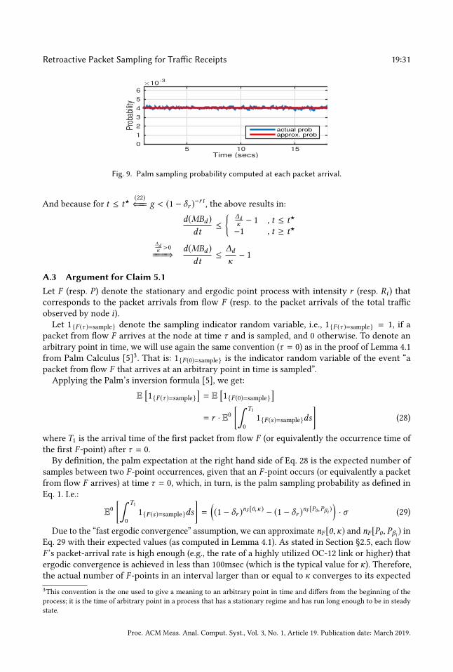
Retroactive Packet Sampling for Traffic Receipts 19:31
Time (secs)5 10 15
Pro
babi
lity
×10-3
0
1
2
3
4
5
6
actual probapprox. prob
Fig. 9. Palm sampling probability computed at each packet arrival.
And because for t ≤ t⋆(22)⇐== g < (1 − δr )−r t
, the above results in:
d(MBd )dt
≤
{ ∆dκ − 1 , t ≤ t⋆
−1 , t ≥ t⋆
∆dκ >0====⇒
d(MBd )dt
≤∆d
κ− 1
A.3 Argument for Claim 5.1Let F (resp. P ) denote the stationary and ergodic point process with intensity r (resp. Ri ) thatcorresponds to the packet arrivals from flow F (resp. to the packet arrivals of the total traffic
observed by node i).Let 1{F (τ )=sample} denote the sampling indicator random variable, i.e., 1{F (τ )=sample} = 1, if a
packet from flow F arrives at the node at time τ and is sampled, and 0 otherwise. To denote an
arbitrary point in time, we will use again the same convention (τ = 0) as in the proof of Lemma 4.1
from Palm Calculus [5]3. That is: 1{F (0)=sample} is the indicator random variable of the event “a
packet from flow F that arrives at an arbitrary point in time is sampled”.
Applying the Palm’s inversion formula [5], we get:
E[1{F (τ )=sample}
]= E
[1{F (0)=sample}
]= r · E0
[∫ T1
0
1{F (s)=sample}ds
](28)
where T1 is the arrival time of the first packet from flow F (or equivalently the occurrence time of
the first F -point) after τ = 0.
By definition, the palm expectation at the right hand side of Eq. 28 is the expected number of
samples between two F -point occurrences, given that an F -point occurs (or equivalently a packet
from flow F arrives) at time τ = 0, which, in turn, is the palm sampling probability as defined in
Eq. 1. I.e.:
E0[∫ T1
0
1{F (s)=sample}ds
]=((1 − δr )
nF [0,κ) − (1 − δr )nF [P0,Pβi )
)· σ (29)
Due to the “fast ergodic convergence” assumption, we can approximate nF [0,κ) and nF [P0, Pβi ) in
Eq. 29 with their expected values (as computed in Lemma 4.1). As stated in Section §2.5, each flow
F ’s packet-arrival rate is high enough (e.g., the rate of a highly utilized OC-12 link or higher) that
ergodic convergence is achieved in less than 100msec (which is the typical value for κ). Therefore,the actual number of F -points in an interval larger than or equal to κ converges to its expected
3This convention is the one used to give a meaning to an arbitrary point in time and differs from the beginning of the
process; it is the time of arbitrary point in a process that has a stationary regime and has run long enough to be in steady
state.
Proc. ACM Meas. Anal. Comput. Syst., Vol. 3, No. 1, Article 19. Publication date: March 2019.
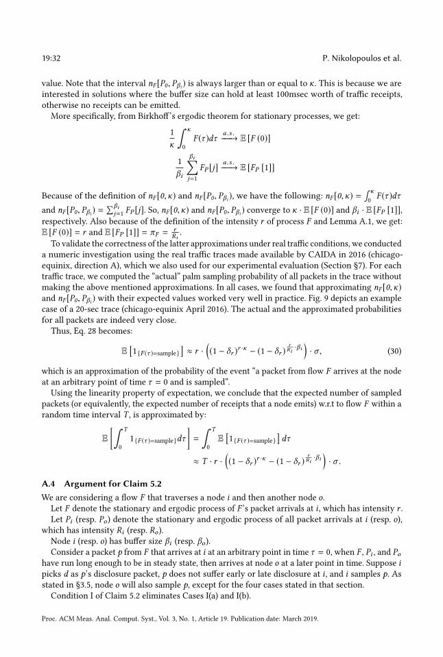
19:32 P. Nikolopoulos et al.
value. Note that the interval nF [P0, Pβi ) is always larger than or equal to κ. This is because we areinterested in solutions where the buffer size can hold at least 100msec worth of traffic receipts,
otherwise no receipts can be emitted.
More specifically, from Birkhoff’s ergodic theorem for stationary processes, we get:
1
κ
∫ κ
0
F (τ )dτa .s .−−−→ E [F (0)]
1
βi
βi∑j=1
FP [j]a .s .−−−→ E [FP [1]]
Because of the definition of nF [0,κ) and nF [P0, Pβi ), we have the following: nF [0,κ) =∫ κ0F (τ )dτ
and nF [P0, Pβi ) =∑βi
j=1 FP [j]. So, nF [0,κ) and nF [P0, Pβi ) converge to κ · E [F (0)] and βi · E [FP [1]],respectively. Also because of the definition of the intensity r of process F and Lemma A.1, we get:
E [F (0)] = r and E [FP [1]] = πF =rRi.
To validate the correctness of the latter approximations under real traffic conditions, we conducted
a numeric investigation using the real traffic traces made available by CAIDA in 2016 (chicago-
equinix, direction A), which we also used for our experimental evaluation (Section §7). For each
traffic trace, we computed the “actual” palm sampling probability of all packets in the trace without
making the above mentioned approximations. In all cases, we found that approximating nF [0,κ)and nF [P0, Pβi ) with their expected values worked very well in practice. Fig. 9 depicts an example
case of a 20-sec trace (chicago-equinix April 2016). The actual and the approximated probabilities
for all packets are indeed very close.
Thus, Eq. 28 becomes:
E[1{F (τ )=sample}
]≈ r ·
((1 − δr )
r ·κ − (1 − δr )rRi·βi)· σ , (30)
which is an approximation of the probability of the event “a packet from flow F arrives at the node
at an arbitrary point of time τ = 0 and is sampled”.
Using the linearity property of expectation, we conclude that the expected number of sampled
packets (or equivalently, the expected number of receipts that a node emits) w.r.t to flow F within a
random time interval T , is approximated by:
E
[∫ T
0
1{F (τ )=sample}dτ
]=
∫ T
0
E[1{F (τ )=sample}
]dτ
≈ T · r ·((1 − δr )
r ·κ − (1 − δr )rRi·βi)· σ .
A.4 Argument for Claim 5.2We are considering a flow F that traverses a node i and then another node o.
Let F denote the stationary and ergodic process of F ’s packet arrivals at i , which has intensity r .Let Pi (resp. Po ) denote the stationary and ergodic process of all packet arrivals at i (resp. o),
which has intensity Ri (resp. Ro ).Node i (resp. o) has buffer size βi (resp. βo ).Consider a packet p from F that arrives at i at an arbitrary point in time τ = 0, when F , Pi , and Po
have run long enough to be in steady state, then arrives at node o at a later point in time. Suppose ipicks d as p’s disclosure packet, p does not suffer early or late disclosure at i , and i samples p. Asstated in §3.5, node o will also sample p, except for the four cases stated in that section.
Condition I of Claim 5.2 eliminates Cases I(a) and I(b).
Proc. ACM Meas. Anal. Comput. Syst., Vol. 3, No. 1, Article 19. Publication date: March 2019.
Retroactive Packet Sampling for Traffic Receipts 19:33
Condition II eliminates Case II: Suppose d arrives at node i (resp. o) ∆i (resp. ∆o) time units after
p. Given that p does not suffer early disclosure at i , ∆i > κ. Given that the jitter between i and o isbelow µ, ∆o > ∆i − µ. Hence, according to Alg. 1 (lines 12,13), o samples p.
We now show that Condition III (βiRi=
βoRo=
βR ) and our “fast ergodic convergence” assumption
(§2.5) eliminate Case III:
Let nF [F0, Fd) denote the number of F -points between p’s and d’s arrivals.Let nPi [F0, Fd) denote the number of Pi -points between p’s and d’s arrivals at node i .Let nPo [F0, Fd) denote the number of Po-points between p’s and d’s arrivals at node o.Because of Eq. 12:
E[nPi [F0, Fd)
]=
Rir· nF [F0, Fd) .
E[nPo [F0, Fd)
]=
Ror· nF [F0, Fd) .
Because of the “fast ergodic convergence” assumption (§2.5) and Birkhoff’s ergodic theorem for
stationary processes, nPi [F0, Fd) and nPo [F0, Fd) converge to their expected value almost surely (a.s.).
The fact that i samples p implies that:
nPi [F0, Fd) ≤ βi .
Combining the above statements with Condition III (βiRi=
βoRo), we have:
nPi [F0, Fd) ≤ βia .s .===⇒ E
[nPi [F0, Fd)
]≤ βi
⇔Rir· nF [F0, Fd) ≤ βi
⇔Ror· nF [F0, Fd) ≤ βo
⇔ E[nPo [F0, Fd)
]≤ βo
a .s .===⇒ nPo [F0, Fd) ≤ βo .
This implies that p does not suffer late disclosure at o.
B OTHER MISBEHAVIORFake late disclosure. If domain x does not perform well w.r.t. flow F , x may try to prevent
the monitor from estimating x ’s performance w.r.t. F , by emitting fake late-disclosure warnings.
This does not help x , because a fake late-disclosure warning has the same effect as a fake-receipt
attack (§2.4): the best a domain can do is shift the blame for some loss/delay to one of its own
inter-domain links. For instance, suppose flow F crosses three subsequent nodes ix , ox (in domain
x), and iy (in domain y). Suppose ox emits a late-disclosure warning. As a result, for a short time
interval, the monitor cannot estimate the performance of the intra-domain segment {ix ,ox } orthe inter-domain link {ox , iy }. However, the monitor can still estimate the performance of the
segment {ix , iy }. Hence, ox ’s warning does not prevent the monitor from correctly estimating x ’sloss/delay, it only makes it unclear whether this loss/delay occurred on the intra-domain segment
or the inter-domain link adjacent to ox .Misconfiguration. We showed that a prioritization attack always harms the misbehaving
domain’s perceived delay performance, as long as κ and δr are set according to Claim 4.2. Domain
x may purposefully set κ and δr such that the conditions of Claim 4.2 do not hold. This does not
help x : Each participating node’s parameters must be set according to well-defined rules, which
Proc. ACM Meas. Anal. Comput. Syst., Vol. 3, No. 1, Article 19. Publication date: March 2019.
19:34 P. Nikolopoulos et al.
include honoring the inequalities of Claim 4.2 (§6.1); if a node’s parameters are set incorrectly, this
is apparent from the receipts it emits. For instance, a node’s quiet-period duration κ is apparent
to the monitor, because the node does not emit receipts during quiet periods; if a node uses a
shorter κ than it should, it will emit receipts when it should not (too close to the corresponding
disclosure packets), and the monitor will immediately detect that and ignore the node’s receipts.
Hence, emitting receipts produced with incorrect parameters is equivalent to emitting no receipts.
Forceful disclosure. A source that generates a flow F of packet rate r may purposefully craft
packets that will be picked as disclosure packets, in order to cause the nodes that observe F to
process it with a particular disclosure rate that is different from the proper disclosure rate δr setin each node according to Claim 4.2. The result is the same as if the nodes that observe F are
misconfigured, i.e., they have set δr incorrectly. However, it is important to note that this behavior
affects only the disclosure process for the particular flow F generated by the misbehaving source
(because one flow’s traffic cannot affect another flow’s disclosure process).
C SAMPLING INCONSISTENCYIn general, inconsistent sampling does not lead to incorrect performance estimates, because the
monitor detects the inconsistency and discards the corresponding samples. Inconsistent sampling
simply means that the monitor must wait longer to collect the minimum sample size necessary to
achieve the target accuracy, because some of the samples are discarded.
In §3.5, we stated all the cases where nodes may sample inconsistently. We can eliminate Case
III through proper parametrization (Claim 5.2, Condition III). We now discuss Cases I(a) and I(b)
(Case II is straightforward).
Consider a flow F that traverses nodes i and o.Case I(a): Consider a packet sequence {d0, . . . p, . . . d1, . . . d2} from F and suppose that d1 is
dropped between i and o; as a result, i picks d1 as p’s disclosure packet, whereas o picks d2 as p’sdisclosure packet, which may result in a different sampling outcome for p.
The monitor detects that nodes i and o picked different disclosure packets for p, because i emits
a receipt for d1 whereas o does not. To avoid drawing incorrect conclusions, the monitor does not
estimate the performance of the i-o segment with respect to F between packets d0 and d1.Case I(b): Consider a packet sequence {d1, p, . . . d2} from F and suppose that d1 is reordered
with p between i and o; as a result, node i picks d2 as p’s disclosure packet, whereas node o picks d1as p’s disclosure packet, which may result in a different sampling outcome for p.When there exists a reordering element between nodes i and o, there will be some packets
sampled by i and not by o, but also some packets sampled by o and not by i . The former could be
mistaken for loss between the two nodes, however, the latter indicates packet reordering between
them. Hence, the monitor does not estimate the performance of the i-o segment with respect to Fbetween packets d0 and d1. There exist more sophisticated ways to deal with packet reordering,
but we think that it does not make sense to complicate the mechanism given that, these days,
reordering events are the exception rather than the rule.
D COMPUTATIONSD.1 Minimum Sample SizeAs stated in §3.5, the monitor computes the minimum sample size Nγ ,ϵ necessary to achieve the
target (γ , ϵ)-accuracy using standard statistics. We now describe how.
Estimation of packet loss.
Proc. ACM Meas. Anal. Comput. Syst., Vol. 3, No. 1, Article 19. Publication date: March 2019.
Retroactive Packet Sampling for Traffic Receipts 19:35
In general, Nγ ,ϵ is a function of the target accuracy (ϵ and γ ) and some distribution moment of
the quantity we want to estimate (packet loss, in our case). Since we do not know in advance the
distribution of packet loss, we make one of two typical assumptions:
(1) Packet loss is a Bernoulli process: given the sequence of packets from flow F that arrive at
node i , any packet is lost before reaching node o with probability l ≥ lossmin, and packet-loss
events are independent. In this case, the standard central limit theorem (CLT) yields a closed
formula for Nγ ,ϵ :
Nγ ,ϵ =(ηϵ
)2
·1 − lossmin
lossmin, (31)
where η is the1+γ2-th quantile of the standard normal distribution.
(2) Packet loss is a bursty process governed by the Gilbert model [16]: it is either in a “low-loss”
(good) state or in a “high-loss” (bad) state, and it transitions between the two with given
probabilities. In this case, we approximate Nγ ,ϵ empirically through Monte-Carlo simulations.
We can choose one of these two assumptions based on the nature of the measured traffic (how bursty
we expect it to be). If we want to be conservative, we must choose (2), which yields a sufficient
sample size for both bursty and non-bursty traffic. The disadvantage is that, in the non-bursty
case, the resulting sample size will be larger than necessary, i.e., we will use more resources than
necessary to meet our target accuracy.
Estimation of delay quantiles.The minimum Nγ ,ϵ necessary to estimate the χ -quantile of the delay distribution with (γ , ϵ)-
accuracy is given by the theorem of the “γ -confidence interval for the sample median and other
quantiles” [5, 22]:
Nγ ,ϵ =(ηϵ
)2
·1 − χ
χ, (32)
where η is the1+γ2-th quantile of the standard normal distribution and 0 < χ < 1. Note that, in
the context of quantile estimation, the error ϵ is defined as the maximum difference, not between
the actual quantile and the estimated one—as one might expect—but between the index of the
actual quantile and the index of the estimated one at the order statistic. For example, suppose we
want to estimate the 75-th percentile of the delay distribution with (γ , ϵ)-accuracy, then Eq. 32
gives the necessary sample size Nγ ,ϵ , which guarantees that the actual delay quantile exists in the
interval between the (0.75 · (1 − ϵ) · N )-th and (0.75 · (1 + ϵ) · N )-th order statistics of the sample,
with probability γ . This is because of the normal approximation of the binomial distribution that is
proposed by the theorem for large sample sizes Nγ ,ϵ [5].
According to Equations 31 and 32, assuming lossmin ≪ 50%, the minimum sample size Nγ ,ϵnecessary for estimating the χ -quantile of the delay distribution for χ ≥ 50% is less than the
Nγ ,ϵ necessary for estimating packet loss with the same accuracy. Hence, we pick Nγ ,ϵ based on
Equation 31.
D.2 Minimum Buffer SizeAs stated in §6.1, we compute the minimum value of
βR for which both Inequalities 3 and 6 are
satisfied and set each node’s buffer size β accordingly. We now describe how.
Recall that, at this point, we have set all parameters except for the nodes’ buffer sizes and the
disclosure function r → δr .
Proc. ACM Meas. Anal. Comput. Syst., Vol. 3, No. 1, Article 19. Publication date: March 2019.
19:36 P. Nikolopoulos et al.
We start from Inequality 6 and solve forβR :
β
R≥
ln
((1 − δr )
rκ −Nγ ,ϵr ·T ·σ
)ln (1 − δr )
r . (33)
We want Inequality 33 to hold for any flow intensity r ∈ [rmin, rmax]. We observe that the term
on the right is a monotonically decreasing function of r . Hence, if we setβR such that the inequality
holds for r = rmin, it will hold for any r ∈ [rmin, rmax]:
β
R≥
ln
((1 − δr )
rminκ −Nγ ,ϵ
rmin ·T ·σ
)ln (1 − δr )
rmin. (34)
We want the minimum value ofβR for which both Inequality 3 and Inequality 34 hold:
• We constrain δr according to Inequality 3:
δr ∈(0, 1 − e−
1
rκ
).
• We observe that the term on the right of Inequality 34 is a convex function of δr . Hence, it is
minimized for some value of δr = δ ∗r ∈(0, 1 − e−
1
rκ
)that we compute numerically:
min
δr
{β
R
}=
ln
( (1 − δ ∗r
)rminκ −Nγ ,ϵ
rmin ·T ·σ
)ln (1 − δ ∗r )
rmin. (35)
Equation 35 gives the minimum value ofβR for which both Inequalities 3 and 6 hold. Hence, if a
node observes packet arrivals of maximum intensity R∗, we set its buffer size to
β∗ = R∗min
δr
{β
R
}.
So, in general, each node has a different buffer size, but the ratioβR is the same in all nodes. This
also means that the expected fraction of packets that suffer late disclosure is the same in all nodes.
Fig. 10 shows a node’s minimum buffer size in various realistic scenarios, as a function of the
minimum supported flow intensity rmin (10a), the measurement interval T (10b), and the minimum
loss rate lossmin (10c). For instance, assume rmin = 155K packets/sec, which corresponds to a
saturated OC-12 link assuming an average packet size = 500 bytes. Fig. 10b shows that a few MB of
memory are sufficient for measuring lossmin = 0.1% in T = 10 minutes. The plots were computed
assuming: κ = 100msec, ϵ = 10%, γ = 95%, R = 2.5Mpkts/sec (saturated OC-192 link assuming an
average packet size = 500 bytes), and a receipt size of 12 bytes.
We see that the buffer size drops rapidly as rmin, T , or lossmin increase, which makes sense: In
general, the larger a node’s buffer, the less often packets suffer late disclosure at the node, hence, the
more samples the node collects per time unit. Higher lossmin means that the monitor needs fewer
samples to reach a given target accuracy, hence each node needs to collect fewer samples per time
unit. Higher T means that the monitor is willing to wait longer to reach a given target accuracy,
hence, again, each node needs to collect fewer samples per time unit. Higher rmin means that we
are measuring bigger flows, which contribute more packets per time unit, hence the inter-arrival
time between disclosure packets is shorter for a given disclosure rate; as a result, each node needs
a smaller buffer to avoid late disclosure with a given probability and collect a given number of
samples per time unit.
Clarification: In Figs. 10b and 10c, we see that there always exists a minimum T and a minimum
lossmin at which β∗ becomes infinite, i.e., at these points, we could not achieve the target accuracy
Proc. ACM Meas. Anal. Comput. Syst., Vol. 3, No. 1, Article 19. Publication date: March 2019.
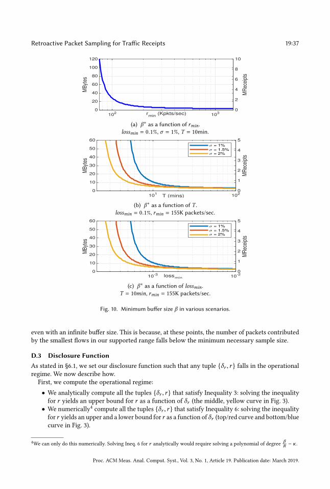
Retroactive Packet Sampling for Traffic Receipts 19:37
102
103
0
20
40
60
80
100
120
MB
ytes
rmin
(Kpkts/sec)0
2
4
6
8
10
MR
ecei
pts
(a) β∗ as a function of rmin.lossmin = 0.1%, σ = 1%, T = 10min.
101
102
0
10
20
30
40
50
60
MB
ytes
= 1% = 1.5% = 2%
T (mins)0
1
2
3
4
5
MR
ecei
pts
(b) β∗ as a function of T .lossmin = 0.1%, rmin = 155K packets/sec.
10-3
10-2
0
10
20
30
40
50
60
MB
ytes
= 1% = 1.5% = 2%
lossmin
0
1
2
3
4
5
MR
ecei
pts
(c) β∗ as a function of lossmin.T = 10min, rmin = 155K packets/sec.
Fig. 10. Minimum buffer size β in various scenarios.
even with an infinite buffer size. This is because, at these points, the number of packets contributed
by the smallest flows in our supported range falls below the minimum necessary sample size.
D.3 Disclosure FunctionAs stated in §6.1, we set our disclosure function such that any tuple {δr , r } falls in the operational
regime. We now describe how.
First, we compute the operational regime:
• We analytically compute all the tuples {δr , r } that satisfy Inequality 3: solving the inequality
for r yields an upper bound for r as a function of δr (the middle, yellow curve in Fig. 3).
• We numerically4compute all the tuples {δr , r } that satisfy Inequality 6: solving the inequality
for r yields an upper and a lower bound for r as a function of δr (top/red curve and bottom/blue
curve in Fig. 3).
4We can only do this numerically. Solving Ineq. 6 for r analytically would require solving a polynomial of degree
βR − κ .
Proc. ACM Meas. Anal. Comput. Syst., Vol. 3, No. 1, Article 19. Publication date: March 2019.
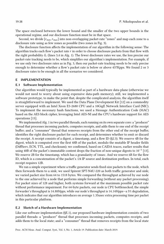
19:38 P. Nikolopoulos et al.
The space enclosed between the lower bound and the smaller of the two upper bounds is the
operational regime, and our disclosure function must be in that space.
Second, we divide [rmin, rmax] into non-overlapping packet-rate “zones” and map each zone to a
disclosure rate using as few zones as possible (two zones in Fig. 3).
The disclosure function affects the implementation of our algorithm in the following sense: The
algorithm tracks each flow’s packet rate r in order to choose disclosure packets from that flow with
the right probability δr (lines 3,4 in Alg. 1). The fewer disclosure rates we use, the less precise our
packet-rate tracking needs to be, which simplifies our algorithm’s implementation. For example, if
we use only two disclosure rates as in Fig. 3, then our packet-rate tracking needs to be only precise
enough to determine whether a flow’s packet rate is below or above 437Kpps. We found 2 or 3
disclosure rates to be enough in all the scenarios we considered.
E IMPLEMENTATIONE.1 Software ImplementationOur algorithm would typically be implemented as part of a hardware data-plane (otherwise we
would not need to worry about using expensive data-path memory); still, we implemented a
software prototype, to make the point that, despite the complicated analysis, the algorithm itself
is straightforward to implement. We used the Data Plane Development Kit [12] on a commodity
server equipped with an Intel Xeon E5-2680 CPU and a 10GigE Network Interface Card (NIC).
To implement the necessary hash functions, we used a Message Authentication Code (MAC)
based on the AES block cipher, leveraging Intel AES-NI and the CPU’s hardware support for AES
operations [15].
We implementedAlg. 1 in two parallel threads, each running on its own separate core: a “producer”
thread that processes incoming packets, computes receipts, and adds them to one end of the receipt
buffer; and a “consumer” thread that removes receipts from the other end of the receipt buffer,
identifies the right disclosure packet for each receipt, and determines whether to emit or discard
the receipt. A receipt consists of a digest, a timestamp, and a flow ID (§2.3). We reserve 4B for the
digest, which is computed over the first 48B of the packet, modulo the mutable IP header fields
(DiffServ, ECN, TTL, and checksum); we confirmed, based on CAIDA traces, earlier results that
using 48B of the packet’s immutable content drops the fraction of non-unique digests to 10−3
[13].
We reserve 2B for the timestamp, which has a granularity of 1msec. And we reserve 6B for the flow
ID, which is a concatenation of the packet’s /24 IP source and destination prefixes. In total, each
receipt requires 12B.
We ran a simple experiment where a traffic generator sends fixed-size packets to the node, which
then forwards them to a sink; we used Spirent SPT-N4U-220 as both traffic generator and sink;
we varied packet size from 64 to 1518 bytes. We compared the throughput achieved by our node
to the one achieved by a node that performs simple forwarding (without any packet processing).
For packet sizes of 128 and higher, both systems forward at the maximum possible packet rate
without performance impairment. For 64-byte packets, our node is CPU bottlenecked; the simple
forwarder’s throughput is 14.88Mpps, while our node’s throughput is 14.14Mpps—a 5% degradation,
which indicates that our algorithm introduces on average 1.35usec extra processing time per packet
in this particular platform.
E.2 Sketch of a Hardware ImplementationLike our software implementation (§E.1), our proposed hardware implementation consists of two
parallel threads: a “producer” thread that processes incoming packets, computes receipts, and
adds them to the local state; and a “consumer” thread that removes receipts from the local state
Proc. ACM Meas. Anal. Comput. Syst., Vol. 3, No. 1, Article 19. Publication date: March 2019.

Retroactive Packet Sampling for Traffic Receipts 19:39
and determines whether to emit or discard each receipt. The local state, however, is organized
differently: there is a receipt buffer for “normal” packets, stored in SRAM and accessible only as a
queue; and a receipt buffer for disclosure packets, stored in content-addressable memory (CAM)
that supports O(1) parallel lookups on the flowID field.
Organizing state in separate receipt buffers for normal and disclosure packets (as opposed to
a common receipt buffer) does not introduce any extra or any per-flow state; we keep exactly as
many receipts for normal and disclosure packets as Alg. 1, we just store them in two different kinds
of memory, because receipts for disclosure packets need to be looked up by flowID (hence require
CAM), whereas receipts for normal packets, which constitute the vast majority, do not (hence can
be stored in cheaper SRAM). For instance, consider the disclosure rates in the example of Fig. 3:
the higher of the two is 2.18 · 10−5%, which means that up to this fraction of observed packets are
picked as disclosure packets, whereas up to σ = 1% of observed packets in total are sampled. So,
if our analysis calls for a receipt buffer of 10.5MB (as in the particular example), about 0.23KB of
these need to be CAM, while the rest can be SRAM.
The consumer thread performs the actual sampling: It iterates over the receipt buffer for normal
packets, removes receipts, and performs the following operations for each receipt R that corresponds
to a normal packet p: (a) It retrieves the set of all receipts R in the disclosure buffer with the same
flowID as p. (b) It finds in R the receipt R′ that corresponds to p’s disclosure packet: it is the onewith the earliest timestamp that satisfies R′.time > R.time. It increments R′.packetCtr . It determines
whether to exclude or select p according to lines 10 and 12 of Alg. 1. (c) It checks whether disclosure
may have occurred late for p, i.e., if there is no receipt in R with time < R.time. If so, it emits a
warning.
The producer thread creates the local state: It processes each incoming packet p, computes
a receipt R′ for it, extracts the flowID, retrieves F ’s packet rate, checks whether to pick p as a
disclosure packet according to line 4 of Alg. 1, and adds R′ to the appropriate receipt buffer.
Moreover, the producer thread tracks flow packet rates based on information that is piggy-backed
by the consumer thread on the disclosure receipts. We previously said that receipts consist of four
fields (§2.3); receipts for disclosure packets have two additional fields for packet-rate tracking,
packetRate and packetCtr . Consider a flow F and suppose the first disclosure packet d1 arrives attime t1; when the second disclosure packet d2 arrives at time t2, the producer thread retrieves d1’sreceipt R, estimates F ’s packet rate (as R.packetCtr divided by t2− t1), and stores the estimate in d2’sreceipt (in the packetRate field); when the third disclosure packet d3 arrives, the node repeats theprocess, computes a new packet-rate estimate, and stores it in d3’s receipt; and so on. The node may
compute a brand new estimate every time a disclosure packet arrives, or it may update the previous
estimate, akin to keeping a moving-average filter [17]; we choose the latter, because it ensures a
smooth variation of estimate without risking sharp increases in rare cases where disclosure packets
arrive very close to each other.
We do not need perfect packet-rate tracking: Suppose a flow’s real packet rate is r , while theestimated one is r̂ . If r and r̂ are in the same zone (map to the same disclosure rate), the disclosure
process works as intended; if they map to different disclosure rates, then, of course, it is possible
that the chosen disclosure rate is too high or too low for the real packet rate, and we miss the
desired accuracy until the estimate catches up with the real value. The fewer disclosure-rate values
we use, the less likely we are to hit this scenario, and this is why we designed our disclosure process
to operate with smallest number of disclosure-rate values.
With this design, each node performs per packet: two hash computations, a couple of timestamp
comparisons, a read and a write access to SRAM, and a parallel lookup and an update in the CAM.
Received August 2018; revised December 2018; accepted January 2019
Proc. ACM Meas. Anal. Comput. Syst., Vol. 3, No. 1, Article 19. Publication date: March 2019.