Reversible and Irreversible Expansion of Lithium-ion Batteries Under aWide Range of Stress Factors

Peyman Mohtat∗, Suhak Lee, Jason B. Siegel, Anna G. Stefanopoulou

Mechanical Engineering Department, The University of Michigan, Ann Arbor, Michigan 48109-2125, USA

Abstract

Lithium-ion batteries cell thickness changes as they degrade. These changes in thickness consist of a reversible

intercalation-induced expansion and an irreversible expansion. In this work, we study the cell expansion

evolution under variety of conditions such as temperature, charging rate, depth of discharge, and pressure.

A specialized fixture was used to keep the cells at a constant pressure during cycling, while measuring the

thickness change both within a cycle and the cumulative growth over many cycles. The changes in positive

and negative electrode capacity and stoichiometric range can be diagnosed from the evolution of the reversible

expansion. The changes in the reversible expansion if combined with the voltage, lead to a higher-confidence

estimation of cell health parameters important for lifetime prediction and adoptive battery management such

as asymmetric charge/discharge power limits. This study raises the importance of monitoring the expansion

for enabling advanced and more-informed health diagnostics of lithium-ion batteries.

1. Introduction

The degradation of the lithium-ion battery is the result of a number of mechanical and chemical mecha-

nisms [1]. Important types of degradation are parasitic reactions such as Solid Electrolyte Interphase (SEI)

growth, lithium plating, and particle cracking leading to capacity fade and impedance growth. To optimally

operate a battery in terms of power limits, cycle-life, and safety, active knowledge of the internal aging

status of individual electrodes is needed. In addition to the changes in the electrochemical response mea-

sured through the voltage, lithium-ion batteries have a mechanical response and exhibit changes in thickness

during cycling. This response has been observed and investigated using in-situ X-ray diffraction (XRD)

[2, 3] and neutron imaging techniques [4]. The mechanical response consists of a reversible expansion caused

by (de)intercalation of lithium during cycling [5] and irreversible expansion caused by growth of the SEI

layer, lithium plating [6], and gas generation [7]. Recently, the effects of mechanical conditions on aging

has attracted attention with the aim of understanding the cell deformation as a function of state of charge

(SOC) and state of health (SOH).

∗Corresponding authorEmail address: pmohtat@umich.edu (Peyman Mohtat)

1

It has been shown that the measurement of the mechanical response either as stress or strain can improve

the accuracy of SOC estimation [8], and can be used for estimating SOH defined as capacity fade [9, 10]. The

relationship between the evolution of capacity fade, cell thickness, and effects of the external pressure on the

aging and cell performance has been the subject of a number of studies [11–15]. A shared conclusion of these

studies is the importance of monitoring and ideally controlling the external pressure. This is particularly

important for automotive applications since battery packs are usually designed with several stacked cells,

which means that due to irreversible expansion, the pressure on the cells can increase significantly and

adversely impact the performance of the cells [16, 17]. The evolution of the irreversible expansion also shows

a strong dependency on the cycling conditions [18–20], further reinforcing the idea of the coupling between

electrochemical and mechanical aging processes.

The inclusion of mechanical measurements also shows a great potential with regard to development of

advanced diagnostic methods. For example, it has been shown that measuring the thickness changes with

laser scanning can be a powerful tool for detecting lithium plating [21] and local aging [22]. Although the

aforementioned methods are mostly limited to a laboratory setting, in [23] we have showed that the cell diag-

nostics can also benefit greatly by incorporating the measurement of the cell overall thickness changes. Using

a simple model of the reversible part of the expansion and a fundamental analysis, we have demonstrated

that the addition of expansion measurements improves the estimation confidence levels and can drastically

reduce the data requirement and diagnostic test time, which is crucial for automotive applications. It should

be pointed out that in terms of real world implementation of these methods, the instrumentation of large

battery packs with stress/strain sensors remains challenging. Nevertheless, utilization of thin-film displace-

ment sensors for pouch type cells [24] and strain gauges for cylindrical cells [25] have shown encouraging

results to overcome some of these challenges.

The focus of this paper is to systematically verify the capability of aging diagnostics using cell expansion

under variety of aging conditions. The data collection campaign covers various degradation stress factors

in order to inform, parameterize, and validate the diagnostic model. This data collection campaign, for the

first time documents the evolution of the electrical and mechanical characteristics of multiple cells under

variety of stress factors. The testing matrix covers a wide range of conditions from charge/discharge C-rates,

temperatures, depth of discharges, and applied pressures. It is important to note that we collect data using

specially designed fixtures that enables the simultaneous measurement of mechanical and electrical response

under constant pressure. This expands significantly the prior experimental campaigns, which often performed

in unconstrained [19, 26] or completely constrained conditions [11, 27], where the cells are clamped to a fixed

distance and the irreversible expansion leads to increased compression over life.

2. Experimental Method

To study the degradation under variety of conditions a number of identical pouch cells were manufactured

in one batch using the fabrication facility at the University of Michigan Battery Lab (UMBL). The production

2

_

“Reversible” expansion

“Irreversible” expansion

𝑡𝑡1

Pouch cellV

+

δ

(a) (b)

(c) (d)

reversible expansion

total expansion

𝑡𝑡2 𝑡𝑡1

𝑡𝑡1𝑡𝑡1

𝑡𝑡2

𝑡𝑡2

𝑡𝑡2

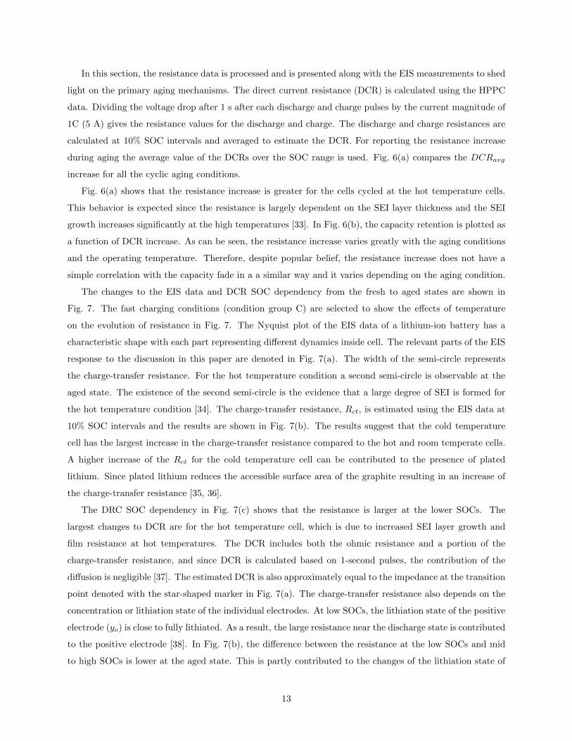
T

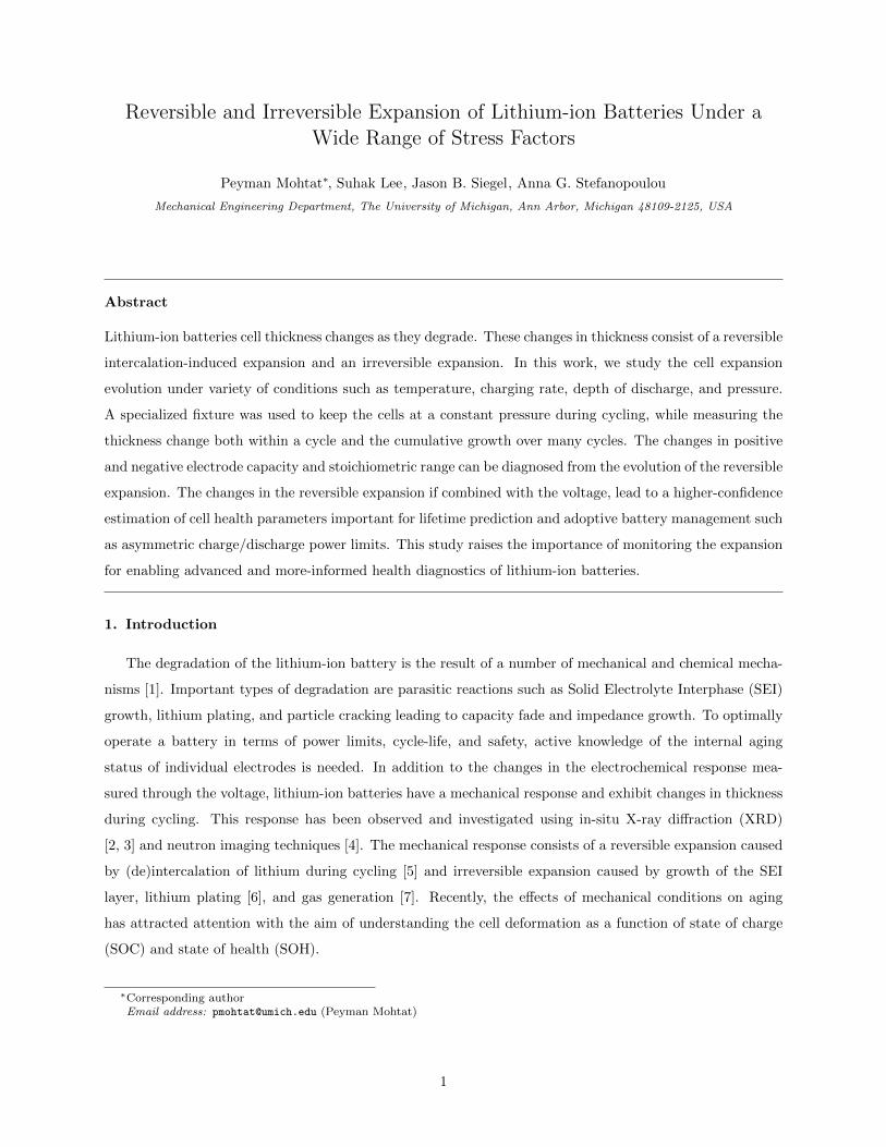
Figure 1: a) The fixture schematics, b) the testing configuration in the climate chamber, c) the current, voltage, and expansion

response for condition 2C @45◦C during cycling with the reversible and irreversible expansion. d) The voltage and expansion

response from two snapshots in time (t1,t2) plotted versus charge capacity. Note that the thickness change during one charge

cycle is shown as the total expansion and the relative change as the reversible expansion.

of the cells in one batch minimizes the cell-to-cell variation in performance that caused by manufacturing

process [28]. The cells were of graphite/NMC chemistry and designed as energy cells with the detailed

specifications shown in Table 1. Initial formation cycles were performed after the manufacturing to ensure

the safety and performance stability of the cells. Then the cells were assembled inside the fixture shown

in Fig. 1(a). The fixture was designed such that the top and bottom plates are fixed in place while the

middle plate is free moving. Compression springs were used to apply a prescribed pressure on the cell. The

important part is that the initial compression force and spring rate is such that the irreversible expansion

over life create a negligible increase in pressure. Initial target pressures of 5 PSI were achieved by adjusting

the spring compression to a fixed displacement using the threaded rods. Furthermore, polymer poron sheets

(Rogers, USA) were used on both sides of the pouch cell surface to achieve a more uniform pressure on the

cell and to avoid high pressure spots. The expansion was measured using a displacement sensor (Keyence,

Japan) mounted on the center of the top plate. The dynamic testing were carried using a battery cycler

(Biologic, France). The fixtures were installed inside a climate chamber (Cincinnati Ind., USA) in order

3

to control the temperature testing as shown in Fig. 1(b). The temperature was measured using a K-type

thermocouple (Omega, USA) place between the tabs on the surface of the battery.

The aging experiments were designed to cover an array of stress factors such as different C-rates during

charge and discharge, depth of discharges (DOD), temperatures, and applied pressures. Based on these stress

factors a number of testing conditions were selected that covers from low C-rate room temperature baseline

aging to high C-rate hot temperature accelerated aging. All the testing conditions are shown in Table 2.

Three different temperatures of hot (45◦C), cold (−5◦C), and room (25◦C) are considered for every aging

condition. The condition group G utilizes a realistic daily drive cycle with fast charging for an electric

vehicle. The details of the drive cycle are presented in Appendix C. The hot temperature/high C-rate

condition was selected as an accelerated aging test to study the effects of pressure on the cycle-life (shown

as condition group H).

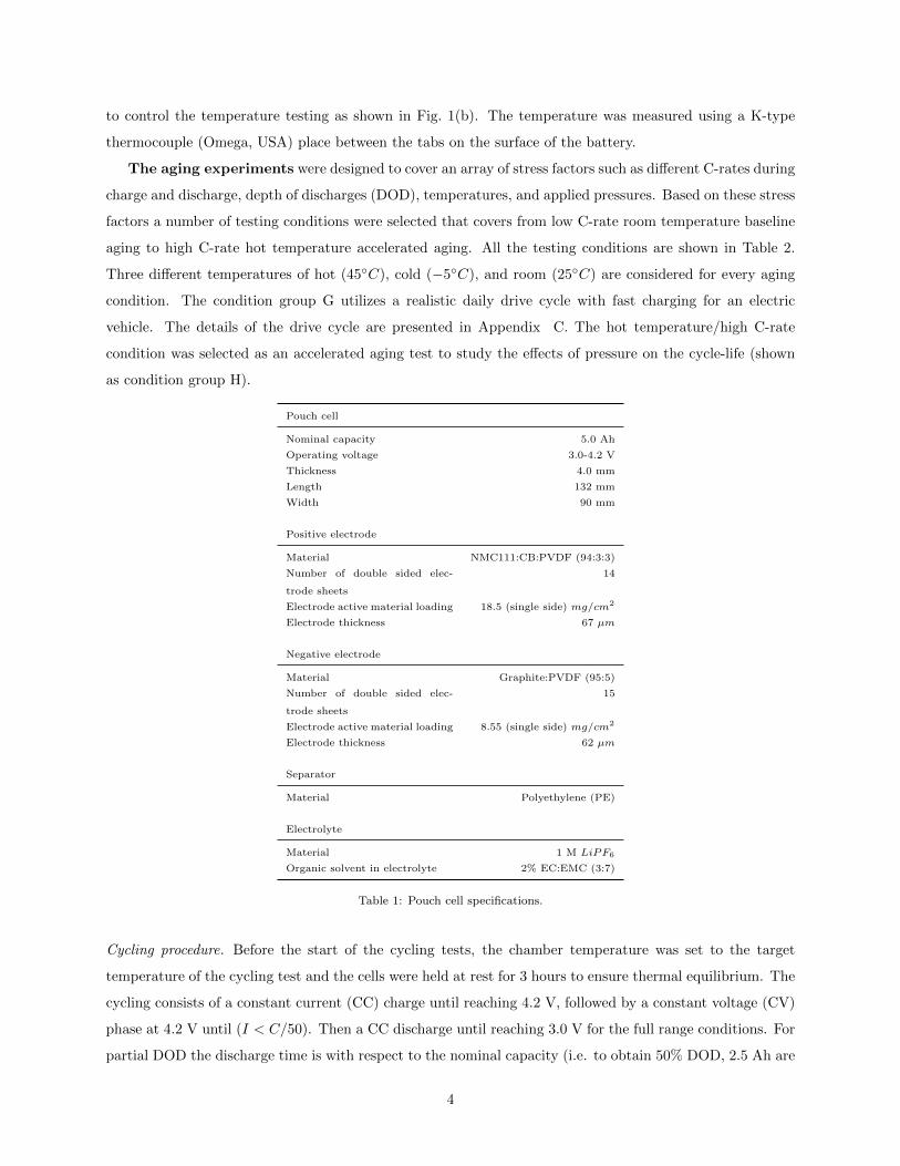
Pouch cell

Nominal capacity 5.0 Ah

Operating voltage 3.0-4.2 V

Thickness 4.0 mm

Length 132 mm

Width 90 mm

Positive electrode

Material NMC111:CB:PVDF (94:3:3)

Number of double sided elec-

trode sheets

14

Electrode active material loading 18.5 (single side) mg/cm2

Electrode thickness 67 µm

Negative electrode

Material Graphite:PVDF (95:5)

Number of double sided elec-

trode sheets

15

Electrode active material loading 8.55 (single side) mg/cm2

Electrode thickness 62 µm

Separator

Material Polyethylene (PE)

Electrolyte

Material 1 M LiPF6

Organic solvent in electrolyte 2% EC:EMC (3:7)

Table 1: Pouch cell specifications.

Cycling procedure. Before the start of the cycling tests, the chamber temperature was set to the target

temperature of the cycling test and the cells were held at rest for 3 hours to ensure thermal equilibrium. The

cycling consists of a constant current (CC) charge until reaching 4.2 V, followed by a constant voltage (CV)

phase at 4.2 V until (I < C/50). Then a CC discharge until reaching 3.0 V for the full range conditions. For

partial DOD the discharge time is with respect to the nominal capacity (i.e. to obtain 50% DOD, 2.5 Ah are

4

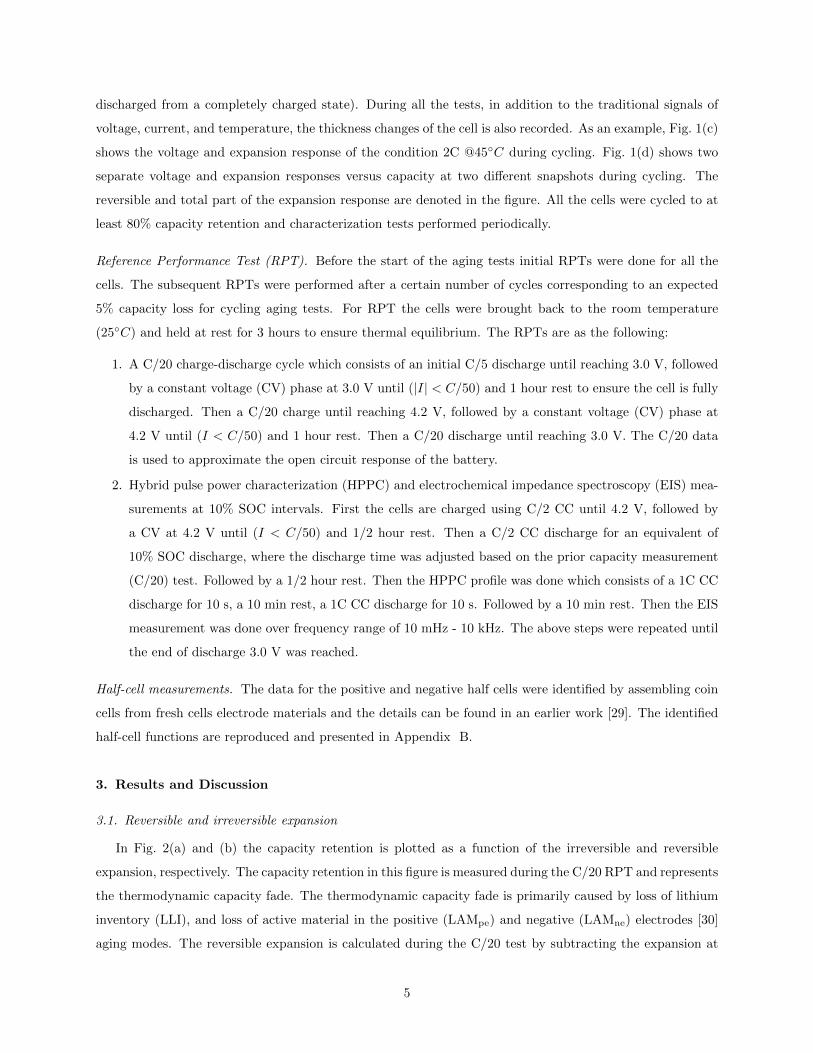
discharged from a completely charged state). During all the tests, in addition to the traditional signals of

voltage, current, and temperature, the thickness changes of the cell is also recorded. As an example, Fig. 1(c)

shows the voltage and expansion response of the condition 2C @45◦C during cycling. Fig. 1(d) shows two

separate voltage and expansion responses versus capacity at two different snapshots during cycling. The

reversible and total part of the expansion response are denoted in the figure. All the cells were cycled to at

least 80% capacity retention and characterization tests performed periodically.

Reference Performance Test (RPT). Before the start of the aging tests initial RPTs were done for all the

cells. The subsequent RPTs were performed after a certain number of cycles corresponding to an expected

5% capacity loss for cycling aging tests. For RPT the cells were brought back to the room temperature

(25◦C) and held at rest for 3 hours to ensure thermal equilibrium. The RPTs are as the following:

1. A C/20 charge-discharge cycle which consists of an initial C/5 discharge until reaching 3.0 V, followed

by a constant voltage (CV) phase at 3.0 V until (|I| < C/50) and 1 hour rest to ensure the cell is fully

discharged. Then a C/20 charge until reaching 4.2 V, followed by a constant voltage (CV) phase at

4.2 V until (I < C/50) and 1 hour rest. Then a C/20 discharge until reaching 3.0 V. The C/20 data

is used to approximate the open circuit response of the battery.

2. Hybrid pulse power characterization (HPPC) and electrochemical impedance spectroscopy (EIS) mea-

surements at 10% SOC intervals. First the cells are charged using C/2 CC until 4.2 V, followed by

a CV at 4.2 V until (I < C/50) and 1/2 hour rest. Then a C/2 CC discharge for an equivalent of

10% SOC discharge, where the discharge time was adjusted based on the prior capacity measurement

(C/20) test. Followed by a 1/2 hour rest. Then the HPPC profile was done which consists of a 1C CC

discharge for 10 s, a 10 min rest, a 1C CC discharge for 10 s. Followed by a 10 min rest. Then the EIS

measurement was done over frequency range of 10 mHz - 10 kHz. The above steps were repeated until

the end of discharge 3.0 V was reached.

Half-cell measurements. The data for the positive and negative half cells were identified by assembling coin

cells from fresh cells electrode materials and the details can be found in an earlier work [29]. The identified

half-cell functions are reproduced and presented in Appendix B.

3. Results and Discussion

3.1. Reversible and irreversible expansion

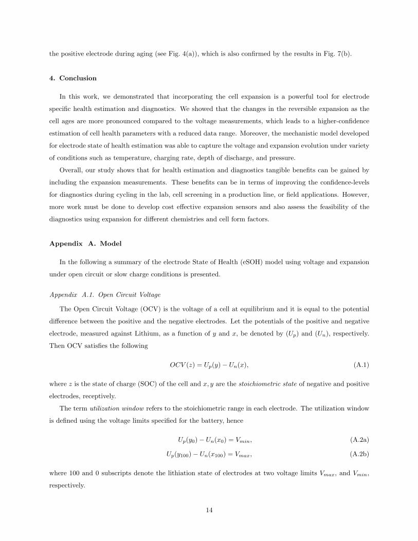
In Fig. 2(a) and (b) the capacity retention is plotted as a function of the irreversible and reversible

expansion, respectively. The capacity retention in this figure is measured during the C/20 RPT and represents

the thermodynamic capacity fade. The thermodynamic capacity fade is primarily caused by loss of lithium

inventory (LLI), and loss of active material in the positive (LAMpe) and negative (LAMne) electrodes [30]

aging modes. The reversible expansion is calculated during the C/20 test by subtracting the expansion at

5

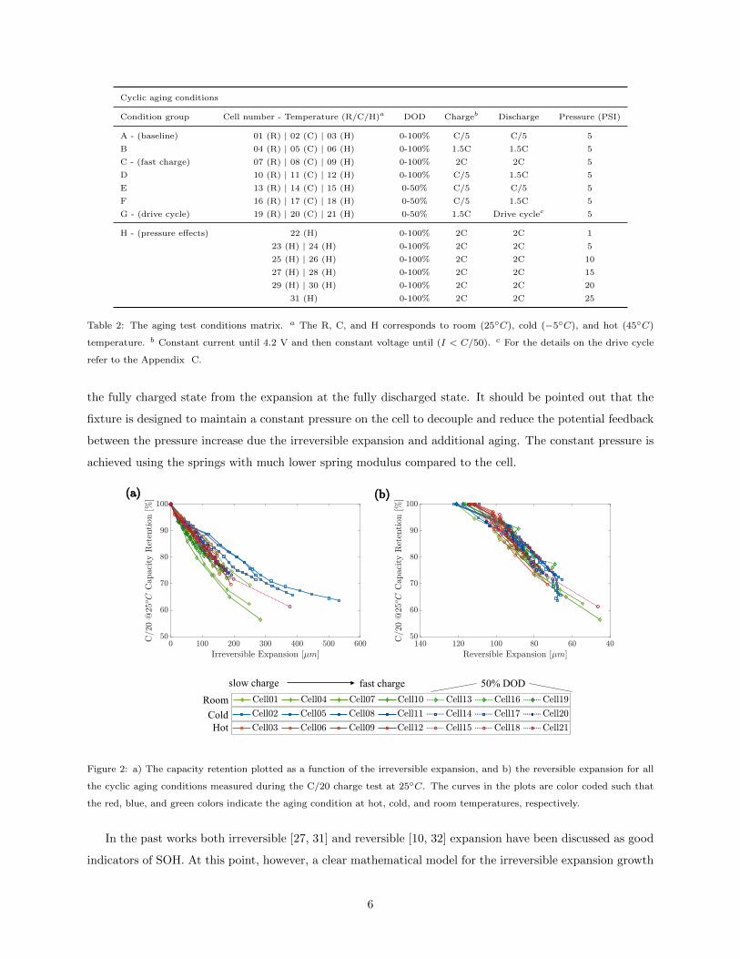
Cyclic aging conditions

Condition group Cell number - Temperature (R/C/H)a DOD Chargeb Discharge Pressure (PSI)

A - (baseline) 01 (R) | 02 (C) | 03 (H) 0-100% C/5 C/5 5

B 04 (R) | 05 (C) | 06 (H) 0-100% 1.5C 1.5C 5

C - (fast charge) 07 (R) | 08 (C) | 09 (H) 0-100% 2C 2C 5

D 10 (R) | 11 (C) | 12 (H) 0-100% C/5 1.5C 5

E 13 (R) | 14 (C) | 15 (H) 0-50% C/5 C/5 5

F 16 (R) | 17 (C) | 18 (H) 0-50% C/5 1.5C 5

G - (drive cycle) 19 (R) | 20 (C) | 21 (H) 0-50% 1.5C Drive cyclec 5

H - (pressure effects) 22 (H) 0-100% 2C 2C 1

23 (H) | 24 (H) 0-100% 2C 2C 5

25 (H) | 26 (H) 0-100% 2C 2C 10

27 (H) | 28 (H) 0-100% 2C 2C 15

29 (H) | 30 (H) 0-100% 2C 2C 20

31 (H) 0-100% 2C 2C 25

Table 2: The aging test conditions matrix. a The R, C, and H corresponds to room (25◦C), cold (−5◦C), and hot (45◦C)

temperature. b Constant current until 4.2 V and then constant voltage until (I < C/50). c For the details on the drive cycle

refer to the Appendix C.

the fully charged state from the expansion at the fully discharged state. It should be pointed out that the

fixture is designed to maintain a constant pressure on the cell to decouple and reduce the potential feedback

between the pressure increase due the irreversible expansion and additional aging. The constant pressure is

achieved using the springs with much lower spring modulus compared to the cell.

RoomColdHot

slow charge fast charge

(a) (b)

50% DOD

Figure 2: a) The capacity retention plotted as a function of the irreversible expansion, and b) the reversible expansion for all

the cyclic aging conditions measured during the C/20 charge test at 25◦C. The curves in the plots are color coded such that

the red, blue, and green colors indicate the aging condition at hot, cold, and room temperatures, respectively.

In the past works both irreversible [27, 31] and reversible [10, 32] expansion have been discussed as good

indicators of SOH. At this point, however, a clear mathematical model for the irreversible expansion growth

6

is not yet available for use in parametric identification. Moreover, Fig. 2(a) shows that the irreversible

expansion does not have a simple correlation with capacity fade and requires separate training for each aging

condition. On the contrary, the reversible expansion, has a well defined relationship to battery degradation

modes [23]. The reversible expansion has features that, similar to the voltage signal, are connected to the

phase transitions in the graphite. Additionally, the reversible expansion can be modeled with a relatively

simple approach that is introduced in Appendix A.

More importantly, Fig. 2(b) shows the strong and nearly linear correlation of the maximum reversible

expansion with capacity for all the aging conditions. Since the intercalation expansion of graphite is much

larger than the NMC [29], the reversible expansion response is largely a function of the graphite expansion.

Therefore, the strong correlation of the maximum reversible expansion with capacity is contributed to the

fact that LAMne at the negative electrode is the dominate aging mode. This statement is verified in the

following sections by estimating the electrode specific state of health (eSOH).

3.2. Mechanistic electrode model

In this section, we show the details of the parametric estimation for one case with a full charge and

discharge and also for reduced depth of discharge that is more expected in the field operation. It has been

shown that a higher confidence level in estimating the eSOH parameters is achievable with the inclusion

of expansion data [23]. Therefore, the advantages of the expansion is explored here by assuming a limited

availability of data. Here, for the analysis of the benefits of the expansion, cell 06 (1.5C/1.5C @45◦C) is

selected. It should be pointed out that the analysis was applied to all the other conditions, and there was

a similar results and conclusion. However, to avoid repetition and to keep the discussion more streamlined,

the aforementioned condition was selected to showcase the results of the analysis.

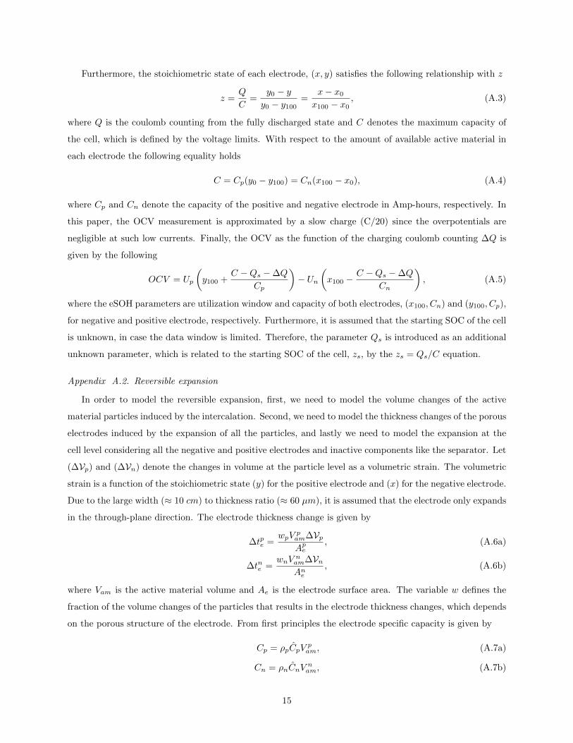
The voltage and expansion evolution of cell 06 measured during C/20 RPTs are shown in Fig. 3 (a) and

(b). The fitting results for voltage and expansion are also shown in Fig. 3 (a) and (b). It should be pointed

out that the model only requires the thickness change of the cell with respect to a thickness at the start of a

C/20 charge cycle, i.e. a partial or reduced data window of the reversible expansion. Furthermore, the cell

capacity and the initial SOC are also assumed to be unknown. For clarity of the presentation, the fitting

results are shown with the irreversible expansion added in Fig. 3 (b). As can be seen, the identified models

and the data are in good agreement at all the stages of aging. The fitted electrode parameters at every SOH

is also shown inside the Fig. 3 (a). The fitted model in Fig. 3 (a) and (b) is achieved by utilizing the full

data window (100-0% SOC) of both voltage and expansion. In Table 3, the estimated eSOH parameters

using the full data window for the fresh and the most aged state are shown. These identified parameters

are inferred to be the best estimated values since the full range of data is used for their estimation. For

the reduced data window (90-40% SOC), the estimation is repeated once using only voltage and second

time using voltage and expansion. The error percentage is calculated with respect to the full range values.

It should be noted that in all of the cases the estimation is done using a global search option, where the

optimization algorithm is done using a 100 randomly generated initial guesses within a predefined bound,

7

and the estimated parameters with the least value of the root mean squared error are selected as the answer

of the optimization. The upper bound for the C, Cn, and Cp parameters are set to the fresh cell values.

Aging state Data range Measurement typeEstimated parameters (error with respect to the full range values)

y0 Cp [Ah] x100 Cn [Ah] C [Ah]

Fresh Full Voltage+Expansion 0.88 5.80 0.82 6.02 4.97

76% aged Full Voltage+Expansion 0.73 5.48 0.84 4.52 3.84

76% aged ReducedaVoltage 0.79 (+8.0%) 5.36 (-2.2%) 0.80 (-5.3%) 5.13 (+13.3%) 4.12 (+7.4%)

Voltage+Expansion 0.74 (+1.0%) 5.32 (-2.8%) 0.85 (+1.5%) 4.44 (-2.0%) 3.82 (-0.5%)

Table 3: The results of estimation error analysis with a reduced data window, comparing the voltage only and voltage+expansion.

The analysis is done for the Cell 06 (1.5C/1.5C @45◦C). The error is calculated with respect to the aged values estimated

using the full range of voltage and expansion data. a The Reduced data window corresponds to 90-40% SOC.

(1.5C)(1.5C)|@ 45℃(a)

(b)

Capacity fade

Irreversible expansion

Reversible expansion

Figure 3: The results for the 1.5C @45◦C condition, a) the voltage response during the C/20 charge test @25◦C and the results

of model fitting, b) The expansion response during the C/20 charge test @25◦C and the results of model fitting. The lines are

color coded from green (fresh) to red (most aged).

From Table 3, comparing the estimation error of the voltage only and voltage plus expansion, it is evident

that estimation of negative electrode parameters, (x100, Cn), and the capacity, C, suffers greatly using only

the voltage. The estimation error is under 3% across the board for the expansion whereas for the voltage

the estimation error is as high 13%. This large error is particularly important for the capacity, which is

overestimated by 7.4%. As an example, for an electric vehicle with a 250 miles of range, the range would

8

be overestimated by about 20 miles. On the other hand, the expansion produces accurate estimates even

with a limited state of charge window, which enables fast and high-confidence diagnostics under limited

data window scenarios. Furthermore, the expansion can facilitate more frequent capacity estimation and

diagnostics for electric vehicles, where the state of charge window is often restricted and a deep depth of

discharge rarely happens.

The large estimation error of the voltage only measurements points to an underlying limitation. It has

been shown in [23] that the observability of the eSOH parameters is related to the rate changes of the half-cell

potential and expansion. The graphite has a very flat half-cell potential response in the high SOC region,

which makes the voltage measurement less sensitive to the lithiation changes in the graphite. The poor

observability of the graphite and NMC parameters is the direct consequence of the aforementioned behavior.

On the other hand, the rate change of half-cell expansion of graphite with respect to the lithiation is non-

zero, which makes the expansion measurement sensitive to the lithiation state of the graphite. Therefore, by

including the expansion data we are able to increase the observability of the graphite parameters and thus,

increase the estimation accuracy of the eSOH parameters.

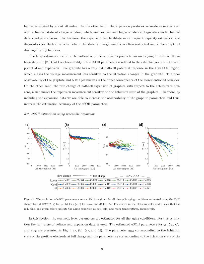
3.3. eSOH estimation using reversible expansion

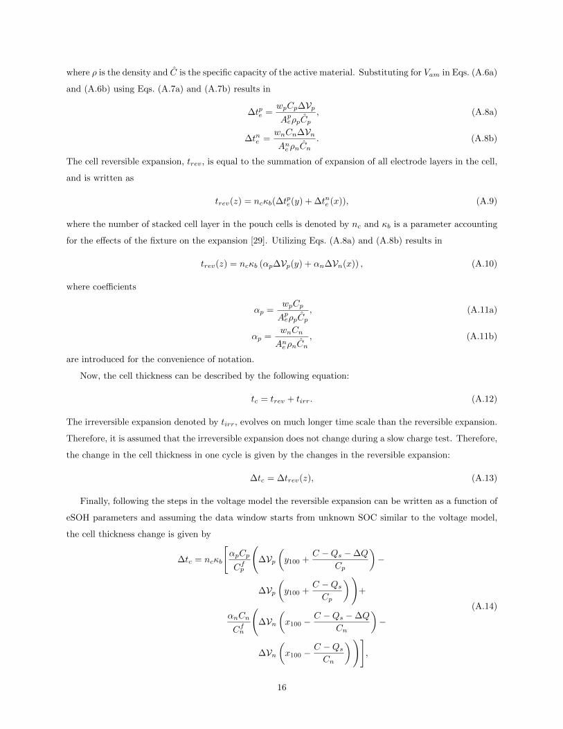
RoomColdHot

slow charge fast charge

(a) (b) (c) (d)

50% DOD

Figure 4: The evolution of eSOH parameters versus Ah throughput for all the cyclic aging conditions estimated using the C/20

charge test at @25◦C, a) for y0, b) for Cp, c) for x100, and d) for Cn. The curves in the plots are color coded such that the

red, blue, and green colors indicate the aging condition at hot, cold, and room temperatures, respectively.

In this section, the electrode level parameters are estimated for all the aging conditions. For this estima-

tion the full range of voltage and expansion data is used. The estimated eSOH parameters for y0, Cp, Cn,

and x100 are presented in Fig. 4(a), (b), (c), and (d). The parameter y100 corresponding to the lithiation

state of the positive electrode at full charge and the parameter x0 corresponding to the lithiation state of the

9

negative electrode at full discharge do not change significantly during aging. As a result, they are not shown

in Fig. 4. The parameters related to the cell structure and fixture configuration are presented in Appendix

D.

The maximum lithiation state of the positive electrode, y0, decreases considerably for all the aging

conditions in Fig. 4(a). These changes point to the fact that the Li inventory loss happens primarily during

charging with (SEI growth and lithium plating). Since the negative electrode quickly becomes the limiting

electrode during aging (Cn/Cp < 1), the lithium loss during charging leads to a shift (reduction) of y0

in the subsequent discharges. The shifts in the maximum lithiation state of the negative electrode, x100,

demonstrate an interesting response in Fig. 4(c). The balance between loss of lithium inventory and loss of

active material in the negative electrode governs the trajectory of x100. When LLI is the dominate aging

mode the x100 decreases and when the LAM is the dominate aging mode the x100 increases. In Fig. 4(c), for

the hot temperature cells the x100 reduces initially and then quickly increases. For the room temperature

cells the x100 is fairly unchanging overall, which points to a balance between LLI and LAM. For the cold

temperature cells the x100 decreases indicating that LLI is the main aging mode.

The loss of active material in the negative electrode (graphite) in Fig. 4(d) is significantly more than

the loss of active material in the positive electrode (NMC) in Fig. 4(b) for all the aging conditions. The

active material loss can occur with particle cracking, separation, and isolation [30]. Particle cracking exposes

fresh surface area to the electrolyte, which creates newly formed SEI layers. Therefore, a main reason for

the increase in SEI growth is due to the increase in particle cracking at the later stages of aging [27]. The

graphite is considered as a brittle material, which means that the increase and decrease of the internal

stresses during cycling can lead to growth of cracks, fatigue failure and ultimately material separation. High

charge-discharge rates also lead to a large stress gradient in the particles, which propagates the micro-crack

formations. The temperature rise is also greater at high C-rates compared to low C-rates conditions inducing

more SEI growth.

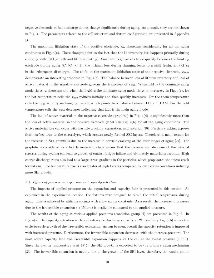
3.4. Effects of pressure on expansion and capacity retention

The impacts of applied pressure on the expansion and capacity fade is presented in this section. As

explained in the experimental section, the fixtures were designed to retain the initial set-pressure during

aging. This is achieved by utilizing springs with a low spring constants. As a result, the increase in pressure

due to the irreversible expansion (≈ 150µm) is negligible compared to the applied pressure.

The results of the aging at various applied pressures (condition group H) are presented in Fig. 5. In

Fig. 5(a), the capacity retention is the cycle-to-cycle discharge capacity at 2C, similarly Fig. 5(b) shows the

cycle-to-cycle growth of the irreversible expansion. As can be seen, overall the capacity retention is improved

with increased pressure. Furthermore, the irreversible expansion decreases with the increase pressure. The

most severe capacity fade and irreversible expansion happens for the cell at the lowest pressure (1 PSI).

Since the cycling temperature is at 45◦C, the SEI growth is expected to be the primary aging mechanism

[33]. The irreversible expansion is mainly due to the growth of the SEI layer, therefore, the results points

10

to the fact that an ample applied pressure can suppress the growth of the SEI layer [27]. Additionally, this

results reiterates the importance of applied pressure for the performance of lithium-ion cells and coupling

between the mechanical and electrochemical processes.

(a)

(b)

(c)

Higher pressure

Higher pressure

Higher pressure

Figure 5: a) The 2C capacity retention and b) the irreversible expansion for the condition group H; aging at different applied

pressures ranging from 1 to 25 PSI. c) The 2C capacity retention as a function of the reversible expansion. The measurements

are made during the continues cycling.

As mentioned before, for the NMC-graphite cells tested in this study, the LAM at the negative electrode

was the dominate aging mode (see Fig. 4(d)) under a variety of different aging conditions. Therefore, the

capacity of the cell is determined by the limiting electrode, which is the graphite. Moreover, the cell reversible

expansion response is also dominated by the graphite electrode, and the reduction of active material leads

to a lower reversible electrode expansion as well. Similar to the results in Fig. 2(b) the reversible expansion

11

has a linear relationship with the capacity retention for the different applied pressures shown in Fig. 5(c).

In summary, the rate of change in the reversible expansion with respect to capacity fade is similar for all

the applied pressures with higher pressures exhibiting a reduction of the maximum reversible expansion

magnitude due to the larger compression. Overall, this result shows that the relationship between the

reversible expansion and capacity fade holds for the cells cycled at different applied pressures as well.

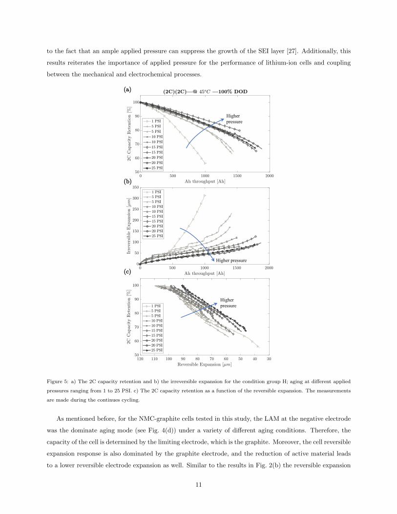
3.5. The resistance growth and EIS

(a)

RoomColdHot

slow charge fast charge

(b)

50% DOD

Figure 6: a) Direct current resistance (DCR) increase in percentage, averaged over the SOC range, versus Ah throughput for all

the cyclic aging conditions. b) The capacity fade plotted as a function of the DCR for all the cyclic aging conditions. The DCR

is calculated using the HPPC test. The curves in the plots are color coded such that the red, blue, and green colors indicate

the aging condition at hot, cold, and room temperatures, respectively.

𝑅𝑅𝑐𝑐𝑐𝑐

𝑅𝑅𝑆𝑆𝑆𝑆𝑆𝑆

𝑅𝑅𝑐𝑐𝑐𝑐

(a) (b) (c)

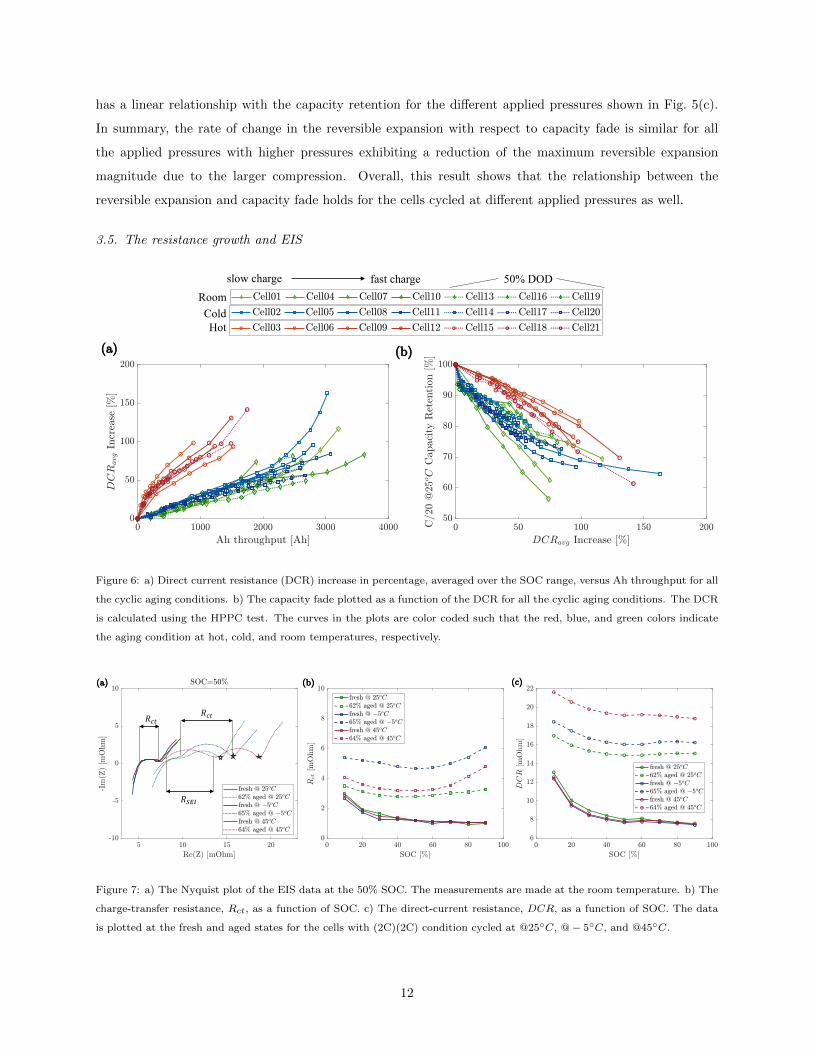
Figure 7: a) The Nyquist plot of the EIS data at the 50% SOC. The measurements are made at the room temperature. b) The

charge-transfer resistance, Rct, as a function of SOC. c) The direct-current resistance, DCR, as a function of SOC. The data

is plotted at the fresh and aged states for the cells with (2C)(2C) condition cycled at @25◦C, @ − 5◦C, and @45◦C.

12

In this section, the resistance data is processed and is presented along with the EIS measurements to shed

light on the primary aging mechanisms. The direct current resistance (DCR) is calculated using the HPPC

data. Dividing the voltage drop after 1 s after each discharge and charge pulses by the current magnitude of

1C (5 A) gives the resistance values for the discharge and charge. The discharge and charge resistances are

calculated at 10% SOC intervals and averaged to estimate the DCR. For reporting the resistance increase

during aging the average value of the DCRs over the SOC range is used. Fig. 6(a) compares the DCRavg

increase for all the cyclic aging conditions.

Fig. 6(a) shows that the resistance increase is greater for the cells cycled at the hot temperature cells.

This behavior is expected since the resistance is largely dependent on the SEI layer thickness and the SEI

growth increases significantly at the high temperatures [33]. In Fig. 6(b), the capacity retention is plotted as

a function of DCR increase. As can be seen, the resistance increase varies greatly with the aging conditions

and the operating temperature. Therefore, despite popular belief, the resistance increase does not have a

simple correlation with the capacity fade in a a similar way and it varies depending on the aging condition.

The changes to the EIS data and DCR SOC dependency from the fresh to aged states are shown in

Fig. 7. The fast charging conditions (condition group C) are selected to show the effects of temperature

on the evolution of resistance in Fig. 7. The Nyquist plot of the EIS data of a lithium-ion battery has a

characteristic shape with each part representing different dynamics inside cell. The relevant parts of the EIS

response to the discussion in this paper are denoted in Fig. 7(a). The width of the semi-circle represents

the charge-transfer resistance. For the hot temperature condition a second semi-circle is observable at the

aged state. The existence of the second semi-circle is the evidence that a large degree of SEI is formed for

the hot temperature condition [34]. The charge-transfer resistance, Rct, is estimated using the EIS data at

10% SOC intervals and the results are shown in Fig. 7(b). The results suggest that the cold temperature

cell has the largest increase in the charge-transfer resistance compared to the hot and room temperate cells.

A higher increase of the Rct for the cold temperature cell can be contributed to the presence of plated

lithium. Since plated lithium reduces the accessible surface area of the graphite resulting in an increase of

the charge-transfer resistance [35, 36].

The DRC SOC dependency in Fig. 7(c) shows that the resistance is larger at the lower SOCs. The

largest changes to DCR are for the hot temperature cell, which is due to increased SEI layer growth and

film resistance at hot temperatures. The DCR includes both the ohmic resistance and a portion of the

charge-transfer resistance, and since DCR is calculated based on 1-second pulses, the contribution of the

diffusion is negligible [37]. The estimated DCR is also approximately equal to the impedance at the transition

point denoted with the star-shaped marker in Fig. 7(a). The charge-transfer resistance also depends on the

concentration or lithiation state of the individual electrodes. At low SOCs, the lithiation state of the positive

electrode (yo) is close to fully lithiated. As a result, the large resistance near the discharge state is contributed

to the positive electrode [38]. In Fig. 7(b), the difference between the resistance at the low SOCs and mid

to high SOCs is lower at the aged state. This is partly contributed to the changes of the lithiation state of

13

the positive electrode during aging (see Fig. 4(a)), which is also confirmed by the results in Fig. 7(b).

4. Conclusion

In this work, we demonstrated that incorporating the cell expansion is a powerful tool for electrode

specific health estimation and diagnostics. We showed that the changes in the reversible expansion as the

cell ages are more pronounced compared to the voltage measurements, which leads to a higher-confidence

estimation of cell health parameters with a reduced data range. Moreover, the mechanistic model developed

for electrode state of health estimation was able to capture the voltage and expansion evolution under variety

of conditions such as temperature, charging rate, depth of discharge, and pressure.

Overall, our study shows that for health estimation and diagnostics tangible benefits can be gained by

including the expansion measurements. These benefits can be in terms of improving the confidence-levels

for diagnostics during cycling in the lab, cell screening in a production line, or field applications. However,

more work must be done to develop cost effective expansion sensors and also assess the feasibility of the

diagnostics using expansion for different chemistries and cell form factors.

Appendix A. Model

In the following a summary of the electrode State of Health (eSOH) model using voltage and expansion

under open circuit or slow charge conditions is presented.

Appendix A.1. Open Circuit Voltage

The Open Circuit Voltage (OCV) is the voltage of a cell at equilibrium and it is equal to the potential

difference between the positive and the negative electrodes. Let the potentials of the positive and negative

electrode, measured against Lithium, as a function of y and x, be denoted by (Up) and (Un), respectively.

Then OCV satisfies the following

OCV (z) = Up(y)− Un(x), (A.1)

where z is the state of charge (SOC) of the cell and x, y are the stoichiometric state of negative and positive

electrodes, receptively.

The term utilization window refers to the stoichiometric range in each electrode. The utilization window

is defined using the voltage limits specified for the battery, hence

Up(y0)− Un(x0) = Vmin, (A.2a)

Up(y100)− Un(x100) = Vmax, (A.2b)

where 100 and 0 subscripts denote the lithiation state of electrodes at two voltage limits Vmax, and Vmin,

respectively.

14

Furthermore, the stoichiometric state of each electrode, (x, y) satisfies the following relationship with z

z =Q

C=

y0 − yy0 − y100

=x− x0

x100 − x0, (A.3)

where Q is the coulomb counting from the fully discharged state and C denotes the maximum capacity of

the cell, which is defined by the voltage limits. With respect to the amount of available active material in

each electrode the following equality holds

C = Cp(y0 − y100) = Cn(x100 − x0), (A.4)

where Cp and Cn denote the capacity of the positive and negative electrode in Amp-hours, respectively. In

this paper, the OCV measurement is approximated by a slow charge (C/20) since the overpotentials are

negligible at such low currents. Finally, the OCV as the function of the charging coulomb counting ∆Q is

given by the following

OCV = Up

(y100 +

C −Qs −∆Q

Cp

)− Un

(x100 −

C −Qs −∆Q

Cn

), (A.5)

where the eSOH parameters are utilization window and capacity of both electrodes, (x100, Cn) and (y100, Cp),

for negative and positive electrode, respectively. Furthermore, it is assumed that the starting SOC of the cell

is unknown, in case the data window is limited. Therefore, the parameter Qs is introduced as an additional

unknown parameter, which is related to the starting SOC of the cell, zs, by the zs = Qs/C equation.

Appendix A.2. Reversible expansion

In order to model the reversible expansion, first, we need to model the volume changes of the active

material particles induced by the intercalation. Second, we need to model the thickness changes of the porous

electrodes induced by the expansion of all the particles, and lastly we need to model the expansion at the

cell level considering all the negative and positive electrodes and inactive components like the separator. Let

(∆Vp) and (∆Vn) denote the changes in volume at the particle level as a volumetric strain. The volumetric

strain is a function of the stoichiometric state (y) for the positive electrode and (x) for the negative electrode.

Due to the large width (≈ 10 cm) to thickness ratio (≈ 60 µm), it is assumed that the electrode only expands

in the through-plane direction. The electrode thickness change is given by

∆tpe =wpV

pam∆VpApe

, (A.6a)

∆tne =wnV

nam∆VnAne

, (A.6b)

where Vam is the active material volume and Ae is the electrode surface area. The variable w defines the

fraction of the volume changes of the particles that results in the electrode thickness changes, which depends

on the porous structure of the electrode. From first principles the electrode specific capacity is given by

Cp = ρpCpVpam, (A.7a)

Cn = ρnCnVnam, (A.7b)

15

where ρ is the density and C is the specific capacity of the active material. Substituting for Vam in Eqs. (A.6a)

and (A.6b) using Eqs. (A.7a) and (A.7b) results in

∆tpe =wpCp∆VpApeρpCp

, (A.8a)

∆tne =wnCn∆VnAne ρnCn

. (A.8b)

The cell reversible expansion, trev, is equal to the summation of expansion of all electrode layers in the cell,

and is written as

trev(z) = ncκb(∆tpe(y) + ∆tne (x)), (A.9)

where the number of stacked cell layer in the pouch cells is denoted by nc and κb is a parameter accounting

for the effects of the fixture on the expansion [29]. Utilizing Eqs. (A.8a) and (A.8b) results in

trev(z) = ncκb (αp∆Vp(y) + αn∆Vn(x)) , (A.10)

where coefficients

αp =wpCp

ApeρpCp, (A.11a)

αp =wnCn

Ane ρnCn, (A.11b)

are introduced for the convenience of notation.

Now, the cell thickness can be described by the following equation:

tc = trev + tirr. (A.12)

The irreversible expansion denoted by tirr, evolves on much longer time scale than the reversible expansion.

Therefore, it is assumed that the irreversible expansion does not change during a slow charge test. Therefore,

the change in the cell thickness in one cycle is given by the changes in the reversible expansion:

∆tc = ∆trev(z), (A.13)

Finally, following the steps in the voltage model the reversible expansion can be written as a function of

eSOH parameters and assuming the data window starts from unknown SOC similar to the voltage model,

the cell thickness change is given by

∆tc = ncκb

[αpCp

Cfp

(∆Vp

(y100 +

C −Qs −∆Q

Cp

)−

∆Vp(y100 +

C −QsCp

))+

αnCn

Cfn

(∆Vn

(x100 −

C −Qs −∆Q

Cn

)−

∆Vn(x100 −

C −QsCn

))],

(A.14)

16

where superscript (f ) denotes the initial or fresh value of the electrode capacity, furthermore, it is assumed

that the αn and αp coefficients only scale with the electrode capacity changes during aging.

Appendix A.3. Estimation Problem

For the reversible expansion model incorporation in the estimation problem, we need to identify the

(nc, κb, αn, αp) parameters. These parameters depend on the cell structure design as well as the fixture

configuration (i.e. applied pressure on the cell), and if we have information on them a rough estimate of the

parameters can be made for the purposes of eSOH estimation. However, in this paper, we propose a more

robust algorithm to calibrate these expansion related parameters. First, we introduce the voltage only eSOH

estimation problem, which is given by

minθ

N∑i=1

∥∥∥OCV (θ,∆Qi)− Vi∥∥∥2

subject to

Up(y100)− Un(x100) = Vmax,

Up

(y100 +

C

Cp

)− Un

(x100 −

C

Cn

)= Vmin.

(A.15)

where θ = [y100, Cp, x100, Cn, C,Qs] denotes the eSOH parameters. The OCV is given by Eq. (A.5), and the

constraints are the operating cell voltage limits defined by Eqs. (A.2a) and (A.2b). The measured voltage

at ∆Qi is denoted by Vi, which is ideally measured at open circuit condition or can be approximated using

a low charge rate (< C/5). Similarly, a second eSOH estimation problem is introduced, which utilizes the

simultaneous voltage and expansion measurements, and is defined by

minθ

N∑i=1

∥∥∥Y (θ,∆Qi)− Yi∥∥∥2

subject to

Up(y100)− Un(x100) = Vmax

Up

(y100 +

C

Cp

)− Un

(x100 −

C

Cn

)= Vmin

(A.16)

where Y (θ,∆Qi) = [OCV (θ,∆Qi),∆tc(θ,∆Qi)]T , vector of measurements is Yi = [Vi, δi]

T , and ∆tc is

given by Eq. (A.14). The last problem is for estimating the expansion related parameters given the eSOH

parameters, θ, and is defined by

minξ

N∑i=1

∥∥∥∆tc(ξ,∆Qi)− ˆδi

∥∥∥2

(A.17)

where ξ = [kb, αp, αn]. Note that, in the aforementioned parameter set kb = ncκb. Since in Eq. (A.14) the

(nc, κb) parameters appear only in a multiplicative form, these two parameters are not uniquely identifiable.

17

Appendix A.4. Estimation Procedure

The models presented so far can be used either during a slow charge or slow discharge. However, because

of the presence of hysteresis in voltage and expansion, different potential and expansion functions are needed

for charge and discharge. Since a large part of charging typically happens at a constant current, we also

carry out the estimation during charging. The functional forms for potential and expansion henceforth

correspond to the electrode response during cell charging. The functions are presented in Appendix B. The

estimation procedure for calibrating expansion parameters and estimating eSOH parameters using expansion

and voltage is as follows:

1. At the cell fresh state measure the voltage and expansion during a slow charge (C/20).

2. Estimate the eSOH parameter, θf , using Eq. (A.15) (voltage only) and the full range of data.

3. Estimate the expansion parameters, ξ, using Eq. (A.17) with the identified θf and the full range of

data.

4. At the cell aged state measure the voltage and expansion during a slow charge (C/20).

5. Estimate the eSOH parameter, θa, using Eq. (A.16) given the identified ξ.

Note that when using simultaneous expansion and voltage measurements, a full range of data is not neces-

sarily needed. In section 3.2, the estimation accuracy and error is compared for a case of full and limited

data window. For an in depth analysis of the data window requirements refer to the Ref. [23].

Appendix A.5. Quantifying the Aging Modes

The different aging mechanisms in the lithium-ion battery are divided into different modes of loss of

lithium inventory (LLI), loss of active material (LAMpe) of the positive electrode, and loss of active material

(LAMne) of the negative electrode [30]. In the following the superscripts (f ) and (a) denote the fresh and

aged states, respectively. The percentage amount of LAM in each electrode, is the reduction in available

individual electrode capacity (Cp, Cn) and it is given by

LAMpe% =

(1−

Cap

Cfp

)× 100, (A.18a)

LAMne% =

(1− Can

Cfn

)× 100. (A.18b)

The total loss of lithium denoted by LLI is defined as the percentage reduction of the amount of intercalated

lithium and is given by the following

LLI% =

(1− naLi

nfLi

)× 100, (A.19)

where the amount of intercalated lithium in the electrodes is given by

nLi =3600

F(y100Cp + x100Cn). (A.20)

18

Moreover, the cell traditional SOH (normalized capacity retention) is given by

SOH% =

(Ca

Cf

)× 100, (A.21)

where C is the maximum capacity of the cell using the slow charge/discharge test.

Appendix B. Half-cell charge functions

Up(y)[V ] = 4.3452− 1.6518y + 1.6225y2 − 2.0843y3

+ 3.5146y4 − 2.2166y5

− 0.5623e−4 exp(109.451y − 100.006)

Un(x)[V ] = 0.063 + 0.8 exp(−75(x+ 0.001))

− 0.0120 tanh

(x− 0.127

0.016

)− 0.0118 tanh

(x− 0.155

0.016

)− 0.0035 tanh

(x− 0.220

0.020

)− 0.0095 tanh

(x− 0.190

0.013

)− 0.0145 tanh

(x− 0.490

0.020

)− 0.0800 tanh

(x− 1.030

0.055

)∆Vn(x)[−] = (x < 0.12)(0.2x)

+ (0.12 ≤ x < 0.18)(0.16x+ 5e−3)

+ (0.18 ≤ x < 0.24)(0.17x+ 3e−3)

+ (0.24 ≤ x < 0.50)(0.05x+ 0.03)

+ (0.50 ≤ x)(0.15x− 0.02)

∆Vp(y)[−] = −1.1e−2(1− y)

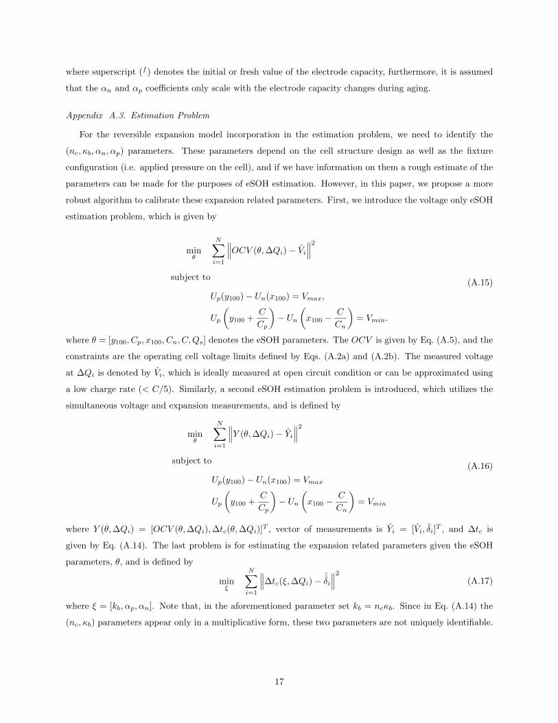
Appendix C. Drive cycle

A representative drive cycle for urban commute assuming a 33 kWh battery pack. The trip is composed

of several standard drive cycles based on a home-to-work/work-to-home (back and forth) commute scenario,

assuming a total of 71 miles of range. The standard drive cycles used for the synthetic drive cycle are

UDDS (Urban Dynamometer Driving Schedule), HWFET (Highway Fuel Economy Test), and US06 (one

of the Supplemental Federal Test Procedures). The depth of discharge is 50% assuming full charge is done

overnight.

19

Figure C.8: Current profile for the dynamic cycling.

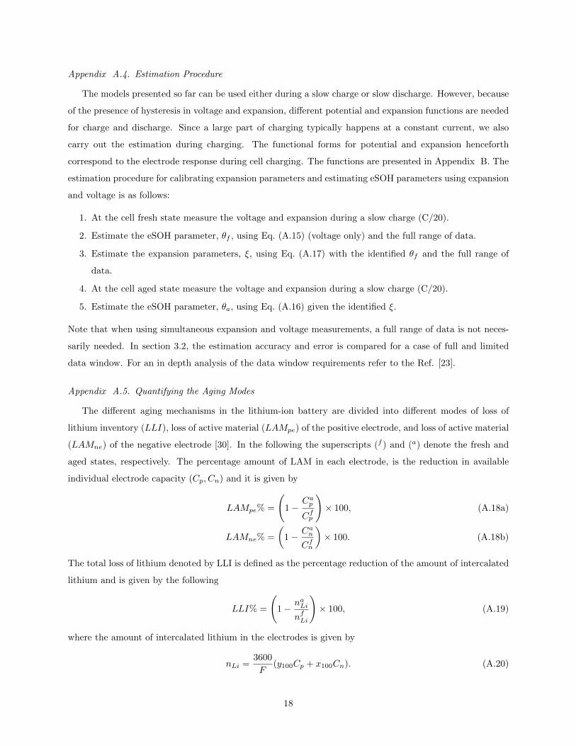
Pressure [PSI]Mean (standard deviation)

αp [µm] αn [µm] kb

5 80.27 (21.32) 45.60 (3.35) 29.87 (0.30)

Table D.4: The mean and standard deviation of the expansion parameters

Appendix D. Expansion parameters

Acknowledgment

The modeling work in this material was funded by the National Science Foundation under Grant No.

1762247. The experimental work in this material was thanks to the support of the Automotive Research

Center (ARC) in accordance with Cooperative Agreement W56HZV-14-2-0001 U.S. Army CCDC GVSC.

This work was performed in part at the University of Michigan Battery Lab, Energy Institute, and the

authors would like to thank Greg Less for his assistance on pouch cell fabrication. The authors would also

like to thank Yi Ding, and Matt Castanier of GVSC. Distribution A. Approved for public release; distribution

unlimited.

References

[1] J. Vetter, P. Novak, M. R. Wagner, C. Veit, K.-C. Moller, J. Besenhard, M. Winter, M. Wohlfahrt-

Mehrens, C. Vogler, and A. Hammouche, “Ageing mechanisms in lithium-ion batteries,” Journal of

power sources, vol. 147, no. 1-2, pp. 269–281, 2005.

[2] N. Zhang and H. Tang, “Dissecting anode swelling in commercial lithium-ion batteries,” Journal of

Power Sources, vol. 218, pp. 52–55, 2012.

[3] X. Yu, Z. Feng, Y. Ren, D. Henn, Z. Wu, K. An, B. Wu, C. Fau, C. Li, and S. J. Harris, “Simultaneous

operando measurements of the local temperature, state of charge, and strain inside a commercial lithium-

ion battery pouch cell,” Journal of The Electrochemical Society, vol. 165, no. 7, p. A1578, 2018.

20

[4] J. B. Siegel, A. G. Stefanopoulou, P. Hagans, Y. Ding, and D. Gorsich, “Expansion of lithium ion pouch

cell batteries: Observations from neutron imaging,” Journal of the Electrochemical Society, vol. 160,

no. 8, p. A1031, 2013.

[5] J. H. Lee, H. M. Lee, and S. Ahn, “Battery dimensional changes occurring during charge/discharge

cycles thin rectangular lithium ion and polymer cells,” Journal of power sources, vol. 119, pp. 833–837,

2003.

[6] V. A. Agubra, J. W. Fergus, R. Fu, and S.-Y. Choe, “Analysis of effects of the state of charge on the

formation and growth of the deposit layer on graphite electrode of pouch type lithium ion polymer

batteries,” Journal of power sources, vol. 270, pp. 213–220, 2014.

[7] B. Michalak, H. Sommer, D. Mannes, A. Kaestner, T. Brezesinski, and J. Janek, “Gas evolution in

operating lithium-ion batteries studied in situ by neutron imaging,” Scientific reports, vol. 5, p. 15627,

2015.

[8] S. Mohan, Y. Kim, J. B. Siegel, N. A. Samad, and A. G. Stefanopoulou, “A phenomenological model

of bulk force in a li-ion battery pack and its application to state of charge estimation,” Journal of the

Electrochemical Society, vol. 161, no. 14, p. A2222, 2014.

[9] J. Cannarella and C. B. Arnold, “State of health and charge measurements in lithium-ion batteries

using mechanical stress,” Journal of Power Sources, vol. 269, pp. 7–14, 2014.

[10] N. A. Samad, Y. Kim, J. B. Siegel, and A. G. Stefanopoulou, “Battery capacity fading estimation using

a force-based incremental capacity analysis,” Journal of The Electrochemical Society, vol. 163, no. 8,

p. A1584, 2016.

[11] J. Cannarella and C. B. Arnold, “Stress evolution and capacity fade in constrained lithium-ion pouch

cells,” Journal of Power Sources, vol. 245, pp. 745–751, 2014.

[12] A. Barai, R. Tangirala, K. Uddin, J. Chevalier, Y. Guo, A. McGordon, and P. Jennings, “The effect of

external compressive loads on the cycle lifetime of lithium-ion pouch cells,” Journal of Energy Storage,

vol. 13, pp. 211–219, 2017.

[13] A. S. Mussa, M. Klett, G. Lindbergh, and R. W. Lindstrom, “Effects of external pressure on the

performance and ageing of single-layer lithium-ion pouch cells,” Journal of Power Sources, vol. 385,

pp. 18–26, 2018.

[14] V. Muller, R.-G. Scurtu, M. Memm, M. A. Danzer, and M. Wohlfahrt-Mehrens, “Study of the influence

of mechanical pressure on the performance and aging of lithium-ion battery cells,” Journal of Power

Sources, vol. 440, p. 227148, 2019.

21

[15] L. Zhou, L. Xing, Y. Zheng, X. Lai, J. Su, C. Deng, and T. Sun, “A study of external surface pressure

effects on the properties for lithium-ion pouch cells,” International Journal of Energy Research, 2020.

[16] M. Wunsch, J. Kaufman, and D. U. Sauer, “Investigation of the influence of different bracing of au-

tomotive pouch cells on cyclic liefetime and impedance spectra,” Journal of Energy Storage, vol. 21,

pp. 149–155, 2019.

[17] T. Deich, S. L. Hahn, S. Both, K. P. Birke, and A. Bund, “Validation of an actively-controlled pneumatic

press to simulate automotive module stiffness for mechanically representative lithium-ion cell aging,”

Journal of Energy Storage, vol. 28, p. 101192, 2020.

[18] X. M. Liu and C. B. Arnold, “Effects of cycling ranges on stress and capacity fade in lithium-ion pouch

cells,” Journal of The Electrochemical Society, vol. 163, no. 13, p. A2501, 2016.

[19] R. Li, D. Ren, D. Guo, C. Xu, X. Fan, Z. Hou, L. Lu, X. Feng, X. Han, and M. Ouyang, “Volume

deformation of large-format lithium ion batteries under different degradation paths,” Journal of The

Electrochemical Society, vol. 166, no. 16, p. A4106, 2019.

[20] M. Lewerenz, C. Rahe, G. Fuchs, C. Endisch, and D. U. Sauer, “Evaluation of shallow cycling on two

types of uncompressed automotive li (ni1/3mn1/3co1/3) o2-graphite pouch cells,” Journal of Energy

Storage, vol. 30, p. 101529, 2020.

[21] C. Birkenmaier, B. Bitzer, M. Harzheim, A. Hintennach, and T. Schleid, “Lithium plating on graphite

negative electrodes: innovative qualitative and quantitative investigation methods,” Journal of The

Electrochemical Society, vol. 162, no. 14, p. A2646, 2015.

[22] J. Sturm, F. B. Spingler, B. Rieger, A. Rheinfeld, and A. Jossen, “Non-destructive detection of local

aging in lithium-ion pouch cells by multi-directional laser scanning,” Journal of The Electrochemical

Society, vol. 164, no. 7, p. A1342, 2017.

[23] P. Mohtat, S. Lee, J. B. Siegel, and A. G. Stefanopoulou, “Towards better estimability of electrode-

specific state of health: Decoding the cell expansion,” Journal of Power Sources, vol. 427, pp. 101–111,

2019.

[24] A. Knobloch, C. Kapusta, J. Karp, Y. Plotnikov, J. B. Siegel, and A. G. Stefanopoulou, “Fabrication

of multimeasurand sensor for monitoring of a li-ion battery,” Journal of Electronic Packaging, vol. 140,

no. 3, 2018.

[25] L. K. Willenberg, P. Dechent, G. Fuchs, D. U. Sauer, and E. Figgemeier, “High-precision monitoring

of volume change of commercial lithium-ion batteries by using strain gauges,” Sustainability, vol. 12,

no. 2, p. 557, 2020.

22

[26] P. Leung, C. Moreno, I. Masters, S. Hazra, B. Conde, M. Mohamed, R. Dashwood, and R. Bhagat,

“Real-time displacement and strain mappings of lithium-ion batteries using three-dimensional digital

image correlation,” Journal of Power Sources, vol. 271, pp. 82–86, 2014.

[27] A. Louli, L. Ellis, and J. Dahn, “Operando pressure measurements reveal solid electrolyte interphase

growth to rank li-ion cell performance,” Joule, vol. 3, no. 3, pp. 745–761, 2019.

[28] K. Rumpf, M. Naumann, and A. Jossen, “Experimental investigation of parametric cell-to-cell variation

and correlation based on 1100 commercial lithium-ion cells,” Journal of Energy Storage, vol. 14, pp. 224–

243, 2017.

[29] P. Mohtat, S. Lee, V. Sulzer, J. B. Siegel, and A. G. Stefanopoulou, “Differential expansion and voltage

model for li-ion batteries at practical charging rates,” Journal of The Electrochemical Society, vol. 167,

no. 11, p. 110561, 2020.

[30] C. R. Birkl, M. R. Roberts, E. McTurk, P. G. Bruce, and D. A. Howey, “Degradation diagnostics for

lithium ion cells,” Journal of Power Sources, vol. 341, pp. 373–386, 2017.

[31] G. Davies, K. W. Knehr, B. Van Tassell, T. Hodson, S. Biswas, A. G. Hsieh, and D. A. Steingart, “State

of charge and state of health estimation using electrochemical acoustic time of flight analysis,” Journal

of The Electrochemical Society, vol. 164, no. 12, p. A2746, 2017.

[32] Y. Kim, N. A. Samad, K. Y. Oh, J. B. Siegel, B. I. Epureanu, and A. G. Stefanopoulou, “Estimating

state-of-charge imbalance of batteries using force measurements,” in 2016 American Control Conference

(ACC), pp. 1500–1505, July 2016.

[33] M. Ecker, N. Nieto, S. Kabitz, J. Schmalstieg, H. Blanke, A. Warnecke, and D. U. Sauer, “Calendar and

cycle life study of li (nimnco) o2-based 18650 lithium-ion batteries,” Journal of Power Sources, vol. 248,

pp. 839–851, 2014.

[34] T. Momma, M. Matsunaga, D. Mukoyama, and T. Osaka, “Ac impedance analysis of lithium ion battery

under temperature control,” Journal of Power Sources, vol. 216, pp. 304–307, 2012.

[35] U. R. Koleti, T. Q. Dinh, and J. Marco, “A new on-line method for lithium plating detection in lithium-

ion batteries,” Journal of Power Sources, vol. 451, p. 227798, 2020.

[36] M. Petzl, M. Kasper, and M. A. Danzer, “Lithium plating in a commercial lithium-ion battery–a low-

temperature aging study,” Journal of Power Sources, vol. 275, pp. 799–807, 2015.

[37] A. Barai, K. Uddin, W. Widanage, A. McGordon, and P. Jennings, “A study of the influence of mea-

surement timescale on internal resistance characterisation methodologies for lithium-ion cells,” Scientific

reports, vol. 8, no. 1, pp. 1–13, 2018.

23

[38] S. J. An, J. Li, C. Daniel, S. Kalnaus, and D. L. Wood III, “Design and demonstration of three-electrode

pouch cells for lithium-ion batteries,” Journal of the Electrochemical Society, vol. 164, no. 7, p. A1755,

2017.

24