Revolution in Fertility, Schooling and Women’s Work, 1875-1940:Assessing Proposed Explanations

Matthias CINYABUGUMA, William LORD, and Christelle VIAUROUX∗

October 1, 2011

Abstract

The era between the Civil War and WWII was one of revolutionary change within the Americanfamily. Family size continued its long-term decline and by the 1930s fertility was not much abovecontemporary levels (later rising during the baby boom). The schooling of older children expandedtremendously, as epitomized by the ‘high school movement.’Additionally, the proportion of marriedfemales’adulthood devoted to market-oriented activities increased, even as market-oriented activityperformed at home declined. Horrific rates of infant and child mortality declined dramatically (withmore gradual gains since). Thus, this interval contained the emergence of many important featuresof contempoary families. This paper considers these trends jointly through calibration of succes-sive generations of representative husband and wife households who choose the quantity and qualityof children, household production, and the extent of mother’s involvement in market-oriented pro-duction. One important contribution is that standard explanations such as rising wages, decliningmortality, skill-biased technological change, curriculum improvements during the high school move-ment, reductions in morbidity, and reduced time costs of children cannot in combination reducefertility to observed levels or increase stocks of human capital to levels seen to be necessary by thecalibrations. Instead, a rising relative preference for child quality over quantity is also required,leading to an increased share of potential family income devoted to child education, child consump-tion and an increase in time mother’s investments in child quality. A second significant contributionis the gathering of information and strategies employed to present reasonable quantitative depictionsof the behavior of cohorts over an interval in which significant data limitations are pervasive.Keywords: American Family, Quantity-Quality Trade-Off, Convergence, High School Movement,

Married Female Labor Force Participation Rate.JEL classification numbers: I21, J13, J22, N31, and N32.

∗Matthias Cinyabuguma and Christelle Viauroux are assistant Professors of Economics at UMBC, and William Lordis Professor of Economics at UMBC. We are grateful to Marie Steele for wonderful-and cheerful-research assistance. Wealso thank Peter Rangazas and Marianne Wanamaker who usefully commented on an earlier draft of this paper.

0

1 Introduction

The era between the Civil War and WWII included many revolutionary changes in the American family,

as it obtained many of it’s contemporary features. Family size continued its long-term decline and by

the 1930s fertility was not much above current levels (later rising during the baby boom). The schooling

of older children expanded tremendously, as epitomized by the ‘high school movement.’ Although the

trend toward increased schooling expanded to encompass college for many in subsequent generations,

this earlier period firmly established the centrality of education to good employment. Additionally,

the proportion of married females’adulthood devoted to market-oriented activities increased, even as

market-oriented activity performed at home declined. Although those marrying in the mid-1920s still

typically quit work outside the home with a first birth, many returned in the 1940s after their children

had matured so that life-cycle rates of participation increased significantly. Even though the work-

family balance continued to shift powerfully toward work in subsequent decades, the earlier period

established that market work by married females was a serious and acceptable option. The Progressive

Era included the extension of the franchise to all female adults and, relatedly, the introduction of many

public health initiatives. Finally, horrific rates of infant and child mortality declined dramatically.

Although such mortality at the end of the period under consideration remained above current levels,

there was much higher confidence that a child born would not die during dependency.

This paper considers these trends jointly through calibration of successive generations of represen-

tative husband and wife households who choose the quantity and quality of their children, household

production, and the extent of mother’s involvement in market-oriented production. Exogenous rates of

infant and child mortality, returns to labor market experience, skill premiums, various costs of children,

and cohort income levels are model inputs used to generate time paths for schooling inputs, fertil-

ity, mother’s market work, and wages, including the gender wage ratio. These outputs enable us to

determine the fit of the model and assess proposed explanations of family change. One important con-

tribution is the finding that standard explanations such as rising wages, declining mortality, skill-biased

technological change, curriculum improvements during the high school movement, and reduced time

costs of children cannot in combination reduce fertility to observed levels or increase stocks of human

capital to levels seen to be necessary by the calibrations. Slower acquisition of human capital via work

experience over the period is (only) one reason the pace of the quantity-quality trade-off found in the

calibrations is below what is observed empirically.

For the calibrations to replicate observed behavior an increased ’taste’for child well-being is required.

This is modeled as a rising relative preference for child quality over quantity, an increased share of

potential family income devoted to child consumption, and an increase in time mothers invest in each

1

child’s quality. When calibrated under these assumptions the model fits the observed changes in the

family quite well. This increased taste for child well-being is consistent with increased bargaining

power for wives within marriage and a stronger relative preference for child quality among mothers

than fathers. A second significant contribution is the gathering of information and strategies employed

to present reasonable quantitative depictions of the behavior of cohorts over an interval in which

significant data limitations are pervasive.

The paper is organized as follows. Section II presents a brief description of the historical period,

the stylized facts to be explained, and those factors deemed to explain them. This is followed in

section III by a selective review of literature. Section IV presents the model. Section V explains the

calibration strategy. This is followed by a presentation of calibration results in section VI. A final

section summarizes and concludes.

2 The Historical Setting

The ‘second’ industrial revolution of the Post-Civil War decades involved the spread of large-scale

unskilled labor-saving capital equipment powered by, first steam, then electricity. These new machines

often substituted for human muscles (cf Galor and Weil (1996)), opening the door for more women

to be employed in manufacturing. The new machines also increased the demand for skilled blue-

collar workers to design and service machines. Large-batch and continuous process technologies led to

increases in the number of employees per firm, adding layers of bureaucracy which greatly increased

the need for clerical workers (cf. Goldin (1990)). Clerical employees needed more than rudimentary

reading, writing, and arithmetic skills; business skills such as an understanding of basic book keeping

and the ability to type were also increasingly necessary.

Acquisition of these skills required additional training, either on the job, in high school, or in business

schools. In the early transition this increase in demand was met by on—the-job training of high-skill blue

collar workers among men and learning-by-doing in manufacturing among females. Productivity would

be lower initially as employees had not yet learned how to perform the tasks required for job mastery.

Also, since the human capital acquired was firm or industry specific, workers presumably paid for at

least some portion of their training costs through lower wages. As they mastered their tasks, less output

was lost to learning and productivity was higher because of the additional experience-based skill. For

this reason, the returns to experience were quite high in the late nineteenth and early twentieth century.

Conversely, many jobs around 1900 required little schooling. Literacy was valued, but productivity in

handicrafts and manufacturing depended more on work experience than general school knowledge. A

few jobs required significant schooling (such as book keeper, clergy and school teacher), but for most

2

jobs literacy was suffi cient.

As skill-biased technical change proceeded, many of the prerequisites to performing advanced design

and mechanical engineering jobs could just as easily-and perhaps less expensively- be taught in school.

With no comparative advantage in the provision of this basic knowledge, firms began to require such

training before a man seeking a profession was hired. Similarly, with the expansion of clerical jobs,

females learned typing, stenography, and basics of book keeping in the classroom. The returns to

experience fell as draftsmen and machinists came to acquire their knowledge at school in ‘shop’courses,

while the return to education beyond literacy was increasing (the premium to ‘advanced,’or high school

training, remained high). Returns to experience have, however, recovered in the past few decades

(Olivetti (2006)).

Advances in transportation equipment and farm machinery increasingly allowed machines to sub-

stitute for human muscles, reducing the premium paid to strong males. Thus, over the first few decades

of the twentieth century, muscle power and work experience came to be less important determinants of

pay, while the contribution of schooling to earnings increased. These factors contributed to a narrowing

of the wage gap between men and women. The declining premium for muscles depressed men’s earnings

relative to women’s. Also, men in general had much more experience than women in the late nineteenth

century, so as the premium to experience fell, the impact was greater for men. Indeed, in 1890 the

vast majority of females ceased work upon marriage, so that the number of years of experience for

most females would be few. However, women born in the twentieth century devoted a larger portion

of their lives to market work, narrowing the experience gap. Indeed, Goldin (1986, 1990) and Goldin

and Polachek (1987) argue that higher average premiums for experience for females relative to males

accounts for close to 30 percent of the narrowing of the gender wage gap over the longer period from

1890 to 1970.

As the labor market adjusted to a higher demand for skilled workers, the premium paid to high school

graduates remained high or even increased. Before the high school movement, most high schools were

private and attended only by children of the affl uent. High schools were then most often preparatory

for college and learned professions, such as the clergy. Indeed, of those few high school graduates the

proportion who continued on to college in the late nineteenth century was perhaps 50%, a figure which

declined with the onset of the high school movement and would not be exceeded until the 1960s (even

as the proportion of successive birth cohorts attending college increased steadily (Goldin and Katz

(2008)). With the onset of the high school movement, a larger proportion of those students attending

high school viewed a diploma as a terminal degree. Schools responded to the different preparatory

needs of their students by dropping Latin from the curriculum and adding ‘shop’and typing courses.

3

An equally important change in the curriculum was the decline of the one-room schoolhouse which was

gradually supplanted by graded schools.

Through the first decade of the twentieth century high school attendance and graduation rates were

low and increasing only slowly. Low attendance meant the general populace was unwilling to publicly

support secondary schools. In turn, private tuition and room and board kept attendance from rising

high enough to encourage public support. Further, in the latter decades of the nineteenth century, a

family’s secondary earners were more often older children rather than wives. Especially in poor families,

children could not have been spared for higher education even if tuition was heavily subsidized.

After 1910, though, as incomes rose and population densities increased, public secondary education

began to spread widely. During the peak years of the ’high school movement’, between 1910 and 1940,

the high school graduation rate among youth rose from 9 percent to 50% (Goldin and Katz(2008, 195)).

Not only was the quantity of education received increasing, but so also was its quality as measured by

schooling expenditures. Real expenditures per youth aged 5-19 more than tripled between 1910 and

1950.

Goldin and Katz (2008) view the wage premium to skill as the outcome of a ‘race’between skill-

biased-technical change, which increases the demand for skilled labor, and increases in the supply of

skilled workers such as high school graduates. In the latter 19th century and into the 1910s the skill

premium remained high as increases in the supply and demand for skills were moderate and roughly

offsetting. The explosion in skilled workers with the high school movement, though, led to an appreciable

reduction in the premium to skills. Indeed, Goldin and Katz (2008, p. 316) find that "from 1910 to

1930 the skill premium fell by 1.28 percent per year on average."

The shift in total labor demand toward offi ce workers reduced the proportion of the workforce

for which large muscles were a big advantage, reducing the relative productivity and pay of males

(cf. Goldin and Polachek (1987)). Female clerical workers were more likely to return to work as

their children matured, so that the life cycle labor participation of married females increased as the

proportion of females working in clerical occupations soared. This helped produce the rise in the married

female labor force participation rate from 4.6 in 1890 to 21.6 in 1950 (Goldin (1990, p. 17, Table 2.1)).

The rise in schooling, lower premium to male strength, and increase in female market experience all

contributed to a narrowing of the gender wage gap. Goldin(1990) reports that between 1890 and the

1930s the gender wage gap in the economy as a whole closed from .46 to .56, narrowing only slightly

more to .60 by 1970.

Families were also becoming smaller as wives gave birth to fewer children . This trend was not new,

as fertility had been declining in the United States from at least the early nineteenth century. Jones and

4

Tertilt (2007) and Murphy, Simon and Tamura (2008) analyze historical cohort fertility in the United

States based on self reports of retrospective fertility of ever-married women coded in various Census

years. Women born in the 1850s who eventually married attained adulthood circa 1880 and would bear

about 5 children. Females born only a half century later, with fertility centered about 1930, end up

bearing only about 2.5 children, or roughly half that of their grandmothers.

There was a smaller decline in the number of children who would survive to adulthood than in

fertility, as deaths during infancy and childhood declined from horrific levels. Mortality was high and

variable in the United States until the last decades of the nineteenth century. High baseline mortal-

ity was spiked by periodic epidemics of cholera, typhoid, yellow fever, influenza and other infectious

diseases. However, in the 1870s or 1880s mortality began a rapid descent to much lower levels. The

white infant mortality rate, i.e., deaths in the first year of life per thousand live births—which was

staggering 214.8 in 1880—had declined to 120.1 in 1900 and to 26.8 by 1950 (Haines, 2000, Table 4.3);

these rates were appreciably higher for black children. Children who survived infancy were at lower,

but still significant, risk of death. Of 100 children born in 1880, an additional 12 died between the ages

of 1 and 15 (Murphy, Simon Tamura, 2008, Tables 14 and 15).

Preston and Haines (1991) describe how the mortality transition was facilitated by massive public

investments in clean drinking water and hygienic waste removal as well as advances in scientific under-

standing. Once the germ theory of disease gained acceptance, practices such as washing hands before

eating, quarantining those who are ill, boiling water, pasteurizing milk, and keeping living areas clean,

boosted health and reduced mortality. Many vaccines were introduced beginning in the latter nine-

teenth century, including cholera and typhoid, and for diphtheria, whooping cough, and tuberculosis

early in the twentieth century. The discoveries of sulfa drugs in the 1930s, then mass production of

penicillin in the 1940s, helped further reduce mortality and perhaps morbidity (Preston and Haines,

1991).

Mokyr (2000) argues that new understandings of the role of hygiene in preventing sickness and

death led mothers to devote more time to housework. Mothers, he argues, now believed that through

their efforts they could directly lower the probability of child death. Further, with the mechanisms of

disease still poorly understood, housewives made sure that any error in their effort would be on the

side of too much, rather than too little, cleanliness. Whereas God’s Will had previously been the sole

determinant of which children lived and died, now cleanliness had risen next to Godliness. Mothers’

obsession with cleanliness, he argues, delayed the onset of female market work.

More generally, this period was one of rising female power. The right of women to vote was

formalized by the 19th amendment to the United States Constitution in 1920. As described above,

5

more women were working for pay, and those who did earned an appreciably larger proportion of men’s

earnings than had been the case a generation before. Further, women spent less time debilitated in

pregnancy and were empowered to reduce the rate at which their children succumbed to illness.

3 Literature review

There is an immense literature on the topics of the high school movement, fertility decline, gender wage

gap, mortality decline, and role of women-including the rise in market work among married females,

for the United States. The following discussion is, of necessity, highly selective.

The scope, causes and implications of the high school movement are examined in depth by Goldin

and Katz (2008). They blend statistics on school enrollments and characteristics, and trends in wage

skill premiums, with deep appreciation of the interactions among technological change, institutions, and

returns to education. Skill-biased technological change increased the demand for skilled, well-educated

workers, while community characteristics (such as size of manufacturing base and homogeneity of

citizenry) help explain the timing, nationally and regionally, of the increases in education.

Since parents incur most costs of education, such as tuition and foregone earnings and housework of

children, while their children in adulthood reap the higher salaries education provides, most formulations

of schooling decisions assume parents are altruistic toward children (cf. Becker (1981)). That high

school attendance was low in the late nineteenth century, even though the increase in earnings from

high school was high, suggests some form of credit market imperfection (cf. Becker and Tomes (1986),

Galor and Ziera (2004)). Becker and Tomes point out that parents cannot legally assign debt to children.

This means that parental finance of children’s education reduces parental consumption. Consequently,

altruistic parents of limited means- relative to the cost of the fully effi cient level of child education- are

forced to make diffi cult trade-offs between own consumption and investments in child quality. When this

results in investments in children that are ineffi ciently low, parents are said to be ‘transfer-constrained’

(Lord (2002, Ch. 6). Among such parents, all intergenerational transfers motivated by altruism will

take the form of human capital bequests; financial transfers will be zero. Rangazas (2000) reports

simulations indicating that a macro growth model based on such transfer constraints performs much

better relative to observed growth characteristics of the U.S. than does a framework in which parents

always make the fully effi cient investments in their children. In the framework developed below we

follow the lead of this literature and limit transfers to children to human capital bequests.

Lord and Rangazas (2006) develop a model of the demographic transition and rise of schooling

investments since 1800. Their framework also assumes altruistic parents, while emphasizing the role of

declining wealth from family enterprise in reducing fertility. An important mechanism raising schooling

6

investments over time is that parental human capital is increasing relative to that of their still-dependent

children. This reduces the potential foregone earnings of children from school attendance relative to

family earnings. In this way the utility opportunity cost of schooling children declines. The framework

we develop highlights a similar mechanism.

Goldin and Katz (2008) argue that the returns to a year of education have varied not only over

time but also across education or skill levels at a point in time. They view these patterns as resulting

from interactions among the demand for and supply of skill, and institutions. Skill-biased technological

change (SBTC), which increases the demand for skilled or educated labor, accelerated in the latter

nineteenth century and then preceded at a fairly steady rate throughout the twentieth century. They

note that during the early acceleration, high school enrollments were low and the premium to skill was

bid up. As high school graduation rates soared after 1915 the premium to skill was bid down.

Goldin (1990) presents extensive evidence on the earnings of women relative to men, and why they

changed over time, across sectors and occupations. She finds that from 1890 to the 1930s there was a

significant narrowing of the gender wage gap. In Goldin and Polachek (1987) this narrowing is quan-

titatively partitioned into roles for changing amounts and returns to experience, increases in the level

and returns to education1, discrimination, and changing rewards to other gender characteristics (male

strength in particular). Increases in education are found to be most important, perhaps accounting for

more than 40 percent. Increases in the work experience of women relative to men are only somewhat

less important. Goldin (1990) and Goldin and Katz (2008) argue that changes in work responsibilities

along with a shift in training away from on-the-job and into schools reduced the returns to experience;

with a greater portion of work skills developed via high school attendance, there was less scope for

productivity advance from experience. For this reason, from 1890 to WWII the increase in total human

capital, obtained either on the job or at work, rises less rapidly than trends in the level and returns to

schooling alone (controlling for experience) would suggest.

Goldin (1990) chronicles the rise in female labor force participation, stressing important roles for

changes in the economy’s occupational distribution (especially the rise of the clerical sector), and for

institutions (marriage bars slowed the increase). Adeshade (2009) and Rotella (1980, 1981) envision

that an exogenous increase in high school attendance induced skill-biased technical change in offi ce

machines. Innovators foresaw that a large pool of educated females willing to work at wages below

males would complement skill-biased offi ce equipment. They responded to these incentives by designing

and manufacturing offi ce machinery, which increased the demand for female clerical workers, pulling

them from the home sector. Galor and Weil (1996) suppose that capital deepening accompanying the

1More generally, Goldin and Katz (2008) show the return to a year’s education varies both over time and across levelsof education. This is discussed further in the calibration section.

7

second industrial revolution decreased the return to strength, narrowing the gender wage gap, reducing

fertility and increasing married female labor force participation rates (MFLFPRs).

Other theories of the rise in MFLFPRs appeal to technological change in household production.

According to Greenwood, Seshadri and Yorukoglu (2005) the rise of labor-saving capital goods in the

household (clothes washers, dryers, vacuum cleaners, dishwashers, etc.), in combination with diminish-

ing marginal utility of non-tradeable goods produced in the household, reduced the marginal value of

females’time in the household sector. In their model, increases in the quantity and quality of durable

household appliances (which they model as declines in their price) reduce the reservation wages of

females, increasing MFLFPRs in the middle of the 20th century. In a theoretical calibration exercise

they find that half of the increase in MFLFPRs was due to labor-saving technology in the home. Bailey

and Collins (2010) confront the claims of Greenwood et al. with spatial data regarding the spread of

electricity and trends in fertility. They find little evidence to support the claims of Greenwood et al.

Albanesi and Olivetti (2007) argue that technological improvements related to the bearing and nursing

of children were instrumental to the rise in the labor force participation of mothers. Fernández, Fogli

and Olivetti (2004) propose a role for culture in the rise of MFLFPRs. They find that males whose

own mothers had worked are more likely to prefer a spouse who works. Mokyr (2000) argues that new

understandings of the role of hygiene in preventing sickness and death led late nineteenth and early

twentieth century mothers to devote more time to housework. Mothers, he argues, now believed that

through their efforts they could directly lower the probability of child death. Further, with the mech-

anisms of disease still poorly understood, housewives made sure that any error in their effort would

be on the side of too much, rather than too little, cleanliness. Mothers’obsession with cleanliness, he

argues, delayed the expansion of female market work. 2

Fertility in the U.S. fell through the 19th century until sometime in the 1930s, then rose during the

baby boom years, before falling to roughly replacement levels in recent decades. Jones and Tertilt (2007)

present time-series evidence on U.S. fertility and some of its correlates. They find a strong negative

2 In the context of economic development, Soares and Falcao (2008) consider linkages among adult longevity andMFLFP. In their framwork increases in adult life expectancy are the major driver of the rise in human capital, the declinein fertility and the movement of married women from the home to the market sector. They point out that increases in ownadult longevity lengthen the period over which investments in own market-oriented human capital can be recouped. Thisincreases human capital investments by females in their early adulthood, inducing them to substitute away from fertilityand increase market work. They also consider implications for investments in the human capital of children. To the extentthat the production of child quality utilizes mother’s time (and no goods), adult longevity has an ambiguous effect onchild quality: greater adult longevity for children increases the returns to their market human capital, but mother’s higherhuman capital increases the opportunity cost of investing in children. Hazan and Zobai (2006) examine effects on parentalhuman capital investments in children of perfectly foreseen increased longevity of children in adulthood. They point outthat when parents receive utility from the aggregate earnings of children in adulthood, increases in longevity increase thereturns to both quantity and quality. Consequently, increased longevity need not lead to fertility decline and increasededucation. However, Hazan (2009) shows that increased adult longevity in the United States over the period we considerwas associated with lower, rather than higher, life cycle market work among men. His finding limits the relevance of theSoares and Falcao mechanisms for the current study.

8

relationship between the occupational income of fathers and household fertility. A similarly strong

negative relationship is found between the education of the husband and/or wife and fertility. If there is

positive assortative spousal mating on education, all of these findings are consistent with Becker’s (1981)

observation that children require significant time, and that as the value of time (especially mother’s

wages) increases, children become more expensive. So long as children are treated symmetrically and

parents care about both the quantity and quality (i.e., earnings in adulthood) of children, higher

wages would reduces fertility and simultaneously induce a substitution toward child quality . Lord and

Rangazas (2006) simulate changes in the quantity and quality of children in the U.S. for the past two

centuries. They argue that an important determinant of the quantity-quality trade-off is the decline in

wealth from family businesses, which serves to reduce fertility.

Doepke (2005) examines implications of reductions in child mortality using several variants of the

Barro-Becker (1988) model of intergenerational altruism and endogenous fertility. He finds that in each

variant the number of children ever born declines, while the number of surviving children increases. His

results suggest that declining infant and child mortality cannot by themselves explain the large decline

in net reproduction rates observed in the United States (and other industrialized countries) over the last

century. Our results below are consistent with those models’predictions and we seek to identify which

other factors may explain declining fertility. Soares and Falcao (2008) briefly consider implications of

child mortality. Parents receive utility from surviving children and, as child mortality declines, so does

fertility. They note that lower child mortality increases the returns to parental investments in quality,

so that investments per child increase. In their framework the increase in parental investments per

child more than offsets the decline in fertility, so that total time investments in children increase. Thus,

lower child mortality reduces MFLFP.

Miller (2008) and Doepke and Tertilt (2011) review the rather conclusive evidence that women

place relatively more weight than men on child expenditures and welfare-what might be termed ’child

quality.’ Shifts in income from husbands to wives tend to reduce expenditures on alcohol, tobacco, and

men’s clothing while increasing expenditures on children’s’food and clothing. Evolutionary arguments

likewise suggest that men are relatively less concerned with quality of children than are women (cf.

Diamond (1997)). Miller (2008) points to the early twentieth century as a period in which female power

is rising, most spectacularly with passage of the 19th Amendment, ratified in 1920, granting women

the vote. Miller presents evidence that as individual states, and then the nation, ceded the franchise to

women, this engendered passage of legislation increasing local public health spending which, in turn,

contributed to the decline in infant and child mortality. Doepke and Tertilt (2009) suggest that greater

power for females can lead to more resources for schooling. They develop a framework in which men

9

granted the franchise to women in response to rising rates of return to human capital. These higher

returns meant that ceding power to females would increase the bargaining power of their daughters and

the education of their grandchildren. Cvereck (2007) argues that increased employment among single

females in the last decades of the nineteenth century increased their bargaining power within marriage.

The resulting increase in the share of marital output would rise as the gender wage gap narrows. Doepke

and Tertilit (2011) illustrate a noncooperative bargaining model in which a narrowing of the gender

wage gap can alter the mix of household public goods produced via household production functions.

In their framework, higher wages for wives make her time input more expensive and can reduce the

household supply of time-intensive public goods such as children even in the absence of a change in

preferences. Chiappori (1992) considers a cooperative marriage bargaining model. In his framework,

husbands and wives have different preferences for household public goods (such as quantity and quality

of children). As wive’s bargaining power increases, there is increased weight given to her preferences.

Collectively, this literature points to an increase in the relative power of females circa 1900 which led

to increased investment in the quality and well-being of children. Since greater investments per child

imply children who are more expensive, fertility may be expected to fall.

Our research builds on the foregoing research in a variety of ways. Below we present a model of two-

parent households in which fertility, child labor and human capital, and degree of married female labor

force participation are endogenous. This framework is calibrated to the United States between the Civil

War and WWII using a wide range of information, including changes in the gender wage gap, returns

to schooling, levels of human capital inputs, and infant and child mortality. The model’s flexibility and

careful calibration allow us to assess many of the explanations for family change considered above.

4 Modeling the household

4.1 Determinants of Human Capital

For each generation of adults there are four determinants of adult human capital; schooling, experience,

unskilled labor, and gender. The human capital of an adult male in period t is [h0mt + ht]Emt

while that of a female is [h0ft + ht]Eft. Here, ht is the number of units of schooling human capital

bequeathed by the parents of t − 1 to their children and is assumed to be equal across males and

females. h0ft(h0mt) is the stock of ‘unimproved’human capital associated with nature’s endowment,

learning by doing/observation prior to market work, and any minimum legal or cultural requirements

of parents regarding food, attention and training of their children. Thus, it is the ‘no-schooling’stock

of human capital. In general, the greater physical strength of males means that h0mt > h0ft, although

as argued by Galor and Weil (1996) the market premium to this strength differential has declined

10

over time.3 Emt(Eft) indicates how schooling and unskilled human capital are augmented by work

experience.

The potential earnings of males and females are determined by the market valuation of their stocks

of human capital. The market values units of unskilled human capital and units of skilled human

capital equally whether provided by males or females. That is, gender earnings differences depend

upon differences in the stocks of human capital by gender and differences in time worked in the market

rather than discrimination. It is standard to view each effi ciency unit of human capital as being valued

at some constant rate per unit, say wt. However, market conditions may lead to circumstances in which

higher and lower levels of human capital are valued differently. Goldin and Katz (2008) regard this as

an interaction between changes in the supply of skill by households and the demand for skill by firms.

To accommodate this possibility, units of unskilled human capital are paid at rate wt while units of

skilled or schooling human capital are rewarded at rate wt. In particular, when skill-biased technical

change (and thus firm demand for skill) proceeds more rapidly than skill supply, wt is increasing in the

stock of schooling capital. This is captured by

wt = wthεt.

Thus the potential earnings of a male are

(4.1.1) wth0mtEmt +(wth

εt

)htEmt = wt

[h0mt + h1+εt

]Emt = wthmt,

where hmt has scaled the schooling human capital by its market premium over unskilled human capital

so as to enable valuation of each unit by wt. Similarly, the potential adult female earnings are

(4.1.2) wt

[h0ft + h1+εt

]Eft = wthft.

Combining (4.1.1) and (4.1.2) yields the potential household earnings

wt(hft + hmt) = wtht.

If the ‘race’between skill and technology just offset one the other, ε = 0 and hmt and hft are simply

the (unscaled) human capital of males and females (while ht is the sum of adult human capital in the

household). The ratio of an adult female’s earnings working full-time to those of an adult male working

full-time is

γt =wthftwthmt

=hfthmt

,

Hence, the gender wage gap is

(4.1.3) 1− γt.3This could be modeled either as a reduction in the price of male unskilled human capital, or as done here, a reduction

in the units viewed by the market.

11

4.2 Production of Schooling Human Capital

Schooling human capital is acquired during dependency and deployed during adulthood. Parents of

generation t− 1 choose the quality of education, the goods inputs such as teachers and books, xt, the

quantity of their children’s education-fraction of youth devoted to schooling st. They also choose the

time spent on human-capital enhancing activities by mother et, the effectiveness of which depends on

the mother’s human capital hft. Thus, the schooling human capital produced, and which children can

deploy as adults in t+ 1 is given by

(4.2.1) ht+1 = bpt sθpst x

θpxt (hftet)

θphe ,

where bpt is an effi ciency scalar, and θps, θ

px, θ

phe ∈ (0, 1) are production function parameters (elasticities).

4.2.1 Preferences

Parents are assumed to care about the number of children surviving to adulthood nt+1 (half of whom

are boys), the earnings in adulthood of those children, and the consumption of household produced

goods. These sentiments are embodied in the utility function Ut for parents beginning adulthood in t

(4.2.2)

Ut = lnGt + ψt lnwt+1h1+εt+1 (Emt+1 + Eft+1)

nt+12

+ σt lnwt+1(h0ft+1 + h0mt+1)(Emt+1 + Eft+1)nt+1

2,

where Gt is the consumption of household production goods.

Potential earnings of children in adulthood derive from two sources. The third term is the earnings

across all surviving children derived from unschooled (or unskilled) human capital. Parent’s relative

taste for these ’unimproved’earnings is σt; such earnings may be increased by choosing to have a larger

number of surviving children nt+1. The aggregate earnings of adult children associated with schooling

human capital is given by the second term. The relative preference for such earnings is captured by

ψt , and these earnings may be increased by having more surviving children nt+1 and by investing

more in their education (which increases h1+εt+1 ). In the description of the budget set below, it is seen

that all surviving children impose costs, and that such costs are not a matter of choice. All surviving

children also confer ’nature’s bounty’of the unimproved human capital. Bequeathing schooling human

capital to children imposes additional costs, and these costs are only voluntarily undertaken.4 In

general, parents may place unequal valuations on earnings potential by source.5 Andreoni (1990) in an

influential paper argues that altruists get a ’warm glow’from their own contributions to a recipient,

4The costs of unimproved earnings may include some expenditures on mandatory schooling; the key feature is thatthese costs are not subject to choice.

5As noted in the literature review, there is evidence that men and women have different preferences over fertility andquality; this specification allows us to analyze implications of those differences.

12

and therefore place a different valuations on own contributions than to other sources (here unimproved

earnings from ’nature’) of a recipient’s well-being. Both ψt and σt embody a taste for quantity of

children. However, only ψt reflects a taste for improving the quality (i.e., schooling) of individual

children. For this reason an increase in ψt/σt is viewed as an increased relative preference for quality

of children over quantity of children.

The second, or schooling, term assumes parents have some assumption about the outcome of the

‘supply-demand’of skills race as reflected in the term (1 + ε). h1+εt+1 may be expanded to

(4.2.3) h1+εt+1 = btsθst x

θxt (hftet)

θhe ,

where

bt = bp(1+ε)t , θs = θps(1 + ε), θx = θpx(1 + ε), θhe = θhe(1 + ε).

With logarithmic preferences, the utility function is strictly quasi-concave and monotonically in-

creasing in each argument. Parental choices are made over Gt, nt+1 and h1+εt+1 , and are constrained in

various ways, which we now explain.

4.3 Constraints

All adults marry for life upon reaching adulthood and make all decisions for the household’s remaining

life at the beginning of adulthood. Fathers work full-time. Mothers allocate time in their adulthood

among household production, market work, and children. The market earnings of fathers, mothers, and

older children are spent on family consumption and developmental inputs for young and older children.

By accounting for these uses of time and goods we develop below an overall budget constraint for the

family.

4.3.1 The life cycle and time use

Period and Mortality Structure Childhood is spent under the direction and care of parents.

Childhood lasts one period and parents die as children reach adulthood. Not all live births result in

a child who survives to adulthood. The number of live births required to produce 1 child surviving

to adulthood equals d1. d1 exceeds one for two reasons. First, some children die within the first year

of life (infant mortality). Indeed, a significant portion of all infant mortality is neonatal, occurring in

the first weeks of life. (Some other conceptions are carried nearly to term and naturally aborted late,

or perhaps still-born). Second, some children who survive infancy also die before reaching adulthood.

d1 reflects both types of mortality, so that as either declines so will d1. d2 is the number of children

reaching age 1 that is required to produce 1 child reaching adulthood; d2 reflects only youth mortality.

13

Mother’s time allocation Mother’s devote time to household production, raising children and the

labor market. Each live birth demands ρt units of mother’s time on children to activities largely

unrelated to the child’s quality, whether the child survives infancy or not. Even deaths occurring

within the first year of life impose large costs for mother in terms of lost productivity during pregnancy,

recovery following delivery, time to nurse and tend while the infant survives, and grieving costs upon

the infant’s demise. Each child surviving infancy imposes additional time costs of ρt on mother during

its dependency largely unrelated to child quality. These include ‘picking up’after children, laundry,

dishwashing, etc. Since most such chores require little skill, we assume that the time required is

independent of the stock of mother’s human capital.

Mothers devote et units of time to the development of human capital in each young child. This

‘quality’time includes activities such as reading and talking to, and educational play with, the young

child. It also can reflect, as in Mokyr (2000), time spent learning about and preparing safe and nutritious

foods, household cleaning directed at reducing the population of bacteria and viruses in the household,

or monitoring activities designed to protect the child from accidents. We suppose that the productivity

of mother’s time devoted to human capital increases linearly in her human capital.

zt units of time are allotted to household production in which market goods ct are combined with

mother’s time to produce household consumption goods Gt. These goods are consumed by parents

throughout their adult lives; Gt also includes any household public goods which are enjoyed by children

as well as parents.6 Mothers may also devote time to the labor market, mt (such time is not determined

by where it is performed —home/factory/offi ce/store —but by its pecuniary motivation). In combina-

tion, these uses of time are constrained by the 1 unit of time at mother’s disposal. Thus, mother’s time

use must satisfy

(4.3.1) nt+1 [d2(ρt + et) + d1ρt]hftwt +mt + zt = 1

Children’s time budget Dependency lasts one period. Each of the d2nt+1 children surviving infancy

has T < 1 units of productive time, since very young children cannot work at all and older children

lack the stamina and strength and concentration to work full time (cf. Lord and Rangazas, 2006).

Total time devoted to schooling st includes both some unproductive time of young children, as well as

that of older children. In early childhood all children are ‘schooled’for some minimum fraction st of

T . This schooling is exogenous and has no opportunity cost due to the young child’s lack of strength,

concentration, understanding, or learning by doing character. Parents decide how much time lt older,

potentially wage-earning, children should contribute to the household budget through market work and6With logarithmic preferencesmother’s time allocation proves independent of whether household productivity benefits

from skilled labor; of course Gt and utility are higher when skills matter.

14

how much time st to spend in schooling. Hence, the time constraint faced by each child is given by

(4.3.2) st + lt = T.

Sources and uses of money income In addition to goods used in household production there

are goods outlays on the quantity and quality of children. Parents spend d2τ twtht for each surviving

child on clothes, housing, and other child consumption items that tend to mechanically increase with

a family’s standard of living, yet have little effect on child quality (such goods are the numeraire).

Although we believe such expenditures to be common, they are little-treated in the literature.

Parents also spend money for children’s schooling or developmental inputs xt, each unit costing Pt.

Since the public financing of primary schooling was independent of usage even in the late 19th century,

the cost of all goods inputs (including books, educational toys and broadening vacations, etc.) is less

than one. For older children attending high school, developmental inputs were less subsidized. Total

goods expenditures across all children are therefore

(4.3.3) nt+1d2(Ptxt + wthtτ t).

Market earnings for a husband beginning adulthood in t are wthmt. The potential earnings of

the wife (i.e., should she devote all time to market labor) are wthft. Older children can work, but

are assumed to offer only their unskilled human capital to the market while dependents. Due to less

strength and concentration as compared to adults, children earn only µwt per unit of unskilled human

capital, with µ ∈ (0, 1). These potential earnings are therefore d2µwtnt+1h0tT , where h0t is average

unskilled human capital across males and females (h0mt + h0ft)/2.7 Actual earnings of children are

below potential earnings to the extent that older children spend time st in school. Altogether potential

household money income is

(4.3.4) wtht + d2µwtnt+1h0tT.

Combining the results from (4.3.1), (4.3.2), (4.3.3), and (4.3.4), the family’s overall budget constraint

is expressed as

wtht + d2µwth0tTnt+1 = d2µwh0tstnt+1 + nt+1 [d2(ρt + et) + d1ρt]hftwt

+nt+1d2(Ptxt + wthtτ t) + ztwthft + gt(4.3.5)

The household’s potential labor income is given on the left-hand side. The right-hand side gives

the total spending on, respectively, the implicit costs of schooling older children, the implicit cost of7Thus, young males earn h0mt/h0ft times the earnings of young females. The impact of early schooling on the earnings

of older children is emphasized in Lord and Rangazas (2006).

15

mother’s time devoted to quality and quantity of children, the money outlays for kids education and

consumption, the implicit costs of mother’s time devoted to household production, the goods used in

household production.

4.4 Household production

We assume that household production is governed by the equation

(4.4.1) Gt = gνt (hftzt)1−ν .

As specified, the productivity of the wife’s time in household production is increasing in her human

capital. This is certainly plausible, but below we see that mother’s optimal choice of household pro-

duction time zt is independent of hft. We have noted that fathers work full time in market-oriented

labor and that older children work when not in school. Of course, especially in the nineteenth century,

fathers and children were also engaged in household production. To the extent they work ‘at home’,

their labor efforts are implicitly priced at their market wage with the cost included in gt. Consequently,

the model does not require us to distinguish where the work of children and fathers is performed or

whether work performed at home is for family consumption or sale to the market. Similarly, domestic

servants are hired inputs and are included in gt. As men and children leave the home, and as domes-

tic servants are released, intermediate market goods (for example, store-bought flour and clothes, and

washing machines) become more important.

4.4.1 Optimization

Parents of generation t choose the quality and quantity of children, (xt, st, et, nt+1) and their own

consumption ‘utilizing zt and gt’ so as to maximize their utility function given by equation (4.2.2),

subject to constraints (4.3.1) and (4.3.5). Recalling that st = st + s, the Lagrangian L is written,

L = lnGt + ψ lnwt+1bt(st + st)θsxθxt (hftet)

θhe (Emt + Emf )nt+1

2+ σ lnwt+1h0t(Emt + Emf )

nt+12

+λ

[(d2µwtnt+1h0t (T − st)− ztwthft − nt+1 [d2(ρt + et) + d1ρt]hftwt − gt)

+wtht − nt+1d2(ptxt + wthtτ t)

]

16

The first order conditions (FOCs) for the optimal choices of gt, zt, xt, et, st, & nt+1 are

v1/gt = λ,(4.4.2)

(1− v1) /zt = λγtwthft,(4.4.3)

θxψ/xt = λd2ptnt+1,(4.4.4)

θheψ/et = λd2wthtnt+1,(4.4.5)

θsψ/st = λd2µnt+1h0t,(4.4.6)

(ψ + σ)/nt+1 = λ ([d2(ρt + et) + d1ρt]hftwt − d2µwth0 (T − st))(4.4.7)

+λd2(ptxt + wthtτ t).

These FOCs reveal standard intuitions. Equations (4.4.4—4.4.6) govern the demand for human

capital inputs. They all balance the left-hand-side marginal utility of accumulating human capital (and

therefore child earnings in adulthood) against the utility cost from foregone parental consumption of

doing so. Notice that in each equation this cost is increasing in fertility nt+1d2, so that as stressed by

Becker (1981) the price of children quality is increasing in the quantity of children. Further, in (4.4.4)

and (4.4.5) which govern the developmental inputs for perishable children, this price of quality per

surviving child is increasing in d2 since the higher is child mortality, the more children must be born in

order to produce a surviving one. The cost of mother’s and older children’s time inputs are increasing

in their respective wages. Similarly the goods input prices enter into their FOCs for goods. Equation

(4.4.7) governs the choice of number of surviving children. Notice that all human capital inputs enter

into the price side of this expression. So, in Becker’s symmetry, the price of child quantity is increasing

in its quality. Additionally, this price of quantity also increases in the various fixed costs associated

with each surviving child (both goods and time, for both young and older children). Solving the system

of optimality conditions above yields the explicit demand functions discussed below.

The quality and quantity of children Parental investments in child quality are given by youth

schooling inputs xt and st and mother’s time devoted to children’s human capital production et. The

quantity of surviving children is nt+1 so that fertility (i.e., children ever born) is d1nt+1. These

investments are given by

(4.4.8) xt =θxψwt [d2htτ t + hft (d2ρt + d1ρt)− d2h0tµT ]

d2pt

[ψ

(1−

∑iθi

)+ σ

] i = s, x, he

(4.4.9) st =θsψ [d2htτ t + hft (d2ρt + d1ρt)− d2h0tµT ]

d2µh0t

[ψ

(1−

∑iθi

)+ σ

] − s i = s, x, he

17

(4.4.10) et =θheψ [d2htτ t + hft (d2ρt + d1ρt)− d2h0tµT ]

d2hft

[ψ

(1−

∑iθi

)+ σ

] i = s, x, he

(4.4.11) nt+1 =

ht

[ψ

(1−

∑iθi

)+ σ

](1 + ψ + σ) [d2htτ t + hft (d2ρt + d1ρt)− d2h0tµT ]

i = s, x, he

Notice first that the structure of these expressions is quite similar. Consider first the quality variables

xt, st, and et. The numerators differ in that each contains the exponent for that input, while for

the denominators each contains the price for that input. The common term inside the braces in the

numerator for each expression is the cost, net of potential benefits, of an additional child surviving to

adulthood independent of quality (fixed costs of child consumption and mother’s time inputs for quantity

minus potential child earnings). The common term inside the rounded brackets in the denominator

reflects the cost of increasing quality (which is lower the higher are the returns to scale in human

capital production). Thus, an increase in the numerator relative to the denominator is associated with

a higher relative price per surviving child, and leads to an increase in the child quality variables. Notice,

also, that these common terms are ‘flipped’in the expression for surviving children, so that a higher

relative price per surviving child leads to a reduction in nt+1. These considerations are central to the

‘quantity-quality’trade-off (cf. Becker (1981)).

More particularly, notice that if the human capital of the male hmt and female hft increases by the

same percentage while unskilled human capital of children h0t is unchanged, there is an increase in the

net costs of quantity of children and an increase in the relative price of child quantity. Consequently,

there is a substitution away from quantity toward quality (xt, st, et all increase and nt+1 falls). nt+1

falls as the net cost of children increases by a larger percentage than the family’s earnings endowment.

Lord and Rangazas (2006) obtain a similar result in terms of a declining opportunity cost of schooling

children (utility loss from forgone parental consumption) as parental earnings rise relative to potential

child earnings. Jones and Tertilt (2007) show that, empirically, fertility and income have varied inversely

since at least the middle of the nineteenth century in the United States. Since human capital has risen

over this time, and human capital increases income, this finding is supportive of the model.

As noted, if hmt and hft rise in one period (with children’s unskilled human capital h0t unchanged),

there will be greater investments in children through xt, st, and et. Ceteris paribus, then, hmt+1 and

hft+1will also increase, increasing xt+1, st+1, and et+1and so on. Thus, as Lord and Rangazas (2006)

note, there is an important supply-side element associated with any initial rise in human capital which

carries forward into future generations. This effect becomes weaker through time, though, as hmt+1

and hft+1 rise relative to h0t+1.

18

The choices over quantity and quality are also affected by expectations of infant and child mortality.

A reduction in infant mortality reduces d1 with no effect on d2. Since this reduces the number of

births entailing a cost of ρt required to produce a surviving child, the cost of a surviving child falls.

Consequently, quantity of children is substituted for quality so that xt, st, and et fall while nt+1 rises.

(cf. Doepke (2005) and Becker and Barro (1988)). The number of children ever born to a cohort, or

just fertility, is d1nt+1. Inspection of (4.4.11) reveals that there is an ambiguous effect of reduced infant

mortality on fertility. That is, even though the number of surviving children demanded has fallen, the

fact that fewer births are required to produce a surviving child makes the effect on births unclear.

A ceteris paribus reduction in d2 also reduces d1, but by a lower percentage. This would have an

ambiguous effect on the quality and quantity variables (although nt+1falls and xt, st, et rise unless the

infant mortality rate is quite high-as it was through the mid-late nineteenth century). Now suppose

some percentage decline in youth mortality d2 is accompanied by a reduction in infant mortality such

that d1 falls by the same percentage. This would have no effect on any of the quality variables or on

the number of children surviving infancy d2nt+1. The quality variables are unchanged because their

prices per unit per surviving child are proportional to d2 (recall their F.0.C.′s), so that the increase in

the net cost of quantity is just offset by an increase in the net cost of quality. That is, there would

be no change in the relative prices of quantity and quality. However, there is a decline in nt+1 equal

to 1 divided by the percentage decline in d1 and d2, but no change in fertility d1nt+1. In the current

framework, child quality variables are unlikely to rise as mortality falls. This differs from Soares and

Falcao (2008) who suggest child quality is likely to rise as mortality falls, as they put less emphasis on

the fact that falling mortality reduces the costs of quantity (as well as quality).

Notice that goods inputs xt increase with the wage per unit of human capital wt, whereas the other

quality variables st and et do not. All components of the ‘mechanical’costs of quantity are all related

to human capital variables and so increase with wt. However, the price of the time inputs of mothers

in etand of children in st is proportional to wt; thus, wt drops out of their solutions. However, the cost

per unit of xt is Pt. Consequently, wt remains and xt increases with wt/Pt.

Finally, notice that the solutions for the quality variables are increasing in θx, θs, and θhe. These

coeffi cients, in turn, are increasing in the market premium to skill (i.e., ε) which is expected by parents to

be operative during children’s adulthood. In the calibration section it is stressed that such expectations

are not necessarily accurate.

19

4.4.2 Mother’s time in household production:

Mothers’time in household production is given by

(4.4.12) zt =(1− v) (hft + hmt)

(1 + ψ + σ)hft.

Notice that if human capital of females hft increases by a larger percentage than that of males, then

the time mothers spend in household production zt falls. That is, a reduction in the gender wage gap

induces mothers to reduce time in household production, and increase time devoted to market work.

Intuitively, in the denominator, the more expensive is mother’s time input, the less of it is used in

household production. This is only partially offset by a wealth effect (present in the numerator). Note,

though, that if hmt were to increase with no change in female human capital, the derived demand for

zt would increase (as in De Vries (2008)). Note that zt is independent of infant and youth mortality.

Market goods in household production: Goods inputs in household production are

(4.4.13) gt =vwt(hmt + hft)

(1 + ψ + σ)

This expression reveals that an increase in the household’s potential wage earnings, arising from any

combination of higher wages, or higher human capital for males or females, serves to increase the use

of market goods in household production.

Taking the ratio of (4.4.12) to (4.4.13) shows that an increase in the wife’s human capital reduces

the ratio of her time input to goods inputs, so that household production becomes more goods intensive

over time. The good’s intensiveness of household production also increases with increases in the wage

per unit of human capital, even if hft is constant. Recall that the time inputs of children and domestics

are valued at their wages and included in gt. We can infer that the increased expenditures on store-

bought goods inputs characterizing the second industrial revolution exceeded in magnitude the reduced

expenditures on child and domestic inputs.

The mother’s time constraint was given in (4.3.1). That equation shows that mother’s labor market

time increases with endogenous reductions in household production, child investment time, and the

number of surviving children; it also increases if the exogenous time costs of child quantity (ρt and ρt )

fall over time. Calibration exercises reveal the relative importance of these different sources of change

in market orientation.

5 Baseline calibration

This section examines the evidence used to specify the parameter values chosen to calibrate the initial

baseline. In some instances the time path of the parameters and of the calibration targets is also

20

discussed; in other instances this is undertaken in the results section. Some aspects of the calibration

are complicated by a paucity of data, and in such instances we explain our attempts to overcome-if

imperfectly-the data limitations.

Human Capital

Stocks and flows of human capital are not directly observed, but may be inferred from information

on earnings, schooling investments and work experience. Given the data available, our approach to

calibrating human capital is, first, to utilize information on the gender wage gap and then, schooling

inputs.

Recall that the gender wage ratio is modeled as

γt = wthft/wthmt = hft/hmt,

or equivalently,

(5.0.14) γt =wt

[h0ft + h1+εt

]Eft

wt

[h0mt + h1+εt

]Emt

,

where h1+εt allowed for the possibility that the wage per unit of schooling human capital was increasing

in the level of schooling human capital. The production function for human capital was given by

(5.0.15) ht+1 = bpt sθpst x

θpxt (hftet)

θphe .

As discussed below, these specifications for human capital along with available data enable us to pin

down some parameters, and to establish calibration targets for schooling human capital.

Narrowing of Gender Wage Gap Due to Changes in Experience

Goldin and Polachek (1987) find that the female to male ratio of earnings among full-time employees

across 6 occupations closed from .463 in 1890 to .556 in 1930, further narrowing to .603 by 1970. Most

of the narrowing occurred by the 1930s and Goldin (1990, p.62) notes this ratio in the economy as a

whole “was virtually stable from 1950 to around 1980.”8 Supposing a cohort’s average wage ratio in

adulthood is the ratio when the cohort members are about age 40, the cohort born in 1850, becoming

parents in 1875, experienced the wage ratio γ1890 = .46, while the cohort born in 1925, who would

become parents in 1950, experienced γ1970 = .60. The cohort born in 1900, becoming parents in 1925,

might confront γ1940 = .57 (given the slow increase between 1930 and 1970). We average γ1890 and

γ1940 and set γ1915 = .52 for the birth cohort of 1875 (who became parents in 1900).

8However, if the ratio is instead based on hourly earnings among full-time workers there is a further increase to .662by 1970 as full-time men come to work longer hours than full-time women, especially after 1940.

21

The reasons for this significant closing of the gap, and their relative importance, have been ex-

amined by Goldin (1986, 1990) and Goldin and Polachek (1987). They determine that changes in

the occupational distribution can explain only a modest portion of the narrowing; rather, most was

due to rising wages for females within occupational groupings, especially among clerical and profes-

sional employments.9 The limited importance of changes in the occupational distribution leads them

to examine the roles of changes in the quantities of education and experience, as well as the returns

to education and experience. The portion of the gap not explained by these characteristics is often

viewed as discrimination, although since measured as a residual, it may instead reflect omitted factors

or mis-measurement of included factors. Goldin (1986, 1990) and Goldin and Polachek (1987) note

that especially in the early portion of this interval, much of the unexplained portion may be fairly

attributed to gender differentials in strength in an era when muscles had a high marginal product.

Our approach is to allow the narrowing of the gap to be a consequence of changes in work experience,

education, and returns to strength.10

Goldin and Polochek (1987, p. 147) find the role of education (including both changes in the rate

of return to education and level of education) in narrowing the gap is 50% more important than that

of experience, while speculating that a reduction in the premium to strength was at least as important

as that of experience. Supposing equal roles for experience and changes in the reward to strength, this

suggests they each explain 28-29% of the narrowing, with education then explaining about 43%.

Goldin and Polachek (1987) propose exact figures for the effect of work experience on human

capital separately for males and females in both 1890 and 1970. These are, for males Em1890 =

2.53 and Em1970 = 2.01, and for females Ef1890 = 1.62 and Ef1970 = 1.41. The slight reduction for

females occurred even as the average experience among working women increased significantly. This

downward trend for males and females is consistent with the discussion in section 2 which noted that

over this period there was a substitution away from employer and industry specific on-the-job-training

toward the acquisition of general human capital in schools. Thus, overall increases in human capital for

this period occurred only because schooling human capital rose by more than returns to experience fell.

The ratio Eft/Emt rose from .64 to .70, or by 9.37 percent between 1890 and 1970. Ceteris paribus,

this increases the gender wage ratio to .463(1.0937) = .506, or by .043. Of the total increase in the

gender wage ratio, .603− .463 = .14, this relative increase in returns to experience explains about 30%.

Schooling Human Capital and the Premium to Male Strength9Goldin and Polachek (1987, Table 1) report that holding wages constant at their 1890 level but applying them to the

1930 occupational distribution only narrows the gap by 2.6 of the almost 10 point increase between 1890 and 1930.10They find that the unexplained portion of the gap remained roughly constant between the 1930s and 1970. Goldin

(1990) argues that discrimination seems to emerge after 1940, especially in the clerical sector. Consequently, as the gendergap has narrowed over time, the relative importance of discrimination has increased.

22

Considering the expression for the wage ratio (5.0.14), we set unskilled human capital for males form-

ing households in 1875 (born in 1850), h0m1875 = 10, without loss of generality. Given Em1890, Ef1890 and γ1890

we have [h0f+h

1+ε1875

10+h1+ε1875

](1.62/2.53) = .463.

This then identifies a locus of values for unskilled female human capital and effective schooling human

capital given by

h0f1875 = 7.23− .277h1+ε1875.

Information on the level of schooling and returns to schooling help establish a range of values for h1+ε1875.

Murphy, Simon and Tamura (2008) report that, nationally, the average years of schooling for the birth

cohort of 1850 was 3.35 years. This suggests a value for

h1+ε1875 = (1 + rh)3.35,

where rh is the rate of return to a year of schooling.

Since the U.S. Census did not begin collecting information on educational attainment until 1940,

there is no direct national evidence on the rate of return to education for the 1850 birth cohort. However,

Goldin and Katz (2008, Table 2.5, 78-9) present microeconomic evidence on the returns to schooling

among males 18-65 based on a 1915 Iowa state census. The returns to those younger than 35 are also

reported separately, enabling us to infer the returns to those age 35 and older. Slightly more than half

of the males in that sample are older than 35. The returns for this 35-65 group help establish a range

of plausible returns for the 1850 birth cohort -the mid-point of ages 35 and 65 is 50, and someone aged

50 in 1915 would have been born in 1865. This approach yields an estimate of 3.73% for each year of

common school and of 6.23% for each year of high school; few men in this age grouping would have had

many years of high school. Interestingly, the returns for this period were increasing with educational

attainment. (The returns for those 18-34 were 4.83% for common school and 12.0% for high school).

It seems unlikely that returns would have been much higher for the median southern household, even

though the skill premium was somewhat higher in the South (cf Wright (1986)). The foregoing suggests

an estimate for rh of perhaps 4%.

Other considerations suggest a somewhat higher rate may be warranted. In Iowa, almost all healthy

men were literate by this date, so attainment of basic literacy must not have much differed by years of

education, even though average years were low. Further, there was a significant premium to literacy.

Indeed, at the turn of the century Goldin (1900, p. 100) finds in a sample of manufacturing women that,

holding education constant, the return to literacy was 14%. If men with but two years of education,

say, were literate, an estimate for rh exceeding 4% may be warranted. Also, state-level estimates of the

23

rate of return to an additional year of education (not based on micro data) for this period are higher,

about 10% (Murphy, Simon, and Tamura (2008)). We decided to also consider a second baseline,

associated with rh = 7%. Consequently, there are two initial values for

h1+ε1875 = (1 + rh)3.35,

namely: 1.14 and 1.26.

The two resulting values for females unskilled human capital h0f1875 = 7.23 − .277h1+ε1875 are 6.52

and 6.84 (as compared to h0m1875 = 10). These figures imply a premium to strength for males for the

initial period of about 50%, which seems reasonable. For example, Goldin and Polachek (187, 147) note

that “data on piece-rate earnings in 1895 indicate that males earned on average 30 percent more than

did females (i.e., the wage ratio was .77), when the piece rate was identical for both, and when both

worked at the same job, in the same factory.”They point out that this constitutes a lower-bound on

the reward to greater male strength since it was only in those occupations where physical differences

were less important that men and women worked together. And, in 1875 the premium was presumably

greater than in 1895.

Changes in Schooling human Capital and Premium to Strength

In each of the two baselines, increases in education are targeted to contribute roughly 43% of the

narrowing of the gender wage gap from .463 to .603 by 1970. Thus, schooling human capital alone must

raise the wage ratio to .463 + (.43)(.603− .463) = .523. The required value for the cohort born in 1925

(forming households in 1950) is h1+ε1950 ; it is obtained from[h0f1875 + h1+ε1950

10 + h1+ε1950

]1.62/2.53 = .523.

Thus, in the low returns case, where rh = .04, h1+ε1875 = 1.4, and h0f1875 = 6.84, h1+ε1950 = 7.27. This makes

the (effective) schooling human capital of the 1925 birth cohort, compared to the 1850 birth cohort,

equal to h1+ε1950/h1+ε1875 = 7.27/1.4 = 5.2; that is, (effective) schooling human capital must increase a little

more than 5-fold in this case to generate the postulated narrowing of the gender gap associated with

education. In the high returns case the increase is from 2.6 to 9.0, so that schooling human capital rises

by a multiple of 3.46.

Finally, the premium to men’s strength was declining, enough to raise the wage ratio by 28% of the

narrowing from .463 to .603, or to .463 + (.28)(.603 − .463) = .502. This then enables us to solve for

h0m1950 from [6.84 + 1.4

h0m1950 + 1.4

]1.62/2.53 = .502.

24

Thus, h0m1950 = 9.11 in the low returns case (and 9.0 in the high returns case). That is, we find that

for the 1925 birth cohort there remains a premium to male strength of about 35%. That a significant

premium to strength remained at this time is confirmed by Rendall (2010), who finds that 83% of the

more recent narrowing of the wage ratio from 1980 to 2005 (from about .60 to .77) is explained by a

declining premium to male strength.

Human Capital Productivity Parameters, Inputs, and Role of Curriculum

I. Returns to scale in human capital production

We next ask whether the observed increases in schooling inputs might be consistent with the in-

creases in h1+ε suggested above. To address this requires i) measures of the schooling inputs for the

1850 and 1925 birth cohorts, and ii) values for the exponents in the human capital production function

(5.0.15).

The exponent on an input in the human capital production function is its elasticity of human capital

with respect to the input. All empirical evidence indicates that the time (or quantity of school) margin

st is appreciably more productive than are schooling inputs such as teachers or books, the xt, which

reflect school quality.(cf. Lord and Rangazas (1993) and Browning, Hansen, and Heckman, (1999)).

A consensus estimate for goods is θpx = .10; perhaps somewhat lower in recent times and possibly

somewhat higher in earlier periods. This value has also been employed for the effect of mother’s time

input hftet and we set θphe = .10 as well. A broader range of values has been estimated for θps with most

falling between .5 and .7. We employ a compromise value of θps = .6 (see Lord (1989) and Browning,

Hansen, and Heckman (1999) for additional discussion). θps + θpx + θphe = .8 are therefore the returns to

scale in human capital production.

II. Schooling Inputs: Expenditures

This section presents evidence on school expenditures and on school attendance over the period.

These are then used to assess the increase in human capital, given the elasticities of human capital

with respect to inputs discussed above while holding constant the effi ciency of human capital inputs.

Next, any shortfall in schooling human capital derived from observed inputs- relative to the targets

determined in the calibration above- is allocated to increases in the effi ciency scalar b in human capital

production (i.e., multifactor productivity in human capital production).

Table A1 depicts the time path of schooling expenditures. Column (1) indicates the year of the

expenditures. Column (2) provides the expenditures per pupil enrolled in public primary and secondary

schools in 1982-1984 constant dollars.11 Column (3) is the school enrollment rate (public and private)

11Table Bc909-925 Public elementary and secondary school expenditures from Historical Statistics of the United States,Millennial Edition. New York: Cambridge University Press. Volume 2, contributed by Claudia Goldin.

25

of those aged 5-19, including post-secondary.12 The product of columns (2) and (3) yields column

(4), expenditures per population member aged 5-19.13 Column (5) is the ratio of expenditures per

pupil enrolled in some year compared to that in 1870; column (6) is the ratio of expenditures per 5-19

population member in some year to those in 1865. Rangazas (2002, Table 1, p. 935) reports that the

share of GDP devoted to primary and secondary education rises from 1.0 percent in 1880 to 2.4% in

1940. In the initial baseline it is envisioned that the ratio of schooling expenditures to father’s life

earnings is about .7. Since our figures include college expenditures for 1940, the targeted share is 2.6%

for that year.

III. Time in School

Table A2 provides information about time spent in school by children aged 5-19 in various years.

Column (1) indicates the school year. Column (2) is the average days attended per enrolled public

school student. Column (3) is the percent of the 5-19 year old population enrolled in school (public

and private, includes college enrollment). The product of columns (2) and (3) yields column (4) the

days attended per member of 5-19 population (assuming days attended are equal for private and public

students). The fraction of days in a year attended are then provided in column (5). The time spent

in school per member of the 5-19 population triples between the 1870 and 1940 school years. Suppose

we envision that schooling time of a member of a given birth cohort may be proxied by the column

(5) fraction corresponding to when birth cohort members are aged 15. Then, for example, members

of the birth cohort of 1925 (viewed in 1940) devote 30.9% of their time endowment to school. For

the 1900 birth cohort we average the figures from 1910 and 1920 to get 20.2%; the figure for the 1875

birth cohort is then 12.9%. This approach would require an unavailable 1865 figure for the 1850 birth

cohort. Unfortunately, simply linearly (or geometrically) interpolating patchwork using the 1870 and

1880 figures may be problematic due to the disruption in schooling among whites during the Civil War

and the illegality of schooling for black slaves prior to emancipation. The following motivates our choice

of values for that birth cohort.

Murphy, Simon and Tamura (2008, Table 8) provide years of education completed by birth cohort.

12Table CG.A.15 School enrollment of 5- to 19-year-olds per 100 persons, by sex and race: 1850 to 1994; Goldin (1999)“A Brief History of Education in the United States”. Percentage includes attendance at public and private schools andalso home schooling (so long as deemed comparable to regular schooling and led to a degree).13This requires the reasonable assumption that expenditures per public and private student are roughly equal. For 1940,

college expenditures among those 18 and 19 are added to the total to make comparable to the student attendance datadiscussed below. This adds about 10% to the 1940 total: Current expenditures per public elementary and secondary schoolpupil in average daily attendance in 1941 was $675 in 1982-1984 dollars. Call this expenditures per enrolled student. SeeHSUS Bc924.p 2-482. The comparable figure is $2503 for 1941 in 1982-1984 dollars for enrolled undergraduate students-educational and geneneral expenditures per student (HSUS table Bc966). Thus, the ratio of college to elementary andsecondary students is 3.71. About 20% of the 1925 birth cohort ever enrolled in college, whereas about 8% graduated.We assume the enrollment rate averages about 15% for 18-19 year olds. Two years of college are added onto that fromK-12. So, (2/15)(2503)(.16)= 53.4; this increases expenditures for 1940 to 463+53=516.

26

For the 1850 birth cohort this is 3.35 years; for the 1875 birth cohort this has risen to 4.75 years. As

discussed above, there is evidence that the rate of return to schooling at moderate levels of education

was low but increasing over this period. Assume the rate of return to education was 5% for the earlier

period and 5.5 percent for the later period. This then implies that the average worker in the 1850

cohort would earn (1.05)3.35 = 1.18 times that of someone with no education, whereas a member of the

1875 birth cohort would earn some (1.055)4.75 = 1.29 times that of someone with no education. This

implies an increase in the stock of human capital of about 1.29/1.18 or 9.3 percent among those with

no experience. Among males this would imply an increase in (effective) schooling capital of .29/.18 or

a little more than 50%. Thus, the effi ciency parameter b1875 in the human capital production function

for children of the 1850 birth cohort (born in 1875 with human capital based on 1890 schooling inputs)

is set to produce a value for h1+ε1875 50% or so above the h1+ε1850 level.

Empirical increase in h with implications for increase in b

Below we assess the increase in schooling human capital associated with the time path of goods

and time inputs in Tables A.1 and A.2 shown in the appendix, and the production function parameters

previously discussed.14 It remains to pin down the goods and time inputs for the 1850 birth cohort (i.e.,

those input values in 1865) which are necessary to that calculation. To find them, we first considered

the increase in average schooling between the birth cohort of 1850 and that of 1875. Then rates of

return to education from Goldin and Katz (2008) were applied to that increase in schooling to obtain

the increase in total human capital (assuming unchanged returns to experience), which enables us

to infer the increase in schooling human capital. Once found, we allowed for a 10% improvement in

schooling productivity (the b effi ciency scalar) over that period. We found then that to achieve the

human capital of the 1875 birth cohort, the human capital inputs for 1870 needed to be reduced by

about 13% to yield the appropriate 1865 value. The share of time devoted to school increases from 8.5%

for the 1850 birth cohort to 30.8 percent for the 1925 birth cohort. These figures are comparable to

those produced by Rangazas (2002, Table 2, p. 936).

Using the inputs from the tables discussed above (including the 1865 adjustments to 1870 values);

the assumed human capital production elasticities for inputs; and an assumed 50% increase in mom’s

human capital between those born in 1850 and 1925, we find schooling human capital for the birth cohort

of 1925 which is 3.1 times that of the 1850 birth cohort. Recall, though, the increase in schooling human

capital necessary to account for 43% of the narrowing of the gender wage ratio was by a factor of 5.2

in the rh = 4% case, and of 3.46 in the rh = 7% case. The gap between the increase in schooling

14This calculation will also assume that 1) mother’s human capital rises 50% between 1875 and 1925 (similar to whatour preferred calibrations produce). It is also assumed that there is no change in mother’s time input in terms of qualityper child as mother’s input is assumed constant in the first sets of experiments.

27

human capital based on observed inputs and that required to appropriately narrow the gender wage

ratio in our framework then is associated with an increase in the effi ciency parameter in human capital

production bp. In the ‘4%’case the required increase in effi ciency is 67.7% (i.e., (3.1)(1.67) = 5.2) and

of 11.6% in the high case.

Cohort Income Change and the Wage Per Unit of Human Capital

In our framework, the human capital of husbands and wives is known when the household is formed

(since it depends on the choices of their parents and the exogenous returns to experience). Further,

mother’s market time does not depend upon her wage (see the model). Consequently, knowledge of the

wage earnings of a household in a period wtht enables one to solve for the wage per unit of human capital

wt. However, the U.S. Census did not include a question on earnings until 1940. Thus, household

income must be estimated indirectly.

Our approach to estimating the life earnings of a male beginning parenthood in year t begins with

several years of the national average income per worker covering the working years of adult employment

for that male. These are augmented with exogenous information on the gender wage gap, and the

proportion female within the workforce. In particular, the life cycle or permanent wage earnings of a

male beginning adulthood in t are:

ym,t =∑

yw,i/(Lm,i + γi(1− Lm,i),

where yw,i is output or income per worker in year i, Lm,i is the share of males in the labor force in

i, and γi is the gender wage gap confronted by the wives of those males. The yw,i are for those years

when the male would be age 30, 40 and 50 (or 25, 35, 45, and 55 if adulthood begins in a non-Census

year, see Table 1 below).15

15Household income would be given by

yt = wt[h0fef,tmt + h0m,tem,t] + wthεt+1t [ef,tmt + em,t] ,

where mt is the portion of time the wife devotes to market-oriented work.

28

Table1: Calculation of Life Cycle Permanent Income Per Full-time Male

Birth yr. yw∗ Lm,i

∗∗ γ (Lm,i + γi(1− Lm,i) ym,t+1 ym,t+1/ym,18901850 7.56(1) .832(4) .463 .91 8.33 1.001875 9.66(2) .794(5) .52 .107 10 .71 1.291900 13.79(3) .754 .58 .143 15.33 1.84

∗Real output per worker in thousands of year 2000 dollars is from Murphy, Simon, andTamura (2008), Table1. All figures are adjusted by labor’s share of GDP, assumed constant at 70%throughout the period. ∗∗The male share of the labor force is from Historical Statistics of the United States:Table Ba417-424 - Labor force participation, by sex and race: 1850-1990.

(1) average of 1880, 1890, and 1900; (2) average of 1900, 1910, 1920, and 1930; (3) average of 1930,

1940 and 1950; (4) average of 1880 and 1900; (5) average of 1910 and 1920.

This income per adult male ym,t can be expressed in terms of the wage per unit of (unskilled) human

capital wt and his human capital using

ym,t = wth0m,tEm,t + wthtEm,t = wt

[h0m,t + h1+εt

]Em,t,

recalling that wt = wthεt+1, with ε > 0 in periods when the wage per unit of human capital is increasing

in the level of schooling human capital. Once wt is known, the choice variables of t may be solved for.

Knowledge of the choice variables xt and st allows calculation of ht+1, and the procedure is repeated

for the next cohort. The only remaining barrier to determining wt is to pin down the ε for each period

t.

Gold and Katz (2008) emphasize that so long as different skill levels are imperfectly substitutable,

the relationship between ‘units of human capital’and earnings among full-time workers is not in general

linear, but instead depends upon supply and demand conditions within the skill class. The demand for

skilled labor reflects the pace of skill-biased technical change (SBTC), while school enrollment patterns

dominate the supply. In this framework, the wage premium to skill (and therefore earnings inequality)

are determined by a ‘race’between the demand for and supply of skill.

For the calibration we first determine which periods were affected by increasing wage per unit of

human capital (i.e., ε > 0), and then consider the magnitude of ε. We must further consider whether

parents would have expected ε > 0 for their children and whether, in children’s adulthood, the expected

skill premium materialized. Expectations of skill premia, εe > 0, influence the parents’choice of human

capital inputs, whereas the actual premia, εa,if any, influence the value for wt for those children in

adulthood. Goldin and Katz conclude, “(w)e do not know precisely when in the nineteenth century

the premium to schooling increased and whether it was as high even in 1850, but we do know that

by 1900 a year of high school or college was a very good investment (2008 , p. 288).” It seems the

29

premium to skill was rising in the latter portion of the nineteenth century, and we assume the parents

of 1875 expected their offspring would benefit from a greater wage premium and that, in fact, those

assumptions were ex post correct. It also seems reasonable to expect that parents of 1900 would have

expected ε > 0. However, “(t)he returns to a year of schooling plummeted from 1915 to the early

1950s. But the returns to schooling were so high prior to the narrowing that even after the decline

in the wage premium education remained a very good investment (Goldin and Katz (2008), p. 289).”

Unfortunately, the expectations of an exceptional wage premium were not realized by their children,

whose working years were centered in the 1920s-1950s. Those becoming parents in 1925 are assumed

not to have expected ε > 0 and their children are assumed not to have experienced ε > 0.

What is the magnitude of ε expected by the parents of 1875 and 1900 (and experienced by the

children born circa 1875)? Goldin and Katz provide evidence of the decline in the skill premium

following the onset of the high school movement around 1915. For example, among females (males) in

1895 the ratio of earnings of clerical workers compared to production workers was 1.94(1.69); by 1919

this ratio had declined to 1.52(1.20). Assume that the 1919 premium is that arising when the wage per

unit of human capital is linear in human capital (i.e., ε = 0). This implies that w1900 = wh1+εe1900 must

allow for a ratio of skilled to unskilled workers at the turn of the century which is roughly a third more

than that just a generation later. Supposing that skilled workers received 3-4 times as many schooling

inputs as unskilled workers, a value of ε = .20 for 1895 (and ε = 0 for 1919) plausibly produces the

premium.16

Market-Oriented Work of Wives

White wives seldom worked outside the home in the late 19th century. However, by the 1920s

a significant proportion of new brides would-with interruptions-devote many years of adulthood to

market labor. Life cycle participation rates for white married females of different birth cohorts attaining

adulthood between 1880 and 1940 are derived from Roberts’(2007, Fig. 1.9); the participation rates

for each age bracket are added, with the total then divided by the number of age brackets (see also

Goldin (1990, Ch. 2)). These figures are derived from Census data and are presented in Table 2 below

as the LCPR.16Consider a female in the rh = 7% case, with unskilled labor of 6.5 and schooling human capital of 2.6. Imagine a

composite input with returns to scale of .8. If unskilled workers receive 30% of the schooling inputs that a skilled workerdoes, then the ratio of skilled to unskilled is about 1.5 (similar to 1919). If, instead, ε = .2 so that the composite inputhas an effective exponent of (1.2)(.8) =.96, the ratio of skilled to unskilled is about 1.8, similar to that in 1895.

30

Table 2: Life Cycle Labor Force Participation Among White Married1 2 3 4 5 6Birth Cohort Attain Adulthood LCPR Adjustment ALCPR AVG1855-64 1880 2.5 9.8 9.2 5.851865-74 1890 3.5 9.9 10.2 6.851875-84 1900 4.4 8.7 9.8 7.11885-94 1910 6.8 6.4 9.9 8.351895-04 1920 11.8 6.4 13.6 12.71905-14 1930 21.0 3.2∗ 18.1 19.551911-21 1940 28.7 0.0 21.2 24.951921-31 1950 36.1 0.0 27.0 31.551931-40 1960 41.3 0.0 31.0 36.15* There is no adjustment measure for 1930, the last census year before the modern concept.We assume one-half of the adjustment for 1920 applies to 1930. (Hist. Stat. U.S. for 1940on, I-702, extrapolated for 60-69 for 1960 adulthood cohort). Averages are computedacross age groups of 20-29,..., 60-69. Column 5 is (.75) times the sum of columns 3 and 4.(Also, see text for more details). Column 6 is the average between columns 3 and 5.A potential diffi culty is that, before 1940, Census questions differed appreciably from the modern

participation concept.17 In particular, prior to 1940, the question was that of one’s ‘gainful occupation’

(though the question varied a bit from Census to Census). Goldin (1990) notes that many women

in the nineteenth century engaged in market-oriented work on their husband’s farm or kept boarders;

under the modern conception of labor force participation they would be counted as in the labor force.

However, many viewed themselves as principally housewives, and reported this ‘occupation’to Census

takers. Goldin examines the extent of the underestimate for 1890, finding the Census measure needed to

be revised upwards by almost 10 percentage points (roughly increasing the white MFLFPR for 1890 by a

factor of 5 compared to the Census). Sobek (1997, Table 2.5) replicates Goldin’s methodology to extend

the findings for 1880, 1900, 1910 and 1920.18 He finds that adjusted MFLFPRs were relatively stable

over this entire period, followed by a rapid acceleration post-1940. These cross-section adjustments are

in Column 4. They are added to the LCPRs, then multiplied by .75 to produce the adjusted life cycle

participation rates ALCPR in Table 2. The scaling down by .75 reflects Goldin’s contention that wives

working from home worked only part-time, whereas most women working outside the home worked

full-time through about 1940. Another possibility is to consider the simple average of the LCPR and

the ALCPR; this is provided in column 6 as AVG. The LCPR increases 8 fold between the 1855-64

and 1905-14 birth cohorts. In contrast, participation doubles for those cohorts using the ALCPR and

somewhat more than triples using the AVG concept. All measures are increasing over time because

young wives entering the labor force in the 1920s, began to re-enter the labor force in greater numbers

once their children matured.17Beginning in 1940 the Census tabulates as ‘in the labor force’respondents indicating they either worked for pay in the

past week, were temporarily away from work (on vacation, for example), or had engaged in job search over that period.18He uses data from IPUMS-the Integrated Public Use Microsamples of the US census (cf. www.ipums.umn.edu)

31

Regardless of which series one prefers, it may be inappropriate to suggest the calibrations could

reproduce them. On one hand, our model assumes plans made at the beginning of adulthood are imple-

mented. However, Goldin emphasizes that during the Great Depression marriage bars were extended to

numerous sectors of the economy, reducing the employment of married women (Goldin (1990, Ch. 6).

And, since work interruptions reduce the value of prior work experience upon re-entering the workforce,

participation may have remained lower even after marriage bars were eliminated in the 1940s.(19)(20)

In fact, the calibrated values fall well within the broad range of participation rates from Table 2.21

Mortality

In 1900 the infant mortality rate was 16.24%, while the mortality rate for those ages 1-19 was

3.23%. With about 19.5% of children ever born dying during dependency, about d1,1900 = 1.24 live

births were required to produce a child surviving dependency, while d2,1900 = 1.035. 22. By 1925 the

infant mortality rate had fallen to 7.54%, while the mortality rate for those aged 1 − 19 was 1.03%.

Consequently, d1,1925 = 1.098 and d2,1900 = 1.014. Murphy, Simon and Tamura (2008, Tables 13-15)

report that infant mortality was 17.1% in 1880, with an additional 12% of births dying between ages

1-15. These figures are used to produce d1,1875 = 1.47 and d2,1875 = 1.14.

Fertility Targets

The U.S. Census irregularly collected data on fertility in the first half of the 20th century. Jones

and Tertilt (2007) use these Census responses to estimate children ever born for earlier periods. For

19Conversely, Goldin (1990, pages 154-157) examines survey data from young women born between 1944 and 1954regarding their expected future participation rates and finds that when rates have increased rapidly young women haveunderestimated their future participation. Less clear is 1) whether such underestimation occurred for the earlier cohortswe consider and, 2) whether their parents-who in our model control the human capital investments in children- may havebetter anticipated their daughters’life cycle work.20Another potential limitation of labor force participation data is that hours worked can vary appreciably across those

within the labor force at a point in time, as well as across time. This creates an additional complication since our frameworkaddresses the allocation of time to an activity, rather than participation in that activity. Goldin (1990), however, arguesthat most workers outside the home worked full time until about 1940.21Goldin (1990) stresses that there was considerable heterogenity among women regarding their labor market behavior.

While few (especially white) married women worked outside the home in the late nineteenth and early twenetieth centuries,those currently employed tended to have significant persistence in the labor force, and those not working currently tendedto have not accumulated much work experience since marriage. Similarly, those without children worked more thanthose with children. This heterogenity has declined over time. Although a model with multiple types of agents may bepreferred, there is insuffi cient data for such a calibration since education was not gathered in the Census until 1940. Thus,although we could determine the education of someone born in 1880-age 60 in 1940-and ascertain whether they workedin 1940, we would not know their participation in earlier years. Goldin notes clerical workers were more likely to returnto work at older ages, and most working women were employed in factories or as domestics through 1900. Thus, using1940 employment to discern the link between education and employment in 1910, say, would suggested a much strongerpositive relationship between work and education than had been true. Although there was significant heterogeneity, itshould not be overstated. For example, in a Women’s Bureau Survey from 1940, Goldin calculates that those between theages of 40-49 in 1939 (and thus born between 1880 and 1889) had 15.5 years of work experience if currently working, and7.6 if not currently employed (Table 2.5, p. 31). Or, viewing fertility, among white married females aged 23-27 in 1900who had not given birth to a child, the labor force participation rate was 4.1 percent; if she had given birth to 1 child therate was 2.1 percent (or 1.7 percent if she had given birth to 2 children at the time of the Census).

22 Information on mortality by age since 1900 is available in the HSUS table Ab988-1047.

32

the cohort born between 1851-1855, children ever born is 5.3 (based on responses in the 1900 Census).

For the birth cohorts of 1876-1880 (chosen to reflect children born to parents setting up households in

1875), children ever born was 3.25 (based on responses in the 1940 census). For the birth cohort of

1901-1905, estimated from responses in the 1950 Census, fertility had fallen to 2.59.

Mother’s time allocation to child quantity

The calibration of mother’s time required per infant and per (older) child unrelated to child quality,

ρt and ρt involves several steps. Ramey (2009) exploits time use surveys conducted in the 1920s to

estimate how housewives’time spent in home production varied with the number and ages of children

in the first half of the twentieth century. She finds that a woman with no children and at least some

high school spent 44 hours per week in home production. The presence of children increased mother’s

time in housework. The additional time required by a child decreased as the child matured: a child

under one year of age added 17 hours to the housewives’work week. Indeed, Albanesi and Olivetti

(2007) estimate that breast feeding alone requires about 14 to 17 hours per week during the first year.

If the youngest child was between one and five years, Ramey finds housewives spent almost seven extra

hours per week and if the child was between six and 15 years of age, the housewife spent an extra 2

hours per week. Thus, in 5 of the 19 years (ages 1-19), 7 hours per week are devoted per child; from

ages 6-19, that is in 14 of the 19 years of dependency beyond infancy, 2 hours per week are devoted to

children. Assuming this is all for quantity of children, ρ = (5/19)(7/70) + (14/19)(2/70) = .048.

Albanesi and Olivetti (2007) estimate that early in the twentieth century episodes of incapacitation

of mother during pregnancy and/or following childbirth were more prevalent than today, with each

pregnancy, on average, associated with 4.5 unproductive months. All of the pre-pregnancy time loss

and some portion of the post-pregnancy time costs should be added to the Ramey figures. We assume

incapacitation costs added an average of 7 weeks per pregnancy. Taking a full-time work week to be 70

hours, 7 weeks represent 490 hours, which divided by 52 weeks implies a little over 9 hours per week

should be added to the first year. Consequently, ρ = (1/20)(26/70) = .018

In the baseline human capital calibration, these values are employed in each period. They are

allowed to fall moderately over time in the second and third experiments as described below.

Time available for teenagers to work

The optimal value of each human capital choice variable is decreasing in µh0tT , while the number

of surviving children is increasing in that term. These implications are immediately understandable

as µh0T is the earnings a child could contribute toward the family budget were there no schooling of

children old enough to work. The higher are these potential earnings the less expensive are children

of a given quality, increasing the attractiveness of additional children and increasing the relative price

33

of child quality. These potential earnings may be foregone when time is devoted to school, explicitly

realized when children are employed outside the home in wage labor, or foregone when children are

engaged in the household production of Gt. When they do work at home their time is valued at the

market wage and this expense is reflected in the goods cost of the household production good.

The direct monetary contributions of children were significant in the late 19th century, but had

become insignificant by the middle of the twentieth century. Their earnings contributions declined

to a large degree because the high school movement increased the time older children devoted to

human capital accumulation st. Exogenous to the framework are compulsory schooling and child labor

legislation (cf Goldin and Katz (2008), Puerta (2009), Doepke and Zilibotti (2005), Moehling (1999))

which may affect the time available for those impacted by the policy. However, children directly

impacted by such policy—those working more and attending school less—were concentrated at lower

levels of parental earnings (Goldin and Parsons, 1989). Consequently, the median household we address

may not have been much affected by work restrictions or compulsory schooling laws.23

The ratio of a child’s wage per unit of human capital to that of an adult male is assumed to be

constant at µ = .4. This estimate is consistent with the evidence of Goldin and Parsons (1989) upon

dividing the earnings per child of different ages from 10-19 and gender by their probabilities of working,

and then averaging. In the calibrations, it is the change in the human capital of parents relative to

that of children (along with other parametric changes) which drives changes in schooling.

Other parameters

Parental expenditures on the goods inputs xt are independent of the price Pt. From equation (4.4.8)

if Pt is 10% lower, xt is 10% higher. Because of the expansion of public education, and in particular the

high school movement for the period in question, the price to parents of schooling inputs fell through

time. The precise rate at which it fell and the total extent of the fall are not known. As an initial

guess, we set P1890 = .8, as there remained some rate bills at higher ages, outlays for books and other

home inputs, and transportation costs. As the high school movement proceeds, Pt falls. It is initially

assumed that by 1940 Pt = .2, a reduction of 75%. Given that taste parameters are used to pin down

23Zelizer (1985) argues that as the economic contribution of children declined, there was a shift in the perception ofparents toward children; they became ‘emotionally priceless,’even if there were no longer economically significant benefits(and, of course, large costs). In her view, child labor as a source of household income became reprehensible. Childrencould still have small jobs and chores, but only insofar as these help develop character and good work habits. Anyearnings would be retained by the children in order to develop the ability to manage money. As children worked less inand out of the home, organized leisure increased. Boy and cub scouts, girl scouts and brownies, boys and girls clubs ofAmerica, Demolay, Pop Warner (later pee wee) football, and American Legion baseball are significant examples of youthorganization which had their origins in the first decades of the twentieth century.As potential parental earnings relative to potential child earnings become large, the positive effect of parental human

capital ht on mother’s time investments in early child education et and the negative effect of ht on fertility diminishes.Additionally, the effect of any reduction in child mortality or fixed time costs per child ρt or ρt on all human capital choicevariables is either less negative or more positive the smaller is µh0T.

34

the initial xt, the results would be essentially unchanged if the 75% reduction had instead occurred

from an initial price of .9 or .6. Further, in the calibration section we note implications of a smaller (or

larger) percentage change in this price over time.

Other parameters are ‘free’and used to pin down the initial baseline. In particular, the exponent

on mother’s time 1−v in household production is set at .26 for 1875 in order to allow the time mothers

devote to market to match the 5.8% figure suggested for the first period.24 There is little direct evidence

on the portion of parental income devoted to the private consumption goods of young and older children.

Modern estimates of the non-human capital outlays per child in 2006 for middle-income families are

around 6%.25 Supposing private consumption expenditures on children were a superior good in the

twentieth century, we set τ1875 = .04 per child for the parents of 1875. The taste parameters ψ and σ

are used to pin down initial schooling inputs and fertility.

6 Calibration results

The objective of the paper is to identify the mechanisms which best explain the facts of family transition

between the Civil War and WWII. Prior sections presented a model capable of addressing several central

mechanisms in the literature and established model parameters and calibration targets. The analysis

next considers implications for the time path of the model’s choice variables of changes in the model’s

parameters. The presentation proceeds in a series of nested experiments. Some parameters are common

to both the rh = 4% and rh = 7% cases for every experiment; these are displayed in Table 3. Other

parameters differ only in their initial baseline value across experiments (such as the human capital

effi ciency parameter bp and the taste parameters ψ and σ); still other parameters have different time

profiles across experiments. Table 4 lists these parameters by case and experiment. The first experiment

assesses how well a ‘pure human capital’version of the model can match the observed time path of

fertility, human capital inputs, mother’s market-oriented time, and gender wage ratio, and the targeted

time part for human capital production. In this Human Capital Baseline Experiment, the time-varying

exogenous parameters are limited to those for experience for males Emt and females Eft, the price per

unit of the schooling goods input Pt, and income per adult male ym,t. The results of this experiment

are found in Tables 5 and 6.

IInsert Tables 3, 4, 5, and 6 about hereJ

In this specification, the mortality parameters d1t,and d2t are set to 1; that is, every child born

24To maintain the desired intial market time for mother, this value is adjusted trivially across the different experiments.25This estimate by the United States Department of Agriculture is in undiscounted dollars and sub-

tracted from total outlays costs of healthcare, education and child care, and 2/3 of food. Seehttp://www.cnpp.usda.gov/Publications/CRC/crc2006.pdf

35

survives to adulthood. Also, the time path of mother’s time cost of child quantity per child (ρt + ρt) is

held constant across periods, as is the share of potential parental earnings devoted to child consumption

per child τ t.The preference parameters regarding child quality ψt and child quantity σt are also time

invariant. Finally, this experiment abstracts from a role for mother’s time in affecting the human capital

production so that ht+1 = bpt sθpst x

θpxt h

θpheft .

26

Initial baseline

In both cases for this experiment, and for the subsequent experiments, the desired initial baseline

is closely matched. The parents of 1875 choose about 5.3 births, fraction of children time devoted to

school about 12%, mom’s time devoted to the labor market around 5.8% and about 1.4% of fathers’

lifetime earnings allotted to expenditures on the schooling goods input. Also, reflecting the discussion

above, the effective schooling capital of the children of those becoming parents in 1875, h1+ε1900, is set

about 50% above that for the parents. For parents in the rh = 4% case, h1+ε1875 = 1.4, so target h1+ε1900 to

be a bit above 2. In the rh = 7% case, h1+ε1875 = 2.6 so target h1+ε1900 to be about 4.

Human Capital Baseline Experiment

Schooling human capital does rise across the periods, fertility does fall, and the gender wage ratio

does increase. However, the changes in these variables are far less than necessary by the end of the

study. Consider the case where initial schooling capital is low h1+ε = 1.4 (i.e., when rh = 4%). With

the initial schooling human capital low, a large percentage increase was required to raise the gender

wage ratio suffi ciently for the birth cohort of 1925; recall from the calibration discussion that the

required h1+ε = 7.27, or 5.2 times that of the 1850 birth cohort. In fact, in this case and experiment

h1+ε increases by only 157% (to 3.6), far below the targeted amount. Given that the model setup

emphasizes a quantity-quality trade-off, it is perhaps unsurprising that the reduction in children ever

born, from 5.3 to 5.1, is too small as well (the target for parents beginning adulthood in 1925 is 2.6).

Children’s time devoted to school only increased about 13% as correspond to the actual increase of

about 200%. xt increases by a factor of 12, below the target of 16.5. Mother’s time devoted to market

roughly doubles. Table 6 shows the results are no better for the rh = 7% case.

The role of changes in the skill premium ε proves to be modest. Consider the rh = 7% case. Each

parent of 1900 had schooling human capital of h1900 = 3.1, but with ε = .2 had a market valuation equal

to that from h1+ε1900 = 3.89 units, were each unit of human capital paid the same wage. However, given

the household income, higher h1+ε1900 leads to a somewhat lower wage w1900. This lower wage reduces

human capital goods inputs x1900. Also, it is h1900 rather than h1+ε1900 that enters into the human capital

production function, so there is no boost to quality associated with the chosen inputs. h1+ε1900 does,

26The possibility of mother’s altering their time devoted to child quality is deferred to the third experiment (IncreasedTaste for Child Quality) for two reasons, where the motivation for its inclusion is stronger.

36

however, increase the hf1900 and hm1900 and in that way increases the quality variables x1900 and s1900.

Why are the increases in schooling capital and the reductions in fertility each too small? 27 What

is ‘wrong’with the ‘Human Capital’calibration? Inspection of the schooling input demand equations

reveals that they are increasing in the parental stocks of human capital. But, in the human capital

calibration, male human capital is actually falling over time. Female human capital does rise, but not

enough to increase the parental stock. One problem in the human capital story is that the reduction

in returns to experience more than offsets the early increase in schooling human capital. Thus, the

‘supply-side’driver of human capital identified by Lord and Rangazas (2006) is not operative. The

remaining forces increasing schooling human capital are insuffi ciently powerful (even were the returns

to experience held constant). The rising wage per unit of human capital wt, and a falling price of

schooling goods inputs Pt both serve to increase the goods input xt. However, neither of these increases

the time input of students st. Another contributor to rising schooling human capital is the rise in

general schooling productivity over time (the effi ciency scalar bp increases 65% in the rh = 4% case, a

much smaller 17% in the rh = 7% case). Considering the rh = 4% case, even if schooling inputs (and

mom’s human capital) were unchanged, h1+ε would still rise by 65% (of the large total increase of 500%

this case requires).

Adding in Mortality and Reduced Time for Mother in Child Quantity

The second experiment adds in the actual time path for infant and child mortality. It took the

parents of 1875’s 1.47 live births to produce a surviving child in 1875, falling to 1.098 for the parents of

1925 ( d1,1875 = 1.47, d1,1925 = 1.098). The number of children reaching age 1 required to produce a child

surviving to adulthood, d2, fell from 1.14 to 1.018. Significantly, since d1 falls by a larger percentage

than d2, these mortality reductions will, ceteris paribus, cause the quality variables xt and st to decline.

IInsert Tables 7 and 8 about hereJ

Additionally, we allow for the possibility of technological improvements in child care-better home

appliances, for example- which reduce ρt over time (as in Greenwood, Sheshardi, and Yorukoglu (2005))

and reductions in the morbidity accompanying childbirth (as in Albanesi and Olivetti (2007)) which

reduce ρt. In particular, in both cases, mother’s time required per child surviving from age 1 to

adulthood, falls from ρ1875 = .048 for the parents of 1875 to .040 for the parents of 1925. Also, the

time costs to moms of pregnancy and the child’s first year of life are allowed to fall from ρ1875 = .018 to

27Remember that schooling inputs fall in price from .8 to .2. With unitary own-price elasticity of demand this aloneincreases the goods inputs by a factor of 4. Further, in this case (and in most other cases in other experiments), the risein the wage per unit of human capital is about 100% (99% in this case). Inspection of the equation governing the goodsinput reveals the demand for these inputs is proportional to the wage. Thus, if nothing else was changing these pricechanges would increase the goods input by a factor of 8.

37

ρ1925 = .014. These reductions lower the price of child quantity relative to quality, further hampering

any increase in schooling human capital and reductions in fertility. The results of this experiment are

contained in Tables 7 and 8.

Overall, the results for fertility are about the same as in the human capital experiment. Fertility

d1,1925n1925 = 5.1 (4.88) in the rh = 4% (rh = 7%) case-compard to the target of about 2.6. In the

rh = 4% case, the increase in schooling human capital is 131% (as opposed to the 157% in the human

capital calibration and the 500% target).

Increased ‘Taste’for Human Capital

The third experiment introduces several changes in parameters consistent with an increased ‘taste’

on the part of households for child quality and child well-being relative to child quantity. The results

are as shown in Tables 9 and 10. As discussed in the literature review, in a household utility function,

decision rules might reflect the outcome of household bargaining between husband and wife. As wives’

labor force participation and earnings increased relative to husband’s and women obtained the franchise,

the bargaining power of wives increased.

IInsert Tables 9 and 10 about hereJ

Also, Zelizer (1985) argues that early in the twentieth century children became emotionally priceless

even as their instrumental value was declining. Economists might rephrase this argument as parents

having moved from an exchange to an altruistic regime in their interactions with children. Regardless of

the exact cause, in the calibrations this is operationalized by increasing the taste parameter emphasizing

investments in child quality ψt and decreasing the taste parameter σt that is related to child quantity

but does not influence the desirability of quality investments. Mokyr (2000) and Miller (2008) note

that Progressive Era mothers were taught to clean spaces carefully to eliminate germs, boil water

and milk, make sure children washed hands, and engaged in other activities designed to reduce the

chances of illness and death. Mokyr argues that these activities increased mother’s time commitment

to household activities. Since these activities would increase child health, an important aspect of human

capital, mother’s time devoted to household production et is now also included as a choice variable,

so that ht+1 = bptxθpxt s

θpst (hftet)

θphe . Finally, we envision that children’s consumption or well-being even

as a dependent is a superior good. Consequently, as income rose through time so did the share of

potential parental earnings devoted to child consumption per child τ t. Thus, while for the parents of

1875 τ1875 = .04, the calibration increases it to τ1925 = .06 for the parents of 1925. The parametric

assumptions are summarized in Table 4.

Given the inclusion of et and the specified changes in τ t, the taste parameters ψt and σt were altered

to achieve, if possible, targets for choice variables, including fertility and schooling inputs for human

38

capital. These adjustments improve the fit dramatically for the following reasons. Viewing the child

quality equations, it is seen that xt, st and et are positively related to ψt and negatively related to σt.

This makes sense as ψt is the preference parameter for that portion of aggregate wealth of adult children

associated with schooling human capital, while σt is that associated with the exogenous unskilled human

capital which is increasing in the quantity of surviving children. However, these equations also reveal

that as ψ/σ increases, the positive effect of ψ on child quality diminishes. The effect of σt on the

quantity of surviving children nt+1 (and therefore fertility) is theoretically ambiguous.28

We supplement this mechanism with an increasing share of potential parental wealth devoted to

per child consumption τ t over time. In particular, we allow τ t to rise from τ1875 = .04 to τ1900 = .05

to τ1925 = .06. This has a powerful effect of increasing the cost of an additional child of given quality,

inducing a substitution toward child quality, away from quantity of children (again see the equations for

schooling inputs and surviving children). Notice that if τ t were not increasing over time, there would

be significant downward pressures on the share of potential family earnings spent on all children, given

the large decline in fertility. Even the postulated per child increase results in a much lower aggregate

share of potential family earnings devoted to child consumption over time.29

Allowing mother’s time devoted to child quality to change also improves the fit: et enters directly

into the production function for schooling human capital so that ht+1 increases with τ and ψ, while

falling in σ. In both the rh cases, the increase is from 0.5 percent per child to 0.9 percent per child. This

80% increase by itself leads to an 6.1% increase in the endogenously produced human capital (recalling

that the exponent on et = 0.10).

The outputs of this calibration experiment hit most target variables directly (Tables 9 and 10).

Consider first the case where rh = 7%. Children ever born among the parents of 1925 is now 2.69

(where the target was 2.6); the gender wage ratio is .60 (the target .603); the ratio of schooling human

capital to the initial level is 3.53 (the target was 3.46). The fraction of women’s lives devoted to market

work increases from 5% to 28%. This 360% increase is comfortably within the plausible range identified

in Table 2. The fraction of time devoted to schooling st = st + st increases from 0.085 to 0.327 while

the target is 0.31. The 1940 value of the goods input is 23.8 times the 1865 value. This exceeds the

target of 16.5-fold increase. In this case Pt fell from 0.8 to 0.3; if the decline in Pt was a bit smaller,

this target could be hit as well.

28 In the range of values relevant to the calibration this effect is positive and, further, the effect of σt can be seen todominate that of ψt (unless ψt is several times larger than σt). Thus, as we continue to increase ψt relative to σt, theeffects on schooling inputs and fertility decline.29This is private consumption; recall, children also benefit from the household production of communal goods Gt. Private

consumption includes square feet of bedroom, quality and quantity of clothes, spending money for food and entertainment,etc.

39

The fit for high case rh = 4% is just as good (see Table 9). Fertility declines to 2.63 (with the target

of 2.6). γ1970 = 0.603 as targeted. Schooling human capital rose to 6.46, compared to the target of

7.2. As in the rh = 7% case, the student time input is very close while the goods input again rises too

much. Mother’s market time is again within the range from Table 2. Thus, the increased ‘taste’for

child quality experiment is quite successful at reproducing the revolution in family behavior between

1875 and 1940.

7 Discussion and Summary

This paper developed a microeconomic model of household fertility, human capital accumulation, and

married female labor force participation in which successive generations are linked through parental

human capital. That framework is suffi ciently general to allow simultaneous examination of several

mechanisms proposed as explanations of the great changes in family behavior in the generations fol-

lowing the Civil War. An initial baseline for the model was calibrated and then theoretical simulations

were performed to assess the relative importance of those mechanisms. It was found that a ‘human

capital’story, based on falling prices for educational goods inputs, rising parental incomes, SBTC, and

falling returns to market work experience was incapable of producing the targeted increase in schooling

human capital, or the observed increase in time devoted by students to school, and actual decline in

fertility; the quantity-quality trade-off contained in the model was too weak when confronted with this

pattern of parameter changes over time.

A second experiment altered the ‘human capital’ calibration by incorporating empirical rates of

infant and child mortality, and allowing maternal time costs per child (unrelated to child quality) to

fall across generations. This experiment not only did not improve the fit of the model to the targets,

it made it somewhat worse. The features added to yield this experiment reduce the price of surviving

children. Despite features from the ’human capital’experiment which boost schooling capital- most

importantly productivity advance in human capital production- the overall result is that the fertility of

parents beginning adulthood in 1925 was only marginally below that of parents beginning adulthood in

1875 (falling from 5.2 to 5.1, whereas the empirical decline is to 2.6). The human capital in adulthood

of females barely rises over the period, while that of males actually falls. As in the human capital

calibration, the force of declining returns to experience largely offset the force of a 3-4 times increase in

schooling human capital. Intuitively, the declines in return to experience were also-perhaps especially-

felt in unskilled occupations and, in the latter 19th century unskilled human capital was the majority

of total human capital. Significantly, though, in otherwise identical calibrations except that the returns

to experience are kept constant (not reported), the rise in human capital and the decline in fertility

40

remain far too small. Additional forces are required to suffi ciently spur schooling investments and curb

fertility.

This leads to the third experiment, which highlights mechanisms stressed in prominent recent work

in this area. Miller (2008) and Doepke and Tertilt (2009) point to the extension of the franchise to

women and increases in women’s relative wages as factors increasing the influence of women in the

economy and at home. Increases in women’s power have been seen to result in increased spending on

the education, health, food and clothing of children. This is captured in our calibrations by several

parametric assumptions. First, there is an increase in the relative preference ψt for child quality pro-

duced by parents (from schooling human capital) compared to σt, which reflects the taste for exogenous

wealth per child (deriving from unskilled human capital). Both ψt and σt reflect a taste for surviv-

ing children; an increase in ψt/σt increases the household preference of quality of children relative to

quantity of children. A second, and related, change is that the share of potential adult earnings de-

voted to the consumption of dependent children is allowed to increase over time, reflecting increased

concern with the relative well-being of each dependent child. This increases the cost of child quantity

relative to child quality. Finally, mothers were allowed to increase the time they spent on each child’s

human capital development. Collectively, these forces produced in the calibrations the same powerful

quantity-quality trade-off observed empirically for this period.

The important parametric changes underlying the ‘human capital’ and ‘mortality’ experiments,

changes in mortality rates and returns to experience, have been carefully examined in the literature.

This increases confidence in the finding that neither the pure human capital story, nor that augmented

with mortality considerations, are capable of reproducing observed movements in fertility and human

capital investments. Certainly there is less direct evidence about changes in the weight given to house-

hold member’s taste parameters, as summarized by changing weights in a unitary household utility

function. Similarly, although it would be surprising were consumption per child not a superior good

over this period, empirical validation, let alone quantification, is lacking. Suppose these mechanisms are

not responsible for the dramatic changes in family behavior during the latter portion of the nineteenth

century and first few decades of the twentieth century. It then seems likely that other, less immediately

apparent, mechanisms must be operating. At a minimum, the current study suggests fruitful directions

for empirical work.

41

Appendix 1

Table A1: Expenditures on Students

1BeginningSchool year

2$ per pupilenrolled

3%

enrolled3

4Expendituresper pop 5-19

51870 $per

pupil enrolled

6Product/

1865 product

18651 31.1 1.001870 74 0.484 35.82 1.00 1.151875 84 1.141880 78 0.578 45.08 1.05 1.451885 106 1.431890 121 0.543 65.70 1.64 2.111895 155 2.091900 165 0.505 83.33 2.23 2.681905 200 2.701910 264 0.592 156.29 3.57 5.031915 284 3.841920 323 0.643 207.68 4.36 6.681925 463 6.261930 573 0.699 400.53 7.74 12.871935 540 7.301940 620 0.748 463.76 (516)2 8.38 14.9 (16.6)

1Estimated (See Text)2Includes expenditures of those 18-19 in college in 1941, see footnote 133Numbers in column 3 are displayed as proportions

42

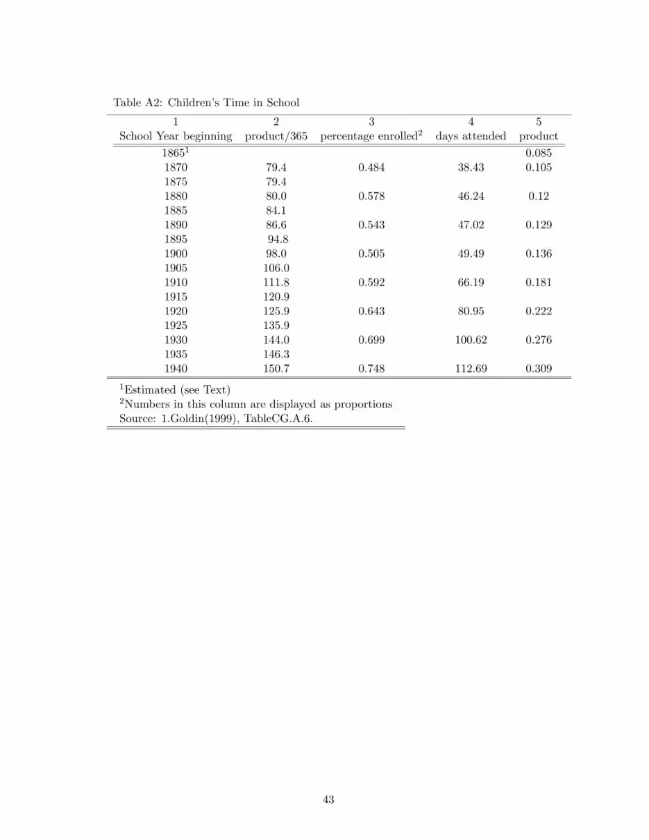
Table A2: Children’s Time in School

1 2 3 4 5School Year beginning product/365 percentage enrolled2 days attended product

18651 0.0851870 79.4 0.484 38.43 0.1051875 79.41880 80.0 0.578 46.24 0.121885 84.11890 86.6 0.543 47.02 0.1291895 94.81900 98.0 0.505 49.49 0.1361905 106.01910 111.8 0.592 66.19 0.1811915 120.91920 125.9 0.643 80.95 0.2221925 135.91930 144.0 0.699 100.62 0.2761935 146.31940 150.7 0.748 112.69 0.309

1Estimated (see Text)2Numbers in this column are displayed as proportionsSource: 1.Goldin(1999), TableCG.A.6.

43

.

References

[1] Adeshade, Marina (2009), “Female Labour Force Participation in an Era of Organizational and

Technological Change,”Canadian Journal of Economics, forthcoming.

[2] Albanesi, Stefania, and Claudia Olivetti (2007), “Gender Roles and Technological Progress”, CEPR

Discussion Paper No. DP6352 .

[3] Andreoni, James (1990), “Impure Altruism and Donations to Public Goods: A Theory of Warm-

Glow Giving”, Economic Journal, Vol. 100 (401), pp. 464-477.

[4] Bailey, Martha and William Collins (2011), “Did Improvements in Household Technology Cause

the Baby Boom? Evidence from Electrification, Appliance Diffusion, and the Amish” (with

William J. Collins), American Economic Journal-Macroeconomics, 3 (2), 189-217.

[5] Becker, Gary, (1981), A Treatise on the Family, Harvard University Press, Cambridge, Massa-

chusetts, and London England.

[6] – – – – – – and Robert J. Barro, (1988), “A Reformulation of the Economic Theory of Fertility”,

American Economic Review, Vol. CIII (1), pp:1-25.

[7] – – – – – – and Nigel Tomes, 1986, “Human Capital and the Rise and Fall of Families”, Journal

of Labor Economics, Vol. 4(3), pp:S1-S39.

[8] Browning Martin, Lars Peter Hansen and James J Heckman (1999), “Micro data and general

equilibrium models”, Handbook of Macroeconomics, in: J.B. Taylor and M. Woodford (ed),

Handbook of Macroeconomics, edition 1, Vol. 1, Chapter 8, pp: 543-633, Elsevier.

[9] Burnette, Joyce (2011), "The Emergence of Wage Discrimination in US Manufacturing", Wabash

College Working Paper.

[10] Card, David and Alan B. Krueger (1992), "Does School Quality Matter? Returns to Education

and the Characteristics of Public Schools in the United States", Journal of Political Economy,

100 (1): 1-40.

[11] Chiappori, Pierre-Andr´e.(1992) “Collective Labor Supply andWelfare.”Journal of Political Econ-

omy 100 (3): 437—467.

[12] Cvrcek, Tomas (2007), "Mothers, Wives and Workers: The Dynamics of White Fertility, Marriage

and Women’s Labor Supply in the United States 1870-1930", Vanderbilt Working Paper.

44

[13] De Vries, Jan (2008). The industrious revolution: consumer behavior and the household economy.

Cambridge University Press. Cambridge.

[14] Diamond, Jared (1997), Why is Sex Fun?, Basic Books, New York, NY.

[15] Doepke, Matthias (2005). "Child Mortality and Fertility Decline: Does the Barro-Becker Fit the

Facts?" Journal of Population Economics, 18(2), 337-366.

[16] ______________, and Fabrizio Zilibotti (2005)."The Macroeconomics of Child Labor Reg-

ulation," American Economic Review, 95(5), 1492-1524.

[17] – – – – – – – , and Michele Tertilt (2009). “Women’s Liberation: What’s in it for Men?”With

Michèle Tertilt, Quarterly Journal of Economics, 124(4), 1541-1591, November.

[18] – – – – – – – -(2011) "Does Female Empowerment Promote Economic Development?," North-

western University Working Paper.

[19] Fernández, Raquel, Alessandra Fogli and Claudia Olivetti (2004), “Mothers and Sons: Preference

Formation and Female Labor Force Dynamics”, Quarterly Journal of Economics, Vol. 119, No.

4, pp. 1,249-99.

[20] – – – and David Weil (1996), “The Gender Gap, Fertility, and Growth”, American Economic

Review, Vol. 89 (2), pp: 374-387.

[21] Wright Gavin (1986), Old South, New South: Revolutions in the Southern Economy Since the Civil

War, Basic Books, New York.

[22] Galor, Oded, and Joseph Ziera, (1993) “Income Distribution and Macroeconomics,”The Review

of Economic Studies, Vol. 60, No. 1., pp. 35-52.

[23] Goldin,Claudia (1990), Understanding the Gender Wage Gap, Oxford University Press, Oxford.

[24] _____________(1986), "The Earnings Gap Between Male and Female Workers: An His-

torical Perspective," NBER Working Paper, w1888.

[25] – – – – – – —(1999), "A Brief History of Education in the United States", NBER Working Paper

Series on Historical Factors in Long Run Growth Historical Paper 119.

[26] – – – – – and Lawrence Katz (2008), The Race between Education and Technology, Harvard

University Press, Cambridge, Massachusetts and London, England.

[27] – – – – – and Donald Parsons (1989), “Parental Altruism and Self-Interest: Child Labor among

Late-Nineteenth Century American Families”, Economic Inquiry, Vol. 27, pp: 637-659.

[28] – – – – – -Soloman Polachek (1987), "Residual Differences by Sex: Perspectives on the Gender

Gap in Earnings," American Economic Review, May (143-151)

45

[29] Greenwood, Jeremy, Ananth Seshadri and Mehmet Yorukoglu (2005) “Engines of Liberation”,

Review of Economic Studies, Vol. 72, pp. 109-33.

[30] Haines, Michael (2000), Economic History of the United States, Vol. II, Engerman Stanley J. and

Robert E. Gallman, ed., Cambridge University Press, Cambridge, UK

[31] Hazan, Moshe (2009), “Longevity and Lifetime Labor Supply: Evidence and Implications”, CEPR

DP 5963.

[32] – – – – – and Hosny Zoabi (2006), “Does longevity cause growth? A theoretical critique,”

Journal of Economic Growth, Vol. 11 (4), pp: 363- 376.

[33] Historical Statistics of the United States (2006), Millenial Edition, Volumes 1 and 2, Cambridge

University Press

[34] Jones, Larry and Michelle Tertilt (2007). "An Economic History of Fertility in the U.S.: 1826-1960"

forthcoming in book "Frontiers of Family Economics," Elsevier, edited by Peter Rupert.

[35] Lord, William (1989), "The Transition from Payroll to Consumption Receipts with Endogenous

Human Capital", Journal of Public Economics, Vol.38, pp: 53-73.

[36] – – – – – – (2002), Household Dynamics: Economic Growth and Policy, Oxford University Press,

Oxford.

[37] – – – and Peter Rangazas (1993), “Altruism, Deficit Policies, and the Wealth of Future Genera-

tions”, Economic Inquiry, Vol.XXXI, pp: 609-630.

[38] – – – – – – – – (2006), “Fertility and Development: The Roles of Schooling and Family Pro-

duction”, Journal of Economic Growth, Vol. 11, pp: 229-261.

[39] Margo, Robert A. (2000), Wages and Labor Markets in the United States, 1820-1860, University

of Chicago Press, Chicago and London.

[40] Miller, Grant (2008), "Women’s Suffrage, Political Responsiveness, and Child Survival in American

History", The Quarterly Journal of Economics, August 2008 pp: 1287-1326.

[41] Moehling, Carolyn (1999), "State Child Labor Laws and the Decline of Child Labor", Explorations

in Economic History, Vol.36, pp: 72-106.

[42] Mokyr, Joel (2000), “Why Was More Work for Mother? Knowledge and Household Behavior

1870-1945”, Journal of Economic History, Vol. 60 (1), pp: 1-41

[43] Murphy, Kevin, Curtis Simon and Robert Tamura (2008), “Fertility Decline, Baby Boom, and

Economic Growth”, Journal of Human Capital, Vol 2, No. 3, pp: 262-301.

46

[44] Olivetti, Claudia (2006). "Changes in women’s hours of market work: The role of returns to

experience," Review of Economic Dynamics, Vol. 9, pp: 557-587.

[45] Preston, Samuel H. and Michael R. Haines (1991), Fatal years: child mortality in late nineteenth-

century America, Princeton University Press, Princeton.

[46] Puerta Manuel J. (2009), “The Fewer, the Merrier - Compulsory Schooling Laws, Human Capital

and Fertility in the U.S.”, mimeo.

[47] Ramey, Valerie (2009), “Time Spent in Home Production in the Twentieth-Century United States:

New Estimates from Old Data”, The Journal of Economic History, Vol. 69, No. 1, pp: 1-47.

[48] Rangazas, Peter (2000), "Schooling and Economic Growth: A King-Rebelo Experiment with Hu-

man Capital," Journal of Monetary Economics, Vol. 46, pp: 397-416.

[49] – – – – – – (2002), "The Quantity and Quality of Schooling and U.S. Labor Productivity

Growth (1870-2000)", Review of Economic Dynamics, Vol. 5, pp: 932-964.

[50] Rendell, Michelle (2010), "Brain versus Brawn: The Realization of Women’s Comparative Advan-

tage, Mimeo.

[51] Roberts, Evan (2007), Her Real Sphere?: Married Women’s Labor Force Participation in the

United States 1860-1940. University of Minnesota Dissertation.

[52] Rotella, Elyce (1980), “Women’s Labor Force Participation and the Decline of the Family Economy

in the United States,”Explorations in Economic History, Vol. 17, pp: 95-117.

[53] – – – – – – (1981), From Home to Offi ce U.S. Women at Work 1870-1930, In R. Berkhofer, ed.,

Studies in American History and Culture, No. 25 Michigan, UMI Research Press.

[54] Soares, Rodrigo, and Bruno Falcao (2008), “The Demographic Transition and the Sexual Division

of Labor”, Journal of Political Economy, Vol. 116 (6), pp: 1058-1104.

[55] Sobek, Matthew (1997), A Century of Work: Gender, Labor Force Participation, and Occupational

Attainment in the United States, 1880-1990. University of Minnesota, Dissertation.

[56] United States Department of Agriculture (2006), “Costs of Children”,

http://www.cnpp.usda.gov/Publications/CRC/crc2006.pdf

[57] Wanamaker, Marianne (2010), "Did Industrialization Cause the American Fertility Decline? Evi-

dence from South Carolina", University of Tennessee Working Paper.

[58] Zelizer, Viviana A. (1985), Pricing the Priceless Child, Princeton University Press, Princeton.

47