Embed Size (px)
Citation preview
RHEOLOGICAL BEHAVIOR OF AN OBM SAMPLE OF THE GOM UNDER
XHPHT CONDITIONS
A Thesis
by
HUGO ANTONIO SANCHEZ TELESFORO
Submitted to the Office of Graduate and Professional Studies of
Texas A&M University
in partial fulfillment of the requirements for the degree of
MASTER OF SCIENCE
Chair of Committee, Jerome J. Schubert
Committee Members, Samuel Noynaert
Zenon Medina-Cetina
Head of Department, Daniel Hill
August 2017
Major Subject: Petroleum Engineering
Copyright 2017 Hugo Antonio Sanchez Telesforo
ii
ABSTRACT
The scope of this research is to study the rheological behavior of an oil based
mud (OBM) sample from the Mexican side of the Gulf of Mexico (GOM) under extreme
conditions of High Pressure High Temperature (HPHT). In the coming years many
HPHT wells are going to be drilled in this area of the GOM. Currently Mexican Oil and
Gas industry is already open to international operators because the Mexican energy
reform has been approved, so it is important to study the possible drilling fluids that will
be used. These fluids can be within any of these 3 tiers of HPHT classification: HPHT,
ultra (uHPHT) or extreme (xHPHT).
The sample was submitted to extreme HPHT conditions, by using the state-of-
the-art Model 7600 HPHT Viscometer that is capable of measuring drilling fluid
properties up to 40,000 psi and 600 °F. During the laboratory tests performance, it was
noticed that erroneous results were obtained by several mechanical failures. It should be
noted that the spare parts take a long time to arrive-around 3 weeks. One of the failures
was that the pivot of the spring assembly got inside the device, so the bob was spinning
nonstop. For this reason the readings of the dial went well beyond the allowed range;
another mechanical failure was that the spring of the spring assembly was loose, which
did not allow us to obtain a correct reading of shear stress at high pressures and low
temperatures; also the baffle does not separate the pressurizing oil from the sample,
mixing these two fluids and obviously affecting the properties of the sample. This was

iii
noticed by running one test with baffle and another without it getting very similar
results.
The rheological behavior of the sample showed that the viscosity is inversely
proportional to temperature and directly proportional to pressure, noticing a failure point
at 300 °F, because of sample degradation.
Moreover the rheogram´s curves obtained are quite similar to a second degree
polynomial function, with R-squared values ranging from 0.95 to 0.99; hence an
equation can be adjusted in the future by extrapolating different pressure and
temperature values.

iv
DEDICATION
This work is dedicated to my beautiful wife and two daughters.

v
ACKNOWLEDGEMENTS
I would like to thank my committee chair, Dr. Schubert, and my committee
members, Dr. Noynaert and Dr. Medina-Cetina, for their guidance and support
throughout the course of this research.
Thanks also to my friends and colleagues and the department faculty and staff for
making my time at Texas A&M University a great experience, especially to Erick Rafael
Martinez Antunez and Pedro Cavalcanti de Sousa.
Thanks to my wife and my two daughters for their patience and love.
Finally, thanks to my mother, father and brother for their encouragement.
vi
CONTRIBUTORS AND FUNDING SOURCES
Contributors
This work was supervised by a thesis committee consisting of Professor Dr.
Schubert [advisor] and Dr. Noynaert of the Department of Petroleum Engineering and
Professor Dr. Medina-Cetina of the Department of Civil Engineering.
All work for the thesis was completed independently by the student.
Funding Sources
Graduate study was supported by a fellowship from CONACYT-SENER
Hidrocarburos.
This work was made possible in part by Pemex E&P.
vii
NOMENCLATURE
API American Petroleum Institute
BHDF Baker Hughes Drilling Fluids
BHP Bottom Hole Pressure
BHT Bottom Hole Temperature
CaCl Calcium Chloride
CaCO3 Calcium Carbonate
CMC Carboxymethyl cellulose
cP Centipoise
DEA Danish Energy Agency
EBF Emulsion Based Drilling Fluid
ECD Equivalent Circulating Density
Shear Rate
GOM Gulf of Mexico
H2S Hydrogen Sulfide
HPHT High Pressure High Temperature
HPWBM High Performance Water Based Mud
HSE Health, Safety and Environment
ISO International Organization for Standardization
KCl Potassium Chloride
LSRV Low Shear Rate Viscosity
viii
LWD Logging While Drilling
p Plastic Viscosity
Mn3O4 Manganese Tetroxide
MPa Mega Pascal
MPD Managed Pressure Drilling
MSDS Material Safety Data Sheet
MW Mud Weight
MWCNT Multiwall Carbon Nanotubes
MWD Measurement While Drilling
NaCl Sodium Chloride
NADF Non-Aqueous Drilling Fluids
NETL National Energy Technology Laboratory
nm Nautical Miles
OBM Oil Based Mud
OCS Outer Continental Shelf
OWR Oil Water Ratio
PA Polyamide
PDC Polycrystalline Diamond Compact
PHPA Partially Hydrolyzed Polyacrylamide
ppb Parts Per Billion
PPE Personal Protective Equipment
ppg Pounds Per Gallon
ix
PV Plastic Viscosity
PWD Pressure While Drilling
ROP Rate of Penetration
RPM Revolutions Per Minute
SBM Synthetic Based Mud
Shear Stress
TSP Thermally Stable Polycrystalline
TVD True Vertical Depth
y Yield Point
uHPHT Ultra High Pressure High Temperature
VES Viscoelastic Surfactant
WBM Water Based Mud
xHPHT Extreme High Pressure High Temperature
YP Yield Point
x
TABLE OF CONTENTS
Page
ABSTRACT ..................................................................................................................... ii
DEDICATION ................................................................................................................. iv
ACKNOWLEDGEMENTS .............................................................................................. v
CONTRIBUTORS AND FUNDING SOURCES ........................................................... vi
NOMENCLATURE ....................................................................................................... vii
TABLE OF CONTENTS ................................................................................................. x
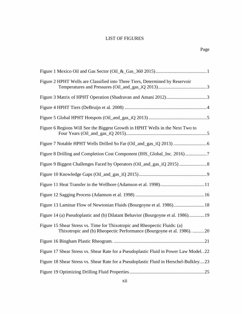
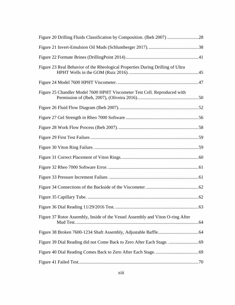
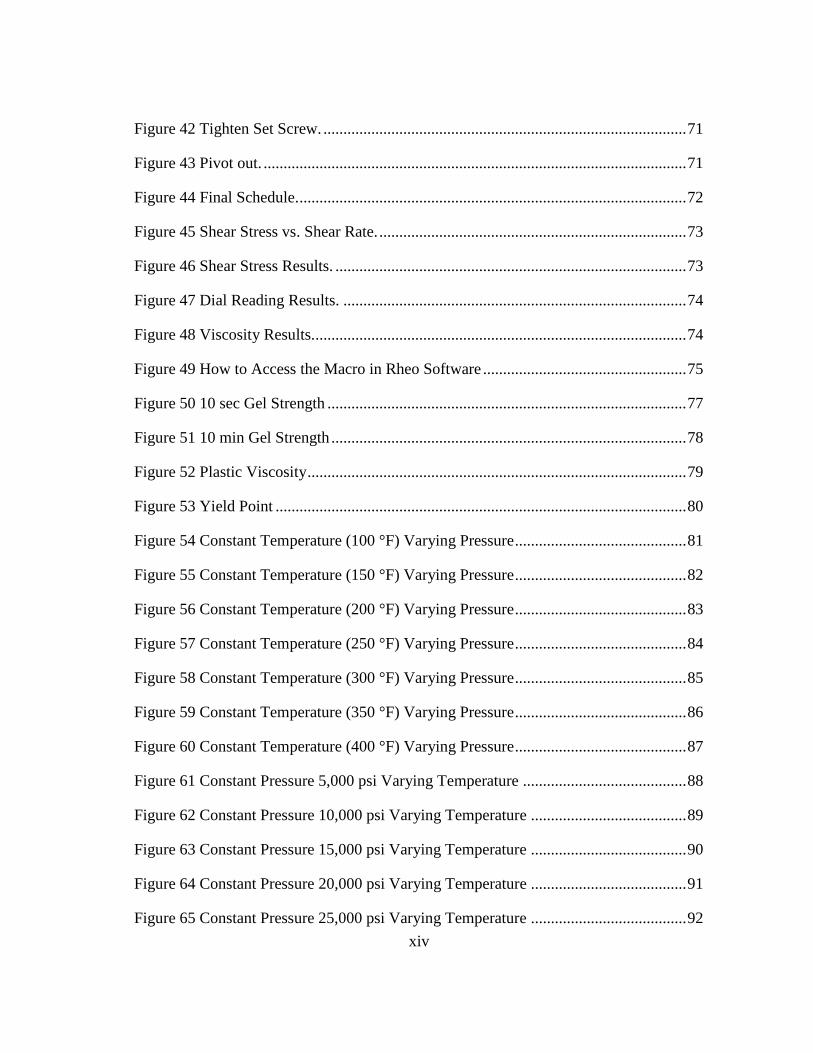
LIST OF FIGURES ........................................................................................................ xii
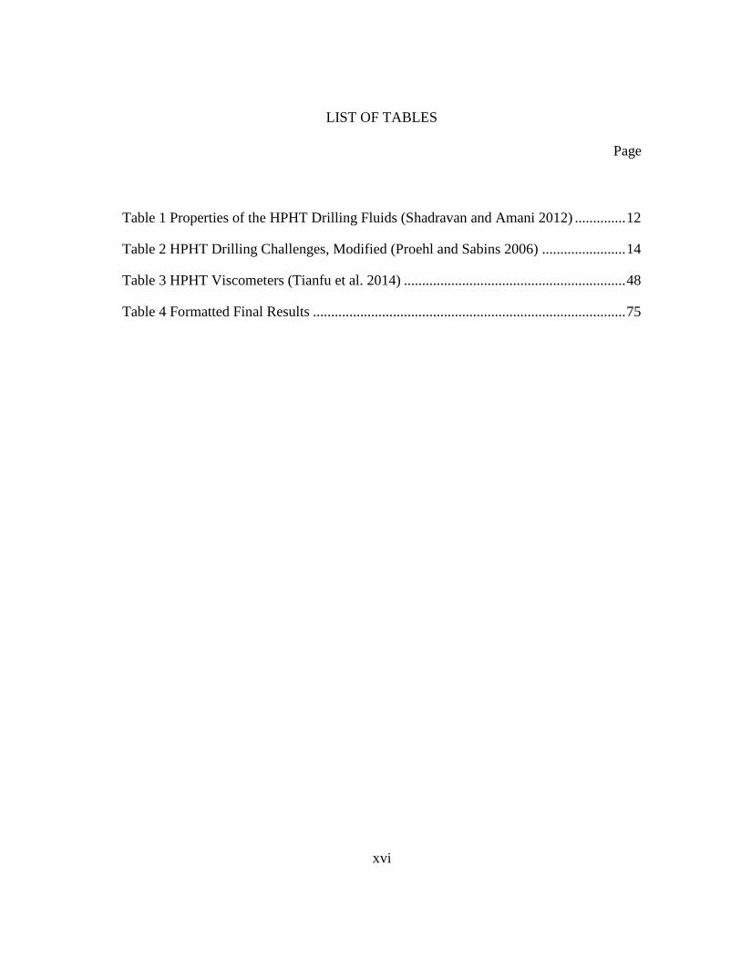
LIST OF TABLES ......................................................................................................... xvi
CHAPTER I INTRODUCTION ....................................................................................... 1
CHAPTER II LITERATURE REVIEW .......................................................................... 2
2.1 HPHT Wells ........................................................................................................ 2
2.1.1 Classification ............................................................................................... 2
2.1.2 Location ....................................................................................................... 4
2.1.3 Costs ............................................................................................................ 6
2.2 HPHT Challenges ............................................................................................... 7
2.2.1 Gaps ............................................................................................................. 7
2.2.2 Sagging ...................................................................................................... 15
2.3 Rheological Models .......................................................................................... 18
2.3.1 Overview of Rheological Models .............................................................. 18
2.3.2 Bingham Plastic ......................................................................................... 21
2.3.3 Power Law ................................................................................................. 22
2.3.4 Herschel-Bulkley ....................................................................................... 23
2.3.5 Rheometers and Viscometers .................................................................... 24
2.4 HPHT Drilling Fluids ........................................................................................ 25
2.4.1 Functions of Drilling Fluids ....................................................................... 26
2.4.2 Drilling-Fluid Categories and Classification ............................................. 27
2.4.2.1 WBMs ................................................................................................ 28
2.4.2.2 OBMs ................................................................................................. 31
xi
2.4.2.3 Formate Brines ........................................................................................ 40
2.4.3 Drilling Fluids of Ultra HPHT Well on the GOM Mexican Side …............... 44
CHAPTER III EQUIPMENT AND METHODOLOGY ..................................................... 47
3.1 Model 7600 HPHT Viscometer .............................................................................. 47
3.2 Experimental Setup ................................................................................................. 49
3.3 Experimental Procedure .......................................................................................... 52
3.3.1 Fluid Type ....................................................................................................... 53
3.3.2 Sample ............................................................................................................. 53
3.3.3 Fluid Preparation ............................................................................................. 53
3.4 Experimental Schedule ........................................................................................... 54
3.5 Equipment Problems ............................................................................................... 58
3.6 Future Improvements .............................................................................................. 65
3.7 Safety ...................................................................................................................... 66
CHAPTER IV RESULTS OF EXPERIMENTS AND DISCUSSION ................................ 69
4.1 Constant Temperature Varying Pressure ................................................................ 80
4.2 Constant Pressure Varying Temperature ................................................................ 87
CHAPTER V CONCLUSIONS, RECOMMENDATIONS AND FUTURE WORK …..... 96
REFERENCES ..................................................................................................................... 98
xii
LIST OF FIGURES
Page
Figure 1 Mexico Oil and Gas Sector (Oil_&_Gas_360 2015) ........................................... 1
Figure 2 HPHT Wells are Classified into Three Tiers, Determined by Reservoir
Temperatures and Pressures (Oil_and_gas_iQ 2013) ......................................... 3
Figure 3 Matrix of HPHT Operation (Shadravan and Amani 2012) .................................. 3
Figure 4 HPHT Tiers (DeBruijn et al. 2008) ..................................................................... 4
Figure 5 Global HPHT Hotspots (Oil_and_gas_iQ 2013) ................................................. 5
Figure 6 Regions Will See the Biggest Growth in HPHT Wells in the Next Two to
Four Years (Oil_and_gas_iQ 2015) .................................................................... 5
Figure 7 Notable HPHT Wells Drilled So Far (Oil_and_gas_iQ 2013) ............................ 6
Figure 8 Drilling and Completion Cost Component (IHS_Global_Inc. 2016) .................. 7
Figure 9 Biggest Challenges Faced by Operators (Oil_and_gas_iQ 2015) ....................... 8
Figure 10 Knowledge Gaps (Oil_and_gas_iQ 2015) ......................................................... 9
Figure 11 Heat Transfer in the Wellbore (Adamson et al. 1998) ..................................... 11
Figure 12 Sagging Process (Adamson et al. 1998) .......................................................... 16
Figure 13 Laminar Flow of Newtonian Fluids (Bourgoyne et al. 1986) .......................... 18
Figure 14 (a) Pseudoplastic and (b) Dilatant Behavior (Bourgoyne et al. 1986). ............ 19
Figure 15 Shear Stress vs. Time for Thixotropic and Rheopectic Fluids: (a)
Thixotropic and (b) Rheopectic Performance (Bourgoyne et al. 1986). .......... 20
Figure 16 Bingham Plastic Rheogram. ............................................................................ 21
Figure 17 Shear Stress vs. Shear Rate for a Pseudoplastic Fluid in Power Law Model. . 22
Figure 18 Shear Stress vs. Shear Rate for a Pseudoplastic Fluid in Herschel-Bulkley. ... 23
Figure 19 Optimizing Drilling Fluid Properties ............................................................... 25
xiii
Figure 20 Drilling Fluids Classification by Composition. (Ibeh 2007) ........................... 28
Figure 21 Invert-Emulsion Oil Muds (Schlumberger 2017). ........................................... 38
Figure 22 Formate Brines (DrillingPoint 2014) ............................................................... 41
Figure 23 Real Behavior of the Rheological Properties During Drilling of Ultra
HPHT Wells in the GOM (Ruiz 2016). ............................................................ 45
Figure 24 Model 7600 HPHT Viscometer. ...................................................................... 47
Figure 25 Chandler Model 7600 HPHT Viscometer Test Cell. Reproduced with
Permission of (Ibeh, 2007), (Oliveira 2016). .................................................... 50
Figure 26 Fluid Flow Diagram (Ibeh 2007). .................................................................... 52
Figure 27 Gel Strength in Rheo 7000 Software ............................................................... 56
Figure 28 Work Flow Process (Ibeh 2007). ..................................................................... 58
Figure 29 First Test Failure. ............................................................................................. 59
Figure 30 Viton Ring Failure. .......................................................................................... 59
Figure 31 Correct Placement of Viton Rings. .................................................................. 60
Figure 32 Rheo 7000 Software Error. .............................................................................. 61
Figure 33 Pressure Increment Failure. ............................................................................. 61
Figure 34 Connections of the Backside of the Viscometer. ............................................. 62
Figure 35 Capillary Tube. ................................................................................................ 62
Figure 36 Dial Reading 11/29/2016 Test. ........................................................................ 63
Figure 37 Rotor Assembly, Inside of the Vessel Assembly and Viton O-ring After
Mud Test. .......................................................................................................... 64
Figure 38 Broken 7600-1234 Shaft Assembly, Adjustable Baffle. .................................. 64
Figure 39 Dial Reading did not Come Back to Zero After Each Stage. .......................... 69
Figure 40 Dial Reading Comes Back to Zero After Each Stage. ..................................... 69
Figure 41 Failed Test. ....................................................................................................... 70
xiv
Figure 42 Tighten Set Screw. ........................................................................................... 71
Figure 43 Pivot out. .......................................................................................................... 71
Figure 44 Final Schedule. ................................................................................................. 72
Figure 45 Shear Stress vs. Shear Rate. ............................................................................. 73
Figure 46 Shear Stress Results. ........................................................................................ 73
Figure 47 Dial Reading Results. ...................................................................................... 74
Figure 48 Viscosity Results. ............................................................................................. 74
Figure 49 How to Access the Macro in Rheo Software ................................................... 75
Figure 50 10 sec Gel Strength .......................................................................................... 77
Figure 51 10 min Gel Strength ......................................................................................... 78
Figure 52 Plastic Viscosity ............................................................................................... 79
Figure 53 Yield Point ....................................................................................................... 80
Figure 54 Constant Temperature (100 °F) Varying Pressure ........................................... 81
Figure 55 Constant Temperature (150 °F) Varying Pressure ........................................... 82
Figure 56 Constant Temperature (200 °F) Varying Pressure ........................................... 83
Figure 57 Constant Temperature (250 °F) Varying Pressure ........................................... 84
Figure 58 Constant Temperature (300 °F) Varying Pressure ........................................... 85
Figure 59 Constant Temperature (350 °F) Varying Pressure ........................................... 86
Figure 60 Constant Temperature (400 °F) Varying Pressure ........................................... 87
Figure 61 Constant Pressure 5,000 psi Varying Temperature ......................................... 88
Figure 62 Constant Pressure 10,000 psi Varying Temperature ....................................... 89
Figure 63 Constant Pressure 15,000 psi Varying Temperature ....................................... 90
Figure 64 Constant Pressure 20,000 psi Varying Temperature ....................................... 91
Figure 65 Constant Pressure 25,000 psi Varying Temperature ....................................... 92

xv
Figure 66 Constant Pressure 30,000 psi Varying Temperature ....................................... 93
Figure 67 Constant Pressure 35,000 psi Varying Temperature ....................................... 94
xvi
LIST OF TABLES
Page
Table 1 Properties of the HPHT Drilling Fluids (Shadravan and Amani 2012) .............. 12
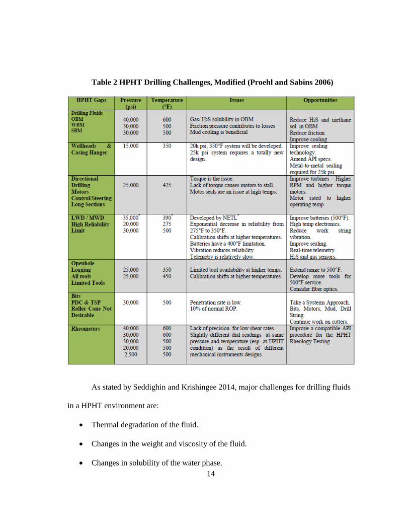
Table 2 HPHT Drilling Challenges, Modified (Proehl and Sabins 2006) ....................... 14
Table 3 HPHT Viscometers (Tianfu et al. 2014) ............................................................. 48
Table 4 Formatted Final Results ...................................................................................... 75
1
CHAPTER I
INTRODUCTION
The term HPHT was first coined in the 1990 Cullen Report published in the
aftermath of the Piper Alpha platform disaster. Generally used to describe wells of a
hotter or higher pressure than most, HPHT wells have become increasingly
commonplace in a world of dwindling conventional reserves.
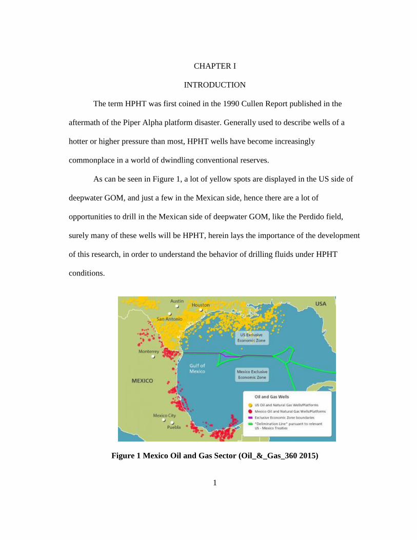
As can be seen in Figure 1, a lot of yellow spots are displayed in the US side of
deepwater GOM, and just a few in the Mexican side, hence there are a lot of
opportunities to drill in the Mexican side of deepwater GOM, like the Perdido field,
surely many of these wells will be HPHT, herein lays the importance of the development
of this research, in order to understand the behavior of drilling fluids under HPHT
conditions.
Figure 1 Mexico Oil and Gas Sector (Oil_&_Gas_360 2015)
2
CHAPTER II
LITERATURE REVIEW
2.1 HPHT Wells
In HPHT environments there are frequently narrow operational windows
between pore and fracture pressure which requires drilling fluids designed to minimize
Equivalent Circulating Density (ECD), (De Stefano, Stamatakis, and Young 2012).
2.1.1 Classification
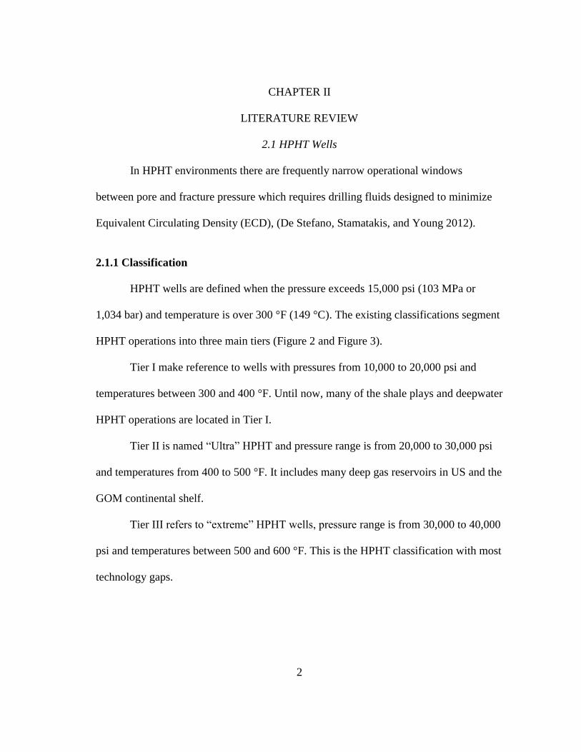
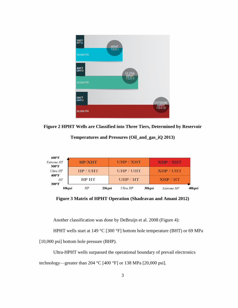
HPHT wells are defined when the pressure exceeds 15,000 psi (103 MPa or
1,034 bar) and temperature is over 300 °F (149 °C). The existing classifications segment
HPHT operations into three main tiers (Figure 2 and Figure 3).
Tier I make reference to wells with pressures from 10,000 to 20,000 psi and
temperatures between 300 and 400 °F. Until now, many of the shale plays and deepwater
HPHT operations are located in Tier I.
Tier II is named ―Ultra‖ HPHT and pressure range is from 20,000 to 30,000 psi
and temperatures from 400 to 500 °F. It includes many deep gas reservoirs in US and the
GOM continental shelf.
Tier III refers to ―extreme‖ HPHT wells, pressure range is from 30,000 to 40,000
psi and temperatures between 500 and 600 °F. This is the HPHT classification with most
technology gaps.
3
Figure 2 HPHT Wells are Classified into Three Tiers, Determined by Reservoir
Temperatures and Pressures (Oil_and_gas_iQ 2013)
Figure 3 Matrix of HPHT Operation (Shadravan and Amani 2012)
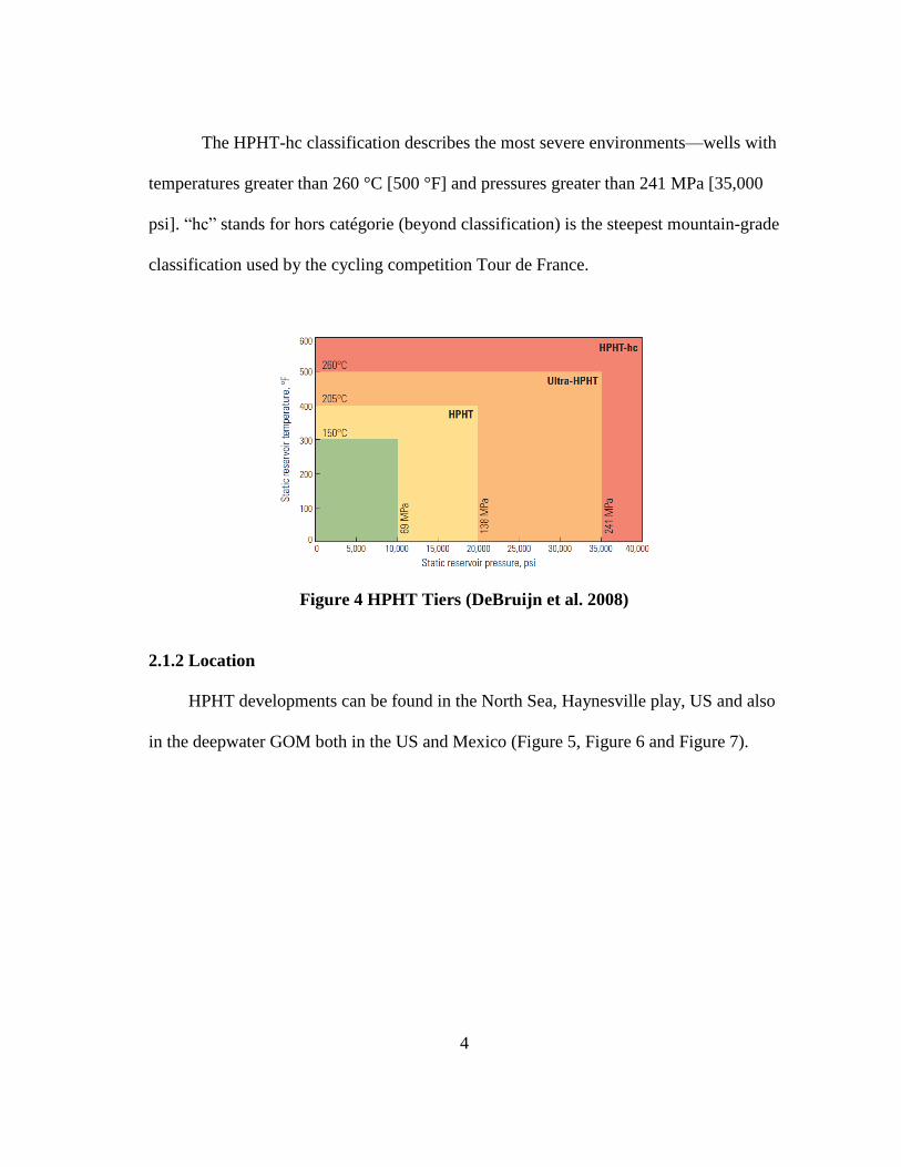
Another classification was done by DeBruijn et al. 2008 (Figure 4):
HPHT wells start at 149 °C [300 °F] bottom hole temperature (BHT) or 69 MPa
[10,000 psi] bottom hole pressure (BHP).
Ultra-HPHT wells surpassed the operational boundary of prevail electronics
technology—greater than 204 °C [400 °F] or 138 MPa [20,000 psi].
4
The HPHT-hc classification describes the most severe environments—wells with
temperatures greater than 260 °C [500 °F] and pressures greater than 241 MPa [35,000
psi]. ―hc‖ stands for hors catégorie (beyond classification) is the steepest mountain-grade
classification used by the cycling competition Tour de France.
Figure 4 HPHT Tiers (DeBruijn et al. 2008)
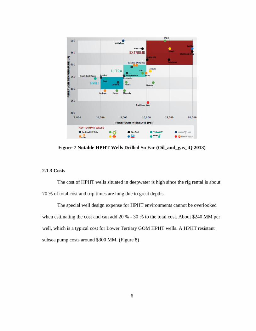
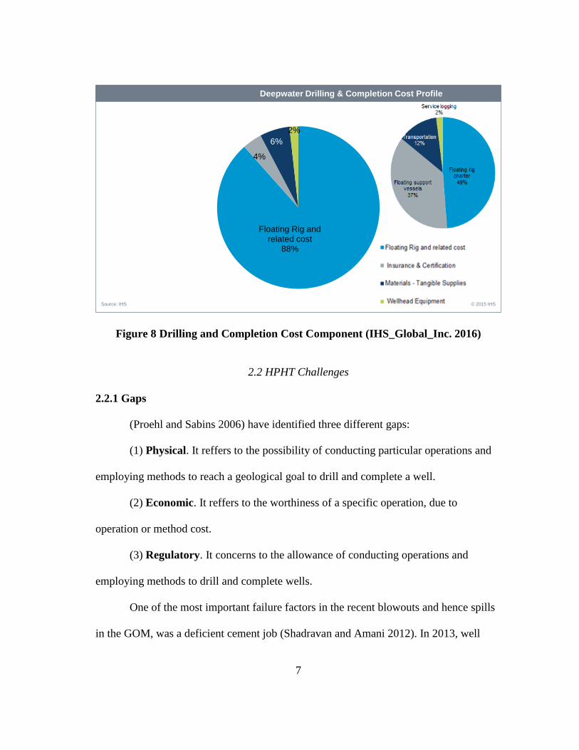
2.1.2 Location
HPHT developments can be found in the North Sea, Haynesville play, US and also
in the deepwater GOM both in the US and Mexico (Figure 5, Figure 6 and Figure 7).
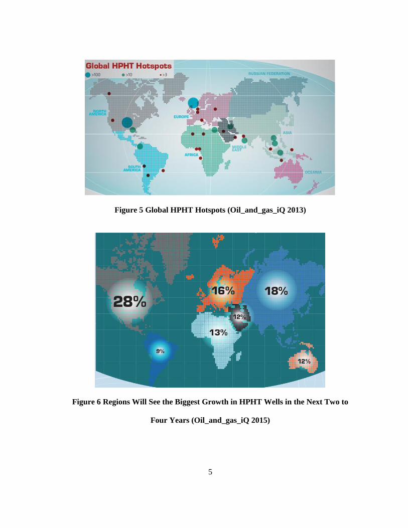
5
Figure 5 Global HPHT Hotspots (Oil_and_gas_iQ 2013)
Figure 6 Regions Will See the Biggest Growth in HPHT Wells in the Next Two to
Four Years (Oil_and_gas_iQ 2015)
6
Figure 7 Notable HPHT Wells Drilled So Far (Oil_and_gas_iQ 2013)
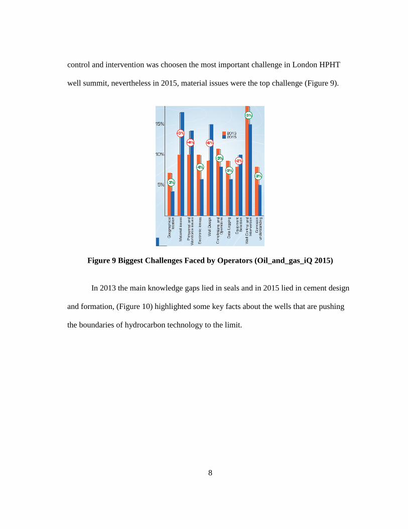
2.1.3 Costs
The cost of HPHT wells situated in deepwater is high since the rig rental is about
70 % of total cost and trip times are long due to great depths.
The special well design expense for HPHT environments cannot be overlooked
when estimating the cost and can add 20 % - 30 % to the total cost. About $240 MM per
well, which is a typical cost for Lower Tertiary GOM HPHT wells. A HPHT resistant
subsea pump costs around $300 MM. (Figure 8)
7
Figure 8 Drilling and Completion Cost Component (IHS_Global_Inc. 2016)
2.2 HPHT Challenges
2.2.1 Gaps
(Proehl and Sabins 2006) have identified three different gaps:
(1) Physical. It reffers to the possibility of conducting particular operations and
employing methods to reach a geological goal to drill and complete a well.
(2) Economic. It reffers to the worthiness of a specific operation, due to
operation or method cost.
(3) Regulatory. It concerns to the allowance of conducting operations and
employing methods to drill and complete wells.
One of the most important failure factors in the recent blowouts and hence spills
in the GOM, was a deficient cement job (Shadravan and Amani 2012). In 2013, well
Floating Rig and related cost
88%
4%
6%
2%
Cost Deepwater Drilling & Completion Cost Profile
Source: IHS © 2015 IHS
8
control and intervention was choosen the most important challenge in London HPHT
well summit, nevertheless in 2015, material issues were the top challenge (Figure 9).
Figure 9 Biggest Challenges Faced by Operators (Oil_and_gas_iQ 2015)
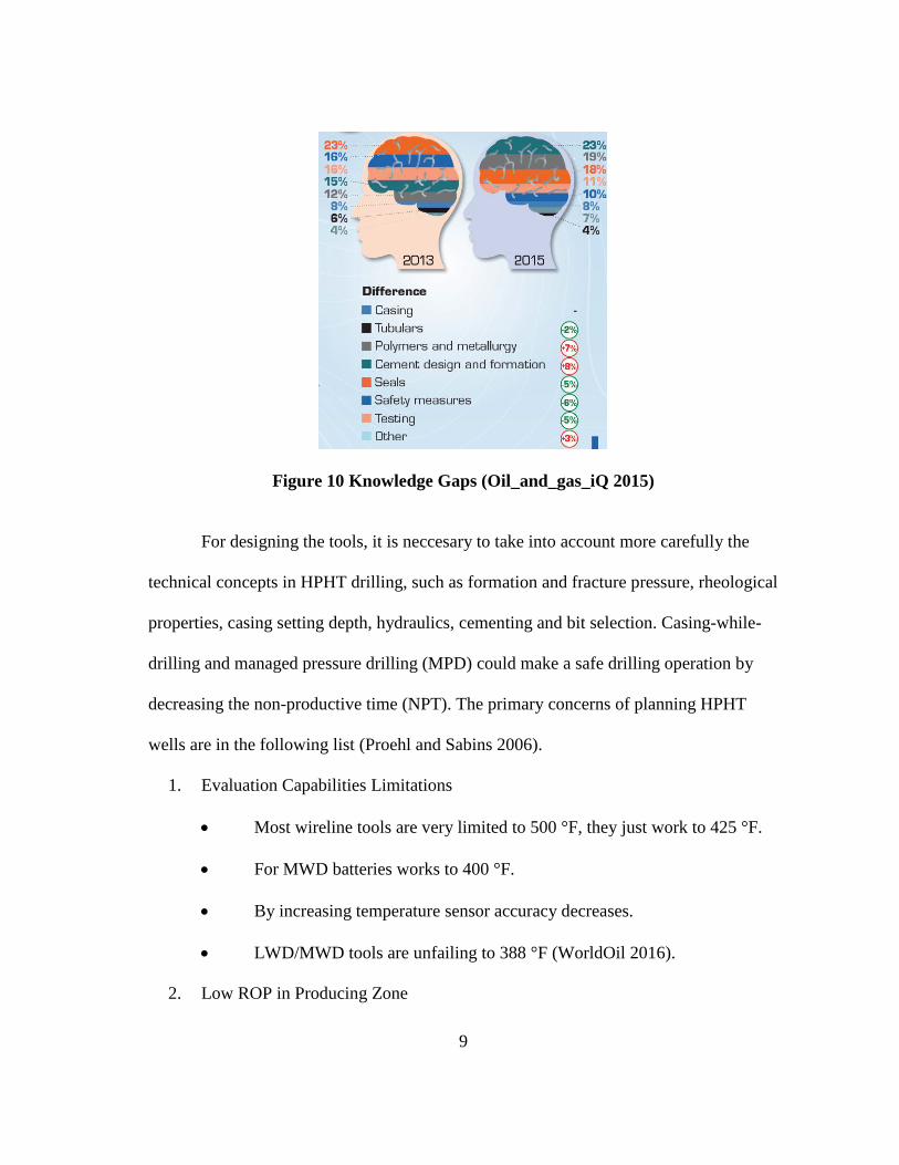
In 2013 the main knowledge gaps lied in seals and in 2015 lied in cement design
and formation, (Figure 10) highlighted some key facts about the wells that are pushing
the boundaries of hydrocarbon technology to the limit.
9
Figure 10 Knowledge Gaps (Oil_and_gas_iQ 2015)
For designing the tools, it is neccesary to take into account more carefully the
technical concepts in HPHT drilling, such as formation and fracture pressure, rheological
properties, casing setting depth, hydraulics, cementing and bit selection. Casing-while-
drilling and managed pressure drilling (MPD) could make a safe drilling operation by
decreasing the non-productive time (NPT). The primary concerns of planning HPHT
wells are in the following list (Proehl and Sabins 2006).
1. Evaluation Capabilities Limitations
Most wireline tools are very limited to 500 °F, they just work to 425 °F.
For MWD batteries works to 400 °F.
By increasing temperature sensor accuracy decreases.
LWD/MWD tools are unfailing to 388 °F (WorldOil 2016).
2. Low ROP in Producing Zone

10
Compared to normal drilling for GOM wells bits commonly remove 10 %
of the rock (Radwan and Karimi 2011).
In PDC bits crystalline structure breaks down.
Impregnated cutter drilling is slow.
Roller-cone bits are inappropiate.
ROP has been improved by a better turbines and motor designs.
To improve reliability and penetration rates; motor, bit, mud and drill
string dynamics must be optimized as a whole.
Eventhough high torque solutions are offered by pumps, torque is a issue.
3. Well Control
Owing to lithology and geopressure, fluid loss is an issue.
The drilling window is very narrow.
Solubility of H2S (hydrogen sulfide) and methane in OBM.
Mud storage because of Hole Ballooning.
It is needed a well head design for 25,000 psi and 450 °F, according to
Pallanich 2015, current design is 20,000 psi and 350 °F.
4. Non-Productive Time
Tool failure and bit trips.
Stuck pipe and twisting off.
Decision making due to lack of experience.
11
More hydraulic stability in HPHT/MPD or underbalanced drilling (UBD)
operations is provided by continuous circulation drilling. Conventional circulation
damaging drilling components or causing well control.
Safety issues due to handling HT materials.
5. Drilling Fluid
Reduce friction pressure and improve ECD.
Coolant for LWD/MWD tools.
Barite Sag.
Drilling Fluid Loss.
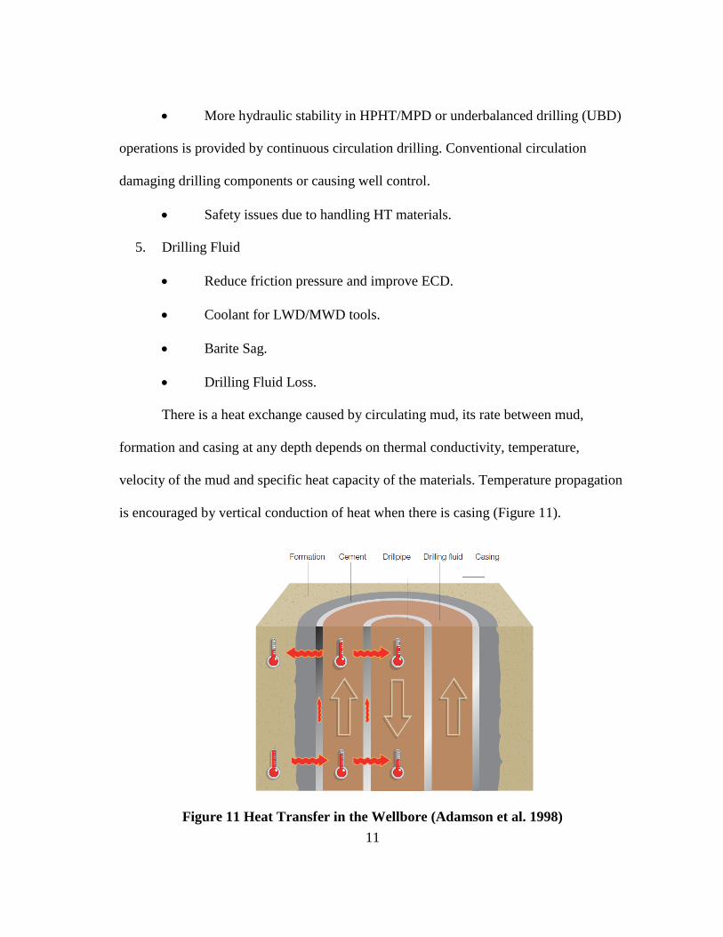
There is a heat exchange caused by circulating mud, its rate between mud,
formation and casing at any depth depends on thermal conductivity, temperature,
velocity of the mud and specific heat capacity of the materials. Temperature propagation
is encouraged by vertical conduction of heat when there is casing (Figure 11).
Figure 11 Heat Transfer in the Wellbore (Adamson et al. 1998)
12
Shadravan, Amani, Beck, Schubert, Zigmond and Ravi have done many HPHT
tests on OBM and Water Based Muds (WBM) of US and Qatar fields using the Model
7600 HPHT Viscometer. Lee, Shadravan and Young analyzed the behavior of many
HPHT Rheometers, by the study of rheological properties of a HPHT OBM they made
suggestions to the American Petroleum Institute (API) committee (Amani 2012, Amani
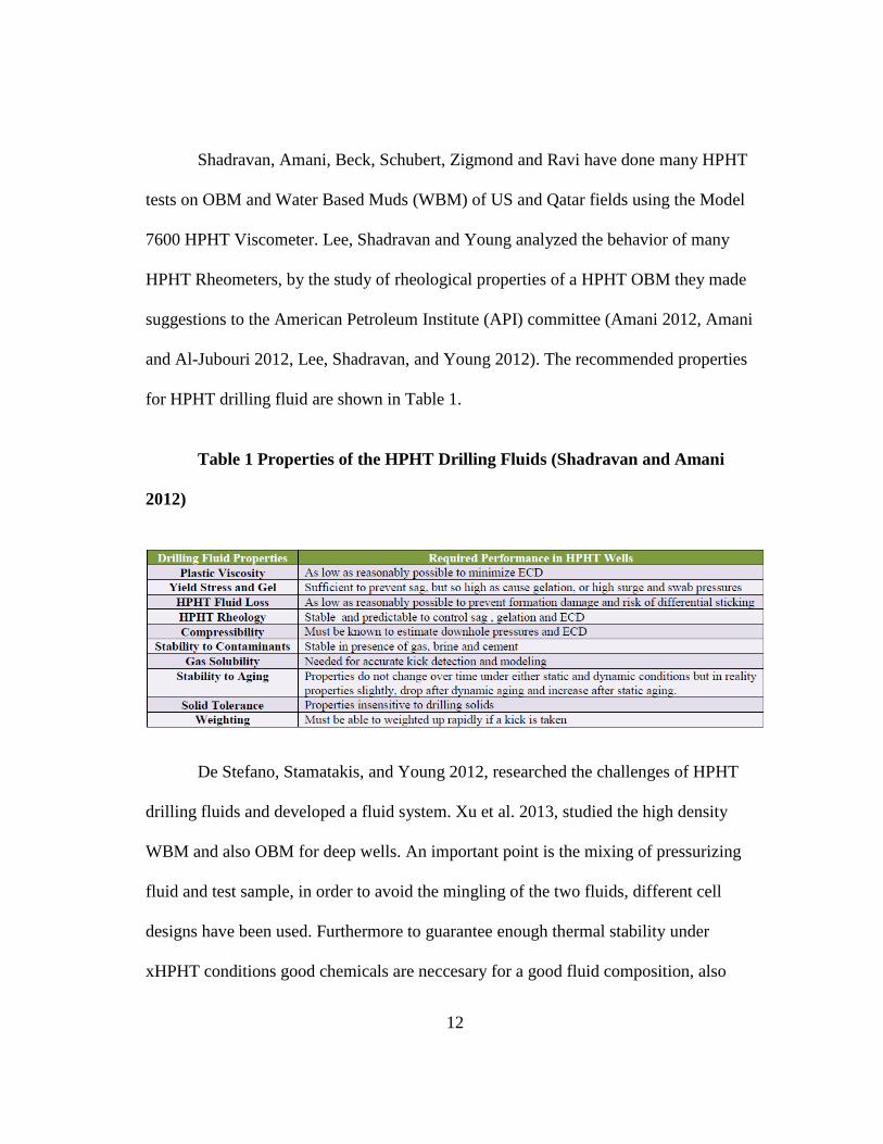
and Al-Jubouri 2012, Lee, Shadravan, and Young 2012). The recommended properties
for HPHT drilling fluid are shown in Table 1.
Table 1 Properties of the HPHT Drilling Fluids (Shadravan and Amani
2012)
De Stefano, Stamatakis, and Young 2012, researched the challenges of HPHT
drilling fluids and developed a fluid system. Xu et al. 2013, studied the high density
WBM and also OBM for deep wells. An important point is the mixing of pressurizing
fluid and test sample, in order to avoid the mingling of the two fluids, different cell
designs have been used. Furthermore to guarantee enough thermal stability under
xHPHT conditions good chemicals are neccesary for a good fluid composition, also
13
more research is needed to develop this products. Without a good thermal stability,
simulation using data gotten at low pressure and temperature is unreliable, (Lee,
Shadravan, and Young 2012).
The design of the hydraulics of the fluid depend on the affectance level of the
fluid rheology by pressure and temperature in the wellbore. If these effects are ignored
there are going to be errors with repair costs required during later stages of drilling. The
main goal of the design of a drilling fluid is to mantain its properties in the wellbore. The
rheological properties determine the capability of the fluid to carry cuttings and the
amount of the drop of the friction pressure that happens during its circulation. This
friction pressure drop, determine the pump pressure to keep circulation and the
increment in pressure during circulation at the base of the wellbore (ECD).
It is neccesary to predict and control ECD for avoiding the fracture of the
formation and lost circulation during drilling operations with narrow operating windows,
it might generate well control and wellbore stability problems. The degree of the
influence of temperature and pressure in fluid rheology is more difficult to predict than
in density. The ECD and the hole cleaning capacity are affected by rheological
properties changes. In deviated holes this problem is bigger, hole cleaning problems can
cause a sidetrack that is time consuming and hence expensive, or in the worst scenario a
well abandonment. The rheological changes in the wellbore have to be taken into
account. Zamora studied the performance under xHPHT conditions of oils, synthetics
and brines used to made OBM, Synthetic Based Muds (SBM), and WBM respectively
(Zamora et al. 2012) Table 2.
14
Table 2 HPHT Drilling Challenges, Modified (Proehl and Sabins 2006)
As stated by Seddighin and Krishingee 2014, major challenges for drilling fluids
in a HPHT environment are:
Thermal degradation of the fluid.
Changes in the weight and viscosity of the fluid.
Changes in solubility of the water phase.
15
Expansion and compression of the fluid, especially when using invert emulsions.
According to Marinescu, Young, and Iskander 2014, the list of challenges is still
extended by operational issues:
ECD – vital if the drilling mud weight (MW) window is narrow or the well
construction dictate slim holes into the reservoir;
High-Temperature Gelation – caused by the flocculation of clay or solids in mud.
This requires a very tight control of the solids content and selecting thermal stable
products for treatment;
HPHT Fluid Loss – is affected by HT gelation and degradation and increases
with temperature; for tight reservoirs it is very important to keep it very low, since
mainly the filtrate invasion is the principal formation damage;
Product Degradation – Can change all mud properties and system stability, it is
time and temperature dependent;
High solids content – elevates PV and compounds gelation related problems;
Barite sag – a dynamic and static mechanism when high densities are necessary.
2.2.2 Sagging
It occurs when mud solids fall, caused by segregation. The principal problem
generated is the difficulty of controlling BHPs. Heavy mud can produce induced
fractures and lost circulation, in the other hand light mud allows formation fluid influx
and wellbore instability. Both dynamic and static conditions sagging can be presented;
the best condition is under low shear rate conditions prior to achieve static viscosity.
16
High-quality barite is vital for HPHT mud due to poor particle size distribution or
impurities can generate big troubles intensified by HPHT conditions (Adamson et al.
1998).
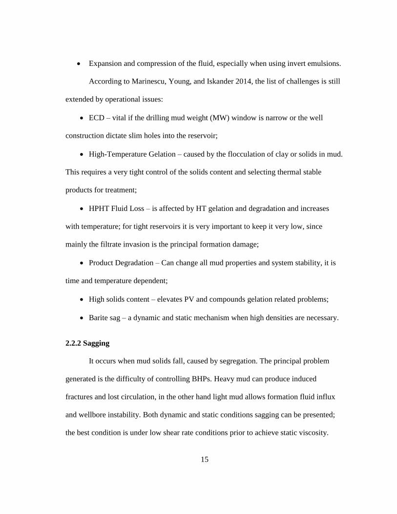
Gravity may cause weighting material when there is not enough circulation (a). A
barite accumulation at the bottom of the hole is caused by sagging (b). The barite
accumulations can collapse the bottom of the wellbores (c). Finally, collapse can cause
barite accumulation and thus the density can vary significantly (d) (Figure 12)
According to Adamson et al. 1998, during sagging, the viscosity is lowered by shear
thinning because of the motion of the solids.
Figure 12 Sagging Process (Adamson et al. 1998)
De Stefano, Stamatakis, and Young 2013, studied how to help maintain
suspension and minimize the settling and sag issues, by selecting a weighting material
which was comprised of a high grade barite that was milled to an average particle size
less than 2 microns. Typically the smaller the particulate size, the easier to suspend the
particles in a fluid. In this particular case where micronized barite (D50<2 micron) is
17
much smaller than the API-grade barite (D50<45 micron), the measured static and
dynamic sag of the weight material was very low.
The benefit of the micronized barite on drilling fluids and drilling operations can
be listed as:
For the same ECD, reduced pump pressure
Improved ECD management in narrow hydraulic operating margins
Reduced risk of ECD-related losses
Reduced swab, surge and circulating pressure
Improved Pressure While Drilling (PWD), MWD and LWD signal responses
The need of fluids for temperatures over 300 °F has grown more than the
capacity of conventional bio-polymers to create rheological stable fluids. The HPHT
drilling fluids, tend to sag; they also have syneresis where gel structure expels liquid;
this calls for the need of a HPHT drilling fluid with anti-sagging abilities and high low
shear rate viscosity (LSRV), to deal with this, Shah, Shanker, and Ogugbue 2010,
formulated a specially organophilic clay with quaternary amines, it can withstand
sagging of particles due to its reduced viscosity, it is incorporated at concentration of
0.5-5 lb/bbl to boost the ability of suspension, also using high-density thermally-stable
polymeric solutions is accepted by the industry.
18
2.3 Rheological Models
The rheological models generally used by drilling engineers to study fluid
behavior are Newtonian, Bingham Plastic, Power Law or Ostwald-de Waele, and
Herschel-Bulkley.
2.3.1 Overview of Rheological Models
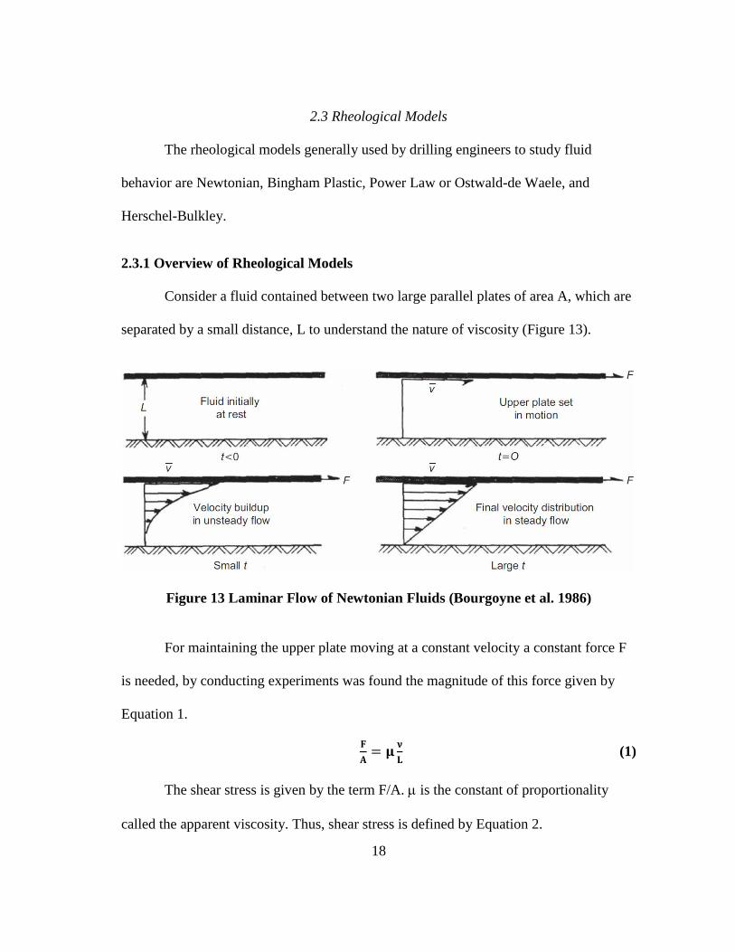
Consider a fluid contained between two large parallel plates of area A, which are
separated by a small distance, L to understand the nature of viscosity (Figure 13).
Figure 13 Laminar Flow of Newtonian Fluids (Bourgoyne et al. 1986)
For maintaining the upper plate moving at a constant velocity a constant force F
is needed, by conducting experiments was found the magnitude of this force given by
Equation 1.
(1)
The shear stress is given by the term F/A. is the constant of proportionality
called the apparent viscosity. Thus, shear stress is defined by Equation 2.
19
(2)
The area of the plate that the fluid is in contact with is represented by A. The
velocity gradient v/L is an expression of the shear rate, Equation 3.
(3)
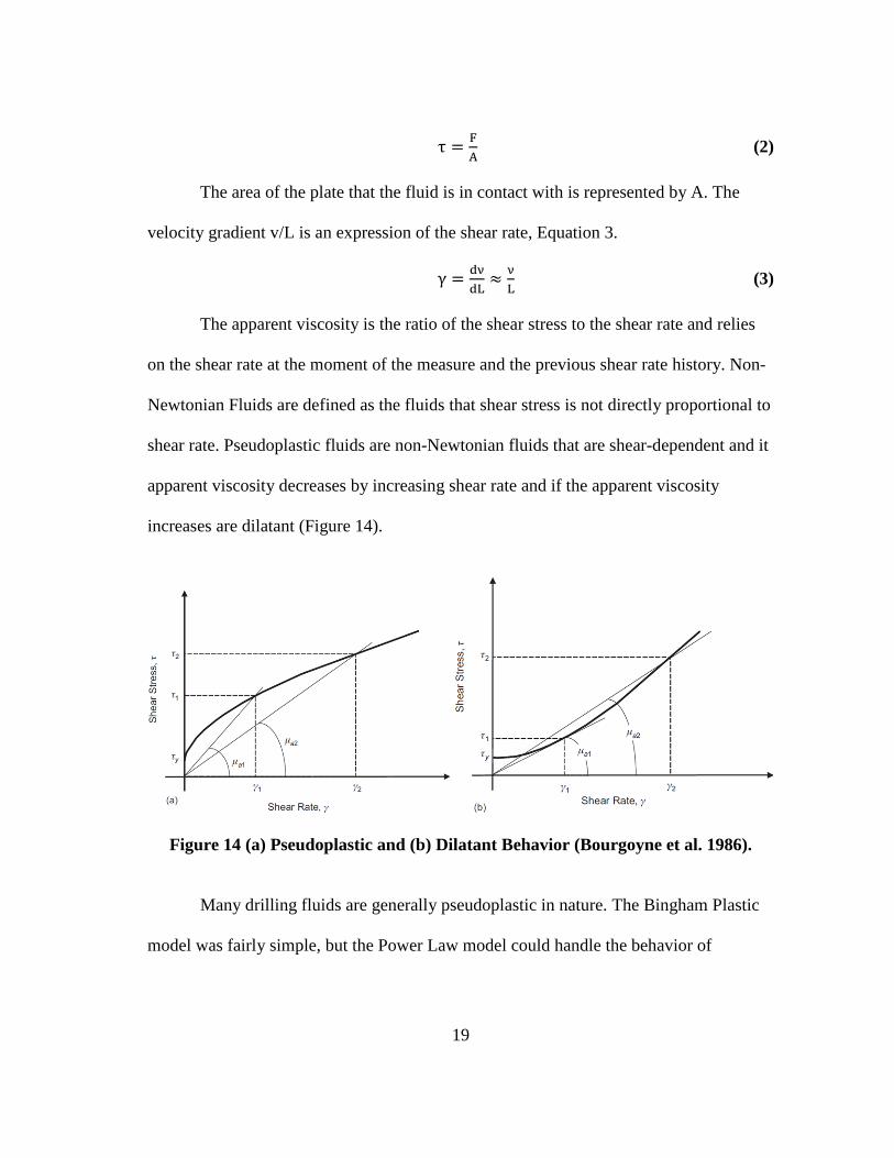
The apparent viscosity is the ratio of the shear stress to the shear rate and relies
on the shear rate at the moment of the measure and the previous shear rate history. Non-
Newtonian Fluids are defined as the fluids that shear stress is not directly proportional to
shear rate. Pseudoplastic fluids are non-Newtonian fluids that are shear-dependent and it
apparent viscosity decreases by increasing shear rate and if the apparent viscosity
increases are dilatant (Figure 14).
Figure 14 (a) Pseudoplastic and (b) Dilatant Behavior (Bourgoyne et al. 1986).
Many drilling fluids are generally pseudoplastic in nature. The Bingham Plastic
model was fairly simple, but the Power Law model could handle the behavior of
20
pseudoplastic drilling fluids better than the Bingham Plastic model, particularly at low
shear rates.
However, a typical behavior of the majority of the drilling fluids used includes a
yield point (YP) (stress required to start fluid moving). The behavior of these fluids,
called pseudoplastic, is characterized by a trend similar to that of pseudoplastic fluids
and by the presence of a finite shear stress at zero shear rate, which is referred to as the
YP. One of the rheological models that fit better this kind of behavior both at low and
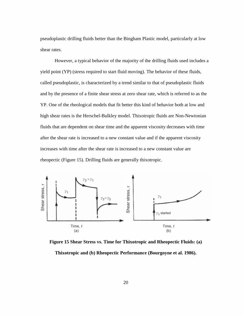
high shear rates is the Herschel-Bulkley model. Thixotropic fluids are Non-Newtonian
fluids that are dependent on shear time and the apparent viscosity decreases with time
after the shear rate is increased to a new constant value and if the apparent viscosity
increases with time after the shear rate is increased to a new constant value are
rheopectic (Figure 15). Drilling fluids are generally thixotropic.
Figure 15 Shear Stress vs. Time for Thixotropic and Rheopectic Fluids: (a)
Thixotropic and (b) Rheopectic Performance (Bourgoyne et al. 1986).
21
At present, the thixotropic performance of drilling fluids is not modeled
mathematically. Nevertheless, drilling fluids are stirred normally prior to measure the
apparent viscosities varying shear rates in order to get steady-state conditions. All the
equations of the models presented are valid only for laminar flow.
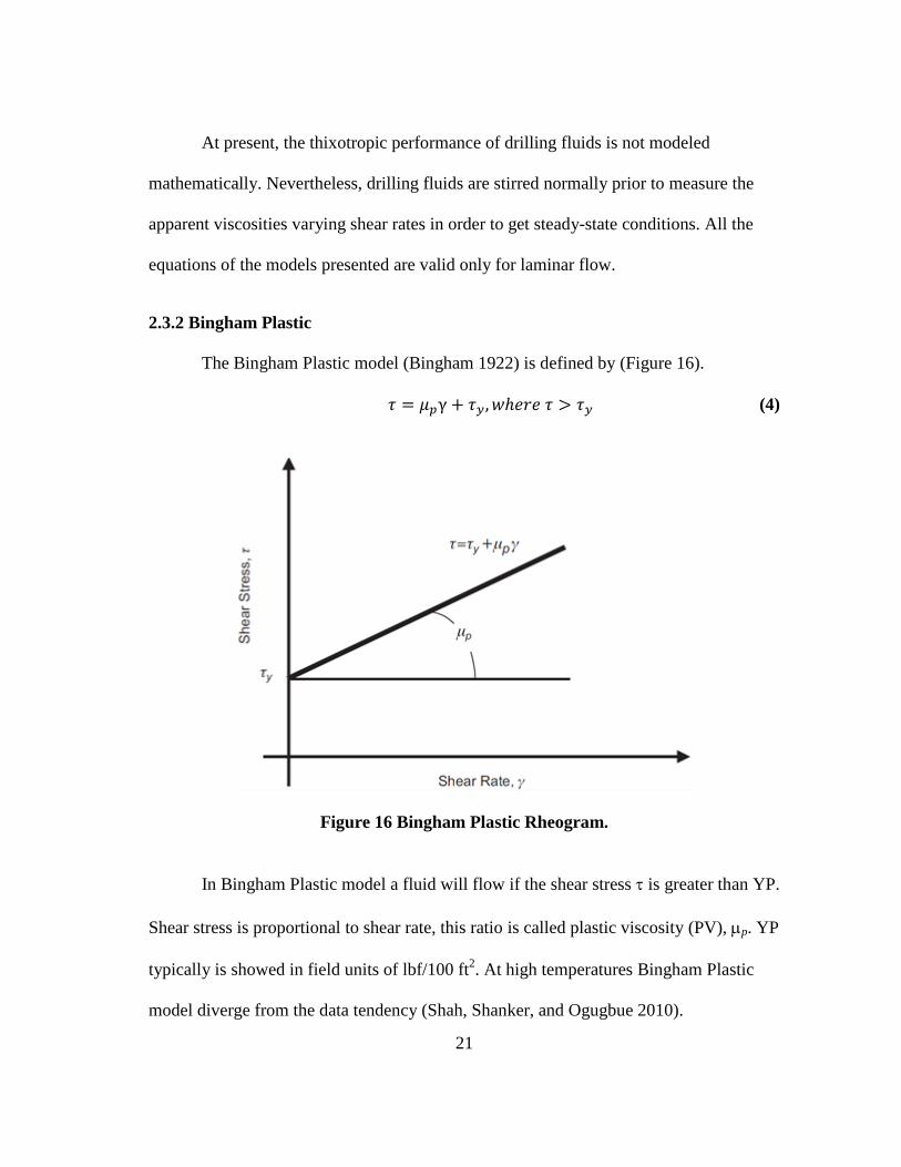
2.3.2 Bingham Plastic
The Bingham Plastic model (Bingham 1922) is defined by (Figure 16).
(4)
Figure 16 Bingham Plastic Rheogram.
In Bingham Plastic model a fluid will flow if the shear stress is greater than YP.
Shear stress is proportional to shear rate, this ratio is called plastic viscosity (PV), p. YP
typically is showed in field units of lbf/100 ft2. At high temperatures Bingham Plastic
model diverge from the data tendency (Shah, Shanker, and Ogugbue 2010).
22
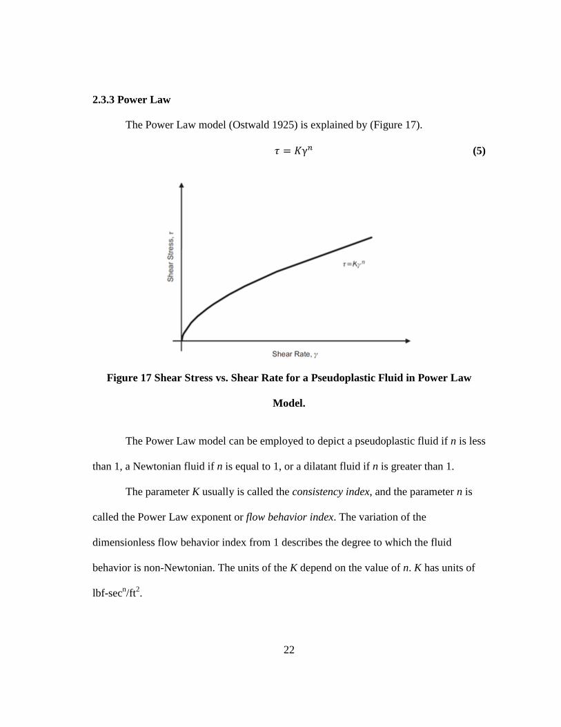
2.3.3 Power Law
The Power Law model (Ostwald 1925) is explained by (Figure 17).
(5)
Figure 17 Shear Stress vs. Shear Rate for a Pseudoplastic Fluid in Power Law
Model.
The Power Law model can be employed to depict a pseudoplastic fluid if n is less
than 1, a Newtonian fluid if n is equal to 1, or a dilatant fluid if n is greater than 1.
The parameter K usually is called the consistency index, and the parameter n is
called the Power Law exponent or flow behavior index. The variation of the
dimensionless flow behavior index from 1 describes the degree to which the fluid
behavior is non-Newtonian. The units of the K depend on the value of n. K has units of
lbf-secn/ft
2.
23
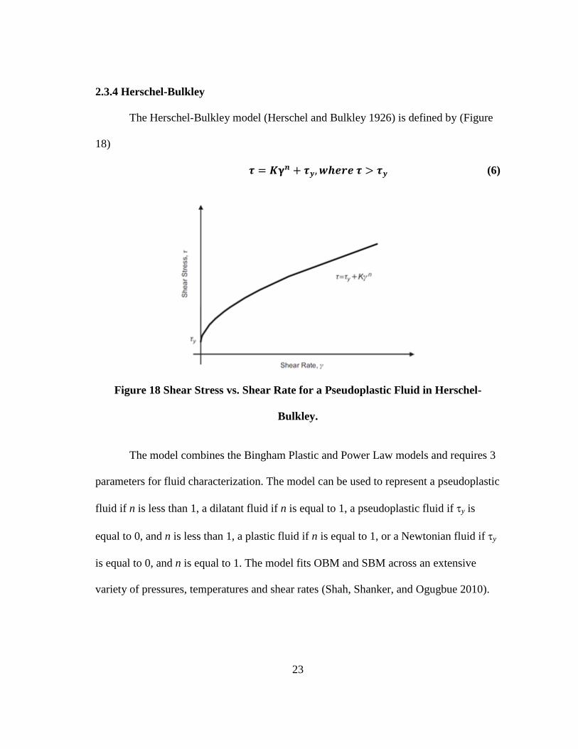
2.3.4 Herschel-Bulkley
The Herschel-Bulkley model (Herschel and Bulkley 1926) is defined by (Figure
18)
(6)
Figure 18 Shear Stress vs. Shear Rate for a Pseudoplastic Fluid in Herschel-
Bulkley.
The model combines the Bingham Plastic and Power Law models and requires 3
parameters for fluid characterization. The model can be used to represent a pseudoplastic
fluid if n is less than 1, a dilatant fluid if n is equal to 1, a pseudoplastic fluid if y is
equal to 0, and n is less than 1, a plastic fluid if n is equal to 1, or a Newtonian fluid if y
is equal to 0, and n is equal to 1. The model fits OBM and SBM across an extensive
variety of pressures, temperatures and shear rates (Shah, Shanker, and Ogugbue 2010).
24
2.3.5 Rheometers and Viscometers
The difference between a viscometer and rheometer is essentially the quality of
components and control capabilities. Basically, a rheometer is more versatile and has a
wider range of applications than a viscometer does.
A rotational viscometer is simple device that rotates a spindle in a single
direction. Most viscometers have mechanical bearings that limit the range of
applications to more viscous materials. A viscometer is a low cost instrument that is
suitable for simple material, process or production tests that require simple flow
measurements. A viscometer is highly suitable for quality control testing and is often
portable so offer the ability to do remote or field testing.
A rotational rheometer allows far significant description of flow and deformation
performance. Rheometers can apply oscillatory motion to the spindles and big step
changes in strain and stress to determine viscoelastic properties as well as flow
properties. Rheometers usually use ultra-low friction air bearings which enable much
greater sensitivity for low viscosity samples to be measured. Rheometers also tend to
offer a wider range of sampling accessories such as temperature control units to study
materials under a wider range of conditions (McDonagh 2010).
Rotational viscometers include Couette-type, parallel disk and cone and plate
viscometers. In Couette-type, rheology can be measured by maintaining constant shear
rate or shear stress (Shah, Shanker, and Ogugbue 2010).
Many of the HPHT Rheometers are design with an ideal pivot without friction
and jewel to give the readings, this condition is not achieved if the test is influenced by
25
pressure, temperature, time of usage and type and content of solids; and hence affecting
the nature of the information created under the most extreme limit of the instrument.
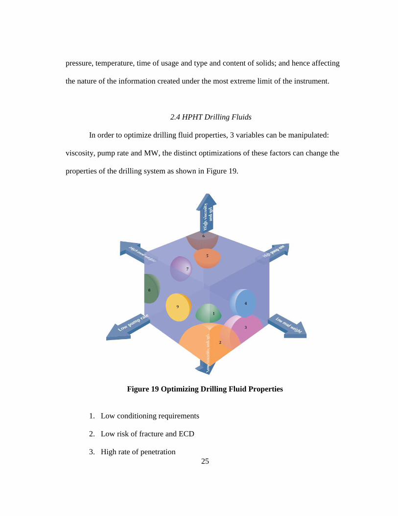
2.4 HPHT Drilling Fluids
In order to optimize drilling fluid properties, 3 variables can be manipulated:
viscosity, pump rate and MW, the distinct optimizations of these factors can change the
properties of the drilling system as shown in Figure 19.
Figure 19 Optimizing Drilling Fluid Properties
1. Low conditioning requirements
2. Low risk of fracture and ECD
3. High rate of penetration
26
4. Minimized differential sticking
5. Minimized Sagging
6. Good hole cleaning
7. Maximum kick prevention
8. Washouts minimized by good hole stability
9. Hydraulic horsepower at bit increased (Adamson et al. 1998)
The success of drilling and its cost depends on 3 factors:
The bit penetrating the rock
The transport of the cuttings to surface and the cleaning of the bit face
The support of the borehole
HPHT Drilling fluids require a good balance of mud properties to avoid oil and
gas surge, kicks, formation damage and other risks. (Amani, Al-Jubouri, and Shadravan
2012)
2.4.1 Functions of Drilling Fluids
The main purposes of the drilling fluid are hole cleaning, formation pressure
control, and carrying cuttings to the surface. According to Mitchell and Miska 2011 can
be categorized as follows:
Cuttings transport
o Clean under the bit
o Transport the cuttings up the borehole
o Release the cuttings at the surface
o Hold cuttings and weighting materials when circulation is interrupted
27
Physicochemical functions
Cooling and lubricating the rotating bit and drill string
Fluid loss control
o Wall the drilled wellbore with an impermeable cake for borehole support
o Reduce adverse and damaging effects on the formation near the wellbore
Subsurface pressure control
Support drillstring and casing weight
Ensure maximum logging information
Transmit hydraulic horsepower to the rotating bit
2.4.2 Drilling-Fluid Categories and Classification
According to the World Oil annual fluid systems classification, there are 10
categories of drilling fluids in use (WorldOil 2015). Six categories include freshwater
systems:
1. Non-dispersed.
2. Dispersed.
3. Calcium-treated.
4. High-performance water-based muds (HPWBM).
5. Low-solids.
6. Polymer/Polyamide (PA)/partially hydrolyzed polyacrylamide (PHPA).
One category covers saltwater systems, two categories include oil- or SBM, and
the last category covers pneumatic (air, mist, foam, gas) ―fluid‖ systems.
28
The principal factors to choose drilling fluids are:
The formation characteristics and properties
The water quality and source for the drilling fluid
The ecological and environmental considerations
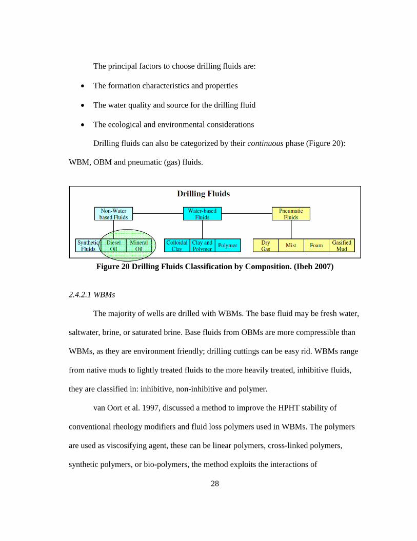
Drilling fluids can also be categorized by their continuous phase (Figure 20):
WBM, OBM and pneumatic (gas) fluids.
Figure 20 Drilling Fluids Classification by Composition. (Ibeh 2007)
2.4.2.1 WBMs
The majority of wells are drilled with WBMs. The base fluid may be fresh water,
saltwater, brine, or saturated brine. Base fluids from OBMs are more compressible than
WBMs, as they are environment friendly; drilling cuttings can be easy rid. WBMs range
from native muds to lightly treated fluids to the more heavily treated, inhibitive fluids,
they are classified in: inhibitive, non-inhibitive and polymer.
van Oort et al. 1997, discussed a method to improve the HPHT stability of
conventional rheology modifiers and fluid loss polymers used in WBMs. The polymers
are used as viscosifying agent, these can be linear polymers, cross-linked polymers,
synthetic polymers, or bio-polymers, the method exploits the interactions of
29
polysaccharides (e.g. xanthan gum, scleroglucan), cellulosics (e.g. carboxymethyl
cellulose (CMC), poly anionic cellulose (PAC)) and starches with polyglycols, he
concluded that polyglycols delay the degradation of the fluid loss polymers at high
temperatures.
Shah, Shanker, and Ogugbue 2010, studied a viscoelastic surfactant (VES)
drilling mud which can re-heal it and reinstate the rheological properties, while VES
based drilling mud is more expensive, it does not need frequent mud conditioning saving
rig time. The cost could be less by blending VES with bio-polymers.
Amani and Al-Jubouri 2012, investigated the effect of HPHT on the rheological
properties of WBM, they concluded:
(1) High YP is gotten by an increment in pressure until 15,000 psi later the YP falls.
At low temperatures the pressure effect on YP is more noticeable.
(2) By increasing temperature PV decreases.
(3) The temperature changing effect is more noticeable than pressure. At
temperatures below 250 °F the pressure effect on PV is more noticeable.
(4) At low temperatures (250 °F) the increment in pressure results in higher
viscosities. Viscosity decreases by increasing temperature until 350 °F then the viscosity
values are small for all distinct rotor speeds. The effect of temperature on viscosity is
more important than pressure.
(5) Gel strength (ability of a fluid to suspend solids) decreases with increasing
temperature until 250 °F afterward generally it increases. The increment in pressure until
30
25,000 psi decrease gel strength then it grows. The pressure effect is more noticeable at
low temperatures (250 °F).
(6) For low density muds, YP is high until 300 °F. Viscosity is high for heavy mud
samples until 400 °F, subsequently the variation between mud weights decrease. For low
density mud, gel strength is normally high. The mud sample degrades at 250 °F.
(7) Rheology of the mud is affected in a complicated way by temperature and
pressure.
(8) Mainly at temperatures lower than the degrade point, a suitable mathematical
approach of the viscosity of WBMs is given by Herschel-Bulkley model.
In WBM systems for HPHT fluids, synthetic polymers are commonly used as
primary viscosifiers and fluid loss agents, such as:
sodium salt of sulfonated acrylamide and vinyl lactam
sodium salt of sulfonated acrylamide, acrylic amide, sodium acrylate and vinyl
lactam
As stated by Hassiba and Amani 2012, Sodium Chloride (NaCl) contaminated
samples had higher shear stress-shear rate curves than WBM; whereas, Potassium
Chloride (KCl) contaminated samples had lower shear stress-shear rate curves than
WBM. These fluids can be polluted during drilling of salt and there is a lot of probability
to find it in deep wells.
Calcium Chloride (CaCl) was found to have a more impact on rheology than
NaCl. The incidence of salt additional lessens the hydration of active clays. Although the
cost of CaCl is more than NaCl per unit (Amani et al. 2015)
31
HPWBM are usually reformulated polymer systems to bring clay and cuttings
inhibition, lubricity and high ROP, shale stability, by the time that downhole torque and
bit balling problems are minimized. In order to reduce pore pressure transmission
HPWBM use products to stabilize the borehole similar to OBMs (WorldOil 2015).
According to Ofei and Al Bendary 2016, Potassium formate brine (KCHO2) is
usually used to stabilize the drilling fluid’s performance under HPHT conditions as it
helps in decreasing the flocculation of rheological properties of WBM under extreme
temperature including the degradation of their rheological properties.
2.4.2.2 OBMs
The drilling efficiency of an OBM system can save time required to drill the
well. These fluid systems are also subject to disposal regulations because of their
toxicity. Mineral oil formulations are considered less toxic than diesel-based fluids, but
not a suitable alternative where ―greener‖ SBMs are available. The use of diesel or
mineral OBMs is absolutely prohibited in some areas. The oil/water ratios typically
range from 90:10 to 60:40. Generally, the higher the percentage of water, the thicker the
drilling fluid is. High salinity levels in the water phase dehydrate and harden reactive
shales by imposing osmotic pressures.
As stated by Ibeh 2007, many factors affect fluid rheology including pressure,
temperature, shear history, arrangement and the electrochemical character of the
segments and of the persistent liquid stage, and can be synthetized as follows:
Physical. The pressure effect is predicted to be bigger with OBM due to the oil
phase compressibility.
32
Electrochemical. The ionic activity of any electrolyte and the solubility of any
soluble salt present in the fluid increase while temperature increases.
Chemical. Hydroxides react with clay minerals at temperatures above 200 °F,
this produce a change of the structure and of the rheological properties.
According to Ibeh 2007, at constant temperature the YP values are less uniform,
but they generally increase with increasing pressure or decreasing temperature. At
constant pressure there was a steady decline in viscosity with increasing in temperature
up to 450 °F, where there is an increment due to thermal degradation that produces a
change in the composition of the fluid. The effect of pressure is strongest at low
temperature. At constant shear rate it exists the term ―two-way‖ heating and cooling
down. Ibeh 2007, also concluded that there is a linear relation between pressure and
viscosity whiles an exponential relation for temperature, as well that the temperature
effects on viscosity of the OBMs are more noticeable at high pressures above 20,000 psi,
while pressure effects overcome at low temperatures below 350 °F and the thermal
degradation occurs quicker at lower pressures below 10,000 psi than at higher pressures
if the shear history is the same.
OBM Advantages:
Most of OBMs are stable until 450 °F as defined by rheology and fluid loss.
High lubricity, used to drill through most troublesome shale formations due to
the inhibition and temperature stability (Ibeh 2007).
Provides better gauge hole and not to leach out salt by faster penetration rates.
33
Control fluid loss excellent, no shale swelling, good cutting carrying ability and
adequate lubrication to drill bits (Shah, Shanker, and Ogugbue 2010).
By using palm oil as an alternative of diesel can be more environmentally
friendly (Shah, Shanker, and Ogugbue 2010).
Thin filter cake (De Stefano, Stamatakis, and Young 2012).
Resistant to salt, anhydrite, H2S and CO2. (Amani, Al-Jubouri, and Shadravan
2012)
Reduces differential sticking risk.
Allow low pore pressure formations drilling.
Exceptional corrosion protection.
Last long time.
OBM Disadvantages:
Makes more difficult the detection of a kick, because of solubility of gas in the
base fluid (Adamson et al. 1998).
The thermal expansion of OBM is bigger than WBM, generating pressure in the
annulus (Bland et al. 2006).
Reduced rheology and filtration control when exposed to temperatures higher
than 300 °F for long periods of time (Ibeh 2007).
Due to oil wet surfaces poor bonding between formation and cement.
Deficient filter cake removal and possible environmental risks, like seepage into
aquifers and causing contamination (Shah, Shanker, and Ogugbue 2010).
High cost lost circulation problems.
34
Emulsifiers used in OBMs can change the rock wettability to oil-wet (Amani, Al-
Jubouri, and Shadravan 2012).
The use of oil resistant rubber is needed; due to the circulating system rubber
parts can be damaged.
Fire risks due to low flash points of vapors.
To diminish OBM loss supplementary rig equipment and modifications are
needed (Abduo et al. 2015).
Amani 2012, drawn the subsequent observations based on rheology tests at
HPHT conditions on two OBMs, one regular and the other HPHT resistant. By
increasing temperature; viscosity, gel strength and YP decrease (before the sample
degrades, for regular OBM). This performance was consequence of the thermal
degradation of the polymers, solids, and other components of the sample and the
development of the atomic separations that low its viscosity, gel strength and YP.
Besides, it was inferred that YP and viscosity increase with pressure. At low
temperatures (below degrade point, for regular OBM) pressure effect on these
parameters, is more noticeable. The viscosity, YP, and gel strength was directly
proportional to pressure and inversely proportional to temperature. The temperature and
pressure dependence of viscosity was exponential. YP is used to analyze the capability
of a mud to lift cuttings from the annulus. If the YP is high it means a non-Newtonian
fluid, which carries cuttings better than a low YP fluid, a flocculant or a freshly
dispersed clay, like lime increase YP and is decreased by the addition of deflocculant to
35
a clay-based mud. The OBM sample with regular formulation degraded at 400 °F and
the HPHT sample resisted.
2.4.2.2.1 All-Oil Muds
Drilling fluids formulated with diesel- or synthetic-based oil and no water phase
are used to drill highly variable salinity formation water intervals of long shale (Mitchell
and Miska 2011).
In order to control viscosity and fluid loss asphaltic type materials are needed.
An invert emulsion is required if the water turn into a polluting effect. Mud solids can
become water wet and cause stability problems if water is not emulsified fast. Mud can
be lost if the water wet solids blind the screens of the shakers (Amani, Al-Jubouri, and
Shadravan 2012).
2.4.2.2.2 SBMs
The term ―synthetic‖ is used for non-aqueous fluids formulated with the reaction
of fundamental organic building blocks, such as methane or ethylene. Typically, the high
salinity water phase of an invert emulsion or SBM aids to stabilize reactive shale and
prevent swelling.
SBMs were developed to provide the highly regarded drilling-performance
characteristics of conventional OBMs while significantly reducing the toxicity of the
base fluid, due to the aromatic content is low. Consequently, SBMs are used almost
universally offshore. The cost-per-barrel for an SBM is considerably higher than that of
an equivalent-density WBM, but because synthetics facilitate high ROPs and minimize
36
wellbore instability problems, the overall well-construction costs are generally less,
unless there is a catastrophic lost-circulation occurrence.
An example of synthetic fluid is an ester formulated with an alcohol and a natural
fatty acid. Other synthetic fluids are alkylbenzenes, acetals and an assortment of
aliphatic hydrocarbons derived from ethylene. The typical synthetic fluid is an internal
olefin with a carbon chain length of C16-C18.
In 2002, an SBM formulated with an ester/IO blend became widely used,
especially in deepwater operations where temperatures range from 40 to 350 °F on a
given well, the fluid contained no commercial clays or treated lignites; rheological and
fluid loss control properties were maintained with specially designed fatty acids and
surfactants, the system provided stable viscosity and flat rheological properties over an
extensive variety of temperatures.
2.4.2.2.3 Emulsion-Based Drilling Fluids (EBFs)
The external phase of an EBF is water or brine and the internal phase is oil,
synthetic hydrocarbons replace oil as an internal phase, in order to make the two phases
miscible a surfactant is used, this fluid is cheaper than OBM, however more expensive
than WBM, furthermore can be safely disposed of and is environmental friendly (Shah,
Shanker, and Ogugbue 2010).
In EBF gel strengths develop quickly, but are extremely shear-sensitive; as a
result, pressures related to breaking circulation, tripping or running casing, cementing,
and ECD are significantly lower than pressures that occur with conventional invert
emulsion fluids. Lost circulation incidents appear to occur less frequently and with a
37
lesser degree of severity where EBFs are used. The EBF performs well from an
environmental perspective and has met or surpassed stringent oil-retained-on cuttings
regulations governing cuttings discharge in the GOM. The EBF is highly water and
solids tolerant and responds rapidly to treatment.
2.4.2.2.4 Invert Emulsion Drilling Fluids
Invert emulsion fluids consist of an aqueous fluid emulsified into a non-aqueous
phase. An emulsion is created between two incompatible liquids by reducing the
interfacial surface tension of one liquid with an emulsifier, or surfactant, to allow that
liquid to create a stable dispersion of fine droplets in the other liquid. The droplet size is
small when interfacial tension is low; typically the more stable the emulsion will be (De
Stefano, Stamatakis, and Young 2012). Invert emulsions are inhibitive, resistant to
contaminants, stable at HPHT, lubricious, and noncorrosive. Onshore, they are the fluids
of choice for drilling troublesome shale sections, extended-reach wells that would be
otherwise prone to pipe-sticking problems, and dangerous HPHT H2S wells. The basic
components of an invert-emulsion fluid (Figure 21) include an oleaginous liquid
(synthetic fluids, diesel or mineral oil, which serves as the continuous phase); brine
(usually CaCl that serves as the discontinuous phase), emulsifiers, oil-wetting agents,
organophilic clay, filtration-control additives, and slaked lime. The primary emulsifiers
are calcium-based soaps. Secondary emulsifiers enhance temperature stability and are
tall oils (Mitchell and Miska 2011).
38
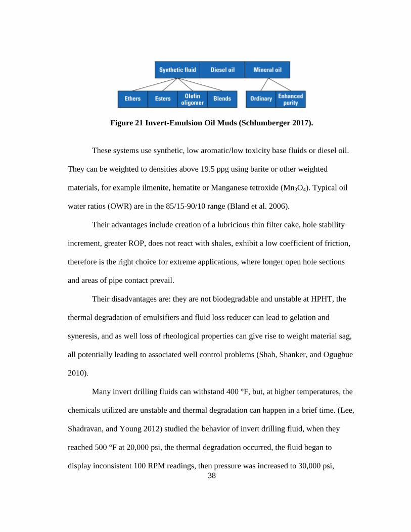
Figure 21 Invert-Emulsion Oil Muds (Schlumberger 2017).
These systems use synthetic, low aromatic/low toxicity base fluids or diesel oil.
They can be weighted to densities above 19.5 ppg using barite or other weighted
materials, for example ilmenite, hematite or Manganese tetroxide (Mn3O4). Typical oil
water ratios (OWR) are in the 85/15-90/10 range (Bland et al. 2006).
Their advantages include creation of a lubricious thin filter cake, hole stability
increment, greater ROP, does not react with shales, exhibit a low coefficient of friction,
therefore is the right choice for extreme applications, where longer open hole sections
and areas of pipe contact prevail.
Their disadvantages are: they are not biodegradable and unstable at HPHT, the
thermal degradation of emulsifiers and fluid loss reducer can lead to gelation and
syneresis, and as well loss of rheological properties can give rise to weight material sag,
all potentially leading to associated well control problems (Shah, Shanker, and Ogugbue
2010).
Many invert drilling fluids can withstand 400 °F, but, at higher temperatures, the
chemicals utilized are unstable and thermal degradation can happen in a brief time. (Lee,
Shadravan, and Young 2012) studied the behavior of invert drilling fluid, when they
reached 500 °F at 20,000 psi, the thermal degradation occurred, the fluid began to
display inconsistent 100 RPM readings, then pressure was increased to 30,000 psi,
39
causing a considerable variation in the dial readings, since the fluid was so viscous.
After the cell was disassembled, it was noticed that the fluid had separated into two
phases with a clear oil phase on the top and a thick paste at the bottom of the cell. The
xHPHT invert fluid holds products specially designed to withstand 600 °F, it had a good
thermal stability as it exhibited very stable properties after heat aging. The most
common emulsifiers for invert emulsion drilling fluids are surfactants distinguished to
have functional groups that confer a polarity within the molecule, such as fatty acids,
alcohols and amines (Young, De Stefano, and Lee 2012).
Almost all amido-amine emulsifiers are not capable to withstand temperatures
above 450 °F, because they started to decompose, releasing ammonia and deteriorating
fluid properties, for overcoming this challenge a emulsifier has been added to keep
emulsion and fluid property stability, but this increment the cost.
The surfactant technologies provide a non-nitrogen based chemistry invert
emulsifier that is capable to maintain stability of system properties and maintenance of
oil wetting on prolonged exposure to temperatures in the 475-600 °F range (Young, De
Stefano, and Lee 2012).
Invert emulsions are formulated to contain as much as 60 % of water; this is an
integral part of the invert emulsion and can include a salt such as CaCl or NaCl. In order
to tightly emulsify the water as the internal phase and prevent the water from breaking
out and coalescing into larger water droplets, special emulsifiers are used.
Relaxed invert emulsion is when the fluid loss control of the system is relaxed
with improvement in drilling rates; this uses more emulsifier than a regular invert
40
emulsion, (Amani, Al-Jubouri, and Shadravan 2012). Relaxed OBMs are formulated
without filtration-control additives and have a loose emulsion.
2.4.2.3 Formate Brines
The birth of formate brines was in the early 1990’s by Shell, the ideal solution
was developing one fluid that:
reduced hydraulic flow resistance
eliminated solids sag
did not solubilize hydrocarbon gases
was not destabilized by the influx of reservoir gases
reduced localized or pitting corrosion by acid gases
eradicated stress corrosion cracking
avoided corrosion inhibitors usage
avoided causing formation damage
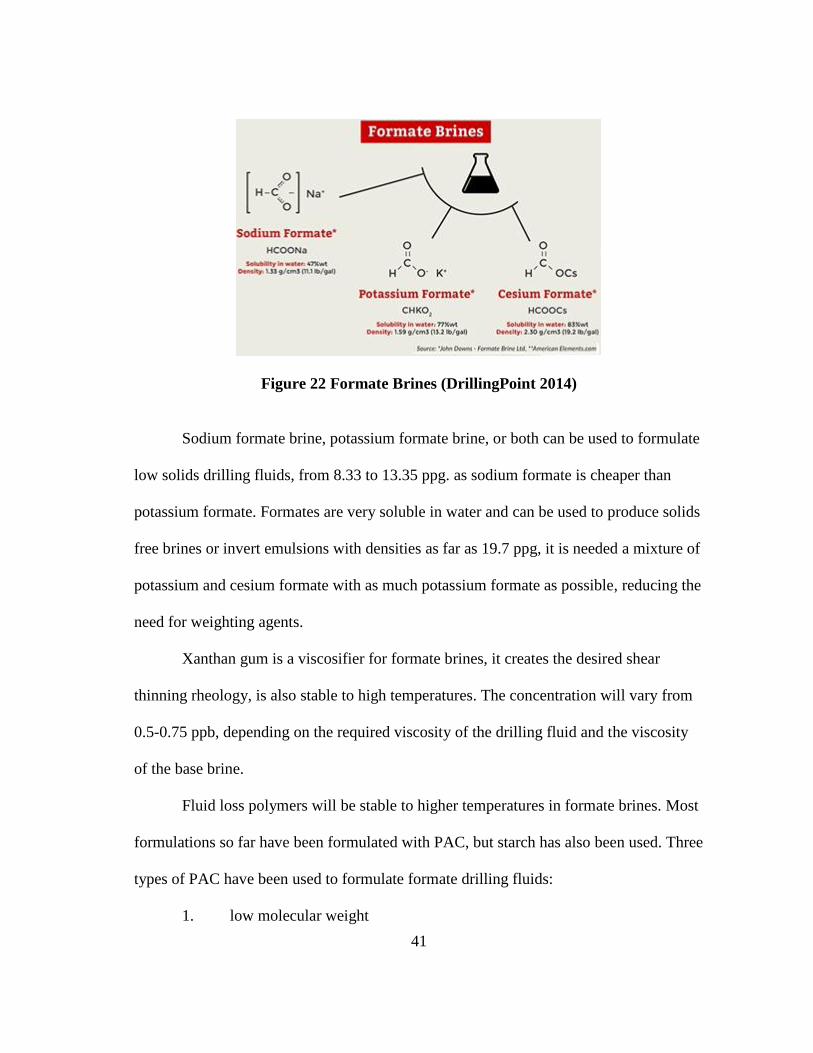
Formate salts derived from formic acid (HCOOH), and formulate by the
incorporation of formate salts to fresh water, these format salts can be: sodium formate
(HCOONa), potassium formate (CHKO2) or anhydrous cesium formate (HCOOCs)
(Howard 1995) (Figure 22).
41
Figure 22 Formate Brines (DrillingPoint 2014)
Sodium formate brine, potassium formate brine, or both can be used to formulate
low solids drilling fluids, from 8.33 to 13.35 ppg. as sodium formate is cheaper than
potassium formate. Formates are very soluble in water and can be used to produce solids
free brines or invert emulsions with densities as far as 19.7 ppg, it is needed a mixture of
potassium and cesium formate with as much potassium formate as possible, reducing the
need for weighting agents.
Xanthan gum is a viscosifier for formate brines, it creates the desired shear
thinning rheology, is also stable to high temperatures. The concentration will vary from
0.5-0.75 ppb, depending on the required viscosity of the drilling fluid and the viscosity
of the base brine.
Fluid loss polymers will be stable to higher temperatures in formate brines. Most
formulations so far have been formulated with PAC, but starch has also been used. Three
types of PAC have been used to formulate formate drilling fluids:
1. low molecular weight
42
2. extremely low molecular weight
3. ultra-low molecular weight
Although the formate drilling fluids are often referred to as "solids free", this is
not entirely true, as a minimum amount of solids is required for the formation of a filter
cake. The ideal filter cake material in a formate drilling fluid is calcium carbonate
(CaCO3) (chalk), which can easily be removed with acid. An amount of about 10 to 20
ppb is sufficient to create a thin and very efficient filter cake.
According to Howard 1995, 4 minerals can be used as weighting materials:
Chalk (CaCO3), Siderite (FeCO3), Manganese tetroxide (Mn3O4) and Hematite (Fe2O3).
The advantages of formate brines are:
Formation damage is minimal
Better thermal stability
Elimination of barite sag problems
Minimize hydraulic flow resistance
o Low ECDs
o Low swab and surge pressures
o Better power transmission to motors and bits
Low gas solvency
o Better kick detection and well control
o Faster flow-checks
Low probability of differential sticking
Reduced torque and drag
43
Naturally lubricating
Hydrate formation inhibition
Non-hazardous
Low corrosion rates
Compatibility with elastomers
No stress corrosion cracking
Environmentally friendly and biodegradable (Downs 2006)
Due to high viscosity of filtrate and low water activity excellent shale
stabilization.
High formation strength and wellbore stability.
The disadvantages are: fluid loss in some cases is ten times more than a typical
OBM, they are more expensive and made log analysis more complex (Ibeh 2007).
Formate muds are commonly protected with a carbonate salt, due to halides are
very corrosive at high temperatures and constitute an environmental risk. In formate
solutions corrosion rates are low, providing an alkaline pH. Formates are easily
biodegradable and can be used without problems in environmentally sensitive areas.
Low solids concentrations frequently enhance ROP and let good rheological properties
control. Additionally formate brines have low water activity; hence, they decrease clay
hydration and encourage borehole stability throughout osmosis (DeBruijn et al. 2008).
Recent research done by van Oort et al. 2015 in large scale drilling machines has
shown that the ROP in formate brines can be up to 50 % higher than ROP in OBMs. To
save cost a mixture should always be made with as much sodium formate as possible,
44
also can be formulated on pure potassium formate brine weighted to required density
with solid weight material. When low rheology is desired is better to choose a slightly
low brine concentration, and use some additional weight material. A cube of formate is
360 % more expensive compared to invert emulsion mud. By using formate, costs
decreased by 27 % per lateral meter drilled for the entire well. The demand for formate
brines has been growing 30 % per annum over the past decade.
2.4.3 Drilling Fluids of Ultra HPHT Well on the GOM Mexican Side
When higher temperatures to 204 °C (400 °F) are showed, the drilling mud,
regardless of the base (oil or synthetic), does get a bit more than 40 % solids in its
composition. To remain stable and functional, it requires constant dynamic conditions
downhole, because the high temperature present in the drilled area affects and changes
the rheological properties to a point of null effectiveness; leading to hole instability
problems and influences of abnormal pressure zones, in this way organophilic clays and
emulsifiers of latest generation are used, due to it increases thermal stability and reduces
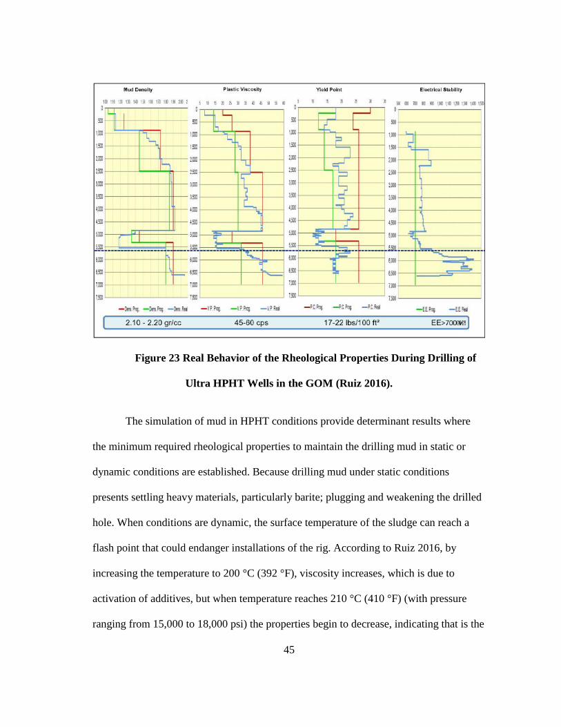
drilling mud filtrate (Figure 23).
45
Figure 23 Real Behavior of the Rheological Properties During Drilling of
Ultra HPHT Wells in the GOM (Ruiz 2016).
The simulation of mud in HPHT conditions provide determinant results where
the minimum required rheological properties to maintain the drilling mud in static or
dynamic conditions are established. Because drilling mud under static conditions
presents settling heavy materials, particularly barite; plugging and weakening the drilled
hole. When conditions are dynamic, the surface temperature of the sludge can reach a
flash point that could endanger installations of the rig. According to Ruiz 2016, by
increasing the temperature to 200 °C (392 °F), viscosity increases, which is due to
activation of additives, but when temperature reaches 210 °C (410 °F) (with pressure
ranging from 15,000 to 18,000 psi) the properties begin to decrease, indicating that is the
46
point where the additives lose performance and efficiency. Laboratory results not only
determine the minimum required rheological properties, also provide valuable
information to the design and optimization of hydraulic of the well with cost models,
time traffic cycles and management of annular velocities, counteracting the effects by
the high temperature in drilling mud as well as prolonged periods of preparation and
conditioning. The design of the drilling mud to Ultra HPHT areas involves supplying of
new materials in short periods through logistics and a large storage capacity, making
sure it is in good condition. One of the best practices applied in the newly drilled wells
that have substantial savings for Ultra HPHT wells is to include a support mud ship and
a platform with plenty of dam capacity to pump new mud according to the time
established by a risk analysis and laboratory simulations.
47
CHAPTER III
EQUIPMENT AND METHODOLOGY
3.1 Model 7600 HPHT Viscometer
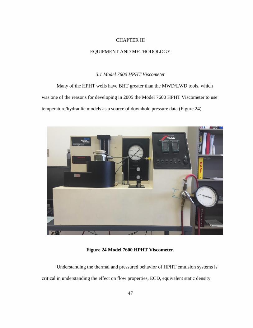
Many of the HPHT wells have BHT greater than the MWD/LWD tools, which
was one of the reasons for developing in 2005 the Model 7600 HPHT Viscometer to use
temperature/hydraulic models as a source of downhole pressure data (Figure 24).
Figure 24 Model 7600 HPHT Viscometer.
Understanding the thermal and pressured behavior of HPHT emulsion systems is
critical in understanding the effect on flow properties, ECD, equivalent static density
48
(ESD), and kick detection. As Baker Hughes Drilling Fluids (BHDF) developed HPHT
fluid systems for more extreme environments, the need to test them posed the parallel
challenge of designing a HPHT viscometer. The design criteria put forth by the
technology team included a working temperature of 600 °F (316 °C), working pressure
of 40,000 psi (276 MPa), the drive magnets are above the fluid sample to allow accurate
viscosity measurements on fluids containing ferromagnetic materials and to reduce the
chance of over-heating the magnets. The opportunity to achieve the criterion of perfectly
steady, laminar flow is unlikely for high density, non-Newtonian high solids-content
fluids used in HPHT viscometers (Gusler et al. 2006).
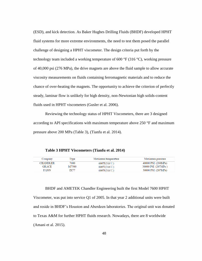
Reviewing the technology status of HPHT Viscometers, there are 3 designed
according to API specifications with maximum temperature above 250 °F and maximum
pressure above 200 MPa (Table 3), (Tianfu et al. 2014).
Table 3 HPHT Viscometers (Tianfu et al. 2014)
BHDF and AMETEK Chandler Engineering built the first Model 7600 HPHT
Viscometer, was put into service Q1 of 2005. In that year 2 additional units were built
and reside in BHDF’s Houston and Aberdeen laboratories. The original unit was donated
to Texas A&M for further HPHT fluids research. Nowadays, there are 8 worldwide
(Amani et al. 2015).
49
This is a Couette viscometer with a concentric cylinder that uses a rotor and bob
geometry, also compliance with the necessities of ISO and API standards to measure the
viscosity of HPHT fluids.
For this viscometer, the shear stress (torque) created between the bob and rotor is
measured using a precision torsion spring and high resolution encoder. Known sample
shear rates are created between the bob and the rotor using precision defined bob/rotor
geometry and a stepper motor subsystem. Suspended solids in the sample are circulated
during the test using a helical screw on the outside diameter of the rotor.
Features and Benefits:
External digital torque measurement
Separation zone between sample and oil
Corrosion resistant steel super-alloys with high strength
Programmable Pressure and Temperature Controllers
Shear stress range: 5.1-1533 dyne/cm2
Shear stress accuracy: ±0.50 %
Shear rate range from 1.7 to 1533 sec-1
(1 to 900 RPM)
Viscosity range: 2 cp at 600 RPM and 300 cp at 300 RPM.
3.2 Experimental Setup
The Model 7600 HPHT Viscometer consists of 3 main parts: top cap on the top
part, top plug in the middle and vessel at the bottom. The bob and rotor cylinders are
located inside the vessel where the fluid sample is, its capacity is 195 ml. The rotational
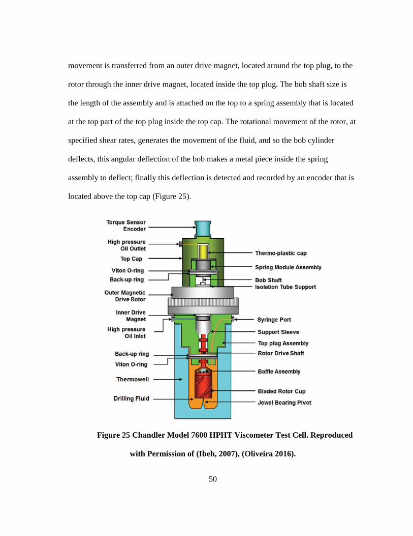
50
movement is transferred from an outer drive magnet, located around the top plug, to the
rotor through the inner drive magnet, located inside the top plug. The bob shaft size is
the length of the assembly and is attached on the top to a spring assembly that is located
at the top part of the top plug inside the top cap. The rotational movement of the rotor, at
specified shear rates, generates the movement of the fluid, and so the bob cylinder
deflects, this angular deflection of the bob makes a metal piece inside the spring
assembly to deflect; finally this deflection is detected and recorded by an encoder that is
located above the top cap (Figure 25).
Figure 25 Chandler Model 7600 HPHT Viscometer Test Cell. Reproduced
with Permission of (Ibeh, 2007), (Oliveira 2016).
51
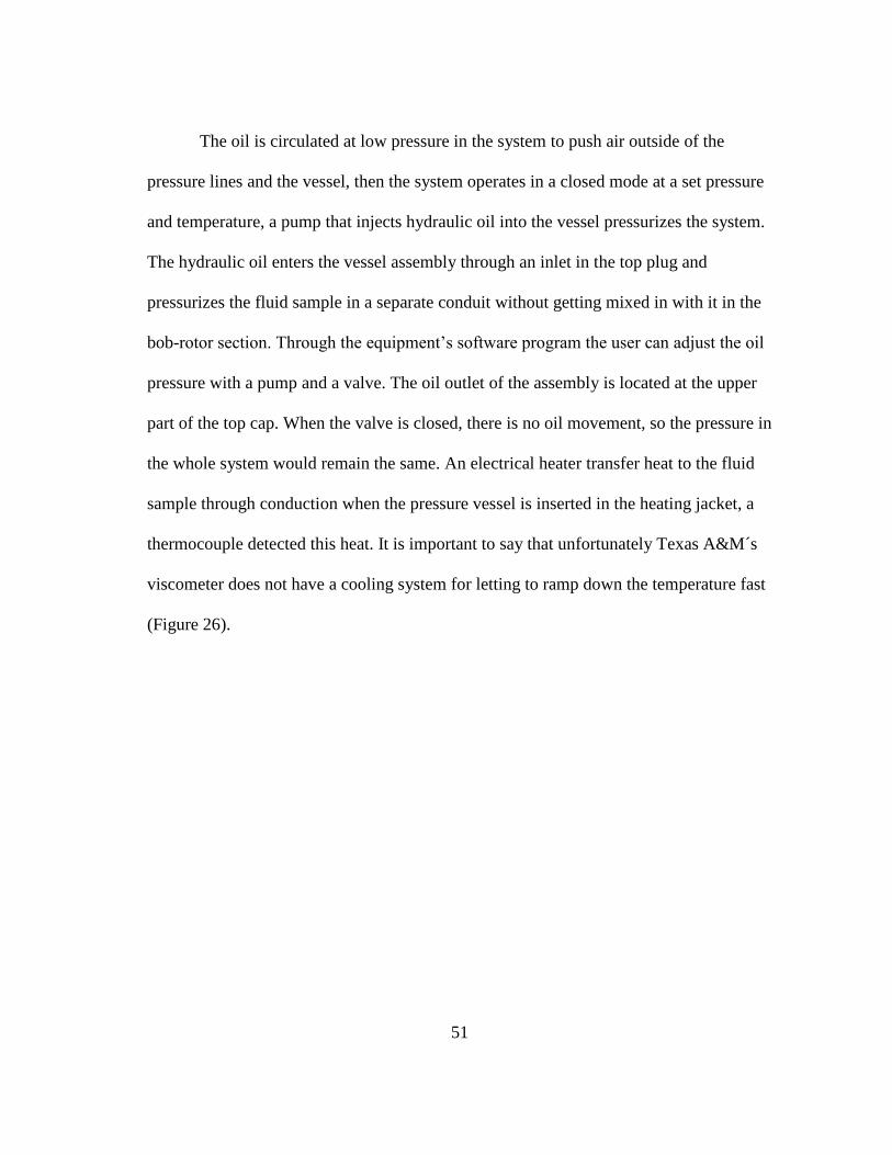
The oil is circulated at low pressure in the system to push air outside of the
pressure lines and the vessel, then the system operates in a closed mode at a set pressure
and temperature, a pump that injects hydraulic oil into the vessel pressurizes the system.
The hydraulic oil enters the vessel assembly through an inlet in the top plug and
pressurizes the fluid sample in a separate conduit without getting mixed in with it in the
bob-rotor section. Through the equipment’s software program the user can adjust the oil
pressure with a pump and a valve. The oil outlet of the assembly is located at the upper
part of the top cap. When the valve is closed, there is no oil movement, so the pressure in
the whole system would remain the same. An electrical heater transfer heat to the fluid
sample through conduction when the pressure vessel is inserted in the heating jacket, a
thermocouple detected this heat. It is important to say that unfortunately Texas A&M´s
viscometer does not have a cooling system for letting to ramp down the temperature fast
(Figure 26).
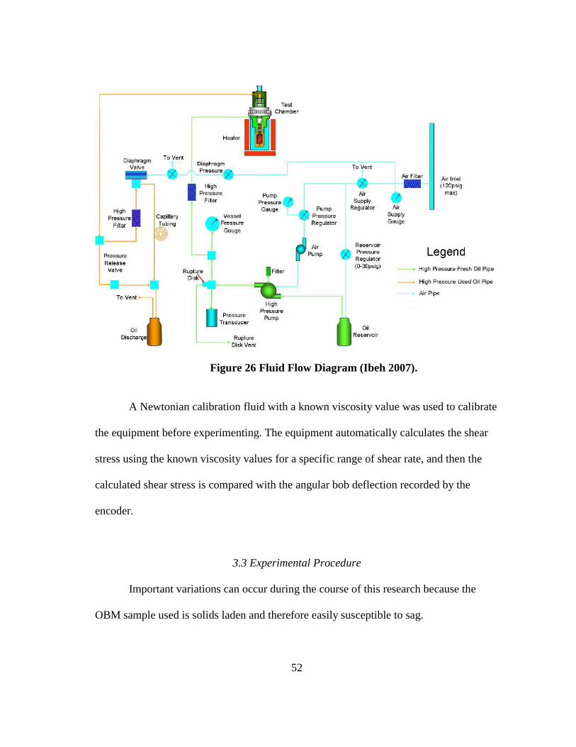
52
Figure 26 Fluid Flow Diagram (Ibeh 2007).
A Newtonian calibration fluid with a known viscosity value was used to calibrate
the equipment before experimenting. The equipment automatically calculates the shear
stress using the known viscosity values for a specific range of shear rate, and then the
calculated shear stress is compared with the angular bob deflection recorded by the
encoder.
3.3 Experimental Procedure
Important variations can occur during the course of this research because the
OBM sample used is solids laden and therefore easily susceptible to sag.
53
3.3.1 Fluid Type
One OBM formulation was used during this research, it will be referred to as
―Sample‖, below is a brief description of it.
3.3.2 Sample
It was brought from Ciudad del Carmen, Campeche, Mexico. This sample was
prepared by M-I-SWACO to Pemex. It mud weight was measured using a mud balance
getting the value of 13.5 ppg. The base oil was diesel and it was weighted with barite.
The sample was obtained from the field in Offshore Mexico.
3.3.3 Fluid Preparation
The following actions were done prior to test the sample with the HPHT
viscometer:
1. The fluid was blended with a pallet then with a mixer at 70 RPM for less than
5 min. to guarantee a homogeneous mixture.
2. Part of the sample was poured out to fill the 100 mL test tube and poured into
the Erlenmeyer flask; the remaining 95 mL were measured and poured in the same way.
3. Using a hose from the adapter plug into an Erlenmeyer flask and pressurized
the flask with a blue line of air connected to the flask adapter, the air supply was opened,
also the valve that is in the front of the blue air line near to the manometer, next the
sample was pumped into the cell, finally 195 mL of mud sample were injected.
54
3.4 Experimental Schedule
This viscometer as an automated unit needs initial programming of an operating
schedule for the whole experimental cycle. The schedule contains magnitude and
duration of each viscometer experimental condition in which viscosity is recorded in a
special order automatically. Extensive initial tests were conducted to obtain a steady
state operating schedule to obtain repeatable experiments (Anoop et al. 2014).
The test schedule used was test_pressures_Pedro_e_Rafael_9.sch, it is described
by the succeeding steps: the pressure is raised to 10,000 psi later decreases to 5,000 psi
and 1 hr. is waited, afterward 7 stages are run with temperature increments of 50 ºF from
100 to 400 °F (above this temperature smoke starts to appear), during every constant
temperature stage the pressure is increased by 5,000 psi from 5,000 to 35,000 psi
(38,000 psi is the highest pressure achieved), in each pressure step the shear rate first is
raised to 100 RPM next to 600 RPM, subsequently decreases to 300, 200, 100, 60, 6, 3
RPM for taking dial reading, viscosity and shear stress values, after that, 10 sec and 10
min gel strengths are taken at 3 RPM.
The software this viscometer uses is Rheo 7000, with this all the orders are sent
automatically to the HPHT Viscometer and the data is recorded. It uses the following
equations to calculate shear stress, shear rate, and viscosity:
(7)
(8)
(9)
55
(10)
(11)
(12)
(13)
where,
M = Torque on Bob shaft (dyne-cm)
L = Bob Height, cm
w = Angular Velocity, sec-1
Ri = Bob Radius, cm
Ro = Rotor Radius, cm
PV = Plastic Viscosity, cP
YP = Yield Point, lbf/100ft2
Time = sec
Temperature = °F
Pressure = psi
Angle = degrees
Shear Stress = degrees (for a given spring constant) and dyne/cm2
Spring Constant = dyne-cm/degree
Viscosity = cP
Gel Strength = lbf/100ft2
Shear Rate = sec-1
Motor Speed = RPM
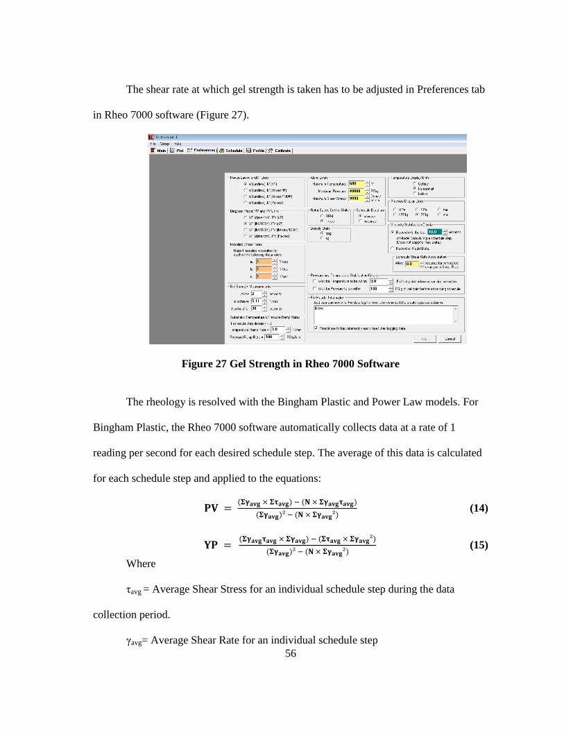
56
The shear rate at which gel strength is taken has to be adjusted in Preferences tab
in Rheo 7000 software (Figure 27).
Figure 27 Gel Strength in Rheo 7000 Software
The rheology is resolved with the Bingham Plastic and Power Law models. For
Bingham Plastic, the Rheo 7000 software automatically collects data at a rate of 1
reading per second for each desired schedule step. The average of this data is calculated
for each schedule step and applied to the equations:
(14)
(15)
Where
τavg = Average Shear Stress for an individual schedule step during the data
collection period.
γavg= Average Shear Rate for an individual schedule step
57
N= Number of schedule steps
The accuracy of the model is expressed as:
(∑
∑
(∑ )
) (16)
Where εi represents the difference between the measured shear stress and the
calculated shear stress using the Bingham Plastic equation for schedule step i.
In a similar way for Power Law model, the average of this data is calculated for
each schedule step and applied to the equations:
( ) ( )
( ) ( )
(17)
(18)
The accuracy of the model is expressed as:
(
( )
) 19
Finally the test results are analyzed by doing conclusions and recommendations,
if something is wrong, it is necessary to identify the causes and where is the problem
located to recalibrate the damaged viscometer´s parts. (Ibeh 2007) did a workflow
process for a typical viscometer test (Figure 28).
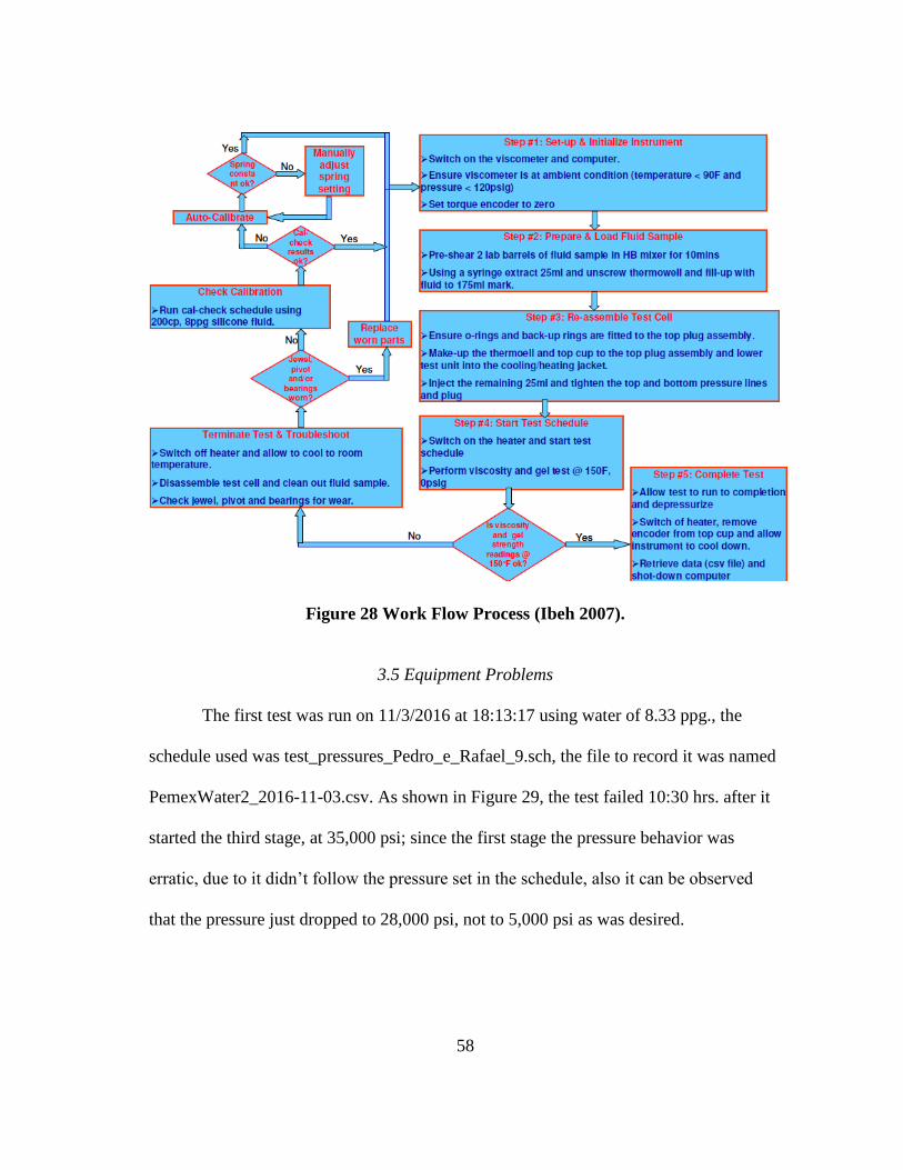
58
Figure 28 Work Flow Process (Ibeh 2007).
3.5 Equipment Problems
The first test was run on 11/3/2016 at 18:13:17 using water of 8.33 ppg., the
schedule used was test_pressures_Pedro_e_Rafael_9.sch, the file to record it was named
PemexWater2_2016-11-03.csv. As shown in Figure 29, the test failed 10:30 hrs. after it
started the third stage, at 35,000 psi; since the first stage the pressure behavior was
erratic, due to it didn’t follow the pressure set in the schedule, also it can be observed
that the pressure just dropped to 28,000 psi, not to 5,000 psi as was desired.
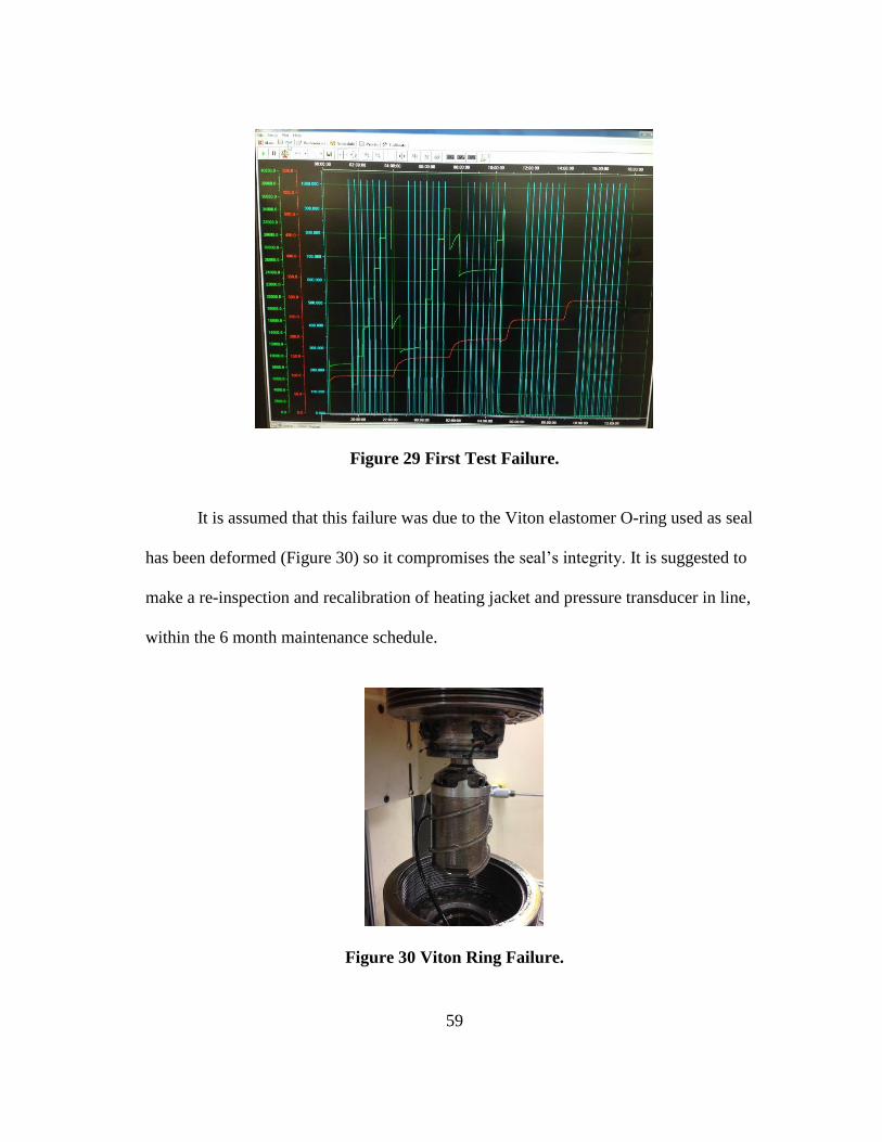
59
Figure 29 First Test Failure.
It is assumed that this failure was due to the Viton elastomer O-ring used as seal
has been deformed (Figure 30) so it compromises the seal’s integrity. It is suggested to
make a re-inspection and recalibration of heating jacket and pressure transducer in line,
within the 6 month maintenance schedule.
Figure 30 Viton Ring Failure.
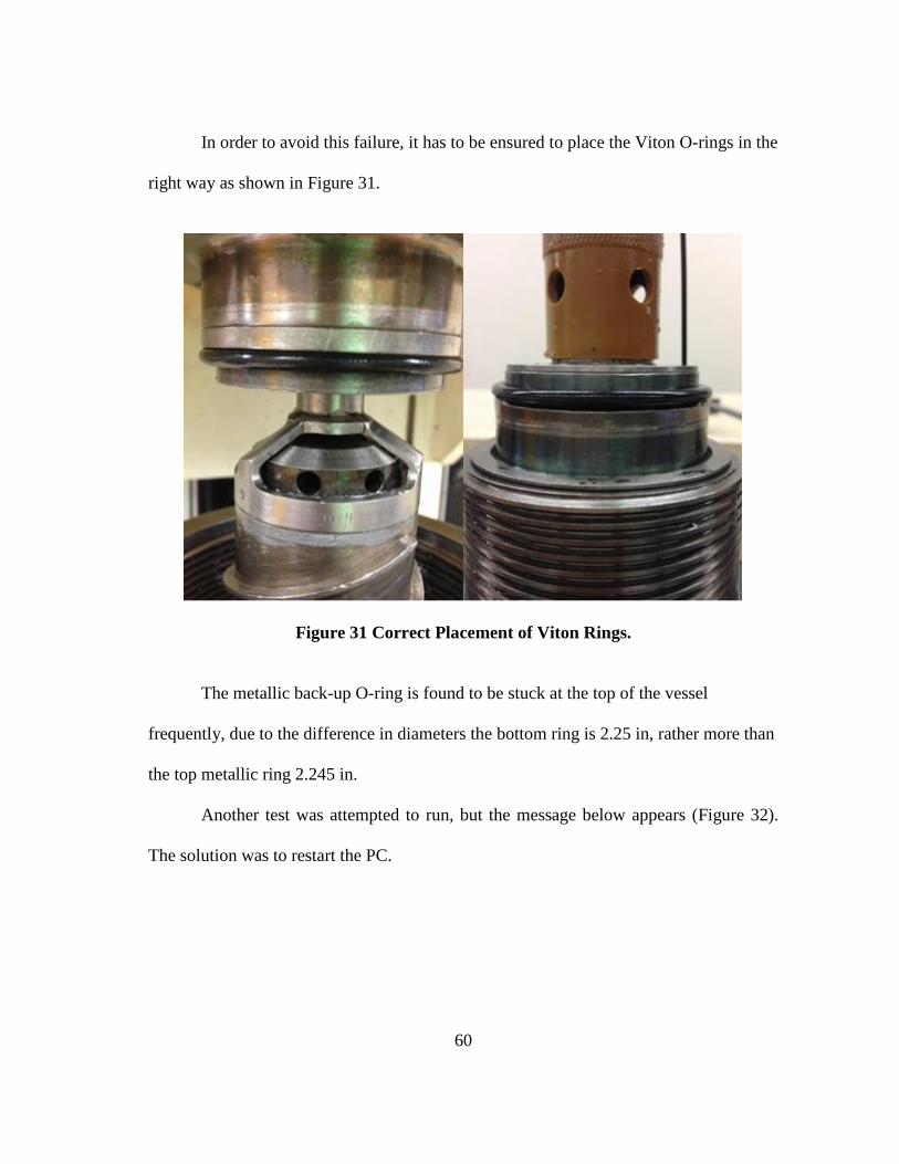
60
In order to avoid this failure, it has to be ensured to place the Viton O-rings in the
right way as shown in Figure 31.
Figure 31 Correct Placement of Viton Rings.
The metallic back-up O-ring is found to be stuck at the top of the vessel
frequently, due to the difference in diameters the bottom ring is 2.25 in, rather more than
the top metallic ring 2.245 in.
Another test was attempted to run, but the message below appears (Figure 32).
The solution was to restart the PC.
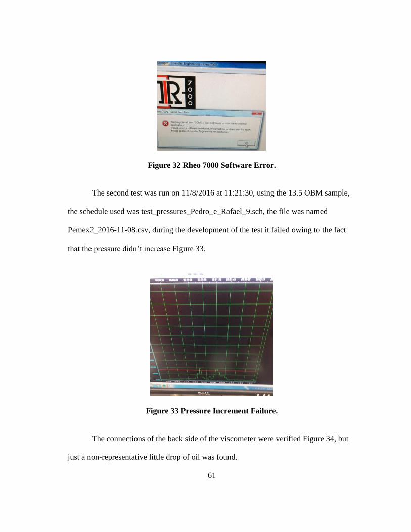
61
Figure 32 Rheo 7000 Software Error.
The second test was run on 11/8/2016 at 11:21:30, using the 13.5 OBM sample,
the schedule used was test_pressures_Pedro_e_Rafael_9.sch, the file was named
Pemex2_2016-11-08.csv, during the development of the test it failed owing to the fact
that the pressure didn’t increase Figure 33.
Figure 33 Pressure Increment Failure.
The connections of the back side of the viscometer were verified Figure 34, but
just a non-representative little drop of oil was found.
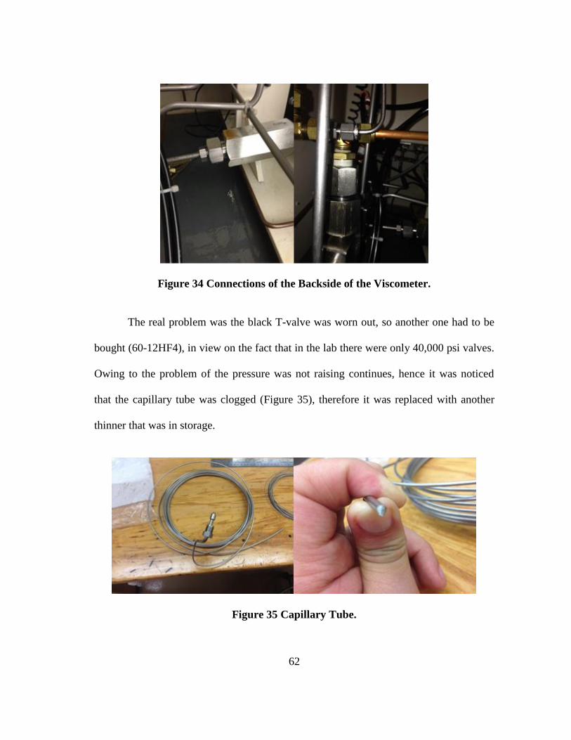
62
Figure 34 Connections of the Backside of the Viscometer.
The real problem was the black T-valve was worn out, so another one had to be
bought (60-12HF4), in view on the fact that in the lab there were only 40,000 psi valves.
Owing to the problem of the pressure was not raising continues, hence it was noticed
that the capillary tube was clogged (Figure 35), therefore it was replaced with another
thinner that was in storage.
Figure 35 Capillary Tube.
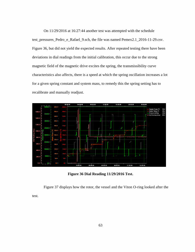
63
On 11/29/2016 at 16:27:44 another test was attempted with the schedule
test_pressures_Pedro_e_Rafael_9.sch, the file was named Pemex2.1_2016-11-29.csv.
Figure 36, but did not yield the expected results. After repeated testing there have been
deviations in dial readings from the initial calibration, this occur due to the strong
magnetic field of the magnetic drive excites the spring, the transmissibility curve
characteristics also affects, there is a speed at which the spring oscillation increases a lot
for a given spring constant and system mass, to remedy this the spring setting has to
recalibrate and manually readjust.
Figure 36 Dial Reading 11/29/2016 Test.
Figure 37 displays how the rotor, the vessel and the Viton O-ring looked after the
test.
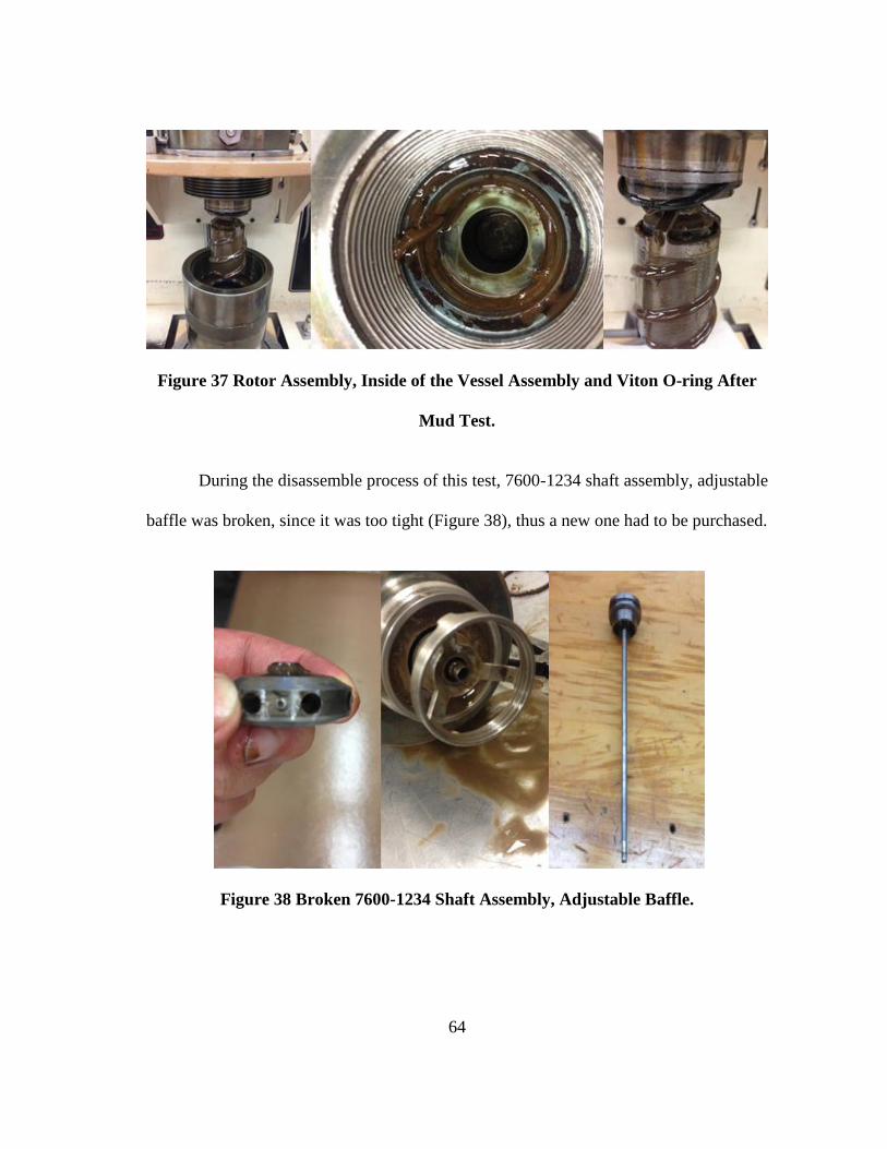
64
Figure 37 Rotor Assembly, Inside of the Vessel Assembly and Viton O-ring After
Mud Test.
During the disassemble process of this test, 7600-1234 shaft assembly, adjustable
baffle was broken, since it was too tight (Figure 38), thus a new one had to be purchased.
Figure 38 Broken 7600-1234 Shaft Assembly, Adjustable Baffle.
65
3.6 Future Improvements
Better Temperature Control: It is necessary to install a cooling system to
control better the temperature. Currently, the cell cools naturally if readings are taken
while cooling down. An ice bucket and a motor can be used as cooling system, because
the original one replacement is so expensive
Rheo 7000 Software: It is needed to solve the skips a step ahead of the desired
step when jumping steps on a pre-designed test schedule in further versions. Besides a
pop-up decision box is needed to save the test data when accidentally the program shuts
down. It must have at least a third rheological model to calculate the properties: the
Herschel-Buckley, as it fits better the performance of drilling fluids, since it has YP and
Power Law does not.
Oil Leakage: There is usually hydraulic oil leaking below the viscometer, after
tests. It is necessary to improve equipment design to contain the oils from the pump
muffler and hoses.
Top plug: It needs another 7600-1181 PIN, VESSEL ALIGNMENT (grip
point), because when the top cap is too tight, it results very difficult to remove it, even
with the strap wrench.
Spring module assembly: The pivot has to be immovable in order to avoid
mistaken dial readings. There must be a spring that allows for higher shear stress
readings.
Timing Belt: It has a lifetime; during the running of one test it was broken,
because it was worn out. It cannot be used any timing belt like one used for cars, due to
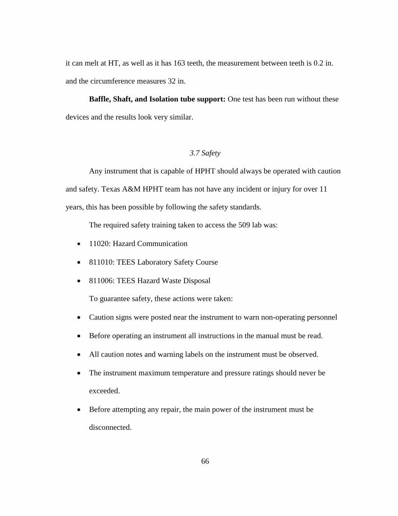
66
it can melt at HT, as well as it has 163 teeth, the measurement between teeth is 0.2 in.
and the circumference measures 32 in.
Baffle, Shaft, and Isolation tube support: One test has been run without these
devices and the results look very similar.
3.7 Safety
Any instrument that is capable of HPHT should always be operated with caution
and safety. Texas A&M HPHT team has not have any incident or injury for over 11
years, this has been possible by following the safety standards.
The required safety training taken to access the 509 lab was:
11020: Hazard Communication
811010: TEES Laboratory Safety Course
811006: TEES Hazard Waste Disposal
To guarantee safety, these actions were taken:
Caution signs were posted near the instrument to warn non-operating personnel
Before operating an instrument all instructions in the manual must be read.
All caution notes and warning labels on the instrument must be observed.
The instrument maximum temperature and pressure ratings should never be
exceeded.
Before attempting any repair, the main power of the instrument must be
disconnected.
67
The heater, power switch, air compressor at the end of each test must be turned
OFF.
Fire extinguishers within close proximity to the instrument are necessary to be
located.
The oil on the heated surfaces that may pose a hazard to starting a test must be
removed.
Open the pressure vessel until temperature is below 100 ºF.
It is necessary to inspect the cell prior to any test.
When working with drilling fluids and heavy lifting equipment the following
personal protective equipment (PPE) is needed:
Organic vapor respirator
Chemical resistant clothing with a protective apron
Nitrile hand gloves
Splash goggles
Rubber-soled safety boots.
All waste fluids and materials are safely contained and appropriately disposed
The Material Safety Data Sheet (MSDS) of every material was obtained and read prior
to storage or use.
In 81010 are contained all emergency exit and first aid procedures. If a spill
happens, these are the steps to follow:
While wearing PPE locate the source of spill and stop.
Absorb the spilled hydraulic oil and dispose in according to 811006.

68
Clean the floor with a scrub and allow drying to avoid slipping.
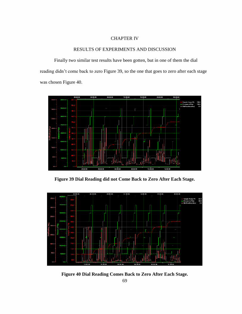
69
CHAPTER IV
RESULTS OF EXPERIMENTS AND DISCUSSION
Finally two similar test results have been gotten, but in one of them the dial
reading didn’t come back to zero Figure 39, so the one that goes to zero after each stage
was chosen Figure 40.
Figure 39 Dial Reading did not Come Back to Zero After Each Stage.
Figure 40 Dial Reading Comes Back to Zero After Each Stage.
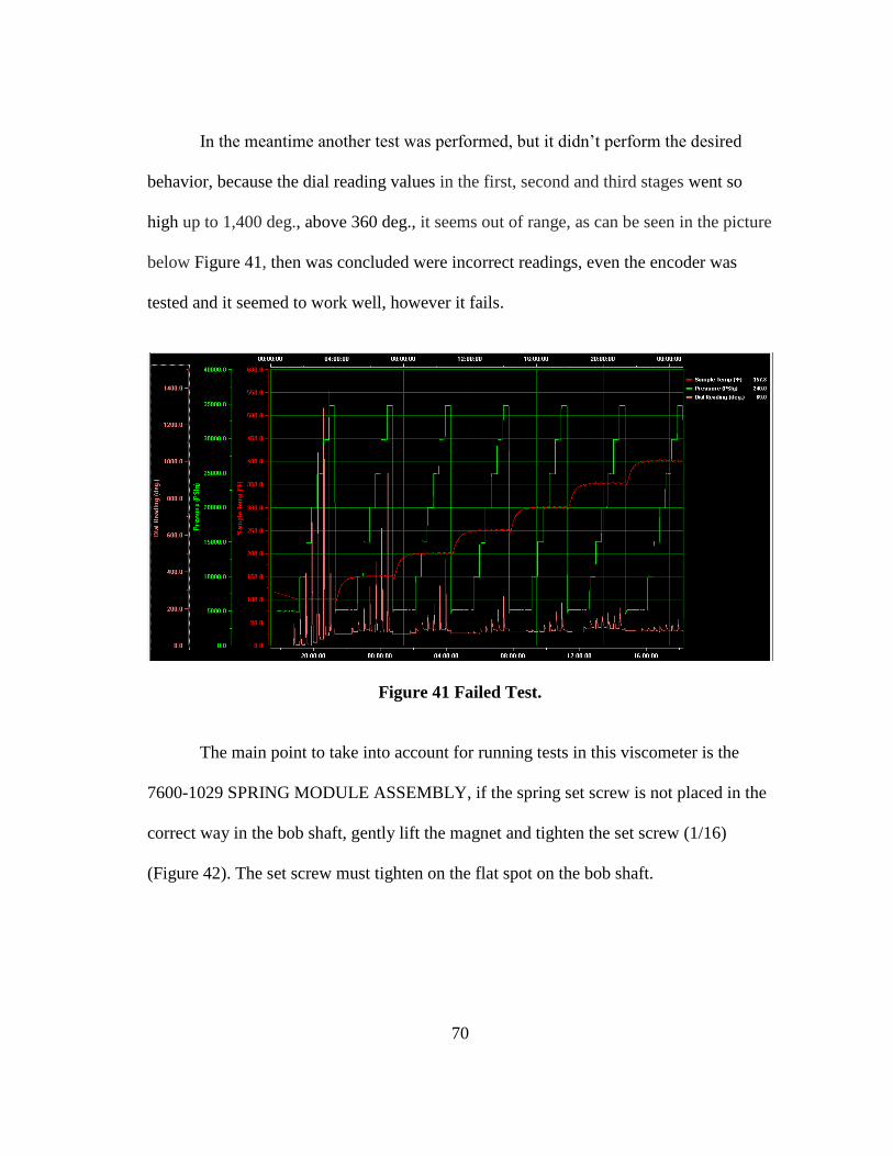
70
In the meantime another test was performed, but it didn’t perform the desired
behavior, because the dial reading values in the first, second and third stages went so
high up to 1,400 deg., above 360 deg., it seems out of range, as can be seen in the picture
below Figure 41, then was concluded were incorrect readings, even the encoder was
tested and it seemed to work well, however it fails.
Figure 41 Failed Test.
The main point to take into account for running tests in this viscometer is the
7600-1029 SPRING MODULE ASSEMBLY, if the spring set screw is not placed in the
correct way in the bob shaft, gently lift the magnet and tighten the set screw (1/16)
(Figure 42). The set screw must tighten on the flat spot on the bob shaft.
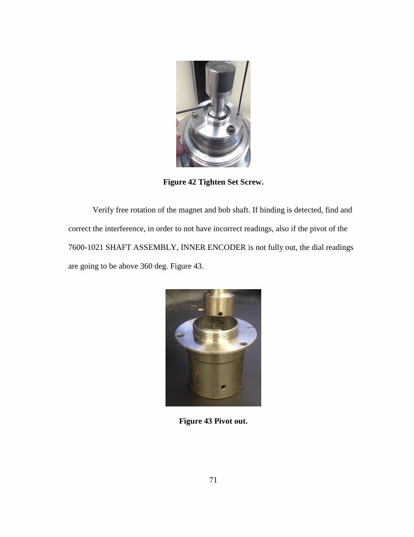
71
Figure 42 Tighten Set Screw.
Verify free rotation of the magnet and bob shaft. If binding is detected, find and
correct the interference, in order to not have incorrect readings, also if the pivot of the
7600-1021 SHAFT ASSEMBLY, INNER ENCODER is not fully out, the dial readings
are going to be above 360 deg. Figure 43.
Figure 43 Pivot out.
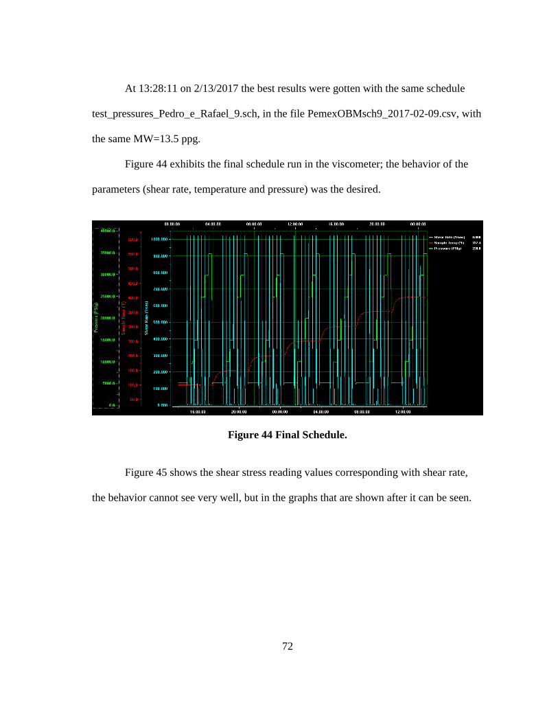
72
At 13:28:11 on 2/13/2017 the best results were gotten with the same schedule
test_pressures_Pedro_e_Rafael_9.sch, in the file PemexOBMsch9_2017-02-09.csv, with
the same MW=13.5 ppg.
Figure 44 exhibits the final schedule run in the viscometer; the behavior of the
parameters (shear rate, temperature and pressure) was the desired.
Figure 44 Final Schedule.
Figure 45 shows the shear stress reading values corresponding with shear rate,
the behavior cannot see very well, but in the graphs that are shown after it can be seen.
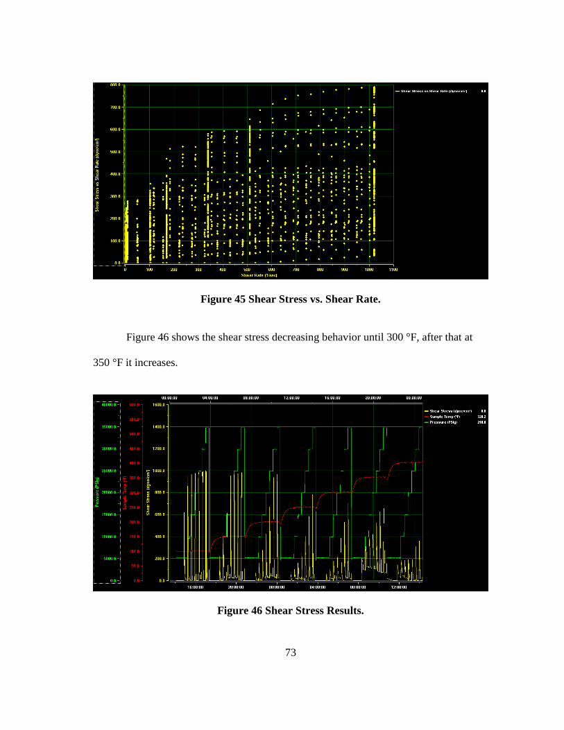
73
Figure 45 Shear Stress vs. Shear Rate.
Figure 46 shows the shear stress decreasing behavior until 300 °F, after that at
350 °F it increases.
Figure 46 Shear Stress Results.
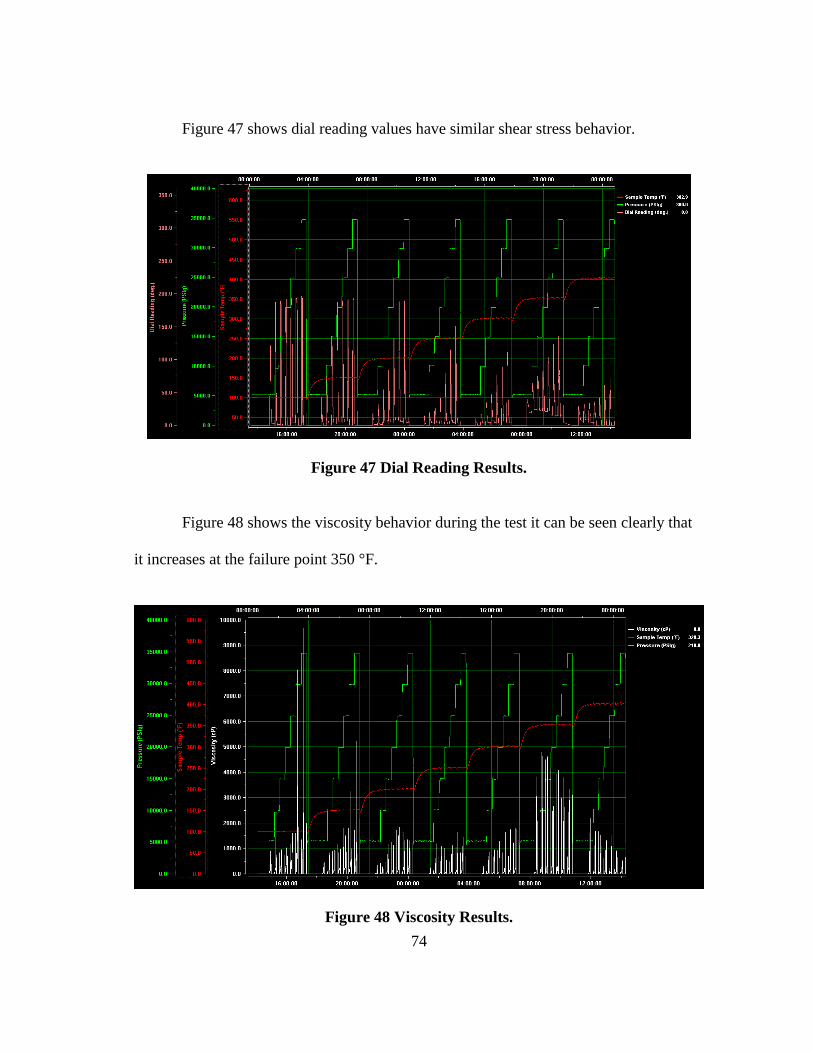
74
Figure 47 shows dial reading values have similar shear stress behavior.
Figure 47 Dial Reading Results.
Figure 48 shows the viscosity behavior during the test it can be seen clearly that
it increases at the failure point 350 °F.
Figure 48 Viscosity Results.
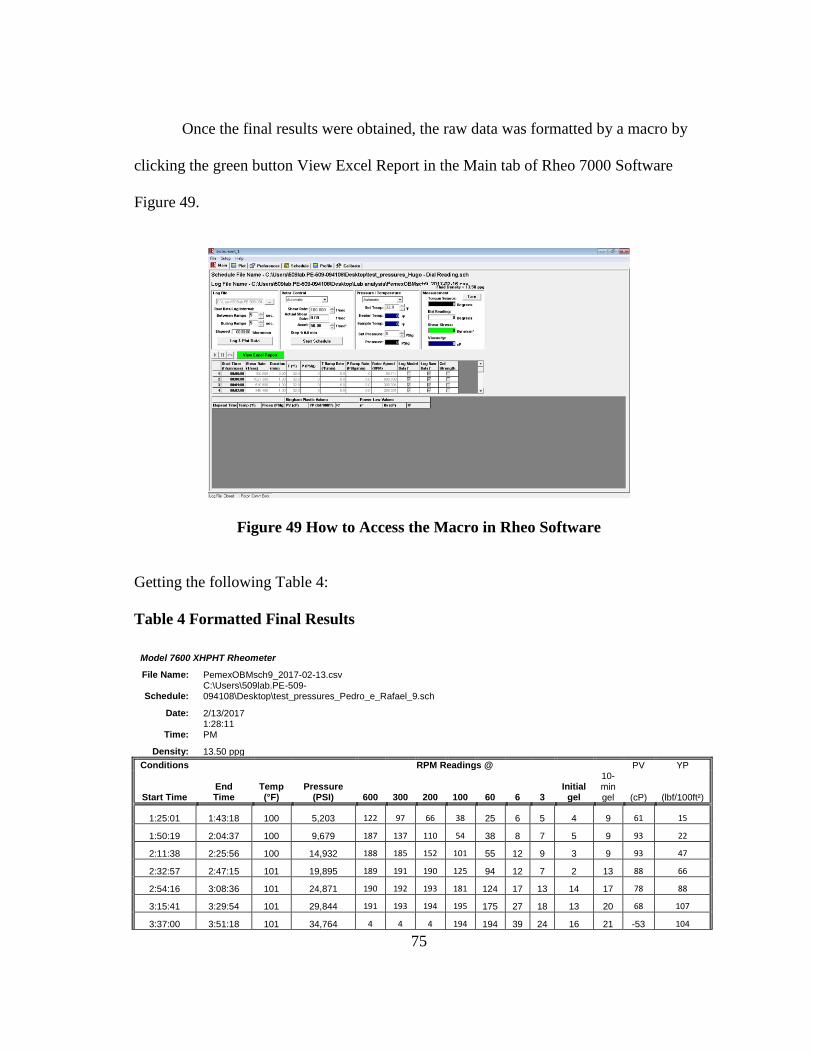
75
Once the final results were obtained, the raw data was formatted by a macro by
clicking the green button View Excel Report in the Main tab of Rheo 7000 Software
Figure 49.
Figure 49 How to Access the Macro in Rheo Software
Getting the following Table 4:
Table 4 Formatted Final Results
Model 7600 XHPHT Rheometer
File Name: PemexOBMsch9_2017-02-13.csv
Schedule: C:\Users\509lab.PE-509-094108\Desktop\test_pressures_Pedro_e_Rafael_9.sch
Date: 2/13/2017
Time:
1:28:11 PM
Density: 13.50 ppg
Conditions RPM Readings @ PV YP
Start Time End Time
Temp (°F)
Pressure (PSI) 600 300 200 100 60 6 3
Initial gel
10-min gel (cP) (lbf/100ft²)
1:25:01 1:43:18 100 5,203 122 97 66 38 25 6 5 4 9 61 15
1:50:19 2:04:37 100 9,679 187 137 110 54 38 8 7 5 9 93 22
2:11:38 2:25:56 100 14,932 188 185 152 101 55 12 9 3 9 93 47
2:32:57 2:47:15 101 19,895 189 191 190 125 94 12 7 2 13 88 66
2:54:16 3:08:36 101 24,871 190 192 193 181 124 17 13 14 17 78 88
3:15:41 3:29:54 101 29,844 191 193 194 195 175 27 18 13 20 68 107
3:37:00 3:51:18 101 34,764 4 4 4 194 194 39 24 16 21 -53 104
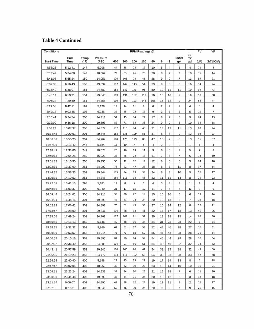
76
Table 4 Continued
Conditions RPM Readings @ PV YP
Start Time End Time
Temp (°F)
Pressure (PSI) 600 300 200 100 60 6 3
Initial gel
10-min gel (cP) (lbf/100ft²)
4:58:23 5:12:41 147 5,208 44 38 28 16 10 5 4 3 4 21 8
5:19:42 5:34:00 149 10,067 73 63 46 25 20 8 7 7 10 35 14
5:41:06 5:55:24 150 14,951 120 105 78 41 28 9 9 7 13 59 21
6:02:30 6:16:43 150 19,894 187 147 113 54 39 9 8 8 16 94 24
6:23:49 6:38:07 151 24,889 188 182 143 93 50 12 11 11 19 94 43
6:45:14 6:59:31 151 29,846 189 191 182 118 76 13 10 7 19 90 60
7:06:32 7:20:50 151 34,758 190 192 193 148 108 16 12 9 24 83 77
8:27:58 8:42:11 197 5,178 19 14 11 8 6 2 2 2 4 8 4
8:49:17 9:03:35 198 9,935 32 25 22 15 9 3 3 3 5 15 7
9:10:41 9:24:54 200 14,911 54 45 34 22 17 8 7 6 9 24 13
9:32:00 9:46:18 200 19,893 82 71 53 33 24 9 9 8 10 38 18
9:53:24 10:07:37 200 24,877 132 110 84 46 31 13 13 11 13 63 24
10:14:43 10:29:01 201 29,846 188 138 109 55 37 8 8 9 12 93 23
10:36:08 10:50:20 201 34,767 188 176 129 83 47 10 9 8 13 95 37
11:57:29 12:11:42 247 5,184 15 10 7 5 4 2 2 2 1 6 3
12:18:49 12:33:06 249 10,073 20 16 13 11 9 6 6 7 5 7 8
12:40:13 12:54:25 250 15,023 32 26 23 16 11 7 6 7 6 13 10
13:01:32 13:15:50 250 19,955 50 42 32 19 12 6 6 6 5 24 10
13:22:56 13:37:09 251 24,902 78 62 47 28 18 8 8 11 8 37 14
13:44:15 13:58:33 251 29,844 115 94 63 38 24 8 8 10 9 56 17
14:05:39 14:19:52 251 34,746 154 116 93 48 33 11 11 14 8 75 22
15:27:01 15:41:13 298 5,181 11 8 7 5 4 3 3 3 1 4 4
15:48:19 16:02:37 300 9,940 21 17 15 12 11 7 7 5 5 7 9
16:09:44 16:24:01 300 14,910 35 30 27 19 15 10 10 6 6 13 14
16:31:04 16:45:16 301 19,890 47 41 34 24 20 13 13 8 7 18 18
16:52:23 17:06:41 301 24,891 76 61 49 33 27 15 14 12 8 32 21
17:13:47 17:28:00 301 29,841 104 88 64 41 32 17 17 13 13 46 26
17:35:06 17:49:24 301 34,762 137 109 91 51 39 18 18 15 14 62 30
18:56:55 19:11:13 350 5,146 40 38 36 34 34 31 28 23 22 5 34
19:18:15 19:32:32 352 9,966 64 61 57 53 52 48 40 28 27 10 51
19:39:39 19:53:57 352 14,914 75 73 68 59 55 47 43 28 28 15 54
20:00:58 20:15:16 353 19,895 82 80 74 59 54 45 44 28 28 20 54
20:22:22 20:36:40 353 24,888 104 97 86 61 54 40 40 32 32 34 52
20:43:41 20:57:59 353 29,846 120 106 96 62 54 38 38 28 32 43 50
21:05:05 21:19:23 353 34,772 133 111 102 66 54 33 33 28 33 52 48
22:26:28 22:40:40 400 5,198 28 25 23 21 19 17 14 13 8 6 18
22:47:47 23:02:05 402 10,059 36 32 30 26 23 18 14 10 10 10 21
23:09:11 23:23:24 402 14,932 37 34 30 26 21 16 15 7 6 11 20
23:30:30 23:44:48 402 19,893 37 34 31 24 20 13 12 8 3 12 18
23:51:54 0:06:07 402 24,890 42 38 32 24 19 11 11 9 2 16 17
0:13:13 0:27:31 402 29,846 60 46 39 24 20 9 9 7 9 26 15
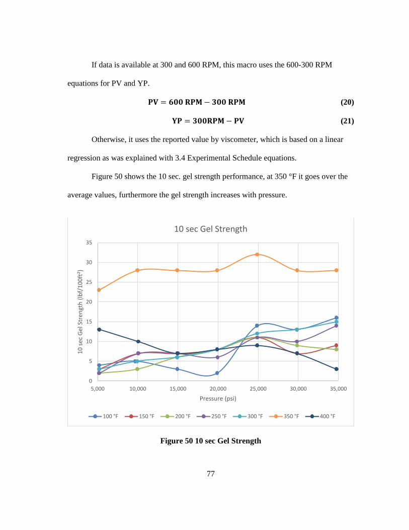
77
If data is available at 300 and 600 RPM, this macro uses the 600-300 RPM
equations for PV and YP.
(20)
(21)
Otherwise, it uses the reported value by viscometer, which is based on a linear
regression as was explained with 3.4 Experimental Schedule equations.
Figure 50 shows the 10 sec. gel strength performance, at 350 °F it goes over the
average values, furthermore the gel strength increases with pressure.
Figure 50 10 sec Gel Strength
0
5
10
15
20
25
30
35
5,000 10,000 15,000 20,000 25,000 30,000 35,000
10
sec
Gel
Str
engt
h (
lbf/
10
0ft
²)
Pressure (psi)
10 sec Gel Strength
100 °F 150 °F 200 °F 250 °F 300 °F 350 °F 400 °F
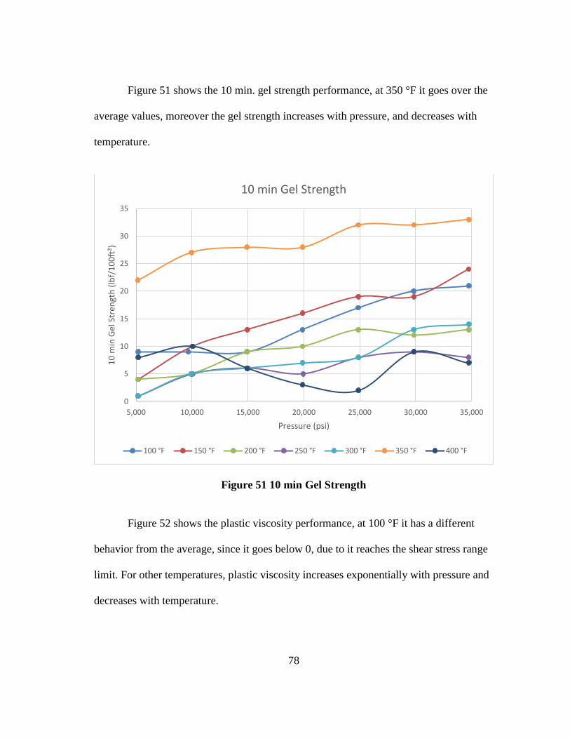
78
Figure 51 shows the 10 min. gel strength performance, at 350 °F it goes over the
average values, moreover the gel strength increases with pressure, and decreases with
temperature.
Figure 51 10 min Gel Strength
Figure 52 shows the plastic viscosity performance, at 100 °F it has a different
behavior from the average, since it goes below 0, due to it reaches the shear stress range
limit. For other temperatures, plastic viscosity increases exponentially with pressure and
decreases with temperature.
0
5
10
15
20
25
30
35
5,000 10,000 15,000 20,000 25,000 30,000 35,000
10
min
Gel
Str
engt
h (
lbf/
10
0ft
²)
Pressure (psi)
10 min Gel Strength
100 °F 150 °F 200 °F 250 °F 300 °F 350 °F 400 °F
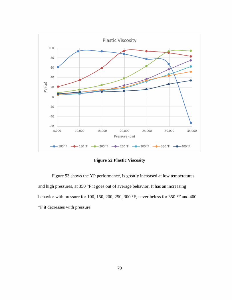
79
Figure 52 Plastic Viscosity
Figure 53 shows the YP performance, is greatly increased at low temperatures
and high pressures, at 350 °F it goes out of average behavior. It has an increasing
behavior with pressure for 100, 150, 200, 250, 300 °F, nevertheless for 350 °F and 400
°F it decreases with pressure.
-60
-40
-20
0
20
40
60
80
100
5,000 10,000 15,000 20,000 25,000 30,000 35,000
PV
(cp
)
Pressure (psi)
Plastic Viscosity
100 °F 150 °F 200 °F 250 °F 300 °F 350 °F 400 °F
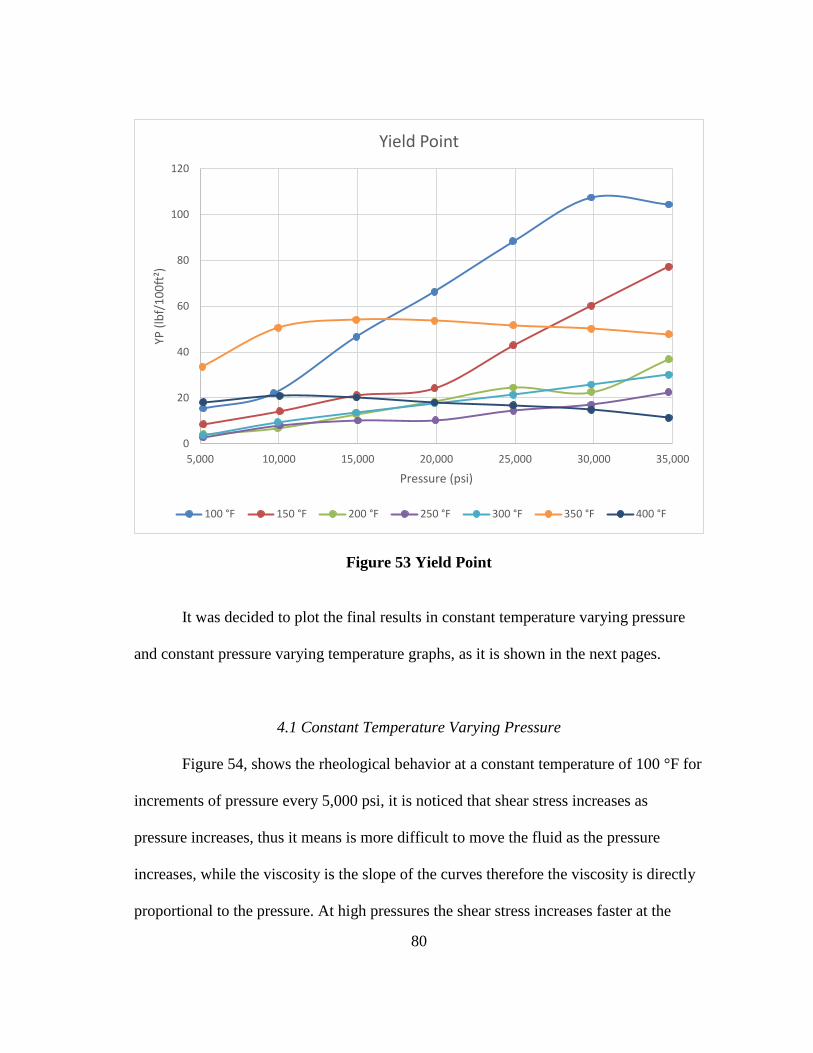
80
Figure 53 Yield Point
It was decided to plot the final results in constant temperature varying pressure
and constant pressure varying temperature graphs, as it is shown in the next pages.
4.1 Constant Temperature Varying Pressure
Figure 54, shows the rheological behavior at a constant temperature of 100 °F for
increments of pressure every 5,000 psi, it is noticed that shear stress increases as
pressure increases, thus it means is more difficult to move the fluid as the pressure
increases, while the viscosity is the slope of the curves therefore the viscosity is directly
proportional to the pressure. At high pressures the shear stress increases faster at the
0
20
40
60
80
100
120
5,000 10,000 15,000 20,000 25,000 30,000 35,000
YP (
lbf/
10
0ft
²)
Pressure (psi)
Yield Point
100 °F 150 °F 200 °F 250 °F 300 °F 350 °F 400 °F
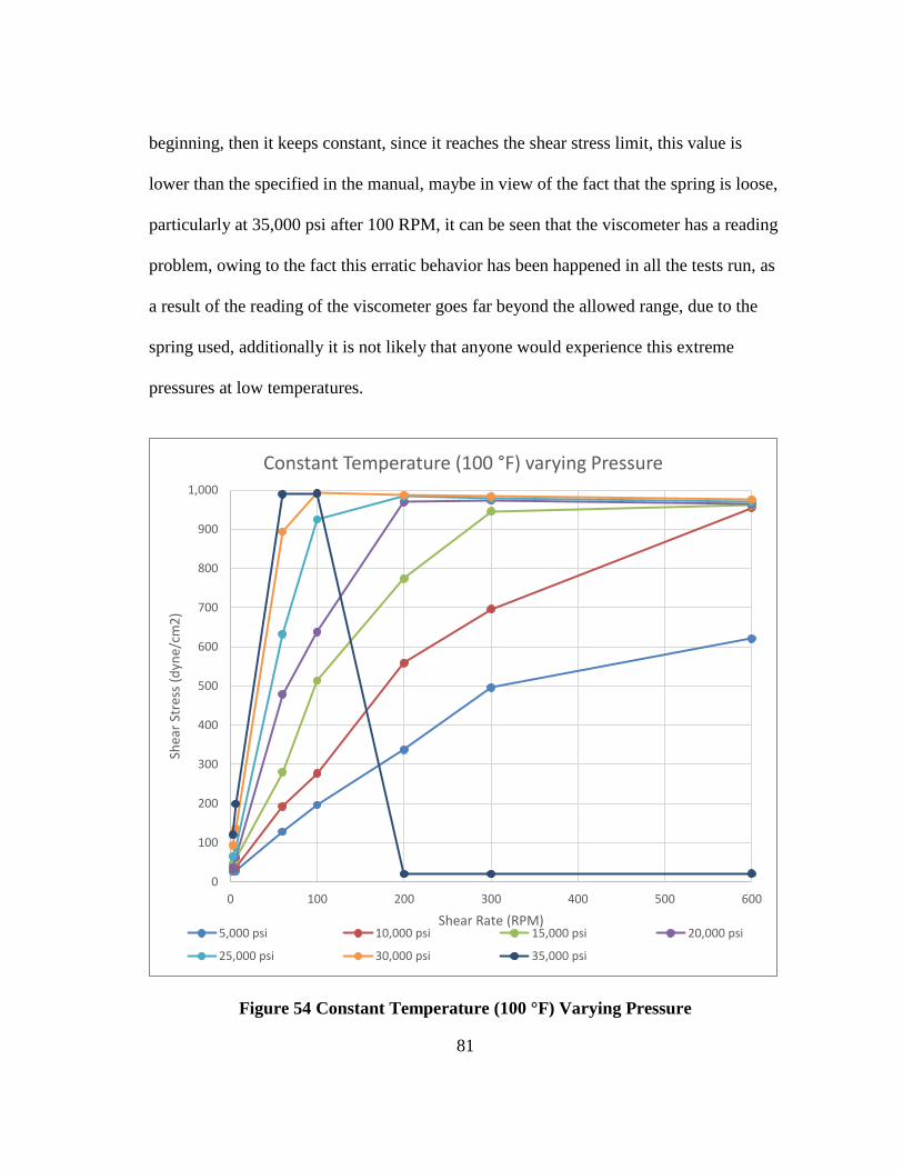
81
beginning, then it keeps constant, since it reaches the shear stress limit, this value is
lower than the specified in the manual, maybe in view of the fact that the spring is loose,
particularly at 35,000 psi after 100 RPM, it can be seen that the viscometer has a reading
problem, owing to the fact this erratic behavior has been happened in all the tests run, as
a result of the reading of the viscometer goes far beyond the allowed range, due to the
spring used, additionally it is not likely that anyone would experience this extreme
pressures at low temperatures.
Figure 54 Constant Temperature (100 °F) Varying Pressure
0
100
200
300
400
500
600
700
800
900
1,000
0 100 200 300 400 500 600
Shea
r St
ress
(d
yne/
cm2
)
Shear Rate (RPM)
Constant Temperature (100 °F) varying Pressure
5,000 psi 10,000 psi 15,000 psi 20,000 psi
25,000 psi 30,000 psi 35,000 psi
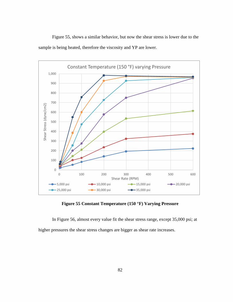
82
Figure 55, shows a similar behavior, but now the shear stress is lower due to the
sample is being heated, therefore the viscosity and YP are lower.
Figure 55 Constant Temperature (150 °F) Varying Pressure
In Figure 56, almost every value fit the shear stress range, except 35,000 psi; at
higher pressures the shear stress changes are bigger as shear rate increases.
0
100
200
300
400
500
600
700
800
900
1,000
0 100 200 300 400 500 600
Shea
r St
ress
(d
yne/
cm2
)
Shear Rate (RPM)
Constant Temperature (150 °F) varying Pressure
5,000 psi 10,000 psi 15,000 psi 20,000 psi
25,000 psi 30,000 psi 35,000 psi
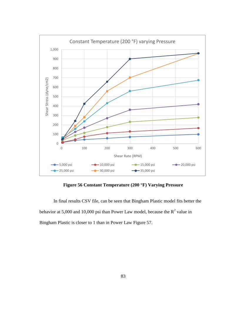
83
Figure 56 Constant Temperature (200 °F) Varying Pressure
In final results CSV file, can be seen that Bingham Plastic model fits better the
behavior at 5,000 and 10,000 psi than Power Law model, because the R2 value in
Bingham Plastic is closer to 1 than in Power Law Figure 57.
0
100
200
300
400
500
600
700
800
900
1,000
0 100 200 300 400 500 600
Shea
r St
ress
(d
yne/
cm2
)
Shear Rate (RPM)
Constant Temperature (200 °F) varying Pressure
5,000 psi 10,000 psi 15,000 psi 20,000 psi
25,000 psi 30,000 psi 35,000 psi
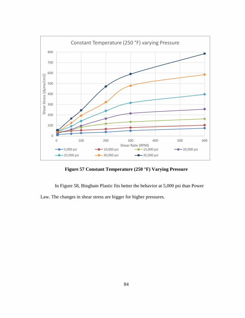
84
Figure 57 Constant Temperature (250 °F) Varying Pressure
In Figure 58, Bingham Plastic fits better the behavior at 5,000 psi than Power
Law. The changes in shear stress are bigger for higher pressures.
0
100
200
300
400
500
600
700
800
0 100 200 300 400 500 600
Shea
r St
ress
(d
yme/
cm2
)
Shear Rate (RPM)
Constant Temperature (250 °F) varying Pressure
5,000 psi 10,000 psi 15,000 psi 20,000 psi
25,000 psi 30,000 psi 35,000 psi
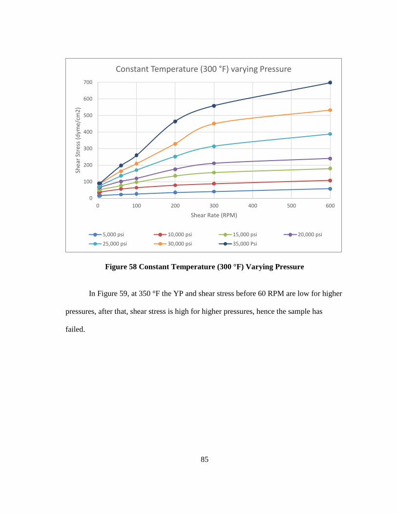
85
Figure 58 Constant Temperature (300 °F) Varying Pressure
In Figure 59, at 350 °F the YP and shear stress before 60 RPM are low for higher
pressures, after that, shear stress is high for higher pressures, hence the sample has
failed.
0
100
200
300
400
500
600
700
0 100 200 300 400 500 600
Shea
r St
ress
(d
yme/
cm2
)
Shear Rate (RPM)
Constant Temperature (300 °F) varying Pressure
5,000 psi 10,000 psi 15,000 psi 20,000 psi
25,000 psi 30,000 psi 35,000 Psi
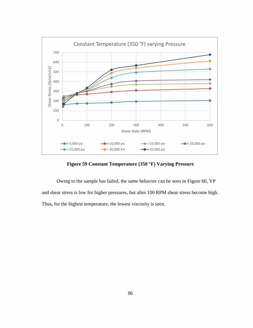
86
Figure 59 Constant Temperature (350 °F) Varying Pressure
Owing to the sample has failed, the same behavior can be seen in Figure 60, YP
and shear stress is low for higher pressures, but after 100 RPM shear stress become high.
Thus, for the highest temperature, the lowest viscosity is seen.
0
100
200
300
400
500
600
700
0 100 200 300 400 500 600
Shea
r St
ress
(d
yne/
cm2
)
Shear Rate (RPM)
Constant Temperature (350 °F) varying Pressure
5,000 psi 10,000 psi 15,000 psi 20,000 psi
25,000 psi 30,000 Psi 35,000 psi
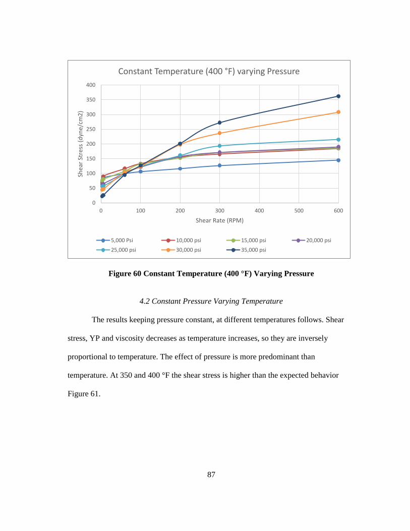
87
Figure 60 Constant Temperature (400 °F) Varying Pressure
4.2 Constant Pressure Varying Temperature
The results keeping pressure constant, at different temperatures follows. Shear
stress, YP and viscosity decreases as temperature increases, so they are inversely
proportional to temperature. The effect of pressure is more predominant than
temperature. At 350 and 400 °F the shear stress is higher than the expected behavior
Figure 61.
0
50
100
150
200
250
300
350
400
0 100 200 300 400 500 600
Shea
r St
ress
(d
yne/
cm2
)
Shear Rate (RPM)
Constant Temperature (400 °F) varying Pressure
5,000 Psi 10,000 psi 15,000 psi 20,000 psi
25,000 psi 30,000 psi 35,000 psi
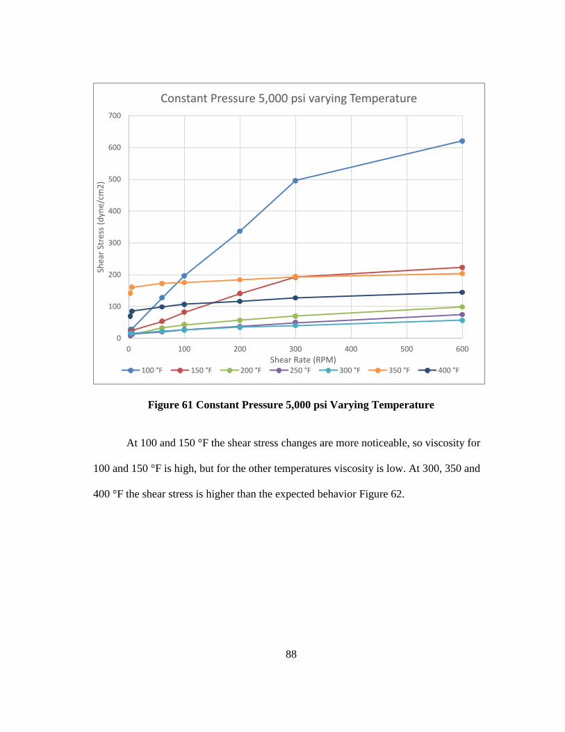
88
Figure 61 Constant Pressure 5,000 psi Varying Temperature
At 100 and 150 °F the shear stress changes are more noticeable, so viscosity for
100 and 150 °F is high, but for the other temperatures viscosity is low. At 300, 350 and
400 °F the shear stress is higher than the expected behavior Figure 62.
0
100
200
300
400
500
600
700
0 100 200 300 400 500 600
Shea
r St
ress
(d
yne/
cm2
)
Shear Rate (RPM)
Constant Pressure 5,000 psi varying Temperature
100 °F 150 °F 200 °F 250 °F 300 °F 350 °F 400 °F
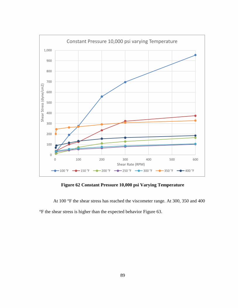
89
Figure 62 Constant Pressure 10,000 psi Varying Temperature
At 100 °F the shear stress has reached the viscometer range. At 300, 350 and 400
°F the shear stress is higher than the expected behavior Figure 63.
0
100
200
300
400
500
600
700
800
900
1,000
0 100 200 300 400 500 600
Shea
r St
ress
(d
yne/
cm2
)
Shear Rate (RPM)
Constant Pressure 10,000 psi varying Temperature
100 °F 150 °F 200 °F 250 °F 300 °F 350 °F 400 °F
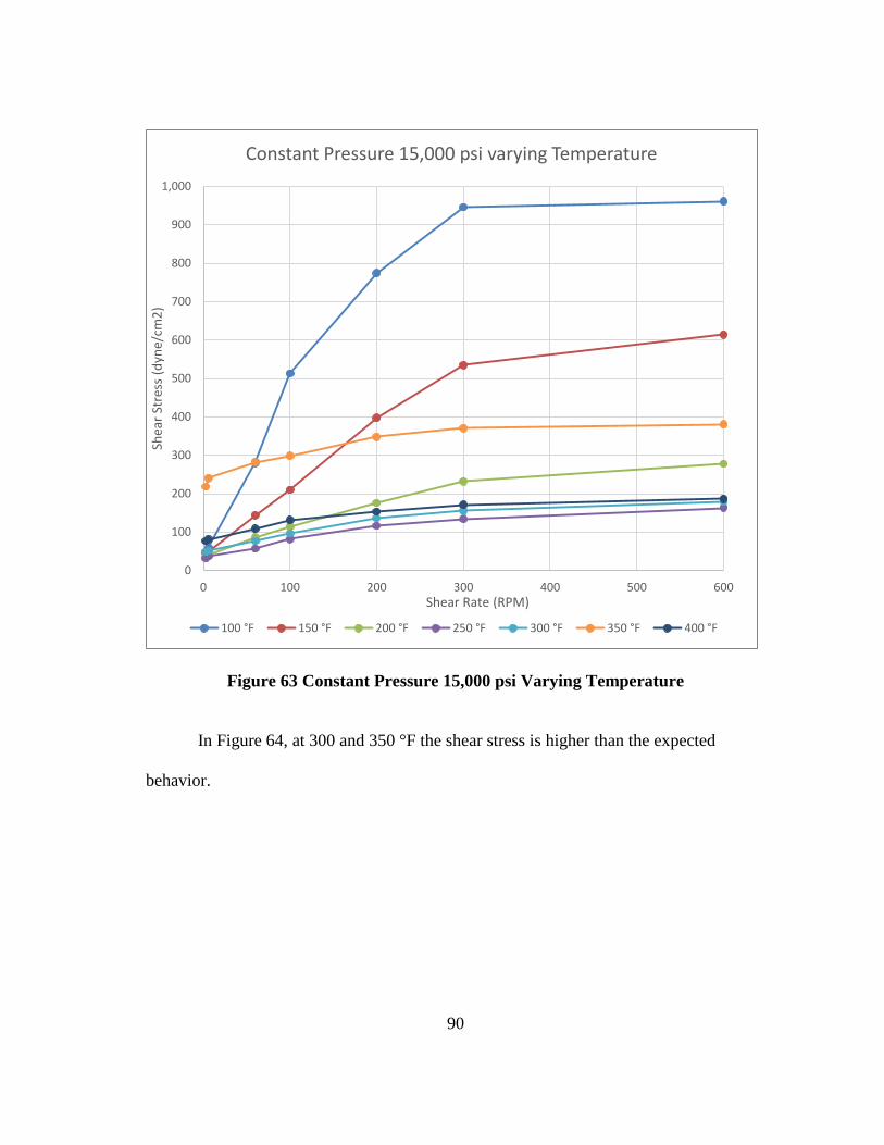
90
Figure 63 Constant Pressure 15,000 psi Varying Temperature
In Figure 64, at 300 and 350 °F the shear stress is higher than the expected
behavior.
0
100
200
300
400
500
600
700
800
900
1,000
0 100 200 300 400 500 600
Shea
r St
ress
(d
yne/
cm2
)
Shear Rate (RPM)
Constant Pressure 15,000 psi varying Temperature
100 °F 150 °F 200 °F 250 °F 300 °F 350 °F 400 °F
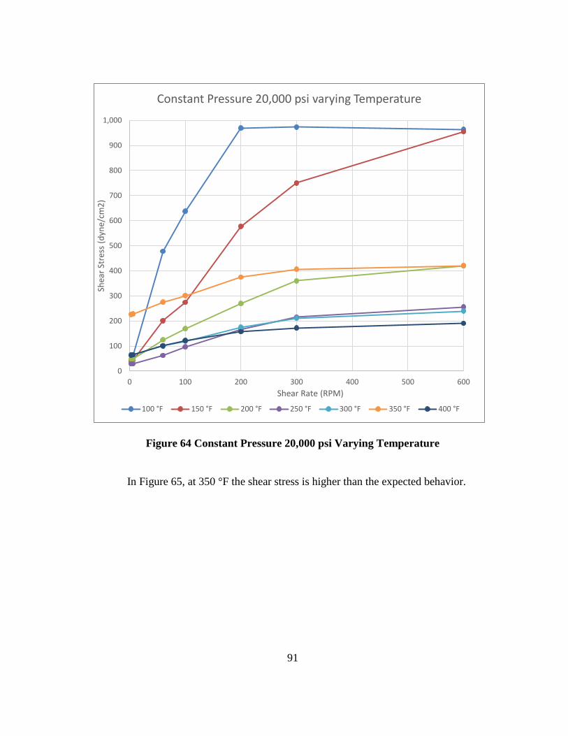
91
Figure 64 Constant Pressure 20,000 psi Varying Temperature
In Figure 65, at 350 °F the shear stress is higher than the expected behavior.
0
100
200
300
400
500
600
700
800
900
1,000
0 100 200 300 400 500 600
Shea
r St
ress
(d
yne/
cm2
)
Shear Rate (RPM)
Constant Pressure 20,000 psi varying Temperature
100 °F 150 °F 200 °F 250 °F 300 °F 350 °F 400 °F
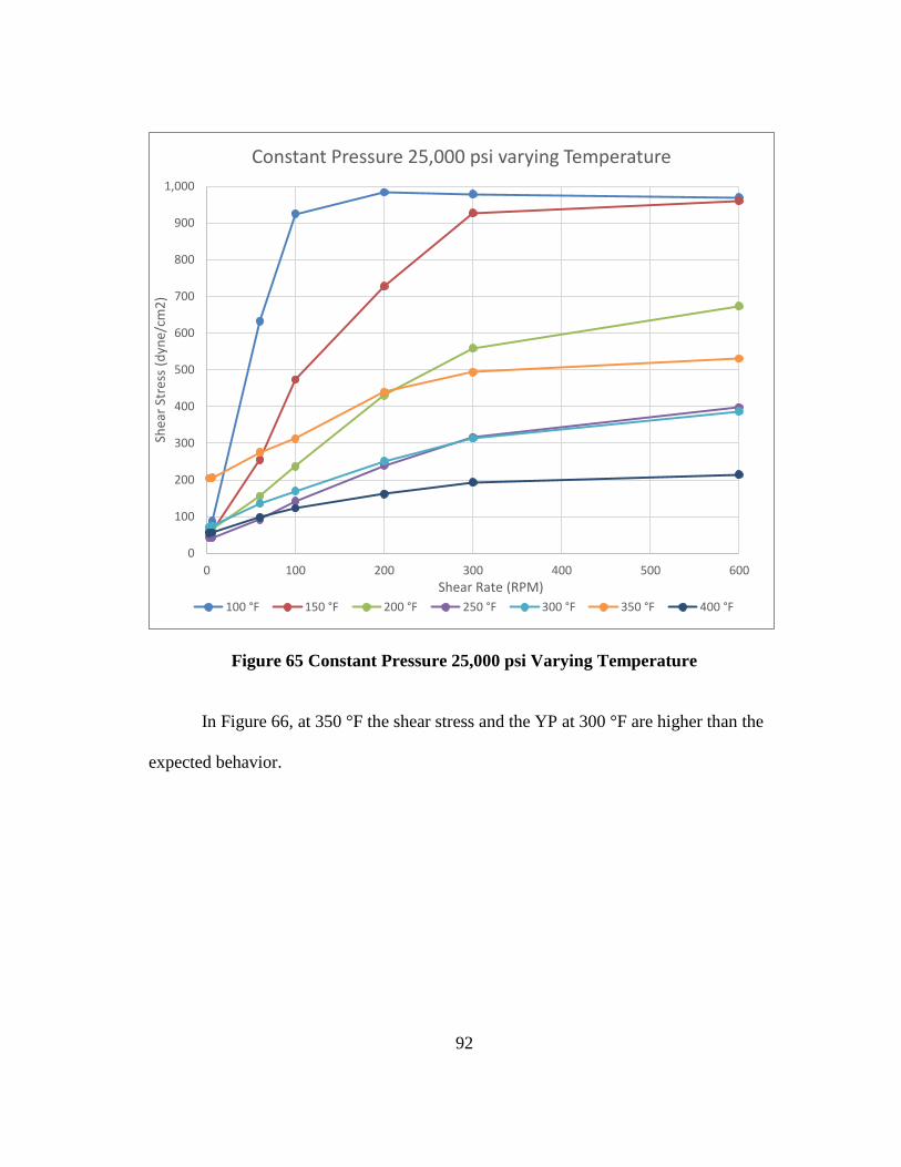
92
Figure 65 Constant Pressure 25,000 psi Varying Temperature
In Figure 66, at 350 °F the shear stress and the YP at 300 °F are higher than the
expected behavior.
0
100
200
300
400
500
600
700
800
900
1,000
0 100 200 300 400 500 600
Shea
r St
ress
(d
yne/
cm2
)
Shear Rate (RPM)
Constant Pressure 25,000 psi varying Temperature
100 °F 150 °F 200 °F 250 °F 300 °F 350 °F 400 °F
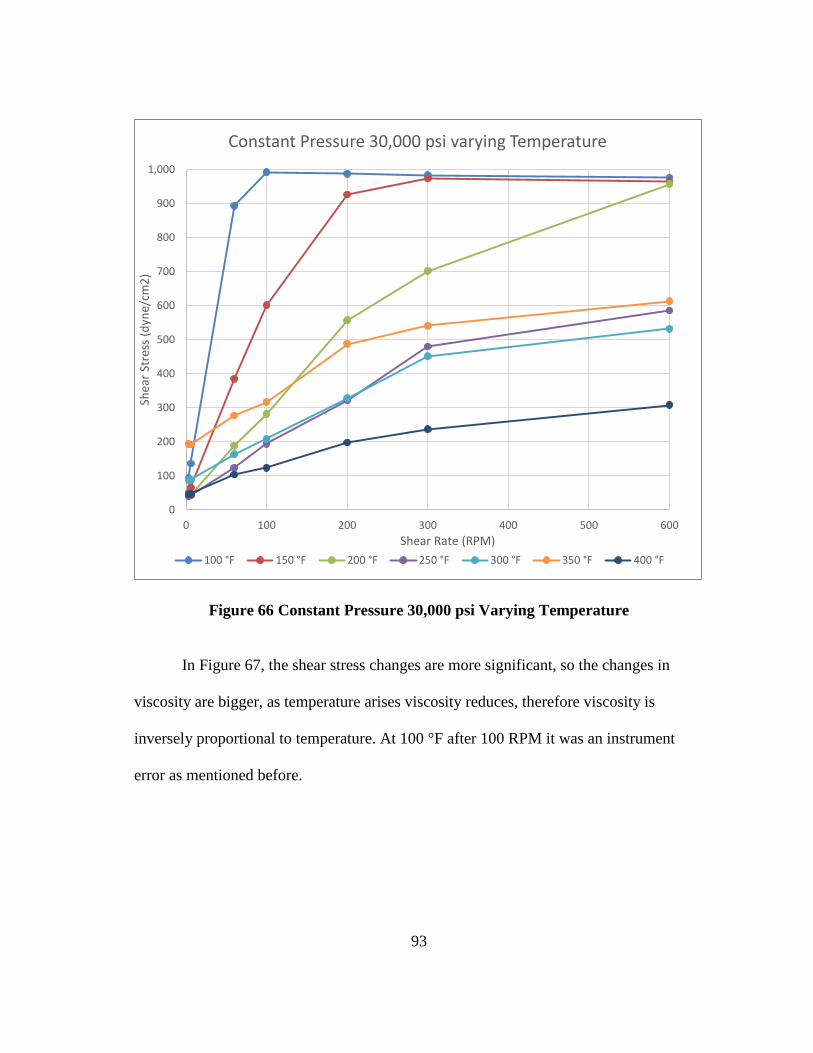
93
Figure 66 Constant Pressure 30,000 psi Varying Temperature
In Figure 67, the shear stress changes are more significant, so the changes in
viscosity are bigger, as temperature arises viscosity reduces, therefore viscosity is
inversely proportional to temperature. At 100 °F after 100 RPM it was an instrument
error as mentioned before.
0
100
200
300
400
500
600
700
800
900
1,000
0 100 200 300 400 500 600
Shea
r St
ress
(d
yne/
cm2
)
Shear Rate (RPM)
Constant Pressure 30,000 psi varying Temperature
100 °F 150 °F 200 °F 250 °F 300 °F 350 °F 400 °F
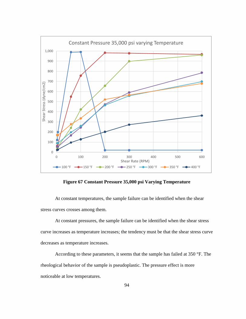
94
Figure 67 Constant Pressure 35,000 psi Varying Temperature
At constant temperatures, the sample failure can be identified when the shear
stress curves crosses among them.
At constant pressures, the sample failure can be identified when the shear stress
curve increases as temperature increases; the tendency must be that the shear stress curve
decreases as temperature increases.
According to these parameters, it seems that the sample has failed at 350 °F. The
rheological behavior of the sample is pseudoplastic. The pressure effect is more
noticeable at low temperatures.
0
100
200
300
400
500
600
700
800
900
1,000
0 100 200 300 400 500 600
Shea
r St
ress
(d
yne/
cm2
)
Shear Rate (RPM)
Constant Pressure 35,000 psi varying Temperature
100 °F 150 °F 200 °F 250 °F 300 °F 350 °F 400 °F

95
The water test was run, yet a Newtonian behavior was just performed at 5,000,
10,000 and 15,000 psi, above these pressures an anomalous behavior was performed,
due to as more DURATHERM oil is needed to achieve the pressure, it mixes with the
sample.
96
CHAPTER V
CONCLUSIONS, RECOMMENDATIONS AND FUTURE WORK
Throughout the performance of these tests, it is necessary to pay close attention
to the spring module assembly, as it is the part that gave the dial reading lectures and
hence the shear stress lectures and it is very sensitive to a loose spring and if the pivot is
not placed correctly the lectures will be very high, also the screw has to be set in the flat
part of the shaft of the bob.
The rheogram´s curves fit 2nd
polynomial functions very well, especially at
constant temperature. The R-squared values are all between 0.95 and 0.99, until the
temperature hits 300 °F.
In summary, it is necessary to continue studying the rheological properties of the
drilling fluids at xHPHT conditions (300 to 600 °F and 20,000 to 40,000 psi), because
there is little information. The main focus of this research is to study the rheological
behavior of an OBM sample at these extreme conditions. In future research work, it
would be interesting to evaluate the performance of other fluids, for example by getting
a formate brine sample.
Currently another research is being done for adapting the viscometer to simulate
gas influx in order to avoid the mixture problem, by constructing an extreme HPHT PVT
cell to have the ability to measure properties of drilling fluids, reservoir gasses, and its
solubility in drilling fluids for conditions equivalent to the Model 7600 HPHT
Viscometer. The goal is then to inject the gas laden drilling fluid into the Model 7600

97
HPHT Viscometer to determine the effect of the gas on the rheological properties of
drilling fluids. This will allow developing an xHPHT gas kick behavior simulator.
98
REFERENCES
Abduo, M. I., A. S. Dahab, H. Abuseda et al. 2015. Comparative study of using Water-
Based mud containing Multiwall Carbon Nanotubes versus Oil-Based mud in
HPHT fields. Egyptian Journal of Petroleum.
Adamson, K., G. Birch, E. Gao et al. 1998. High-Pressure, High-Temperature Well
Construction. Oilfield Review. Pag. 36-49.
Amani, M. 2012. The Rheological Properties of Oil-Based Mud Under High Pressure
and High Temperature Conditions. Advances in Petroleum Exploration and
Development. Vol. 3. Iss. 2. Pag. 21-30.
Amani, M., M Al-Jubouri, A. Shadravan. 2012. Comparative Study of Using Oil-Based
Mud Versus Water-Based Mud in HPHT Fields. Advances in Petroleum
Exploration and Development. Vol. 4. Iss. 2. Pag. 18-27.
Amani, M., M. Al-Jubouri. 2012. The Effect of High Pressures and High Temperatures
on the Properties of Water Based Drilling Fluids. Energy Science and
Technology. Vol. 4. Iss. 1. Pag. 27-33.
Amani, M., A. Retnanto, R. Yrac et al. 2015. Effect of salinity on the viscosity of water
based drilling fluids at elevated pressures and temperatures. International
Journal of Engineering and Applied Sciences. Vol. 7. Iss. 4. Pag. 30-52.
Anoop, K., R. Sadr, M. Al-Jubouri et al. 2014. Rheology of mineral oil-SiO2 nanofluids
at high pressure and high temperatures. International Journal of Thermal
Sciences. Vol. 77. Pag. 108-115.
99
Bland, R. G., G. A. Mullen, Y. N. Gonzalez et al. 2006. HPHT Drilling Fluid
Challenges. IADC/SPE Asia Pacific Drilling Technology Conference and
Exhibition, Bangkok, Thailand, SPE-103731-MS.
Bourgoyne, A. T., Jr., K. K. Millheim, M. E. Chenevert et al. 1986. Applied Drilling
Engineering, Society of Petroleum Engineers (Reprint). SPE-31656-MS
De Stefano, G., E. Stamatakis, S. Young. 2012. Meeting the Ultrahigh-
Temperature/Ultrahigh-Pressure Fluid Challenge. SPE Oil and Gas India
Conference and Exhibition, Mumbai, India, SPE-153709-PA.
De Stefano, G., E. Stamatakis, S. Young. 2013. Development and Application of Ultra-
HTHP Drilling Fluids. 11th Offshore Mediterranean Conference and Exhibition,
Ravenna, Italy.
DeBruijn, G., C. Skeates, R. Greenaway et al. 2008. High-Pressure, High-Temperature
Technologies. Oilfield Review. Pag. 46-60.
Downs, J. D. 2006. Drilling and Completing Difficult HP/HT Wells with the Aid of
Cesium Formate Brines-A Performance Review. IADC/SPE Drilling Conference,
Miami, FL. USA., SPE-99068-MS.
DrillingPoint. 2014. Why Brine Is The Next Best Thing,
https://www.drillingpoint.com/p2793/why-brine-is-the-next-best-thing/.
Gusler, W. J., M. L. Pless, J. E. Maxey et al. 2006. A New Extreme HP/HT Viscometer
for New Drilling-Fluid Challenges. IADC/SPE Drilling Conference, Miami, FL.
USA., SPE-99009-MS.
100
Hassiba, K., M. Amani. 2012. The Effect of Salinity on the Rheological Properties of
Water Based Mud under High Pressures and High Temperatures for Drilling
Offshore and Deep Wells. Earth Science Research. Vol. 2. Iss. 1. Pag. 175-186.
http://dx.doi.org/10.5539/esr.v2n1p175.
Howard, S. K. 1995. Formate Brines for Drilling and Completion: State of the Art. SPE
Annual Technical Conference & Exhibition, Dallas. TX. USA., SPE-30498-MS.
Ibeh, C. S. 2007. Investigation on the Effects of Ultra-High Pressure and Temperature on
the Rheological Properties of Oil-based Drilling Fluids. Master of Science
Thesis, Texas A&M University.
IHS_Global_Inc. 2016. Trends in U.S. Oil and Natural Gas Upstream Costs, EIA.
Lee, J., A. Shadravan, S. Young. 2012. Rheological Properties of Invert Emulsion
Drilling Fluid under Extreme HPHT Conditions. IADC/SPE Drilling Conference
and Exhibition, San Diego, California, USA, SPE-151413-MS.
Marinescu, P., S. Young, G. R. Iskander. 2014. New Generation Ultra-High
Temperature Synthetic-Based Drilling Fluid; Development and Best Practices for
Extreme Conditions and ECD Management. Abu Dhabi International Petroleum
Exhibition and Conference, Abu Dhabi, UAE, SPE-172056-MS.
McDonagh, B. 2010. An Introduction to Viscosity and Rheology,
http://www.atascientific.com.au/blog/2010/02/18/an-introduction-to-viscosity-
and-rheology/.
Mitchell, R. F., S. Z. Miska. 2011. Fundamentals of Drilling Engineering, Vol. 12: SPE
Textbook Series, Society of Petroleum Engineers (Reprint).
101
Ofei, T. N., R. M. Al Bendary. 2016. Formulating Water-Based Muds for High
Temperature Wellbores Using Potassium Formate Brine and Synthetic Polymers:
A Design of Experiment Approach. IADC/SPE Asia Pacific Drilling Technology
Conference, Singapore, SPE-180520-MS.
Oil_&_Gas_360. 2015. 12 of 14 Blocks Go Unsold in Mexico’s First Oil & Gas
Auction, http://www.oilandgas360.com/12-of-14-blocks-go-unsold-in-mexicos-
first-oil-gas-auction/.
Oil_and_gas_iQ. 2013. HPHT World Map & Developments 2013. 9th Annual HPHT
Wells Summit.
Oil_and_gas_iQ. 2015. High Pressure High Temperate, High Costs, High Stakes? 11th
Annual HPHT Wells Summit.
Oliveira, R. 2016. Long-Range Description of Rheological Properties of a High-Pressure
High-Temperature Oil-Based Drilling Fluid. Master of Science Thesis, Texas
A&M University.
Pallanich, J. 2015. Scaling up for ultra-high pressure. Upstream Technology, Pag. 42-44.
Proehl, T., F. Sabins. 2006. DeepStar CTR 7501 Drilling and Completion Gaps for
HPHT Wells in Deep Water Final Report, U.S. Department of the Interior
Minerals Management Service Offshore Minerals Management Technology
Assessment & Research Program, Herndon, Virginia.
Radwan, A., M. Karimi. 2011. Feasibility Study of Casing Drilling Application in HPHT
Environments; a Review of Challenges, Benefits, and Limitations. SPE/IADC
102
Middle East Drilling Technology Conference and Exhibition, Muscat, Oman,
SPE-148433-MS.
Ruiz, M. 2016. Design and Drilling of a Ultra HPHT Exploratory Well on the Gulf of
Mexico. IADC/SPE Drilling Conference and Exhibition, Fort Worth, Texas,
USA, SPE-178809-MS.
Schlumberger. 2017. Oilfield Glossary,
http://www.glossary.oilfield.slb.com/Terms/i/invert-emulsion_oil_mud.aspx.
Seddighin, A., R. Krishingee. 2014. High-Pressure High-Temperature Fluids Modeling:
One of the Crucial Keys to Ultra-Deep Gas Drilling. Offshore Technology
Conference, Houston, Texas, USA, OTC-25343-MS.
Shadravan, A., M. Amani. 2012. HPHT 101: What Every Engineer or Geoscientist
Should Know about High Pressure HighTemperature Wells. SPE Kuwait
International Petroleum Conference and Exhibition, Kuwait City, Kuwait, SPE-
163376-MS.
Shah, S. N., N. H. Shanker, C. C. Ogugbue. 2010. Future Challenges of Drilling Fluids
and Their Rheological Measurements. AADE Fluids Conference and Exhibition,
Houston, Texas, AADE-10-DF-HO-41.
Tianfu, H., L. Meinan, C. Yanbin et al. 2014. Research on the Pressure Control
Technology of Ultra-high Temperature & High Pressure Rheometer. Procedia
Engineering. Vol. 73. Pag. 172-177.
103
van Oort, E., M. Ahmad, R. Spencer et al. 2015. ROP Enhancement in Shales Through
Osmotic Processes. SPE/IADC Drilling Conference and Exhibition, London,
United Kingdom, SPE-173138-MS.
van Oort, E., R. G. Bland, S. K. Howard et al. 1997. Improving HPHT Stability of Water
Based Drilling Fluids. SPE/IADC Drilling Conference, Amsterdam, The
Netherlands, SPE-37605-MS.
WorldOil. 2015. Drilling, Completion & Workover Fluids (Reprint)
WorldOil. 2016. Weatherford, Chevron celebrate first runs of ultra-high temperature
LWD triple-combo technology,
http://www.worldoil.com/news/2016/11/3/weatherford-chevron-celebrate-first-
runs-of-ultra-high-temperature-lwd-triple-combo-technology.
Xu, L., L. Zhao, M. Xu et al. 2013. Lab Investigations into High Temperature High
Pressure Rheology of Water-based Drilling Fluid. Applied Mechanics and
Materials. Vol. 418. Pag. 191-195.
Young, S., G. De Stefano, J. Lee. 2012. Advances in Invert Emulsion Performance
Through Novel Emulsifier Chemistry. SPE Oil and Gas India Conference and
Exhibition, Mumbai, India, SPE-153770-MS.
Zamora, M., S. Roy, K. Slater et al. 2012. Study on the Volumetric Behavior of Base
Oils, Brines, and Drilling Fluids Under Extreme Temperatures and Pressures.
SPE Annual Technical Conference and Exhibition, San Antonio, Texas, USA,
SPE-160029-MS.


![[123doc vn] - gom-loc-nuoc](https://img.pdfslide.net/doc/110x75/6320252a962ed4ca8e0406ce/123doc-vn-gom-loc-nuoc.jpg)


