Introduction

For many industrial applications in polymer processing,knowledge of the material behaviour in recovery exper-iments can be highly relevant. Indeed, recovery isintimately connected to stress relaxation which occursafter a modi®cation of the ¯ow kinematics. To empha-sise this importance one can consider the extrusionprocess where the material undergoes a signi®cantchange in velocity distribution when it emerges fromthe die. The observed swelling and change of shaperesult from deep velocity rearrangements, but also fromstress relaxation. This has been both experimentally andnumerically evidenced, for example, by RoÈ themeyer(1969) and Legat and Marchal (1992). As a consequence,in addition to the various process requirements andtechnological criteria, the engineering task of die designand optimisation is usually endowed with additionaldi�culties. This is especially true for applications wheresevere geometric tolerances must be satis®ed, such as formedical tubing or parison extrusion.

In order to assist the design of complex processes,numerical prediction tools may be used. Depending onthe goals to be achieved, a more or less in depthcharacterisation of the processed material may beneeded for selecting the most appropriate predictivemodel. A broad range of ¯ow properties may cover sucha characterisation (Barnes et al. 1989; Bird et al. 1987;Tanner 1985), and a lot of experimental techniques areavailable, which are described, for example, in themonograph by Walters (1975). Here, it is worthmentioning the extensive characterisation work onextrusion blow moulding high-density polyethylene(HDPE) performed by Koopmans (1992a, 1992b,1992c), who investigated the material in terms ofrheological, molecular and swelling properties.

The characterisation of the behaviour in shear ¯ow isa relatively straightforward task for most polymericmaterials. However, the same cannot be said for theextensional properties. Indeed, it is quite di�cult, if notimpossible, to achieve the conditions of an ideal uniaxialelongational ¯ow which can be described by means of

Rheol Acta 38: 48±64 (1999)Ó Springer-Verlag 1999 ORIGINAL CONTRIBUTION

F. LangoucheB. Debbaut

Rheological characterisation of a high-densitypolyethylene with a multi-mode differentialviscoelastic model and numerical simulationof transient elongational recoveryexperiments

Received: 15 October 1998Accepted: 22 December 1998

F. LangoucheSolvay & Co, LC-MEP 1310 Rue de RansbeekB-1120 Bruxolles, Belgium

B. Debbaut (&)Poly¯ow s.a., 16 Place de l'UniversiteÂB-1348 Louvain-la-Neuve, Belgium

Abstract The rheological charac-terisation of a high-density poly-ethylene is performed by means ofmeasurements of the storage andloss moduli, the shear viscosity andthe transient uniaxial elongationalviscosity, the latter being obtainedwith the Meissner extensionalrheometer. The rheological behav-iour of the polymeric material isdescribed by means of a multi-mode Phan Thien-Tanner ¯uidmodel, the parameters of which aresuccessively ®tted on the basis ofthe linear and non-linear proper-ties. By using a semi-analytical

technique and the ®nite elementmethod, numerical investigationsare performed for the shape re-covery of the sample, and thepredictions are compared with theirexperimental counterparts. Surfacetension e�ects are also explored.We discuss the agreement betweenthe experiments and the simulationresults.

Key words High-density polyethyl-ene ± Elongational viscosity ±Recovery ± Multi-mode di�erentialviscoelastic model ± Numerical sim-ulation

simple algebraic formulae, in other words withoutconsideration of any kind of boundary conditions. Thereal ¯ow, designed for a measurement experiment, maybe non-homogeneous and thus partly ``polluted'' byother kinematic components. In addition, the strongcharacter of the elongational ¯ow requires exponentiallyincreasing operating parameters leading, for example, toexponentially increasing deformations. Therefore, ameasurement experiment cannot be performed for along time and steady-state conditions are di�cult toachieve. An extensive description of elongational ¯owscan be found in the reference monograph by Petrie(1979).

Several apparatuses are available on the market forthe measurement of elongational response of polymericmaterials. Many of them have been employed fordetermining the elongational properties of the so-calledbenchmark ¯uid M1 (Walters 1990). Amongst them, itis worth mentioning the ®lament stretching device(Matta and Tytus 1990; Sridhar et al. 1991) whichhas been the topic of several experimental and numer-ical investigations, e.g. by Sizaire and Legat (1997) andYao et al. (1998a, 1998b). Another more sophisticatedapparatus has been developed by Meissner (1972) andMeissner et al. (1981, 1994). The basic technology ofthe Meissner extensional rheometer consists of rotatingtoothed belts which are capable of achieving highHencky strains. Variations on this equipment havealso been developed for the measurement of biaxialand multiaxial extensional properties (Meissner 1992;Meissner et al. 1982).

A critical step forward in the set-up of a predictivemodel for polymeric ¯ows is the selection of aviscoelastic constitutive equation. A broad range ofequations are available in the literature (e.g. Barneset al. 1989; Bird et al. 1987; Crochet 1989; Tanner1985), and have been applied with varying success formodelling the rheological properties of several poly-meric materials and for investigating ¯ow situations. Inthis context, both integral and di�erential viscoelasticmodels with a relaxation spectrum have been appliedin several studies. To illustrate this, we can quoteseveral studies, although we do not intend to producean exhaustive list. Koopmans (1992a) characterised aHDPE by means of an integral model which has beenemployed by Goublomme et al. (1992) for the simu-lation of extrudate swell. Recently Wagner et al.(1998) investigated the possibility of characterisingthe rheology by means of one linear viscoelasticexperiment and one non-linear experiment in uniaxialextension.

Similar achievements have been realised by usingmulti-mode di�erential models for both polymer solu-tions and polymer melts. Azaiez et al. (1996b) applied amulti-mode Phan Thien-Tanner model for the study ofentry ¯ow of a 5 wt% polyisobutylene in tetradecane.

In earlier works on the same topic, Quinzani et al.(1990) and Azaiez et al. (1996a) investigated severalsingle-mode di�erential models and came to theconclusion that single-mode models are usually unableto correctly predict both linear and non-linear proper-ties of the solution. However, several works havealready shown that multi-mode di�erential models aregood candidates for a realistic simulation of someindustrial ¯ows for polymer melts (Baaijens et al. 1997;Be raudo et al. 1998; Debbaut et al. 1997; Hulsen andVan der Zanden 1991) and polymer solutions (Arigoet al. 1995; Azaiez et al. 1996b; Rajagopalan et al. 1992;Yao et al. 1998b). Furthermore, it should be mentionedthat some excellent quantitative predictions have beenobtained with a single-mode model for the Weissenberge�ect and the normal stress ampli®er device (Debbaut1992a, 1992b).

A similar attempt will be performed in the presentwork. However, we will focus especially on the predic-tion of recovery experiments. The selected sample for thepresent study is a blow moulding HDPE resin manu-factured by Solvay & Co. A broad rheological charac-terisation of the material is obtained by means ofmeasurements of oscillatory properties, steady-stateshear viscosity and transient elongational viscosity forvarious strain rates and Hencky strains. A multi-modedi�erential viscoelastic model which obeys the PhanThien-Tanner constitutive relationship (Phan Thien1978; Phan Thien and Tanner 1977) will be selectedfor the mathematical modelling. Its numerous materialparameters will be ®tted on the basis of the experimentaldata. The developed mathematical model will be used inorder to perform recovery experiments with the com-mercial package Poly¯ow (Crochet et al. 1992). Thenumerical predictions will be compared to their exper-imental counterparts and commented on. While focusingon the simulations of recovery experiments, we will showthat the identi®cation of a predictive model on the basisof the measured properties in shear and extension mightnot be su�cient.

In the ®rst two sections hereafter we describe theexperimental set-up for the elongational measurementsand we display several linear and non-linear propertiesof the HDPE sample. Recovery experiments are alsodisplayed. In the next two sections, we present theselected constitutive multi-mode di�erential viscoelasticmodel together with the methodology for the parameter®tting. The following sections are dedicated to thenumerical algorithms for the simulation of recoveryexperiments. There, we present successively a 1-D modelbased on the Runge-Kutta technique and a 2-D ®niteelement modelling. One-dimensional numerical predic-tions for recovery are then displayed and compared withtheir experimental counterparts. Finally, the last twosections are dedicated to surface tension e�ects and to aninvestigation on inertia e�ects.

49

Flow description and experimental set-up

Experimental testing has been performed with theRME (Elongational Rheometer for Melts) developedby Meissner at the ETH in ZuÈ rich and commercialisedby Rheometric Scienti®c. The RME is a high-precisionrheometer for testing the elongational behaviour ofmelts over a wide range of operating conditions. Theinstrument has been extensively described by Meissnerand Hostettler (1994), and the reader is referred to thispaper for further details. Compared to the classicaloil-bath-type rheometer (Meissner 1972), the advan-tage of the RME for the measurement of transientrecovery is that the elongation and recovery zone iscon®ned to a limited window of approximately50 mm � 20 mm; this allows all details of the test tobe closely followed.

To measure transient recovery we have equipped theRME with a ``manually'' activated cutting devicelocated on one side of the sample in the small gapbetween the supporting table and the conveyor belts.The ®rst part of the test is the standard elongationalviscosity measurement, whereby a uniform elongationrate is imposed on the sample. This elongation rate isrealised as a symmetric stretching on top of a supportinggas ¯ow with the middle of the table as a stagnationpoint. The stretching phase is followed by somerelaxation depending on the delay before cutting thesample. The recovery experiment is performed in anasymmetric condition, since the sample is cut on one sidewhilst it is held clamped by the opposite conveyor belts.

To follow the test we use standard video equipment(video camera, PC equipped with a Matrox Pulsar,acquisition card). We developed software for on lineacquisition. Since the typical recovery time that weexplored is about 30 min, whereas the elongational testtakes 1±300 s, it is important to provide variableacquisition times (a linear time-scale for the elongationalpart, a logarithmic time-scale for the recovery part,maximal precision at the moment of cutting).

As described by Meissner and Hostettler (1994), thehomogeneity of the sample deformation during elonga-tion can be conveniently checked by depositing smallglass beads on the sample and analysing their individualmotions. We analysed this part of the measurementwhich yields the transient viscosity curve by usingappropriate software developed at the ETH in ZuÈ rich.It reveals that experimental care is required at lowstrain rates (0.01 sÿ1), since squeezing ¯ow between theconveyor belt tips can drastically reduce the actualelongation rate. For low viscosity ¯uid materials weeven observed that the actual elongation rate can dropto 70% of the imposed value after a Hencky strain of 3units. If the polymer melt sticks su�ciently to the belts,the best experimental solution to this problem is to use

the lower belts only at these low strain rates. Weadopted this solution for our tests at 0.01 sÿ1. Moni-toring the displacement of the glass beads for severaltest conditions has shown that the prescribed elonga-tion and elongation rates are certainly realised within5%.

To measure the recovery we developed appropriateimage analysis software which is capable of tracking theposition of the retracting edge of the polymer sample.Three types of errors are present in this measurement:the fundamental error related to the pixel size (typically0.07 mm); the apparent thickness of the detected edge;the risk of sagging between the sample supportingsystem and the clamped edge.

The ®rst error can be safely neglected. The apparentthickness of the edge (second source of error) can bereduced by using appropriate illumination conditions.The third source of error imposes the real limit of thetest. If the sample retracts towards the end of the table itwill no longer be fully supported by the gas ¯ow (samplesupporting system) and sagging between the edge of thetable and the clamped point becomes a risk. As a safepractical limit we restrict the measurement to themoment where the sample comes within 2 mm of theedge of the table. This corresponds to recovery of afactor of 6 (Hencky strain 1.8). Up to this point the errorseems to be very small for several materials that wetested. The limitation to Hencky strain 1.8 implies thatultimate recovery at the highest rates and elongationswill not be achievable with this experimental set-up.However, a wealth of relevant information on productbehaviour and relevance of constitutive equations canalready be gathered within these test limits.

Although we plan to automate the cutting device, wefound out that manual activation of the cutting device isusually su�cient. With some training there is noproblem in achieveing a precision of 0.1 s for themoment of cutting and this precision seems relevantonly if the sample is being stretched at the fastest rate(1 sÿ1). This delay can be tolerated, since it is explicitlymeasured (with a precision of 0.04 s by the videoequipment) and used in our subsequent analysis. Atmaximum strain rate, one should avoid cutting tooquickly before the end of stretching. This would indeedoverpredict recovery due to the remaining translationalmotion of the recovering sample.

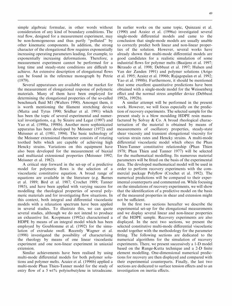
Very elastic materials sometimes snap back in anuncontrolled way after quick and large elongation. Aguiding pin, which is ®xed approximately 1 cm abovethe sample, has proved a useful tool to limit this risk, butsometimes one is simply forced to repeat the test toobtain a signi®cant result. Figure 1 shows a typicalexample of a retracting sample. It was obtained in anexperiment where the recovery phase evolves in accor-dance with the expectations.

50

Rheometric testing

A general-purpose blow moulding HDPE resin, basedon Ziegler-Natta catalyst technology, was appropriatelyoverstabilised and its stability was checked on a dynamicrheometer to exclude any interference of thermaldegradation on the recovery measurement. Sampleswere prepared by extrusion and subsequent recovery inan oil bath in order to remove frozen orientation. Allmeasurements were performed at 190 �C under anitrogen blanket.

The product was characterised using dynamicrheometry, in capillary and slit die rheometers, and withtransient stretching and subsequent recovery.

Dynamic rheometry

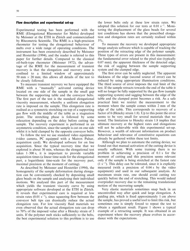
A ®rst step in the characterisation of the melt concernsthe linear viscoelastic properties and the shear viscosityas well. Here the product was characterised usingdynamic rheometry on an ARES rheometer from 10ÿ3to 100 sÿ1, in capillary and slit die rheometers. As isusual for HDPE melts the Cox-Merz rule appears to besatis®ed within experimental error. For this reason weshow and use only the dynamic measurement presentedin Fig. 2.

Transient elongational viscosity

Stretching and subsequent elongational recovery wereexplored on the RME under ten di�erent conditionsusing strain rates of 0.01, 0.1 and 1 sÿ1 and usingHencky ep strains 1, 2 and 3. The tenth measurement wasperformed at Hencky strain 4 using a strain rate of

0.1 sÿ1. Higher values of the Hencky strain were notconsidered due to additional experimental di�culties asbrie¯y discussed below. In several ®gures, the samplesare identi®ed by the pair strain rate j Hencky strain.

The elongational viscosity for all stretching measure-ments used in the analysis is shown in Fig. 3. The nicelyreproducible curves con®rm that our measurementwindow lies within an experimentally ``clean'' regionof testing conditions where necking is not observed. Infact at 0.01 sÿ1 this HDPE appears to be stretchable upto the limit of the instrument (Hencky strain 7 or anelongation factor of 1100) without breaking! Remark-able is the relatively high strain hardening level at lowstrain rates which is not uncommon for HDPE meltsbut is scarcely documented in the literature. This highstrain hardening level probably implies a pronouncedmaximum of the elongational viscosity curve as afunction of strain rate. Some examples are given byLaun and Schuch (1989), the di�erence here being thateven at 10ÿ3 sÿ1 no sign of an approach towards thelinear viscoelastic envelope can be detected. In fact, theregion where the curves could approach the envelopeappears to be experimentally inaccessible (the forcesbecome too small). Apart from the broad molecular

Fig. 1 Photograph of a retracting sample (strain rate � 1 sÿ1,Hencky strain � 2) at time t � 1.97 s after cutting. The actualsample length is 2.037 cm

Fig. 2 Linear viscoelastic properties of the high-density polyethylene(HDPE), measured at a temperature of 190 �C: experimentalmeasurements and model properties

51

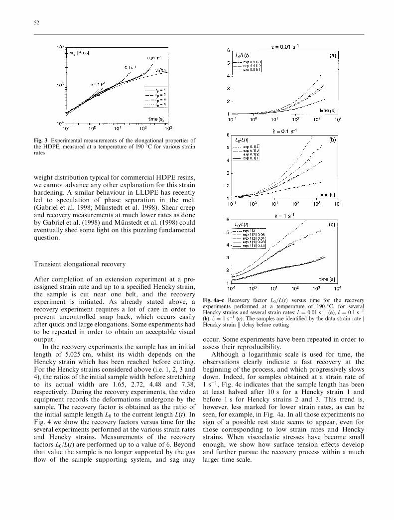
weight distribution typical for commercial HDPE resins,we cannot advance any other explanation for this strainhardening. A similar behaviour in LLDPE has recentlyled to speculation of phase separation in the melt(Gabriel et al. 1998; MuÈ nstedt et al. 1998). Shear creepand recovery measurements at much lower rates as doneby Gabriel et al. (1998) and MuÈ nstedt et al. (1998) couldeventually shed some light on this puzzling fundamentalquestion.

Transient elongational recovery

After completion of an extension experiment at a pre-assigned strain rate and up to a speci®ed Hencky strain,the sample is cut near one belt, and the recoveryexperiment is initiated. As already stated above, arecovery experiment requires a lot of care in order toprevent uncontrolled snap back, which occurs easilyafter quick and large elongations. Some experiments hadto be repeated in order to obtain an acceptable visualoutput.

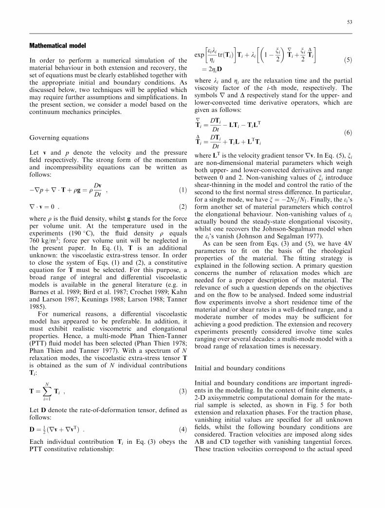
In the recovery experiments the sample has an initiallength of 5.025 cm, whilst its width depends on theHencky strain which has been reached before cutting.For the Hencky strains considered above (i.e. 1, 2, 3 and4), the ratios of the initial sample width before stretchingto its actual width are 1.65, 2.72, 4.48 and 7.38,respectively. During the recovery experiments, the videoequipment records the deformations undergone by thesample. The recovery factor is obtained as the ratio ofthe initial sample length L0 to the current length L(t). InFig. 4 we show the recovery factors versus time for theseveral experiments performed at the various strain ratesand Hencky strains. Measurements of the recoveryfactors L0/L(t) are performed up to a value of 6. Beyondthat value the sample is no longer supported by the gas¯ow of the sample supporting system, and sag may

occur. Some experiments have been repeated in order toassess their reproducibility.

Although a logarithmic scale is used for time, theobservations clearly indicate a fast recovery at thebeginning of the process, and which progressively slowsdown. Indeed, for samples obtained at a strain rate of1 sÿ1, Fig. 4c indicates that the sample length has beenat least halved after 10 s for a Hencky strain 1 andbefore 1 s for Hencky strains 2 and 3. This trend is,however, less marked for lower strain rates, as can beseen, for example, in Fig. 4a. In all those experiments nosign of a possible rest state seems to appear, even forthose corresponding to low strain rates and Henckystrains. When viscoelastic stresses have become smallenough, we show how surface tension e�ects developand further pursue the recovery process within a muchlarger time scale.

Fig. 3 Experimental measurements of the elongational properties ofthe HDPE, measured at a temperature of 190 �C for various strainrates

Fig. 4a±c Recovery factor L0=L�t� versus time for the recoveryexperiments performed at a temperature of 190 �C, for severalHencky strains and several strain rates: _e � 0.01 sÿ1 (a), _e � 0.1 sÿ1(b), _e � 1 sÿ1 (c). The samples are identi®ed by the data strain rate jHencky strain k delay before cutting

52

Mathematical model

In order to perform a numerical simulation of thematerial behaviour in both extension and recovery, theset of equations must be clearly established together withthe appropriate initial and boundary conditions. Asdiscussed below, two techniques will be applied whichmay require further assumptions and simpli®cations. Inthe present section, we consider a model based on thecontinuum mechanics principles.

Governing equations

Let v and p denote the velocity and the pressure®eld respectively. The strong form of the momentumand incompressibility equations can be written asfollows:

ÿrp �r � T� qg � qDv

Dt; �1�

r � v � 0 : �2�where q is the ¯uid density, whilst g stands for the forceper volume unit. At the temperature used in theexperiments (190 �C), the ¯uid density q equals760 kg/m3; force per volume unit will be neglected inthe present paper. In Eq. (1), T is an additionalunknown: the viscoelastic extra-stress tensor. In orderto close the system of Eqs. (1) and (2), a constitutiveequation for T must be selected. For this purpose, abroad range of integral and di�erential viscoelasticmodels is available in the general literature (e.g. inBarnes et al. 1989; Bird et al. 1987; Crochet 1989; Kahnand Larson 1987; Keunings 1988; Larson 1988; Tanner1985).

For numerical reasons, a di�erential viscoelasticmodel has appeared to be preferable. In addition, itmust exhibit realistic viscometric and elongationalproperties. Hence, a multi-mode Phan Thien-Tanner(PTT) ¯uid model has been selected (Phan Thien 1978;Phan Thien and Tanner 1977). With a spectrum of Nrelaxation modes, the viscoelastic extra-stress tensor Tis obtained as the sum of N individual contributionsTi:

T �XN

i�1Ti ; �3�

Let D denote the rate-of-deformation tensor, de®ned asfollows:

D � 12 �rv�rvT� : �4�

Each individual contribution Ti in Eq. (3) obeys thePTT constitutive relationship:

expeiki

gitr�Ti�

� �Ti � ki 1ÿ ni

2

� �Ti

r� ni

2Ti

D� �

� 2giD

�5�

where ki and gi are the relaxation time and the partialviscosity factor of the i-th mode, respectively. Thesymbols r and D respectively stand for the upper- andlower-convected time derivative operators, which aregiven as follows:

Ti

r� DTi

Dtÿ LTi ÿ TiL

T

Ti

D� DTi

Dt� TiL� LTTi

�6�

where LT is the velocity gradient tensorrv. In Eq. (5), niare non-dimensional material parameters which weighboth upper- and lower-convected derivatives and rangebetween 0 and 2. Non-vanishing values of ni introduceshear-thinning in the model and control the ratio of thesecond to the ®rst normal stress di�erence. In particular,for a single mode, we have n � ÿ2N2=N1. Finally, the ei'sform another set of material parameters which controlthe elongational behaviour. Non-vanishing values of eiactually bound the steady-state elongational viscosity,whilst one recovers the Johnson-Segalman model whenthe ei's vanish (Johnson and Segalman 1977).

As can be seen from Eqs. (3) and (5), we have 4Nparameters to ®t on the basis of the rheologicalproperties of the material. The ®tting strategy isexplained in the following section. A primary questionconcerns the number of relaxation modes which areneeded for a proper description of the material. Therelevance of such a question depends on the objectivesand on the ¯ow to be analysed. Indeed some industrial¯ow experiments involve a short residence time of thematerial and/or shear rates in a well-de®ned range, and amoderate number of modes may be su�cient forachieving a good prediction. The extension and recoveryexperiments presently considered involve time scalesranging over several decades: a multi-mode model with abroad range of relaxation times is necessary.

Initial and boundary conditions

Initial and boundary conditions are important ingredi-ents in the modelling. In the context of ®nite elements, a2-D axisymmetric computational domain for the mate-rial sample is selected, as shown in Fig. 5 for bothextension and relaxation phases. For the traction phase,vanishing initial values are speci®ed for all unknown®elds, whilst the following boundary conditions areconsidered. Traction velocities are imposed along sidesAB and CD together with vanishing tangential forces.These traction velocities correspond to the actual speed

53

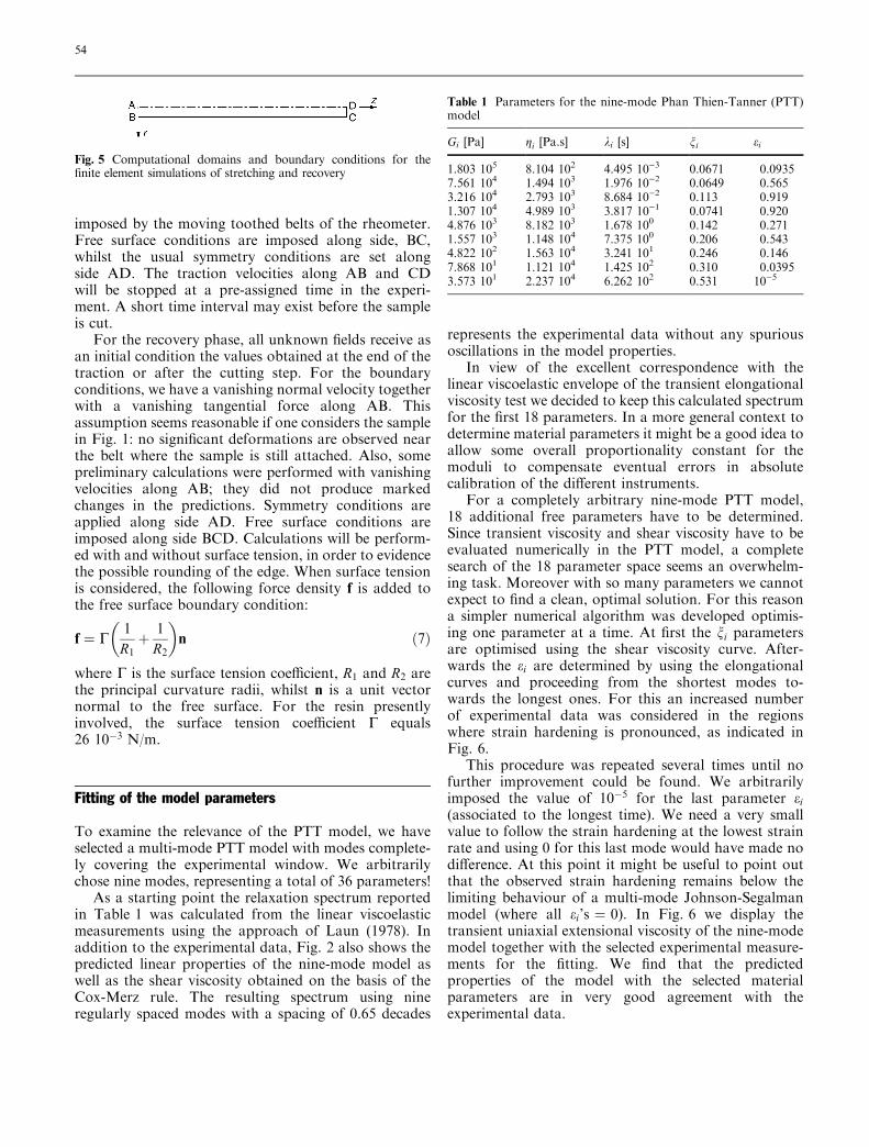
imposed by the moving toothed belts of the rheometer.Free surface conditions are imposed along side, BC,whilst the usual symmetry conditions are set alongside AD. The traction velocities along AB and CDwill be stopped at a pre-assigned time in the experi-ment. A short time interval may exist before the sampleis cut.

For the recovery phase, all unknown ®elds receive asan initial condition the values obtained at the end of thetraction or after the cutting step. For the boundaryconditions, we have a vanishing normal velocity togetherwith a vanishing tangential force along AB. Thisassumption seems reasonable if one considers the samplein Fig. 1: no signi®cant deformations are observed nearthe belt where the sample is still attached. Also, somepreliminary calculations were performed with vanishingvelocities along AB; they did not produce markedchanges in the predictions. Symmetry conditions areapplied along side AD. Free surface conditions areimposed along side BCD. Calculations will be perform-ed with and without surface tension, in order to evidencethe possible rounding of the edge. When surface tensionis considered, the following force density f is added tothe free surface boundary condition:

f � C1

R1� 1

R2

� �n �7�

where C is the surface tension coe�cient, R1 and R2 arethe principal curvature radii, whilst n is a unit vectornormal to the free surface. For the resin presentlyinvolved, the surface tension coe�cient C equals26 10ÿ3 N/m.

Fitting of the model parameters

To examine the relevance of the PTT model, we haveselected a multi-mode PTT model with modes complete-ly covering the experimental window. We arbitrarilychose nine modes, representing a total of 36 parameters!

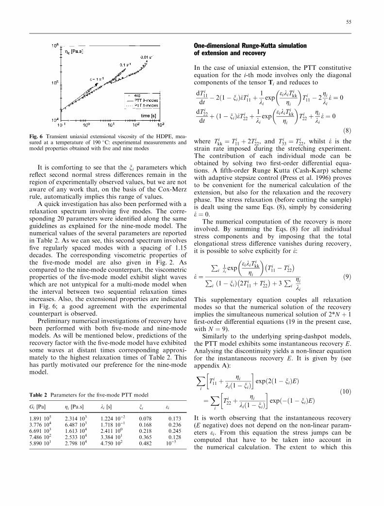
As a starting point the relaxation spectrum reportedin Table 1 was calculated from the linear viscoelasticmeasurements using the approach of Laun (1978). Inaddition to the experimental data, Fig. 2 also shows thepredicted linear properties of the nine-mode model aswell as the shear viscosity obtained on the basis of theCox-Merz rule. The resulting spectrum using nineregularly spaced modes with a spacing of 0.65 decades

represents the experimental data without any spuriousoscillations in the model properties.

In view of the excellent correspondence with thelinear viscoelastic envelope of the transient elongationalviscosity test we decided to keep this calculated spectrumfor the ®rst 18 parameters. In a more general context todetermine material parameters it might be a good idea toallow some overall proportionality constant for themoduli to compensate eventual errors in absolutecalibration of the di�erent instruments.

For a completely arbitrary nine-mode PTT model,18 additional free parameters have to be determined.Since transient viscosity and shear viscosity have to beevaluated numerically in the PTT model, a completesearch of the 18 parameter space seems an overwhelm-ing task. Moreover with so many parameters we cannotexpect to ®nd a clean, optimal solution. For this reasona simpler numerical algorithm was developed optimis-ing one parameter at a time. At ®rst the ni parametersare optimised using the shear viscosity curve. After-wards the ei are determined by using the elongationalcurves and proceeding from the shortest modes to-wards the longest ones. For this an increased numberof experimental data was considered in the regionswhere strain hardening is pronounced, as indicated inFig. 6.

This procedure was repeated several times until nofurther improvement could be found. We arbitrarilyimposed the value of 10ÿ5 for the last parameter ei(associated to the longest time). We need a very smallvalue to follow the strain hardening at the lowest strainrate and using 0 for this last mode would have made nodi�erence. At this point it might be useful to point outthat the observed strain hardening remains below thelimiting behaviour of a multi-mode Johnson-Segalmanmodel (where all ei's � 0). In Fig. 6 we display thetransient uniaxial extensional viscosity of the nine-modemodel together with the selected experimental measure-ments for the ®tting. We ®nd that the predictedproperties of the model with the selected materialparameters are in very good agreement with theexperimental data.

Fig. 5 Computational domains and boundary conditions for the®nite element simulations of stretching and recovery

Table 1 Parameters for the nine-mode Phan Thien-Tanner (PTT)model

Gi [Pa] gi [Pa.s] ki [s] ni ei

1.803 105 8.104 102 4.495 10)3 0.0671 0.09357.561 104 1.494 103 1.976 10)2 0.0649 0.5653.216 104 2.793 103 8.684 10)2 0.113 0.9191.307 104 4.989 103 3.817 10)1 0.0741 0.9204.876 103 8.182 103 1.678 100 0.142 0.2711.557 103 1.148 104 7.375 100 0.206 0.5434.822 102 1.563 104 3.241 101 0.246 0.1467.868 101 1.121 104 1.425 102 0.310 0.03953.573 101 2.237 104 6.262 102 0.531 10)5

54

It is comforting to see that the ni parameters whichre¯ect second normal stress di�erences remain in theregion of experimentally observed values, but we are notaware of any work that, on the basis of the Cox-Merzrule, automatically implies this range of values.

A quick investigation has also been performed with arelaxation spectrum involving ®ve modes. The corre-sponding 20 parameters were identi®ed along the sameguidelines as explained for the nine-mode model. Thenumerical values of the several parameters are reportedin Table 2. As we can see, this second spectrum involves®ve regularly spaced modes with a spacing of 1.15decades. The corresponding viscometric properties ofthe ®ve-mode model are also given in Fig. 2. Ascompared to the nine-mode counterpart, the viscometricproperties of the ®ve-mode model exhibit slight waveswhich are not untypical for a multi-mode model whenthe interval between two sequential relaxation timesincreases. Also, the extensional properties are indicatedin Fig. 6; a good agreement with the experimentalcounterpart is observed.

Preliminary numerical investigations of recovery havebeen performed with both ®ve-mode and nine-modemodels. As will be mentioned below, predictions of therecovery factor with the ®ve-mode model have exhibitedsome waves at distant times corresponding approxi-mately to the highest relaxation times of Table 2. Thishas partly motivated our preference for the nine-modemodel.

One-dimensional Runge-Kutta simulationof extension and recovery

In the case of uniaxial extension, the PTT constitutiveequation for the i-th mode involves only the diagonalcomponents of the tensor Ti and reduces to

dT i11

dtÿ 2�1ÿ ni� _eT i

11 �1

kiexp

eikiT ikk

gi

� �T i11 ÿ 2

gi

ki_e � 0

dT i22

dt� �1ÿ ni� _eT i

22 �1

kiexp

eikiT ikk

gi

� �T i22 �

gi

ki_e � 0

�8�where T i

kk � T i11 � 2T i

22, and T i33 � T i

22, whilst _e is thestrain rate imposed during the stretching experiment.The contribution of each individual mode can beobtained by solving two ®rst-order di�erential equa-tions. A ®fth-order Runge Kutta (Cash-Karp) schemewith adaptive stepsize control (Press et al. 1996) provesto be convenient for the numerical calculation of theextension, but also for the relaxation and the recoveryphase. The stress relaxation (before cutting the sample)is dealt using the same Eqs. (8), simply by considering_e � 0.

The numerical computation of the recovery is moreinvolved. By summing the Eqs. (8) for all individualstress components and by imposing that the totalelongational stress di�erence vanishes during recovery,it is possible to solve explicitly for _e:

_e �P

i1kiexp

eikiT ikk

gi

� �T i11 ÿ T i

22

ÿ �P

i �1ÿ ni� 2T i11 � T i

22

ÿ �� 3P

igi

ki

�9�

This supplementary equation couples all relaxationmodes so that the numerical solution of the recoveryimplies the simultaneous numerical solution of 2*N � 1®rst-order di�erential equations (19 in the present case,with N � 9).

Similarly to the underlying spring-dashpot models,the PTT model exhibits some instantaneous recovery E.Analysing the discontinuity yields a non-linear equationfor the instantaneous recovery E. It is given by (seeappendix A):X

i

T i11 �

gi

ki�1ÿ ni�� �

exp�2�1ÿ ni�E�

�X

i

T i22 �

gi

ki�1ÿ ni�� �

exp�ÿ�1ÿ ni�E��10�

It is worth observing that the instantaneous recovery(E negative) does not depend on the non-linear param-eters ei. From this equation the stress jumps can becomputed that have to be taken into account inthe numerical calculation. The extent to which this

Fig. 6 Transient uniaxial extensional viscosity of the HDPE, mea-sured at a temperature of 190 �C: experimental measurements andmodel properties obtained with ®ve and nine modes

Table 2 Parameters for the ®ve-mode PTT model

Gi [Pa] gi [Pa.s] ki [s] ni ei

1.891 105 2.314 103 1.224 10)2 0.078 0.1733.776 104 6.487 103 1.718 10)1 0.168 0.2366.691 103 1.613 104 2.411 100 0.218 0.2457.486 102 2.533 104 3.384 101 0.365 0.1285.890 101 2.798 104 4.750 102 0.482 10)5

55

instantaneous recovery becomes important dependsessentially on the choice of the relaxation spectrum. Abroad spectrum absorbs the instantaneous recovery. Inthe other limit, for a single relaxation mode all recoverywill be instantaneous.

Finite element method simulation

The mathematical developments displayed in the pre-vious section allow a quick solution to be obtained.However, the 1-D character of the above formulationmay hide some e�ects. For instance, it does not predictthe rounding at the edge due to surface tension. Whetherthose e�ects are meaningless or not cannot be assumedat the outset. It clearly depends on the material and a2-D axisymmetric calculation is therefore needed inorder to possibly validate some simplifying assumptions.

The ®nite element method will be used for solving theset of non-linear ¯ow governing equations along withthe speci®ed boundary conditions, in a 2-D axisymmet-ric geometry (Crochet et al. 1984; Keunings 1988). Forthis, we use the commercial ®nite element packagePOLYFLOW primarily designed for the analysis ofindustrial ¯ow situations dominated by non-linearviscous phenomena and viscoelastic e�ects (Crochetet al. 1992).

In the present work, we use the ®nite elementalgorithm referred to as the MIX1 method (Crochetet al. 1984; Van Schaftingen and Crochet 1984). In this®nite element method, easily extended to multi-modedi�erential viscoelastic models, all viscoelastic extra-stress components Ti and the velocity v are interpolatedby means of quadratic shape functions. The pressure p isrepresented by means of linear shape functions. Sincesurface tension e�ects are also considered, quadraticshape functions are also selected for the coordinates.

The MIX1 method has been extended to time-dependent viscoelastic ¯ows involving moving bound-aries by Keunings (1985), Bous®eld et al. (1986, 1988)and Keunings and Bous®eld (1987). By invoking theGalerkin formulation on deforming ®nite elements(Lynch and Gray 1980), a set of ®rst-order ordinarydi�erential equations is obtained which is then disc-retised in time by means of standard techniques (Josseand Finlayson 1984). The transient problem is solved bymeans of a predictor-corrector integration scheme wherethe corrector is the backward Euler method. The timestep is controlled along with the algorithm suggested byGresho et al. (1980, 1984). For time-integration, toler-ance criteria ranging from 10ÿ2 to 10ÿ5 are used, andhave led to solutions which, in most cases, could hardlybe distinguished from each other. It is worth mentioningthat a stability analysis of time-integration schemes forviscoelastic ¯ows has been performed by Bodart andCrochet (1993).

The ¯ow governing equations together with the freesurface condition are solved in a coupled fashion. Ateach time step, the Newton iterative scheme is appliedfor solving the non-linear algebraic system arising fromthe ®nite element discretisation. The non-linear iterationtermination is controlled by a speci®c iteration conver-gence criterion of 10ÿ4 for the relative error norms ofresiduals of the governing equations and free surfaceupdate. Spatial and temporal convergence of the simu-lation have been veri®ed separately.

An important ingredient for solving moving boun-dary problems is the remeshing algorithm which relo-cates internal nodes according to the displacement ofboundary nodes in order to avoid unacceptable elementdistortions. Two techniques will be applied according tothe situation. A spines technique similar to that devel-oped by Kistler and Scriven (1983) is applied for thetraction phase. In the recovery phase, we use theremeshing rule based on the Thompson transformation(Thompson et al. 1985). It consists of solving a partialdi�erential equation of the elliptic type for the coordi-nates, and it exhibits a high robustness even for verylarge mesh deformations. This has allowed performanceof recovery simulations for times as high as 104 s.

The geometric model used in this study is axisym-metric with respect to the central line. Consequently, inits initial con®guration, the axisymetric computationaldomain is de®ned by a rectangle. The computationaldomain is discretised by means of ®nite elements; twoslightly di�erent meshes have been used for performingthe several computations.

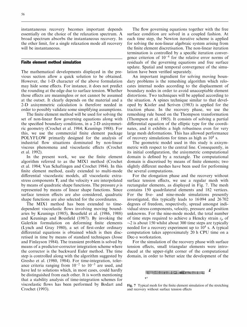
For the elongation phase and the recovery withoutsurface tension e�ects, we use a regular mesh withrectangular elements, as displayed in Fig. 7. The meshcontains 150 quadrilateral elements and 182 vertices.For the ®ve- and nine-mode simulations presentlyinvestigated, this typically leads to 16 094 and 26 702degrees of freedom, respectively, spread amongst indi-vidual stress components, velocity, pressure and positionunknowns. For the nine-mode model, the total numberof time steps required to achieve a Hencky strain ep of�2 is about 150 whilst about 300 time steps are typicallyneeded for a recovery experiment up to 104 s. A typicalcomputation takes approximately 20 h CPU time on aDec-a workstation.

For the simulation of the recovery phase with surfacetension e�ects, small triangular elements were intro-duced at the upper-right corner of the computationaldomain, in order to better seize the development of the

Fig. 7 Typical mesh for the ®nite element simulation of the stretchingand recovery without surface tension e�ects

56

rounding due to surface tension. A typical mesh isshown in Fig. 8: it contains 142 elements and 168vertices. For recovery simulations with the nine-modemodel, this leads to 24 768 degrees of freedom, alsospread amongst individual stress components, velocity,pressure and position unknowns.

One-dimensional simulations of recovery experiments

Mathematical models and numerical techniques havebeen set up in the above sections. In this section we wishto apply the 1-D calculation to several recoverysituations. Finite element results will be presented inthe following section. Extension simulations are per-formed before the recovery, in order to properly identifythe initial viscoelastic stresses. The extensions areperformed under the conditions given above: strainrates of 0.01, 0.1 and 1 sÿ1 are applied up to Henckystrains ep of 1, 2 and 3, whilst a tenth experiment at astrain rate of 0.1 sÿ1 is performed up to a Hencky strainof 4. The corresponding times involved for all theseexperiments are obtained as the ratio of the Henckystrain to the strain rate.

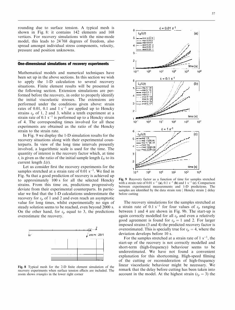
In Fig. 9 we display the 1-D simulation results for therecovery situations along with their experimental coun-terparts. In view of the long time intervals presentlyinvolved, a logarithmic scale is used for the time. Thequantity of interest is the recovery factor which, at timet, is given as the ratio of the initial sample length L0 to itscurrent length L(t).

Let us consider ®rst the recovery experiments for thesamples stretched at a strain rate of 0.01 sÿ1. We ®nd inFig. 9a that a good prediction of recovery is achieved upto approximately 100 s for all the selected Henckystrains. From this time on, predictions progressivelydeviate from their experimental counterparts. In partic-ular we ®nd that the 1-D calculations underestimate therecovery for ep of 1 and 2 and even reach an asymptoticvalue for long times, whilst experimentally no sign ofsteady solution seems to be reached, even beyond 2000 s.On the other hand, for ep equal to 3, the predictionsoverestimate the recovery.

The recovery simulations for the samples stretched ata strain rate of 0.1 sÿ1 for four values of ep rangingbetween 1 and 4 are shown in Fig. 9b. The start-up isagain correctly modelled for all ep and even a relativelygood agreement is found for ep � 1 and 2. For largerimposed strains (3 and 4) the predicted recovery factor isoverestimated. This is specially true for ep � 4, where thedeviation develops before 10 s.

For the samples stretched at a strain rate of 1 sÿ1, thestart-up of the recovery is not correctly modelled andshort-term (high-frequency) behaviour seems to beunderestimated. We have not found a convenientexplanation for this shortcoming. High-speed ®lmingof the cutting or reconsideration of high-frequencylinear viscoelastic behaviour might be necessary. Weremark that the delay before cutting has been taken intoaccount in the model. At the highest strain (ep � 3) the

Fig. 8 Typical mesh for the 2-D ®nite element simulation of therecovery experiments when surface tension e�ects are included. Thezoom shows triangles in the lower right corner

Fig. 9 Recovery factor as a function of time for samples stretchedwith a strain rate of 0.01 sÿ1 (a), 0.1 sÿ1 (b) and 1 sÿ1 (c). Comparisonbetween experimental measurements and 1-D predictions. Thesamples are identi®ed by the data strain rate j Hencky strain k delaybefore cutting

57

recovery predictions again overestimate the experimen-tal counterparts after 30 s.

Despite the observed deviations between simulationsand measurements, it is remarkable that the samequalitative trend is found for all cases. Indeed, in thedisplayed diagrams with a logarithmic scale for time t,the recovery curves for samples stretched at 0.01 and0.1 sÿ1 exhibit an upward oriented concavity in bothpredictions and experiments.

The observed deviations between simulations andmeasurements may have several origins. For low strainrates, viscoelastic stresses are relatively low, and surfacetension e�ects may progressively develop as stressesfade, as will be shown in the next section. In particular,it will be shown that recovery is further pursued withsurface tension e�ects.

By modelling the in¯uence of short elapsed timeintervals between the end of stretching and the momentof cutting, we can exclude the possibility that thedeviations observed at high Hencky strains may havetheir origin in the cutting process.

The deviations at high Hencky strains might possiblyhave their origin in an irreversible mechanism ofmolecular disentanglement due to the high (and fast)deformations undergone by the sample during thestretching phase. The presently selected constitutivemodel probably does not contain the best appropriateirreversible mechanism that would be needed in certaincircumstances. The selection of an integral viscoelasticconstitutive equation with an irreversible dampingfunction could probably be a remedy; unfortunatelythe use of such a model for simulating general time-dependent 2-D ¯ows would be endowed with seriouscomputational challenges. Actually, we believe that inthe context of di�erential viscoelastic models, it ispossible to develop equations that would be capable ofproducing a more pronounced irreversible mechanism.New models can be developed along the guidelinesdrawn up, for example, by Suovaliotis and Beris (1992)and Edwards et al. (1996). Quite obviously, this is achallenge addressed to rheologists.

Surface tension effects

In the results displayed in the previous section, surfacetension e�ects have been neglected. At ®rst, thisassumption seems to be reasonable. Indeed, althoughthe samples are geometrically characterised by smalldimensions, viscoelastic stresses in the melt are severalorders of magnitude larger than surface tension. How-ever, the recovery occurs within a long time interval, sothat possible surface tension e�ects may eventuallydevelop, leading in particular to the rounding of thesharp edge at the cutting location. In order to verify ourinitial assumption of negligible surface tension, we

presently intend to review three recovery simulationsperformed above. For this, we select the samplesobtained in the elongation experiments performed (1)at a strain rate of 0.01 sÿ1 up to a Hencky strain of 3, (2)at a strain rate of 0.1 sÿ1 up to a Hencky strain of 1, and(3) at a strain rate of 1 sÿ1 up to a Hencky strain of 2.Those samples are obtained after a stretching time of300, 10 and 2 s, respectively. For performing such asimulation, the possible non-uniform deformationsrequire the use of the 2-D axisymmetric ®nite elementmethod, as described above.

In its initial con®guration in the recovery experi-ments, the samples have a length of 5.025 cm and aradius of 0.053, 0.143 and 0.087 cm, respectively. Alsothe values of all individual components of the viscoelas-tic stress tensor T and of the pressure as obtained at theend of the elongation are used as initial conditions forthe recovery simulation.

The recovery simulation is performed during a timeinterval of 104 s. In Fig. 10, we display on a logarithmicplot the recovery as a function of time, obtained for allthree samples presently considered; simultaneously wedisplay the 1-D simulation results and the experimentalcounterparts. We observe that surface tension starts todevelop after 100 s, and its e�ects are quite visible afterabout 500 s. Without surface tension, the recoveryceases after about 2000 s, whilst it is pursued andenhanced by surface tension. At low Hencky strain(second sample), a good agreement is found between the®nite element predictions and their experimental coun-terpart. However, for the highest Hencky strains (3 or 4)the deviation between experiments and calculations isenhanced by surface tension e�ects. Yet, in all cases, thesame qualitative trend is observed in terms of recoveryfactor growth for long times.

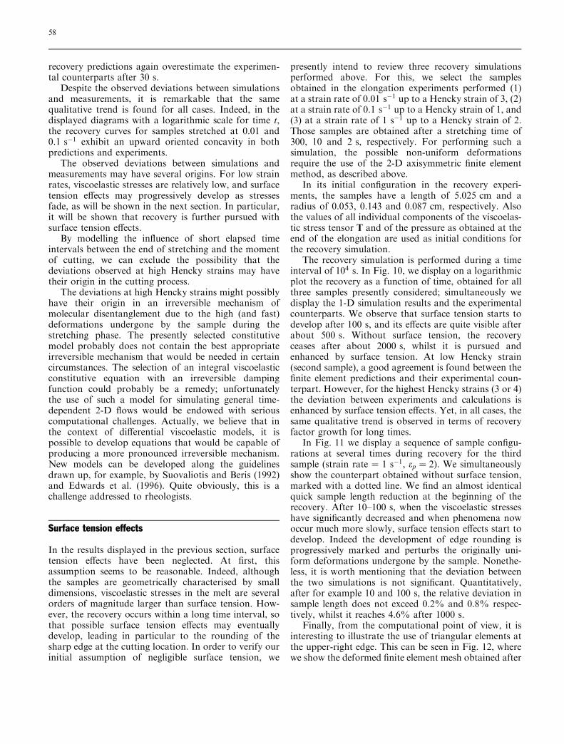
In Fig. 11 we display a sequence of sample con®gu-rations at several times during recovery for the thirdsample (strain rate � 1 sÿ1, ep � 2). We simultaneouslyshow the counterpart obtained without surface tension,marked with a dotted line. We ®nd an almost identicalquick sample length reduction at the beginning of therecovery. After 10±100 s, when the viscoelastic stresseshave signi®cantly decreased and when phenomena nowoccur much more slowly, surface tension e�ects start todevelop. Indeed the development of edge rounding isprogressively marked and perturbs the originally uni-form deformations undergone by the sample. Nonethe-less, it is worth mentioning that the deviation betweenthe two simulations is not signi®cant. Quantitatively,after for example 10 and 100 s, the relative deviation insample length does not exceed 0.2% and 0.8% respec-tively, whilst it reaches 4.6% after 1000 s.

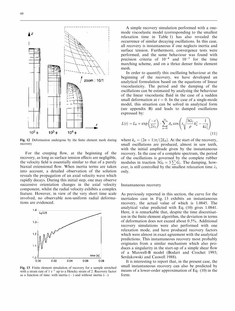
Finally, from the computational point of view, it isinteresting to illustrate the use of triangular elements atthe upper-right edge. This can be seen in Fig. 12, wherewe show the deformed ®nite element mesh obtained after

58

102, 103 and 104 s in the third recovery experiment.A zoom has been displayed near the rounded edgeobtained at time t � 104 s. If one refers to the initial®nite element mesh shown in Fig. 8, we ®nd that elementskewing is quite visible. Preliminary simulations haveshown that the use of quadrilaterals at the edge did notallow really satisfactory results to be obtained.

Inertia effects ± instantaneous recovery

Combined e�ects of rheological model and inertia

The ®nite element simulation of the recovery experimentfor the sample stretched with a strain rate of 1 sÿ1 up to

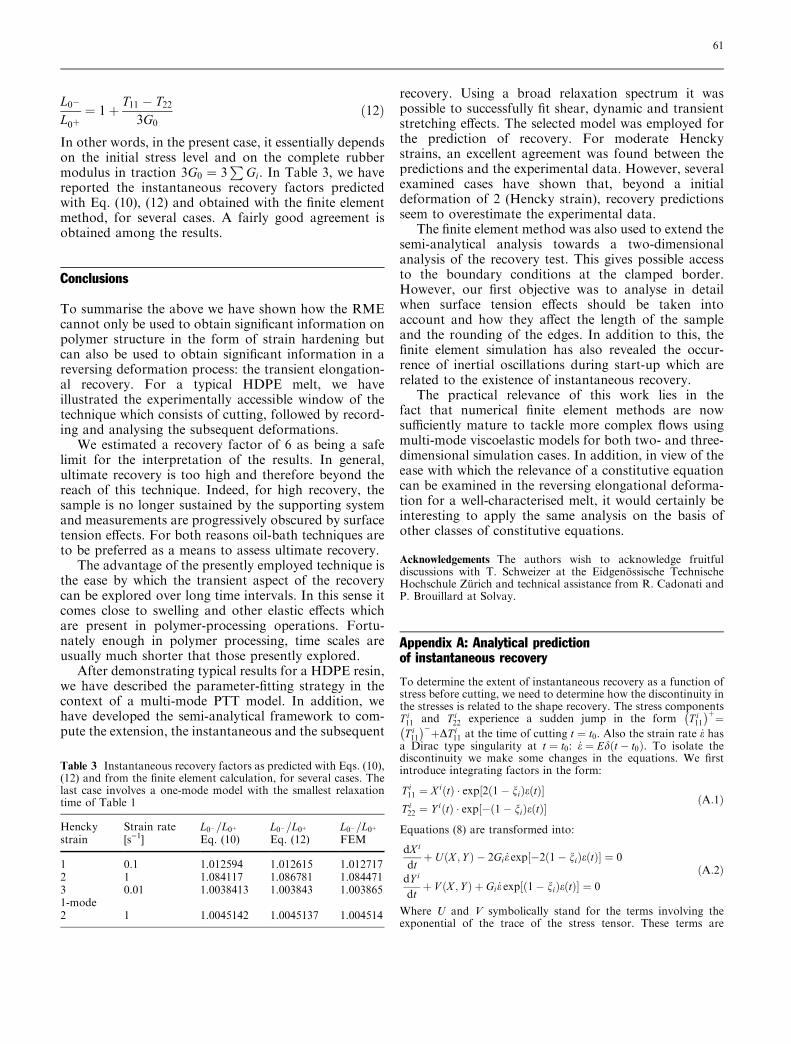
a Hencky strain of 2 has revealed the occurrence ofoscillations in the recovery factor. This feature needed tobe further investigated. The recovery simulation wasperformed anew with a precision criterion of 10ÿ4 for thetime marching scheme, leading to a tremendous numberof time steps. In Fig. 13 we display the recovery as afunction of time during the ®rst time interval of 0.08 s.Here, we clearly see the oscillating behaviour whichrapidly decays on the time scale of the smallestrelaxation time given in Table 1.

Those oscillations originate from the combination ofinertia e�ects and instantaneous recovery. Indeed,simulations performed without inertia have shown theoccurrence of an instantaneous recovery, but did notexhibit any oscillations, as can be seen on the dashedrecovery curve displayed in Fig. 13. In addition, the tworecovery curves obtained with an without inertia mergebeyond approximately 0.04 s. Actually the creeping ¯owmodel obeys a non-linear system of PD equations of the®rst order, and as stated above, the 1-D solution for thecreeping ¯ow exhibits a singularity at the initial time ofthe recovery. This is also found on the recovery curve forthe inertialess case in Fig. 13 obtained with ®niteelements, where we may easily observe the occurrenceof an instantaneous recovery. The introduction of arelatively low inertial contribution, thus of a second-order derivative, can be viewed as a perturbation of theinitially ®rst-order system of equations.

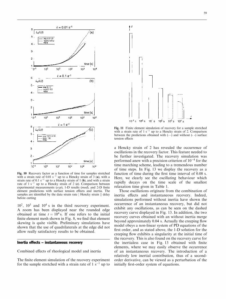
Fig. 10 Recovery factor as a function of time for samples stretchedwith a strain rate of 0.01 sÿ1 up to a Hencky strain of 3 (a), with astrain rate of 0.1 sÿ1 up to a Hencky strain of 1 (b), and with a strainrate of 1 sÿ1 up to a Hencky strain of 2 (c). Comparison betweenexperimental measurements (exp), 1-D results (mod), and 2-D ®niteelement predictions with surface tension e�ects and inertia. Thesamples are identi®ed by the data strain rate j Hencky strain k delaybefore cutting

Fig. 11 Finite element simulation of recovery for a sample stretchedwith a strain rate of 1 sÿ1 up to a Hencky strain of 2. Comparisonbetween the predictions obtained with (Ð) and without (- -) surfacetension e�ects

59

For the creeping ¯ow, at the beginning of therecovery, as long as surface tension e�ects are negligible,the velocity ®eld is essentially similar to that of a purelybiaxial extensional ¯ow. When inertia terms are takeninto account, a detailed observation of the solutionreveals the propagation of an axial velocity wave whichrapidly decays. During this initial step, one may observesuccessive orientation changes in the axial velocitycomponent, whilst the radial velocity exhibits a complexfeature. However, in view of the very short time scaleinvolved, no observable non-uniform radial deforma-tions are evidenced.

A simple recovery simulation performed with a one-mode viscoelastic model (corresponding to the smallestrelaxation time in Table 1) has also revealed theoccurrence of similar decaying oscillations. In this case,all recovery is instantaneous if one neglects inertia andsurface tension. Furthermore, convergence tests wereperformed, and the same behaviour was found withprecision criteria of 10ÿ4 and 10ÿ5 for the timemarching scheme, and on a thrice denser ®nite elementmesh.

In order to quantify this oscillating behaviour at thebeginning of the recovery, we have developed ananalytical formulation based on the equations of linearviscoelasticity. The period and the damping of theoscillations can be estimated by analysing the behaviourof the linear viscoelastic ¯uid in the case of a suddensmall deformation at t � 0. In the case of a single-modemodel, this situation can be solved in analytical form(see appendix B) and leads to damped oscillationsexpressed by:

L�t� � L0 � expÿt2k1

� ��X1n�0

An cos t

��������������������������3G1

qk2n ÿ

1

4k21

s !�11�

where kn � �2n� 1�p=�2L0�. At the start of the recovery,small oscillations are produced, almost in saw teeth,with the initial amplitude given by the instantaneousrecovery. In the case of a complete spectrum, the periodof the oscillations is governed by the complete rubbermodulus in traction 3G0 � 3

PGi. The damping, how-

ever, is still controlled by the smallest relaxation time k1only.

Instantaneous recovery

As previously reported in this section, the curve for theinertialess case in Fig. 13 exhibits an instantaneousrecovery, the actual value of which is 1.0845. Theanalytical value predicted with Eq. (10) gives 1.0841.Here, it is remarkable that, despite the time discretisat-ion in the ®nite element algorithm, the deviation in termsof deformation does not exceed about 0.5%. Additionalrecovery simulations were also performed with onerelaxation mode, and have produced recovery factorswhich were almost in exact agreement with the analyticalpredictions. This instantaneous recovery most probablyoriginates from a similar mechanism which also pro-duces a singularity in the start-up of a simple shear ¯owof a Maxwell-B model (Bodart and Crochet 1993;Serdakowski and Caswell 1988).

It is interesting to report that, in the present case, thesmall instantaneous recovery can also be predicted bymeans of a lower-order approximation of Eq. (10) in theform:

Fig. 12 Deformation undergone by the ®nite element mesh duringrecovery

Fig. 13 Finite element simulation of recovery for a sample stretchedwith a strain rate of 1 sÿ1 up to a Hencky strain of 2. Recovery factoras a function of time: with inertia (Ð) and without inertia (- -)

60

L0ÿL0�� 1� T11 ÿ T22

3G0�12�

In other words, in the present case, it essentially dependson the initial stress level and on the complete rubbermodulus in traction 3G0 � 3

PGi. In Table 3, we have

reported the instantaneous recovery factors predictedwith Eq. (10), (12) and obtained with the ®nite elementmethod, for several cases. A fairly good agreement isobtained among the results.

Conclusions

To summarise the above we have shown how the RMEcannot only be used to obtain signi®cant information onpolymer structure in the form of strain hardening butcan also be used to obtain signi®cant information in areversing deformation process: the transient elongation-al recovery. For a typical HDPE melt, we haveillustrated the experimentally accessible window of thetechnique which consists of cutting, followed by record-ing and analysing the subsequent deformations.

We estimated a recovery factor of 6 as being a safelimit for the interpretation of the results. In general,ultimate recovery is too high and therefore beyond thereach of this technique. Indeed, for high recovery, thesample is no longer sustained by the supporting systemand measurements are progressively obscured by surfacetension e�ects. For both reasons oil-bath techniques areto be preferred as a means to assess ultimate recovery.

The advantage of the presently employed technique isthe ease by which the transient aspect of the recoverycan be explored over long time intervals. In this sense itcomes close to swelling and other elastic e�ects whichare present in polymer-processing operations. Fortu-nately enough in polymer processing, time scales areusually much shorter that those presently explored.

After demonstrating typical results for a HDPE resin,we have described the parameter-®tting strategy in thecontext of a multi-mode PTT model. In addition, wehave developed the semi-analytical framework to com-pute the extension, the instantaneous and the subsequent

recovery. Using a broad relaxation spectrum it waspossible to successfully ®t shear, dynamic and transientstretching e�ects. The selected model was employed forthe prediction of recovery. For moderate Henckystrains, an excellent agreement was found between thepredictions and the experimental data. However, severalexamined cases have shown that, beyond a initialdeformation of 2 (Hencky strain), recovery predictionsseem to overestimate the experimental data.

The ®nite element method was also used to extend thesemi-analytical analysis towards a two-dimensionalanalysis of the recovery test. This gives possible accessto the boundary conditions at the clamped border.However, our ®rst objective was to analyse in detailwhen surface tension e�ects should be taken intoaccount and how they a�ect the length of the sampleand the rounding of the edges. In addition to this, the®nite element simulation has also revealed the occur-rence of inertial oscillations during start-up which arerelated to the existence of instantaneous recovery.

The practical relevance of this work lies in thefact that numerical ®nite element methods are nowsu�ciently mature to tackle more complex ¯ows usingmulti-mode viscoelastic models for both two- and three-dimensional simulation cases. In addition, in view of theease with which the relevance of a constitutive equationcan be examined in the reversing elongational deforma-tion for a well-characterised melt, it would certainly beinteresting to apply the same analysis on the basis ofother classes of constitutive equations.

Acknowledgements The authors wish to acknowledge fruitfuldiscussions with T. Schweizer at the EidgenoÈ ssische TechnischeHochschule ZuÈ rich and technical assistance from R. Cadonati andP. Brouillard at Solvay.

Appendix A: Analytical predictionof instantaneous recovery

To determine the extent of instantaneous recovery as a function ofstress before cutting, we need to determine how the discontinuity inthe stresses is related to the shape recovery. The stress componentsT i11 and T i

22 experience a sudden jump in the form T i11

ÿ ���T i11

ÿ �ÿ�DT i11 at the time of cutting t � t0. Also the strain rate _e has

a Dirac type singularity at t � t0: _e � Ed�t ÿ t0�. To isolate thediscontinuity we make some changes in the equations. We ®rstintroduce integrating factors in the form:

T i11 � X i�t� � exp�2�1ÿ ni�e�t��

T i22 � Y i�t� � exp�ÿ�1ÿ ni�e�t��

�A:1�

Equations (8) are transformed into:

dX i

dt� U�X ; Y � ÿ 2Gi _e exp�ÿ2�1ÿ ni�e�t�� � 0

dY i

dt� V �X ; Y � � Gi _e exp��1ÿ ni�e�t�� � 0

�A:2�

Where U and V symbolically stand for the terms involving theexponential of the trace of the stress tensor. These terms are

Table 3 Instantaneous recovery factors as predicted with Eqs. (10),(12) and from the ®nite element calculation, for several cases. Thelast case involves a one-mode model with the smallest relaxationtime of Table 1

Henckystrain

Strain rate[s)1]

L0ÿ=L0�

Eq. (10)L0ÿ=L0�

Eq. (12)L0ÿ=L0�

FEM

1 0.1 1.012594 1.012615 1.0127172 1 1.084117 1.086781 1.0844713 0.01 1.0038413 1.003843 1.0038651-mode2 1 1.0045142 1.0045137 1.004514

61

discontinuous but not singular at t � t0. Equations (A.2) can berewritten as:

d

dtX i � Gi

�1ÿ ni�exp�ÿ2�1ÿ ni�e�t��

� �� U�X ; Y � � 0

d

dtY i � Gi

�1ÿ ni�exp��1ÿ ni�e�t��

� �� V �X ; Y � � 0

�A:3�

By formally integrating the equations (A.3) from 0 to t whileintroducing integration constants Ki and Li and by using thede®nitions (A.1), we ®nd:

T i11 �

Gi

�1ÿ ni�� Ki �

Z t

0

~U�T11; T22� dt� �

exp�2�1ÿ ni�e�t��

T i22 �

Gi

�1ÿ ni�� Li �

Z t

0

~V �T11; T22� dt� �

exp�ÿ�1ÿ ni�e�t��

�A:4�

where we have introduced ~U and ~V to represent both U and V as afunction of the stresses. Those developments have isolated thecomplete stress discontinuity as a prefactor. If the strain experi-ences a jump E at t � t0, we ®nd:

T i11 �

Gi

�1ÿ ni�� �

�t0��

� exp�2�1ÿ ni�E� T i11 �

Gi

�1ÿ ni�� �

�t0ÿ�

T i22 �

Gi

�1ÿ ni�� �

�t0��

� exp�ÿ�1ÿ ni�E� T i22 �

Gi

�1ÿ ni�� �

�t0ÿ�

�A:5�

The strain jump can now to computed by imposing isotropy of thestresses after shape recovery. This amounts to setting:X

i

T i11 �

Gi

�1ÿ ni�� �

�t0��

�X

i

T i22 �

Gi

�1ÿ ni�� �

�t0���A:6�

which ®nally results in a relationship involving E and the stresses atthe end of streching:X

i

T i11 �

Gi

�1ÿ ni�� �

exp�2�1ÿ ni�E�

�X

i

T i22 �

Gi

�1ÿ ni�� �

exp�ÿ�1ÿ ni�E��A:7�

Appendix B: Analytical formulae for inertial oscillations

The basic assumptions are as follows:

1. Inertial e�ects are coupled to the non-homogeneous deforma-tions which occur during nearly instantaneous recovery: we donot need to consider the previous homogeneous stress history. Itis equivalent to impose a sudden traction with the samemagnitude as the instantaneous recovery, immediately followedby instantaneous recovery.

2. This instantaneous recovery is small and can be treated in theframework of linear viscoelasticity.

3. The geometry is almost one-dimensional; in other words, weconsider a rod with a radius to length ratio much lower thanunity.

The model is described in a coordinate system associated with theequilibrium position, with 0 � z � L0. At time t � 0, the sample isstreched up to a length L, with L=L0 � a. Hence, in the completemodel, a is the instantaneous contribution to the deformation.

The momentum equation along the axial direction of the rodcan be written in terms of a small displacement as follows:

q�uÿ 3GZ t

0ÿeÿ�tÿs�=k o2 _u�z; s�

oz2ds � 0 �B:1�

where 3G is the rubber modulus in traction. As the initial conditionwe have u�z; 0� � �aÿ 1�z. For the boundary conditions, we have:

u�0; t� � 0 ;

o _u�z; t�oz

� 0 for z � L0 :�B:2�

To solve Eq. (B.1) we have constructed an auxiliary function g�z; t�in the form of a series of An � ejxnt � sin�knz� which satis®es equation(B.1) with g�0; t� � 0 and og�z; t�=oz � 0 for z � L0. This implies:

kn � �2n� 1�p=�2L0� �B:3�If we consider that

g�z� �X1n�0

An � sin�knz�

�initial condition at t � 0��B:4�

we ®nd that

g�z; t� �X1n�0

An � ejxnt � sin�knz� �B:5�

is a solution of Eq. (B.1) provided that:

xn � j2k�

������������������������3Gq

k2n ÿ1

4k2

s�B:6�

and that

3Gq

o2g�z�oz2

� 1

2k2g�z� � 0 �B:7�

With Eq. (B.7), we ®nd:

g�z� � D � sin�bz�; with b � 1

2k

������2q3G

r�B:8�

Using the auxiliary function g(z,t) we can now construct thesolution of the original equation (B.1) as:

u�z; t� � �aÿ 1�zÿ g�z� � g�z; t� �B:9�The value of D is set by requiring that u�L0; t� � 0 for t � 1,Finally, we obtain:

g�z� � �aÿ 1�L0

sin�bL0� � sin�bz� �B:10�

Finally, the complete solution can be written as:

u�z; t� � �aÿ 1�zÿ �aÿ 1�L0

sin�bL0� � sin�bz�

�X1n�0

An:ejxnt:sin�knz��B:11�

62

with kn and xn respectively given by (B.3) and (B.6) and with

An � 2�aÿ 1�sin�bL0�

� sin��bÿ kn�L0�bÿ kn

ÿ sin��b� kn�L0�b� kn

� � �B:12�

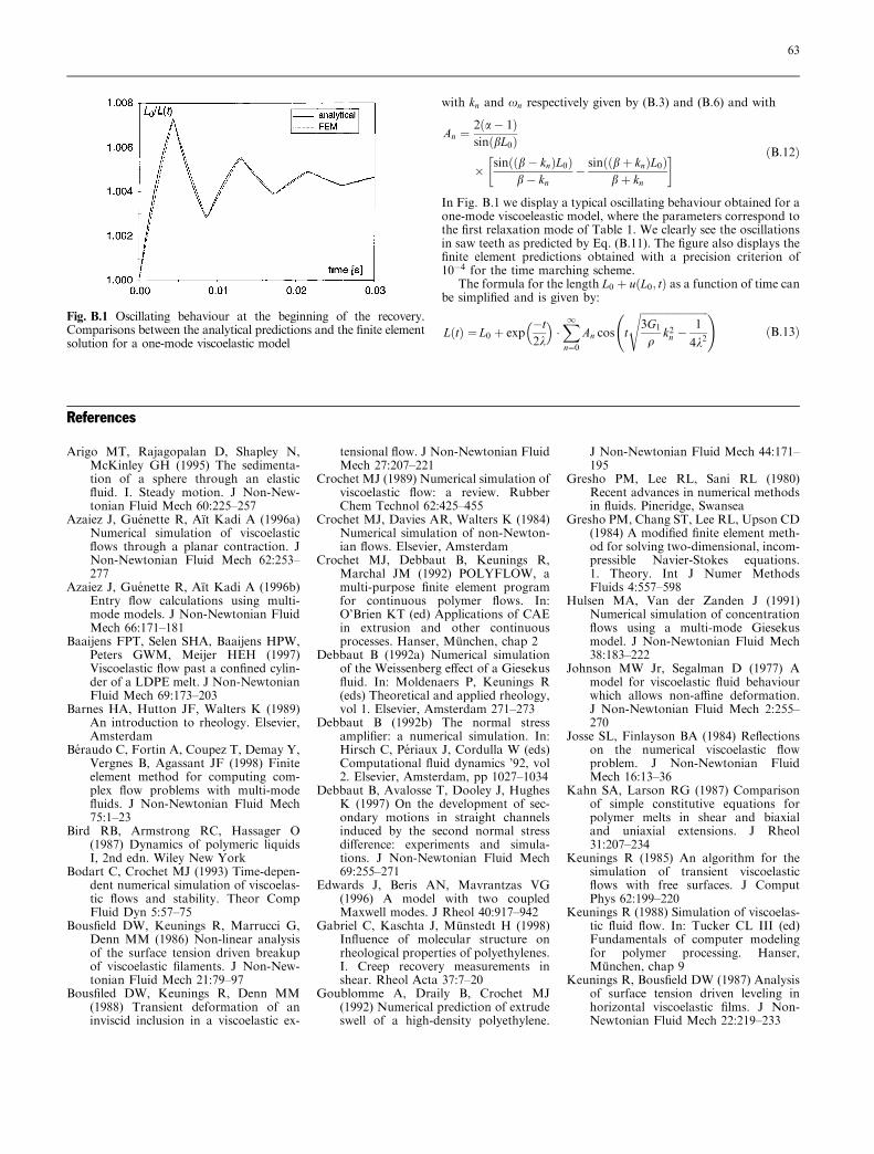
In Fig. B.1 we display a typical oscillating behaviour obtained for aone-mode viscoeleastic model, where the parameters correspond tothe ®rst relaxation mode of Table 1. We clearly see the oscillationsin saw teeth as predicted by Eq. (B.11). The ®gure also displays the®nite element predictions obtained with a precision criterion of10ÿ4 for the time marching scheme.

The formula for the length L0 � u�L0; t� as a function of time canbe simpli®ed and is given by:

L�t� � L0 � expÿt2k

� ��X1n�0

An cos t

��������������������������3G1

qk2n ÿ

1

4k2

s !�B:13�

References

Arigo MT, Rajagopalan D, Shapley N,McKinley GH (1995) The sedimenta-tion of a sphere through an elastic¯uid. I. Steady motion. J Non-New-tonian Fluid Mech 60:225±257

Azaiez J, Gue nette R, AõÈ t Kadi A (1996a)Numerical simulation of viscoelastic¯ows through a planar contraction. JNon-Newtonian Fluid Mech 62:253±277

Azaiez J, Gue nette R, AõÈ t Kadi A (1996b)Entry ¯ow calculations using multi-mode models. J Non-Newtonian FluidMech 66:171±181

Baaijens FPT, Selen SHA, Baaijens HPW,Peters GWM, Meijer HEH (1997)Viscoelastic ¯ow past a con®ned cylin-der of a LDPE melt. J Non-NewtonianFluid Mech 69:173±203

Barnes HA, Hutton JF, Walters K (1989)An introduction to rheology. Elsevier,Amsterdam

Be raudo C, Fortin A, Coupez T, Demay Y,Vergnes B, Agassant JF (1998) Finiteelement method for computing com-plex ¯ow problems with multi-mode¯uids. J Non-Newtonian Fluid Mech75:1±23

Bird RB, Armstrong RC, Hassager O(1987) Dynamics of polymeric liquidsI, 2nd edn. Wiley New York

Bodart C, Crochet MJ (1993) Time-depen-dent numerical simulation of viscoelas-tic ¯ows and stability. Theor CompFluid Dyn 5:57±75

Bous®eld DW, Keunings R, Marrucci G,Denn MM (1986) Non-linear analysisof the surface tension driven breakupof viscoelastic ®laments. J Non-New-tonian Fluid Mech 21:79±97

Bous®led DW, Keunings R, Denn MM(1988) Transient deformation of aninviscid inclusion in a viscoelastic ex-

tensional ¯ow. J Non-Newtonian FluidMech 27:207±221

Crochet MJ (1989) Numerical simulation ofviscoelastic ¯ow: a review. RubberChem Technol 62:425±455

Crochet MJ, Davies AR, Walters K (1984)Numerical simulation of non-Newton-ian ¯ows. Elsevier, Amsterdam

Crochet MJ, Debbaut B, Keunings R,Marchal JM (1992) POLYFLOW, amulti-purpose ®nite element programfor continuous polymer ¯ows. In:O'Brien KT (ed) Applications of CAEin extrusion and other continuousprocesses. Hanser, MuÈ nchen, chap 2

Debbaut B (1992a) Numerical simulationof the Weissenberg e�ect of a Giesekus¯uid. In: Moldenaers P, Keunings R(eds) Theoretical and applied rheology,vol 1. Elsevier, Amsterdam 271±273

Debbaut B (1992b) The normal stressampli®er: a numerical simulation. In:Hirsch C, Pe riaux J, Cordulla W (eds)Computational ¯uid dynamics '92, vol2. Elsevier, Amsterdam, pp 1027±1034

Debbaut B, Avalosse T, Dooley J, HughesK (1997) On the development of sec-ondary motions in straight channelsinduced by the second normal stressdi�erence: experiments and simula-tions. J Non-Newtonian Fluid Mech69:255±271

Edwards J, Beris AN, Mavrantzas VG(1996) A model with two coupledMaxwell modes. J Rheol 40:917±942

Gabriel C, Kaschta J, MuÈ nstedt H (1998)In¯uence of molecular structure onrheological properties of polyethylenes.I. Creep recovery measurements inshear. Rheol Acta 37:7±20

Goublomme A, Draily B, Crochet MJ(1992) Numerical prediction of extrudeswell of a high-density polyethylene.

J Non-Newtonian Fluid Mech 44:171±195

Gresho PM, Lee RL, Sani RL (1980)Recent advances in numerical methodsin ¯uids. Pineridge, Swansea

Gresho PM, Chang ST, Lee RL, Upson CD(1984) A modi®ed ®nite element meth-od for solving two-dimensional, incom-pressible Navier-Stokes equations.1. Theory. Int J Numer MethodsFluids 4:557±598

Hulsen MA, Van der Zanden J (1991)Numerical simulation of concentration¯ows using a multi-mode Giesekusmodel. J Non-Newtonian Fluid Mech38:183±222

Johnson MW Jr, Segalman D (1977) Amodel for viscoelastic ¯uid behaviourwhich allows non-a�ne deformation.J Non-Newtonian Fluid Mech 2:255±270

Josse SL, Finlayson BA (1984) Re¯ectionson the numerical viscoelastic ¯owproblem. J Non-Newtonian FluidMech 16:13±36

Kahn SA, Larson RG (1987) Comparisonof simple constitutive equations forpolymer melts in shear and biaxialand uniaxial extensions. J Rheol31:207±234

Keunings R (1985) An algorithm for thesimulation of transient viscoelastic¯ows with free surfaces. J ComputPhys 62:199±220

Keunings R (1988) Simulation of viscoelas-tic ¯uid ¯ow. In: Tucker CL III (ed)Fundamentals of computer modelingfor polymer processing. Hanser,MuÈ nchen, chap 9

Keunings R, Bous®eld DW (1987) Analysisof surface tension driven leveling inhorizontal viscoelastic ®lms. J Non-Newtonian Fluid Mech 22:219±233

Fig. B.1 Oscillating behaviour at the beginning of the recovery.Comparisons between the analytical predictions and the ®nite elementsolution for a one-mode viscoelastic model

63

Kistler SF, Scriven LE (1983) Coating¯ows. In: Pearson JRA, RichardsonSM (eds), Computational analysis ofpolymer processing. Applied Science,London, pp 243±299

Koopmans RJ (1992a) Extrudate swell of aHDPE. I. Aspects of molecular struc-ture and rheological characterisationmethods. Polym Eng Sci 32:1741±1749

Koopmans RJ (1992b) Extrudate swell of aHDPE. II. Time dependency and ef-fects of cooling and sagging. PolymEng Sci 32:1750±1754

Koopmans RJ (1992c) Extrudate swell of aHDPE. III. Extrusion blow mouldingdie geometry e�ects. Polym Eng Sci32:1755±1764

Larson RG (1988) Constitutive equationsfor polymer melts and solutions. But-terworth, Boston

Laun HM (1978) Description of non-linearshear behaviour of a low densitypolyethylene melt by means of anexperimentally determined strain de-pendent memory function. Rheol Acta17:1±15

Laun HM, Schuch H (1989) Transientelongational viscosities and drawabili-ty of polymer melts J Rheol 33:119±175

Legat V, Marchal JM (1992) Prediction ofthree-dimensional general shape extru-dates by means of an implicit iterativescheme. Int J Numer Methods Fluids14:609±625

Lynch DR, Gray WG (1980) Finiteelement simulation of ¯ow in deform-ing regions. J Comput Phys 36:135±154

Matta JE, Tytus RP (1990) Liquid stret-ching using a falling cylinder. J Non-Newtonian Fluid Mech 35:215±229

Meissner J (1972) Development of a uni-versal extensional rheometer for theuniaxial extension of polymer melts.Trans Soc Rheol 16:405±420

Meissner J (1992) Conventional and newtest modes in polymer melt rheometry,In: Mitchell J Jr (ed) Applied polymer

analysis and characterisation. Hanser,MuÈ nchen, chap 6

Meissner J, Hostettler J (1994) A newelongational rheometer for polymermelts and other highly viscoelasticliquids. Rheol Acta 33:1±21

Meissner J, Raible T, Stephenson SE(1981) Rotary clamp in uniaxial andbiaxial extensional rheometry of poly-mer melts. J Rheol 25:1±28

Meissner J, Stephenson SE, Demarmels A,Portmann P (1982) Multiaxial elonga-tional ¯ows of polymer melts ± classi-®cation and experimental realization.J Non-Newtonian Fluid Mech 11:221±237

MuÈ nstedt H, Kurzbeck S, EgersdoÈ rfer L(1998) In¯uence of molecular structureon rheological properties of polyethyl-enes. II. Elongational behavior. RheolActa 37:21±29

Petrie CJS (1979) Elongational ¯ows. Pit-man, London

Phan Thien N (1978) A linear networkviscoelastic model. J Rheol 22:259±283

Phan Thien N, Tanner RI (1977) A newconstitutive equation derived fromnetwork theory. J Non-NewtonianFluid Mech 2:353±365

Press W, Teukolsky V, Vetterling W,Flannery B (1996) Numerical recipesin C, 2nd edn. Cambridge UniversityPress, Cambridge, chap 16

Quinzani LM, McKinley GH, Brown RA,Armstrong RC (1990) Modeling therheology of polyisobutylene solutions.J Rheol 34:705±748

Rajagopalan D, Byars JA, Armstrong RC,Brown RA, Lee JS, Fuller GG (1992)Comparison of numerical simulationsand birefringence in viscoelastic ¯owbetween eccentric rotating cylinders.J Rheol 36:1349±1375

RoÈ themeyer F (1969) Gestaltung von Ex-trusionswerkzeugen unter BeruÈ ck-sichtigung viskoelastischer E�ekte.Kunststo� 59:333±338

Serdakowski JA, Caswell B (1988) Finiteelement Eulerian-Lagrangian method

for time dependent ¯ow of miltimode¯uids. J Non-Newtonian Fluid Mech29:217±244

Sizaire R, Legat V (1997) Finite elementsimulation of a ®lament stretchingextensional rheometer. J Non-New-tonian Fluid Mech 71:89±107

Sridhar T, Titraatmadja V, Nguyen DA,Gupta RK (1991) Measurement ofextensional viscosity of polymer solu-tions. J Non-Newtonian Fluid Mech40:271±280

Suovaliotis A, Beris AN (1992) An extend-ed White-Metzner viscoelastic ¯uidmodel based on an internal structuralparameter. J Rheol 36:241±271

Tanner RI (1985) Engineering rheology.Oxford University Press, Oxford

Thompson JF, Warsi ZUA, Wayne MastinC (1985) Numerical grid generation ±foundations and applications. Elsevier,Amsterdam

Van Schaftingen JJ, Crochet MJ (1984) Acomparison of mixed methods forsolving the ¯ow of a Maxwell ¯uid.Int J Numer Methods Fluids 4:1065±1081

Wagner MH, Ehrecke P, Hachmann P,Meissner J (1998) A constitutive anal-ysis of uniaxial, equibiaxial and planarextension of a commercial linear high-density polyethylene melt. J Rheol42:621±638

Walters K (1975) Rheometry. Chapmanand Hall, London

Walters K (1990) Proceedings of an Inter-national conference on extensional¯ow. J Non-Newtonian Fluid Mech35

Yao M, McKinley GH (1998a) Numericalsimulation of extensional deforma-tions of viscoelastic liquid bridges in®lament stretching devices. J Non-Newtonian Fluid Mech 74:47±88

Yao M, McKinley GH, Debbaut B (1998b)Extensional deformation, stress relax-ation and necking failure of viscoelas-tic ®laments. J Non-Newtonian FluidMech 79:469±501

64