J. Fluid Mech. (2001), vol. 433, pp. 161–192. Printed in the United Kingdom

c© 2001 Cambridge University Press

161

Rip current instabilities

By M E R R I C K C. H A L L E R† AND R. A. D A L R Y M P L ECenter for Applied Coastal Research, University of Delaware, Newark, DE 19716, USA

(Received 5 January 2000 and in revised form 9 August 2000)

A laboratory experiment involving rip currents generated on a barred beach withperiodic rip channels indicates that rip currents contain energetic low-frequency oscil-lations in the presence of steady wave forcing. An analytic model for the time-averagedflow in a rip current is presented and its linear stability characteristics are investigatedto evaluate whether the rip current oscillations can be explained by a jet instabil-ity mechanism. The instability model considers spatially growing disturbances in anoffshore directed, shallow water jet. The effects of variable cross-shore bathymetry,non-parallel flow, turbulent mixing, and bottom friction are included in the model.Model results show that rip currents are highly unstable and the linear stability modelcan predict the scales of the observed unsteady motions.

1. IntroductionRip currents are narrow, seaward-directed currents that extend from the inner surf

zone out through the line of breaking waves. In general, rip currents return the watercarried landward by waves and, under certain conditions of nearshore slope andwave activity, rip currents are the primary agent for the seaward transport of waterand sediment. Rip currents are usually narrow (extending 10–20 m in the longshoredirection) and generally span the entire water column; however, offshore of the regionof breaking waves they tend to be confined near the surface (Shepard, Emery & LaFond 1941).

In general, rip currents arise from longshore variations in the incident wind waveforcing. For example, periodic longshore variations in the incident wave field can drivecoherent nearshore circulation cells. These cells exhibit broad regions of shorewardflow separated by narrow regions of offshore directed flow. If these narrow regions ofoffshore flow are sufficiently strong, they will appear as rip currents. The necessarylongshore variability in wave height can be imposed by boundary effects (e.g. non-planar beaches or groin fields) or by a superposition of wavetrains (e.g. Bowen 1969;Dalrymple 1975). Additionally, rip current circulations may arise as an instability tothe nearshore vorticity balance (Iwata 1976; Dalrymple & Lozano 1978). In thesemodels, rip current circulations derive their energy from the incident waves througha feedback mechanism such that an initial wave height variation causes an incipientrip to form which modifies the incident wave field and, in turn, feeds more energyinto the circulation system.

Field observations of rip currents indicate that rip currents can exhibit long periodoscillations (e.g. Sonu 1972; Bowman et al. 1988; and many others). These oscillationshave generally been attributed to long period modulations in incoming wave heights

† Present address: Cooperative Institute for Limnology and Ecosystems Research, University ofMichigan, 2200 Bonisteel Blvd, Ann Arbor, MI 48109-2099, USA.

162 M. C. Haller and R. A. Dalrymple

18.2 m

Toe

3.66 m7.32 m3.66 m

1.82 m 1.82 m

17 m

1:5

1:30

6 cm

x

y(a)

(b)

Figure 1. (a) Plan view and (b) cross-section of the experimental basin.

(wave grouping) or to the presence of low-frequency wave motions (surf beat).Recently, it has also been suggested that these oscillations might arise from aninstability of the longshore current (Smith & Largier 1995). However, a mechanismfor unsteady rip currents that has not yet been addressed is an instability of the ripcurrent flow itself. Rip currents are analogous to plane jets, since they are generallylong and narrow and flow offshore into relatively quiescent waters. Hydrodynamicjets have long been known to exhibit instabilities (e.g. Schlichting 1933; Bickley 1939),and the work herein is based on this extensive body of hydrodynamic stability theory.

In § 2, we will give a brief description of the experimental facility, the test conditions,and the experimental results that demonstrate the existence of low-frequency ripcurrent motions. In § 3, we derive the governing vorticity equations for the time-averaged rip current flow and for rip current instabilities. We will formulate a setof self-similar solutions for the time-averaged rip current flow, which include viscousand non-parallel effects. Next, we will analyse the stability characteristics of ripcurrents and the influence of turbulent mixing, bottom friction, and bottom slopeon the instabilities. Also, we will compare both the time-averaged and the instabilitymodel results with the measured data. The model for the time-averaged rip currentflow is shown to compare favourably with the measured mean rip velocities and, inaddition, the predicted time and spatial scales of the instabilities compare well withthe experimentally measured values. This is followed by a summary in § 4.

2. Laboratory measurements of unsteady rip currents2.1. Experimental set-up

The laboratory experiments were performed in the directional wave basin located inthe Ocean Engineering Laboratory at the University of Delaware. A plan view of thewave basin is shown in figure 1. Figure 1(a) also shows the coordinate axes, the originis located in one corner where the wavemaker and one sidewall meet. The internaldimensions of the wave basin are approximately 17.2 m in length and 18.2 m in width,and the wavemaker consists of 34 paddles of flap-type. The beach consists of a steep

Rip current instabilities 163

Test H (cm) T (s) hc (cm) xswl (m)

B 4.41 1.0 4.73 14.9C 4.94 1.0 2.67 14.3D 7.56 1.0 2.67 14.3E 3.68 0.8 2.67 14.3G 6.79 1.0 6.72 15.4

Table 1. Table of experimental conditions, mean wave height (H) measured near offshore edge ofcentre bar (x = 10.92 m, y = 9.23 m), wave period (T ), average water depth at the bar crest (hc),and cross-shore location of the still water line (xswl).

(1 : 5) toe located between 1.5 m and 3 m from the wavemaker with a milder (1 : 30)sloping section extending from the toe to the opposite wall of the basin. Three ‘sandbar’ sections were constructed in the shape of a generalized bar profile from sheetsof high-density polyethylene. The completed bar system consisted of three sections:one main section spanning approximately 7.32 m longshore and two half-sectionsapproximately 3.66 m (longshore) each. In order to ensure that the sidewalls werelocated along lines of symmetry, the longest section was centred in the middle of thetank and the two half-sections were placed against the sidewalls. This left two gapsof approximately 1.82 m width, located at 1

4and 3

4of the basin width, that served as

rip channels. The edges of the bars on each side of the gaps were rounded off withcement in order to limit wave reflections from the channel sides. The seaward edgesof the bar sections were located at approximately x = 11.1 m with the bar crest atx = 12 m, and their shoreward edges at x = 12.3 m. This configuration caused theratio of rip current spacing to surf zone width to range between 2.7 and 4.0 duringthe experiments (depending on the still water level). In the field, this ratio has beenfound to vary between 1.5 and 8 (Huntley & Short 1992).

The waves were generated using linear wave theory and all of the tests discussedherein consist of monochromatic normally incident waves. The experimental condi-tions such as wave height (H), wave period (T ), water depth at the bar crest (hc), andshoreline location (xswl), are given in table 1.

The measuring instruments consisted of ten capacitance wave gauges and threeacoustic Doppler velocimeters (ADVs). For most experimental runs, data were sam-pled at 10 Hz by each sensor, the start of data acquisition coincided with the onset ofwave generation, and 16 384 data points were collected (some runs were longer). Thevelocity measurements during test B spanned the widest range of spatial locations en-compassing both sides of one rip channel and much of the area shoreward of the bars(8.9 m < x < 13.9 m, 3.2 m < y < 16.2 m). During the remaining tests, the velocitymeasurements were concentrated near one rip current (13 m < y < 14.2 m) and in thefeeder current shoreward of the central bar (12.2 m < x < 13.4 m, 9.2 m < y < 11.8 m).The experimental procedures are discussed in detail in Haller, Dalrymple & Svendsen(2000).

2.2. Experimental results

The experimental bathymetry was designed to set up a nearshore circulation systemconsisting of two pairs of counter-rotating circulation cells that drive rip currentsthrough each rip channel. These cells are forced by the longshore variation in wavebreaking that is intimately related to the presence of the bars. The strong wavebreaking where the water is shallow over the bar crests induces a relatively higher

164 M. C. Haller and R. A. Dalrymple

9

10

12

14

15

16

13

11

0 2 4 6 8 10 12 14 16 18

9.4 cm s–1

Still water shoreline

x (m

)y (m)

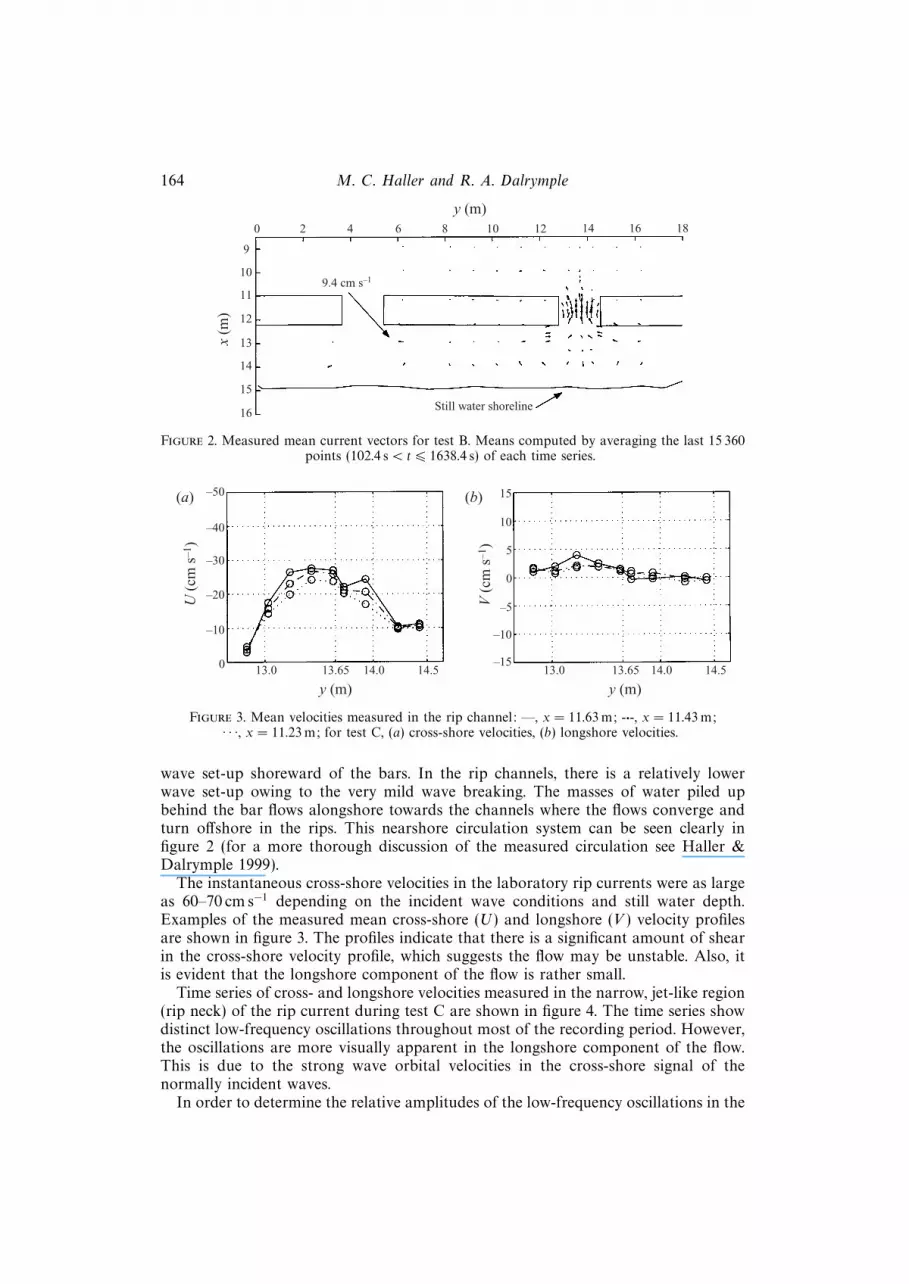
Figure 2. Measured mean current vectors for test B. Means computed by averaging the last 15 360points (102.4 s < t 6 1638.4 s) of each time series.

0

U (

cm s

–1)

y (m)

–10

–20

–30

–40

–50

13.0 13.65 14.0 14.5

(a)

y (m)13.0 13.65 14.0 14.5

(b)

0

–5

–10

–15

5

10

15V

(cm

s–1

)

Figure 3. Mean velocities measured in the rip channel: —, x = 11.63 m; -·-, x = 11.43 m;· · ·, x = 11.23 m; for test C, (a) cross-shore velocities, (b) longshore velocities.

wave set-up shoreward of the bars. In the rip channels, there is a relatively lowerwave set-up owing to the very mild wave breaking. The masses of water piled upbehind the bar flows alongshore towards the channels where the flows converge andturn offshore in the rips. This nearshore circulation system can be seen clearly infigure 2 (for a more thorough discussion of the measured circulation see Haller &Dalrymple 1999).

The instantaneous cross-shore velocities in the laboratory rip currents were as largeas 60–70 cm s−1 depending on the incident wave conditions and still water depth.Examples of the measured mean cross-shore (U) and longshore (V ) velocity profilesare shown in figure 3. The profiles indicate that there is a significant amount of shearin the cross-shore velocity profile, which suggests the flow may be unstable. Also, itis evident that the longshore component of the flow is rather small.

Time series of cross- and longshore velocities measured in the narrow, jet-like region(rip neck) of the rip current during test C are shown in figure 4. The time series showdistinct low-frequency oscillations throughout most of the recording period. However,the oscillations are more visually apparent in the longshore component of the flow.This is due to the strong wave orbital velocities in the cross-shore signal of thenormally incident waves.

In order to determine the relative amplitudes of the low-frequency oscillations in the

Rip current instabilities 165u

(cm

s–1

)

(a)6040200

–20– 40–60

v (c

m s

–1)

(b)3020

0–10–20–30

10

u (c

m s

–1)

6040200

–20– 40–60

u (c

m s

–1)

6040200

–20– 40–60

v (c

m s

–1)

3020

0–10–20–30

10

v (c

m s

–1)

3020

0–10–20–30

10

Time (s)0 200 400 600 800 1000 1200 1400 1600 0 200 400 600 800 1000 1200 1400 1600

Time (s)

c16 x = 11.23m, y = 13.63m; um = –23.7173 (cm s–1) c16 x = 11.23m, y = 13.63m; vm = 1.1198 (cm s–1)

c16 x = 11.43m, y = 13.63m; um = –25.8919 (cm s–1) c16 x = 11.43m, y = 13.63m; vm = 1.4154 (cm s–1)

c16 x = 11.63m, y = 13.63m; um = –27.0029 (cm s–1) c16 x = 11.63m, y = 13.63m; vm = 1.5064 (cm s–1)

Figure 4. Time series of (a) cross-shore velocity (u), (b) longshore velocity (v) measured near thecentre of the rip channel (test C, run 16; x = 11.23, 11.43, 11.63 m; y = 13.63 m).

Test B C D E G

σu 3.7 7.0 7.5 6.0 6.2σv 8.5 4.9 3.4 5.6 5.1Umax −19.7 −27.6 −40.8 −21.6 −21.8x 11.94 11.63 11.43 11.93 11.93y 13.53 13.43 14.24 14.24 13.63

Table 2. Table of standard deviations of lowpass filtered cross-shore, σu, and longshore, σv , velocities(cm s−1) measured in the rip neck. Umax is the maximum mean offshore current (cm s−1), x, y are themeasuring locations (m).

rip neck, the velocity data from each test were lowpass filtered (0 < f < 0.033 Hz) toremove the incident wave signal and any motions due to basin seiching (see AppendixA for seiching analysis). The standard deviations (σu, σv) of the filtered records areshown in table 2 along with the mean of the unfiltered cross-shore velocity record.The particular data record chosen for each test corresponds to the record from thelocation of the maximum measured mean offshore rip velocity. It is apparent fromthis data that σu and σv are of comparable amplitude and are a significant percentageof the mean velocity. The data indicate some variability in the magnitudes of σu andσv . This is mostly due to variability in the location of the measured maximum (Umax).Additional variability is likely owing to variability in the mean rip current direction,which was not always directly offshore. However, the variabilty of the total low-frequency current vector (σ|u|) at the rip maximum was much smaller (±1.3 cm s−1).

166 M. C. Haller and R. A. Dalrymple

9

10

11

12

13

14

10 12 14 16 18

9

10

11

12

13

14

10 12 14 16 18y (m)y (m)

x (m

)

x (m

)

(a) (b)

Figure 5. Contours of low-frequency (f 6 0.033 Hz) variance for test B, (a) cross-shore variance(σ2u), maximum contour 74.1 cm2 s−2 (b) longshore variance (σ2

v ), maximum contour 82.3 cm2 s−2.Contour interval is 8.23 cm2 s−2.

0 0.0075 0.02 0.03 0.04 0.05 0.02 0.03 0.04 0.050.0050

105

104

103

102

101

105

104

103

102

101

(a) (b)

95% confidence95% confidence95% confidence

95% confidence95% confidence95% confidence

Frequency (Hz)

Spe

ctra

l den

sity

(cm

2 s–1

)

Spe

ctra

l den

sity

(cm

2 s–1

)

Frequency (Hz)

Figure 6. Average energy spectrum of (a) cross-shore velocities and (b) longshore velocities measurednear the rip neck (test B, run 33; 275.2 s < t < 2732.7 s; x = 11.44 m, 11.74 m, 11.94 m; y = 13.53 m),∆f = 0.0012, d.o.f . = 18.

It is also important to note that these low-frequency current oscillations are localizednear the neck. Figure 5 shows the distribution of low-frequency variance (σ2

u , σ2v )

throughout the circulation system measured during test B. The contours clearly showa concentration of both u and v variance along the rip axis, especially in the gapbetween the bars. Since the variance is localized in the location of the rip neck andthe frequencies of the motions are much lower than predicted seiching modes (seeAppendix A), it is unlikely that basin resonances are a source for these motions.The contours shown in figure 5 also show that the low-frequency variances are muchsmaller at the basin centre (y = 9.1 m) and decay towards zero near the sidewall(y = 18.2 m). This suggests that the two rip currents were behaving independentlyand that the influence of the basin sidewalls on the low-frequency motions should belimited.

Spectral analysis of the velocity records measured along the rip current axis allowsus to estimate the specific timescales of these oscillations. Since these motions havesuch long timescales, the longer time series were used when available. The cross- andlongshore velocity spectra from each test along with the 95% confidence intervals anddegrees of freedom (d.o.f.) are shown in figures 6–10. Figure 6(b) suggests a dominant

Rip current instabilities 167

0 0.01 0.018 0.03 0.04 0.05 0.018 0.03 0.04 0.050.01

104

103

102

101

104

103

102

(a) (b)

95% confidence95% confidence95% confidence95% confidence95% confidence95% confidence

Frequency (Hz)

Spe

ctra

l den

sity

(cm

2 s–1

)

Spe

ctra

l den

sity

(cm

2 s–1

)

Frequency (Hz)

Figure 7. Averaged energy spectra of (a) cross-shore velocities and (b) longshore velocities fromextra long time series measured at x = 11.43 m, 11.63 m, 11.94 m, y = 13.63 m (test C, run 34;0 s < t < 6553.6 s), ∆f = 0.0012 Hz, d.o.f . = 48.

0.0183 0.033 0.0430.0049

104

103

102

101

104

103

102

(a) (b)

95% confidence95% confidence95% confidence95% confidence95% confidence95% confidence

Frequency (Hz)

Spe

ctra

l den

sity

(cm

2 s–1

)

Spe

ctra

l den

sity

(cm

2 s–1

)

Frequency (Hz)0.0183 0.033 0.0430.0049

101

Figure 8. Averaged energy spectra of (a) cross-shore velocities and (b) longshore velocitiesmeasured at x = 11.43 m, 11.63 m, 11.93 m, y = 13.03 m, 13.63 m, 14.24 m (test D, runs D1–3;819.2 s < t < 1638.4 s), ∆f = 0.0012 Hz, d.o.f . = 18.

0.03 0.04 0.050.02

104

103

102

101

104

103

102

(a) (b)

95% confidence95% confidence95% confidence95% confidence95% confidence95% confidence

Frequency (Hz)

Spe

ctra

l den

sity

(cm

2 s–1

)

Spe

ctra

l den

sity

(cm

2 s–1

)

Frequency (Hz)0.02 0.03 0.040.0098

101

0.00980.05

Figure 9. Averaged energy spectra of (a) cross-shore velocities and (b) longshore velocitiesmeasured at x = 11.43 m, 11.63 m, 11.93 m, y = 13.03 m, 13.63 m, 14.24 m (test E, runs E1–3;819.2 s < t < 1638.4 s), ∆f = 0.0012 Hz, d.o.f . = 18.

168 M. C. Haller and R. A. Dalrymple

0.039 0.050.026

104

103

102

101

104

103

102

(a) (b)

95% confidence95% confidence95% confidence95% confidence95% confidence95% confidence

Frequency (Hz)

Spe

ctra

l den

sity

(cm

2 s–1

)

Spe

ctra

l den

sity

(cm

2 s–1

)

Frequency (Hz)0.026 0.0390.013

101

0.0130.05

Figure 10. Averaged energy spectra of (a) cross-shore velocities and (b) longshore velocitiesmeasured at x = 11.43 m, 11.63 m, 11.93 m, y = 13.03 m, 13.63 m, 14.24 m (test G, runs G1–3;819.2 s < t < 1638.4 s), ∆f = 0.0012 Hz, d.o.f . = 18.

low-frequency mode of approximately 0.005 Hz for this test, which is an unusuallylarge timescale for laboratory scale systems.

Figure 7 shows the spectra from test C, which has the most degrees of freedomowing to its long length. The spectra clearly show energy peaks near 0.018 Hz in boththe cross-shore and longshore velocities. The spectra also indicate a lower-frequencypeak near 0.01 Hz. The v spectrum also shows higher-frequency peaks near 0.028and 0.036 Hz. The presence of these peaks suggests that the motions at the two low-frequency peaks are interacting nonlinearly, since the higher-frequency peaks centredat 0.028 Hz and 0.036 Hz are a sum frequency (0.01 + 0.018 Hz) and a harmonic(0.018 + 0.018 Hz).

The averaged rip current spectra for tests D, E, and G (figures 8–10) use the datafrom the three runs during each test when the ADVs were in the rip channel (1 runcontains 3 records), and therefore include more spatial averaging. Figure 8 and, to alesser extent, figure 10 again suggest that specific modes are interacting nonlinearly.Figure 8(b) shows numerous distinct peaks in the longshore velocity spectrum, whilein the cross-shore spectrum the peaks are less distinct. The dominant longshorevelocity peaks are at f1 = 0.0049 Hz, f2 = 0.0183 Hz, and f3 = 0.033 Hz. Here, again,there appear to be interaction peaks at 0.013 Hz (f2 − f1) and 0.023 Hz (f2 + f1).However, it is difficult to determine more definitively whether these low-frequencypeaks are interacting nonlinearly. The multiple peaks might also indicate the presenceof multiple independent linear modes.

Test E had similar wave height and rip current strength to test B. Likewise, thespectra from test E (figure 9) do not show numerous energetic peaks above 0.01 Hz.Instead, test E shows very low-frequency peaks near 0.005 Hz and 0.01 Hz in bothcross-shore and longshore velocity spectra. The spectral peaks for test G (figure 10)appear somewhat less distinct than those in tests C and D, however, the presence ofenergies near 0.013, 0.026, and 0.039 Hz again suggest that harmonics are present.

In order to gain an estimate of the lengthscales of the disturbances measured duringthe experiments, cross-spectra of longshore velocities were computed from runs whenthe ADVs were positioned in a cross-shore array located in the rip channel. Since therewere only three ADVs in operation during the experiments, and therefore only threesensor lags to compute cross-spectra, it was difficult to obtain statistically meaningful

Rip current instabilities 169

150

100

50

(a) (b)

Coh

eren

ce o

f v

Cross-shore lag (m)

0

–0.5

L = 2.73, C = –0.049, frequency = 0.018

1.0

0.8

0.6

0.4

0.2

0–0.4 –0.3 –0.2 –0.1 0

Cross-shore lag (m)–0.5 –0.4 –0.3 –0.2 –0.1 0

Pha

se o

f v

(deg

.)

Frequency = 0.018

Figure 11. (a) Phase vs. cross-shore sensor separation, (b) coherence vs. cross-shore sensor separationfor test C, run 34, ∆f = 0.0012 Hz, d.o.f . = 16. Solid line indicates 95% confidence level. Phasespeed (C) defined as L× freq , negative values indicate offshore propagation.

150

100

50

(a) (b)

Cross-shore lag (m)

0–0.5

L = 1.99, C = 0.024, frequency = 0.012

1.0

0.8

0.6

0.4

0.2

0–0.4 –0.3 –0.2 –0.1 0

Cross-shore lag (m)–0.5 –0.4 –0.3 –0.2 –0.1 0

Frequency = 0.01

Coh

eren

ce o

f v

Pha

se o

f v

(deg

.)

Figure 12. (a) Phase vs. cross-shore sensor separation, (b) coherence vs. cross-shore sensor separationfor test G, run 3, ∆f = 0.0024 Hz, d.o.f . = 8. Solid line indicates 95% confidence level. Phase speed(C) defined as L× freq , negative values indicate offshore propagation.

estimates of the disturbance wavelengths. However, figures 11 and 12 show the phaseand coherence as a function of cross-shore lag for two frequency bins during tests Cand G. Using the average phase variation as a function of distance, we can estimatethe wavelength (L) of the coherent motions at these frequencies. The experimentalestimates of the disturbance lengthscales are shown to be L = 2.7 m at f = 0.018 Hztest C, and L = 2 m at f = 0.012 Hz test G. These scales will be shown to comparefavourably with the model results given in § 3.

3. Rip current modellingIn this section we will concentrate on the modelling of a rip current in isolation.

The results shown in § 2.2 indicate that we may neglect the effects of the sidewallsand of rip current coupling. Therefore, we will consider a single rip current initializedat one boundary of a semi-infinite horizontal domain with a finite water depth.

170 M. C. Haller and R. A. Dalrymple

3.1. Governing equations

In order to model the rip current, we begin with the wave- and depth-averagedequations of motion (after Mei 1989),

u∗t + u∗u∗x + v∗u∗y = −gη∗x + R∗x + M∗x + T∗x, (3.1)

v∗t + u∗v∗x + v∗v∗y = −gη∗y + R∗y + M∗y + T∗y, (3.2)

(u∗h∗)x + (v∗h∗)y = −η∗t , (3.3)

where u∗, v∗, η∗, and h∗ represent the dimensional cross-shore and longshore velocity,water suface elevation, and total water depth (including set-down/set-up), respectively,and the subscripts indicate derivatives in x, y, and t. For the modelling section wewill adopt a coordinate system such that the x-axis is located along the centreline ofthe rip current and increasing in the offshore direction. The forcing due to radiationstress gradients, R∗x and R∗y (where the subscripts indicate the direction in which they

act; same for M∗x, M

∗y , T∗x, and T∗y), are defined dimensionally as

R∗x = − 1

ρh

(∂

∂xS∗xx +

∂

∂yS∗yx

), (3.4a)

R∗y = − 1

ρh

(∂

∂xS∗xy +

∂

∂yS∗yy

), (3.4b)

where S ∗i,j are the components of the radiation stress tensor and ρ is the fluid density.

The turbulent mixing terms, M∗x,y , are defined dimensionally as

M∗x = − 1

ρh

(∂

∂xF∗xx +

∂

∂yF∗yx

), (3.5a)

M∗y = − 1

ρh

(∂

∂xF∗xy +

∂

∂yF∗yy

), (3.5b)

where F∗i,j are the components of the Reynolds stress tensor. Finally, T∗x and T∗yrepresent the bottom friction components.

We seek to model the development of the rip from an initial starting point. In thisrespect, we are not modelling the forcing of the rip directly, but instead we will treat therip as an ambient free jet flow. In order to derive an analytical solution we will makecertain simplifications. We will adopt the classical ‘rigid-lid’ approximation, η∗t ≈ 0,and also assume a longshore uniform coast (h∗ = h∗(x)). The first approximation iscommonly used in the study of nearshore vorticity motions (see Falques & Iranzo1994 for a discussion), and the second is a reasonable starting point for the analysisof rip current dynamics and is not strictly violated within the rip current while itremains in the rip channel. This is essentially equivalent to assuming η∗y = 0.

We will also negelect the effects of wave–current interaction, such as wave refractiondue to the opposing current, following Tam (1973). Instead, we will assume that inthe x-direction the radiation stress forcing is balanced by the water surface gradientsuch that

gη∗x = R∗x, (3.6)

and we will neglect the radiation stress forcing in the y-direction, R∗y . While it iscertain that the rip current modifies the wave heights and the wave breaking in the

Rip current instabilities 171

channel, the results of Yoon & Liu (1990) suggest that we may neglect the effects ofradiation stress gradients on the evolution of the jet. Their numerical study indicatesthat the dominant processes driving jet spreading are bottom friction and turbulentmixing. Our purpose here is to obtain a reasonably simplified analytical solution forthe rip current flow that contains the dominant physical mechanisms governing therip dynamics, and, even more importantly, compares favourably with the measuredmean data so that we can analyse the stability characteristics of the flow.

Using the above assumptions we cross-differentiate (3.1) and (3.2) and combinewith (3.3) to obtain the dimensional, vorticity transport equation for a longshoreuniform coast,

D

Dt

(u∗y − v∗xh∗

)= − 1

h∗∇h × (M ∗ + T∗), (3.7)

where the horizontal gradient operator is defined such that ∇h × M ∗ = ∂M∗y/∂x −

∂M∗x/∂y. In order to non-dimensionalize the above equation, we introduce the basic

scales

u∗, v∗ ∼ U0, h∗ ∼ h0, M ∗ ∼ U20/b0,

x, y ∼ b0, t ∼ b0/U0, T∗ ∼ U20/h0,

where U0 is a velocity scale, b0 is a horizontal lengthscale, and h0 is a depth scale.Substitution of the scales leads us to the following non-dimensional vorticity transportequation:

D

Dt

(uy − vxh

)= −1

h∇h × M +

b0

h0

(−1

h∇h × T

), (3.8)

(x, y, t are now also non-dimensional). We next assume our basic state is a steadymean flow with superimposed small disturbances such that

u(x, y, t) = U(x, y) + u(x, y, t), (3.9a)

v(x, y, t) = V (x, y) + v(x, y, t), (3.9b)

M (x, y, t) = M 0(x, y) + ∆M (x, y, t), (3.9c)

T(x, y, t) =T0(x, y) + ∆T(x, y, t), (3.9d)

where U,V represent the steady mean flow, u, v are the disturbance velocities, andM 0 and T0 represent the turbulent mixing and bottom stress in the absence ofdisturbances.

Equation (3.8), in the absence of disturbances (i.e. u = v = 0), can now be writtenas

U

(Uy − Vx

h

)x

+ V

(Uy − Vx

h

)y

= −1

h∇h ×M 0 +

b0

h0

(−1

h∇h ×T0

), (3.10)

where h = h (non-dimensional water depth). This is the governing non-dimensionalvorticity transport equation for steady flow.

Subtracting (3.10) from (3.8) and linearizing in the disturbance velocities, we obtain(∂

∂t+U

∂

∂x+ V

∂

∂y

)(uy − vxh

)+

(u∂

∂x+ v

∂

∂y

)(Uy − Vx

h

)=

− 1

h∇h × ∆M +

b0

h0

[−1

h∇h × ∆T

], (3.11)

172 M. C. Haller and R. A. Dalrymple

which represents the governing non-dimensional vorticity transport equation for thedisturbed flow. Next, we will examine solutions to these equations by first specifyingthe form of the steady flow and then searching for growing solutions (instabilities) tothe disturbance equation.

3.2. Time-averaged flow

Previous researchers have used simplified forms of (3.10) to model the mean flowsin rip currents. For example, Arthur (1950) developed an analytical model thatsatisfied the inviscid form of (3.10) and matched the general characteristics of a ripcurrent quite well. His model produced a long and narrow rip, supplied by nearshorefeeder currents, which decayed in magnitude and spread laterally as it extendedoffshore. However, the rate of rip current spreading was essentially arbitrary and givenwithout justification, and viscous effects were not considered. Tam (1973) determineda similarity solution to the rip current flow in a transformed coordinate system basedon a boundary-layer analogy and investigated the influence of the bottom slope onthe steady flow in the absence of bottom friction. His solution is mathematicallyequivalent to the Bickley jet (Bickley 1939). We will use a similar approach here;however, our approach is simpler as our coordinate system is more straightforward.We will also include the effects of bottom friction and compare to measured data.Our approach to the steady-flow problem will most resemble the approach of Joshi(1982), who analysed the hydromechanics of tidal jets. In contrast to Joshi (1982), wewill approach the problem more generally in terms of a non-dimensional nearshorevorticity balance and apply the method of multiple scales, and also, we will presenta simplified relationship for determining the empirical mixing and bottom frictioncoefficients from the experimental data.

The main purpose of this section is to develop a tractable model for the mean flowsin a rip current so that we can investigate the stability characteristics of rip currents.Since the tidal jet model of Joshi contains the dominant mechanisms (turbulentmixing, bottom friction, variable bathymetry) governing the evolution of shallowwater jets, we shall follow it closely. However, because the scales of tidal jets andrip currents are quite different, it will be important to test how well the modelledmean flows compare with the experimental data in order to verify the validity of themodel for rip currents. We will also describe how the effects of turbulent mixing andbottom friction affect the rate of rip current spreading and the decay of rip velocitiesin the offshore direction so that we can subsequently interpret the results from therip current instability model.

We will restrict our analysis of (3.10) to flows that are slightly non-parallel suchthat they are slowly varying in the cross-shore direction. Therefore, we introduce ascaled cross-shore coordinate x1 such that

x1 = εx, (3.12)

where ε is a small dimensionless parameter that represents the slow variation of theflow. Thus, the steady-flow components are given by

U = U(x1, y), (3.13a)

V = εV (x1, y), (3.13b)

h = h(x1), (3.13c)

where (3.13b) indicates that the transverse velocity (V (x, y)) is finite but small beforethe coordinate transformation (i.e. slightly non-parallel flow). After substituting the

Rip current instabilities 173

scaled coordinate, the left-hand side of (3.10) becomes

εU

(Uy − ε2Vx1

h

)x1

+ εV

(Uy − ε2Vx1

h

)y

= R.H.S. (3.14)

Next, we must parameterize the turbulent mixing and bottom friction terms. Itis common to neglect the normal Reynolds stress terms (F∗xx, F∗yy) since they aregenerally small. We shall parameterize the remaining terms using Prandtl’s ‘apparentkinematic viscosity’ hypothesis with a turbulent eddy viscosity, νT , such that thenon-dimensional turbulent mixing terms take the following forms

Mx =1

h

∂

∂y(h νT uy), (3.15a)

My =1

h

∂

∂x(h νT uy). (3.15b)

After introducing the scaled coordinate, the mixing in the absence of disturbancestakes the forms

M0x1

=1

R t

∂

∂y(Um`Uy), (3.16a)

M0y =

ε

R t

1

h

∂

∂x1

(hUm`Uy), (3.16b)

where Rt is a constant non-dimensional turbulent Reynolds number defined as Rt ≡Um`/νT , ` is a mixing length, and Um represents the velocity at the rip currentcentreline and varies in the cross-shore direction. For the bottom friction, we will usethe following nonlinear formulations

Tx = − fd8hu |u|, (3.17a)

Ty = − fd8hv |u|, (3.17b)

where fd is a Darcy–Weisbach friction factor and u is the total current vector. In theabsence of disturbances, the scaled variables for the bottom friction terms become

T0x1

= − fd8 hU(U2 + ε2 V 2)1/2, (3.18a)

T0y1

= −εfd8 h

V (U2 + ε2V 2)1/2. (3.18b)

It is evident, since the terms in (3.14) are O(ε) or smaller, that the parameter 1/Rt in(3.16) must be at least as large as O(ε) in order to retain the effects of turbulent mixingon the time-averaged flow. Therefore, we will retain M0

x1and neglect the smaller term

M0y1

. Likewise, we take the non-dimensional frictional parameter ft ≡ fdb0/8h0 to

be O(ε), and therefore retain T0x1

and neglect T0y1

. The governing equation for thetime-averaged rip current flow can then be written as

UUyx1−UUy

hx1

h+ VUyy =

1

Rt

(Um`Uyyy

)− ft(2UUy

h

). (3.19)

We will treat the rip current as a self-preserving turbulent jet. The self-preservation

174 M. C. Haller and R. A. Dalrymple

of the jet implies that the evolution of the flow is governed by local scales of lengthand velocity (Tennekes & Lumley 1972). We will take the local lengthscale to be` = b(x1), the half-width of the jet, and the velocity scale, Um(x1), to be the localvelocity at the jet centreline. In addition, if the jet is self-preserving, the dimensionlessvelocity profiles U/Um at all x1 locations will be identical when plotted against thedimensionless coordinate y/b. Therefore, we introduce a similarity variable

η =y

b(x1), (3.20)

and we assume thatU(x1, y)

Um(x1)= f(η) only. (3.21)

It is important to note here that y was previously non-dimensionalized by theconstant b0, which we have defined as the jet width at the origin. The jet widthb(x1) has also been non-dimensionalized by b0, and therefore b(0) = 1. Similarly,the velocities have been non-dimensionalized by U0 which we have defined as themaximum velocity at the origin, therefore Um(0) = 1.

In order to write (3.19) in terms of similarity variables, we must first obtain anexpression for V (x1, η). We do this by integrating the non-dimensional form of (3.3)from 0 to y at a given x1, using the condition of zero transverse flow at the jetcentreline (V (x1, η = 0) = 0), to obtain

V = Umbx1ηf −

(Umx1

b+Um

hx1

hb+Umbx1

)∫ η

0

f dη′. (3.22)

For the mixing term we will assume self-preservation of the Reynolds stress such thatwe can express the mixing as

1

RtUm `Uy = U2

m g(η), (3.23)

where g(η) is an as yet unspecified similarity function.Substitution of the similarity forms of the velocities and Reynolds stress into (3.19)

and simplifying, leads us to the following(bUmx1

Um

− bx1− b hx1

h+ 2

ft b

h

)ffη −

(bUmx1

Um

+b hx1

h+ bx1

)fηη

∫ η

0

fdη′ = gηη,

(3.24)where subscripts η and x1 represent derivatives. Note that f and g do not dependexplicitly on x1, whereas the coefficients on the left-hand side of (3.24) are generallyfunctions of x1. Therefore, for this equation to hold throughout the region of study,the coefficients must be independent of x1. If we alternately add and subtract these tworelations (the expressions in parentheses in (3.24)), we obtain the following equationsgoverning the length and velocity scales

bx1+

(hx1

h− ft

h

)b = C, (3.25)

Umx1+

(ft

h− C1

b

)Um = 0, (3.26)

where C and C1 are true constants. These equations can be solved by the method ofvariation of parameters (see e.g. Greenberg 1988 pp. 907–909) to obtain the following

Rip current instabilities 175

10

5

0

(a) (b)

–10

0.8

x1

0 1 2 3 4 5

–5

b(x

1)

x1

0 1 2 3 4 5

1.0

0.6

0.4

0.2

Um

Figure 13. Cross-shore variation of the rip current scales (a) jet width vs. cross-shore distance (b)centreline velocity vs. cross-shore distance for —, classical plane jet, - - -, flat bottom w/friction(ft = 1), · · · , planar beach (m1 = 1, ft = 0), -·-, frictional planar beach (m1 = ft = 1) (dash-dot ison top of solid line in (a).

general solutions for the width and velocity scales of the jet

b(x1) =1

h(x1)exp

(ft

∫ x1

0

h−1dξ

)[1 + C

∫ x1

0

h(ξ1) exp

(−ft

∫ ξ1

0

h−1dζ

)dξ1

],

(3.27)

Um(x1) = C3 exp

(−ft

∫ x1

0

h−1 dξ

)[1 + C

∫ x1

0

h(ξ1) exp

(−ft

∫ ξ1

0

h−1 dζ

)dξ1

]C1/C

,

(3.28)

where the lower limit of integration has been chosen to be x1 = 0, also the non-dimensional depth at the origin has been specified as h(0) = 1; thus, C,C1, and C3 arethe three constants we are left to evaluate. The relationships between the constants(C,C1, C3, Rt) and the functional form of f are given in Appendix B.

For a frictionless flat bottom, (3.27) and (3.28) collapse to the classical plane jetsolution whereby the width scale grows linearly along the jet axis and the centrelinevelocity decays with x−1/2. Figure 13 shows the variation of the width scale and thecentreline velocity in the offshore direction for specific parameter values. It can beseen that friction increases the jet spreading and causes the centreline velocity todecay more rapidly. In contrast, the jet spreading is reduced by an increasing depthin the offshore direction owing to vortex stretching (Arthur 1962). In addition, if thefrictional spreading effects are balanced by the narrowing due to vortex stretching(ft = m1), then the jet spreads linearly at the same rate as the classical plane jet. Theseresults are equivalent to those described by Joshi (1982) for the tidal jet.

3.2.1. Comparison to data

Next, we compare the results from our model for rip current mean flows withthe measured velocity profiles from the experiments. For the comparison, we adopta new cross-shore coordinate axis x′ = x0 − x where x0 is the cross-shore location(dimensional) of the base of the rip current during the experiments. Thus, x′ is nowincreasing in the offshore direction and the location of the jet origin, x0, is determinedas the experimental location where the rip begins to exhibit decay of its centrelinevelocity and is different for each test. The location of the rip current centreline, y0, is

176 M. C. Haller and R. A. Dalrymple0.5(a) (b)

–1.0

y–y0 (m)

01.0

–U(m

s–1

)

0.4

0.3

0.2

0.1

–0.5 0 0.5

0.5

–1.0

y–y0 (m)

01.0

–U(m

s–1

)

0.4

0.3

0.2

0.1

–0.5 0 0.5

(c) 0.5

–1.0

y–y0 (m)

01.0

–U(m

s–1

)

0.4

0.3

0.2

0.1

–0.5 0 0.5

Figure 14. Comparison of best fit mean rip current velocity profile to experimental data for test B(a) x′ = 0 m (x = 11.94 m), (b) x′ = 0.2 m (x = 11.74 m), (c) x′ = 0.5 m (x = 11.44 m).

determined by taking a weighted average of the mean rip current velocities measuredat the jet origin. This is given by

y0 =

N∑i=1

U(i)y(i)∆y(i)

N∑i=1

U(i)∆y(i)

, (3.29)

where N is the number of observations made at the jet origin.Once x0 and y0 were determined, the choices of the dimensional velocity and width

scales, U0 and b0, respectively, were made by a fitting procedure performed usingthe rip velocity profile at the origin. The statistical parameter we use to determinethe best fit of the modelled velocity profile to the experimental data is the index ofagreement di that was proposed by Wilmott (1981) and is given by

di = 1−

N∑i=1

(β(i)− α(i))2

N∑i=1

(|β(i)− α|+ |α(i)− α|)2

, (3.30)

where α(i) and β(i) are the measured and model data, respectively, and α is themeasured data mean. This parameter varies between 0 and 1 with di = 1 representingcomplete agreement. The scales U0 and b0 were then determined by a search procedure

Rip current instabilities 1770.5(a) (b)

–1.0

y–y0 (m)

01.0

–U(m

s–1

)

0.4

0.3

0.2

0.1

–0.5 0 0.5

0.5

–1.0

y–y0 (m)

01.0

–U(m

s–1

)

0.4

0.3

0.2

0.1

–0.5 0 0.5

(c) 0.5

–1.0

y–y0 (m)

01.0

–U(m

s–1

)

0.4

0.3

0.2

0.1

–0.5 0 0.5

Figure 15. Comparison of best fit mean rip current velocity profile to experimental data for test C(a) x′ = 0 m (x = 11.63 m), (b) x′ = 0.2 m (x = 11.43 m), and (c) x′ = 0.4 m (x = 11.23 m).

Test x0 (m) y0 (m) U0 (cm s−1) b0 (cm) di Rt ft d′iB 11.94 13.68 19.7 73 0.96 4.25 0.48 0.88C 11.63 13.57 29.1 64 0.94 4.75 0.48 0.90D 11.43 13.74 49.0 62 0.91 — — —E 11.93 13.8 28.4 52 0.94 2.5 0.46 0.94G 11.93 13.68 23.4 71 0.95 2.75 0.44 0.97

Table 3. Table of rip current scales determined by parameter search procedure, x0 cross-shorelocation of rip current origin, y0 longshore location of rip current centreline, U0 velocity scale, b0

width scale, di index of agreement for velocity profile at origin, Rt turbulent Reynolds number, ftbottom friction parameter, d′i index of agreement velocity along rip centreline.

where the index of agreement was computed for a large range of possible scales(∆U0 = 0.1 cm s−1, ∆b0 = 1 cm) and the best fit was chosen from the maximum valueof di.

The mixing and friction scales Rt and ft were also determined by a similar pro-cedure. It is evident from (B 5) and (B 10) that the decay of the centreline velocityis directly related to the values of Rt and ft. Therefore, these parameters were de-termined by fitting the decay of the centreline velocity between the model and datausing a parameter search with a resolution of ∆Rt = 0.25 and ∆ft = 0.0093. Sincethe experimental data points were never located at the exact centreline of the ripthe model/data comparison was made with the data points located closest to thecentreline.

178 M. C. Haller and R. A. Dalrymple

0.5

–1.0

y–y0 (m)

01.0

–U(m

s–1

)

0.4

0.3

0.2

0.1

–0.5 0 0.5

Figure 16. Comparison of best fit mean rip current velocity profile to experimental data for testD, x′ = 0 m (x = 11.43 m).

0.5(a) (b)

–1.0y–y0 (m)

01.0

–U(m

s–1

)

0.4

0.3

0.2

0.1

–0.5 0 0.5

0.5

–1.0y–y0 (m)

01.0

–U(m

s–1

)

0.4

0.3

0.2

0.1

–0.5 0 0.5

(c) 0.5

–1.0

y–y0 (m)

01.0

–U(m

s–1

)

0.4

0.3

0.2

0.1

–0.5 0 0.5

Figure 17. Comparison of best-fit mean rip current velocity profile to experimental data for test E(a) x′ = 0 m (x = 11.93 m), (b) x′ = 0.3 m (x = 11.63 m), (c) x′ = 0.5 m (x = 11.43 m).

The best-fit modelled velocity profiles are shown in figures 14–18. The dimensionalscales and the index of agreement for each test are listed in table 3. No estimateof Rt and ft could be made for test D since the decay of the rip current velocityis not captured by the measurements. The best-fit values for the friction factor fd(fd = 8fth0/b0) are at least an order of magnitude higher than those normally foundon field beaches, however, they compare well with those used in the modelling oflongshore currents in the laboratory (Kobayashi, Karjadi & Johnson 1997). Also, thebest fit values of Rt are found to be significantly lower than those reported previously

Rip current instabilities 179

0.5(a) (b)

–1.0y–y0 (m)

01.0

–U(m

s–1

)

0.4

0.3

0.2

0.1

–0.5 0 0.5

0.5

–1.0y–y0 (m)

01.0

–U(m

s–1

)

0.4

0.3

0.2

0.1

–0.5 0 0.5

(c) 0.5

–1.0

y–y0 (m)

01.0

–U(m

s–1

)

0.4

0.3

0.2

0.1

–0.5 0 0.5

Figure 18. Comparison of best-fit mean rip current velocity profile to experimental data for test G(a) x′ = 0 m (x = 11.93 m), (b) x′ = 0.3 m (x = 11.63 m), (c) x′ = 0.5 m (x = 11.43 m).

for plane jets, which have suggested Rt ≈ 25. The present results indicate that therip current has a faster spreading rate than a traditional plane jet. This is probablya direct result of the increased importance of non-parallel effects (turbulent mixingand bottom friction) in rip current flows. An additional source of turbulent mixing,not directly considered here, is the presence of instabilities of finite amplitude. Thiswill be discussed further with regard to the linear stability model in § 3.3. Finally, thetabulated values of the index of agreement show that the model was reasonable infitting to the measured profiles, since the index of agreement is at least 0.88 for allcases. However, it should be noted that for many of the tests there were only threedata points for comparison, which is a very small number.

3.3. Linear stability analysis

Next, we derive a linear stability model for the viscous turbulent jet. Returning tothe governing equation for the disturbed flow (3.11) and substituting the mixingparameterization (3.16), we have the following expressions for the mixing in thepresence of disturbances:

∆Mx =1

Rt

∂

∂y(Um b uy), (3.31a)

∆My =1

hRt

∂

∂x(hUm b uy). (3.31b)

180 M. C. Haller and R. A. Dalrymple

Likewise, using the bottom friction parameterization (3.18) the bottom stress termsin the presence of disturbances become

∆Tx = − fd8 h

(U + u)|U + u|+ fd

8 hU|U |, (3.32a)

∆Ty = − fd8 h

(V + v)|U + u|+ fd

8 hV |U |, (3.32b)

where U and u are the steady and disturbance current vectors, respectively.Using (3.3) we can introduce a stream function ψ(x, y, t) for the disturbances, such

that

ψy = uh, (3.33a)

−ψx = vh. (3.33b)

We then consider a normal-mode analysis of (3.11) and assume a harmonic depen-dence on x and t, so the stream function takes the form

ψ(x, y, t) = φ(y) ei(kx−ωt), (3.34)

and the eigenfunction φ contains the transverse structure of the instabilities.At this point there are two ways to approach the instability eigenvalue problem.

The first approach is to seek unstable modes that grow in time from disturbances at agiven wavenumber. This temporal instability approach assumes that the wavenumber,k ≡ 2π/L, is real and the eigenvalue, ω, is in general complex with the real part, ωr ,being the angular frequency, and the imaginary part, ωi, being the temporal growthrate. From inspection of (3.34), it is evident that a given mode is linearly unstableif ωi > 0, since the mode will then grow in time. Of course, in practice, neglectednonlinear effects will restrict growth at some finite value.

The second approach seeks unstable modes that grow spatially with propagationdistance from an initial disturbance at a given frequency. Conversely, the spatialinstability approach assumes ω to be purely real and the eigenvalue k is, in general,complex with kr representing the wavenumber (2π/L) and ki the spatial growth rate.A given mode is linearly unstable when ki < 0 and will grow as it propagatesdownstream with the mean current U.

The spatial theory is a better representation of the physical experiments, since thedisturbances must be initiated locally at the upstream end of the current, and growdownstream. Also, the temporal theory assumes an initial disturbance that is uniformin the cross-shore direction and is, therefore, not valid here since the mean flow isspatially varying in the cross-shore direction. A discussion of the results of temporaljet instability theory as applied to the rip current problem can be found in Haller &Dalrymple (1999). In the following analysis, we will consider only spatially growinginstabilities.

In order to account for the non-parallel nature of the flow in the stability analysis,we will use the method of multiple scales in a similar fashion to Nayfeh, Saric &Mook (1974) who applied it to boundary-layer flows. Assuming ε to be small, weexpand the disturbance stream function ψ in the following form

ψ(x1, y, t) = [φ0(x1, y) + εφ1(x1, y)] eiθ, (3.35)

where∂θ

∂x= k0(x1),

∂θ

∂t= −ω, (3.36)

Rip current instabilities 181

with the real part of k0 being the non-dimensional wavenumber, the imaginary partbeing the growth rate and ω is the non-dimensional frequency.

In terms of x1 and θ, the spatial and temporal derivatives transform according to

∂

∂x= k0(x1)

∂

∂θ+ ε

∂

∂x1

, (3.37a)

∂

∂t= −ω ∂

∂θ, (3.37b)

therefore, the fast scale describes the axial variation of the travelling-wave disturbancesand the slow scale is used to describe the relatively slow variation of the wavenumber,growth rate, and disturbance amplitude.

Substituting the assumed stream function and the mixing and bottom stress pa-rameterizations into the governing equation we then separate the terms by order inε. The governing equation at order ε0 is given by(

U − ω

k

)(φ0yy − k2

0φ0)− φ0Uyy = 0, (3.38)

orL(φ0) = 0,

which is the Rayleigh stability equation. The non-parallel effects appear in the O(ε)equation which is given by

L(φ1) = d1φ0x1+ d2φ0x1yy

+ d3φ0y + d4φ03y+ d5φ0 + d6φ0yy + d7φ04y, (3.39)

and the coefficients are given in Appendix C.The eigenvalue problem defined by (3.38) (with U(x1, y) given by (3.19)) can be

solved numerically to determine the eigenvalue k0 for a given ω. In order to solvethe inhomogeneous second-order problem we must first determine kx1

and φ0x1. We

can derive an expression for φ0x1by differentiating (3.38) with respect to x1, and we

obtain after simplificationL(φ0x1

) = A1 + k0x1A2, (3.40)

where the coefficients are given by

A1 = (Uyyx1+ k2

0Ux1)φ0 −Ux1

φ0yy ,

A2 = (2k0U − ω)φ0 − ω

k20

φ0yy .

The inhomogeneous equation governing φ0x1has a solution if, and only if, the

inhomogeneous terms are orthogonal to every solution of the adjoint homogeneousproblem. This constraint is expressed as∫ ∞

−∞(A1 + k0x1

A2)φ∗0 dy = 0, (3.41)

where φ∗0 is the eigenfunction from the adjoint eigenproblem given by

(U − c)φ∗0yy + 2Uyφ∗0y− k2(U − c)φ∗0 = 0. (3.42)

Equation (3.41) can be rearranged to give the following expression for the derivativeof the wavenumber

k0x1= −

∫ ∞−∞A1 φ

∗0 dy∫ ∞

−∞A2 φ

∗0 dy

. (3.43)

182 M. C. Haller and R. A. Dalrymple

0.5(a) (b)

ωr

0 1.0

0.4

0.276

0.2

0.1

0.255 0.5

2.0

0 1.0

1.5

1.0

0.639

0.255 0.51.5

ki kr

1.5ωr

Figure 19. (a) Spatial growth rate vs. frequency and (b) wavenumber vs. frequency for the parallelturbulent jet. —, sinuous modes; - - -, varicose modes; all variables are non-dimensional.

Once k0x1is known, (3.40) can be integrated to obtain φ0x1

.Finally, the complex wavenumber including non-parallel effects is given (to order

ε) by

k ≡ (k0 + εk1), (3.44)

where k1 is given in Appendix C, and ki is now the local growth rate and kr thelocal wavenumber. The small parameter ε is the ratio between the longshore andcross-shore velocity scales or Vmax/Umax, which for the viscous, turbulent jet is

ε ≡ Vmax

Umax

=2

Rt. (3.45)

3.3.1. Model results

A reasonable first estimate of the instability scales of the rip current is givenby the zeroth-order stability equation (3.38), these results correspond to the resultsfrom a purely parallel flow theory. The solutions fall into two categories, sinuous orvaricose, depending on whether ψ is an even or odd function of y, respectively. Thespatial instability curve and dispersion relation (zeroth-order solution) for the ripcurrent disturbances are shown in figure 19 for both the sinuous and varicose modes.As a check on these results, the temporal stability curves were calculated from thespatial results using Gaster’s relations (Gaster 1962). The temporal results, calculatedin this manner, are in excellent agreement with the directly computed temporalresults of Drazin & Howard (1966) who studied the Bickley jet (U = sech2(y)). Thecorresponding flow vectors of the parallel jet including the instabilities (FGM) areshown in figure 20.

The spatial results, shown in figure 19, indicate that the sinuous modes havethe highest growth rates, and the fastest growing sinuous mode (FGM) has non-dimensional frequency ω = 0.255, wavenumber kr = 0.639, and phase speed (C =ω/kr) that is nearly 40% of the maximum jet velocity. It is interesting to note thatthere is a large difference between the scales of the spatial FGM and the temporalFGM (ωr = 0.46, k = 1.0). Therefore, unlike many other instabilities (e.g. longshorecurrent instabilities, see Dodd & Falques 1996) the temporal theory, in the rip currentcase, cannot be assumed to apply for spatially growing disturbances. However, thespatial results can be calculated accurately from the temporal results using Gaster’srelations at this level of approximation.

Rip current instabilities 183

5(a) (b)

y

0

4

3

2

1

–2 00

2

x1

y–2 0 2

1

2

3

4

5

6

x1

Figure 20. Flow vectors of the parallel turbulent jet including the instability (FGM) for (a) sinuousmode, (b) varicose mode, the amplitude of the instability is arbitrary and has been chosen such thatthe flow pattern is easily visualized.

0.5(a) (b)

ω0 1.0

0.4

0.3

0.2

0.1

0.255 0.5

2.0

0 1.0

2.5

1.0

1.5

0.255 0.51.5

ki kr

1.5ω

0.5

Figure 21. (a) Growth rate vs. frequency (b) wavenumber vs. frequency for different turbulentReynolds numbers, - - -, Rt = 5; · · · , Rt = 10; -·-, Rt = 25; —, parallel flow, all variables arenon-dimensional and results are for flat bottom and ft = x1=0 (sinuous mode only).

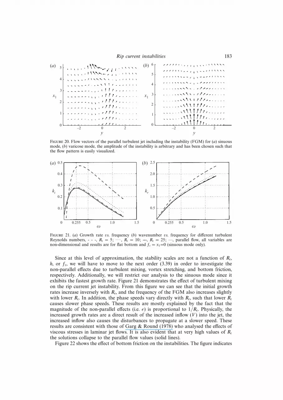
Since at this level of approximation, the stability scales are not a function of Rt,h, or ft, we will have to move to the next order (3.39) in order to investigate thenon-parallel effects due to turbulent mixing, vortex stretching, and bottom friction,respectively. Additionally, we will restrict our analysis to the sinuous mode since itexhibits the fastest growth rate. Figure 21 demonstrates the effect of turbulent mixingon the rip current jet instability. From this figure we can see that the initial growthrates increase inversely with Rt, and the frequency of the FGM also increases slightlywith lower Rt. In addition, the phase speeds vary directly with Rt, such that lower Rtcauses slower phase speeds. These results are mostly explained by the fact that themagnitude of the non-parallel effects (i.e. ε) is proportional to 1/Rt. Physically, theincreased growth rates are a direct result of the increased inflow (V ) into the jet, theincreased inflow also causes the disturbances to propagate at a slower speed. Theseresults are consistent with those of Garg & Round (1978) who analysed the effects ofviscous stresses in laminar jet flows. It is also evident that at very high values of Rtthe solutions collapse to the parallel flow values (solid lines).

Figure 22 shows the effect of bottom friction on the instabilities. The figure indicates

184 M. C. Haller and R. A. Dalrymple

0.5(a) (b)

ω0 1.0

0.4

0.3

0.2

0.1

0.255 0.5

2.0

0 1.0

2.5

1.0

1.5

0.255 0.51.5

kikr

1.5ω

0.5

3.0

Figure 22. (a) Growth rate vs. frequency, (b) wavenumber vs. frequency for different values ofbottom friction, - - -, ft = 0.01; · · · , ft = 0.2; -·-, ft = 0.4; —, parallel flow, all variables arenon-dimensional and results are for flat bottom, x1=0, and Rt = 5 (sinuous mode only).

0.5

(a) (b)

ω0 1.0

0.4

0.3

0.2

0.1

0.255 0.5

2.0

0 1.0

2.5

1.0

1.5

0.255 0.51.5

kikr

1.5ω

0.5

0.6

Figure 23. (a) Growth rate vs. frequency, (b) wavenumber vs. frequency for different bottomslopes, -·-·, m1 = 0.001; · · ·, m1 = 0.01; - - -, m1 = 0.1; —, parallel flow m1 = 0, all variables arenon-dimensional, ft = 0 and Rt = 5.

that increased bottom frictional dissipation causes an increase in the initial growthrates and a decrease in the range of unstable frequencies. The increased growth ratesare due to the effect of the decay of the centreline velocity. Essentially, since withincreased bottom friction the jet initially spreads very quickly, the inflow is initiallymuch stronger and therefore the jet is more unstable. Additionally, the increasedbottom friction causes the disturbances to propagate more slowly, as can be seen bythe dispersion curves. The results collapse to those for ft = 0 and Rt = 5 (figure 21)for very low friction.

Figure 23 shows the effects of different bottom slopes on the instabilities. The resultsindicate that increased bottom slope increases the growth rates at x1 = 0. This isrelated to the effects of vortex stretching and of spatial deceleration of the rip current.Though the jet does not spread as quickly on a sloping beach compared to a flatbottom owing to vortex stretching, the centreline velocity decays more quickly withincreased beach slope owing to continuity effects. This increased spatial decelerationcauses the growth rates to increase. Also, the phase speeds of the disturbances increaseon the relatively narrower jets of planar beaches.

Rip current instabilities 185

0.8

(a) (b)

ω0 0.4

0.6

0.4

0.2

0.1 0.25

2.0

0 0.2

1.0

1.5

0.10.5

k 0i, k

i

0.4

ω

0.5

1.0

0.3 0.5

k 0r, k

r

Figure 24. (a) Growth rate vs. frequency, (b) wavenumber vs. frequency for test B, all variables arenon-dimensional. —, x′ = 0 m; - - -, x′ = 0.2 m; · · · , x′ = 0.5 m, upper curves include non-paralleleffects (k), lower curves are for parallel flow theory (k0).

0.8

(a) (b)

ω0 0.3

0.6

0.4

0.2

0.1 0.2

2.0

0 0.2

1.0

1.5

0.10.5

k 0i, k

i

0.4ω

0.5

1.0

0.3 0.5

k 0r, k

r

0.4

Figure 25. (a) Growth rate vs. frequency, (b) wavenumber vs. frequency for test C, all variables arenon-dimensional. —, x′ = 0; - - -, x′ = 0.2 m; · · · , x′ = 0.4 m, upper curves include non-paralleleffects (k), lower curves are for parallel flow theory (k0).

3.3.2. Model/data comparison

With the rip scales listed in table 3, we can now use the stability model to investigatethe instability characteristics of the experimental rip currents. Figures 24–27 show thegrowth rates and dispersion relations for the sinuous modes of rip current instability atthree different locations along the jet axis. It is immediately evident from these figuresthat the non-parallel effects strongly affect the growth rates and phase speeds of thedisturbances and the growth rates decline as the jet spreads. In addition, the predicteddimensional timescales of the fastest growing modes compare well with the measuredspectra shown in § 2.2. The predicted dimensional scales of the FGM for each testare listed in table 4 along with the measured values of the nearest significant spectralpeak shown in figures 6, 7, and 8–10. It is evident that the predicted frequencies ofthe FGM do correspond with peaks in the measured spectra for tests C, D, andG. The predicted frequency agrees less well with that measured frequency in tests Band E.

Finally, it should be considered that the modelled mean velocity profiles used inthe instability analysis were fit to measured data that includes the effects of the finite

186 M. C. Haller and R. A. Dalrymple

1.5

(a) (b)

ω0 0.3

1.0

0.5

0.1 0.2

2.0

0 0.2

1.0

1.5

0.1

k 0i, k

i

ω

0.5

2.0

0.3

k 0r, k

r

Figure 26. (a) Growth rate vs. frequency, (b) wavenumber vs. frequency for test E, all variables arenon-dimensional. —, x′ = 0 m; - - -, x′ = 0.3 m; · · · , x′ = 0.5 m, upper curves include non-paralleleffects (k), lower curves are for parallel flow theory (k0).

1.5(a) (b)

ω

0 0.3

1.0

0.5

0.1 0.2

2.0

0 0.2

1.0

1.5

0.1

k 0i, k

i

ω

0.5

0.3

k 0r,

kr

Figure 27. (a) Growth rate vs. frequency, (b) wavenumber vs. frequency for test G, all variables arenon-dimensional. —, x′ = 0 m; - - -, x′ = 0.3 m; · · · , x′ = 0.5 m, upper curves include non-paralleleffects (k), lower curves are for parallel flow theory (k0).

Test fFGM (Hz) LFGM (m) fm (Hz) Lm (m)

B 0.010 5.1 0.005 —C 0.017 4.7 0.018 2.7D* 0.032 6.1 0.033 —E 0.020 2.5 0.01 —G 0.013 3.5 0.013 2.0

Table 4. Table of predicted dimensional time and lengthscales of the FGM (fFGM, LFGM) at x′=0m including non-parallel effects and the measured values of the nearest spectral peak estimated in§ 2.2. *Test D (fFGM, LFGM) includes parallel effects only.

disturbances. Therefore, the mixing induced by the disturbances will probably decreasethe shear in the measured profile and reduce the growth rates in the correspondinglinear stability analysis. This effect was considered directly in the nonlinear analysisof longshore current instabilities by Slinn et al. (1998). Their results indicated that

Rip current instabilities 187

while the linear growth rates obtained from the measured profile (as opposed to theprofile in the absence of disturbances) are decreased, the frequency and wavenumberscales of the disturbances are still well predicted by the linear stability analysis.

4. SummaryRip currents have been generated in the laboratory on a barred beach with peri-

odically spaced rip channels. The incident waves were monochromatic and normallyincident to the shore; however, the wave height, wave period, and still water levelwere varied from test to test. The experiments consistently demonstrated the presenceof low-frequency rip current oscillations in the presence of steady wave forcing. Itis hypothesized that the sources of these rip oscillations are instabilities commonlyfound in shallow water jets.

Energy spectra measured near the rip neck show distinct low-frequency peaks. Alimited analysis of cross-spectra show that the rip oscillations are offshore propagatingwavelike motions. The presence of multiple spectral peaks in some tests suggests thepresence of multiple unstable modes; alternatively, the presence of energies at sumfrequencies may indicate that individual modes are interacting nonlinearly.

An analytical model for the mean flows in rip currents was developed in orderto analyse the stability characteristics of rip currents. The model is based on thegoverning vorticity balance within offshore directed flows over variable (longshoreuniform) topographies. The model includes the effects of a variable cross-shore beachprofile, turbulent mixing, and bottom friction. The model uses a multiple scalestechnique and is strictly valid for long narrow jet-like currents. The mean rip currentprofiles are self-similar and related to the well-known Bickley jet solution.

The rip current scales U0, b0, Rt, ft are found by fitting the model velocity profilesto the measured data. The modelled profiles provide a good fit to the data and thenon-dimensional mixing (Rt) and bottom friction parameters (ft) determined fromthe fitting procedure suggest that turbulent mixing and bottom friction play a largerole in the spreading of the rip current and the decay of the centreline velocity.

A linear stability model governing spatially growing rip current instabilities wasdeveloped which applies the non-parallel flow effects as a correction to the parallelflow problem. Our results indicate that non-parallel effects (turbulent mixing, bottomfriction, and bottom slope) significantly increase the growth rates of the instabilitiesand decrease their phase speeds. In addition, the sinuous modes exhibit the fastestgrowth rates and the results for spatial instabilities are shown to differ significantlyfrom the temporal instability results.

Finally, the predicted time and lengthscales of the fastest growing (linear) modesfor each test are compared to the measured scales (when available). Though themeasured instabilities appear to exhibit nonlinearity, the data do indicate the presenceof energetic motions at frequencies near those predicted by the linear model. Themodel/data agreement for tests C, D, and G is well within the range of experimentaluncertainty, the data from tests B and E are predicted less well. The results stronglysuggest that a rip current instability mechanism can explain much of the low-frequencymotions observed during the experiments.

As a final note, recently reported field measurements of rip current velocities byAagaard, Greenwood & Nielsen (1997) suggest that rip instabilities may play a rolein the transport of nearshore sediments. They describe low-frequency rip pulses asbeing an efficient mechanism for resuspending sediment from the bed. Though theseauthors attribute the low-frequency motion to the presence of low-frequency-gravity

188 M. C. Haller and R. A. Dalrymple

waves, they also note that the low-frequency motions disappear when the rip flowceases during the peak of the tidal cycle, even though the offshore wave conditionsremain constant. This correlation of low-frequency energy in the rip with strongrip velocities suggests that rip instabilities are a possible alternative explanation forlow-frequency rip oscillations.

This work was sponsored by the Office of Naval Research Coastal DynamicsProgram grant N00014-95-1-0075 and grant N00014-98-1-0521. The authors alsowish to thank Ib Svendsen for his contributions to the experimental project and forhelpful comments on portions of this manuscript.

Appendix A. Wave basin seichingIn this section we will investigate wave basin seiching as a potential source for

low-frequency energy during the experiments. Wave generation in an enclosed basinwill cause basin seiching owing to wave reflections or wave grouping effects that cantransfer wave energy to low-frequencies. It is important, therefore, to quantify anyinfluence of seiching on these experiments, especially in regard to the interpretationof the low-frequency rip current fluctuations.

In order to determine a solution for the basin seiche modes, we begin with thetwo-dimensional shallow-water wave equation for variable depth given by

ηtt − (ghηx)x − (ghηy)y = 0, (A 1)

where η is water surface elevation, h is water depth, and subscripts represent deriva-tives. We will assume that the seiche modes are periodic in the longshore directionand in time, and have some arbitrary distribution in the cross-shore direction suchthat η can be expressed as

η(x, y, t) = ζm(x) cos(nπyW

)cos (ωt), (A 2)

where ζm is the eigenvector representing the cross-shore waveform, n is the longshoremode number, W is the width of the basin, and ω is the wave frequency. Substituting(A 2) into (A 1) and assuming a longshore uniform bathymetry (hy = 0) we obtainthe following governing equation for the seiche modes:

−ghζmxx − ghxζmx +ghn2π2

W 2ζm = ω2ζm. (A 3)

The boundary conditions for this problem are an impermeable wall at the wavemakerand finite wave amplitude at the shoreline. In order to implement the shorelineboundary condition it is convenient to make the following variable transformationξ = ζmx and to orient the coordinate axis such that the still water shoreline is atx = 0 and the wavemaker is at x = L. The transformed governing equation now canbe written as

−ghξxx +

(2gh

x− ghx

)ξx +

(ghx

x− 2gh

x2+ghn2π2

W 2

)ξ = ω2ξ. (A 4)

with boundary conditions

ξ = 0, x = 0,

ζx = ξx/x− ξ/x2 = 0, x = L.

}(A 5)

Rip current instabilities 189

Tests C–F Test B Test Gh0 = 70.36 cm h0 = 72.42 cm h0 = 74.41 cm

T (s) T−1 (Hz) T (s) T−1 (Hz) T (s) T−1 (Hz) n, m

27.8 0.036 27.4 0.036 27.2 0.037 1,022.9 0.044 22.7 0.044 22.6 0.044 0,119.7 0.051 19.2 0.052 18.9 0.053 2,016.4 0.061 16.1 0.062 16.0 0.063 1,116.0 0.063 15.5 0.065 15.3 0.065 3,0

Table 5. The first five (largest period) seiche modes for each water level, n is the number oflongshore zero crossings, m is the number of cross-shore zero crossings.

Equation (A 4) is an eigenvalue problem for which non-trivial solutions (ξ) existfor only certain eigenvalues (ω2). To solve this eigenvalue problem, we use a finite-difference method. The cross-shore depth profiles measured over the centre barsection were discretized and (A 4) was written in matrix form using central differences(O(∆x2)). The eigenvalues and eigenvectors are then solved for each longshore modeusing a matrix eigenvalue solver. Table 5 lists the periods and mode numbers of thefirst five seiche modes for the three different water levels used in the experiments.

Appendix B. Determination of constants and similarity profileThe constants C and C1 are not independent and can be related by using the

x1-momentum equation,

UUx1+ VUy = [U2

mg(η)]− ftU2

h, (B 1)

which, if integrated across the jet and applying the boundary conditions

U(x1,±∞) = 0,

g(x1,±∞) = 0,

}(B 2)

gives us the governing equation for the axial jet momentum flux,

(hU2mb)x1

= −ftUm2b. (B 3)

This equation shows that the axial jet momentum decays owing to the retarding effectof bottom friction. This is in contrast to the classical jet solution (flat bottom, ft = 0),which conserves jet momentum flux in the axial direction. Substituting (3.25) and(3.26) into (B 3) and rearranging, yields the following relation

C

C1

= −2, (B 4)

and evaluating 3.28 at x1 = 0 yields C3 = 1. Finally, we are left evaluating either Cor C1 experimentally. We do this by evaluating (3.26) at x1 = 0 (where h = h0 = 1).This gives the following relation

C = −2(Umx1(0) + ft), (B 5)

which can be evaluated using the fit to the measured data.We have not yet specified f(η) and g(η). We can relate these two functions by

190 M. C. Haller and R. A. Dalrymple

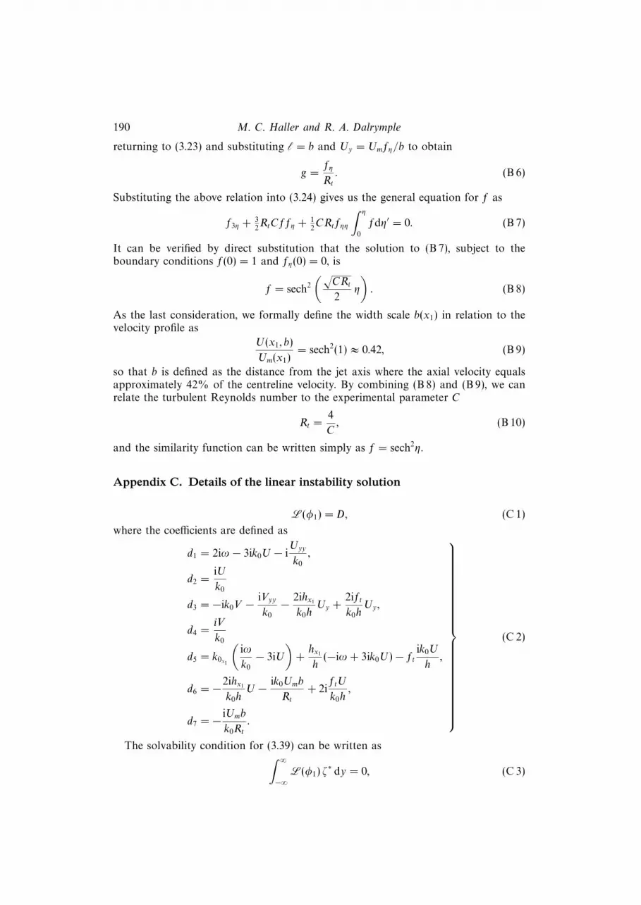
returning to (3.23) and substituting ` = b and Uy = Umfη/b to obtain

g =fη

Rt. (B 6)

Substituting the above relation into (3.24) gives us the general equation for f as

f3η + 32RtCffη + 1

2CRtfηη

∫ η

0

fdη′ = 0. (B 7)

It can be verified by direct substitution that the solution to (B 7), subject to theboundary conditions f(0) = 1 and fη(0) = 0, is

f = sech2

(√CRt

2η

). (B 8)

As the last consideration, we formally define the width scale b(x1) in relation to thevelocity profile as

U(x1, b)

Um(x1)= sech2(1) ≈ 0.42, (B 9)

so that b is defined as the distance from the jet axis where the axial velocity equalsapproximately 42% of the centreline velocity. By combining (B 8) and (B 9), we canrelate the turbulent Reynolds number to the experimental parameter C

Rt =4

C, (B 10)

and the similarity function can be written simply as f = sech2η.

Appendix C. Details of the linear instability solution

L(φ1) = D, (C 1)

where the coefficients are defined as

d1 = 2iω − 3ik0U − iUyy

k0

,

d2 =iU

k0

d3 = −ik0V − iVyyk0

− 2ihx1

k0hUy +

2iftk0h

Uy,

d4 =iV

k0

d5 = k0x1

(iω

k0

− 3iU

)+hx1

h(−iω + 3ik0U)− ft ik0U

h,

d6 = −2ihx1

k0hU − ik0Umb

Rt+ 2i

ftU

k0h,

d7 = − iUmb

k0Rt.

(C 2)

The solvability condition for (3.39) can be written as∫ ∞−∞L(φ1) ζ

∗ dy = 0, (C 3)

Rip current instabilities 191

where we have substituted the following expression for the eigenfunction

φ0 = A(x1)ζ(y; x1), (C 4)

where A(x1) is the amplitude of the disturbance and varies in the axial direction.Direct substitution for D from (C 2) into (C 3) gives∫ ∞

−∞[d1(Ax1

ζ + Aζx1) + d2(Ax1

ζyy + Aζx1yy) + d3Aζy + d4Aζyyy] φ∗0

+

∫ ∞−∞

[d5Aζ + d6Aζyy + d7Aζyyyy] φ∗0 = 0, (C 5)

and this can be rearranged to obtain the following evolution equation for A(x1),

Ax1= ik1(x1)A (C 6)

where

k1 =

i

∫ ∞−∞

(d1ζx1+ d2ζx1yy + d3ζy + d4ζ3y + d5ζ + d6ζyy + d7ζ4y)φ

∗0 dy∫ ∞

−∞(d1ζ+d2ζyy)φ

∗0 dy

, (C 7)

and the terms d1 to d7 are defined by (C 2).

C.1. Numerical method

The boundary conditions for the eigenvalue problem described by (3.38) are asfollows:

φ0 = φ0y → 0 as y → ±∞, (C 8)

φ0y = 0 at y = 0→ sinuous mode,

φ0 = 0 at y = 0→ varicose mode.(C 9)

In order to implement the boundary condition (C 8) at a finite value of y, we usethe conditions U,Uyy → 0 as y → ∞ to obtain the asymptotic form of (3.38). Givenan ω and an initial guess for k0, the solution (φ0 = exp (−k0y)) to the asymptoticequation is applied at a sufficiently large y and then (3.38) is integrated (shootingmethod) using a fourth-order Runge–Kutta algorithm (Hoffman 1992). At y = 0, theboundary condition (C 9) is evaluated, and k0 is iterated using the secant methoduntil the wavenumber is found which satisfies the boundary condition.

With k0 known, (3.42) is integrated using a similar procedure; however, only oneiteration is necessary since the adjoint problem has the same eigenvalues as the originalproblem. The calculation of φ∗0 can then be used as a check on the accuracy of thecomputed eigenvalues. Equation (3.40) is also integrated using a similar procedure.The step size for the numerical integration procedure was generally ∆y = 0.0005b(x1),and, therefore, varied in the axial direction. The distance from the jet axis where (C 8)was implemented was y = 6b(x1).

REFERENCES

Aagaard, T., Greenwood, B. & Nielsen, J. 1997 Mean currents and sediment transport in a ripchannel. Mar. Geol. 140, 25–45.

Arthur, R. S. 1950 Refraction of shallow water waves: the combined effect of currents andunderwater topography. In Eos Trans. AGU, 31, 4, 549–551.

192 M. C. Haller and R. A. Dalrymple

Arthur, R. S. 1962 A note on the dynamics of rip currents. J. Geophys. Res. 67, 2777–2779.

Bickley, W. 1939 The plane jet. Phil. Mag. Ser. 7, 727–731.

Bowen A. J. 1969 Rip currents, 1. Theoretical investigations. J. Geophys. Res. 74, 5467–5478.

Bowman, D., Arad, D., Rosen, D. S., Kit, E., Goldbery, R. & Slavicz A. 1988 Flow characteristicsalong the rip current system under low-energy conditions. Mar. Geol. 82, 149–167.

Dalrymple, R. A. 1975 A mechanism for rip current generation on an open coast. J. Geophys. Res.80, 3485–3487.

Dalrymple, R. A. & Lozano, C. J. 1978 Wave–current interaction models for rip currents.J. Geophys. Res. 83, C12, 6063–6071.

Dodd, N. & Falques A. 1996 A note on spatial modes in longshore current shear instabilities.J. Geophys. Res. 101, C10, 22 715–22 726.

Drazin, P. G. & Howard L. N. 1966 Hydrodynamic stability of parallel flow of inviscid fluid. InAdvances in Applied Mechanics (ed. G. Kuerti), vol. 7, pp. 1–89. Academic.

Falques, A. & Iranzo V. 1994 Numerical simulation of vorticity waves in the nearshore. J. Geophys.Res. 99, C1, 825–841.

Garg, V. K. & Round G. F. 1978 Nonparallel effects on the stability of jet flows. J. Appl. Mech. 45,717–722.

Gaster, M. 1962 A note on the relation between temporally-increasing and spatially-increasingdisturbances in hydrodynamic stability. J. Fluid Mech. 14, 222–224.

Greenberg, M. D. 1988 Advanced Engineering Mathematics. Prentice–Hall.

Haller, M. C. & Dalrymple R. A. 1999 Rip current dynamics and nearshore circulation. Res. Rep.CACR-99-05 (also PhD thesis), Center for Applied Coastal Research, University of Delaware,Newark.

Haller, M. C., Dalrymple, R. A. & Svendsen I. A. 2000 Experiments on rip currents and nearshorecirculation: data report. Res. Rep. CACR-00-04, Center for Applied Coastal Research, Uni-versity of Delaware, Newark.

Hoffman, J. D. 1992 Numerical Methods for Engineers and Scientists. McGraw–Hill.

Huntley, D. A. & Short, A. D. 1992 On the spacing between observed rip currents. Coastal Engng17, 211–225.

Iwata, N. 1976 Rip current spacing. J. Ocean. Soc. Japan 32, 1–10.

Joshi, P.B. 1982 Hydromechanics of tidal jets. J. Waterways, Port, Coast. Ocean Engng 108, WW3,239–253.

Kobayashi, N., Karjadi, E. A. & Johnson, B. D. 1997 Dispersion effects on longshore currents insurf zones. J. Waterways, Port, Coast. Ocean Engng 123, 240–248.

Mei, C. C. 1989 The Applied Dynamics of Ocean Surface Waves. World Science, River Edge, NJ.

Nayfeh, A. H., Saric, W. S. & Mook, D. T. 1974 Stability of non-parallel flows. Arch. Mech. 26,401–406.

Schlichting, H. 1933 Laminare Strahlenausbreitung, Z. Angew. Math. Mech. 13, 260–263.

Shepard, F. P., Emery, K. O. & La Fond, E. C. 1941 Rip currents: a process of geologicalimportance. J. Geol. 49, 337–369.

Slinn, D. N., Allen, J. S., Newburger, P. A. & Holman R. A. 1998 Nonlinear shear instabilitiesof alongshore currents over barred beaches. J. Geophys. Res. 103, 18 357–18 379.

Smith, J. A. & Largier, J. L. 1995 Observations of nearshore circulation: rip currents. J. Geophys.Res. 100, 10 967–10 975.

Sonu, C. J. 1972 Field observation of nearshore circulation and meandering currents. J. Geophys.Res. 77, 3232–3247.

Tam, C. K. W. 1973 Dynamics of rip currents. J. Geophys. Res. 78, 1937–1943.

Tennekes, H. & Lumley, J. L. 1972 A First Course in Turbulence. MIT Press.

Wilmott, C. J. 1981 On the validation of models. J. Phys. Oceanogr. 2, 219–232.

Yoon, S. B. & Liu P. L.-F. 1990 Effects of opposing waves on momentum jets. J. Waterways, Port,Coast. Ocean Engng 116, 545–557.