DOCUMENTO DE DISCUSIÓN

DD/11/08

“Risk Preferences and Demand for Insurance in Peru:

A Field Experiment”

Francisco B. Galarza y Michael R. Carter

© 2011 Centro de Investigación de la Universidad del Pacífico DD/11/08

Documento de Discusión

Risk Preferences and Demand for Insurance in Peru: A Field Experiment

Francisco B. Galarza* Universidad del Pacífico

Michael R. Carter** University of California, Davis

Enero 2011

Abstract

This paper reports the results of behavioral economic experiments conducted in Peru to examine the relationship

amongst risk preferences, loan take-up, and insurance purchase decisions. This area-based yield insurance can

help reduce people's vulnerability to large scale covariate shocks, and can also lower the loan default

probability under extreme negative covariate shocks. In a context of collateralized formal credit markets, we

provide suggestive evidence that insurance may help reduce the fear of losing collateral that prevents potential

borrowers from taking loans. Framing these experiments to recreate a real life situation, we started with a

Baseline Game where subjects had to choose between a fallback production project and an uninsured loan. We

then introduced a third project choice, loan with yield insurance (Insurance Game), which allows us to measure the

effect of introducing insurance on the demand for loans. Overall, more than 50 percent of the subjects are willing to

buy insurance in this insurance game. Further, controlling for the number of peers in the agricultural network,

wealth, and choices made in the baseline game, we find that the project choice decision is predicted by a judgment

bias known as hot-hand effect, and risk aversion. In the latter case, the shape of the relationship is quadratic,

meaning that highly risk averse subjects will prefer switching to the risky, uninsured loan project, while those

showing a low and moderate risk aversion will stick to the safer (fallback or insured loan) projects.

Keywords: area-yield insurance, credit, covariate risk, idiosyncratic risk, risk

aversion, experimental economics, Peru.

JEL codes: C93, D81.

E-mail de los autores: galarza_fb@up.edu.pe, mrcarter@ucdavis.edu

*Contact author. Department of Economics, Av. Sanchez Cerro 2141, Jesus Maria, Lima, Peru. Telephone: + 511.219.0100.

**Department of Agricultural & Resource Economics, One Shields Avenue 2366, Davis, CA 95616. Telephone: +1.530.752.4672.

***Acknowledgments. We thank Brad Barham, Jed Frees, Paul Mitchell, and Laura Schechter for helpful comments as well as seminar

participants at the Universidad del Pacifico (Lima-Peru), Universidad Francisco Marroquín (Guatemala), UW-Madison Development

Seminar, Wesleyan University, and the 2010 Agricultural & Applied Economics Annual Meeting. Steve Boucher, Carlos de los Ríos,

Conner Mullally, and Carolina Trivelli provided helpful feedback on the experimental design. Ramón Díaz, Oscar Madalengoitia, Roberto

Piselli, Chris Rue, Raphael Saldaña, Jessica Varney, Josh Weinberg, and especially Johanna Yancari, provided a valuable assistance in the

field. Financial support from the USAID Cooperative Agreement EDH-A-00-06-0003-00 through the Assets and Market Access

Collaborative Research Support Program is gratefully acknowledged. The usual disclaimer applies.

1 Introduction Risk is widespread in less developed economies, where low-income people living in rural areas are

exposed to several potentially catastrophic hazards, such as severe weather events, which are often

more detrimental than the series of idiosyncratic shocks that periodically affect them. In order

to manage and deal with risk, those people have traditionally used a series of ex-ante and ex-

post strategies,1 with less than desired results. Despite the substantial efforts made to reduce their

vulnerability to negative economic shocks, recent evidence suggests that the consumption variability

at the individual level still remains high in the developing world (Dercon, 2005; Morduch, 1995).

Depending on the nature and magnitude of those shocks, this lack of appropriate equipment may

lead people to chronic poverty, thus affecting their possibilities to engage in an economically viable

growth path.2

In addition to individual specific efforts displayed to handle risk, innovative financial products,

such as uncollateralized microloans and index-based insurance, have been designed and implemented

from the supply side. On the one hand, in the wake of the so-called microfinance revolution, poor

people, typically unable to offer collateral, have become eligible to get credit access and take

advantage of business opportunities. On the other hand, moral-hazard proof insurance written on

average aggregate indices has emerged with the promise of helping households keep valuable assets

which could otherwise be lost as a result of extreme negative shocks.

Besides smoothing consumption over time, index-based insurance may also have an appealing

property in a scenario where a significant proportion of potential borrowers are discouraged from

applying for loans because of their fear of losing collateral in case of default: by reducing the

likelihood of a loan default, it may stimulate a proportion of those fearful producers to enter the

credit market. Given that such voluntary withdrawing from the credit market, termed as risk

rationing (Boucher et al., 2008), has been shown to be an empirically relevant phenomenon in

Peru, where we conduct our research,3 it is expected that the introduction of such an insurance

scheme would have a positive effect on the expansion of the credit market.

The extent to which insurance can help expand credit markets in less developed countries is an

empirical question that has not suficiently been investigated. With only a few index-based insurance

programs operating in less developed countries, the literature on the linkage between credit and

index insurance (or any type of insurance for that matter) is at best scant. To our knowledge, with

the probable exceptions of a handful of works,4 no other study has addressed, directly or

1 Risk management, ex-ante strategies, may include income diversification, savings, insurance, participation in

rotating saving and credit associations (ROSCAs); while risk coping, ex-post strategies, may include the use of

informal loans, liquidation of assets, and reallocation of labor, among others. 2 The literature on poverty has documented this case, in which when households fall below certain threshold—the

Micawber Frontier—their prospects to escape from poverty are negligible (Carter and Barrett, 2006). 3 In Peru, Honduras, and Nicaragua, risk rationed borrowers account for between 12 and 19 percent of the total

sample of borrowers (Boucher et al., 2008). 4 Cole et al. (2008) examined the obstacles to a wider insurance take up in India; Giné and Yang (2009) analyzed

whether rainfall insurance can help increase demand for loans in a randomized control trial in Malawi; Giné et al.

(2009) experimentally tested the demand for different microfinance contracts in urban Peru; and Lybbert (2006)

designed experiments in Morocco to elicit willingness to pay for seeds that increase yields, reduce yields variance or

yields skewness.

2

indirectly, the three issues that concern this paper: the interaction between risk preferences and

demand for credit and insurance.

This paper uses a unique experimental data set gathered in Peru, where we set up an experi-

mental economics laboratory and run experiments that examine the nature and main predictors of

the demand for loans and index-based insurance; we label these behavioral experiments “farming

experiments." We are particularly interested in examining the effect of risk preferences (estimated

in a companion paper, Galarza [2009]) on the decision to purchase an innovative type of crop in-

surance.5 Our farming experiments simulated farming decisions where our experimental subjects

chose among alternative cotton production projects: fallback (low return, or safe), produce with

an uninsured loan (high return, or risky), or produce with an insured loan (less risky ). Using a

payoffs scheme for each project in order to incentivize subjects to reveal their true preferences, this

paper develops an approach that is also used as a tool to build people’s comprehension of this new

insurance product.

A novel feature of this experiment is that projects’ profits depend on the realizations of two

random shocks: a covariate, correlated shock, represented by the valley-wide average yield, and an

idiosyncratic shock. Projects’ profits, constructed using survey data from the Pisco valley, are such

that the uninsured loan does not yield suficient profits to fully repay the loan under a “very low"

realization of the valley-wide average yield, regardless of the realization of the idiosyncratic shock. In

contrast, the insured loan’s profits guarantee full repayment of loans under every realization of the

two random shocks. In order to reproduce the dynamic effects that defaulting on a collateralized

loan involves, we imposed two consequences of not repaying a loan in the experiment: no future

access to loans, and a depreciation of land.

Our sample includes 378 experimental subjects from rural Peru. The experiments started

with a baseline experiment, where farmers had to choose between the fallback project and the

uninsured loan project, in a series of repeated rounds that simulated single farming seasons. We

then introduced the insured loan to the set of choices available (insurance experiment ). This design

allows us testing whether the introduction of insurance affects farmers’ choice between the safe and

the risky project.

Our findings are as follows. First, the experimentally-measured demand for valley-wide average

yield insurance is fairly high: 57 percent of farmers demanded the insured loan project by the last

two high-stake rounds, a proportion that remains rather steady during all the high stakes rounds.

Second, our experimental results suggest that index yield insurance, by reducing the likelihood

of loan defaults, may crowd-in credit markets by a sizeable proportion. We find that about 60

percent of the subjects who chose the fallback, safe project (i.e., 24 percent of the total subjects)

in the baseline experiment switched to the insured loan project in the insurance experiment. This

result indicates that insurance would allow almost 14 percent of the total number of subjects not

5 This research pro ject was carried out in partnership with an insurance company in Peru and a vendor of insurance

contracts bundled with loans that operates in our research site, the Pisco valley. At all times during the course of the

experimental sessions, we emphasized the fact that our participation as researchers was simply intended to inform

farmers about the main features of this new financial product and to examine their willingness to buy it. We also

stressed the fact that participating in these sessions should not make them feel obliged to buy insurance.

3

to withdraw from the credit market.6 While such estimated magnitude may be used with caution,

it is suggestive that insurance could encourage the undertaking of riskier but potentially more

profitable production projects thanks to new funds coming from a loan. Third, controlling wealth

and choices made in the baseline experiment, we find evidence of ‘hot-hand’ effects (stemming from an

underestimation in the autocorrelation of the sequence of ‘very bad’ years) in project choice,

while static risk preferences estimated under Expected Utility Theory (EUT) appear to have a

quadratic (concave) relationship with project choice, meaning that highly risk averse subjects will

prefer switching to the risky project (uninsured loan), while those showing a low and moderate risk

aversion will stick to the safer (fallback or insured loan) projects. This result offers novel evidence

about the relationship between risk aversion and preferences for innovative financial instruments.

The remainder of this paper is organized as follows. Section 2 discusses our experimental design

in the context of related works. Section 3 describes the experimental procedures followed and the

data used; and also presents a descriptive analysis of the results. Section 4 analyzes the main

econometric results and Section 5 concludes.

2 Related Studies and Our Experimental Design In this section, we review the literature relevant to our research (section 2.1) and then discuss the

distinctive features of our experimental design in that context (section 2.2). Using the terminology

coined by Harrison and List (2004), our farming experiments are framed field experiments, as they

concern valuations over a real commodity (cotton) and involve tasks similar to those performed by

the experimental subjects acting in their usual production environment.

2.1 Related Studies

In recent years, we have witnessed a rapid growth in the number of experimental studies in devel-

opment economics. Although these works have analyzed a wide gamut of topics, there still remains

much to be done in terms of applying the laboratory experimental tools in the analysis of develop-

ment issues. In a survey of the literature about experiments conducted in less developed countries,

Cardenas and Carpenter (2005) report that three of the main topics studied are the measurement

of trust, cooperation, and risk preferences; none of these studies investigates the role of elicited risk

preferences in explaining the demand for financial contracts.

A more recent set of behavioral field experiments that concern the topics analyzed in this paper

involve testing the demand for microfinance contracts (Giné et al., 2009) and the willingness to pay

for seeds that stabilize yield distributions (Lybbert, 2006), using in both cases a payoffs scheme to

incentivize subjects’ truthful preference elicitation. Two other works that used randomized control

trials to examine the demand for weather-based insurance in India and Malawi, respectively (Cole

et al., 2008; Giné and Yang, 2010), will also be discussed below.

6 After this round in default, farmers are left with no choice but to do the fallback pro ject. The quantitative

importance of this finding increases to about 20 percent when we use the modal choice during the high-stake rounds.

4

Lybbert (2006) investigates farmers’ preferences about three desirable properties of cotton seeds

in India: an increase in average yields, a reduction in yields’ variance, and a reduction in yields’

skewness. Using the Becker-DeGroot-Marchak method (Becker et al., 1964) to elicit the maximum

willingness to pay for those traits, where farmers were given the payoff distributions related to each

type of seed before making their bid,7 Lybbert shows that farmers value seeds that increase the

expected returns, but no evidence about their valuation of the other two traits of seeds was found.

As Lybbert acknowledges, the lack of valuation of yield’s risk reduction (i.e., less variance) may be

explained by the inability of the experimental design to control for the relevant factors that affect

farmer’s valuation of crop yield distributions. Lybbert’s results further show no statistically strong

relationship between any individual characteristic (such as wealth) and expected returns, a result

that the author claims could be due to the existence of credit constraints.

Giné and Yang’s (2010) randomized control trial in Malawi examine whether insurance can

induce farmers to take loans to adopt a new, high-yielding seed variety. The control group was

offered a loan to purchase a high-yielding seed; while the treatment group was offered an identical

loan contract but was required to buy actuarially fair rainfall-indexed insurance if they took the

loan. This insurance can allow to partially or fully repay the loan, depending on how low the rainfall

is. Thus, while assuming a risk averse behavior, one could expect insured farmers to be more willing

to take out a loan in order to undertake a potentially more profitable investment (i.e., buying the

high-yielding seed), Giné and Yang find exactly the opposite result: loan take-up rates are much

lower for the treatment group (17.6 percent versus 33.0 percent). The authors suggest that the

low insured loan take-up could be due to the prior existence of limited liability; that is, the actual

consequences of defaulting on a loan might not have been so severe in the first place, and thus the

actual value of buying insurance would be limited. In the same line, Cole et al.’s (2008) randomized

control trials in India aim to identify the barriers to a wider adoption of rainfall insurance. They

find that subjects’ purchase rates are very price elastic, and that cash constraints seem to play a

role in insurance adoption. More interestingly, they find that third party endorsement (such as

that of a local authority) of insurance can affect its take-up, thus suggesting a potentially strong

correlation between choices across subjects from the same village.

Our behavioral experiment shares some features in common with the previously discussed works,

but it arguably offers a more complete depiction of how rural producers make production decisions.

In particular, our experiment focuses on examining the interrelationship among three themes:

agricultural yields, loan, and insurance. In our experiment, loans yield higher expected yields (i.e., a

more profitable production) and insurance eliminates the possibility of defaulting on a loan, thus

securing the farm production and ensuring farmers to keep access to loans in the future. Written

on valley-wide yields, this insurance protects producers from catastrophic events that dramatically

reduce average yields at the valley level. Subjects’ farming profits depend on two random variables:

7 Once farmers bid a price, a random seed price was drawn from a uniform distribution with mean of 50 Rupees

(Rs.). Thus, if farmers bid at least the amount of the randomly drawn price, they could get the seed and “plant

it", and get the corresponding payoff. After this, farmers draw a chip from a bag to determine the season’s harvest

payoff. Thus, for a farmer who planted the seed, his net earnings would be the harvest payoff, minus the price paid

for the seed, plus 50 Rs. (off-farm earnings), while for one who did not plant the seed, it would be only the 50

Rs. corresponding to the off-farm earnings.

5

a covariate shock—represented by the valley-wide average yield—that affects equally all subjects

in the same valley, and an idiosyncratic shock, uncorrelated with the covariate shock.

Moreover, while our farming experiments are close in spirit to the randomized control trials

conducted by Giné and Yang (2010), we used actual payoffs to incentivize players to elicit their

preferences for distinct production projects. Moreover, our farming experiments have greater com-

plexity than the experiments of Lybbert (2006) in that our farmers’ payoffs for each project choice

depend on two sources of randomness, while in Lybbert’s experiments there is only a random

“yield risk" that subjects should consider before deciding their choice (a seed). Likewise, our farm-

ing experiments introduce additional complexity to the typical individual loan experiments, in

which players have to choose whether to request a loan with a risky result, or to invest in a safe

project (e.g., Giné et al., 2009), by providing subjects a more complete set of financial instruments

to finance their production. Obviously, the greater complexity in the design of our experiments

increases the challenges for ensuring experimental control. In the next section, we discuss our

experimental design.

2.2 Our Farming Experiments

The experiment script for our farming experiments was written following standard experimental

procedures as close as possible (Davis and Holt, 1993). Experiment trials were conducted in Madison

and Davis in the U.S. (with graduate students), and Lima (with social scientists and cotton farmers),

and the valley of Pisco and its neighbor Ica (with cotton farmers), in Peru. The final version of

the script was reviewed by a journalist who works closely with farmers, in order to ensure that the

language used in the instructions would be understandable to a typical farmer.

The farming experiments were designed to examine the potential demand for index-based crop

insurance and analyze the effects of buying insurance on the demand for loans. In these experiments,

we simulated farming decisions where subjects, endowed with a “hectare of land", had to choose

among alternative cotton production projects—fallback (safe project), take an uninsured loan (risky

project), and take a loan bundled with index yield insurance (insured loan, less risky project)8 —in

a series of repeated rounds.

Each project yields a related profit, which is known to subjects before they make their decisions.

In the cases of the uninsured loan and the insured loan projects, profits depend additively on the

realization of two random variables: a covariate shock (represented by the valley-wide average yield),

and an idiosyncratic shock. The probability distributions of both shocks were estimated using

information from the Pisco valley. In particular, detrended 1986-2006 time series data of valley

yields (yt), expressed in Kilograms per hectare, were fitted to a Weibull density function. The

parameters of the Weibull function were estimated using maximum likelihood in Gauss:9

yt ~ Weibull (6.00, 1806.08), (1)

8 Throughout the paper we use interchangeably the terms fallback, and safe pro ject; the terms unisured loan and

risky pro ject, and the terms insured loan and loan bund led with yield insurance pro ject. 9 We used the Broyden–Fletcher–Goldfarb–Shanno (BFGS) algorithm. The parameters’ standard deviations are

1.03 and 70.17.

6

which has mean of 1,674 Kilograms per hectare.

Moreover, four-year (2002-2005) panel data were used to estimate the distribution of the idio-

syncratic shocks ( it),10 using the following fixed effects model:

yit - µi = βi(yt - µ) + εit; (2)

which regresses the farmer i’s yields (yi) deviation from its mean, µi, on the deviation of the

sample ’s average yields (yt) from its mean (µ).

We then discretized the densities of valley yields; yt11 (Weibull), and idiosyncratic shocks, it

(Normal distribution, centered on zero), in order to simulate the effects of distinct realizations of

those shocks on profits. In particular, we divided the density of yt into five sections—labeled as very

low, low, normal, high, very high —having the following probabilities (in percent): 10, 20, 40, 20,

and 10. Analogously, the density of it was divided into three sections—labeled as bad, normal,12

and good —with the following probabilities: 25, 50, and 25.

Once we performed the estimations above, all yield figures were converted to quintals (QQ)13

(1 quintal = 46 Kilograms), a denomination familiar to our subjects. Thus, the valley average yield

values, yt, corresponding to the mid-point of those sections are (in rounded figures): 23, 30, 37,

43, and 48 quintals per hectare, respectively. In the case of the idiosyncratic shocks, we consider

the deviations from the “normal" category, expressed as ∆εit, in the computation of the profits.

In particular, the mid-point of the “bad" luck category lies –12.12 percent (below) the center of

the distribution of, while the mid-point of the “good" luck category lies 11.63 percent above the

center of the distribution.

The farmer i’s per hectare profits in Soles from the insured and uninsured loan projects at

each section of the valley yield and idiosyncratic shock densities, was computed using the following

formula:

Пitproject

= (p . yt) * (1 + ∆εit) - (1 + r)Loan + p* I ndemnity - premium; (3)

where the price (p) of a quintal of cotton is set at 124.2 Soles, the loan size (Loan) used is 2,464

Soles (equivalent to US$800 at the time of conducting the experiment), and the interest rate (r)

was set at 30 percent (the going rate at that time). Insurance contract is written on 85 percent of

the average valley yields, equivalent to 31 quintals per hectare (=1,674/46 = 36.4 x 0.85)14 and the

premium was set at 150 Soles per insured hectare.15 Thus, the Indemnity (expressed in quintals

per hectare) in period t is defined as I (yt < 31) * (31- yt), where I(.) is the indicator function.

This indexed insurance thus covers any shortfall in valley average yields below the 31 quintals per

1 0 This is also a measure of the uninsured, or basis risk, uncovered by insurance. 1 1 Note that y represents the valley average yield, while y refers to the sample average used to estimate the

idiosyncratic shocks. 1 2 The “Normal" categories of those shocks lie roughly at the center of their respective densities. 1 3 A Quintal is equivalent to 100 pounds, which is in turn roughly equivalent to 46 Kilograms. 1 4 This strike yield was set after game trials in Pisco, where most sub jects preferred the 85 percent strike yield over

the 65 percent and 90 percent strike yields. 1 5 This premium includes a mark-up or load of 40 percent over the actuarially fair price (107 Soles per hectare).

7

Ind

em

nific

ation

P

aym

en

ts,

So

les/h

ecta

re

Yie

lds D

en

sity

hectare, as depicted by the solid line in Figure 1, where we also plot the estimated Weibull density

of the average valley yields. The indemnity function for the 100 percent contract (dotted line),

with a strike yield of 36.4 quintals per hectare, is also pictured for comparison.

Figure 1: Indemnity and Valley Yield Density Functions for Pisco

1200

1000

100% Strike Point

Estimated Probability Distribution

for Average Yields

800

600

400 85% Strike Point

200

0

20 30 40 50 60

Cotton Yields, Quintals

Furthermore, in order to simplify the implementation of the experiment, we considered the

case of the typical farmer (i.e., βi = 1), which basically implies a one-to-one relationship between

individual farmer’s yields (yit) and actual average valley yields (yt), using the expression indicated in

eqn.[2]. The figures of individual yields used in the profit function shown in eqn.[3] then correspond

to the mid-point value of the valley yields at every section of its density (23, 30, 37, 43, and

48 quintals per hectare, going from “very low" to “very high" yields): yit = yt. The resulting

profit figures were rounded to the nearest 50. For the fallback project, profits were adjusted

accordingly to get lower but more stable profits than in the uninsured loan case.16 We will discuss the

characteristics of the resulting profits for each project in the next section.

As mentioned earlier, our behavioral experiments consisted of a sequence of two sets of experi-

ments. We started with a baseline experiment, where farmers had to opt for either the fallback or

the uninsured loan project. And then, we continued with an insurance experiment, where a third

alternative project (insured loan) was included in the set of choices. This sequential structure of

the experiments allows us to examine any changes in farmers’ choices between the first two projects

after the introduction of insurance.

An important characteristic of the uninsured loan project is that when the valley average yield

1 6 We further assumed a symmetric distribution for the idiosyncratic shock around the mean of zero.

8

is very low, the farming income is not suficient to repay the loan, regardless of the idiosyncratic

shock. Defaulting on a loan involves two negative consequences in the experiment: no future access

to credit (i.e., subjects must do the fallback project) and a 50 percent decrease in the value of the

“endowed" land. The value of a hectare of land was set at 2,400 Soles; the reduction of this value

to 1,200 Soles is meant to simulate the penalty that would occur after defaulting on a collateralized

loan. On the other hand, buying the (85 percent) insurance contract guarantees the full repayment

of loans at every realization of the valley average yield and the idiosyncratic shock, thus allowing

farmers to keep the option of choosing the uninsured loan project in the future and to preserve

their land value.

In the next section, we describe in detail the procedures followed in the implementation of these

farming experiments.

3 Experimental Procedures and Data Our experimental design faced two major challenges: to explain clearly the notion of probabilities

associated with the different sections of the probability distributions for the covariate and idio-

syncratic shocks, and to ensure a minimum level of comprehension of the insured and uninsured

loan projects, so that choices would be “informed." We responded to the first challenge by using

transparent randomizing devices to simulate the realizations of the covariate shocks (colored chips)

and idiosyncratic shocks (colored ping-pong balls), which were referred to as “individual luck," in

order to convey the idea that their individual characteristics are uncorrelated among peers within

a given valley. These shocks were drawn from sacks containing 10 chips (1 black, 2 red, 4 white, 2

blue, and 1 green)—the “valley sack"—and 4 balls (1 purple, 2 white, and 1 yellow)—the “luck

sack"—which reproduce the probabilities structure mentioned earlier, going from the worst to the

best outcome. The design of the experiment worksheets reinforced the information about the prob-

abilities under each scenario of the covariate shock and idiosyncratic shock, by (i) spacing columns

and rows, respectively, in a roughly proportional manner; and (ii) by including pictures in color of

the actual colored chips and balls associated with each scenario. Table 1 shows a sample worksheet

used for the insured loan project, labeled as project C, in the actual experiments. A similar design,

also printed in color, was used for the other projects’ worksheets. We will discuss the profits’ figures

later.

Secondly, in order to enhance subjects’ comprehension of the procedures, field assistants ex-

plained them how the combination of a covariate shock and an idiosyncratic shock drawn deter-

mined the profits of the project chosen in every decision round, where each round represented a

single farming season. The monitor, in charge of giving the instructions to all participants as a

group, illustrated the rules and procedures with interactive examples. We also allowed participants

to ask questions during the course of the presentation of the instructions.17 We were aware of the

risks of doing this, but we actually did not receive questions that may have induced players to play

1 7 Key moments at which we specifically asked if they had any questions were: at the end of the pro ject description,

and before the low- and high-stake rounds.

9

Table 1: Sample Game Worksheet used for Project C

in a certain way.18

The experiment instructions were read aloud in Spanish by the same monitor in every session.

The monitor used a projector to present the information about the types of shocks, the projects’

characteristics and the sequence of the actions subjects should follow in each decision round. The

contents of those slides are provided in Appendix A.19 At the beginning of every session, all par-

ticipants received a binder containing the worksheets with the information of the projects’ profits

related to each type of covariate and idiosyncratic shocks, as well as a pencil to record their choices, the

type of shocks realized, and the resulting profits in each simulated farming season. Helping

subjects to see the connection between their choices, types of shocks drawn, and resulting profits,

was also intended to enhance trust in our calculations of their experiment winnings.

The farming experiment lasted three hours on average. Total experiment winnings in cash from

participating in this particular experiment ranged from 11 to 26 Soles, with average winnings of

17 Soles (equivalent to $6). Experiment winnings and attendance fees were paid at the end of

the entire session—which also included the conduct of the risk experiment (results are reported

in Galarza [2009]), and pre-experiment and post-experiment surveys—that lasted on average five

hours.20

Recall that in all of our 24 sessions, participants were assigned to numbered seats at random

upon arrival, and we divided the participants into at most four “valleys" with a minimum of 3

members in subjects’ each one. Splitting subjects this way allowed us to get more variability in the

realizations of the covariate shocks, to have a closer monitoring, and to accelerate the tasks. Two

persons from our field team were in charge of each valley. A senior assistant, well versed in the

1 8 Most of the questions asked concerned the reasons for the differences in payoffs from particular pro jects

under certain realizations of shocks; whether yield insurance covered losses due to hazards at the irrigation sector

level; the source of the (agricultural production, cost, and valley yield) figures used for our analysis; whether the

indemnity payments could be suficient to repay the loan; or the timing of the insurance payouts; and the like. 1 9 Out of the 24 sessions held, only in three of them we used posters containing the same information as in the

slides for a short time. The monitor used sixteen slides to explain the farming and risk games. 2 0 After finishing the farming experiments and having a short break, a risk experiment—which lasted about 30

minutes on average—was ran. The rest of the time—one hour and a half—was spent conducting the entry and exit

surveys.

10

L Bad [0.25 ] u Normal [0.50 ] c Good [0.25 ] k Mean

experiment rules and procedures, recorded the players’ choices and profits, and did the entry and

exit surveys, while a helper assisted with the drawing of the covariate and idiosyncratic shocks.

Let us consider now the structure of profits associated with each type of covariate and idio-

syncratic shock that was shown to our subjects. Table 2 reports the profits calculated without

considering the probability of losing land. As seen in the table, the uninsured loan project (labeled

as project A) has higher, but more volatile, expected profits than the other two projects; with the

fallback project (project B) being the least profitable project in expectation and the one with the

lowest standard deviation (the safest). More specifically, the mean profits of the projects are: 1,355

(project A), 735 (project B), and 1,283 (project C), while their standard deviations—reported in

Table 3, columns 2 to 4—are 859, 331, and 767, respectively.

Table 2: Farming Game Profits

(Expressed in Soles per hectare)

Valley-Wide Average Yield

Very Low Low Normal High Very High Mean (23 QQ) (30 QQ) (37 QQ) (43 QQ) (48 QQ) [0.10 ] [0.20 ] [0.40 ] [0.20 ] [0.10 ]

Project A: Produce cotton with loan (uninsured loan)

0 1 250 800 1,350 2,000 840 0 1 600 1,400 2,100 2,700 1,370 0 1 900 1,900 2,800 3,400 1,840 0 588 1,375 2,088 2,700 1,355

Project B: Produce cotton without a loan (fallback)

L Bad [0.25 ] 300 400 600 900 1,350 665 u Normal [0.50 ] 350 450 650 1,000 1,500 735 c Good [0.25 ] 400 500 700 1,100 1,650 805 k Mean 350 450 650 1,000 1,500 735

Project C: Produce cotton with a loan & insurance (insured loan)

L Bad [0.25 ] 150 150 650 1,200 1,850 730 u Normal [0.50 ] 500 500 1,250 1,950 2,550 1,295 c Good [0.25 ] 850 850 1,750 2,650 3,250 1,810 k Mean 500 500 1,225 1,938 2,550 1,283

Note: Subjects were shown this table, except for the averages and probabilities. 1 The values of unpaid debts were 700 (Bad luck), 350 (normal luck), and 50 (good luck).

On the other hand, considering the probability of losing land (i.e., of losing 1,200 Soles when

project A is chosen and a very low valley yield is realized) in the calculation of projects’ profits, the

mean profit of the insured loan project becomes now the largest. To make the figures comparable

with those shown in the previous table, we only changed the profits for project A under the very

low average yield (reported a net loss of –1,200 instead of 0), while in the other two projects, no

land losses are realized. As a result, while insurance only decreases the standard deviation of profits

11

from 859 to 76721 when no land losses are considered (see columns 2 and 4 of Table 3), we can see

a much greater reduction in volatility when land losses are included in the profits calculation (from

1,099 to 767 in their standard deviations22 ). While we can easily notice that the expected benefits

from buying insurance would be even greater in an intertemporal context, in which the land not

lost would yield potentially greater profits, it is likely that our subjects did not perceive this effect

to its full extent.23

Thus, we will argue that risk aversion considerations could better guide an ordering in pref-

erences. One could then state that as risk aversion goes up, subjects would tend to switch from

the uninsured loan (A) to the insured loan project (C), and then to the fallback project (B). This

ordering, which also corresponds to the ranking according to the standard deviation of the three

projects’ profits shown in Table 3, will be used as the base ordering in the econometric analysis

performed in Section 4. We could use the ordering according to the total expected profits in future

analysis.

Table 3: Farming Game Payoffs: Mean and Standard Deviation

(Expressed in Soles per hectare)

Excluding Land Loss Including Land Loss1

Unins.Loan

(Project A) Fallback

(Project B) Ins. Loan

(Project C) Unins.Loan

(Project A) Fallback

(Project B) Ins. Loan

(Project C)

Mean 1,355 735 1,283 1,235 735 1,283 Stand.Dev. 859 331 767 1,099 331 767

Ordering considering: Mean 1st 3rd 2nd 2nd 3rd 1st Std. Dev. 3rd 1st 2nd 3rd 1st 2nd

1 Only the profits from project A under the very low valley yield changed (from 0 to -1,200).

Turning now to the procedures followed during the course of our farming experiments, we started

with the baseline experiment, and continued with the insurance experiment. As is customary in

experimental economics, each of those experiments started with a set of six “low stakes" rounds,

intended to get subjects familiar with the experiment rules and procedures, which were followed by a

set of six “high stakes" rounds. Subjects knew that all sets of rounds would end with the sixth

one.24

In the baseline experiment, subjects chose between the fallback (project B: cotton without a

loan ) and the uninsured loan (project A: cotton with a loan ) projects. The sequence of events in

each round of play, t, was as follows:

2 1 To see more clearly the magnitude in the reduction of profits’ risk, this implies a reduction from 0.63 to 0.60 in

the coeficient of variation of profits. 2 2 Which implies a substantial reduction in the coeficient of variation from 0.89 to 0.60 due to insurance. 2 3 One interesting extension, which is beyond the scope of this paper, would be to consider that farmers use

decision weights instead of ob jective probabilities in their expected calculations and to examine the ranking of mean

and standard deviation of those pro jects. 2 4 After several experiment trials, we chose six rounds because it showed to have suficient variability in the covariate

shocks. In particular, we were interested in getting a very bad valley-wide averge yield in each six-round campaign,

so that farmers would learn first hand the consequences of choosing the loan pro ject.

12

(i) All players selected their favorite projects;

(ii) (starting clockwise in each valley, v) one player drew a covariate shock (represented by a colored

chip) from the valley sack. Players rotated this picking-the-chip role;

(iii) then each player i drew his or her own idiosyncratic shock or “luck" (colored ball) from the

luck sack;

(iv) our assistants explained the profit corresponding to the triplet {project chosenivt, covariate

shockvt, idiosyncratic shockivt} to each subject.

Once the six rounds were played, one of them was randomly chosen for play by having a

participant in each valley roll a six-sided die. We used this random incentive design in order to

preserve the proper incentives to carefully select every choice. This selection criterion of the round

for play was reminded to all subjects at the beginning of each set of six rounds.

Furthermore, in order to include the effects of losing collateral into the decision-making, the

total experiment payoffs included the value of the endowed land at the end of the every set of

six rounds, in addition to the experiment profits obtained from the project chosen. In order to

determine the final land value, we used the following rule: regardless of which round was chosen for

play, as long as in any of them the following combination {uninsured loan; black chip, any

colored ball} resulted, farmers were paid half of the original land price. Subjects’ winnings were

as follows: for every 1,200 Soles of payoffs (profit plus land value), participants would receive 1 Sol

in cash. Subjects learned their winnings in cash at the end of each set of six rounds.

The low-stake rounds were followed by a set of six “high-stake" rounds, where subjects started

again with a clean slate: full access to loans, and a hectare of land with its original value. The

procedures and rules were exactly the same as we described earlier, and the only change was the

increase in 100 percent in the exchange rate to compute the winnings in cash, as a way to incentivize

more careful decisions. Thus, now for every 600 Soles of payoffs, participants would receive 1 Sol

in cash.

After running the baseline experiment, the insurance experiment was conducted; we had again

a set of 12 rounds with the insured loan project (project C: cotton with loan & insurance ) included

in the set of choices. The rules and procedures followed in this new experiment, as well as the

exchange rates used, were exactly the same as the ones described above. We emphasized with

subjects that the results from the baseline experiment (i.e., whether subjects defaulted on a loan or

not) did not carry over to the insurance experiment. Written on 85 percent of the long-run average

valley yields, insurance pays out indemnities when valley yields fall below 31 quintals per hectare;

i.e., when valley yields are “low" (30 quintals per hectare) or “very low" (23 quintals per hectare),

which will happen when a black chip or a red chip are drawn in a valley. We should note in Table 2

that, since indemnity payouts cover exactly the shortfalls under those sections of the distribution,

the amount of the profits are the same for every category of idiosyncratic shock (150, 500 and 850

Soles).

13

3.1 Participants Characteristics and Matrix of Choices

The main characteristics of our experimental subjects are as follows: Our typical experimental

subject is older than 50, has spent half of her lifetime managing a farm, has only completed

elementary education (six years of schooling), owns 6 hectares, sows 5 of them, and holds assets

for twenty thousand Soles (about $7,000), as shown in Table C.1 in the Appendix. Moreover, 66

percent of our subjects have access to any type of credit, only 14 percent of them have life insurance;

and 10 percent, have accident insurance. Furthermore, on average, subjects exhibit a moderate to

high risk aversion. We will examine more closely these variables later on.

It should be mentioned that, since we are interested in capturing the choices that contain the

most information possible, the following analysis will use the last high stakes round at which subjects

stopped learning about the different projects, which is the last high stakes round (if subjects did

not fall in default) or the round immediately prior to the one in which subjects fell in default (given

that immediately after that round, subjects are only left with the fallback project). We call this

round the final unconstrained round.25

Table 4 shows one of our main results, the matrix of project choices made by subjects in the

baseline experiment (indicated in rows) and in the insurance experiment (in columns). We observe

at the bottom of column 5 that a large proportion (57 percent) of the experimental subjects chose

the insured loan project, a proportion that was similar in all of the high stakes rounds. (The

average number of switches in project choices is 0.80, with a standard deviation of 1.31.) Another

interesting result is that purchasing insurance seems to have encouraged almost 14 percent (52

out of 378) of subjects to opt for a loan instead of producing using their own resources (see cell

{B,C} in the matrix), thanks to the reduction in the likelihood of default implied by insurance. An

alternative reading of the same figure indicates that about 60 percent (52 out of 91) of the risk

rationed subjects (i.e., those who chose the fallback project in the baseline experiment26 ) switched

to the insured loan project when it was available. This is an encouraging result that goes in line

with an intended effects of insurance: to encourage farmers to undertake riskier but potentially

more profitable projects.

We can further see in the table that a relatively small proportion of subjects made choices

inconsistent with transitivity in preferences. In particular, 20 out of 91 subjects who selected the

fallback project over the uninsured loan project in the baseline experiment (cell {B,A}) switched

to the uninsured loan project in the insurance experiment, and 14 out of 287 subjects who chose

the uninsured loan in the baseline experiment (cell {A,B}) switched to the fallback project in the

insurance experiment. Note that since we are working with the final unconstrained rounds, these

choices were made before any bad year (i.e., a black chip drawn in a given round) happened when

the uninsured loan was selected, and thereby they are likely to reflect their true preferences.27

2 5 During the first high stake round of the insurance game, 2.6 percent of sub jects went into default. 2 6 Obviously, we are assuming here that these sub jects are risk rationed in real life, a result that may not necessarily

hold. 2 7 Using the modal choice during the high-stake rounds would result in a take-up rate for the insured (uninsured)

loan of 58.5 percent (24.3 percent), and 37.6 percent of risk rationed sub jects, with 57 percent of them switching to

the insured loan in the Insurance Game.

14

Table 4: Choices in Baseline and Insurance Games

Insurance Experiment Uninsured loan

(A) Fallback

(B) Insured loan

(C) Total %

Baseline

Experim

ent

Uninsured loan (A)

% 109

38.0 14

4.9 164

57.0 287

100.0 75.9

Fallback (B)

% 20

22.0 19

20.9 52

57.1 91

100.0 24.1

Total

% 129

34.1 33

8.7 216

57.1 378

100.0 100.0

Before we discuss the main distinctive characteristics of subjects in the baseline and insurance

experiments, we need to define two variables of interest that were constructed from within the

experiments: financial literacy and risk aversion. In constructing this measure of the degree of

comprehension of the main features of the insured and uninsured loans, we included four indicators:

(i) self-reported comprehension of the farming experiment rules (variable Self-report ), (ii) whether

subjects knew (reminded) that insurance indemnity payouts depend on valley-wide average yields

(Learn_ins1 ) and (iii) not on idiosyncratic shocks (Learn_ins2 ), and (iv) whether they knew the

two consequences of defaulting on a loan (Learn_loan ). We assigned the same weights to each of

these variables:

F inancial literacy = (Self -report + Learn_I ns1 + Learn_I ns2 + Learn_Loan)/4;

where Self-report takes the values of 1, 0.75, 0.5, or 0.25 if subjects claimed that the instructions

were “very easy", “easy", “hard", or “very hard", respectively. Learn_Ins1 and Learn_Ins2 are

indicator variables that take the value of 1 if the answer was correct and 0, otherwise. Learn_Loan

takes the value of 1 if the two consequences of defaulting an uninsured loan (i.e., no future access

to loans and land depreciation) were indicated by subjects; 0.5 if only one of those were mentioned;

and 0 otherwise. We then normalized this indicator to take values between 0 (which means that a

subject does not know anything about the rules of the experiment) and 1 (which indicates that a

subject knows very well the rules). The average value of this indicator across subjects is 0.54,

which indicates a moderate level of comprehension overall.28

In the case of elicited risk preferences, risk parameters were estimated using the results of a

lottery experiment conducted with the same Pisco subjects. The data were fitted to Constant Rela-

tive Risk Aversion (CRRA) utility functions under Expected Utility Theory (EUT) and Cumulative

Prospect Theory (CPT),29 resulting in average estimated CRRA coeficients of 0.45 (EUT) and 0.74

2 8 If we excluded the self-reported comprehension variable (self-report ), such an indicator would have an average

value of 0.50, and the correlation coeficient with education would be 0.37. 2 9 Under EUT, risk preferences are entirely defined by the curvature parameter, while in CPT, a probability weight-

ing function parameter also affects risk preferences. This function captures the sub jective distortions made to actual

probabilities. More details of the estimation process are provided in Section 4.1.

15

(CPT), estimates that suggest the existence of a moderate to relatively high degree of risk aversion.

The interested reader is referred to our companion paper (Galarza, 2009) for details.

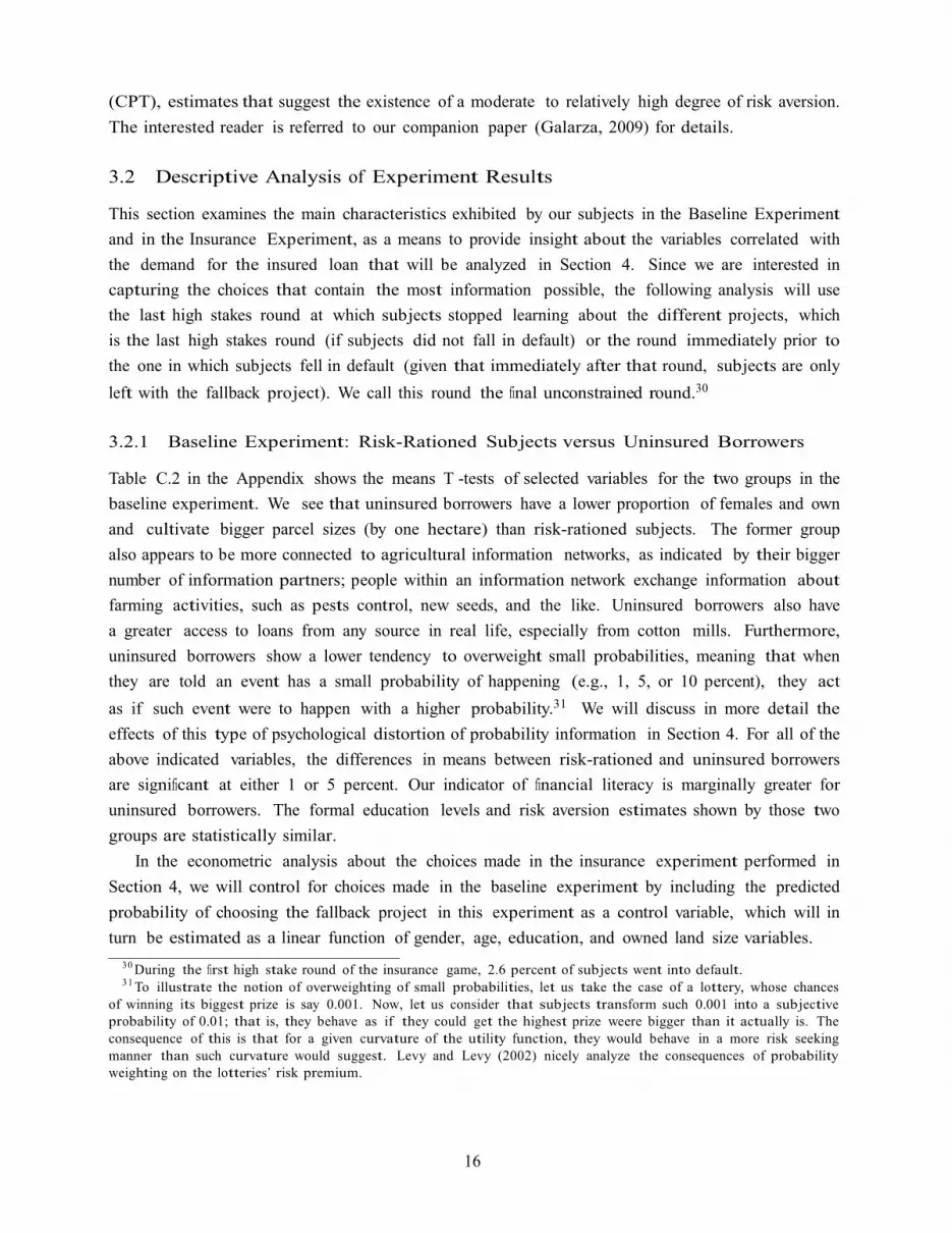
3.2 Descriptive Analysis of Experiment Results

This section examines the main characteristics exhibited by our subjects in the Baseline Experiment

and in the Insurance Experiment, as a means to provide insight about the variables correlated with

the demand for the insured loan that will be analyzed in Section 4. Since we are interested in

capturing the choices that contain the most information possible, the following analysis will use

the last high stakes round at which subjects stopped learning about the different projects, which

is the last high stakes round (if subjects did not fall in default) or the round immediately prior to

the one in which subjects fell in default (given that immediately after that round, subjects are only

left with the fallback project). We call this round the final unconstrained round.30

3.2.1 Baseline Experiment: Risk-Rationed Subjects versus Uninsured Borrowers

Table C.2 in the Appendix shows the means T -tests of selected variables for the two groups in the

baseline experiment. We see that uninsured borrowers have a lower proportion of females and own

and cultivate bigger parcel sizes (by one hectare) than risk-rationed subjects. The former group

also appears to be more connected to agricultural information networks, as indicated by their bigger

number of information partners; people within an information network exchange information about

farming activities, such as pests control, new seeds, and the like. Uninsured borrowers also have

a greater access to loans from any source in real life, especially from cotton mills. Furthermore,

uninsured borrowers show a lower tendency to overweight small probabilities, meaning that when

they are told an event has a small probability of happening (e.g., 1, 5, or 10 percent), they act

as if such event were to happen with a higher probability.31 We will discuss in more detail the

effects of this type of psychological distortion of probability information in Section 4. For all of the

above indicated variables, the differences in means between risk-rationed and uninsured borrowers

are significant at either 1 or 5 percent. Our indicator of financial literacy is marginally greater for

uninsured borrowers. The formal education levels and risk aversion estimates shown by those two

groups are statistically similar.

In the econometric analysis about the choices made in the insurance experiment performed in

Section 4, we will control for choices made in the baseline experiment by including the predicted

probability of choosing the fallback project in this experiment as a control variable, which will in

turn be estimated as a linear function of gender, age, education, and owned land size variables.

3 0 During the first high stake round of the insurance game, 2.6 percent of sub jects went into default. 3 1 To illustrate the notion of overweighting of small probabilities, let us take the case of a lottery, whose chances

of winning its biggest prize is say 0.001. Now, let us consider that sub jects transform such 0.001 into a sub jective

probability of 0.01; that is, they behave as if they could get the highest prize weere bigger than it actually is. The

consequence of this is that for a given curvature of the utility function, they would behave in a more risk seeking

manner than such curvature would suggest. Levy and Levy (2002) nicely analyze the consequences of probability

weighting on the lotteries’ risk premium.

16

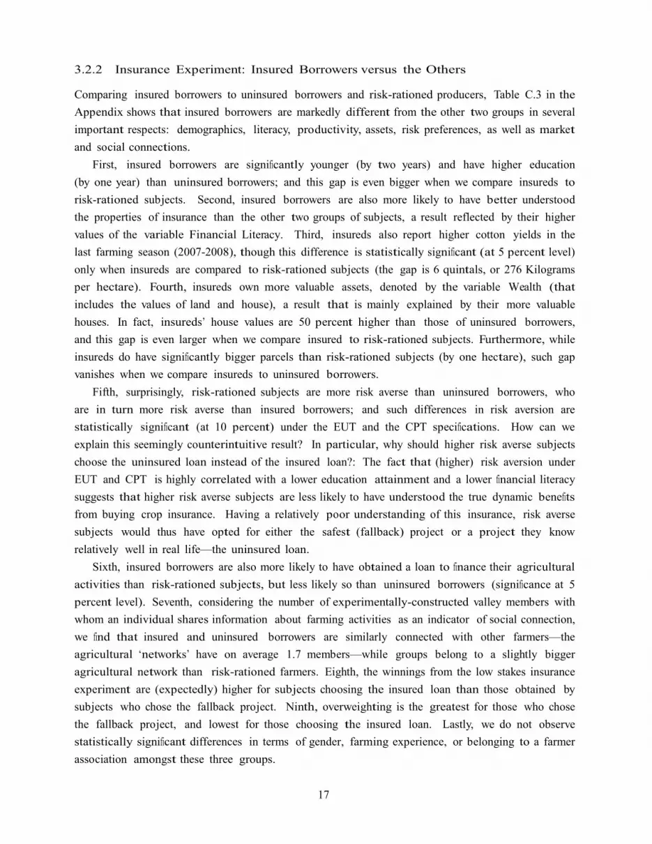
3.2.2 Insurance Experiment: Insured Borrowers versus the Others

Comparing insured borrowers to uninsured borrowers and risk-rationed producers, Table C.3 in the

Appendix shows that insured borrowers are markedly different from the other two groups in several

important respects: demographics, literacy, productivity, assets, risk preferences, as well as market

and social connections.

First, insured borrowers are significantly younger (by two years) and have higher education

(by one year) than uninsured borrowers; and this gap is even bigger when we compare insureds to

risk-rationed subjects. Second, insured borrowers are also more likely to have better understood

the properties of insurance than the other two groups of subjects, a result reflected by their higher

values of the variable Financial Literacy. Third, insureds also report higher cotton yields in the

last farming season (2007-2008), though this difference is statistically significant (at 5 percent level)

only when insureds are compared to risk-rationed subjects (the gap is 6 quintals, or 276 Kilograms

per hectare). Fourth, insureds own more valuable assets, denoted by the variable Wealth (that

includes the values of land and house), a result that is mainly explained by their more valuable

houses. In fact, insureds’ house values are 50 percent higher than those of uninsured borrowers,

and this gap is even larger when we compare insured to risk-rationed subjects. Furthermore, while

insureds do have significantly bigger parcels than risk-rationed subjects (by one hectare), such gap

vanishes when we compare insureds to uninsured borrowers.

Fifth, surprisingly, risk-rationed subjects are more risk averse than uninsured borrowers, who

are in turn more risk averse than insured borrowers; and such differences in risk aversion are

statistically significant (at 10 percent) under the EUT and the CPT specifications. How can we

explain this seemingly counterintuitive result? In particular, why should higher risk averse subjects

choose the uninsured loan instead of the insured loan?: The fact that (higher) risk aversion under

EUT and CPT is highly correlated with a lower education attainment and a lower financial literacy

suggests that higher risk averse subjects are less likely to have understood the true dynamic benefits

from buying crop insurance. Having a relatively poor understanding of this insurance, risk averse

subjects would thus have opted for either the safest (fallback) project or a project they know

relatively well in real life—the uninsured loan.

Sixth, insured borrowers are also more likely to have obtained a loan to finance their agricultural

activities than risk-rationed subjects, but less likely so than uninsured borrowers (significance at 5

percent level). Seventh, considering the number of experimentally-constructed valley members with

whom an individual shares information about farming activities as an indicator of social connection,

we find that insured and uninsured borrowers are similarly connected with other farmers—the

agricultural ‘networks’ have on average 1.7 members—while groups belong to a slightly bigger

agricultural network than risk-rationed farmers. Eighth, the winnings from the low stakes insurance

experiment are (expectedly) higher for subjects choosing the insured loan than those obtained by

subjects who chose the fallback project. Ninth, overweighting is the greatest for those who chose

the fallback project, and lowest for those choosing the insured loan. Lastly, we do not observe

statistically significant differences in terms of gender, farming experience, or belonging to a farmer

association amongst these three groups.

17

i

To sum up then, we saw that financial literacy, wealth, risk preferences, and social network

variables are likely to be correlated with the project choices made in the insurance experiment,

and we will include those variables in the regression analysis. We discuss in the next section

the econometric methods used in the estimation of those project choice decisions and the main

estimation results.

4 Econometric Specification We estimate ordered probit models, using the choices made in the final unconstrained round. The

base ordering is given by risk considerations: as risk aversion increases, one should expect to see

subjects switching from the uninsured loan (riskiest) to the insured loan, and then to the fallback

project (safest): A→C→B. Thus, in our base econometric specification, the dependent variable,

yi, which denotes the project choice by individual i, will take the value of 1, if the uninsured loan

project was chosen; 2, if it was the insured loan project; and 3, if it was the fallback project.

Using the latent utility framework, we define y * as an unobserved measure of utility for indi-

vidual i:32

y*i = X’iβ + εi (4)

where εi will be assumed to follow a logistic distribution, and X is the vector of regressors. Thus,

for our three-category ordered model we have that,

yi = j if αj-1 < y

*i ≤ αj, j=1,2,3 (5)

with α0 = -∞ and α3 = ∞; where the α ’

s indicate the cut points or thresholds that define the

project choice. Using the previous two equations, the probability of choosing project j can be

expressed as follows:

Pr (yi = j) = Pr (αj-1 < y*i ≤ αj) (6)

= Pr (αj-1 - X’iβ < εi ≤ αj - X’iβ)

= F (αj - X’iβ) – F (αj-1 - X’iβ),

where F (.) is the cumulative probability distribution of εi. The parameter vector and the cutpoint

parameters result from maximizing the following log-likelihood function:

ln L(α,β | X) = ΣNi=1Σ

Ni=1 ln[F (αj - X’iβ) – F (αj-1 - X’iβ)]

yi,j (7)

where yi,1 ; yi,2 ; yi,3 are three indicator variables with yi,j = 1 if yi = j; and yi,j = 0, otherwise.

The interpretation of the regression coeficients is as follows: Since the project choice used as a

dependent variable decreases with risk (a higher value is associated with choosing a safer project),

3 2 I am drawing on Cameron and Trivedi (2009) for this part.

18

a positive coeficient βi would indicate a higher probability of choosing a safer project. We run

ordered probit regressions with the standard errors clustered by the experimentally-constructed-

valleys, in order to correct for a possible intra-cluster correlation. We also include session fixed

effects in the regressions, in order to control for intra-session correlated decisions. The next section

discusses the estimation results.

4.1 Empirical Analysis

In this section we examine the main determinants of project choice in the high stakes insurance

experiment. In particular, we analyze the main predictors of choosing the riskiest project (uninsured

loan) instead of any of the other two safer projects (insured loan or fallback project). We will discuss

the effects of wealth, financial literacy, social connections, and variables constructed from within

the experiments (choices in the baseline experiment, winnings in the low stakes rounds, experiment

effects, and risk aversion).

The base specification includes the following independent variables: the level of assets, a vari-

able measuring the degree of social connection existing in the experimentally-constructed valleys,

the predicted choices made in the Baseline Experiment, low-stakes winnings in the Insurance Ex-

periment, and a variable that controls for the potential existence of a source of judgment bias called

“hot-hand” effect, which may arise from an attempt to discover trends in past information, and

results in an overestimation of the autocorrelation in the series of good or bad events

Our variable Wealth includes the value of land and house, while our social connection variable—

Agricultural Network — indicates the number of subjects in a given randomly-formed valley with

whom a person shares information about farming activities.33 This variable also controls for po-

tentially correlated decisions within each experimental valley.34 On the other hand, the variable

that predicts choices made in the baseline experiment—Risk Rationed — indicates the probability

of choosing the fallback project in that experiment,35 and intends to account for the potential

correlation between choices in the insurance experiment and those in the baseline experiment. The

variable Prior Rounds Earnings, which measures the winnings in Soles from the low stakes rounds

in the insurance experiment, controls for “wealth" effects that could have arisen if project choices

depended on how much winnings they earned in the prior rounds of the insurance experiment.

Finally, we control for the potential existence of a source of judgment bias called “hot-hand”

effect, which may arise from an attempt to discover trends in past information and results in an

overestimation of the autocorrelation in the series of good or bad events.36 Focusing solely on

negative events, this bias would imply that, for instance, drawing two consecutive black chips

3 3 Including demographic indicators would not change the results significantly. 3 4 While it could have been interesting to capture the way information is aggregated within different valleys and

how it is then translated into decisions under risk, by simply including the size of the agricultural network, we expect

to control for the influence that the members within a valley may have had on each individual’s pro ject choices. 3 5 We estimated a Probit regression of the unconstrained final high stakes round in the baseline game on age (in

years), education (years), gender, and owned land size (in hectares). 3 6 Offerman and Sonnemans (2004) report some evidence of the overrreaction resulting from hot-hand effects

in sports and financial markets. They further desing an experiment to distinguigh between hot-hand and

recency effects, the latter being the bias towards overweighting recent information and underweighting prior beliefs.

19

(which means that a very low average yield was drawn in a particular farming season) may lead

subjects to erroneously think that those events are autocorrelated and would then drive them to

rely on a safe project (i.e., either the fallback or the insured loan projects). This overreaction notion

is closely related to the overweighting of probabilities information, in the sense that the probability

of a bad recent event is overvalued, thus resulting in a too optimistic or too pessimistic behavior.

To control for this “hot-hand”effect, we use a dummy variable for drawing two consecutive

black chips in the last two low stakes rounds of the Insurance Experiment, and we expect a positive

(negative) correlation with the safer projects (insured loan or fallback project) take-up if there is an

overestimation (underestimation) of the autocorrelation in the series of black chips: once two black

chips are drawn, those subjects overestimating (underestimating) such autocorrelation would (not)

expect another black chip to be drawn in the next rounds, thus judging the insured loan or the

fallback project—choices which eliminate the chances of a loan default if a black chip is

drawn—more (less) attractive than the uninsured loan.

In addition to those controls, we are particularly interested in examining the effect that risk

preferences, education, and financial literacy can have over the project selection in the Insurance

Experiment. Our risk variable was estimated from a Holt-Laury (2002) type of binary lottery

experiment in which the same sample of subjects chose between a relatively safe lottery and a

relatively risky lottery along ten decision rows. Prizes are held constant in each row, while the

probability of the higher prize in each lottery decreases as the experiment progresses. The idea of

this design is that, unless subjects are extremely risk loving, they should start choosing the safe

lottery and switch to the risky lottery before or in the 10th row, where the prize from the risky

lottery is for sure greater than that from the safe lottery. Lottery choices were used to estimate

risk preferences by maximum likelihood. Results from that experiment are reported in Galarza

(2009). In the risk regression, higher education appears significantly correlated with lower risk

aversion. On the other hand, our Financial Literacy indicator intends to capture the level of

subjects’ comprehension about the main features of the insured and uninsured loan projects, and

takes values between 0 (meaning that subjects do not

know anything about the insured and uninsured loan projects) and 1 (meaning that subjects

know very well those projects).

Turning to the regression results shown in Table 5, in all four specifications considered, the

variables that enter with significant coeficients are the probability of being risk rationed, our

indicator of ‘hot-hand’ effect, and risk aversion. First, being risk rationed in the baseline experiment

makes subjects to be more likely to choose the safer projects in the insurance experiment as well.

This result should not be surprising and simply points to the consistency in choices across these

two types of experiments. Moreover, if one suspects that there is some endogeneity issues with the

inclusion of this variable, given that, after all, choices made by subjects in the baseline game may

be correlated with some other observable characteristics that also explain choices in the insurance

experiment, it should be mentioned that excluding this variable does not affect the qualitative

results under the four specifications considered.

Second, we find that subjects appear to underestimate the autocorrelation of very bad covariate

20

shocks, since once they face two consecutive black chips in their valleys they tend to choose the

risky project instead of the safer ones (presumably because they do not expect the next season to

face another black chip). This effect is significant (p-values < 0.06 in specifications [1], [2], & [3],

and p-value < 0.05 in specification [4]).

Third, interestingly, our risk estimate appears to have a quadratic, concave relationship with

project choices: higher risk aversion is positively correlated with a higher demand for safer projects,

but such relationship is decreasing. This non-linear relationship hints that the highest risk averse

subjects would prefer switching to the riskier project, a result that is rather puzzling. Taking

specification [1] alone (see column 2), we could explain this result noting that highly risk averse

subjects are more likely to have lower financial literacy (Spearman’s correlation coeficient of -0.26,

significant at 1 percent), and we could thus think that higher risk averse subjects, being less likely to

have understood the intertemporal and dynamic benefits of insurance, will have a lower demand for

it. However, when we control for financial literacy (specification [2] in column 2), the relationship

between risk aversion and project choice remains basically the same, meaning that financial literacy

does not explain project choices. It is rather surprising not to find that financial literacy affects

project choice (though its coeficient has a positive sign, meaning that higher financially literate

subjects are more prone to select the safer projects (in particular, the insured loan project), its

magnitude is negligible and statistically insignificant. We also tried to see if there was a non-linear

relationship, or if the individual components of this indicator were significant, but did not find any

evidence of it.

We further examined whether the interaction between financial literacy and risk aversion could

predict project choice (for some moderate degrees of risk aversion and financial literacy), but while

neither financial literacy nor its interaction term with risk aversion resulted statistically significant

(see specification [3] in column 4), and the standard errors of those variables become large. In

this case, risk aversion enters with a significant coeficient (at 10 percent), and its quadratic term

continues to be significant at 5 percent (p-value is 0.015). In all specifications where risk aversion

is included, its linear term and its quadratic expression are jointly statistically significant at either

the 10 percent (specification [3]) or 1 percent (specifications [1] & [2]).

Things are different when we include education (expressed in years) instead of financial literacy in

the regression, and we exclude the risk estimates (we did so because the estimation of the risk

preferences included dummy variables of education—illiterate, some primary, and some post-

secondary education—and including both education and risk would confound the effect of education

on project choice). Results in this case, reported in column (5), indicate that higher levels of

education are strongly correlated with a higher propensity to stay away from the risky, uninsured

loan project. The qualitative results in terms of the other regressors remain unchanged with respect

to specifications [1] & [2].

21

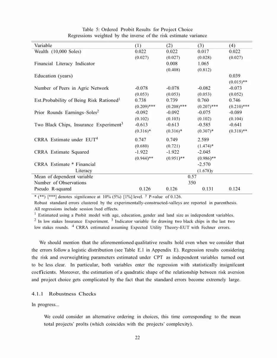
Table 5: Ordered Probit Results for Project Choice

Regressions weighted by the inverse of the risk estimate variance

Variable (1) (2) (3) (4) Wealth (10,000 Soles) 0.022 0.022 0.017 0.022

(0.027) (0.027) (0.028) (0.027) Financial Literacy Indicator 0.008 1.065

(0.408) (0.812) Education (years) 0.039

(0.015)** Number of Peers in Agric Network -0.078 -0.078 -0.082 -0.073

(0.053) (0.053) (0.053) (0.052) Est.Probability of Being Risk Rationed1 0.738 0.739 0.760 0.746

Prior Rounds Earnings–Soles2 (0.209)***

-0.092 (0.208)***

-0.092 (0.207)***

-0.075 (0.210)***

-0.089

Two Black Chips, Insurance Experiment3 (0.102)

-0.613 (0.103)

-0.613 (0.102)

-0.585 (0.104)

-0.641

(0.316)* (0.316)* (0.307)* (0.318)**

CRRA Estimate under EUT4 0.747 0.749 2.589

(0.680) (0.721) (1.474)* CRRA Estimate Squared -1.922 -1.922 -2.045

(0.944)** (0.951)** (0.986)** CRRA Estimate * Financial -2.570

Literacy (1.678)y

Mean of dependent variable 0.57

Number of Observations 350

Pseudo R-squared 0.126 0.126 0.131 0.124

* (**) [***] denotes significance at 10% (5%) [1%] level. y P-value of 0.126.

Robust standard errors clustered by the experimentally-constructed-valleys are reported in parenthesis.

All regressions include session fixed effects. 1 Estimated using a Probit model with age, education, gender and land size as independent variables. 2 In low stakes Insurance Experiment. 3 Indicator variable for drawing two black chips in the last two

low stakes rounds. 4 CRRA estimated assuming Expected Utility Theory-EUT with Fechner errors.

We should mention that the aforementioned qualitative results hold even when we consider that

the errors follow a logistic distribution (see Table E.1 in Appendix E). Regression results considering

the risk and overweighting parameters estimated under CPT as independent variables turned out

to be less clear. In particular, both variables enter the regression with statistically insignificant

coeficients. Moreover, the estimation of a quadratic shape of the relationship between risk aversion

and project choice gets complicated by the fact that the standard errors become extremely large.

4.1.1 Robustness Checks

In progress...

We could consider an alternative ordering in choices, this time corresponding to the mean

total projects’ profits (which coincides with the projects’ complexity).

22

– Not yet done.

Non-linear relationship with the financial literacy variable (get 3 quantiles of the density, and

include dummy variables for the lowest two)

– Result: Financial literacy is still insignificant, and results are basically the same.

Non-linear relationship with the risk preferences estimate (get 3 quantiles of the density, and

include dummy variables for the lowest two)

– Result: Same as using quadratic shape.

Only including the subsample of those who did not switch back and forth in the risk experi-

ment.

– Result: Quadratic shape is not significant, financial literacy becomes significant (at 5%),

wealth (1%), still significant hot-hand effect.

Excluding those who mistakenly chose the safe lottery in the 10th row of the risk experiment.

– Result: Quadratic shape is not significant, hot hand effect is significant and prob. of

being risk rationed becomes significant (at 5%).

Excluding those subjects who chose {project A, project B} & {project B, project A} (switched

from safe/loan [baseline experiment] to loan/safe [in insurance experiment], see Table 4).

– Result: It only makes risk estimates more significant (and wealth becomes significant).

5 (Preliminary) Conclusion In a context of collateral-constrained formal credit markets, the introduction of insurance is ex-

pected to help enhance the demand for credit by reducing the fear of losing collateral that prevents

potential borrowers from taking loans. This paper provides experimental evidence of such desired

credit crowding-in effect of insurance from Peru. Framing our experiments to recreate a similar

environment to the choices and outcomes that farmers have in real life, we started with a Baseline

Experiment where subjects had to choose between a fallback (safe) production project or produce

using an uninsured working capital loan (risky project). We then introduced a third project—

producing cotton with an insured loan—which allows us to measure the effect of insurance on

the demand for loans (Insurance Experiment). Our results show that while about a quarter of

our subjects are risk rationed, meaning that they chose to do the fallback project in the baseline

experiment, about 60 percent of those subjects switched to the insured loan project when it was

available.

Overall, in the Insurance Experiment, more than 50 percent of the subjects chose the insured

loan during the high stakes rounds. Given that this insurance contract eliminates by construction

23

the chance of loan default, this demand is likely to reflect the fear of losing collateral when one is

unable to repay a loan. While one could suspect that this very high insurance take-up rate may

simply reflect subjects’ desire to “try that new product" out of curiosity, there are two reasons

to believe that this was not the case. First, the insured loan take-up does not vary much even

during the low stakes rounds. Second, and more interestingly, using contingent valuation questions

in the post-experiment survey, we verify that indeed about 55 percent of farmers indicated that

they would be willing to buy the insured loan contract with the premium of 150 Soles per hectare.

The econometric results of the main predictors of project choice show that, controlling for wealth

and choices in the baseline experiment, project choice is affected by a ‘hot-hand’ effect that stem

from an underestimation in the autocorrelation in the sequence of very bad years (or black chips),

while the relationship with risk aversion appears to have a quadratic shape. That is, only low and

moderately risk averse subjects will choose the safest projects (i.e., fallback or insured loan), while

highly risk averse farmers will more likely choose the risky, uninsured loan project. Although there

is certainly more work to do in order to fully understand this result, this preliminary evidence

should be taken as suggestive of the usefulness of exploring some departures from the standard

microeconomic theory.

This paper contributes to the existing literature about the use of behavioral field experiments to

predict financial decisions made in a risky environment. A novel feature of our experimental design is

that it involves choices over alternative projects related to agricultural production decisions,

whose profits depend on the realizations of two random shocks: one intended to show the effects of

covariate, systemic variables, and the other, the effects of idiosyncratic factors. Another possible

use of our experimental design is in the education of potential beneficiaries of virtually any new

financial product.

24

References

[1] Banerjee, Abhijit and Esther Duflo (2008). “The Experimental Approach to Development

Economics," Working Paper, Massachusetts Institute of technology, Department of Economics

and Abdul Latif Jameel Poverty Action Lab.

[2] Becker, Gordon M., Morris H. DeGroot and Jacob Marschak (1964). “Measuring Utility by a

Single-Response Sequential Method," Behavioral Science, 9: 226-232.

[3] Boucher, Steve, Michael R. Carter and Catherine Guirkinger (2008). “Risk Rationing and

Wealth Effects in Credit Markets,” American Journal of Agricultural Economics, 90(2): 409-

423.

[4] Cameron, Colin and Pravin Trivedi (2009). Microeconometrics using Stata. Texas: Stata Press.

[5] Cardenas, Juan Camilo and Jeffrey Carpenter (2005). “Experiments and Economic Develop-

ment: Lessons from field labs in the developing world," Working Paper.

[6] Carter, Michael R. and Christopher Barrett (2006). “The Economics of Poverty Traps and

Persistent Poverty: An Asset-based Approach,” Journal of Development Studies, 42(2): 178-

199.

[7] Cole, Shawn, Xavier Giné, Jeremy Tobacman, Petra Topalova, Robert Townsend, and James

Vickery (2008). “Barries to Household Risk Management: Evidence from India," Working

Paper.

[8] Davis, Douglas and Charles Holt (1993). Experimental Economics. Princeton, NJ: Princeton

University Press.

[9] Dercon, Stefan (2005). “Risk, Insurance, and Poverty: A Review." In: Dercon, Stefan (ed.),

Insurance Against Poverty. Oxford, New York: Oxford University Press.

[10] Feder, Gershon (1980). “Farm Size, Risk Aversion and the Adoption of New Technologies

under Uncertainty," Oxford Economic Papers, 32(2): 263-283.

[11] Fox, Craig R. and Russel A. Poldrack (2009). “Prospect Theory and the Brain," In: Glimcher,

Paul W., Colin F. Camerer, Ernst Fehr and Russell A. Poldrack (eds.), Neuroeconomics.

Decision Making and the Brain (pp.145-173). London; San Diego, CA: Academic Press.

[12] Galarza, Francisco (2009). “Choices under Risk in Rural Peru," AAE Staff Paper # 542,

University of Wisconsin-Madison, Department of Agricultural and Applied Economics (AAE).

[13] Giné, Xavier, Pamela Jakiela, Dean Karlan and Jonathan Morduch (2009). “Microfinance

games," Working Paper.

[14] Giné, Xavier, Robert Townsend and James Vickery (2008). “Patterns of Rainfall Insurance

Participation in Rural India," World Bank Economic Review, forthcoming.

[15] Giné, Xavier and Dean Yang (2010). “Insurance, Credit, and Technology Adoption: Field

Experimental Evidence from Malawi," Journal of Development Economics, 89(1): 1-11.

[16] Harrison, Glenn and John List (2004). “Field Experiments," Journal of Economic Literature,

42(4): 1013-1059.

25

[17] Levy, Haim and Moshe Levy (2002). “Arrow-Pratt Risk Aversion, Risk Premium and Decision

Weights," Journal of Risk and Uncertainty, 25(3): 265-290.

[18] Lybbert, Travis J. (2006). “Indian Farmer’s Valuation of Yield Distributions: Will Poor Farm-

ers Value ‘Pro-Poor’ Seeds?," Food Policy, 31(5): 415-441.

[19] Miranda, Mario (1991). “Area Crop Yield Insurance Reconsidered,” American Journal of Agri-

cultural Economics, 83(3): 650-665.

[20] Morduch, Jonathan (1995). “Income Smoothing and Consumption Smoothing," Journal of

Economic Perspectives, 9(3): 103-114.

[21] Offerman, Theo and Joep Sonnemans (2004). “What’s Causing Overreaction? An Experimen-

tal Investigation of Recency and the Hot-hand Effect," Scandinavian Journal of Economics,

106(3): 533-553.

[22] Tversky, Amos and Daniel Kahneman (1992). “Advances in Prospect Theory: Cumulative

Representations of Uncertainty,” Journal of Risk and Uncertainty, 5(4): 297-323.

26

Appendix A. Information Shared with Subjects

1. Number and color of chips by type of valley-wide average yields (VAYs): black, red, white,

blue, green

2. Historical valley-wide average cotton yields: 1986-2006 (bar graph)

3. Project A (cotton with loan) payoffs for the normal individual luck (luck dimension not

shown) by type of VAY

4. Example of calculating the payoffs for the normal individual luck (luck dimension not shown)

with normal VAY

5. Number and color of balls by type of individual luck: purple, white, yellow

6. Project A’s payoffs (by type of luck and category of VAY)

7. Project B’s payoffs (by type of luck and category of VAY)

8. Project A’s and B’s payoffs (by type of luck and category of VAY) on the same page

9. Project C’s payoffs (by type of luck and category of VAY)

10. Project A’s, B’s & C’s payoffs (by type of luck and category of VAY) on the same page

{End of Farming experiments}

11. Maximum and minimum prizes of lotteries

12. Lotteries’ payoffs for decision row 2

13. Lotteries’ payoffs for decision row 8 (symmetric to 2)

14. Lotteries’ payoffs for decision rows 2 and 8 (together)

15. Practice experiment sheet for binary lottery experiment (ten decision rows)

16. Experiment sheet for high-stake binary lottery experiment (ten decision rows)

{End of Lottery Experiment}

27

Appendix B. Summary of Experimental Procedures

The following is the structure of the farming experiments conducted in Pisco.

Entry survey

Introduction of the experimental session

Presentation of the experiment: goals

Description of project A: cotton with loan

– Description of Covariate shock: valley-wide average yield (VAY), slide

Examples of how different colored chips represent distinct types of VAY

Example of how different colored chips imply different profits, slide

Example of how the payoff for the normal VAY was calculated, slide

– Description of Idiosyncratic shock: individual luck, slide

Example of how different colored balls (and different colored chips) imply

different profits for project A (uninsured loan)

– Example of drawing a valley chip and an individual luck (see profits), slide

Description of project B: cotton without loan (fallback), slide

– Example of drawing a valley chip and an individual luck (see profits)

Comparison of outcomes in projects A and B, slide

– Example of drawing a valley chip and an individual luck (compare profits if project were

chosen A versus profits if project B were chosen)

Play six rounds of low stakes, baseline experiment (A versus B)

– Payments are calculated and shown to subjects

Play six rounds of high stakes, baseline experiment (A versus B)

– Payments are calculated and shown to subjects

Description of project C: cotton with loan and index insurance, slide

– A salient feature: no default loans under any covariate shock or idiosyncratic shock

– Example of drawing a valley chip and an individual luck (see profits)

Comparison of outcomes in projects A, B, and C, slide

– Example of drawing a valley chip and an individual luck (compare profits if project were

chosen A versus profits if projects B or C were chosen)

Play six rounds of low stakes, insurance experiment (A versus B versus C)

28

– Payments are calculated and shown to subjects

Play six rounds of high stakes, insurance experiment (A versus B versus C)

– Payments are calculated and shown to subjects

End of Farming Experiments

29

Appendix C. Tables

Table C.1 Summary Statistics

Variable Mean Std. Dev. N Dependent variable Insured loan take-up rate (high stakes) 0.57 0.49 378 Demographics and Education Age (years) 54.9 13.3 367 Aged less than 40 0.14 0.35 367 Aged between than 40 and 50 0.19 0.39 367 Aged between than 50 and 60 0.33 0.47 367 Aged over 60 0.33 0.47 367 Female (Yes=1) 0.27 0.44 367 Education (years) 6.33 4.11 365 Illiterate 0.05 0.23 365 Some primary school 0.51 0.50 365 Some secondary school 0.34 0.47 365 Completed higher than secondary school 0.09 0.29 365 Financial literacy indicator1 0.54 0.20 378 Agriculture and Assets Farming experience (years) 23.9 12.7 368 Size of owned agricultural plot (hectares) 6.03 5.57 367 Size of sown land (hectares)2 5.01 4.13 365 Cotton yields (quintals per hectare)2 46.8 14.8 293 Self-reported value of owned ag plot (000 Soles) 7.43 8.78 307 Self-reported value of house (000 Soles) 15.92 21.0 321 Self-reported value of assets (000 Soles)3 20.42 21.8 362 Networks, Credit, and Insurance Talked to somebody in her “valley" about farming(Yes=1) 0.67 0.47 378 Number of “valley" members in her agricultural network 1.73 1.61 378 Has ever been a local authority (Yes=1) 0.39 0.49 365 Belongs to a farmer association (Yes=1) 0.29 0.46 364 Got credit for farming activities (Yes=1)2 0.61 0.49 378 Got formal credit (Yes=1) 0.38 0.49 232 Got credit from cotton mills (Yes=1) 0.28 0.45 232

Has life insurance (Yes=1) 0.14 0.37 367 Has Accident insurance (Yes=1) 0.10 0.30 367 Experimental Variables Risk rationed (Baseline Experiment) (Yes=1) 0.24 0.43 378 Risk parameter estimate, EUT4 0.45 0.29 365 Risk parameter estimate, CPT4 0.74 0.32 365 Probability weighting parameter estimate, CPT5 0.54 0.21 365 Overweighting small probabilities (Yes=1), CPT5 0.80 0.40 365 Drew two black chips,last low-stake rounds Insurance Experiment 0.02 0.13 378 Winnings from low stakes Insurance Experiment (Soles) 3.04 0.85 378 1 Indicator calculated using knowledge of insurance and loan project, as well as a self-reported degree of

comprehension. 2 It refers to the 2007-2008 farming season. 3 Wealth includes the values of land & house. 4 EUT (CPT): Risk estimate assuming Expected Utility Theory (Cumulative Prospect Theory). 5 Overweighting means that the probability weighting parameter is less than or equal to 0.7.

30

Table C.2: Summary Statistics by Project Choice in Final Unconstrained Round

Baseline Experiment

Name Uninsured Loan (A) Fallback (B) T-Test

Mean S.D. N Mean S.D. N (A)=(B)

Demographics and Education Age (years) 54.6 0.80 278 55.9 1.39 89 -0.80 Young (age < 40) 0.14 0.02 279 0.12 0.04 89 0.48 Middle (age: [50-60]) 0.34 0.03 279 0.33 0.05 89 0.19 Old (age > 60) 0.33 0.03 279 0.36 0.05 89 -0.57 Female 0.24 0.03 279 0.36 0.05 89 -2.15** Education (years) 6.35 0.25 279 6.27 0.45 86 0.17 Illiterate 0.05 0.21 279 0.09 0.29 86 -1.37* Some primary school 0.51 0.50 279 0.50 0.50 86 0.20 Some secondary school 0.35 0.48 279 0.30 0.46 86 0.85 Higher than second. school 0.09 0.29 279 0.10 0.31 86 -0.40 Financial literacy indicator 0.55 0.20 286 0.51 0.20 92 1.49*

Agriculture and Assets

Farm experience (years) 23.4 12.6 279 25.4 13.1 89 -1.27 Size of owned land (Has) 6.28 0.36 278 5.24 4.17 89 1.85** Size of sown land (Has)1 5.23 4.15 277 4.32 4.02 88 1.83** Cotton yields (QQ/ Ha.)1 47.4 14.4 230 44.8 16.2 63 1.12 Land value (000 Soles) 7.64 9.39 235 6.76 6.42 72 0.91 House value (000 Soles) 15.44 19.65 241 17.35 24.32 80 -0.63 Wealth (000 Soles) 20.14 20.84 274 21.30 24.83 88 -0.40

Networks and Credit

Belongs to ag network 0.71 0.45 287 0.56 0.50 91 2.56*** # members in ag network 1.82 1.60 287 1.44 1.62 91 1.97** Has been local authority 0.40 0.49 277 0.35 0.48 88 0.88 Belongs to farm association 0.27 0.45 277 0.36 0.48 87 -1.47* Got credit for farming activities 0.66 0.48 286 0.48 0.50 92 3.01*** Got formal credit 0.36 0.48 188 0.50 0.51 44 -1.71** Got credit from a cotton mill 0.31 0.46 188 0.14 0.35 44 2.76***

Experimental Outcomes

Risk estimate under EUT2

0.44

0.30

280

0.46

0.29

85

0.48 Risk estimate under CPT2 0.73 0.33 280 0.77 0.31 85 0.92 Prob. weighting parameter est., CPT 0.54 0.21 280 0.52 0.20 85 0.81 Overweighting small probabilities, CPT3 0.78 0.42 280 0.87 0.34 85 -1.86** Drew two black chips, low-stake rounds4 0.02 0.13 287 0.01 0.10 91 0.43 Winnings, low stakes Insurance Experiment5 3.07 0.88 287 2.96 0.73 91 1.07 ( ) [ ]: Significant at 10% (5%) [1%] level. T-test assumes unequal variances. 1 It refers to the 2007-2008 farming season. 2 EUT (CPT): Risk estimate assuming Expected Utility Theory (Cumulative Prospect Theory). 3 Overweighting means that the probability weighting parameter under CPT is less than or equal to 0.7. 4 In last two low-stake rounds of Insurance Experiment. 5 Expressed in Soles.

31

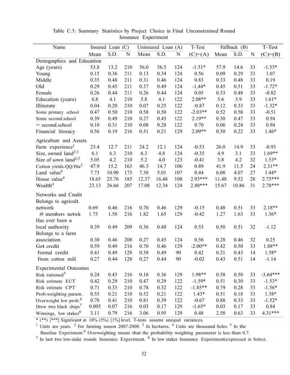
Table C.3: Summary Statistics by Project Choice in Final Unconstrained Round

Insurance Experiment

Name Insured Loan (C) Uninsured Loan (A) T-Test Fallback (B) T-Test

Mean S.D. N Mean S.D. N (C)=(A) Mean S.D. N (C)=(B) Demographics and Education Age (years) 53.8 13.2 210 56.0 56.5 124 -1.51* 57.9 14.6 33 -1.53* Young 0.15 0.36 211 0.13 0.34 124 0.56 0.09 0.29 33 1.07 Middle 0.35 0.48 211 0.31 0.46 124 0.83 0.33 0.48 33 0.19 Old 0.29 0.45 211 0.37 0.49 124 -1.44* 0.45 0.51 33 -1.72* Female 0.26 0.44 211 0.26 0.44 124 0.05 0.33 0.48 33 -0.82 Education (years) 6.8 4.1 210 5.8 4.1 122 2.08** 5.6 3.9 33 1.61* Illiterate 0.04 0.20 210 0.07 0.25 122 -0.87 0.12 0.33 33 -1.32* Some primary school 0.47 0.50 210 0.58 0.50 122 -2.03** 0.52 0.50 33 -0.51 Some second.school 0.39 0.49 210 0.27 0.45 122 2.19** 0.30 0.47 33 0.94 > second.school 0.10 0.31 210 0.08 0.28 122 0.70 0.06 0.24 33 0.94 Financial literacy 0.56 0.19 216 0.51 0.21 129 2.09** 0.50 0.22 33 1.46*

Agriculture and Assets

Farm experience1 23.4 12.7 211 24.2 12.1 124 -0.53 26.0 14.9 33 -0.93 Size, owned land2;3 6.1 6.3 210 6.3 4.8 124 -0.35 4.9 3.1 33 1.69** Size of sown land2;3 5.05 4.2 210 5.2 4.0 123 -0.41 3.8 4.2 32 1.53* Cotton yields-QQ/Ha2 47.9 15.2 163 46.3 14.7 106 0.89 41.9 11.5 24 2.31** Land value4 7.73 10.90 173 7.30 5.01 107 0.44 6.08 4.07 27 1.44* House value4 18.65 25.76 185 12.37 16.48 108 2.93*** 11.48 9.52 28 2.75*** Wealth4 23.13 26.66 207 17.08 12.34 124 2.80*** 15.67 10.86 31 2.78***

Networks and Credit

Belongs to agricult. network 0.69 0.46 216 0.70 0.46 129 -0.15 0.48 0.51 33 2.18** # members netwk 1.75 1.58 216 1.82 1.65 129 -0.42 1.27 1.63 33 1.56*

Has ever been a local authority 0.39 0.49 209 0.36 0.48 124 0.53 0.50 0.51 32 -1.12 Belongs to a farm association 0.30 0.46 208 0.27 0.45 124 0.56 0.28 0.46 32 0.25 Got credit 0.59 0.49 216 0.70 0.46 129 -2.00** 0.42 0.50 33 1.88** Formal credit 0.41 0.49 128 0.38 0.49 90 0.42 0.21 0.43 14 1.58* From cotton mill 0.27 0.44 128 0.27 0.44 90 -0.02 0.43 0.51 14 -1.14

Experimental Outcomes

Risk rationed5 0.24 0.43 216 0.16 0.36 129 1.98** 0.58 0.50 33 -3.64*** Risk estimate EUT 0.42 0.29 210 0.47 0.29 122 -1.59* 0.51 0.30 33 -1.53* Risk estimate CPT 0.71 0.33 210 0.78 0.32 122 -1.85** 0.79 0.28 33 -1.56* Prob.weighting param. 0.55 0.21 210 0.52 0.21 122 1.43* 0.51 0.18 33 1.38* Overweight low prob.6 0.78 0.41 210 0.81 0.39 122 -0.67 0.88 0.33 33 -1.52* Drew two black chips7 0.005 0.07 216 0.03 0.17 129 -1.65* 0.03 0.17 33 0.84

Winnings, low stakes8 3.11 0.79 216 3.06 0.95 129 0.48 2.58 0.63 33 4.31***

* (**) [***] Significant at 10% (5%) [1%] level. T-tests assume unequal variances. 1 Units are years. 2 For farming season 2007-2008. 3 In hectares. 4 Units are thousand Soles. 5 In the

Baseline Experiment.6 Overweighting means that the probability weighting parameter is less than 0.7. 7 In last two low-stake rounds Insurance Experiment. 8 In low stakes Insurance Experiment(expressed in Soles).

32

From whom did

you receive the TA

or T?

>> Table 1

The TA or T

was?

>> Table 2

TA 1 TA 2 T 1 T 2

Appendix D. Surveys Conducted

D.1 Entry Survey

I. General Information

1. Name

2. Gender

3. What is your age?

4. How many children younger than 15 years of age currently live in your household?

5. How many completed years of education do you have?

6. The person with the most education in your household, how many completed years of education

does he or she have?

7. How many years have you dedicated to agricultural activities?

8. How many hectares does your household own?

9. How many hectares did you work in the past year?

10. How much do you think you would have to pay to rent a hectare of land with similar charac-

teristics to those of your principal cotton parcel?

Row by

row,

mark

with an

X the

space

that

correspo

nds to

the subject’s

answer.

11.1 Did

you

plant

cotton in

the

years

(fi )?

11.2

What

were

your

cotton

yields in

the

years

()?

(QQ x

Ha)

11.3

Do you believe that

your cotton yields in

the years () were () than

those of other farmers

in your neighborhood?

11.4. In the years (fi ), did youfi A.

Become

sick or

injured?

B.

Suffer any

kind of

theft?

(Seeds,

cotton,

pesticides,

etc.)

C.

Suffer a

problem

with the

climate?

D.

Suffer an

infestation

or blight

in your

cotton

crop?

E.

Have

problems

with the

irrigation

infrastructure

in your area?

ye

s N

o Highe

r Equal Less Yes No Yes No Yes No Yes No Yes No

2007•

2008

2006•

2007

2005•

2006

12. During the past 5 years, did you receive any type of technical assistance (TA) or training (T)

related to the production of cotton?

If no, continue to question 14. If yes, continue to 13.

13. Describe the last two TA or T that you received? Table 1

1. Cotton gin

2. Other private business

3. NGO

4. Ministry of Agriculture

5. Other? Who?

Table 2

1.Very beneficial

2. beneficial

3. Somewhat

beneficial

4. Not beneficial

33

II. Social Capital

14. Are you or have you ever been any kind of authority of some association, in your community,

or irrigation commission?

15. Do you currently belong to any association of farmers? III. Insurance

Row by row,

mark with an X

the space that

corresponds to

the subject’s

answer.

16.1

Do you

know

what ()

insurance

is?

yes, quest.

16.2

No, quest.

16.3

16.2

Do you have to pay

for (fi ) insurance?

16.3

Do you or

does anyone

in your

household

have (fi )

insurance?

yes, Q. 16.4

No, Q. 16.5

16.4

If so, does

this person

pay for the

(fi )

insurance?

16.5

Do you know

who delivers

the services of

() insurance?

16.6

Only if they

respond

YES to

question

16.1

Do you

know what

benefits you

receive from

(fi )

insurance?

(Table 3)

The public sector

The Caja rural or a ban

k

Insu

rance

compan

y

Do not know

Yes No Yes No Doesn

’t

know

Yes No Yes No

Health Accidents Life/burial/ funeral

Debt Other? Which? Table 3

1. Free or less expensive medical attention in case of an

accident

2. Gives my family money should I pass away.

3. Medical attention in a hospital

4. Pays my debts if I pass them to my next of kin

5. Pays for my burial and/or funeral,

17. Would you be interested in paying a monthly premium to an institution in exchange for receiving

a payment ONLY in the case that you:

Are ill or injured

Suffer an infestation or blight in your crops

Suffer a problem with the climate (e.g., drought)

Suffer problems with the irrigation infrastructure

D.2 Exit Survey

I. Networks

1. How many people in the group in which you are seated do you know?

2. How many people in the group have you spoken with about farming activities (e.g., what to

plant, input use, etc.)?

II. Assets

3. The house in which you live is

Owned by you Owned by your parents/in-laws Owned by others Rented

(if rented, continue to question 5)

4. How much do you think you would have to pay to buy a house similar to yours?

Amount Soles

5. Do you possess one of the following consumer goods?

34

tor

_Car or light truck _Motorcycle Heavy truck Trac-

III. Credit

6. If you applied for a loan at the local urban or rural Caja or a bank, do you think they would

give it to you?

7. If you applied for a loan at a cotton gin, do you think they would give it to you?

8. If you applied for a loan from an informal moneylender, do you think they would give it to you?

9. In the years 2007-2008, did you obtain a loan in order to pay for your costs of production?

(If no, continue to question 11)

10. From whom did you obtain this loan?

_Bank or Caja Cotton gin _Informal lender

IV. Agricultural Insurance

11. Do you think that the instructions we gave you today prior to today’s activities were:

Very dificult __Dificult Easy Very easy

12. Do you remember what happened if you obtained a loan without insurance and could not repay

the loan?

What happened?

13. The indemnification that the insurance paid you depended on the average yields in the valley?

14. Did it depend on individual luck?

15. If someone were to offer you insurance similar to what we saw in activity 1 for the next

agricultural year, would you be interested in buying it?

16. Would you be interested in paying XX Soles per hectare for insurance similar to what we saw

in activity 1 (i.e., farming experiments)? ( ) YES >> Mark with an X the

maximum he/she would be willing to pay ( ) NO >> Mark with an X the

maximum he/she would be willing to pay S/. XX+25 S/. XX•25 S/. XX+50 S/. XX•50 S/. XX+75 S/. XX•75 S/. XX+100 S/. XX•100 More less

XX was set at 100, and 150, and 200 Soles.

35

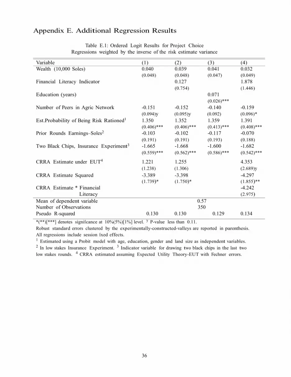
Appendix E. Additional Regression Results

Table E.1: Ordered Logit Results for Project Choice

Regressions weighted by the inverse of the risk estimate variance

Variable (1) (2) (3) (4) Wealth (10,000 Soles) 0.040 0.039 0.041 0.032

(0.048) (0.048) (0.047) (0.049) Financial Literacy Indicator 0.127 1.878

(0.754) (1.446) Education (years) 0.071

(0.026)*** Number of Peers in Agric Network -0.151 -0.152 -0.140 -0.159

(0.094)y (0.095)y (0.092) (0.096)*

Est.Probability of Being Risk Rationed1 1.350 1.352 1.359 1.391

(0.406)*** (0.406)*** (0.413)*** (0.408)*** Prior Rounds Earnings–Soles2 -0.103 -0.102 -0.117 -0.070

(0.191) (0.191) (0.193) (0.188) Two Black Chips, Insurance Experiment3 -1.665 -1.668 -1.600 -1.682

(0.559)*** (0.562)*** (0.586)*** (0.542)***

CRRA Estimate under EUT4 1.221 1.255 4.353 (1.238) (1.306) (2.689)y

CRRA Estimate Squared -3.389 -3.398 -4.297 (1.739)* (1.750)* (1.855)** CRRA Estimate * Financial -4.242

Literacy (2.975)

Mean of dependent variable 0.57 Number of Observations 350

Pseudo R-squared 0.130 0.130 0.129 0.134

*(**)[***] denotes significance at 10%(5%)[1%] level. y P-value less than 0.11.

Robust standard errors clustered by the experimentally-constructed-valleys are reported in parenthesis.

All regressions include session fixed effects. 1 Estimated using a Probit model with age, education, gender and land size as independent variables. 2 In low stakes Insurance Experiment. 3 Indicator variable for drawing two black chips in the last two

low stakes rounds. 4 CRRA estimated assuming Expected Utility Theory-EUT with Fechner errors.

36