Robust Adaptive Stabilization of Linear Time-Invariant Dynamic Systems by Using Fractional-Order Holds and Multirate Sampling Controls

Hindawi Publishing CorporationDiscrete Dynamics in Nature and SocietyVolume 2010, Article ID 620546, 27 pagesdoi:10.1155/2010/620546

Research ArticleRobust Adaptive Stabilization ofLinear Time-Invariant Dynamic Systems byUsing Fractional-Order Holds andMultirate Sampling Controls

S. Alonso-Quesada and M. De la Sen

Department of Electricity and Electronics, Faculty of Science and Technology,University of Basque Country, Leioa 48940, Spain

Correspondence should be addressed to S. Alonso-Quesada, [email protected]

Received 8 June 2009; Accepted 2 February 2010

Academic Editor: Francisco Solis

Copyright q 2010 S. Alonso-Quesada and M. De la Sen. This is an open access article distributedunder the Creative Commons Attribution License, which permits unrestricted use, distribution,and reproduction in any medium, provided the original work is properly cited.

This paper presents a strategy for designing a robust discrete-time adaptive controller forstabilizing linear time-invariant (LTI) continuous-time dynamic systems. Such systems may beunstable and noninversely stable in the worst case. A reduced-order model is considered to designthe adaptive controller. The control design is based on the discretization of the system with theuse of a multirate sampling device with fast-sampled control signal. A suitable on-line adaptationof the multirate gains guarantees the stability of the inverse of the discretized estimated model,which is used to parameterize the adaptive controller. A dead zone is included in the parametersestimation algorithm for robustness purposes under the presence of unmodeled dynamics in thecontrolled dynamic system. The adaptive controller guarantees the boundedness of the systemmeasured signal for all time. Some examples illustrate the efficacy of this control strategy.

1. Introduction

Adaptive control theory has been widely applied for stabilizing increasingly complexengineering systems with large uncertainties [1], including the incorporation of parallelmultiestimation and time-delayed and hybrid models [2–6]. Such model uncertainties maycome from the fact that the parameters of the dynamic system model are partially or fullyunknown and/or from the presence of unmodeled dynamics [3]. On the other hand, discreteequations are useful for modeling and controlling discretized continuous-time systems inpractical situations [2, 5–9] and as a tool for describing more complex nonlinear structures viadiscretization [10, 11]. A frequently used method to stabilize an unknown dynamic system is

2 Discrete Dynamics in Nature and Society

based on the model reference adaptive control (MRAC) problem [12]. However, the presenceof unstable system zeros does not make possible the design of a controller to achieve themodel-matching objective unless such unstable zeros are transmitted to the reference model[1, 2, 6, 13, 14]. Unfortunately, such a transmission cannot be available if some of the zerosof the system to be controlled are unknown as it can occur in the context of the adaptivecontrol where the dynamic system may be completely or partially unknown. However, thereare several alternative methods to circumvent this difficulty and carry out the stable adaptivecontrol design. Two of them depend on relaxing the control objective from the MRAC to theless exigent adaptive pole-placement control (APPC) [15, 16]. In this way, the stabilization ofthe feedback (or closed-loop) system can be ensured although its transient behavior cannotbe fixed to a predefined one. On one hand, the method in [15] includes a modification in theestimated parameters to ensure the controllability of the estimation model of the dynamicsystem. In this way, closed-loop unstable pole-zero cancellations are avoided, which is crucialfor the controller synthesis. Such a method is applicable for both continuous-time anddiscrete-time dynamic systems to be controlled. On the other hand, the research [16] may beused in the case of continuous-time dynamic systems. There, a periodic piecewise constant-gain controller is added in the feedback chain. In the nonadaptive case, the gain valuesare those required so that the discretized system model under the fundamental samplingperiod and a zero-order hold (ZOH) could be stabilized. It is worth that such a control gainis piecewise constant during the sampling period in order to place the discretized poles atstable desired locations. Concretely, each sampling period is split into a certain finite numberof uniform subintervals and the control gain takes a different value within each subinterval.In this way, the controller consists of a constant vector of gains. In this sense, the controllerworks with a sampling rate faster than that used to discretize the controlled system. In theadaptive case, the discretized dynamic system model parameters are on-line updated; thenthe controller gains vector is time varying and converges asymptotically to a constant one.

Another method, which does not relax the MRAC objective, to overcome the drawbackof the unstable zeros of a continuous-time dynamic system is the design of a discrete-timecontroller with the use of a hold device combined with a multirate sampling with fast inputrate in the discretization of the continuous-time system [7, 8]. In this way, an inversely stableestimated model of the discretized dynamic system can be obtained and a controller can bedesigned to match a stable arbitrarily chosen discrete-time reference model since all of thediscretized zeros may be cancelled if suited. In this context, this paper presents a robust adaptivecontrol scheme for stabilizing uncertain controlled continuous-time dynamic systems while matchinga freely chosen discrete-time reference model, with a bounded tracking-error, to be applied when thecontinuous-time system is unknown and subject to the presence of unmodeled dynamics. The mainnovelty is that the discrete zeros may be always stabilized even if the zeros of the continuoussystem are not all stable. As a result, the reference model zeros can all be freely fixed. Thecontrol scheme is based on the discretization process by combining the use of a fractional-order hold (FROH) and a multirate with fast sampling control signal. In this way, theestimated discretized model can be guaranteed to be inversely stable by means of a suitableon-line updating of the multirate gains without requirements neither on the stability of thecontinuous-time zeros nor the size of the sampling period [17]. Such a strategy gives place tohybrid systems where continuous-time and discrete-time dynamics are mixed. Concretely, adiscrete-time controller is designed to govern the behavior of a continuous-time dynamicalsystem. Epidemic control of infectious diseases and species population control systems inEcology are two typical examples of this class of hybrid systems [18–20]. A discrete-timecontrol strategy depending on a pulse vaccination is designed in [18]. Such vaccination pulses

Discrete Dynamics in Nature and Society 3

work as a discrete-time control signal and the eradication of the diseases is reached providedthat the vaccination rate is sufficiently large. The researches [19, 20] study, respectively, thenecessary conditions which guarantee the stabilization and permanence of single-speciesand predator-prey systems populations in their respective habitats. Both are continuous-time dynamic systems which can be described efficiently by means of discrete-time modelsin order to prescribe its evolution and then to develop discrete-time control strategies toensure the permanence of the species. All of these systems are subject to eventual changes inthe continuous-time dynamics whenever the discrete-time control action takes place. In thissense, they belong to a class of switched systems whose stability and stabilization conditionshave been studied in the recent literature [4, 21].

Furthermore, the presented control strategy guarantees the stabilization of thecontinuous-time dynamic system without any assumption about the stability of its zeros,which had been supposed in previous works [13, 22], and without requiring estimatesmodification in contrast with previous works on the subject [2, 15]. Such relaxationsconstitute the main contribution of the present work. A FROH is used since it allows abetter accommodation of discrete adaptive techniques to the transient response of discrete-time controlled continuous-time dynamic systems [9]. Furthermore, the estimation algorithmincludes a relative adaptation dead-zone to deal with the presence of unmodeled dynamics[14]. Such a dead-zone is crucial to ensure the estimates convergence and the stability of theadaptive control system. The stabilization is guaranteed provided that (1) the continuous-timedynamic system is stabilizable and observable (2) the size of the unmodeled dynamics is sufficientlysmall, and (3) such an unmodeled dynamics can be related to the system input by means of additiveand/or multiplicative stable transfer functions.

The paper is organized as follows. Section 2 presents the discretization process usedto obtain an inversely stable discretized dynamic system model from a possibly inverselyunstable continuous-time dynamic system. Section 3 deals with the control design to matcha discrete-time reference model at sampling instants for both nonadaptive and adaptivecases. Then, the stability analysis of the designed adaptive control algorithm is presentedin Section 4. Finally, simulation results, which illustrate the behavior of the adaptive controlsystem, are shown in Section 5 and conclusions end the paper in Section 6.

2. Problem Statement

Consider a linear time invariant SISO and strictly proper continuous-time dynamic systemdescribed by the following state-space equations:

x(t) = Ax(t) + Bu(t), y(t) = Cx(t), (2.1)

where u(t) and y(t) are, respectively, the control (or input) and measured (or output) signals,x(t) ∈ R

n is the state vector, and A, B, and C are constant matrices of suitable dimensions.The transfer function of (2.1) is Gp(s) = q(s)/p(s) = C(sIn −A)−1B where n = Deg(p(s)) ≥Deg(q(s)) = m, s denotes the Laplace transform argument [1], and In represents the n-orderidentity matrix. In the sequel, the controlled dynamic system is referred to as the “plant”to be controlled as it is commonly referred to in the Engineering Automation context. Thefollowing assumptions are made on the plant.


Assumption 1. (i) An upper-bound n of the plant order n is known as it is the nominal ordern0 ≤ n.

(ii) The plant realization matrices can be expressed as

A =

[A0 0

A21 A22

], B =

[B0

B21

], C =

[C0 C12

], (2.2)

where {A0, B0, C0} denotes the state-space realization for the nominal model of the plant andthe other matrix blocks are related to the unmodeled dynamics. In this context, the statevector is composed of two sets of state variables, namely, x �

[xT0 xT1

]T where x0 ∈ Rn0

is the nominal state vector. Furthermore, the eigenvalues of the block A22 are strictly stable,‖B21‖ ≤ μ0, and ‖C12‖ ≤ μ0 for some sufficiently small real μ0 > 0 with ‖M‖ denoting thenorm of the matrix M.

(iii) The nominal pair (A0, C0) is observable.

Remark 2.1. (i) Given any state-space realization, there always exists an infinite number ofstate-space realizations in triangular form as (2.2) which have the same transfer functionthat the former has. Each one of such state-space realizations may be obtained by applyingan appropriate coordinates transformation on the original realization. Then, wheneverthe original state-space realization of the plant is not a triangular form, an appropriatecoordinates transformation is required to obtain a triangular form state-space realization as(2.2).

(ii) The internal representation (2.2) gives place to an input-output relation defined bya transfer function as

Gp(s) = G0(s)(1 + Δm(s)) + Δa(s), (2.3)

where G0(s) denotes the transfer function of the plant nominal model and Δm(s) and Δa(s)are two rational transfer functions related to the multiplicative and additive unmodeleddynamics, respectively. The poles of Δm(s) and Δa(s) are the eigenvalues of the block A22

and their gains depend on the norms of the blocks B21 and C12.(iii) If the nominal triple {A0, B0, C0} is known, then a classical pole-placement

controller may be synthesized without using estimation. However, this knowledge is notnecessary to synthesize adaptive control with the less restrictive knowledge of n0, which isthe nominal plant order.

The plant can be unstable and of nonstable inverse. Then, the use of the model-matching technique, with a free-chosen reference model, for the controller synthesis canbe used with a discrete-time controller. In such a case, the reconstruction process of thecontinuous-time plant input from the discrete-time control output gives the possibility ofobtaining an inversely stable discretized plant model. Such a reconstruction has to be madewith the use of a hold device, a FROH in the most general case, combined with a multiratewith fast input rate. This multirate provides free-design parameters, related to multirategains, which can be adjusted so that the discretized plant model could be of stable inverse. Inthis way, the model-matching technique can be used to synthesize a discrete-time controller


to stabilize the continuous-time plant while matching a freely chosen reference model atsampling instants. The plant input obtained from such a reconstruction method is given by

u(t) = αj{u(k) + β

u(k) − u(k − 1)T

(t − kT)}

(2.4)

for t ∈ [kT + (j − 1)T ′, kT + jT ′), j ∈ {1, 2, . . . ,N}, where β ∈ [−1, 1]∩R is the FROH correctinggain, T is the sampling period for the state and output (slow sampling) which is uniformlydivided in N subperiods of length T ′ = T/N (fast sampling) to generate the fast samplingplant input, u(k) denotes the value of the controller output sequence at the instant kT, for allk ∈ Z

+0 � Z

+ ∪ {0}, and αj ∈ R are the multirate gains. The technique of using T /= T ′ < T ,with N exceeding some prescribed lower bound, is the key feature for always achieving astable discrete-time transfer function numerator even if the continuous-time plant transferfunction Gp(s) has some critically stable or unstable zero. In this sense, the FROH deviceoperates on the sequence {u(k)} defined at the slow sampling instants kT and then the inputu(t) is generated over each subperiod T ′ with the corresponding gain αj . Such gains have tobe suitably selected to ensure the stability of the zeros of the discretized plant model whichrelates the sequences {u(k)} and {y(k)} (plant output sequence) defined over the samplingperiod T.

The state-space representation corresponding to the discrete-time plant obtained fromthe discretization of the continuous-time plant by applying the FROH with the multirate isgiven by

x0(k + 1) = F(T)x0(k) +H1(T)u(k) +H2(T)u(k − 1), y(k) = C0x0(k) + η(k), (2.5)

where η(k) denotes the contribution of the unmodeled dynamics to the discretized plantoutput, F(T) = ψN(T) = φ(T) = eA0T ∈ R

n0×n0 is the state transition matrix of the continuous-time nominal dynamic system valued during a sampling period, and

H1(T) =N∑�=1

α�ψN−�(T)

[(1 +

� − 1N

β

)Γ(T ′

)+β

TΓ′

(T ′

)]= CΔ(T)g ∈ R

n0×1,

H2(T) = −βN∑�=1

α�ψN−�(T)

[� − 1N

Γ(T ′

)+

1TΓ′

(T ′

)]= −βC′Δ(T)g ∈ R

n0×1,

(2.6)


with

Γ(T ′

)=

∫T ′

0φ(T ′ − s

)B0ds ∈ R

n0×1,

CΔ(T) =[ψN−1(T)Δ1(T) · · · ψ(T)ΔN−1(T) ΔN(T)

]∈ R

n0×N,

Γ′(T ′

)=

∫T ′

0φ(T ′ − s

)B0s ds ∈ R

n0×1,

C′Δ(T) =[ψN−1(T)Δ′1(T) · · · ψ(T)Δ′N−1(T) Δ′N(T)

]∈ R

n0×N,

Δj(T) =(

1 +j − 1N

β

)Γ(T ′

)+β

TΓ′

(T ′

)∈ R

n0×1,

Δ′j(T) =j − 1N

Γ(T ′

)+

1TΓ′

(T ′

)∈ R

n0×1, g = [α1 · · ·αN]T .

(2.7)

2.1. Input-Output Relation for the Discretized Plant

From the output equation of (2.5), substituting the state-space equation and iterating n0 times,it follows that

y(k)

= C0

{Fn0x0(k − n0) +H1u(k − 1) +

n0−1∑i=1

Fi−1(FH1 +H2)u(k − i − 1) + Fn0−1H2u(k − n0 − 1)

}

+ η(k),(2.8)

where the argument T in F(T), H1(T), and H2(T) has been omitted for simplicity. In a similarway, one can obtain that

y(k − �)

= C0

{Fn0−�x0(k − n0) +H1u(k − � − 1) +

n0−1∑i=�+1

Fi−�−1(FH1 +H2)u(k − i − 1)

+Fn0−�−1H2u(k − n0 − 1)

}+ η(k − �)

(2.9)

for � ∈ {1, 2, . . . , n0−1}. (2.9) together with y(k−n0) = C0x0(k−n0)+η(k−n0) can be rewrittenas

Yv(k − 1) = Vx0(k − n0) + Πv(k − 1) + ΦUv(k − 2), (2.10)


where

Yv(k − 1) =[y(k − n0) y(k − n0 + 1) · · · y(k − 2) y(k − 1)

]T,

V =[CT

0 (C0F)T · · ·(C0F

n0−2)T (C0F

n0−1)T]T ,Πv(k − 1) =

[η(k − n0) η(k − n0 + 1) · · · η(k − 2) η(k − 1)

]T,

Uv(k − 2) = [u(k − n0 − 1) u(k − n0) · · · u(k − 3) u(k − 2)]T ,

Φ =

⎡⎢⎢⎢⎢⎢⎢⎢⎢⎢⎢⎢⎢⎣

0 0 · · · 0 0

C0H2 C0H1 · · · 0 0

C0FH2 C0(FH1 +H2) · · · 0 0

......

. . ....

...

C0Fn0−3H2 C0F

n0−4(FH1 +H2) · · · C0H1 0

C0Fn0−2H2 C0F

n0−3(FH1 +H2) · · · C0(FH1 +H2) C0H1

⎤⎥⎥⎥⎥⎥⎥⎥⎥⎥⎥⎥⎥⎦

(2.11)

with V being the observability matrix for the discretized plant nominal model. Bysubstituting the expression for x0(k − n0), obtained from (2.10), in (2.8) it follows that

y(k) = −n0∑i=1

aiy(k − i) +nd∑i=1

biu(k − i) + Ω(k) = −n0∑i=1


N∑j=1

αjbi,ju(k − i) + Ω(k)

(2.12)

where nd = n0 if β = 0 or nd = n0 + 1 if β /= 0, and

ai = −[C0F

n0V −1]n0−i+1

,

bi =N∑j=1

αjbi,j = C0Fi−2(FH1 +H2) −

[C0F

n0V −1Φ]n0−i+2

for i ∈ {2, 3, . . . , n0},

b1 =N∑j=1

αjb1,j = C0H1, bn0+1 =N∑j=1

αjbn0+1,j = C0Fn0−1H2 −

[C0F

n0V −1Φ]

1,

Ω(k) = η(k) −n0∑i=1

[C0F

n0V −1]n0−i+1

η(k − i)

(2.13)

with [v]i denoting the ith component of the vector v and having into account the expressions(2.6) for H1(T) and H2(T). Note that Ω(k) contains the contribution of the unmodeleddynamics to the discretized plant model output.

Remark 2.2. (i) The observability of the pair (A0, C0) implies the nonsingularity of Vwhenever T ≥ T0 > 0, for some sufficiently small real T0, and conversely. Note that V tends


to be singular as the sampling period T tends to zero since F(T) would tend to the identitymatrix.

(ii) The modeled part of the discretized plant (2.12) can be expressed equivalently asthe discrete transfer function

Gd(z) =Bd(z)Ad(z)

, (2.14)

where Ad(z) = zn0+1 +∑n0

i=1 aizn0−i+1 and Bd(z) =

∑n0+1i=1 biz

n0−i+1 with z being the Z-transformargument used in discrete-time transfer functions [23]. In the particular case that β = 0 itfollows from (2.6) that H2(T) = 0, then bn0+1 = 0 since the first column of Φ is zero and thenthe transfer function Gd(z) possesses a zero-pole cancellation at z = 0; that is, its order isn0 instead of n0 + 1. In the rest of the paper, nd ∈ Z

+ is used to denote the order of such atransfer function being nd = n0 if β = 0 (i.e., a ZOH is used in the discretization process) ornd = n0 + 1 if β /= 0. The parameter nd allows a unified definition of polynomials and discretetransfer functions for different degrees associated with β = 0 and β /= 0.

Note that the coefficients bi, for i ∈ {1, 2, . . . , nd}, of the polynomial Bd(z) depend onthe multirate gains αj , for j ∈ {1, . . . ,N}, included in H1(T) and H2(T); that is,

v =Mg, (2.15)

where v = [b1 b2 · · · bnd]T and M = [bi,j] ∈ R

nd×N . The components bi,j depend on thesampling period T , the correcting gain β ∈ [−1, 1] of the FROH, and the matricesA0,B0 andC0

which define the plant nominal model. In this context, if the multirate gain vector is suitablychosen, one may fix the coefficients bi at desired values and, in this way, one may place thezeros of the discretized plant nominal model at desired locations, namely, within the stabilitydomain. This is the strategy to get the stabilization of the closed-loop system by means of amodel-matching controller.

Assumption 2. The correcting gain β of the FROH and the sampling period T are chosen suchthat M is a full-rank matrix.

Remark 2.3. In the non-adaptive case (known plant parameters), Assumption 2 is crucial tocalculate the multirate parameterization g from (2.15) provided that N ≥ nd. If N = nd,g = M−1v is the unique solution for the multirate gains which places the discretized plantzeros at prefixed locations, those linked to the roots of the polynomial whose coefficients arethe components of v. In this way, if the zeros of such a polynomial are within the stabilitydomain, then the discretized plant transfer function is inversely stable. On the contrary, ifN > nd, different solutions can be obtained for g. However, in the adaptive case, such anassumption can be relaxed if the parameters estimation algorithm guarantees that the rank ofthe matrix M(k), composed with the estimates of bi,j (namely, bi,j), is nd for all k ∈ Z

+0 .

The discretized plant model (2.12) can be written as

y(k) = θTaϕy(k − 1) +nd∑i=1

θTb,iu(k − i) + Ω(k) = θTϕ(k − 1) + Ω(k), (2.16)


where

θ =[θTa θTb,1 θTb,2 · · · θTb,nd

]T, θa = [−a1 − a2 · · · − an0]

T ,

θb,i = [bi,1 bi,2 · · · bi,N]T ,

ϕ(k − 1) =[ϕTy(k − 1) uT (k − 1) uT (k − 2) · · · uT (k − nd)

]T,

ϕy(k − 1) =[y(k − 1) y(k − 2) · · · y(k − n0)

]T,

u(k − i) = [α1u(k − i) α2u(k − i) · · · αNu(k − i)]T

(2.17)

for i ∈ {1, 2, . . . , nd} and j ∈ {1, . . . ,N}. In the following, the case N = nd is considered.

3. Adaptive Control Design

The control objective is the adaptive stabilization of the continuous-time plant whilematching, with a bounded tracking-error, a stable discrete-time free-design reference modelGm(z) = Bm(z)/Am(z) at the sampling instants. The perfect tracking is not achievable dueto the presence of unknown unmodeled dynamics. A self-tuning regulator scheme is used tomeet the control objective [2, 15]. The control law structure is firstly presented for the non-adaptive case, that is, when the plant to be controlled is known. Then, an extension to theadaptive case is developed, which is the main interest of the paper. In such a case, a recursivealgorithm of least-squares type with an adaptation dead-zone is used to obtain an estimationof the unknown parameters included in the vector θ of (2.17) at each sampling instant. Then,the multirate gains are updated in order to guarantee the inverse stability of the transfer-like function associated to the discretized plant estimated model. Such a model is used toparameterize the adaptive controller.

3.1. Known Plant

The proposed control law is obtained from

R(z)u(k) = T(z)c(k) − S(z)y(k) (3.1)

for all k ∈ Z+0 where {c(k)} is the reference input sequence. The reconstruction of the plant

input u(t) is made by using (2.4), with the control sequence {u(k)} obtained from (3.1) andthe multirate gains αj , for all j ∈ {1, . . . ,N}, obtained from (2.15) with an appropriate choiceof v to guarantee the inverse stability of the discretized plant nominal model; that is, suchgains fix the numerator Bd(z) of (2.14) to a prefixed one B′(z), whose coefficients are thecomponents of v, with the roots within the stability domain. An important mathematical issue inthe current context is that the proposed method allows the stabilization of the numerator polynomial ofthe discretized transfer function by an appropriate choice of the multirate gains even if its continuous-time counterpart is unstable or critically stable.


The discrete-time transfer function of the closed-loop system obtained from theapplication of the control law (3.1) to the discretized plant model of transfer function (2.14)is given by

Y (z)C(z)

=B′(z)T(z)

A(z)R(z) + B′(z)S(z)=

T(z)A(z) + S(z)

(3.2)

if R(z) = B′(z) is chosen. In this way, the polynomial B′(z) is cancelled in the closed-loopsystem so that it does not generate discrete plant zeros. It should be stable (i.e., with zeros in|z| < 1) to cancel it if the usual methods without multirate techniques are used, [12, 14, 22].Otherwise, it cannot be cancelled by the controller and it has then to be transmitted as afactor of the numerator of the closed-loop discrete transfer function (3.2). If it is transmitted,then the reference model is not of complete free choice since it has to contain this polynomialfactor. The method proposed in this manuscript allows the stabilization of the discretizedplant zeros. As a result, the reference model transfer function is always freely chosen with nozero transmission constraints by using the multirate technique with appropriate choice of themultirate gains. The control polynomials T(z) and S(z) to meet the model-matching objectiveare obtained from

T(z) = Bm(z)As(z) A(z) + S(z) = Am(z)As(z) (3.3)

with the following degree constraints, required for controller realizability, in the controllersynthesis:

Deg[Am(z)] = Deg[A(z)] −Deg[As(z)],

Deg[S(z)] = Deg[A(z)] − 1 = nd − 1 =N − 1,

Deg[T(z)] = Deg[Bm(z)] + Deg[As(z)] ≤N − 1,

(3.4)

where As(z) is a stable monic polynomial of zero-pole cancellations of the closed-loopsystem. In this way, the nominal closed-loop system matches the reference model at thesampling instants, but not the true closed-loop system due to the presence of unmodeleddynamics. However, the tracking-error is guaranteed to be bounded at all sampling timessubject to Assumption 1(ii).

3.2. Unknown Plant

If the continuous-time plant parameters are unknown, then the vector θ in (2.17), whichis composed of the discretized plant model parameters, is also unknown. However, all ofthe above control design in Section 3.1 remains valid if such a parameter vector is updatedby an estimation algorithm. Such an algorithm provides an adaptation of each parameterbi,j , namely, bi,j(k), for i, j ∈ {1, . . . ,N} and all k ∈ Z

+0 . Then, the multirate gains αj , now

their estimates being αj(k), are calculated from an equation similar to (2.15) by replacingthe matrix M by its estimated M(k). In this way, the numerator of the correspondingdiscretized plant estimated model is fixed to B′(z). Note that such a numerator is time


302520151050

t

y(t)y(k)ym(k)

−7

−6

−5

−4

−3

−2

−1

0

1

2

3

4

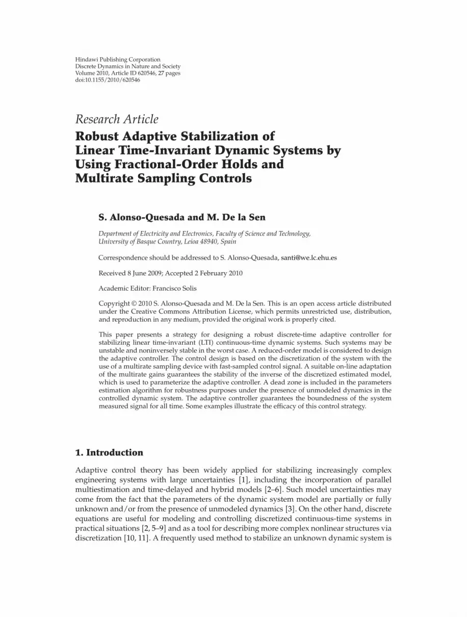
Figure 1: Continuous-time dynamic system and reference model measured signals.

302520151050

t

u(t)

−120

−100

−80

−60

−40

−20

0

20

40

60

80

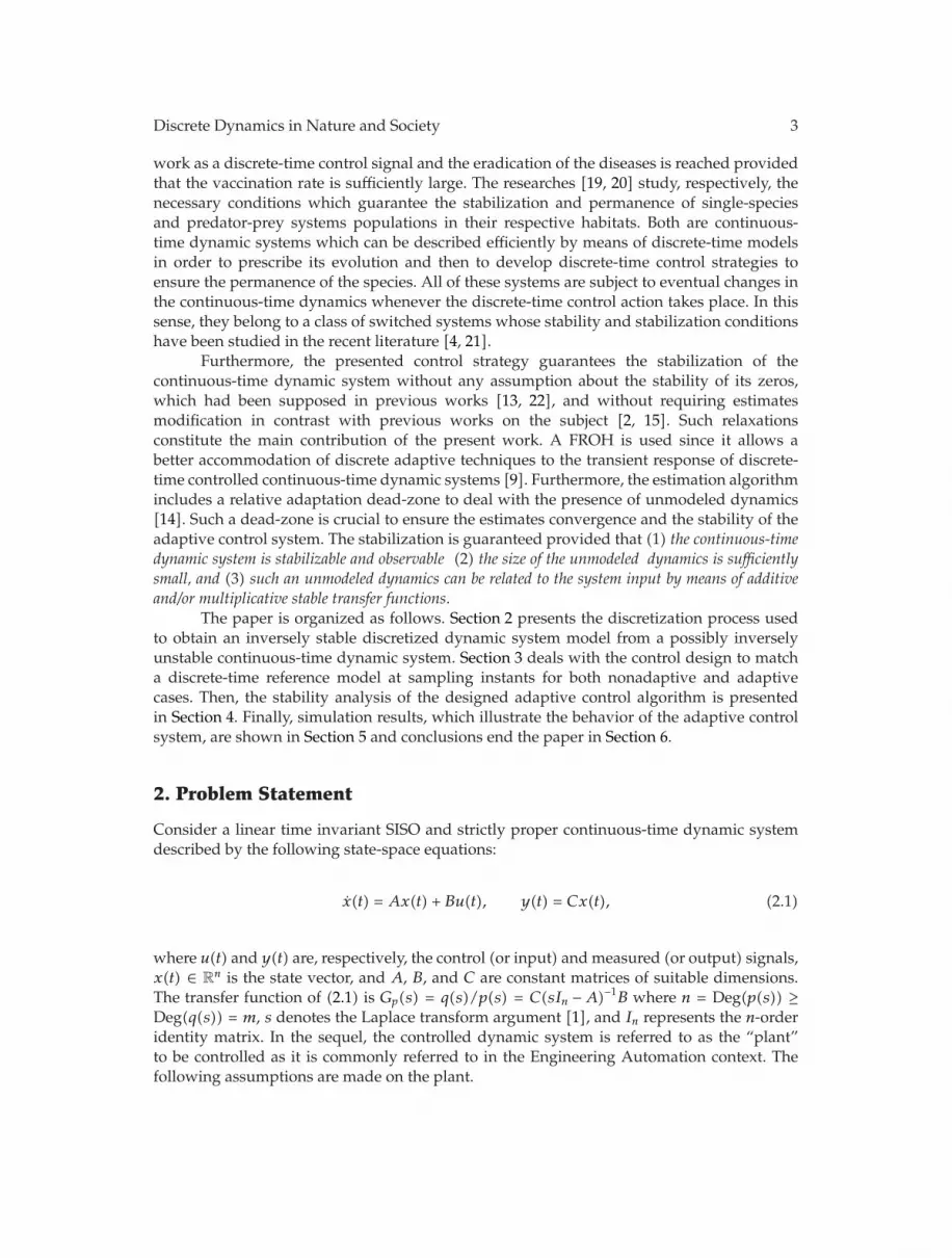
Figure 2: Continuous-time dynamic system control signal.

invariant although the estimates θb,i(k), for i ∈ {1, . . . ,N}, are time varying. Furthermore,the controller parameterization can be obtained from R(z) = B′(z) and equations similar to(3.3) by replacing the discretized plant polynomial A(z) by its corresponding estimated oneat the current sampling instant, namely, A(z, k) [2]. In this context, the polynomials T(z) andR(z) have to be calculated once for all since Bm(z), As(z) and B′(z), are time invariant. Onthe contrary, S(z), now being S(z, k), is updated at each running sampling instant since thepolynomial A(z, k) is time varying.


302520151050

t

a1

a2

−14

−12

−10

−8

−6

−4

−2

0

2

4

6

Figure 3: Estimates of the parameters a1 and a2.

302520151050

t

b1,1

b1,2

b1,3

0

0.1

0.2

0.3

0.4

0.5

0.6

0.7

0.8

0.9

Figure 4: Estimates of the parameters b1,1, b1,2 and b1,3.


302520151050

t

b2,1

b2,2

b2,3

−1.2

−1.1

−1

−0.9

−0.8

−0.7

−0.6

−0.5

−0.4

−0.3

−0.2


302520151050

t

b3,1

b3,2

b3,3

−0.1

0

0.1

0.2

0.3

0.4

0.5

0.6

0.7

0.8



302520151050

t

α1

α2

α3

−6

−4

−2

0

2

4

6

Figure 7: Multirate gains evolution.

20181614121086420

t

y(t)

−300

−200

−100

0

100

200

300

400

(a)

3029282726252423222120

t

y(t)

−2.5

−2

−1.5

−1

−0.5

0

0.5

1

1.5

2

2.5×1010

(b)

Figure 8: Continuous-time dynamic system measured signal without dead-zone in the parametersestimation algorithm.


The time-varying multirate gains αj(k) are used to calculate the plant input within theinter sample period via (2.4). Then, a time-varying input-output relation for the discretizedplant is derived by following similar steps to those in Section 2.1. In this sense, one obtains

y(k − �)

= C0

{Fn0−�x0(k − n0) + H1(k − � − 1)u(k − � − 1) +

n0−1∑i=�+1

Fi−�−1(FH1(k − i − 1) + H2(k − i)

)

×u(k − i − 1) + Fn0−�−1H2(k − n0)u(k − n0 − 1)

}+ η(k − �)

(3.5)

for � ∈ {0, 1, . . . , n0 − 1}, where H1(i) and H2(i) are obtained from equations similar to thosein (2.6) by replacing αj by αj(i), for i ∈ {k − 1, . . . , k − n0} and j ∈ {1, . . . ,N}. Then

Yv(k − 1) = Vx0(k − n0) + Πv(k − 1) + Φ(k − 2, . . . , k − n0)Uv(k − 2), (3.6)

where Yv(k − 1), V , Πv(k − 1), and Uv(k − 2) are defined in (2.11) while

Φ(k − 2, . . . , k − n0) =

⎡⎢⎢⎢⎢⎢⎢⎢⎢⎢⎢⎢⎢⎢⎣

0 0 · · · 0 0

Φ2,1 Φ2,2 · · · 0 0

Φ3,1 Φ3,2 · · · 0 0

......

. . ....

...

Φn0−1,1 Φn0−1,2 · · · Φn0−1,n0−1 0

Φn0,1 Φn0,2 · · · Φn0,n0−1 Φn0,n0

⎤⎥⎥⎥⎥⎥⎥⎥⎥⎥⎥⎥⎥⎥⎦

(3.7)

with Φi,j = C0Fi−j−1(FH1(k − n0 + j − 2) + H2(k − n0 + j − 1)), Φi,i = C0H1(k − n0 + i − 2), and

Φi,1 = C0Fi−2H2(k−n0) for i, j ∈ {2, 3, . . . , n0} and i > j. By substituting in (3.5) the expression

for x0(k − n0), obtained from (3.6), for � = 0 it follows that

y(k) = −n0∑i=1

aiy(k − i) + C0H1(k − 1)u(k − 1)

+n0−1∑i=1

{C0F

i−1(FH1(k − i − 1) + H2(k − i)

)−

[C0F

n0V −1Φ(k − 2, . . . , k − n0)]n0−i+1

}

× u(k − i − 1) +(C0F

n0−1H2(k − n0) −[C0F

n0V −1Φ(k − 2, . . . , k − n0)]

1

)u(k − n0 − 1)

+n0∑i=1

aiη(k − i) + η(k),

(3.8)


or

y(k) = −n0∑i=1

aiy(k − i) + C0H1(k − 1)u(k − 1)

+n0−1∑i=1

{C0F

i−1(FH1(k − 1) + H2(k − 1)

)−

[C0F

n0V −1Φ(k − 1)]n0−i+1

}u(k − i − 1)

+(C0F

n0−1H2(k − 1) −[C0F

n0V −1Φ(k − 1)]

1

)u(k − n0 − 1) +

n0∑i=1

aiη(k − i)

+ η(k) + Λα(k − 1),(3.9)

where

Λα(k − 1)

=n0−1∑i=1

{C0F

i−1(FΔH1(k − i − 1) + ΔH2(k − i)

)−

[C0F

n0V −1ΔΦ]n0−i+1

}u(k − i − 1)

+(C0F

n0−1ΔH2(k − n0) −[C0F

n0V −1ΔΦ]

1

)u(k − n0 − 1)

(3.10)

with ΔH�(k−i−1) = H�(k−i−1)−H�(k−1), for � = 1, 2, and ΔΦ = Φ(k−2, . . . , k−n0)−Φ(k−1).Note that Ω(k) =

∑n0i=1 aiη(k−i)+η(k) arises from the unmodeled dynamics of the continuous-

time plant while Λα(k − 1) comes from the fact that the multirate gains are time varying. Bothterms constitute the unmodeled dynamics for the discretized plant model. On one hand, thelatter tends to zero if the multirate gains converge to constant values. On the other hand, theformer is such that

|Ω(k)| ≤ Ω(k) = μ1ρ(k) + μ2 (3.11)

for some known real constants μ1 ≥ 0 and μ2 ≥ 0, where

ρ(k) = Sup0≤k′≤k

{∣∣∣wTx(k′

)∣∣∣σk−k′} (3.12)

for all k ∈ Z+0 , some known constant vector w, and some known real constant σ ∈ (0, 1) with

x(k) =[y(k − 1) · · · y(k − n0) u(k − 1) · · · u(k −N)

]T (3.13)


in view of Assumption 1(ii) [14]. Finally, one can express the discretized plant model as

y(k) = −n0∑i=1


bi(k − 1)u(k − i) + Ω(k) + Λα(k − 1)

= −n0∑i=1


N∑j=1

bi,j αj(k − 1)u(k − i) + Ω(k) + Λα(k − 1)

= θT ϕ(k − 1) + Ω(k) + Λα(k − 1),

(3.14)

where ϕ(k − 1) is built like ϕ(k − 1) in (2.17) by replacing the components of u(k − i), namely,αju(k − i), by the corresponding αj(k − 1)u(k − i), for i, j ∈ {1, . . . ,N}.

The algorithm used to obtain an on-line adaptation θ(k) of the unknown parametersvector θ is described below.

3.2.1. Estimation Algorithm

An “a priori” estimated parameters vector is obtained by using a recursive least-squaresalgorithm defined by

θ0(k) = θ0(k − 1) +s(k)P(k − 1)ϕn(k − 1)e0

n(k)

γ(k) + s(k)ϕTn(k − 1)P(k − 1)ϕn(k − 1),

P(k) = P(k − 1) −s(k)P(k − 1)ϕn(k − 1)ϕTn(k − 1)P(k − 1)

γ(k) + s(k)ϕTn(k − 1)P(k − 1)ϕn(k − 1)

(3.15)

for all k ∈ Z+, where ϕn(k − 1) = ϕ(k − 1)/(1 + ‖ϕ(k − 1)‖), P(k − 1) is initialized such that

P(0) = PT (0) > 0 (denoting positive definiteness), γ(k) > 0, e0n(k) = e0(k)/(1 + ‖ϕ(k − 1)‖)

with

e0(k) = −θ0T (k − 1)ϕ(k − 1) + Ω(k) + Λα(k − 1) (3.16)

being the “a priori” estimation error as well as θ0(k − 1) = θ0(k − 1) − θ the “a priori”parametrical error, and s(k) is a relative adaptation dead-zone defined as

s(k) =

⎧⎪⎪⎨⎪⎪⎩

0 if e0an(k) ≤ μηan(k),

f(k)

e0an(k)

otherwise(3.17)

for some μ > 1, where e0an(k) = ((e0

n(k))2 + ϕTn(k − 1)P 2(k − 1)ϕn(k − 1))

1/2is an augmented

normalized error, ηan(k) = (1 + γ−1(k)ϕTn(k − 1)P(k − 1)ϕn(k − 1))1/2ηTn(k) with ηTn(k) =


ηT (k)/(1 + ‖ϕ(k − 1)‖) and ηT (k) being an upper bound for |ηT (k)| = |Ω(k) + Λα(k − 1)|,and

f(k) =

⎧⎨⎩

0 if e0an(k) ≤ μηan(k),

e0an(k) − μηan(k) otherwise.

(3.18)

This algorithm provides an estimation θ0(k) of the parameters vector. Then, an “a posteriori”estimates vector is obtained as follows.

Estimates Modification

This algorithm consists of three main steps as follows.

Step 1. Build the matrix M0(k) = [b0i,j(k)] ∈ R

N×N , for i, j ∈ {1, 2, . . . ,N}, from the “a priori”

estimates θ0b,i(k), included in θ0(k), of the corresponding θb,i defined in (2.17).

Step 2. M(k) = M0(k) :

If |Det(M(k))| ≥ δ0 then θb,i(k) = θ0b,i(k)

else while |Det(M(k))| < δ0

M(k) = M(k) + δIN

end;

for i = 1 to N

θb,i(k) = Mi(k)

end,

end.

Step 3. θ(k) = [θ0Ta (k) θTb,1(k) θTb,2(k) · · · θTb,N(k)]

T,

for some positive real constants δ 1 and δ0 1, and where Mi(k) denotes the i-th row ofM(k) and IN the identity matrix of dimension N ×N.

Once the estimated parameters are updated, the multirate gains vector g(k) =[α1(k) · · · αN(k)]T is calculated from an equation similar to (2.15) by replacing the matrixM by M(k) = [bi,j(k)] ∈ R

N×N .

Remark 3.1. (i) The proposed estimates modification process avoids that the time-varyingmatrix M(k) be close to a singular one. In this way, a bounded vector of multirate gains isobtained at all sampling instants.

(ii) Note that the estimate θ0a(k) corresponding to the parameters of θa is not affected

by the modification algorithm. In fact, such a modification only affects the entries in the maindiagonal of M0(k). Also, note that the instruction while of the second step is executed afinite number of times since there exists a finite integer number � such that |Det[M(k)]| =|Det[M0(k)+�δIN]| = |(�δ)N +f0(δ, θ0

b,i(k))| ≥ δ0 for i ∈ {1, . . . ,N} and some function f0(·, ·).


(iii) From (3.10) to (3.13) and the construction of ϕ(k − 1), there exist some realconstants υi ≥ 0, for i ∈ {1, 2, 3, 4} such that the sequences {η1(k)}, with η1(k) = υ1‖ϕ(k −1)‖ + υ2, and {η2(k)}, with η2(k) = υ3‖x(k − 1)‖ + υ4, are both upper bounds for {|ηT (k)|}.

The estimation algorithm together with such a multirate gains adaptation possessesthe following properties.

Lemma 3.2 (main properties of the estimation algorithm). (i) P(k) is uniformly bounded for allk ∈ Z

+0 , and it asymptotically converges to a finite, at least semidefinite positive, limit as k → ∞.(ii) θ0(k) and θ(k) are uniformly bounded for all samples and converge to finite limits.(iii) f(k) <∞ for all k ∈ Z

+0 and limk→∞f(k) = 0.

(iv) The vector g(k) is bounded for all samples and converges to a finite limit.

The proof is made in Appendix A.

4. Stability Analysis

The plant discretized model can be written as follows:

y(k) = y(k) + e(k) = θT (k − 1)ϕ(k − 1) + e(k)

= −n0∑i=1

ai(k − 1)y(k − i) +N∑i=1

N∑j=1

bi,j(k − 1)αj(k − 1)u(k − i) + e(k)

= −n0∑i=1

ai(k − 1)y(k − i) +N∑i=1

b′iu(k − i) + e(k)

(4.1)

and the adaptive control law (3.1), replacing S(z) by S(k, z), as

u(k) =1b′1

{N−1∑i=1

(s1(k − 1)ai(k − 1) − si+1(k − 1))y(k − i)

+ σ(β)s1(k − 1)aN(k − 1)y(k −N) −

N−1∑i=1

(s1(k − 1)b′i + b

′i+1

)u(k − i)

−s1(k − 1)b′Nu(k −N) +N∑i=1

tic(k − i + 1) − s1(k − 1)e(k)

},

(4.2)

where S(z, k − 1) =∑N

i=1 si(k − 1)zN−i, T(z) =∑N

i=1 tizN−i, R(z) = B′(z) =

∑Ni=1 b

′izN−i, and the

binary-valued function

σ(β)=

⎧⎨⎩

1 if β = 0,

0 otherwise(4.3)


have been used. By combining (4.1) and (4.2), the discrete-time closed-loop system can bewritten as

x(k) = Λ(k − 1)x(k − 1) + Ψ1(k − 1)e(k) +1b′1

Ψ2

N∑i=1

tic(k − i + 1), (4.4)

where

x(k) =[y(k) y(k − 1) · · · y(k − n0 + 1) u(k) u(k − 1) · · · u(k −N + 1)

]T,

Ψ1(k − 1) =

⎡⎢⎢⎣1 0 · · · 0 −s1(k − 1)/b′1︸︷︷︸

n0+1

0 · · · 0

⎤⎥⎥⎦T

∈ R(n0+N)×1,

Ψ2 =

⎡⎢⎣0 0 · · · 0 1︸︷︷︸

n0+1

0 · · · 0

⎤⎥⎦T

∈ R(n0+N)×1,

Λ(k − 1)

=

⎡⎢⎢⎢⎢⎢⎢⎢⎢⎢⎢⎢⎢⎢⎢⎢⎢⎢⎢⎢⎢⎢⎢⎢⎢⎢⎢⎣

−a1(k − 1) −a2(k − 1) · · · −an0−1(k − 1) −an0 (k − 1) b′1 b′2 · · · b′N−1 b′N

1 0 · · · 0 0 0 0 · · · 0 0

0 1 · · · 0 0 0 0 . . . 0 0

......

. . ....

......

.... . .

......

0 0 · · · 1 0 0 0 · · · 0 0

f1(k − 1) f2(k − 1) · · · fn0−1(k − 1) fn0 (k − 1) −h1(k − 1) −h2(k − 1) · · · −hN−1(k − 1) −hN(k − 1)

0 0 · · · 0 0 1 0 · · · 0 0

0 0 · · · 0 0 0 1 · · · 0 0

......

. . ....

......

.... . .

......

0 0 · · · 0 0 0 0 · · · 1 0

⎤⎥⎥⎥⎥⎥⎥⎥⎥⎥⎥⎥⎥⎥⎥⎥⎥⎥⎥⎥⎥⎥⎥⎥⎥⎥⎥⎦

(4.5)

with fn0(k − 1) = (1/b′1)[s1(k − 1)an0(k − 1) − (1 − σ(β))sn0+1(k − 1)], fi(k − 1) = (1/b′1)[s1(k −1)ai(k − 1)− si+1(k − 1)], for i ∈ {1, 2, . . . , n0 − 1}, hN(k − 1) = (b′N/b

′1)s1(k − 1), and hi(k − 1) =

(1/b′1)[s1(k − 1)b′i + b′i+1] for i ∈ {1, 2 , . . . ,N − 1}. Note that ai(k − 1) are uniformly bounded

from Lemma 3.2. Also, si(k − 1) are uniformly bounded from the resolution of an equationsimilar to (3.3) by replacing the polynomials A(z) and S(z) by A(k − 1, z) and S(k − 1, z),respectively. The following theorem, whose proof is made in Appendix B, establishes the mainstability result of the adaptive control system.

Theorem 4.1 (main stability result). (i) The adaptive control law stabilizes the plant model (3.14)in the sense that {u(k)} and {y(k)} are bounded for all finite initial states and any bounded referenceinput sequence {c(k)} subject to Assumption 1.

(ii) The control and measured signals of the continuous-time dynamic system, u(t) and y(t),are bounded for all t.


5. Simulations

A continuous-time dynamic system defined by the matrices

A =

⎡⎢⎢⎢⎢⎢⎣

0 17.5 0 0

1 1.5 0 0

0 0 −10 0

0 1 0 −15

⎤⎥⎥⎥⎥⎥⎦, B =

⎡⎢⎢⎢⎢⎢⎣

−1

1

0.05

0

⎤⎥⎥⎥⎥⎥⎦, C =

[0 1 1 0.05

](5.1)

in the state-space and by the transfer function

G(s) =s − 1

(s − 5)(s + 3.5)

(1 +

0.05s + 15

)+

0.05s + 10

(5.2)

is considered. This plant is supposed unknown and the adaptive control strategy describedin the paper will be used to stabilize it. Such a strategy is based on a discretization processusing a FROH with β = 0.3 for a slow sampling time T = 0.3 and a multirate device withN = 3 to place the zeros of the estimated discretized plant model within the stability domain.The time-varying discrete transfer-like function corresponding to such an estimated modelis Gd(z, k) = (Bd(z, k)/Ad(z, k)) = ((b1(k)z2 + b2(k)z + b3(k))/z(z2 + a1(k)z + a2(k))) withbi(k) =

∑3j=1 bij(k)αj(k), for all i ∈ {1, 2, 3} and all k ∈ Z

+0 . The estimates bij(k) are provided

by the estimation algorithm described in Section 3.2.1 with γ(k) = 0.01 for all k ∈ Z+0 and

initialized with P(0) = 55 × I11, θa(0) = [−12.079 3.92]T , θb,1(0) = [0.492 0.379 0.33]T ,θb,2(0) = [−0.435 − 0.556 − 0.759]T , and θb,3(0) = [0.019 0.066 0.139]T . Also, ηT (k) =υ1‖ϕ(k − 1)‖ + υ2, with υ1 = 0.0055 and υ2 = 0.01, is used as upper bound for |ηT (k)| andμ = 1.1 for the dead-zone included in such an algorithm. The values δ = δ0 = 10−6 aretaken in Step 2 of the estimates modification procedure. The gains αj(k), for j ∈ {1, 2, 3},are on-line updated in order to fix B(z, k) to the polynomial B′(z) = z2 − 0.25. The controlobjective is to match the reference model given by Gm(z) = ((z2 + 0.1z + 0.083)/(z3 +0.3z2 − 0.09z − 0.027)). Figures 1 and 2 display, respectively, the continuous-time dynamicsystem measured and control signals under a unitary step external input sequence {c(k)}.Note that both signals are bounded for all time; that is, the stabilization of the closed-loopsystem is reached. Furthermore, the plant output sequence {y(k)} converges asymptoticallyto {ym(k)}. Figures 3, 4, 5, and 6 show the evolution of the estimates, included as components

of θ(k) = [θTa (k) θTb,1(k) θT

b,2(k) θTb,3(k)]

T, during the simulation while Figure 7 displays

the evolution of the multirate gains g(k) = [α1(k) α2(k) α3(k)]T . Note that therefore the

estimated parameters as the multirate gains converge to a set of constant values as t tendsto infinite. Finally, Figures 8(a) and 8(b) show the evolution of the continuous-time dynamicsystem measured signal, each one in a different time interval, if the same estimation algorithmwithout the dead-zone is used to stabilize the system. The behavior of the adaptive controlsystem is improved with the inclusion of the relative adaptation dead-zone in this particularexample as one can see by comparing the signal y(t) in Figure 1 with those displayed inFigures 8(a) and 8(b). This conclusion cannot be generalized for all cases since one can searchexamples where the inclusion of the dead-zone does not improve the performance of thecontrol system. However, the inclusion of the relative dead-zone guarantees the stabilization


of the adaptive control system under the presence of unmodeled dynamics, which is whatjustifies its inclusion in the parameters estimation algorithm.

6. Conclusions

An adaptive control strategy for stabilizing linear time-invariant continuous-time dynamicsystems, being possibly of inverse nonstable, and subject to the presence of unmodeleddynamics has been presented. The control design is based on the discrete-time modelreference adaptive (MRAC) control method. Therefore, an inversely stable discretized modelof the continuous-time dynamic system is required to achieve the stabilization objective whilematching a freely chosen discrete-time reference model. Such a requirement is guaranteedby using a fractional-order hold (FROH) combined with a multirate device with fastsampling input in the discretization process of the continuous-time system. In this context, anestimation algorithm is used to on-line update the multirate gains such that the zeros of thetransfer-like function associated to the estimated model of the discretized system are withinthe open-unit complex circle at all sampling instants. The parameters of such an estimatedmodel are used to on-line parameterize the adaptive control law. The estimation algorithmincludes a relative adaptation dead-zone for dealing with the presence of unmodeleddynamics. The stability of the adaptive control system is proved under the assumption thatthe nominal model of the continuous-time dynamic system is observable, an upper-bound ofits order is known, and the contribution of the unmodeled dynamics to the system output issufficiently small. Finally, the performance of the adaptive control system is shown by meansof simulation results. The stabilization of the system is manifested although the intersamplebehavior of the measured signal could be improved. A future potential research may be theuse of the same control technique in a multiestimation scheme for improving such an inter-sample behavior.

Appendices

A. Proof of Lemma 3.2

(i) Equation (32b) and the matrix inversion lemma lead to P−1(k) = P−1(k − 1) +γ−1(k)s(k)ϕn(k − 1)ϕTn(k − 1) > 0 for all k ∈ Z

+ provided that P(0) = PT (0) > 0. Then, {P(k)}is a nonnegative and monotonic nonincreasing matrix sequence. Thus, 0 ≤ P(k) ≤ P(0) andP(k) asymptotically converges to a finite limit as k → ∞.

(ii) By considering the nonnegative sequence V (k) = θ0T (k)P−1(k)θ0(k) + Tr{P(k)}and using the matrix inversion lemma in (32b), it follows that

V (k) − V (k − 1) = −s(k)

((e0an(k)

)2 −(ηan(k)

)2)

γ(k) + s(k)ϕTn(k − 1)P(k − 1)ϕn(k − 1)

≤ −((μ2 − 1

)/μ2)s(k)(e0

an(k))2

γ(k) + s(k)ϕTn(k − 1)P(k − 1)ϕn(k − 1)

≤ −((μ2 − 1

)/μ2)(f(k))2

γ(k) + s(k)ϕTn(k − 1)P(k − 1)ϕn(k − 1)≤ 0,

(A.1)


where (32a) and the definition of the “a priori” estimation error have been used. Then, V (k) ≤V (0) < ∞ and ‖θ0(k)‖ ≤ (λmax{P(0)}/λmin{P(0)})‖θ0(0)‖ + λmax{P(0)}Tr{P(0)} < ∞ whereλmax(M) and λmin(M) denote the maximum and the minimum eigenvalues of the matrix M,respectively. It implies that θ0(k) and then also θ0(k) are uniformly bounded. Then, θ(k) isalso bounded since the modification algorithm guarantees the boundedness of M(k) providedthat θ0(k) is bounded. Moreover, V (k) asymptotically converges to a finite limit as k → ∞from its definition and the fact that such a sequence is nonnegative and monotonic non-increasing. Then, θ0(k), and also θ0(k), converges to a finite limit as k → ∞ since P(k) alsoconverges as it has been proved in (i). Then, M(k) and θ(k) also converge to finite limits ask → ∞.

(iii) From (A.1), it follows that

μ2 − 1μ2

k∑i=1

(f(i)

)2

γ(i) + s(i)ϕTn(i − 1)P(i − 1)ϕn(i − 1)≤ V (0) − V (k) ≤ V (0) <∞ (A.2)

for all k ∈ Z+. Then f(k) <∞ for all k ∈ Z

+ and also limk→∞f(k) = 0.(iv) The boundedness and convergence of the estimation model parameters vector

together with the nonsingularity of matrix M(k) (guaranteed by the modification algorithm)imply the boundedness and convergence of the vector g(k) obtained by resolution of (2.15)replacing M by M(k).

B. Proof of Theorem 4.1

(i) Λ(k − 1) is bounded since the estimated plant parameters ai(k − 1), for i ∈ {1, . . . , n0}, andthe controller parameters sj(k − 1), for j ∈ {1, . . . ,N}, are bounded thanks to θ(k − 1) andg(k − 1) are bounded for all k ∈ Z

+, see Lemma 3.2. The eigenvalues of Λ(k − 1) are in |z| < 1since they are the roots of Am(z), As(z) and B′(z), which are stable. Furthermore,

k∑k′=k0+1

∥∥Λ(k′

)−Λ

(k′ − 1

)∥∥2 ≤ γ0 + γ1(k − k0) (B.1)

for all integers k > k0 ≥ 0 and some positive real constants γ0 and γ1, with γ1 being sufficientlysmall by using slow enough estimation rates via a suitable P(0) in (32b). Thus, the unforcedtime-varying system x(k) = Λ(k − 1)x(k − 1) is exponentially stable and its transition matrixφ(k, k′) =

∏k−1j=k′Λ(j) satisfies ‖φ(k, k′)‖ ≤ ρ1σ

k−k′0 for all integer k ≥ k′ where σ0 ∈ (0, 1) is

an upper bound for the absolute value of the closed-loop stability abscissa and ρ1 is a non-dependent constant [2]. Note that σ0 depends on the freely chosen reference model. From(4.4),

x(k) = φ(k, k0)x(k0) +k∑

k′=k0

φ(k, k′

)(Ψ1

(k′ − 1

)e(k′

)+

1b′1

Ψ2

N∑i=1

tic(k′ − i + 1

)). (B.2)


Then,

‖x(k)‖ ≤ ρ1σk−k00 ‖x(k0)‖ +

k∑k′=k0

ρ1σk−k′0

(ρ2 + ρ3

∣∣e(k′)∣∣), (B.3)

for some positive real constants ρi, i ∈ {1, 2, 3}, since Ψ1(k) is uniformly bounded andprovided that the sequence {c(k)} is bounded. From (3.16) and (4.1), it follows that e(k) =

e0(k) + (θ0(k − 1) − θ(k − 1))Tϕ(k − 1), and then

|e(k)| ≤∣∣∣e0(k)

∣∣∣ + �(k)δ∥∥ϕ(k − 1)∥∥ (B.4)

where �(k) denotes the finite number of times that the instruction while in the Step 2 of theestimates modification algorithm is executed at the current sampling time kT . By substituting(B.4) in (B.3), one obtains

‖x(k)‖ ≤ ρ4 +k∑

k′=k0

ρ5σk−k′0

(∣∣∣e0(k′)∣∣∣ + �(k′)δ∥∥ϕ(k′ − 1)∥∥)

, (B.5)

for some positive real constants ρ4 and ρ5 from the boundedness of x(k0). By using that ϕn(k−1) = ϕ(k − 1)/(1 + ‖ϕ(k − 1)‖) and e0

n(k) = e0(k)/(1 + ‖ϕ(k − 1)‖), it follows that

‖x(k)‖ ≤ ρ4 +k∑

k′=k0

ρ5σk−k′0

(∣∣∣e0n

(k′

)∣∣∣ + �(k′)δ∥∥ϕn(k′ − 1)∥∥)(

1 +∥∥ϕ(k′ − 1

)∥∥)

≤ ρ4 +k∑

k′=k0

ρ6σk−k′0 e0

an

(k′

)(1 +

∥∥ϕ(k′ − 1)∥∥) (B.6)

for some positive real constant ρ6 and, also, by taking into account that (|e0n(k)|+�(k)δ‖ϕn(k−

1)‖) ≤ ρ′((e0n(k))

2 + ϕTn(k − 1)P 2(k − 1)ϕn(k − 1))1/2

= ρ′e0an(k) for some positive real constant

ρ′. Moreover, from (B.6),

‖x(k)‖ ≤ ρ4 +k∑

k′=k0

ρ6σk−k′0 μ

(1 +

ϕTn(k′ − 1)P(k′ − 1)ϕn(k′ − 1)

γ(k′)

)1/2

ηT(k′

)

+k∑

k′=k0

ρ6σk−k′0 f

(k′

)(1 +

∥∥ϕ(k′ − 1)∥∥) (B.7)


where e0an(k

′) has been split into the two additive terms f(k′) and e0an(k

′) − f(k′) ≤ μηan(k′).Then,

‖x(k)‖ ≤ ρ7 +ρ6μυ3

1 − σ0Supk0≤k′≤k

⎧⎨⎩

(1 +

ϕTn(k′ − 1)P(k′ − 1)ϕn(k′ − 1)

γ(k′)

)1/2⎫⎬⎭ Sup

k0≤k′≤k

{∥∥x(k′)∥∥}

+k∑

k′=k0

ρ6σk−k′0 f

(k′

)(1 +

∥∥ϕ(k′ − 1)∥∥) (B.8)

for some positive constant ρ7 by taking into account that ηT (k) = υ3‖x(k − 1)‖ + υ4 (seeRemark 3.1(iii)). Furthermore, the right-hand side of (B.8) is monotonic nondecreasing in k.Then, for k � k0, it follows that

‖x(k)‖ ≤ ρ8 +k∑

k′=k0

ρ9σk−k′0 f

(k′

)(1 +

∥∥ϕ(k′ − 1)∥∥)

(B.9)

provided that υ3 < ((1 − σ0)/ρ6μ)(Supk0≤k′≤k{(1 + ϕTn(k′ − 1)P(k′ − 1)ϕn(k′ − 1)/γ(k′))1/2})

−1,

for some positive constants ρ8 and ρ9. By taking into account that ‖g(k)‖ is bounded for allk ∈ Z

+0 , then

∥∥ϕ(k − 1)∥∥ ≤ ρ10 + ρ11 Sup

k0≤k′≤k

{∥∥x(k′ − 1)∥∥}

(B.10)

for some positive constants ρ10 and ρ11. By substituting (B.10) in (B.9) and by taking intoaccount that the right-hand side of (B.9) is monotonic nondecreasing in k, it follows that,

Supk0≤k′≤k

{∥∥x(k′)∥∥}≤ ρ12 +

k∑k′=k0

ρ13f(k′

)Sup

k0≤k′′≤k′

{∥∥x(k′′ − 1)∥∥}

(B.11)

for some positive constants ρ12 and ρ13, where the boundedness of f(k) has been used, seeLemma 3.2. The use of Gronwall’s Lemma [24] in (B.11) leads to

Supk0≤k′≤k

{∥∥x(k′)∥∥2}≤ ρ14 +

k∑i=k0

⎛⎝∏

i<j<k

(1 + ρ15f

2(j))⎞⎠ρ14ρ15f

2(i) <∞ (B.12)

for some positive constants ρ14 and ρ15. It implies that the sequence ‖x(k)‖ is bounded for allk ∈ Z

+ provided that the initial condition is bounded. Then, the sequences {u(k)} and {y(k)}are also bounded.

(ii) The adaptive control algorithm ensures that there are not finite escape times, andthen the boundedness of the sequences {u(k)} and {y(k)} guarantees that of the continuous-time signals from continuity arguments of the solutions of differential equations.


Acknowledgments

The authors are very grateful to MCYT for its support through Grants nos. DPI2006-00714and DPI 2009-07197. They are also very grateful to the reviewers for their useful comments,which have helped to improve the previous versions of the manuscript.

References

[1] P. A. Ioannou and J. Sun, Robust Adaptive Control, Prentice-Hall, Englewood Cliffs, NJ, USA, 1996.[2] S. Alonso-Quesada and M. De la Sen, “Robust adaptive control of discrete nominally stabilizable

plants,” Applied Mathematics and Computation, vol. 150, no. 2, pp. 555–583, 2004.[3] S. Alonso-Quesada and M. De la Sen, “Robust adaptive stabilizer for linear systems with imperfectly

known point delays using a multi-estimation model,” Dynamics of Continuous, Discrete & ImpulsiveSystems. Series B, vol. 15, no. 5, pp. 683–708, 2008.

[4] M. De la Sen and A. Ibeas, “On the global asymptotic stability of switched linear time-varying systemswith constant point delays,” Discrete Dynamics in Nature and Society, vol. 2008, Article ID 231710, 31pages, 2008.

[5] M. De la Sen and A. Ibeas, “Stability results of a class of hybrid systems under switched continuous-time and discrete-time control,” Discrete Dynamics in Nature and Society, vol. 2009, Article ID 315713,28 pages, 2009.

[6] A. Ibeas, M. De la Sen, and S. Alonso-Quesada, “Stable multi-estimation model for single-inputsingle-output discrete adaptive control systems,” International Journal of Systems Science, vol. 35, no. 8,pp. 479–501, 2004.

[7] M. De la Sen and S. Alonso-Quesada, “Model matching via multirate sampling with fast sampledinput guaranteeing the stability of the plant zeros: extensions to adaptive control,” IET Control Theory& Applications, vol. 1, no. 1, pp. 210–225, 2007.

[8] S. Liang and M. Ishitobi, “Properties of zeros of discretised system using multirate input and hold,”IEE Proceedings: Control Theory and Applications, vol. 151, no. 2, pp. 180–184, 2004.

[9] S. Liang, M. Ishitobi, and Q. Zhu, “Improvement of stability of zeros in discrete-time multivariablesystems using fractional-order hold,” International Journal of Control, vol. 76, no. 17, pp. 1699–1711,2003.

[10] B. Iricanin and S. Stevic, “On some rational difference equations,” Ars Combinatoria, vol. 92, pp. 67–72,2009.

[11] S. Stevic, “On a generalized max-type difference equation from automatic control theory,” NonlinearAnalysis: Theory, Methods & Applications, vol. 72, no. 3-4, pp. 1841–1849, 2010.

[12] K. S. Narendra and A. M. Annaswamy, Stable Adaptive Systems, Prentice-Hall, Englewood Cliffs, NJ,USA, 1989.

[13] P. A. Ioannou and Datta, “Robust adaptive control: a unified approach,” Proceedings of the IEEE, vol.79, no. 12, pp. 1736–1768, 1991.

[14] R. H. Middleton, G. C. Goodwin, D. J. Hill, and D. Q. Mayne, “Design issues in adaptive control,”IEEE Transactions on Automatic Control, vol. 33, no. 1, pp. 50–58, 1988.

[15] S. Alonso-Quesada and M. De la Sen, “Robust adaptive control with multiple estimation models forstabilization of a class of non-inversely stable time-varying plants,” Asian Journal of Control, vol. 6, no.1, pp. 59–73, 2004.

[16] K. G. Arvanitis, “An algorithm for adaptive pole placement control of linear systems based ongeneralized sampled-data hold functions,” Journal of the Franklin Institute, vol. 336, no. 3, pp. 503–521, 1999.

[17] M. J. Błachuta, “On approximate pulse transfer functions,” IEEE Transactions on Automatic Control, vol.44, no. 11, pp. 2062–2067, 1999.

[18] L. Chen and L. Chen, “Permanence of a discrete periodic Volterra model with mutual interference,”Discrete Dynamics in Nature and Society, vol. 20089, Article ID 205481, 9 pages, 2009.

[19] Y.-H. Fan and L.-L. Wang, “Permanence for a discrete model with feedback control and delay,”Discrete Dynamics in Nature and Society, vol. 2008, Article ID 945109, 8 pages, 2008.

[20] C. Wei and L. Chen, “A delayed epidemic model with pulse vaccination,” Discrete Dynamics in Natureand Society, vol. 2008, Article ID 746951, 12 pages, 2008.

[21] H. R. Karimi, M. Zapateiro, and N. Luo, “New delay-dependent stability criteria for uncertain neutral


systems with mixed time-varying delays and nonlinear perturbations,” Mathematical Problems inEngineering, vol. 2009, Article ID 759248, 22 pages, 2009.

[22] G. Tao and P. A. Ioannou, “Model reference adaptive control for plants with unknown relativedegree,” IEEE Transactions on Automatic Control, vol. 38, no. 6, pp. 976–982, 1993.

[23] G. C. Goodwin and K. S. Sin, Adaptive Filtering Prediction and Control, Prentice-Hall, Englewood Cliffs,NJ, USA, 1984.

[24] C. A. Desoer and M. Vidyasagar, Feedback Systems: Input-Output Properties, Academic Press, New York,NY, USA, 1975.

Submit your manuscripts athttp://www.hindawi.com

Hindawi Publishing Corporationhttp://www.hindawi.com Volume 2014

MathematicsJournal of


Mathematical Problems in Engineering

Hindawi Publishing Corporationhttp://www.hindawi.com

Differential EquationsInternational Journal of

Volume 2014

Applied MathematicsJournal of


Probability and StatisticsHindawi Publishing Corporationhttp://www.hindawi.com Volume 2014

Journal of


Mathematical PhysicsAdvances in

Complex AnalysisJournal of


OptimizationJournal of


CombinatoricsHindawi Publishing Corporationhttp://www.hindawi.com Volume 2014

International Journal of


Operations ResearchAdvances in

Journal of


Function Spaces

Abstract and Applied AnalysisHindawi Publishing Corporationhttp://www.hindawi.com Volume 2014

International Journal of Mathematics and Mathematical Sciences


The Scientific World JournalHindawi Publishing Corporation http://www.hindawi.com Volume 2014


Algebra

Discrete Dynamics in Nature and Society



Decision SciencesAdvances in

Discrete MathematicsJournal of

Hindawi Publishing Corporationhttp://www.hindawi.com

Volume 2014 Hindawi Publishing Corporationhttp://www.hindawi.com Volume 2014

Stochastic AnalysisInternational Journal of

Documents

Robust Adaptive Stabilization of Linear Time-Invariant Dynamic Systems by Using Fractional-Order Holds and Multirate Sampling Controls