Embed Size (px)
Citation preview

Robust dissipativity of interval uncertain systems
Florin Dan Barb∗†, Aharon Ben-Tal‡ and Arkadi Nemirovski§
November 20, 2004
Abstract : In this paper we are concerned with the problem of robust dissipativity of linear systems with parametersaffected by box uncertainty; our major goal is to evaluate the largest uncertainty level for which all perturbed instancesshare a common dissipativity certificate. While it is NP-hard to compute this quantity exactly, we demonstrate thatunder favourable circumstances one can build an O(1)-tight lower bound of this “intractable” quantity by solving anexplicit semidefinite program of the size polynomial in the size of the system. We consider a number of applications,including the robust versions of the problems of extracting nearly optimal available storage, providing nearly optimalrequired supply, Lyapunov stability analysis and linear-quadratic control.Key words : Interval matrices, dissipative linear systems, interval uncertain LMIs, positive-real systems, contractivesystems, Riccati equation, semidefinite programming
1 Introduction and motivation
AN important requirement of any modern control system is its robustness. In many system theoryand control applications, the concept of robustness is related to stability of the closed-loop system
and its performance defined with respect to a certain objective function.In this paper, we focus on robustness with respect to unknown-but-bounded (and possibly time-
varying) perturbations of the entries in the matrix Σ =
[A BC D
]of a continuous-time linear dynamical
systemz = Az +Buy = Cz +Du
.
For the time being, we assume the simplest interval model of perturbations – every entry Σij in Σ,independently of other entries, can vary in the interval Σij ± ρdΣij, where Σij are the nominal data,dΣij are given scale factors and ρ is the uncertainty level. The set of matrices just defined will bereferred to as interval matrix and will be denoted by Uρ.
The questions we are addressing are as follows:
(?) What is the supremum ρ? of those uncertainty levels ρ for which all perturba-tions of level ρ preserve a particular property of the system, such as stability, passivity,contractiveness, etc.?
∗Florin Dan Barb is with the Delft University of Technology, Faculty of Information Technology & Systems,Mekelweg 4, 2628 CD Delft, The Netherlands, [email protected]†Future correspondence on this paper should be addressed to the first author‡Aharon Ben-Tal is with the William Davidson Faculty of Industrial Engineering and Management, Technion -
Israel Institute of Technology, Technion City, Haifa 32000, Israel, [email protected]§Arkadi Nemirovski is with the William Davidson Faculty of Industrial Engineering and Management, Technion
- Israel Institute of Technology, Technion City, Haifa 32000, Israel, [email protected]
1
Florin Dan Barb, Aharon Ben-Tal and Arkadi Nemirovski 2
Typically, it is computationally intractable to give a precise answer to such a question. For example, itis known to be NP-hard to check stability of all instances of an interval matrix Uρ [11]; in other words,we do not know how to check efficiently whether every one of the Lyapunov Linear Matrix Inequalities(LMIs)
find X such that X � 0 and A>X +XA ≺ 0
corresponding to the instances A of an interval square matrix is solvable. The situation does notimprove much when we pass from the question “whether all instances of an interval matrix are stable” tothe seemingly simpler question “whether all instances of an interval matrix admit a common quadraticLyapunov stability certificate”, or, which is the same, whether the aforementioned LMIs have a commonsolution. Although in the new form the question is to check the solvability of a finite system of LMIs
X � 0, A>X +XA ≺ 0 ∀(A ∈ V),
where V is the (finite!) set of the extreme points of the original interval matrix, the number of LMIs inthis system blows up exponentially with the size of the matrix, unless the number of uncertain entriesin the matrix remains once for ever fixed. It turns out that in general it is NP-hard already to checkwhether a given candidate solution X is feasible for the above (finite but large!) system of LMIs1).
The difficulty arising when checking stability of (all instances of) an interval matrix is typical forother problems of the aforementioned type: the property of interest is equivalent to the solvability ofcertain Linear Matrix Inequality (LMI) LΣ(X) � 0 with the data coming from the matrix Σ of thesystem in question. When Σ is subject to interval uncertainty, typically both of the following tasksbecome NP-hard:
(?.A) Checking whether every one of the LMIs
LΣ(X) � 0 (1)
with Σ ∈ Uρ is solvable (i.e., to verify that the desired property is possessed by all instances),and
(?.B) Checking whether the infinite system of LMIs
LΣ(X) � 0 ∀(Σ ∈ Uρ)
is solvable, i.e., whether all instances of our interval matrix share a common certificate for the propertyof interest.
Now, in light of the fact that it is NP-hard to answer questions (?.A,B) exactly, a natural courseof action is to relax the questions in order to make them tractable. We are not aware of any goodrelaxation of question (?.A). In contrast to this, recent progress in what is called Robust SemidefiniteProgramming [5, 6, 3] (specifically, the Matrix Cube theorem [2]) leads to “tight” tractable relaxationsof question (?.B). It turns out that under favourable circumstances (which do take place for a widefamily of “properties of interest”) one can build efficiently a lower bound ρ on the supremum ρ? ofthose uncertainty levels ρ for which the answer to the question (?.B) is affirmative, and this lowerbound is tight within an absolute constant factor (the latter, in most of the cases, is π
2= 1.57...). The
goal of this paper is to justify the above claim.A convenient general framework for our study is the dissipativity-based approach, as developed in
the seminal papers of J. C. Willems [16, 17]. The notion of dissipativity is one of the most important
1)This “analysis” problem is not simpler than checking whether all instances of a given interval symmetric matrixare positive semidefinite; it is shown in [11] that the latter problem is NP-hard already in the case when all entries inthe interval matrix, except for those from the first two rows and columns, are fixed.

Florin Dan Barb, Aharon Ben-Tal and Arkadi Nemirovski 3
concepts in systems and control theory, both from the theoretical point of view as well as from thepractical perspective. In many mechanical and electrical engineering applications, dissipativity isrelated to the notion of energy. Here, a dissipative system is characterized by the following property:at any moment of time, the amount of energy which the system can supply to its environment can notexceed the amount of energy that has been supplied to it. However, the dissipativity-based frameworkis not restricted to the energy-related issues; as we shall see, it allows to investigate stability analysisand linear-quadratic control as well.
The rest of the paper is organized as follows. In Section 2, we review basic notions and results formthe dissipativity theory. In Section 3, we present the box model of uncertainty (which is slightly moregeneral than the simple interval model) and pose and motivate three basic dissipativity-related versionsof question (?.B): finding a common dissipativity certificate for all instances of a given uncertain system(a particular case of this problem is the Lyapunov stability analysis under box uncertainty); extractingavailable storage/providing required supply in the face of uncertainty (this covers, in particular, theoptimal linear-quadratic control of uncertain systems). In the central Section 4 we develop “tractabletight relaxations” of the problems posed in Section 3. Finally, in Section 5 we present several illustratingnumerical examples.
2 Dissipative systems
In this section we shall briefly review the dissipativity theory for linear systems with quadratic storageand supply functions as developed in [17].
Let Sn denote the space of real symmetric n× n matrices and Sn+ the cone of positive semi-definitematrices from Sn. In what follows, we write A � B (A � B) to express that A,B are symmetricmatrices of the same size such that A−B is positive semidefinite (respectively, positive definite).
Consider a continuous-time linear time-invariant dynamical system given by
z(t) = Az(t) +Bu(t), z(0) = ζ,y(t) = Cz(t) +Du(t)
(2)
where Σ ≡[A BC D
]∈ R(n+p)×(n+m) is the matrix of system coefficients, u(·) ∈ Rm is the input (which
henceforth is assumed to be locally square integrable), z(·) ∈ Rn is the state, and y(·) ∈ Rp is theoutput. In what follows we refer to system (2) given by a matrix Σ as to “system Σ”.
Let us fix a quadratic supply function
S : Rp+m → R, S(y, u) =
[yu
]> [Q LL> R
] [yu
]. (3)
Given a trajectory (z(·), y(·), u(·)) of (2) and two time instants t0 ≤ t1, we interpret the correspondingsupply
t1∫
t0
S(y(t), u(t))dt
as the work carried on the system in the time interval [t0, t1] along the trajectory in question, if thesupply is nonnegative, and as the minus energy extracted from the system, if the supply is negative.

Florin Dan Barb, Aharon Ben-Tal and Arkadi Nemirovski 4
Note that along a trajectory of (2) the supply can be expressed in terms of the state and the input:
SΣ(z, u) ≡ S(Cz +Du, u) =
[zu
]> [C>QC C>(L+QD)
(L+QD)>C D>QD + L>D +D>L+R
]
︸ ︷︷ ︸SΣ
[zu
]. (4)
Definition 1 System Σ is called dissipative with respect to supply S, if there exist a nonnegative storagefunction V (z), V (0) = 0, such that
V (z(0)) +
T∫
0
S(y(t), u(t))dt ≥ V (z(T )) (5)
for all T ≥ 0 and all trajectories (z(·), y(·), u(·)) of the system.
The standard interpretation of a storage function is that V (z) is the internal energy stored by systemin state z; with this interpretation, (5) means that the work W on the system needed to move it fromone state to another is at least the resulting change ∆V in the internal energy stored by the system;the excess W −∆V ≥ 0 is thought of to be dissipated by the system.
The summary of facts on dissipativity we need in the sequel is as follows. Assume that system Σ iscontrollable, and let S be a quadratic supply. Then
D.1. (Σ,S) is dissipative if and only if (Σ,S) admits a quadratic storage function V (z) = z>Zz,where Z ∈ Sn+.
D.2. A quadratic function V (z) = z>Zz is a storage function for (Σ,S) if and only if Z ∈ Sn+ and
S(y(t), u(t))− d
dt(z>(t)Zz(t)) ≥ 0
for all trajectories (z(·), y(·), u(·)), or, which is the same, if and only if Z ∈ Sn solves the systemof matrix inequalities (MIs)
(a) Z � 0,
(b) DΣ[Z] ≡ SΣ −[A>Z + ZA ZB
B>Z
]� 0
(6)
(for notation, see (4)). Note that the matrix inequality (MI) (6.b) expresses a very transparentrequirement that
SΣ(z(t), u(t)) ≥ d
dt(z>(t)Zz(t)) (7)
for all t and all trajectories (z(t), y(t), u(t)) of Σ. In what follows, we call the solutions of (6) thedissipativity certificates for (Σ,S).
D.3. If (Σ,S) is dissipative, then
(a) Among the associated storage functions there exist the (pointwise) minimal one
Vav(z) = sup
−
t1∫
0
S(y(t), u(t))dt : (z(·), y(·), u(·)) is a trajectory, z(0) = z

Florin Dan Barb, Aharon Ben-Tal and Arkadi Nemirovski 5
(“available storage”) and the (pointwise) maximal one
Vreq(z) = inf
t1∫
0
S(y(t), u(t))dt : (z(·), y(·), u(·)) is a trajectory, z(0) = 0, z(t1) = z
(“required supply”). Every storage function V (·) for (Σ,S) satisfies the relations Vav(z) ≤V (z) ≤ Vreq(z) for all z, and every convex combination of Vav(·) and Vreq(·) is a storagefunction for (Σ,S).
(b) Both the available storage and the required supply are quadratic functions of the state:
Vav(z) = z>Zavz,Vreq(z) = z>Zreqz,
where the positive semidefinite matrices Zav, Zreq are, respectively, the �-minimal and the�-maximal solutions of (6). The set of solutions to (6) is exactly the “matrix interval”{Z : Zav � Z � Zreq}.
D.4. Assume that (Σ,S) is dissipative and that the matrix D>QD + L>D + D>L + R is positivedefinite. Then the state feedback
u = Favz, Fav = −(D>QD + L>D +D>L+R)−1(B>Zav − (L+QD)>C)
stabilizes the system (i.e., the real parts of all eigenvalues of the matrix A+ BFav of the closedloop system are negative), and with this feedback, the energy extracted from the system, theinitial state of the system being ζ ∈ Rn, is exactly the available storage Vav(ζ):
−∞∫
0
S(y(t), u(t))dt = ζ>Zavζ,
where (y(t), u(t)) are given by
z(t) = Az(t) +Bu(t), z(0) = ζ,u(t) = Favz(t),y(t) = Cz(t) +Du(t).
Similarly, the state feedback
u = Freqz, Freq = −(D>QD + L>D +D>L+R)−1(B>Zreq − (L+QD)>C)
stabilizes the “backward time” system (i.e., the real parts of all eigenvalues of the matrix −(A+BFreq) of the closed loop system with backward time are negative), and with this feedback thesupply required to move the system from the origin to a state ζ is exactly the required supplyVreq(ζ):
∞∫
0
S(y(t), u(t))dt = ζ>Zreqζ,
where (y(t), u(t)) are given by
z(t) = −[Az(t) +Bu(t)], z(0) = ζ,u(t) = Freqz(t),y(t) = Cz(t) +Du(t).
Let us list several important examples of supply functions.

Florin Dan Barb, Aharon Ben-Tal and Arkadi Nemirovski 6
Example 1. Positive real systems. Here m = p, and the supply is
S(y, u) = 2y>u
(i.e., Q = 0, R = 0, L = I). Assuming that A is stable and (A,B,C) is minimal, the pair (Σ,S)
is dissipative if and only if (2) is passive, i.e.,T∫0
y>(t)v(t)dt ≥ 0 for all T ≥ 0 and all trajectories
(z(t), y(t), v(t)) with z(0) = 0. Under the same assumptions on A,B,C, the frequency domain char-acterization of passivity is that the transfer matrix
H(s) = C(sI − A)−1B +D
of the system is such that<(s) ≥ 0⇒ H(s) +H∗(s) � 0,
where H∗(s) is the Hermitian conjugate of H(s).
Example 2. Nonexpansive systems. Here the supply is
S(y, u) = u>u− y>y.
Assuming again that A is stable and (A,B,C) is minimal, dissipativity of (Σ,S) is equivalent to thefact that
T∫
0
y>(t)y(t)dt ≤T∫
0
u>(t)u(t)dt
for all T ≥ 0 and trajectories (z(t), y(t), u(t)) of (2) with z(0) = 0. Under the same assumption onA,B,C, the frequency domain characterization of nonexpansivity is that the transfer matrix H(s) ofthe system is such that
<(s) ≥ 0⇒ H∗(s)H(s) � I.
Example 3. Linear-quadratic control. Here the supply matrix P is positive semidefinite. Assumingthat (A,B) is controllable, the pair (Σ,S) is always dissipative, with the available storage Vav(z) ≡ 0and the required supply Vreq(z) being the optimal value in the problem of optimal control where thegoal is to move the system from the origin at time 0 to the state z at time T (to be chosen), and the
objective to be minimized isT∫0
S(y(t), u(t))dt.
3 Dissipativity under uncertainty
Now assume that the linear dynamic system in question is uncertain, so that all we know about thematrix Σ is that Σ belongs to a given uncertainty set Uρ in the space of (n+p)× (m+p) real matrices.In this paper we focus on the case of box uncertainty:
Uρ =
{Σ = Σ +
L∑
`=1
u`dΣ` : −ρ ≤ u` ≤ ρ, 1 ≤ ` ≤ L
}, (8)
where

Florin Dan Barb, Aharon Ben-Tal and Arkadi Nemirovski 7
• Σ =
[A BC D
]is the nominal system;
• dΣ` =
[dA` dB`
dC` dD`
], ` = 1, ..., L, are basic perturbation matrices;
• ρ > 0 is the uncertainty level.
In what follows, we refer to matrices Σ ∈ Uρ as to instances of the uncertain system associated withthe uncertainty set Uρ.
Let us fix a quadratic supply function (3); in what follows, when speaking about the dissipativity ofcertain system, we mean the dissipativity w.r.t. this supply function. We assume from now on thatthe nominal pair (A,B) is controllable, and the nominal system Σ is dissipative, with the minimaland maximal dissipativity certificates Zav, Zreq, respectively.
We intend to focus on 3 dissipativity-related problems for uncertain systems, specifically, the prob-lems
1. [Common Dissipativity Certificate] Find a common dissipativity certificate for all instances ofthe uncertain system.
2. [Extracting Available Storage] Given ε ∈ (0, 1), find a feedback which stabilizes all instances ofthe uncertain system and allows to extract from the initial state ζ of any instance energy at least(1− ε)ζ>Zavζ;
3. [Providing Required Supply] Given δ > 0, find a feedback which stabilizes in backward time allinstances of the uncertain system and allows to move every instance from the origin to a givenstate ζ with total supply at most (1 + δ)ζ>Zreqζ.
Our next goal is to motivate and to model the outlined problems.
3.1 Common dissipativity certificate
The problem of finding a common dissipativity certificate for all instances of an uncertain system isas follows:
Problem 1 Given a supply S, a convex set I in the cone Sn+ and the data specifying Uρ, find thesupremum of those ρ ≥ 0 for which all instances from Uρ admit a common dissipativity certificate inI, or, which is the same in view of D.2, find the supremum of those ρ ≥ 0 for which the system ofconstraints
(a) Z ∈ I,(b) DΣ[Z] ≡
[C>QC − A>Z − ZA C>(L+QD)− ZB(L+QD)>C −B>Z D>QD + L>D +D>L+R
]� 0 ∀Σ =
[A BC D
]∈ Uρ
(9)(see (6)) in matrix variable Z is solvable.
The motivation behind Problem 1 is quite transparent: there are cases when the dissipativity is ahighly desirable property, and in these cases it is worthy of knowing what are the largest perturbationswhich for sure preserve this property. With this motivation, however, it remains unclear why shouldwe be interested in a common dissipativity certificate for all Σ ∈ Uρ rather than to ask what is thelargest ρ for which every instance from Uρ admits a dissipativity certificate (perhaps depending on the

Florin Dan Barb, Aharon Ben-Tal and Arkadi Nemirovski 8
instance). The motivation behind seeking a common dissipativity certificate comes from the fact thatsuch a certificate ensures dissipativity of the uncertain time-varying system
z(t) = A(t)z(t) +B(t)u(t),y(t) = C(t)z(t) +D(t)u(t)
(10)
where the dependence of Σ(t) ≡[A(t) B(t)C(t) D(t)
]on t is not known in advance; all we know is that
Σ(t) is a measurable function of t taking values in Uρ. The precise meaning of the claim “existenceof a common dissipativity certificate for all instances Σ ∈ Uρ implies dissipativity of the uncertaintime-varying system (10)” is given by the following simple
Proposition 1 Let Z be a common dissipativity certificate for all instances Σ ∈ Uρ, i.e., let Z � 0 satisfy(9.b). Then for every T ≥ 0 and every trajectory (z(t), y(t), u(t)) of the time-varying system (10) withΣ(t) ∈ Uρ for all t one has
z>(0)Zz(0) +
T∫
0
S(y(t), u(t))dt ≥ z>(T )Zz(T ). (11)
Proof: It is immediately seen that (9.b) implies that
S(y(t), u(t)) ≥ d
dt(z>(t)Zz(t))
for all t. Integrating this inequality, we arrive at (11).
Example 4. Lyapunov Stability Analysis under box uncertainty. Assume that we have designed acontroller for a linear dynamical system, and let
z = Az
be the description of the closed loop system (so that some components of z represent states of the plant,while the remaining components of z represent states of the controller). After the design is completed,a natural question is how the performance of the system can be affected by perturbations in A (i.e.,in the parameters of the plant and of the controller). Assuming a box model of perturbations:
A ∈ Vρ =
{A = A +
L∑
`=1
u`dA` : −ρ ≤ u` ≤ ρ, 1 ≤ ` ≤ L
},
an important component of the above question is: what is the supremum ρ? of those uncertainty levelsρ for which all instances A ∈ Vρ remain stable and, moreover, such that
z>(t)Zz(t) ≤ β exp{−αt}z>(0)Zz(0) ∀t ≥ 0 (12)
for all trajectories z(·) of all perturbed instances. Here Z � 0, β > 1 and α > 0 are given in advance. Awell-known sufficient condition for (12) is the existence of an appropriate quadratic Lyapunov stabilitycertificate, namely, a matrix Z satisfying the relations
(a) β−1Z � Z � Z,(b) A>Z + ZA � −αZ ∀A ∈ Vρ. (13)

Florin Dan Barb, Aharon Ben-Tal and Arkadi Nemirovski 9
Indeed, if Z satisfies (13) and z(t) is a trajectory of the time-varying system
z(t) = A(t)z(t) [A(t) ∈ Vρ∀t]
thenddt
(z>(t)Zz(t)) = z>(t)[A>(t)Z + ZA(t)]z(t)≤ −αz>(t)Zz(t) [(13.b)]≤ −αz>(t)Zz(t) [(13.a)]
⇒ z>(t)Zz(t) ≤ exp{−αt}z>(0)Zz(0)≤ exp{−αt}z>(0)Zz(0) [(13.a)]
⇒ z>(t)Zz(t) ≤ βz>(t)Zz(t) [(13.a)]≤ β exp{−αt}z>(0)Zz(0).
On the other hand, it is immediately seen that relations (13) say exactly that Z is a common dissipa-tivity certificate, belonging to the matrix interval I = {Z : β−1Z � Z � Z}, for all instances Σ ∈ Uρof the system
z = Az + 0n×1 · u,y = z + 0n×1 · u (14)
when the supply matrix is specified as
P =
[ −αZI
]; (15)
here Uρ is the box uncertainty given by
dΣ` =
[dA` 0n×1
0n×n 0n×1
], ` = 1, ..., L.
We see that Problem 1 can be used to find the largest uncertainty level ρ for which the validity of (13)can be guaranteed by a quadratic Lyapunov stability certificate.
3.2 Extracting available storage
Assume that we are interested to retrieve the energy stored in the initial state ζ. If there were noperturbations, the maximal amount of energy we could retrieve would be the nominal available storageζ>Zavζ, and the corresponding control could be chosen in the state feedback form (see D.4). Withperturbations, we hardly could guarantee the same amount of retrieved energy; however, it is reasonableto look for a state feedback which stabilizes all instances of the uncertain system in question and allowsto retrieve, whatever is an instance and an initial state ζ, at least a given fraction (1− ε)ζ>Zavζ of thenominal available storage. To model this target mathematically, we start with the following simple
Proposition 2 Assume that 0 ≺ Zav, and let ε ∈ [0, 1), ρ ≥ 0 be given. Assume that matrices G,H ∈ Sn+and a state feedback u = Fz are such that
1. G is a common dissipativity certificate for all instances of Uρ:[
C>QC C>(L+QD)(L+QD)>C D>QD + L>D +D>L+R
]−[A>G+GA GB
B>G
]� 0
∀[A BC D
]∈ Uρ;
(16)
Florin Dan Barb, Aharon Ben-Tal and Arkadi Nemirovski 10
2. One has [I F>
] [ C>QC C>(L+QD)(L+QD)>C D>QD + L>D +D>L+R
] [IF
]
≺ [(A+BF )>H +H(A+BF )]
∀[A BC D
]∈ Uρ.
(17)
3. One has(1− ε)Zav � H ≺ G. (18)
Then all instances of the uncertain time-varying closed-loop system
z(t) = A(t)z(t) + B(t)u(t)y(t) = C(t)z(t) +D(t)u(t)u(t) = Fz(t)
,
[A(t) B(t)C(t) D(t)
]∈ Uρ∀t (19)
share a common quadratic Lyapunov function z>(H −G)z. Moreover, for every initial state ζ = z(0)of (19), one has
−∞∫
0
S(y(t), u(t))dt ≥ ζ>Hζ ≥ (1− ε)ζ>Zavζ, (20)
i.e., the state feedback F allows to extract at least (1− ε) times the nominal available storage ζ>Zavζ.
Proof: Consider a time-invariant instance Σ =
[A BC D
]of (19), and let (z(t), y(t), u(t)) be a
trajectory of this instance. By (16), the quadratic function V (z) = z>Gz is a storage function for(Σ,S), whence for every t0 ≤ t1
z>(t0)Gz(t0) +
t1∫
t0
S(y(t), u(t))dt ≥ z>(t1)Gz(t1). (21)
On the other hand, (17) says that
S(y(t), u(t)) ≤ d
dt
(z>(t)Hz(t)
)− θz>(t)z(t)
for certain θ > 0, whence
t1∫
t0
S(y(t), u(t))dt ≤ [z>(t1)>Hz(t1)− z>(t0)>Hz(t0)]− θ
t1∫
t0
z>(t)z(t)dt.
Substituting this inequality into (21), we see that for every trajectory of every time-invariant instanceof (19) and every pair t0 ≤ t1 of time instants one has
z>(t0)[G−H]z(t0)− θt1∫
t0
z>(t)z(t)dt ≥ z>(t1)[G−H]z(t1),
whence ddt
(z>(t)[H −G]z(t)) ≤ −θz>(t)z(t) for all t ≥ 0 and all trajectories, so that
(A+BF )>[G−H] + [G−H](A+BF ) � −θI.

Florin Dan Barb, Aharon Ben-Tal and Arkadi Nemirovski 11
Since this relation is valid for all Σ ∈ Uρ, and since G−H � 0 by (18), G−H is indeed a quadraticLyapunov stability certificate for (19).
Now consider a trajectory (z(t), y(t), u(t)) of (19). Same as above, we have
S(y(t), u(t)) ≤ d
dt
(z>(t)Hz(t)
).
Integrating both sides of this inequality from 0 to ∞ and taking into account that (z(t), y(t), u(t))converges exponentially fast to 0 as t → ∞ (we have seen that (19) admits quadratic Lyapunovstability certificate!), we get
∞∫
0
S(y(t), u(t))dt ≤ −z>(0)Hz(0),
as required in the first inequality in (20); the second inequality in (20) is readily given by (18).In view of Proposition 2, we could pose the problem of extracting available storage as the problem
of finding the supremum of those uncertainty levels ρ for which the semi-infinite system of MIs (16),(17), (18) in matrix variables G,H, F is solvable. This problem, however, is too difficult, since the MI(17) is not linear in F,H, and it is completely unclear how to check efficiently its solvability even inthe nominal case ρ = 0. This is why we are enforced to simplify our task by assuming that either F ,or H are given in advance. With this simplification, we arrive at the following pair of problems:Problem 2A Given a supply S, a feedback matrix F , parameter ε ∈ (0, 1) and the data specifying Uρ,find the supremum of those ρ ≥ 0 for which the system of MIs (16) – (18) in matrix variables G,H issolvable.
With F specified as the ideal nominal feedback Fav, see D.4, Problem 2A becomes a quite naturalquestion of finding the largest uncertainty level for which we can certify the fact that whatever is aninitial state ζ of an instance of the uncertain system, the nominal feedback allows to extract at leastthe fraction (1− ε) of the corresponding nominal available storage ζ>Zavζ.
Problem 2B Given a supply S, parameter ε ∈ (0, 1), an n× n positive definite matrix H � (1− ε)Zav,and the data specifying Uρ, find the supremum of those ρ ≥ 0 for which the system of MIs (16), (18)in matrix variables G, G � H, and F is solvable.
A simple choice for the matrix H in Problem 2B is the solution of Problem 2A.
3.3 Providing required supply
The motivation behind this problem is completely similar to the one for the Extracting Storage prob-lem; the only difference is that now we want to drive the system from the origin to a given state ζ andwe are interested to achieve this target with the total supply not exceeding (1 + δ) times the nominalrequired supply ζ>Zreqζ. We have the following analogy of Proposition 2:
Proposition 3 Assume that 0 ≺ Zreq, and let δ ∈ [0, 1), ρ ≥ 0 be given. Assume that matrices G,H ∈ Sn+and a state feedback u = Fz are such that the conditions (16), (17) and the condition
G ≺ H � (1 + δ)Zreq (22)
are satisfied.Then all instances of the uncertain time-varying closed-loop system
z(t) = −[A(t)z(t) + B(t)u(t)]y(t) = C(t)z(t) +D(t)u(t)u(t) = Fz(t)
,
[A(t) B(t)C(t) D(t)
]∈ Uρ∀t (23)

Florin Dan Barb, Aharon Ben-Tal and Arkadi Nemirovski 12
(which is the backward time version of system (19)) share a common quadratic Lyapunov functionz>[H −G]z. Moreover, for every initial state ζ = z(0) of (23), one has
∞∫
0
S(y(t), u(t))dt ≤ (1 + δ)ζ>Zreqζ, (24)
i.e., the state feedback F allows to move system (19) from the origin to a given state ζ with total supplyat most (1 + δ) times the nominal required supply ζ>Zreqζ.
The proof is completely similar to the one of Proposition 2.In view of Proposition 3, a natural way to model the Providing Required Supply problem would be
to look for the largest ρ for which the semi-infinite system (16), (17), (22) in matrix variables F,G,His solvable; however, “tractability reasons” similar to those in Section 3.2 enforce us to simplify thesetting and restrict ourselves with the following pair of problems:Problem 3A Given a supply S, a feedback matrix F , parameter δ > 0 and the data specifying Uρ, findthe supremum of those ρ ≥ 0 for which the system of MIs (16), (17), (22) in matrix variables G,H issolvable.
Problem 3B Given a supply S, parameter δ > 0, an n × n positive definite matrix H � (1 + δ)Zreq,and the data specifying Uρ, find the supremum of those ρ ≥ 0 for which the system of MIs (16), (17)in matrix variables G, 0 � G ≺ H, and F is solvable.
In contrast to the situation of Section 3.2, now there exists a particular “tractable case” whereone can treat in the system of interest (which is now the system (16), (17), (22)) both F and H as
design variables; this is the case of positive semidefinite supply matrix
[Q LL> R
](as it happens in
linear-quadratic control)2). In this case it makes sense to specify the common dissipativity certificateG of the perturbed instances as the zero matrix; this choice ensures the validity of (16) and is “ideal”from the viewpoint of the constraint (22). Setting G = 0 and treating F , H as the design variablesin the system (16), (17), (22), we arrive at the following version of the problem of providing requiredsupply:Problem 3C Given a supply S such that the matrix P is positive semidefinite, parameter δ > 0 and thedata specifying Uρ, find the supremum of those ρ ≥ 0 for which the system comprised of semi-infiniteMI (17) and the LMI
0 ≺ H � (1 + δ)Zreq (25)
in matrix variables F,H is solvable.
4 Processing the problems
Every one of Problems 1 – 3 asks for finding the largest ρ such that a given system of MIs (dependingon ρ as on a parameter) is solvable. The systems in question are semi-infinite – they involve infinitelymany MIs with the data running through the uncertainty sets. It is well-known that semi-infinitesystems of MIs are, in general, NP-hard; it is easy to show that in general this is the case with thespecific semi-infinite systems arising in Problems 1 – 3. What we intend to do is to replace theseNP-hard systems with their computationally tractable conservative approximations, the latter notionbeing defined as follows:
2)Note that this case makes no sense in the Extracting Storage problem, since there it would imply that “there isnothing to extract” – Zav = 0

Florin Dan Barb, Aharon Ben-Tal and Arkadi Nemirovski 13
Definition 2 Let S be a system of constraints on a design vector x. We say that a system A of con-straints on x and a vector of additional variables y is a conservative approximation of S, if the x-component of every feasible solution (x, y) of the approximating system A is a feasible solution of theoriginal system S.
Our plan for processing Problems 1 – 3 is as follows: we start with reviewing the basic results we intendto use when building computationally tractable approximations of the problems, and then apply theseresults to the problems of interest.
4.1 The Matrix Cube Theorem
Consider an uncertain LMI with affine box uncertainty
A0(x) +L∑
`=1
u`A`(x) � 0 ∀(u : ‖u‖∞ ≤ ρ), (26)
where
• x ∈ Rd is the vector of decision variables;
• A`(x), ` = 0, 1, ..., L, are symmetric m×m matrices affinely depending on x;
• u1, ..., uL are perturbations, and ρ ≥ 0 is the uncertainty level.
It is known that in general, it is NP-hard to solve (26) or even to check whether a given candidatesolution x is feasible. However, (26) admits a computationally tractable conservative approximationwhich is the following system of LMIs in original variables x and additional symmetric matrix variablesX1, ..., XL:
(a) X` � ±A`(x), ` = 1, ..., L;
(b) ρL∑`=1
X` � A0(x).(27)
The fact that (27) is indeed a conservative approximation of (26) is evident: if x can be extendedby appropriately chosen X1, ..., XL to a feasible solution of (27), then from (27.a) it follows thatu`A`(x) � −ρX` for all u` such that |u`| ≤ ρ, whence
A0(x) +L∑
`=1
u`A`(x) � A0(x)− ρL∑
`=1
X` ∀(u : ‖u‖∞ ≤ ρ);
the right hand side matrix in the latter relation is � 0 by (27.b), so that x indeed satisfies (26).It turns out that the ”level of conservativeness” of the approximation (27) is not too big, provided
that the matrices A1(x),...,AL(x) are of small ranks:
Proposition 4 [Matrix Cube Theorem, [2]] Let µ = maxx
max`≥1
Rank(A`(x)) (note ` ≥ 1 in the max!).
Then the relation between the feasible sets of (26) and (27) is as follows:
1. If x can be extended to a feasible solution of (27), then x is feasible for (26).
2. If x cannot be extended to a feasible solution of (27), then x is infeasible for (26) with ρ replaced
by ϑ(µ)ρ, where ϑ(·) is certain universal function such that ϑ(µ) ≤ π√µ
2for all µ and
ϑ(1) = 1, ϑ(2) =π
2= 1.57..., ϑ(3) = 1.73..., ϑ(4) = 2.

Florin Dan Barb, Aharon Ben-Tal and Arkadi Nemirovski 14
In particular, for every set X ⊂ Rd one has
1 ≤ sup{ρ : (26) has a solution in X}sup{ρ : (27) has a solution in X} ≤ ϑ(µ)
provided that the numerator in the fraction is positive.
4.2 Approximating Problem 1
LetQ = Q+ −Q−
be the representation of Q as a difference of two positive semidefinite symmetric matrices with orthog-onal image spaces, and let
S+ = Q1/2+ , S− = Q
1/2− .
From now on, we assume that the set I in Problem 1 is LMI-representable, i.e., it can be specified byLMI {Z : Z[Z] � 0}, where Z[·] is an affine function taking values in the space of symmetric matrices.With this assumption, Problem 1 becomes the problem of finding the supremum ρ?1 of those ρ > 0 forwhich the system of LMIs
(a) Z[Z] � 0,
(b)
[ −A>Z − ZA C>L− ZBL>C −B>Z L>D +D>L+R
]+
[C>
D>
]Q[C D
] � 0
∀(A,B,C,D) ∈ Uρ(28)
in symmetric matrix variable Z has a solution. This system can be equivalently rewritten as
(a) Z[Z] � 0,
(b)
δC>QC + C>QδC + C>QC−A>Z − ZA
δC>QD + C>QδD + C>QD+C>L− ZB
D>QδC + δD>QC + D>QC+L>C −B>Z
δD>QD + D>QδD + D>QD+L>D +D>L+R
−[δC>S−δD>S−
] [S−δC S−δD
]+
[δC>
δD>
]Q+
[δC δD
] � 0
∀[A = A + δA B = B + δBC = C + δC D = D + δD
]∈ Uρ
(29)
Since Q+ � 0, the last term in the left hand side of (29.b) is positive semidefinite. Eliminating thisterm, we pass from (29) to a conservative approximation of this system. By the Schur ComplementLemma, this approximation is equivalent to the system of LMIs
(a) Z[Z] � 0,
(b)
δC>QC + C>QδC + C>QC−A>Z − ZA
δC>QD + C>QδD + C>QD+C>L− ZB δC>S−
D>QδC + δD>QC + D>QC+L>C −B>Z
δD>QD + D>QδD+D>QD
+L>D +D>L+RδD>S−
S−δC S−δD Ip
� 0
∀[A = A + δA B = B + δBC = C + δC D = D + δD
]∈ Uρ
(30)

Florin Dan Barb, Aharon Ben-Tal and Arkadi Nemirovski 15
Taking into account (8), we see that the latter semi-infinite system of LMIs is in the form of (26),and we can use the construction from Section 4.1 to build a computationally tractable conservativeapproximation of this system (and thus – of (28)). The approximation is the following system of LMIsin matrix variables Z, {X`}:
Z[Z] � 0,
X` � ±
A`[Z]︷ ︸︸ ︷
dC>` QC + C>QdC`−dA>` Z − ZdA`
dC>` [L+QD]+C>QdD` − ZdB`
dC>` S−
[L+QD]>dC`+dD>` QC− dB>` Z
dD>` [L+QD]+[L+QD]>dD`
dD>` S−
S−dC` S−dD` 0pp
, ` = 1, ..., L,
ρL∑`=1
X` �
C>QC−A>Z − ZA C>[L+QD]− ZB
[L+QD]>C−B>ZL>D + D>L+D>QD +R
Ip
.
(31)
Note that the supremum ρ of those ρ ≥ 0 for which system (31) is solvable is efficiently computable –it is the optimal value in what is called Generalized Eigenvalue problem
maxρ,{X`}
{ρ : (ρ, {X`}) solves (31)} .
We intend to use the efficiently computable quantity ρ as a bound for the “quantity of interest” ρ?1.The properties of this bound are described in the following
Proposition 5 (i) System (31) is a conservative approximation of (28), so that the Z-component of afeasible solution to (31) is a feasible solution of (28). In particular, ρ is a lower bound for ρ?.
(ii) If either
(a) Q � 0 (i.e., Q+ = 0) (as it is the case, e.g., in Examples 1, 2, 4)
or
(b) D and C are certain (i.e., dC` = 0, dD` = 0 for all `),
then
1 ≤ ρ?1ρ≤ ϑ(µ) (32)
provided that ρ?1 > 0. Here ϑ(µ) is the function from Proposition 4 and
µ = max`=1,...,L
maxZ
Rank(A`[Z]).
Proof: The validity of the first claim is readily given by the origin of (31). To justify the secondclaim, note that in the case of Q � 0, same as in the case when C, D are certain, system (30) issolvable if and only if (28) is solvable, so that ρ?1 is the supremum of those ρ ≥ 0 for which (30) issolvable; with this observation, (32) is readily given by Proposition 4.
Unfortunately, we cannot bound from above fraction (32) in the case of uncertain C,D and Q+ 6= 0,since here the derivation of the approximating system includes a step (passing from (28) to (30)) withan unknown ”level of conservativeness”.
Florin Dan Barb, Aharon Ben-Tal and Arkadi Nemirovski 16
4.3 Approximating Problems 2A and 3A
It suffices to process Problem 2A, since Problem 3A can be treated in a completely similar fashion. Thesemi-infinite LMI (16), similar to the semi-infinite LMI (28), admits the conservative approximation(cf. (30))
δC>QC + C>QδC + C>QC−A>G−GA
δC>QD + C>QδD + C>QD+C>L−GB δC>S−
D>QδC + δD>QC + D>QC+L>C −B>G
δD>QD + D>QδD+D>QD
+L>D +D>L+RδD>S−
S−δC S−δD Ip
� 0
∀[A = A + δA B = B + δBC = C + δC D = D + δD
]∈ Uρ
, (33)
which is equivalent to (16) in the case of Q+ = 0, as well as in the case of certain C,D. The semi-infiniteLMI (17) can be rewritten as
[I F>
]
C>QC+δC>QC + C>QδC
C>(L+QD) + δC>(L+QD)
(L+QD)>C + (L+QD)>δCδD>(L+QD) + (L+QD)>δD
+D>QD + D>L+ L>D +R
[IF
]
+(δC + δDF )>S2+(δC + δDF )
−(δC + δDF )>S2−(δC + δDF ) ≺ [(A+BF )>H +H(A+BF )
]
∀[A = A + δA B = B + δBC = C + δC D = D + δD
]∈ Uρ
. (34)
The third term in the left hand size of this MI is negative semidefinite; eliminating this term, we geta conservative approximation of (34), and this approximation, by the Schur Complement Lemma, isequivalent to the semi-infinite LMI
F>
A>H +HA−C>QC−δC>QC−C>QδC
HB −C>(L+QD)−δC>(L+QD) δC>S+
B>H − (L+QD)>C−(L+QD)>δC
−δD>(L+QD)− (L+QD)>δD−D>L+ L>D−D>QD−R δD>S+
S+δC S+δD Ip
F � 0
F =
InF
Ip
∀[A = A + δA B = B + δBC = C + δC D = D + δD
]∈ Uρ
(35)
in matrix variable H. Thus, the system of semi-infinite LMIs (33), (35) in matrix variables G,H is aconservative approximation of (16), (17); in the cases when Q = 0 and/or C,D are certain, the formersystem in fact is equivalent to the latter one. The semi-infinite system (33), (35) is in the form of (26).Applying the construction from Section 4.1, we end up with computationally tractable conservativeapproximation of the system (16), (17), (18). The approximation is the following system of LMIs in

Florin Dan Barb, Aharon Ben-Tal and Arkadi Nemirovski 17
matrix variables G,H, {X`, Y`}:
(a1) X` � ±
B`[G]︷ ︸︸ ︷
dC>` QC + C>QdC`−dA>` G−GdA`
dC>` (L+QD)+C>QdD` −GdB` dC>` S−
(L+QD)>dC`+dD>` QC− dB>` G
dD>` (L+QD)+(L+QD)>dD`
dD>` S−
S−dC` S−dD`
,
` = 1, ..., L,
(a2) ρL∑`=1
X` �
C>QC−A>G−GA C>(L+QD)−GB(L+QD)>C−B>G D>QD + L>D + D>L+R
Ip
(b1) Y` � ±
C`[H]︷ ︸︸ ︷
F>
dA>` H +HdA`−dC>` QC−C>QdC`
HdB`−dC>` (L+QD)−C>QdD`
dC>` S+
dB>` H−(L+QD)>dC` − dD>` QC
−dD>` (L+QD)−(L+QD)>dD`
dD>` S+
S+dC` S+dD`
F
(b2) ρL∑`=1
Y` ≺ F>
A>H +HA−C>QC HB−C>(L+QD)B>H − (L+QD)>C −D>QD− L>D−D>L−R
Ip
F ,
(c) (1− ε)Zav � H ≺ G.
(36)
The supremum ρ of those ρ ≥ 0 for which system (36) is solvable is efficiently computable, and thisefficiently computable quantity can be used as a bound for the optimal value ρ?2A in Problem 2A. Theproperties of this bound are described in the following
Proposition 6 (i) System (36) is a conservative approximation of (16), (17), (18), so that the G,H-components of a feasible solution to (36) is a feasible solution of (16), (17), (18). In particular, ρ is alower bound for ρ?2A.
(ii) If either
(a) Q = 0 (i.e., Q+ = Q− = 0),
or
(b) D and C are certain (i.e., dC` = 0, dD` = 0 for all `),
then
1 ≤ ρ?2A
ρ≤ ϑ(µ) (37)
provided that ρ?2A > 0. Here ϑ(µ) is the function from Proposition 4 and
µ = max
[max`,G
Rank(B`[G]),max`,H
Rank(C`[H])
]
Tractable conservative approximation of Problem 3A looks exactly as (36), up to the constraint(36.c) which should be replaced with the constraint
0 � G ≺ H � (1 + δ)Zreq.
The properties of this approximation are completely similar to those established in Proposition 6.

Florin Dan Barb, Aharon Ben-Tal and Arkadi Nemirovski 18
4.4 Approximating Problems 2B and 3B
Our current goal is to build a tractable conservative approximation of the semi-infinite system of MIsassociated with Problems 2B and 3B. Both problems have the same structure, so that it suffices toconsider the system associated with Problem 2B, i.e., the system (16), (17), (22) in variables G,F (Hnow is fixed). We have already built a tractable conservative approximation of the semi-infinite MI(16); it is given by system of LMIs (36.a) in matrix variables G, {X`}. Let us focus on the semi-infiniteMI (17) in variable F . We can rewrite this inequality equivalently as
(S+δC + S+δDF )>(S+δC + S+δDF )− (S−δC + S−δDF )>(S−δC + S−δDF )
+[I F>
]
δC>QC + C>QδC+C>QC
C>(L+QD) + δC>(L+QD)+C>QδD
(L+QD)>C + (L+QD)>δC+δD>QC
D>QD + L>D + D>L+RδD>QD + D>QδD
+L>δD + δD>L
[IF
]
≺ ([A+BF ]>H +H[A+BF ])
∀[A = A + δA B = B + δBC = C + δC D = D + δD
]∈ Uρ
(38)
The second term in the left hand side of the latter MI always is � 0; eliminating this term, we cometo a conservative approximation of (38) as follows:
(S+δC + S+δDF )>(S+δC + S+δDF )
+[I F>
]
J00[Σ]︷ ︸︸ ︷δC>QC + C>QδC
+C>QC
J01[Σ]︷ ︸︸ ︷C>(L+QD) + δC>(L+QD)
+C>QδD
(L+QD)>C + (L+QD)>δC+δD>QC︸ ︷︷ ︸
J10[Σ]
D>QD + L>D + D>L+R+δD>QD + D>QδD
+L>δD + δD>L︸ ︷︷ ︸J11[Σ]
[IF
]
≺ ([A+BF ]>H +H[A+BF ])
∀Σ ≡[A = A + δA B = B + δBC = C + δC D = D + δD
]∈ Uρ
(39)
Note that the matrices Jij[Σ] are affine in Σ.Observe that (39) is exactly the semi-infinite MI
[A+BF ]>H +H[A+BF ]− J00[Σ]− F>J10[Σ]− J01[Σ]F−(S+δC + S+δDF )>(S+δC + S+δDF )− F>J11[Σ]F � 0
∀Σ ≡[A = A + δA B = B + δBC = C + δC D = D + δD
]∈ Uρ
(40)
Now assume that J11[Σ] � 0 (recall that Σ =
[A BC D
]is the nominal instance). Note that our
assumption is quite natural – the matrix J11[Σ] should be � 0 already to make feasible (16) withρ = 0. Let
K = J−111 [Σ], δJ11[δΣ] = J11[Σ + δΣ]− J11[Σ].
Assume thatK−KδJ11[δΣ]K � 0 ∀(δΣ ≡ Σ−Σ : Σ ∈ Uρ).
Since the function X−1 is �-convex when X � 0, one has 0 ≺ K−KδJ11[δΣ]K � J−111 [Σ + δΣ] when
Σ ≡ Σ + δΣ ∈ Uρ, whence [K−KδJ11[δΣ]K]−1 � J11[Σ]. We see that the semi-infinite MI
[A+BF ]>H +H[A+BF ]− J00[Σ]− F>J10[Σ]− J01[Σ]F−(S+δC + S+δDF )>(S+δC + S+δDF )− F>[K−KδJ11[δΣ]K]−1F � 0
∀Σ ≡ Σ + δΣ ≡[A = A + δA B = B + δBC = C + δC D = D + δD
]∈ Uρ

Florin Dan Barb, Aharon Ben-Tal and Arkadi Nemirovski 19
is a conservative approximation of (40), which in turn is a conservative approximation of (17). Applyingthe Schur Complement Lemma, the resulting semi-infinite MI can be rewritten as
[A+BF ]>H +H[A+BF ]−J00[Σ]− F>J10[Σ]− J01[Σ]F
(S+δC + S+δDF )> F>
(S+δC + S+δDF ) IF K−KδJ11[δΣ]K
� 0
∀Σ ≡ Σ + δΣ ≡[A = A + δA B = B + δBC = C + δC D = D + δD
]∈ Uρ.
(41)
The matrix in the left hand side of the resulting semi-infinite LMI is affine in Σ, so that we can applythe scheme from Section 4.1 to build a computationally tractable conservative approximation of thissemi-infinite LMI. The approximation is the following system of LMIs in matrix variables F, {Y`}:
Y` � ±
D`[F ]︷ ︸︸ ︷
[dA` + dB`F ]>H +H[dA` + dB`F ]−dC>` QC−C>QdC`
−{dC>` [L+QD] + C>QdD`
}F
−F> {dC>` [L+QD] + C>QdD`
}>dC>` S+
+F>dD>` S+
S+dC`+S+dD`F
−KdD>` [L+QD]K−K[L+QD]>dD`K
` = 1, ..., L,
ρL∑`=1
Y` ≺
[A + BF ]>H +H[A + BF ]−C>QC−F>[L+QD]>C−C>[L+QD]F F>
IF K
,
[K ≡ (D>QD + L>D + D>L+R
)−1> 0]
(42)
We arrive at the following result:
Proposition 7 Assume that the matrix
K−1 ≡ D>QD + L>D + D>L+R (43)
is positive definite. Then(i) The system of LMIs (36.a), (42) and the LMI
H ≺ G (44)
in matrix variables G,F, {X`, Y`} is a conservative approximation of the system (16), (17), (18) asso-ciated with Problem 2B. In particular, the efficiently computable supremum ρ of those ρ ≥ 0 for whichthe approximating system is solvable is a lower bound on the optimal value ρ?2B of Problem 2B.
(ii) If either
(a) C,D are certain (i.e., dC` = 0, dD` = 0 for all `),
or
(b) Q = 0 and D is certain,

Florin Dan Barb, Aharon Ben-Tal and Arkadi Nemirovski 20
then
1 ≤ ρ?2B
ρ≤ ϑ(µ), (45)
provided that ρ?2B > 0. Here ϑ(µ) is the function from Proposition 4 and
µ = max
[max`,G
Rank(B`[G]),max`,F
Rank(D`[F ])
]
see (36.a), (42).
Tractable conservative approximation of Problem 3B looks exactly like the one for Problem 3B, withthe only difference that the LMI (44) should now be replaced with the LMIs
0 � G ≺ H.
The properties of this approximation are completely similar to those established in Proposition 7.
4.5 Approximating Problem 3C
Now consider Problem 3C. The system of MIs to be approximated is now comprised of the semi-infiniteMI (17) in matrix variables F,H and the LMI 0 ≺ H � (1 + δ)Zreq. The system in question can berewritten equivalently as
(a)[I F>
] [ C>D> I
] [Q LL> R
] [C D
I
] [IF
]≺ [
(A+BF )>H +H(A+BF )]
∀[A BC D
]∈ Uρ,
(b) 0 ≺ H � (1 + δ)Zreq.
(46)
We can assume that Zreq � 0 – otherwise the system clearly is unsolvable. Let us use the standardchange of variables (H,F ) 7→ (U = H−1, V = FH−1). Multiplying both sides of (46) from the rightand from the left by H−1, we rewrite (46) in the new variables as
(a)[U V >
] [ C>D> I
] [Q LL> R
]
︸ ︷︷ ︸P
[C D
I
] [UV
]≺ [
AU + UA> +BV + V >B>]
∀[A BC D
]∈ Uρ,
(b) U � (1 + δ)−1Z−1req.
(47)
Setting M ≡[Myy Myu
M>yu Muu
]= P1/2 (recall that we are in the case of P � 0) and applying the Schur
Complement Lemma, the latter system can be rewritten equivalently as
(a)
AU + UA>
+BV + V >B>UC>Myy
+V >[MyyD +Myu]>
UC>Myu
+V >[M>yuD +Muu]
>
MyyCU+[MyyD +Myu]V
Ip
M>yuCU
+[M>yuD +Muu]V
Im
� 0
∀[A BC D
]∈ Uρ,
(b) U � (1 + δ)−1Z−1req.
(48)

Florin Dan Barb, Aharon Ben-Tal and Arkadi Nemirovski 21
System (48) is in the form of (26); applying the construction from Section 4.1, we end up with atractable conservative approximation of (47) which is the following system of LMIs in matrix variablesU, V, {X`}:
U � (1 + δ)−1Z−1req,
X` � ±
dA`U + UdA>`+dB`V + V >dB>`
UdC>` Myy
+V >dD>` Myy
UdC>` Myu
+V >dD>` Myu
MyydC`U+MyydD`V
0p×p
M>yudC`U
+M>yudD`V
0m×m
︸ ︷︷ ︸E`[U,V ]
,
` = 1, ..., L,
ρL∑`=1
X` �
AU + UA>
+BV + V >B>UC>Myy
+V >[MyyD +Myu]>
UC>Myu
+V >[M>yuD +Muu]
>
MyyCU+[MyyD +Myu]V
Ip
M>yuCU
+[M>yuD +Muu]V
Im
.
(49)
We arrive at the following
Proposition 8 Assume that the supply matrix P =
[Q LL> R
]is positive semidefinite and that Zreq � 0.
Then the system of LMIs (49) in matrix variables U, V, {X`} is a conservative approximation of thesystem associated with Problem 3C. In particular, the efficiently computable supremum ρ of those ρ ≥ 0for which the approximating system is solvable is a lower bound on the optimal value ρ?3C of Problem3C. For this lower bound, one has
1 ≤ ρ?3C
ρ≤ ϑ(µ), (50)
provided that ρ?3C > 0. Here ϑ(µ) is the function from Proposition 4 and
µ = max`,U,V
Rank(E `[U, V ])
see (49).
4.6 Simplifying approximating systems
A severe practical disadvantage of the tractable approximations of Problems 1, 2A-B, 3A-C we havebuilt is that the sizes of these approximations, although polynomial in the sizes m,n, p, L of theunderlying dynamical system and uncertainty set, are quite large. For example, approximation (31)has a single (m+n+p)×(m+n+p) symmetric matrix variable X` and two (m+n+p)×(m+n+p) LMIsper every basic perturbation in the data, so that the design dimension of the approximation of orderof L(m + n + p)2, the quantity which typically is prohibitively large for practical computations. Weare about to demonstrate that under favorable circumstances the sizes of the approximating systemscan be reduced dramatically. For the sake of simplicity, we restrict our considerations to the case ofthe approximation (31) associated with Problem 1; the approximations associated with other problemscan be processed in a completely similar fashion.

Florin Dan Barb, Aharon Ben-Tal and Arkadi Nemirovski 22
System (31) is of the generic form
(a) P(x) � 0,(b) U` � ±Q`(x), ` = 1, ...,M,(c) V` � ±R`, ` = 1, ..., N,
(d) ρ
[∑`
U` +∑`
V`
]� S(x),
(51)
where
• x is the collection of the original design variables,
• U`, V` are additional K ×K matrix variables (in (31), K = m+ n+ p),
• P(x), Q`(x), S(x) are affine functions of x taking values in the spaces of symmetric matrices ofappropriate sizes, and R` are given K ×K symmetric matrices.
Note that in the situations we are interested in the ranks of the matrices Q`(x), R` is small, providedthat the ranks of basic perturbation matrices dA`, dB`, dC`, dD` are small (as indeed is the case inapplications). The undesirable large sizes of the approximating system (51) come exactly from thenecessity to introduce large-size “matrix bounds” U`, V` on the small rank matrices Q`(x), R`.
Note that in our applications all we are interested in are the x-components of the feasible solutionsof (51). Thus, for our purposes (51) can be replaced with any x-equivalent system of LMIs – a systemof LMIs L(x, y) � 0 in the original variables x and additional variables y such that the set of x-components of feasible solutions to the latter system is exactly the same as the set of x-components offeasible solutions of (51). What we intend to do is to demonstrate that under favourable circumstanceswe can build a system of LMIs which is x-equivalent to (51), while being “much smaller” than thelatter system. The key to our construction is given by the following two observations:
Lemma 1 [[2], Lemma 3.1 and Proposition 2.1] (i) Let a, b be two nonzero vectors. A symmetric matrixX satisfies the relation
X � ±[ab> + ba>]
if and only if there exists positive λ such that
X � λaa> +1
λbb>.
(ii) Let A be a n× n symmetric matrix of rank k > 0, so that A = P>AP for appropriately chosen
k × k matrix A and k × n matrix P of rank k. A symmetric matrix X satisfies the relation
X � ±A
if and only if there exists k × k symmetric matrix X such that
X � P>XP,X � ±A. (52)
Now assume that the matrices Q`(x) are of the from
Q`(x) = a`b>` (x) + b`(x)a>` , (53)

Florin Dan Barb, Aharon Ben-Tal and Arkadi Nemirovski 23
where a` 6= 0, b`(x) 6≡ 0 are, respectively, a vector and an affine vector-valued function of x. Let also
R` = P>` R`P` : R` = R>` ∈ Sk` , k` = Rank(R`) > 0.
Applying Lemma 1, we see that (51) is x-equivalent to the following system of constraints in the
original variables x and the additional variables λ` ≥ 0, V` ∈ Sk` :(a) A(x) � 0,
(b) V` � ±R`, ` = 1, ..., N,
(c) ρ
[∑`
[λ`a`a
>` + 1
λ`b`(x)b>` (x)
]+∑`
P>` V`P`
]� S(x)
(where 10bb> is 0 for b = 0 and is undefined for b 6= 0). The resulting system, via the Schur Complement
Lemma, is x-equivalent to the system of LMIs
(a) A(x) � 0,
(b)
X −M∑`=1
λ`a`a>` b1(x) b2(x) . . . bM(x)
b>1 (x) λ1
b>2 (x) λ2...
. . .
b>M(x) λM
� 0,
(c) V` � ±R`, ` = 1, ..., N,
(d) ρ
[X +
∑`
P>` V`P`
]� S(x)
(54)
in the original variables x and additional matrix variables X, {V`}.System (54) is x-equivalent to our original system (51) and is usually much better suited for numerical
processing than the original system. Indeed, as compared to (51), in (54) there are
• a single K ×K matrix variable X instead of M K ×K matrix variables U`,
• k`× k` matrix variables V` instead of K×K matrix variables V`, and k`× k` LMIs (54.c) insteadof K ×K LMIs (51.c) (recall that k` are assumed to be small as compared to K);
• a single LMI (54.b) instead of M LMIs (51.b). Although the size of LMI (54.b) is larger thanthose of LMIs (51.b), the LMI is of very simple arrow structure and is extremely sparse.
It remains to understand what should be required from the uncertainty set Uρ in order to ensure thatthe approximations associated with Problems 1, 2A-B, 3A-C possess property (53) and thus admit theoutlined simplification. The corresponding requirements are as follows:
A. In the case of Problems 1, 2A, 3A it suffices to assume that
A.1. The parts [A,B] and [C,D] of the matrix Σ =
[A BC D
]are perturbed independently (i.e.,
for every ` exactly one of the matrices [dA`, dB`], [dC`, dD`] is nonzero);
A.2. The basic perturbations of the part [A,B] of Σ are of ranks ≤ 1.

Florin Dan Barb, Aharon Ben-Tal and Arkadi Nemirovski 24
Note that under these assumptions the quantity µ in Propositions 5, 6 and the above quantitiesk` satisfy the relation
k` ≤ µ ≤ 2 max[1,max
`(Rank(dC`) + Rank(dD`))
].
B. In the case of Problems 2B, 3B, it suffices to assume that
B.1. The parts A, B, C, D of Σ are perturbed independently (i.e., for every ` exactly one of thematrices dA`, dB`, dC`, dD` is nonzero);
B.2. The basic perturbations of the parts A, B, C, D of Σ are of ranks ≤ 1 and
i. either Q = 0,
ii. or D is certain.
Note that under these assumptions the quantity µ in Proposition 7 and the above quantities k`satisfy the relation
k` ≤ µ ≤ 2.
C. In the case of Problem 3C, it suffices to assume that
C.1. The basic perturbations dΣ` are of ranks ≤ 1.
Note that under these assumptions the quantity µ in Proposition 8 equals 2.
Note that the sets A.1-2, B.1-2, C.1-2 of the assumptions are satisfied in the simplest case of theinterval uncertainty – every entry in Σ, independently of other entries, runs through a given interval.In this case, k` ≤ µ = 2, and the corresponding “tightness bound” ϑ(µ) (see (32), (37), (45), (50))becomes π
2.
5 Illustrating examples
Here we present three simple illustrations of the proposed approach. The first two of them correspondto the positive real case, while the third has to do with the linear-quadratic case.
5.1 Positive real case
Consider the simple RC circuit (“bridge”) presented at Fig. 1. The input is the outer voltage appliedbetween the node A and the ground, the output is the current through the circuit. The state variablesare the potentials at the nodes 1,2,3 (normalized by the condition that the potential of the ground isidentically zero). Applying the Kirchoff laws, the description of the system becomes
z(t) = Ac,rz(t) +Bc,ru(t),y(t) = Crz(t) +Dru(t)
(55)
where
• c is the 5-dimensional vector of capacitances of the capacitors,
• r is the 5-dimensional vector of conductances of the resistors,

Florin Dan Barb, Aharon Ben-Tal and Arkadi Nemirovski 25
A
1
2
3
4
Figure 1: “Bridge”
• The matrix Σ =
[A BC D
]is given by
Σ = Σc,r ≡[ −[P>Diag{c}P ]−1[P>Diag{r}P ] [P>Diag{c}P ]−1[P>Diag{r}J ],
−[P>Diag{r}J ], J>Diag{r}J,]
where
– P is the incidence matrix. The rows of P are indexed by the 10 arcs in the circuit (9 “visiblearcs” and the external arc from node 2 via point A to the ground), the columns are indexedby the 3 non-ground nodes 1,2,3 and the element Pij is equal to +1, -1 or 0 depending onwhether node # j starts arc # j, ends this arc or is not incident to the arc. For our circuit,P is as follows (R stands for resistors, C for capacitors):
Arcs Nodesorigin destination Type 1 2 3
1 2 R 1 −1 01 2 C 1 −1 02 3 R 0 1 −12 3 C 0 1 −13 4 R 0 0 13 4 C 0 0 14 1 R −1 0 04 1 C −1 0 01 3 C 1 0 −12 → A→ 4 R 0 1 0
– J = (0, ..., 0, 1)> ∈ R10 “points” to the external arc (which in our enumeration is the lastof the 10 arcs of the circuit).

Florin Dan Barb, Aharon Ben-Tal and Arkadi Nemirovski 26
We treat as the uncertain parameters the capacitances of the capacitors and the conductances ofthe resistors (except for the “outer” resistor in the external arc; it represents the inner resistance ofthe outer supply and is assumed to be certain) and assume that every one of these parameters canvary, independently of others, by at most ρ times the nominal value of the parameter, where ρ is theuncertainty level in question. The nominal values of the data are given in Table 1. Here is the nominal
Element Nominal value Element Nominal value
R12 1.2 C12 1.0R23 1.0 C23 1.0R34 1.0 C34 1.0R41 1.0 C41 1.0R2A 100 C13 1000
Table 1: Nominal values for the bridge circuit
instance (entries are rounded to 4 digits after the dot):
Σ =
−0.5005 −50.0000 −0.4995 50.00000.1000 −101.1000 0.0000 100.0000−0.4995 −50.0000 −0.5005 50.0000
0 −100.0000 0 100.0000
The elements of the matrix Σc,r are nonlinear functions of the “physical data” c, r, so that an intervaluncertainty in the latter data is not equivalent to a box uncertainty in Σc,r. We neglect this phenomenonby linearizing Σr,c at the nominal data, thus arriving at a box uncertainty set with L = 9 basicperturbation matrices, according to the number of uncertain capacitances and conductances in thecircuit. Note that for our particular circuit, the resulting uncertainty affects only the [A,B]-part of Σ,and the basic perturbation matrices [dA`, dB`] are of rank 1.
Recall that the supply function in the SISO positive real case is 2yu, i.e., P =
[Q = 0 L = 1L> = 1 R = 0
];
for our RC circuit, the supply is nothing but (twice) the electrical power pumped into the circuit bythe external voltage.
We have carried out two experiments with the outlined system: the first deals with extracting theenergy stored in the circuit, and the second – with moving the circuit from the zero initial state to agiven state.
Extracting available energy. The question we are addressing is to find the largest level ρ?av of uncer-tainty for which the “performance” Θ of the “ideal extracting feedback” Fav (see D.4) correspondingto the nominal instance is at least 1 − ε, i.e., this feedback still allows, for every perturbed instanceand every initial state ζ of the circuit, to extract at least (1− ε)-part of the nominal available storageζ>Zavζ. In our experiment, we set ε = 0.1. Solving the conservative approximation
maxρ,G,H,{X`,Y`}
{ρ : (ρ,G,H, {X`, Y`}) satisfies (36)}
of the associated Problem 2A, we end up with a lower bound
ρ = 1.1e−3

Florin Dan Barb, Aharon Ben-Tal and Arkadi Nemirovski 27
ρ 1.2ρ = 1.3e−3 2.2ρ = 2.3e−3 3ρ = 3.2e−3Θ 0.893 0.805 0.736
Table 2: Performance of the nominal feedback Fav vs. uncertainty level
0 0.5 1 1.50
0.1
0.2
0.3
0.4
0.5
0.6
0.7
0.8
0.9
1
0 0.5 1 1.5 2 2.5 3−0.4
−0.2
0
0.2
0.4
0.6
0.8
1
0 0.5 1 1.5 2 2.5 3−0.4
−0.2
0
0.2
0.4
0.6
0.8
1
ρ = 0Θ = 1
ρ = ρ = 1.1e−3Θ = 0.910
ρ = 2.2ρ = 2.3e−3Θ = 0.805
Figure 2: Sample plots of Eav(t)z>(0)Zavz(0)
on ρ?av; in other words, we can be sure that with 0.11% perturbations of the uncertain capacitances andconductances, the nominal feedback Fav still allows to extract at least 90% of the nominal availablestorage, whatever is the initial state of the circuit. A natural question arises: how conservative is ourbound? Recall that there are two reasons for it to be conservative:
• First, the bound comes from solving a conservative approximation of Problem 2A rather thanfrom solving the problem itself; according to Proposition 6, the true optimal value in the problemis at most π
2times larger than the bound (recall that we are in the situation of Q = 0 and µ = 2);
• Second, and worse, even the true optimal value in Problem 2A is a lower bound on ρ?av, since theproblem comes from the sufficient condition, stated by Proposition 2, for “good” performance ofthe nominal feedback Fav under data perturbations. Note that we have no idea how conservativeis this sufficient condition.
In spite of these pessimistic considerations, the experiment shows that our bound is pretty tight.Looking through all 2L = 512 “extreme” perturbations of the data, and playing with the initial stateof the circuit, we found out that the worst-case, w.r.t. relative perturbations of the uncertain entriesin c, r of level ρ and initial states, performance Θ of the ideal nominal feedback is at most as given inTable 2. From these data it follows that our bound ρ is within 20% margin of the quantity of interestρ?av.
Fig. 2 represents three sample plots of the extracted energy Eav(t) as a function of time for thefeedback Fav.
Florin Dan Barb, Aharon Ben-Tal and Arkadi Nemirovski 28
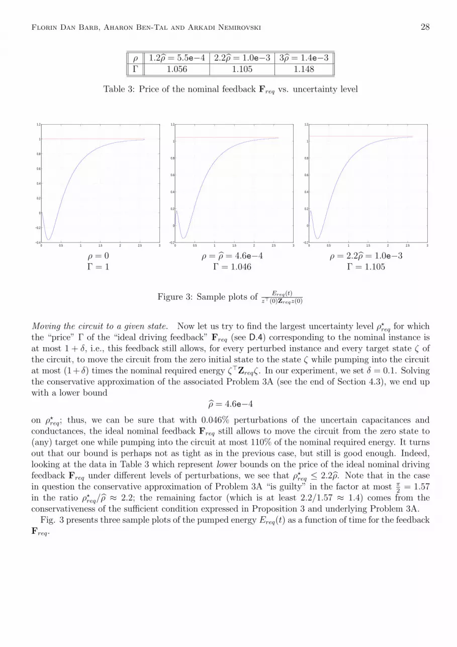
ρ 1.2ρ = 5.5e−4 2.2ρ = 1.0e−3 3ρ = 1.4e−3Γ 1.056 1.105 1.148
Table 3: Price of the nominal feedback Freq vs. uncertainty level
0 0.5 1 1.5 2 2.5 3−0.4
−0.2
0
0.2
0.4
0.6
0.8
1
1.2
0 0.5 1 1.5 2 2.5 3−0.2
0
0.2
0.4
0.6
0.8
1
1.2
0 0.5 1 1.5 2 2.5 3−0.2
0
0.2
0.4
0.6
0.8
1
1.2
ρ = 0Γ = 1
ρ = ρ = 4.6e−4Γ = 1.046
ρ = 2.2ρ = 1.0e−3Γ = 1.105
Figure 3: Sample plots of Ereq(t)
z>(0)Zreqz(0)
Moving the circuit to a given state. Now let us try to find the largest uncertainty level ρ?req for whichthe “price” Γ of the “ideal driving feedback” Freq (see D.4) corresponding to the nominal instance isat most 1 + δ, i.e., this feedback still allows, for every perturbed instance and every target state ζ ofthe circuit, to move the circuit from the zero initial state to the state ζ while pumping into the circuitat most (1 + δ) times the nominal required energy ζ>Zreqζ. In our experiment, we set δ = 0.1. Solvingthe conservative approximation of the associated Problem 3A (see the end of Section 4.3), we end upwith a lower bound
ρ = 4.6e−4
on ρ?req; thus, we can be sure that with 0.046% perturbations of the uncertain capacitances andconductances, the ideal nominal feedback Freq still allows to move the circuit from the zero state to(any) target one while pumping into the circuit at most 110% of the nominal required energy. It turnsout that our bound is perhaps not as tight as in the previous case, but still is good enough. Indeed,looking at the data in Table 3 which represent lower bounds on the price of the ideal nominal drivingfeedback Freq under different levels of perturbations, we see that ρ?req ≤ 2.2ρ. Note that in the casein question the conservative approximation of Problem 3A “is guilty” in the factor at most π
2= 1.57
in the ratio ρ?req/ρ ≈ 2.2; the remaining factor (which is at least 2.2/1.57 ≈ 1.4) comes from theconservativeness of the sufficient condition expressed in Proposition 3 and underlying Problem 3A.
Fig. 3 presents three sample plots of the pumped energy Ereq(t) as a function of time for the feedbackFreq.

Florin Dan Barb, Aharon Ben-Tal and Arkadi Nemirovski 29
1
1
2
3
4
5
Figure 4: 5 masses linked by elastic springs
5.2 Linear-Quadratic case
Consider the mechanical system shown on Fig. 4; it consists of 5 material points in a 2D plane linkedwith each other by elastic springs as shown on the figure; the points can slide without friction alongthe respective axes 01,...,05. The nominal data for the system are given in Table 4. The system is
Point MassDistance to the origin
at equilibriumSpring Rigidity
1 0.5093 0.8034 1 - 2 1.4612 0.9107 0.7430 2 - 3 1.3693 0.7224 0.9456 3 - 4 1.0884 0.8077 0.8810 4 - 5 1.2035 0.8960 0.7282 5 - 1 1.468
Table 4: The nominal data
controlled by two external forces acting at the masses 1 and 5. The first 5 components of the statevector are the shifts xi of the points from their equilibrium positions along the lines of motion, andthe next 5 components are the linear velocities xi of the points; these velocities are the outputs of thesystem. With respect to these states, the dynamical system in question is
ddt
[xx
]=
[I5
−M−1E
] [xx
]+Bu,
y = x,(56)
where M is the diagonal matrix with the masses m(i) of the points as the diagonal entries, E is thestiffness matrix readily given by the rigidities of the springs and the equilibria positions of the points,and B is the 10 × 2 matrix with two nonzero entries B5,1 = m−1(1) and B10,2 = m−1(5). Here is the
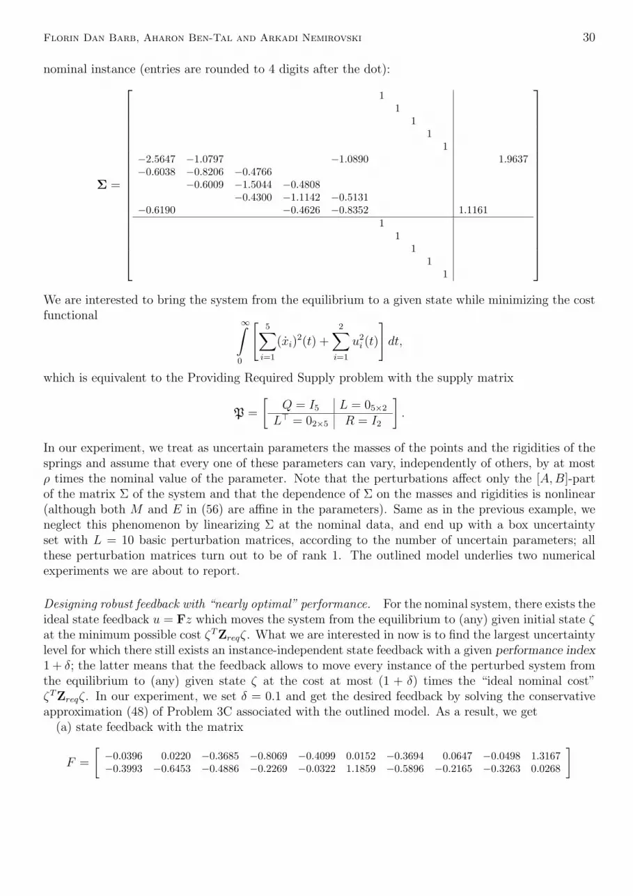
Florin Dan Barb, Aharon Ben-Tal and Arkadi Nemirovski 30
nominal instance (entries are rounded to 4 digits after the dot):
Σ =
11
11
1−2.5647 −1.0797 −1.0890 1.9637−0.6038 −0.8206 −0.4766
−0.6009 −1.5044 −0.4808−0.4300 −1.1142 −0.5131
−0.6190 −0.4626 −0.8352 1.11611
11
11
We are interested to bring the system from the equilibrium to a given state while minimizing the costfunctional ∞∫
0
[5∑i=1
(xi)2(t) +
2∑i=1
u2i (t)
]dt,
which is equivalent to the Providing Required Supply problem with the supply matrix
P =
[Q = I5 L = 05×2
L> = 02×5 R = I2
].
In our experiment, we treat as uncertain parameters the masses of the points and the rigidities of thesprings and assume that every one of these parameters can vary, independently of others, by at mostρ times the nominal value of the parameter. Note that the perturbations affect only the [A,B]-partof the matrix Σ of the system and that the dependence of Σ on the masses and rigidities is nonlinear(although both M and E in (56) are affine in the parameters). Same as in the previous example, weneglect this phenomenon by linearizing Σ at the nominal data, and end up with a box uncertaintyset with L = 10 basic perturbation matrices, according to the number of uncertain parameters; allthese perturbation matrices turn out to be of rank 1. The outlined model underlies two numericalexperiments we are about to report.
Designing robust feedback with “nearly optimal” performance. For the nominal system, there exists theideal state feedback u = Fz which moves the system from the equilibrium to (any) given initial state ζat the minimum possible cost ζTZreqζ. What we are interested in now is to find the largest uncertaintylevel for which there still exists an instance-independent state feedback with a given performance index1 + δ; the latter means that the feedback allows to move every instance of the perturbed system fromthe equilibrium to (any) given state ζ at the cost at most (1 + δ) times the “ideal nominal cost”ζTZreqζ. In our experiment, we set δ = 0.1 and get the desired feedback by solving the conservativeapproximation (48) of Problem 3C associated with the outlined model. As a result, we get
(a) state feedback with the matrix
F =
[−0.0396 0.0220 −0.3685 −0.8069 −0.4099 0.0152 −0.3694 0.0647 −0.0498 1.3167−0.3993 −0.6453 −0.4886 −0.2269 −0.0322 1.1859 −0.5896 −0.2165 −0.3263 0.0268
]

Florin Dan Barb, Aharon Ben-Tal and Arkadi Nemirovski 31
which is slightly different from the ideal nominal feedback
F =
[−0.0281 0.0289 −0.4196 −0.8948 −0.4551 0.0063 −0.3897 0.0628 −0.0558 1.3826−0.4467 −0.7133 −0.5466 −0.2423 −0.0311 1.2269 −0.6375 −0.2570 −0.3520 0.0111
]
and(b) the “safe” uncertainty level ρ = 0.0048 which is a lower bound on the optimal value ρ?3C in
Problem 3C.What we know about F and ρ from their origin is that
• The performance index of the state feedback u = Fz is no worse than 1 + δ, provided that thelevel of perturbations does not exceed 0.48% (which is our ρ). Note that this statement remainstrue even for dynamical perturbations;
• The true optimal value ρ?3C in Problem 3C is at most π2
times larger than ρ (see Proposition 8;note that our basic perturbation matrices are of rank 1, so that the quantity µ in (50) equals 2by item C of Section 4.6).
What we are interested in now is how conservative are our results, specifically, what is the actualvalue of the ratio ρ?3C/ρ. An even more important question is as follows. The optimal value ρ?3C ofProblem 3C is itself no more than a lower bound on the supremum ρ? of those perturbation levelsfor which there still exists a state feedback with performance index 1 + δ = 1.1 (since what underliesProblem 3C is no more than a sufficient condition for good performance under uncertainty). Howlarge is the ratio ρ?/ρ, or, in other words, how far is the robustness of our feedback F from the “ideal”robustness compatible with the prescribed performance index 1.1? It turns out that the answers tothese questions are quite assuring. Indeed, looking at a large enough number of randomly perturbedinstances with different perturbation levels and computing the required supply for these instances,one can find out that already at the perturbation level 1.2ρ = 0.0058 there exist perturbed instancesΣ and target states ζ such that Σ cannot be moved from the equilibrium to the state ζ at the cost≤ 1.1ζTZreqζ. It follows that
ρ?3C ≤ ρ? < 1.2ρ,
which is much better than we could expect.
Lyapunov stability analysis. Here we use the data yielded by the previous experiment for illustratinganother application of the proposed approach, namely, estimating the level of perturbations whichkeep the closed loop system stable. This problem was the subject of Example 4 in Section 3.1, whereit was shown that the problem can be posed as the one of finding the supremum of those uncertaintylevels for which all perturbed instances of the system share a common dissipativity certificate. As oursample closed loop system, we used the outlined mechanical system equipped with the state feedbackF found in the previous experiment. Our uncertainty model for the matrix
A = A+BF
of the closed loop system is as follows: we use the aforementioned “physical” model of perturbations in[A,B] and assume, in addition, that the entries in F also are subject to perturbations. Since we haveno physical model of the controller, we assume that the entries Fij in F can vary, independently of eachother (and independently of the perturbations in [A,B]), in the intervals [F c
ij−ρ|F cij|, F c
ij+ρ|F cij|], where
ρ is the uncertainty level, and F cij are the “nominal” values as computed in the previous experiment.
As in the previous cases, we linearized the dependence of A on the perturbations, thus arriving at abox model of perturbations in the matrix of the closed loop system. Then we solved the conservative

Florin Dan Barb, Aharon Ben-Tal and Arkadi Nemirovski 32
approximation (31) of Problem 1 associated with system (14) and the supply matrix (15). Since wewere interested solely in the stability of the closed loop system under perturbations, and did not careof any kind of performance, we looked for the common dissipativity certificate Z in a pretty wide“matrix interval” I = {Z : 10−7Z � Z � Z}, which in the situation of Example 4 basically meansthat we do not impose restrictions on Z except for being positive definite.
The results of our experiment are as follows. The solution of (31) yields a level of perturbations ρ =0.041 and a positive definite matrix Z which is a common Lyapunov stability certificate for all perturbedinstances of the matrix A of the closed loop system when the level of perturbations is ρ. Thus, we canbe sure that the closed loop system remains stable whatever are 4.1% perturbations of the physicalparameters of our mechanical system and 4.1% perturbations of the coefficient in the feedback matrix,even when these perturbations are dynamical. A natural question is how conservative is this conclusion.Note that a priory there is no reason to bee too optimistic in this respect, since the existence of acommon Lyapunov stability certificate, as a sufficient condition for stability, may be quite conservativealready by itself, and we are dealing with conservative approximation of this condition. However, theexperiment demonstrates that we are lucky: simulating about 1,000 random perturbations of the closedloop system at different uncertainty levels, it turns out that at the uncertainty level 1.6ρ = 0.065 therealready exist perturbations which make the closed loop system unstable. Thus, the closed loop systemdefinitely survives perturbations not exceeding 4.1% and can be crushed by 6.5%-perturbations; inreality, such an accuracy of predicting the critical level of perturbations would perhaps be consideredas not that bad.

Florin Dan Barb, Aharon Ben-Tal and Arkadi Nemirovski 33
References
[1] V. Belevitch, Classical Network Synthesis, Princeton: van Nostrand, (1968)
[2] A. Ben-Tal and A. Nemirovski, On tractable approximations of uncertain linear matrix inequalitiesaffected by interval uncertainty, to apperar in SIAM J. Optimization, (2001).
[3] A. Ben-Tal, L. El Ghaoui, A. Nemirovski, Robust Semidefinite Programming, in: H. Wolkowicz,R. Saigal, L. Vandenberghe, Eds. Handbook on Semidefinite Programming, Kluwer Academic Publishers,2000.
[4] S. Boyd, L. El Ghaoui, E. Feron and V. Balakrishnan, Linear Matrix Inequalities in Systemand Control Theory, SIAM Studies in Applied Mathematics, vol. 15, (1994).
[5] L. El Ghaoui, H. Lebret, Robust solutions to least-square problems with uncertain data matrices,SIAM J. of Matrix Anal. and Appl. 18, pp.1035-1064, (1997).
[6] L. El Ghaoui, F. Oustry, H. Lebret, Robust solutions to uncertain semidefinite programs, SIAMJ. on Optimization 9, pp. 33-52, (1998).
[7] L. E. Faibusovich, Matrix Riccati inequality:existence of solutions, Systems & Control Letters 9, pp.59-64, (1987).
[8] I. Gohberg, P. Lancaster and L. Rodman, On hermitian solutions of the symmetric algebraicRiccati equation, SIAM J. Control & Optimization 24(6), pp. 1323-1334, (1986).
[9] D. Hrovat, Application of optimal control to advanced automotive suspension design, ASME Journalof Dynamic Systems, Measurement and Control 115(2), pp. 328-342, (1993).
[10] R. Kalman, On a new characterization of linear passive systems, Proc. of the 1st Allerton Conferenceon Circuit and System Theory, Monticello, pp. 456-470, (1963)
[11] A. Nemirovski, Several NP-hard problems arising in robust stability analysis, Math. Control Signal &Systems 6, pp. 99–105, (1993).
[12] A. C. M. Ran and L. Vreugdenhil, Existence and comparision theorems for algebraic Riccati equa-tions for continuous- and discrete-time systems, Linear Algebra Appl. 99, pp. 63-83 (1988).
[13] C. Scherer, The solution set to the algebraic Riccati equation and the algebraic Riccati inequality,Linear Algebra & Its Applications 153, pp. 99-122 (1991).
[14] C. Scheer and Siep Weiland, Linear Matrix Inequalities in Control, DISC3 graduate courselecture notes (downloadable at http://www.ocp.tudelft.nl/sr/personal/Scherer/lmi.pdf) version2.0, April (1999).
[15] S. Weiland, Dissipative dynamical systems in a behavioral context, Mathematical Models and Methodsin Applied Sciences 1(1), pp. 1-25, (1991).
[16] J. C. Willems, Dissipative dynamical systems, part I: General theory, Arch. Rational Mech. Anal. 45,pp. 321-351, (1971).
[17] J. C. Willems, Dissipative dynamical systems, part II: Linear systems with quadratic supply rates,Arch. Rational Mech. Anal. 45, pp. 352-393, (1971).
3http://www.disc.tudelft.nl/

Florin Dan Barb, Aharon Ben-Tal and Arkadi Nemirovski 34
[18] J. C. Willems, Least squares stationary optimal control and the algebraic Riccati equation, IEEE T.A. C. 16(6), pp. 621-634, (1971).
[19] D.C. Youla and P. Tissi, N -port synthesis via reactance extraction – Part I., IEEE Internat. Conv.Rec., Pt. 7, pp. 183-208, (1966).


