Eng. Life Sci. 2012, 12, No. 6, 603–614 603

Walid B. Hussein

Mohamed A. Hussein

Thomas Becker

Group of (Bio-)ProcessTechnology and Process AnalysisFaculty of Life ScienceEngineering, TechnischeUniversität München, Freising,Germany

Research Article

Robust spectral estimation for speed of soundwith phase shift correction applied online inyeast fermentation processes

Ultrasound techniques are well suited to provide real-time characterization of bio-processes in non-invasive, non-contact, and non-destructive low-power consump-tion measurements. In this paper, a spectral analysis method was proposed to es-timate time of flight (TOF) between the propagated echoes, and its correspondingspeed of sound (USV). Instantaneous power spectrum distribution was used foraccurate detection of echo start times, and phase shift distribution for correcting theinvolved phase shifts. The method was validated by reference USV for pure water at9–30.8◦C, presenting a maximum error of 0.22%, which is less than that producedby the crosscorrelation method. Sensitivity analyses indicated a precision of 6.4 ×10−3% over 50 repeated experiments, and 0.11% over two different configurations.The method was competently implemented online in a yeast fermentation process,and the calculated USV was combined with temperature and nine signal features inan artificial neural network. The network was designed by back propagation algo-rithm to estimate the instantaneous density of the fermentation mixture, producinga maximum error of 0.95%.

Keywords: Fermentation monitoring / Phase-shift correction / Speed of sound / Time of flight /Ultrasound measurement

Received: October 1, 2011; revised: May 1, 2012; accepted: June 15, 2012

DOI: 10.1002/elsc.201100183

Supporting informationavailable online

1 Introduction

Ultrasound sensors are powerful tools that effectively addressthe problem of performing non-contact and non-invasive de-termination of process variables, from the viewpoint of perfor-mance and cost [1]. Ultrasound has advantages over other tra-ditional analytical techniques because measurements are rapid,non-destructive, precise, fully automated, and might be per-formed either in laboratory or online [2]. The ultrasound sensorproduces a pulse or burst signal to measure the required ultra-sound characteristics with low power consumption.

Therefore, ultrasound sensor systems open in-line applica-tions in many processes for many substances such as productcharacterization in the food, chemical, pharmaceutical andpetrol industries, control of sewage treatment, or polymeriza-tion processes, and monitoring of chemical etching [3]. More-over, typical industrial applications of ultrasound for concen-tration measurement and process monitoring include those of

Correspondence: Walid B. Hussein (whussein@wzw.tum.de),Group of (Bio-)Process Technology and Process Analysis, Faculty ofLife Sciences Engineering, Wissenschaftszentrum Weihenstephan,Weihenstephaner Steig 20, 85354 Freising, Germany.

chemical and pharmaceutical industry (polymerization, paints,and waste water treatment), food industry (beverage, dairy, andstarch production), and biotechnology (fermentation process,enzyme concentration) [4]. One of the widespread applicationsis the utilization of ultrasound for concentration measurementduring yeast fermentation process. The possibility of using low-intensity ultrasound to characterize such food processes was firstrealized over 60 years ago [5]; however, it is only recently thatthe full potential of the technique has been realized. There are anumber of reasons for the current interest in ultrasound mon-itoring during fermentation process. From one side, the foodindustry is becoming increasingly aware of the importance ofdeveloping new analytical techniques to study complex foodmaterials, and to monitor properties of foods during process-ing where strict protocols, issued by the FDA, be maintained toensure food purity; ultrasound techniques are ideally suited toboth of these applications. And from the other side, ultrasoundinstrumentation can be fully automated, make rapid and precisemeasurements, and can easily be adapted for online applications[6]. Unlikely, the ultrasound technology has a few limitationssuch as its sensitivity to air bubbles during the process course,and dependency of the acoustic properties on the specified sam-ple concentration.

C© 2012 Wiley-VCH Verlag GmbH & Co. KGaA, Weinheim www.els-journal.com

604 W. B. Hussein et al. Eng. Life Sci. 2012, 12, No. 6, 603–614

The two common approaches of ultrasound measurementsare the continuous wave approach and the pulse-echo approach.In the continuous wave approach, two separate transmitting andreceiving elements are used, which requires more complex hard-ware [7]. Meanwhile, the pulse-echo approach requires only onetransducer that operates alternatively between transmitting andreceiving modes. The latter approach offers a simple and low costsolution, even if it yields poorer results owing to the uncertaintyin the time domain measurement [8]. The main ultrasound pa-rameter for use in process monitoring and control is the speedof sound (USV). Once it is determined in a sample, the data canbe used in a number of ways, such as identification of liquids,concentrations of solutions, behavior of mixtures of liquids, andtwo-phase liquid systems [3]. USV is calculated by dividing thesignal path length over the estimated time of flight between thepropagated ultrasound echoes, and this estimation is consideredthe critical point of the whole measurement. Therefore, vari-ous methods have been developed to improve the time of flight(TOF) estimation accuracy. At which some of them based onthe proper design of the transmitting and/or receiving system(configuration approach) [9], on the generation of signals withgood time localization (sensor approach) [10], or on the usage ofsophisticated digital techniques (processing approach) [11–13].The first two strategies either offer simple and low cost resolu-tions with very poor results, or produce accurate estimations byrequiring complicated and expensive hardware. As a result, it isworth to examine the possibility of improving TOF estimationusing digital signal processing techniques rather than hardwareadaptation.

Two digital techniques are widely used to estimate TOF, thethreshold method, and the cross correlation method. The firstmethod detects the indices corresponding to the time instantswhen the signal amplitude crosses certain threshold, and TOFis then the interval between these two instances [14]. How-ever, the received echoes reach the threshold level sometimeafter their exact start. The second method searches for the in-stant at the relative maximum in the correlation function be-tween the first echo and the rest of the signal, and define TOFto be the interval between this instant and the start of firstecho [15].

Although the results obtained in the previous studies lead tothe practical conclusion that the cross correlation method en-sures up to 40% increase in the accuracy of TOF estimation withrespect to the threshold method, it requires a greater computa-tional cost and is highly influenced by noise spikes in the signal.Furthermore, the overall accuracy depends on the measurementof phase shift between the selected echoes, which is hardly no-ticed in the time domain and requires a spectral analysis in thefrequency domain.

The spectral representation of the ultrasound signal can beobtained by one of many common transformations algorithmsincluding Hilbert transformation, short time Fourier transform,or wavelet transform. The former algorithm is very sensitive tonoise and works powerfully only if the echoes are with mutualinterference [16]. Meanwhile, the other two algorithms are lesscomputational cost, efficient, and produce better noise rejection.

In this paper, a TOF estimation method was developedconsisting of two parts; the first is the enhancing of the ul-trasound signal to its exactly dominant frequency, through a

high-resolution spectral analysis based on short time Fouriertransform. Afterwards, start times of the first and second echoeswere detected on the generated instantaneous power spectrumdistribution. The second part is to apply a phase-shift correc-tion to the detected times by investigating the instantaneousphase-shift distribution. The proposed method was validated bythe standard reference data given for USV of demineralized wa-ter at elevated temperatures 9–30.8◦C. Sensitivity analyses werealso conducted to check the consistency and repeatability of themethod results. Finally, it was efficiently applied to calculate USVduring online yeast fermentation process, and combined withother signal features in a feed-forward artificial neural networkto estimate the mixture density.

2 Materials and methods

2.1 Experimental setups

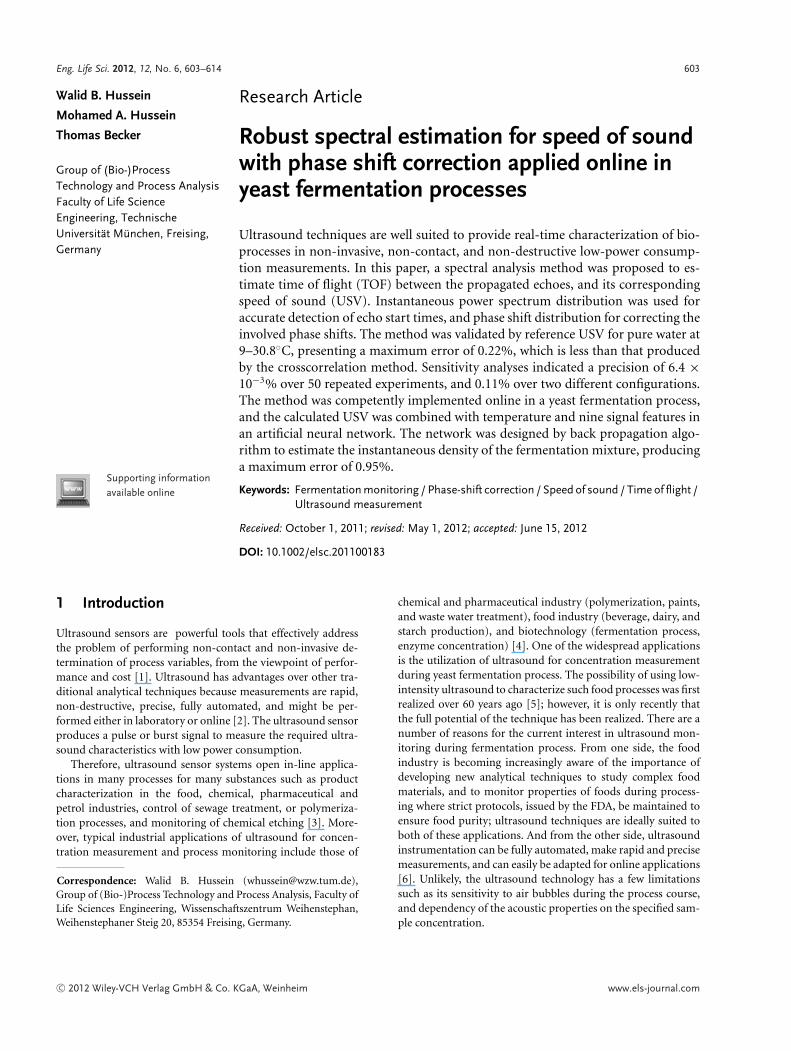
2.1.1 Hypothetical ideal pulse-echo setupOne of the commonly used arrangements in technical ultrasoundapplications is the one shown in Fig. 1A, at which ultrasoundsensor is fixed on one side of the test section, to transmit suitableenergy pulse of frequency, usually between 2 and 5 MHz. Thispulse penetrates in the test section up to the reflector side, whichreflects it back toward the sensor. Once the sensor produces thepulse, it works as a receiver to handle all the reflected and con-sequent echoes after their fully propagation into the containedmedium of the test section.

2.1.2 Real pulse-echo setupA hygienic and insulated pulse-echo setup that is widely used infood and beverage non-destructive tests was employed for thisresearch, including a stainless steel support armature to carry theinline sensors (ultrasound and temperature sensors) and a heater.The transmission-reception parts contain buffer and reflectorlids, each has 17-mm thickness, as displayed in Fig. 1B. Twodifferent nominal diameters configurations were tested for thepurpose of sensitivity analysis; the first is DN50 (50 mm) and thesecond is DN80 (80 mm). The implemented temperature sensoris PT100 (standard platinum resistance sensor) with accuracy of0.1◦C at 0◦C. The ultrasound transducer is lead zirconate titanateceramic with a resin-tungsten backing, generates a rectangular250 ns (i.e. nano-sec) impulse of 20 V amplitude and 2 MHzdominant frequency. The system was placed vertically to avoidexistence of internal air pockets.

2.1.3 Yeast fermentation setupThe bioreactor shown in Fig. 1C was employed to perform andmonitor the aerobic yeast fermentation process under brew-ing relevant conditions. The sensors are measuring turbidity,density, and ultrasound signals and were mounted inline inthe circulation pipe before the aeration jet. Moreover, the ul-trasonic sensor set up was mounted using a VARINLINE R©

coupling to insure no dead-space measurements in accor-dance with high hygienic considerations. All sensor readings arerecorded via a Beckhoff EtherCAT R© control system to a personal

C© 2012 Wiley-VCH Verlag GmbH & Co. KGaA, Weinheim www.els-journal.com

Eng. Life Sci. 2012, 12, No. 6, 603–614 Improved speed of sound calculation in yeast fermentation processes 605

Figure 1. (A) Basic pulse-echo configuration for measuring TOFbetween consequent echoes. (t) is the time axis carries informa-tion about the arrival of echoes while (y) is the distance axis carriesinformation about the path length covered by the signal. Points(A), (B), and (C) represent transmission time of main pulse andreception times for first and second echoes; respectively.(B) Layout of the pulse echo ultrasound set up consists of trans-ducer, buffer lid, sample test section of DN50 and DN80, reflectorlid, as well as attached armature with temperature sensor andheater.(C) The implemented yeast fermentation setup and its four mainitems of (1) cylindroconical vessel at which the fermentation pro-cess takes place, (2) circulation pipes, (3) gas flow panel, and (4)switch cabinet.

computer using the software package Virtual Expert R©. Fermen-tation process takes place in the stainless steel cylindroconicalvessel with a total volume of 129 L and a working volume up to60 L of wort (∼50% head space for foam formation). The in-ternal pressure was fixed at 0.9 bars to prevent foam and flowhomogenization was achieved by a centrifugal pump. An aera-tion jet “Turbo Air” R© (Co. Esau & Hueber) was introduced intothe circulation to supply yeast with oxygen. The used substrate(wort) contained approximately 10 g/100 g sugar (main compo-nents are maltose, glucose, fructose, and maltotriose) suppliedwith hops.

2.2 The proposed method

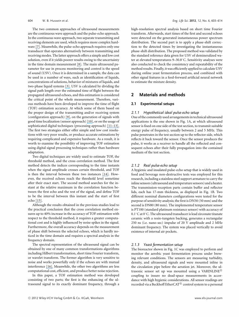
The propagation of ultrasound signals in ideal pulse-echo sys-tem (Fig. 1A), follows the one given in Fig. 2A, at which the suc-ceeded echoes can be simply detected and well defined, results instraightforward recognition of TOF and its corresponding USV.In the frequency domain, one frequency value is contained in thesignal, which is the dominant frequency fd , as illustrated by thepower spectrum distribution in Fig. 2B. Additionally, althoughthe main pulse and the received echoes are out of phase, whichmeans they have a phase difference between [0, π] radians, thereis no phase shift among the succeeding echoes, as shown in thephase-shift distribution given in Fig. 2C.

The amplitude (x) of the transmitted ultrasound signalin a medium can be mathematically modelled as a functionof its propagation time (t), as reported in [1] and given byequation (1).

x (t) = A s tme−t/u cos (2π f dt + ϕ) (1)

Where A s , fd , and ϕ are the pulse amplitude, dominant frequencyand phase shift, respectively, while m models the initial finiteslope of the pulse and u determines the final slope. Both m and uare parameters that depend on the type of ultrasound transducer.

Similarly, the amplitudes at the consequent echoes can befound for first echo, equation 2, and second echo, equation 3.

x1 (t1) = A r1 (t1)m e−t1/u cos (2π fdt1 + ϕ1) (2)

x2 (t2) = A r2 (t2)m e−t2/u cos (2πfdt2 + ϕ1) (3)

Where A r1 and A r2 are the amplitudes for first and secondechoes; respectively, t1 and t2 are the start times for firstand second echoes; respectively. ϕ1 is the phase shift of bothechoes.

Accordingly, TOF is defined as the interval between thesetwo echoes, and can be obtained directly by subtracting thetwo detected times of first and second echoes, as given inequation (4).

TOF = t2 − t1 (4)

Afterwards, USV is calculated in equation (5), by informationabout the path length of the test section (d).

USV = 2 × d

TOF(5)

C© 2012 Wiley-VCH Verlag GmbH & Co. KGaA, Weinheim www.els-journal.com

606 W. B. Hussein et al. Eng. Life Sci. 2012, 12, No. 6, 603–614

Figure 2. (A) An ideal ultrasound signal follows equation (1) withm = 2 and u = 5 × 10−7. (B) Spectrogram representation of thissignal exploring its dominant frequency at 2 MHz. (C) Phase-shiftdistribution with time at the dominant frequency showing equalphase values for the first and second echoes.

Since real applications are not provided by ideal ultrasoundsignals, recognition of the consequent echoes is not straight-forward and requires signal preprocessing. Actual transducersproduce pulses with m ≥ 0, which adds more difficulty to thetask of finding the start of an echo. Also, a real signal containsmany frequency bands beside its dominant frequency due tosensor non-perfect vibration and/or spectral leakage, at whichsome of them are mainly noise and removed by applying ap-propriate filters, while others are related to system vibration,thermodynamic parameters of the medium, or interpropaga-

tion diffraction of the echoes. Moreover, the signal is not fullydamped among the echoes intervals, and there is an interfer-ing signal produced by the attenuation and distortion betweenthe propagating sample and the reflected waves. These real-ity considerations formed two major deviations between idealand real ultrasound signals, as the real signal suffers from exis-tence of multifrequency bands instead of single-dominant fre-quency, and existence of phase shifts among the consequentechoes.

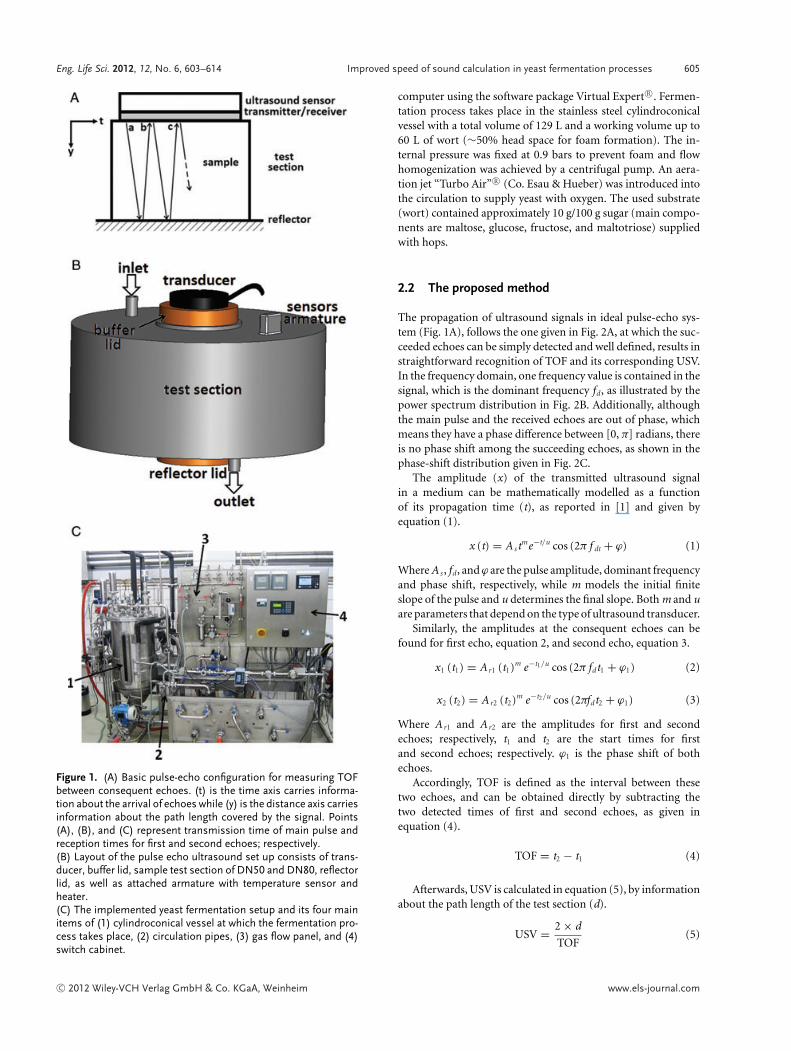
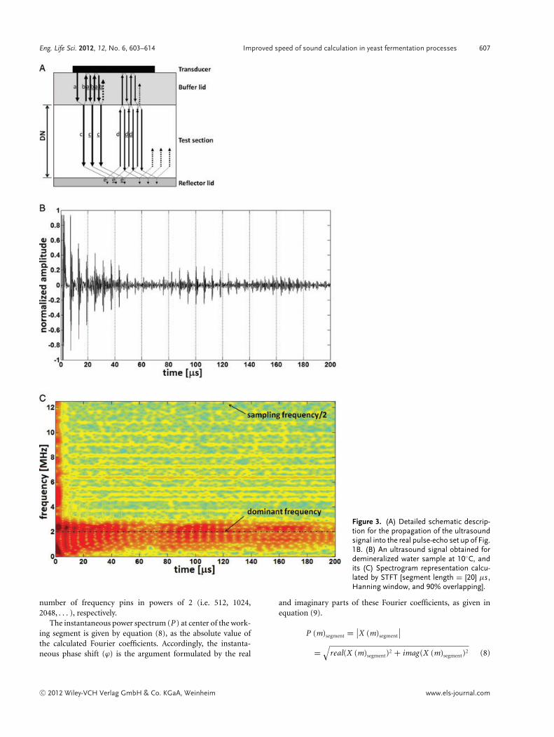
The propagation of ultrasound signal in a real pulse-echosetup (Fig. 1B), is presented in Fig. 3A. The main pulse of theultrasound signal, displayed by (arrow a), is excited at the trans-ducer and propagates downwards into the buffer lid. By ap-proaching the sample, the signal is particularly reflected towardthe sensor (arrow b), and the remaining part (arrow c) thathopefully has enough energy (depends on the buffer material)transmitted into the sample. When the transmitted part ap-proaches the reflector lid, much of the signal is reflected (arrowd) and the remaining small amount (depends on the reflectormaterial) is transmitted into the reflector lid (arrow e).

All reflections (i.e. echoes) are sensed by the transducer andmirrored back into the system to repeat the whole process (ar-rows (a, b, c, d, and e), arrows (a, b, c, d, and e), etc.). With time,most of the signal energy is dissipated into the system elements(buffer, sample, and reflector) and the echoes become weakeruntil they are fully damped.

Limiting the ultrasound signal to exactly its dominant fre-quency (fd) is a challenge due to the necessity of having high-resolution spectrogram (obtained by short time Fourier trans-form (STFT)), or scalogram (obtained by wavelet transform(WT)). However, the time resolution in WT is less at lowerfrequencies and high at higher frequencies, while it is fixed andreasonable with STFT (see Supporting information, Fig. S1). Thespectral analysis of ultrasound signals can also be performed byHilbert transformation, but it is very sensitive to noise and onlyused when the signal has few zero crossings.

As a result, STFT was employed in this work, because mostultrasound signals have low-dominant frequency, around 10%of the sampling frequency, and high time resolution is essentialto accurately determine TOF between arrived echoes. The sig-nal is divided into short overlapped segments; each with lengthequals 10% of the whole signal length, and 90% overlapping be-tween adjacent segments. Since Fourier transformation presentsspectral leakage for non-periodic signals, each segment is mul-tiplied by a Hanning window function, equation (6), forcing itto be periodic [17]. The windowed segment is transformed tofrequency domain by Fast Fourier Transform (FFT), equation(7), forming one vertical column in the generated spectrogram(see Supporting information, Fig. S2).

w(n) = 0.5

(1 − cos

(2πn

N − 1

))(6)

X (m)segment =N∑

n=1

x(n) × w(n − m) × e−i(2πfd )n,

m = 1, 2, 3, . . . , M (7)

Where x, X , w, N, and M are signal amplitude, resulting Fouriertransform coefficient, window function, segment length, and

C© 2012 Wiley-VCH Verlag GmbH & Co. KGaA, Weinheim www.els-journal.com

Eng. Life Sci. 2012, 12, No. 6, 603–614 Improved speed of sound calculation in yeast fermentation processes 607

Figure 3. (A) Detailed schematic descrip-tion for the propagation of the ultrasoundsignal into the real pulse-echo set up of Fig.1B. (B) An ultrasound signal obtained fordemineralized water sample at 10◦C, andits (C) Spectrogram representation calcu-lated by STFT [segment length = [20] μs ,Hanning window, and 90% overlapping].

number of frequency pins in powers of 2 (i.e. 512, 1024,2048, . . . ), respectively.

The instantaneous power spectrum (P ) at center of the work-ing segment is given by equation (8), as the absolute value ofthe calculated Fourier coefficients. Accordingly, the instanta-neous phase shift (ϕ) is the argument formulated by the real

and imaginary parts of these Fourier coefficients, as given inequation (9).

P (m)segment = ∣∣X (m)segment

∣∣=

√real(X (m)segment)2 + imag(X (m)segment)2 (8)

C© 2012 Wiley-VCH Verlag GmbH & Co. KGaA, Weinheim www.els-journal.com

608 W. B. Hussein et al. Eng. Life Sci. 2012, 12, No. 6, 603–614

ϕ (m)segment = X (m)segment

= tan−1

(imag(X (m)segment)

real(X (m)segment))

)∈ [−π, π] (9)

Where real(X (m)segment) and imag(X (m)segment) are the realand imaginary parts of the Fourier coefficient, respectively.

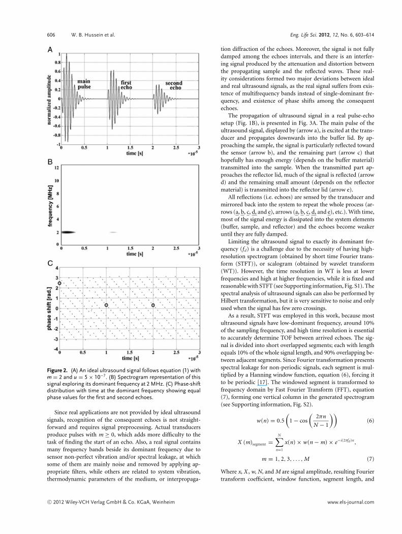
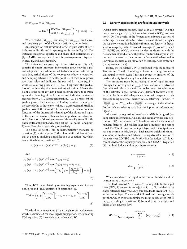
An example for real ultrasound signal in pure water at 10◦Cis shown in Fig. 3B, and its spectrogram is seen in Fig. 3C. Theinstantaneous power spectrum and phase-shift distributions at[fd = 2 MHz] are separated from this spectrogram and displayedin Figs. 4A and B, respectively.

The instantaneous power spectrum distribution (Fig. 4A)contains the most important information about how the signalis developed in the medium with details about immediate energyvariation, arrival times of the consequent echoes, attenuationand damping behavior. In depth, point 1 is at maximum powerspectrum value and indicates the start of first echo (t1, P1),while its following peaks at (1a, 1b, . . . ) represent the gradualloss of the intensity (i.e. attenuation) with time. Meanwhile,point 2 is the point at which power spectrum starts to increaseagain after damping of the first echo, and indicates the start ofsecond echo (t2, P2). Subsequent peaks (2a, 2b, 2c) represent thegradual growth for the arrivals of leading constructive chirps ofthe second echo to the sensor, while (2d, 2e,) represent the trailinggradual loss of the second echo intensity. Further echoes arefunctions of the dramatically damping of the ultrasound signalin the system; therefore, they are less important for extractionand calculation of signal parameters. Meanwhile, from Fig. 4B,phase shifts of the first and second echoes (i.e. point 1 and point2) were identified as ϕ1 and ϕ2, respectively.

The signal at point 1 can be mathematically modelled byequation (2), while at point 2, the phase shift is different fromthat at point 1, implying a modification to equation (3), whichis rewritten here as equation (10).

x1 (t1) = A r1 (t1)m e−t1/u cos (2πfdt1 + ϕ1) (2)

And

x2 (t2) = A r2 (t2)m e− t2u cos (2πfdt2 + ϕ2)

x2 (t2) = A r2 (t2)m e− t2u cos (2πfdt2 + ϕ2 − ϕ1 + ϕ1)

x2 (t2) = A r2 (t2)m e− t2u cos

(2πfd

(t2 +

[ϕ2 − ϕ1

2πfd

])+ ϕ1

)

(10)

Thus, TOF is calculated by subtracting arguments of equa-tions (10) and (2), as explained in equation (11).

TOF =(

t2 +[

ϕ2 − ϕ1

2πfd

])− t1 = t2 − t1 +

[ϕ2 − ϕ1

2πfd

]

(11)

The third term in equation (11) is the phase correction term,which is eliminated for ideal signal propagation. By estimatingTOF, equation (5) is considered to calculate USV.

2.3 Density prediction by artificial neural network

During fermentation process, yeast cells use oxygen (O2) andbreak down sugar (C6H12O6) to carbon dioxide (CO2) and wa-ter (H2O). The density of the fermentation mixture is correlatedto the sugar concentration (i.e. extract concentration), the higherthe sugar concentration the higher the mixture density. In the ab-sence of oxygen, yeast cells break down sugar to produce ethanol(C2H5OH) and (CO2), wherein the density decreases with therise of ethanol production. Therefore, mixture density is an im-portant parameter that determines the fermentation level and itslow values are used as an indication of less sugar concentration(i.e. apparent extract).

Hence, the calculated USV is combined with the measuredTemperature T and relevant signal features to design an artifi-cial neural network (ANN) for non-contact estimation of themixture density (ρest ) at any fermentation instance.

The procedure starts by extracting a list of signal featuresthrough the forms given in [18]. These features are extractedfrom the main chirp of the first echo, because it contains mostof the reflected signal information. Relevant features are se-lected to be those with adequate variation with respect to theircorresponding reference density (ρref ), satisfying [tan(20◦) ≤| ∂feature

∂ρref| ≤ tan(70◦)], where | ∂feature

∂ρref| is average of the absolute

feature-reference density variation (see Supporting information,Fig. S3).

Afterwards, a regression three-layer’s ANN is designed (seeSupporting information, Fig. S4). The input layer has one neu-ron for USV, one neuron for T, beside neurons for the selectedrelevant features. The hidden layer has a number of neuronsequal 50–60% of those in the input layer, and the output layerhas one neuron to calculate ρest . Each neuron weights the input,sums it up with a bias, and delivers it using a transfer function tothe next layer. LOGSIG transfer function (equation (12)) is ac-complished for the input layer neurons, and TANSIG (equation(13)) to both hidden and output layers neurons.

a = 1

1 + e−n(12)

a = 2

1 + e−2n− 1 (13)

Where n and a are the input to the transfer function and theneuron output, respectively.

This feed forward ANN loads N training data to the inputlayer {USV, T, relevant features}i , i = 1, . . . , N, and their asso-ciated reference density {ρref }i is compared to the resultant {ρest }i

at the output layer. The network followed back propagation al-gorithm, which tries to minimize the mean square error (MSE)in ρest , according to equation (14), by modifying the weights andbiases of the neurons [19].

MSE = 1

No. of signals

No. of signals∑i=1

(ρref − ρest

)2

i(14)

C© 2012 Wiley-VCH Verlag GmbH & Co. KGaA, Weinheim www.els-journal.com

Eng. Life Sci. 2012, 12, No. 6, 603–614 Improved speed of sound calculation in yeast fermentation processes 609

Figure 4. (A) Instantaneous power spec-trum distribution in voltage-root meansquare (Vrms) and (B) Instantaneousphase-shift distribution in radians (rad),over the signal at its dominant frequencyexploring the start and damping behaviorof each echo and differences in the phaseshifts between first and second echoes.

3 Results

The validation, sensitivity evaluation, and application of theproposed method were performed in this section (see Supportinginformation, Fig. S5).

3.1 Validation of the proposed method

Demineralized vented water was selected to validate USV val-ues obtained by the proposed method, with the reference resultsgiven in [20]. These reference data were fitted in a polynomialequation, displayed in equation (15), of six digits coefficients toensure a precision of 0.02 m/s at ambient pressure and temper-ature (T) range 0–95◦C.

USV = 1.402385 × 103 + 5.038813T − 5.799136 × 10−2T2

+ 3.287156 × 10−4T3 − 1.398845 × 10−6T4

+ 2.78786 × 10−9T5(m/s) (15)

Experiments were performed using the pulse-echo setup ofFig. 1B with DN50, along a temperature range 9–30.8◦C. Re-

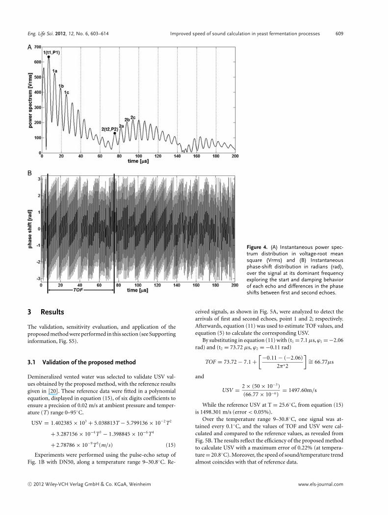
ceived signals, as shown in Fig. 5A, were analyzed to detect thearrivals of first and second echoes, point 1 and 2; respectively.Afterwards, equation (11) was used to estimate TOF values, andequation (5) to calculate the corresponding USV.

By substituting in equation (11) with (t1 = 7.1 μs, ϕ1 =−2.06rad) and (t2 = 73.72 μs, ϕ2 = −0.11 rad)

TOF = 73.72 − 7.1 +[−0.11 − (−2.06)

2π∗2

]∼= 66.77μs

and

USV = 2 × (50 × 10−3)

(66.77 × 10−6)= 1497.60m/s

While the reference USV at T = 25.6◦C, from equation (15)is 1498.301 m/s (error < 0.05%).

Over the temperature range 9–30.8◦C, one signal was at-tained every 0.1◦C, and the values of TOF and USV were cal-culated and compared to the reference values, as revealed fromFig. 5B. The results reflect the efficiency of the proposed methodto calculate USV with a maximum error of 0.22% (at tempera-ture = 20.8◦C). Moreover, the speed of sound/temperature trendalmost coincides with that of reference data.

C© 2012 Wiley-VCH Verlag GmbH & Co. KGaA, Weinheim www.els-journal.com

610 W. B. Hussein et al. Eng. Life Sci. 2012, 12, No. 6, 603–614

Figure 5. (A) Ultrasound signal obtainedin demineralized water using the pulse-echo set up of Fig. 2 with DN50 at 25.6◦C(up), and its instantaneous power spec-trum (middle) and phase-shift (bottom)distributions at the dominant frequency.(B) Speed of sound variation with temper-ature in demineralized water at 9–30.8◦C,obtained by the proposed method in com-parison to the reference data given by equa-tion 15 [20].(C) Ultrasound signal obtained for dem-ineralized water using configuration II withDN80 at 25.6◦C (top), and the instanta-neous power spectrum (middle) and phaseshift (bottom) distributions at its dominantfrequency.

3.2 Sensitivity of the proposed method

To check the reliability of the results obtained by the proposedmethod, two sensitivity analyses had been applied. The firstanalysis is related to the repeatability of the results if the mainparameters influencing the USV were fixed. Therefore, 50 ex-periments were accomplished for demineralized water at 10◦C,using the pulse-echo set up of Fig. 1B with DN50, and the re-

sulting power spectrum distributions at dominant frequency areseparated (see Supporting information, Fig. S6a).

As a result, no change in the detection of first echo through-out the 50 signals was observed and small perturbations in-fluenced the detection of second echo (see Supporting infor-mation, Fig. S6b). The average and standard deviation in thecalculated USV are 1447.28 m/s and 0.09 m/s, respectively, im-plying the consistency of the proposed method to provide reliable

C© 2012 Wiley-VCH Verlag GmbH & Co. KGaA, Weinheim www.els-journal.com

Eng. Life Sci. 2012, 12, No. 6, 603–614 Improved speed of sound calculation in yeast fermentation processes 611

Table 1. Average speed of sound obtained by the crosscorrelationand the proposed methods for demineralized water at tempera-tures of 10, 15, and 20◦C, in comparison to the reference values.USV is the average speed of sound over 50 values at the specifiedtemperature.

Temperature (◦C) USV USV USV referenceby cross by proposed (m/s)correlation (m/s) method (m/s)

10 1447.152 1447.279 1447.29115 1465.922 1465.921 1465.96220 1482.384 1482.383 1482.382

results when the dependent variable (i.e. temperature) was fixed,with a precision of ([0.09/1447.28] × 100% = 6.4 × 10−3%).Furthermore, low computational power is required to detectTOF and calculate USV for the 50 signals (around 2 s with 22.4GFlops).

The second sensitivity analysis is related to the dependencyof the results on the set up dimensions. Hence, the two nomi-nal diameters of the pulse-echo set up (i.e. DN50 and DN80)were implemented to calculate USV in pure water at T =25.6◦C. The received signals by the two setups are presentedin Figs. 5A and C, respectively, and analyzed by the proposedmethod.

For signal with DN50 setup:

TOF1 = 66.77μs, USV1 = 1497.60m/s

For signal with DN80 setup:

TOF2 = 115.6 − 8.99 +[

0.27 − (−0.58)

2π∗2

]= 106.67μs,

USV2 = 2 × (80 × 10−3)

(106.67 × 10−6)= 1499.89m/s (16)

Thus, the sensitivity of the proposed method to the configu-ration changes is:

sensitivity = standard deviation (USV1, USV2)

average (USV1, USV2)

× 100% ∼= 0.11% (17)

Alternatively, 50 experiments were executed on demineralizedwater at 10, 15, and 20◦C, and the calculated average USV arecompared to those produced by the cross correlation method andpublished in [21], as listed in Table 1. The results explore howboth methods (cross correlation, and proposed) produce highaccurate USV around T = 20◦C (error ca. 0.1 × 10−3%). Thisaccuracy is less at lower temperature, for the cross correlationmethod (error ca. 9.6 × 10−3%), and for the proposed method(error ca. 0.82 × 10−3%).

3.3 Monitoring of yeast fermentation process

Fermentation process is one of the most important processesduring malt production, due to its continuous biomixturechange along the period of process, which ends in many pro-gressions up to days. Yeast fermentation is considered to be fourmixtures process consisting of yeast, extract, water, and carbondioxide. As fermentation proceeds, density and refractive indexfall rapidly and USV gradually rises [3]. Therefore, the ultra-sound measurement becomes nearly independent of the degreeof fermentation making it suitable for continuous inline moni-toring of the process original gravity [22].

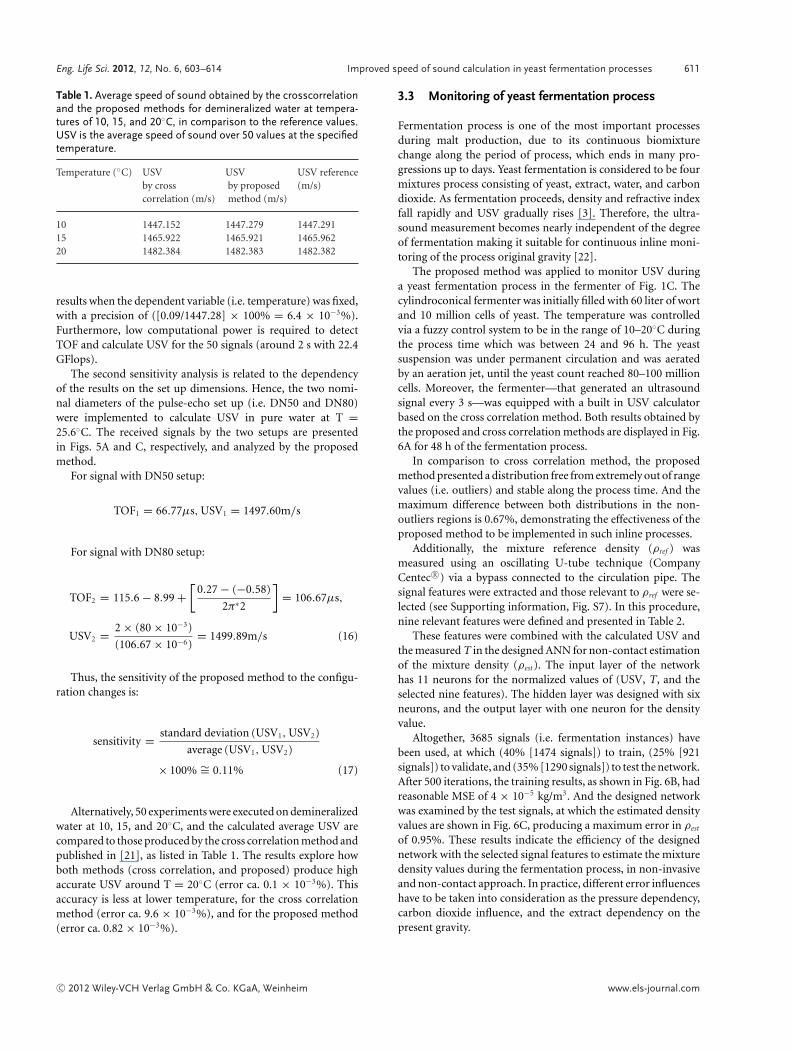
The proposed method was applied to monitor USV duringa yeast fermentation process in the fermenter of Fig. 1C. Thecylindroconical fermenter was initially filled with 60 liter of wortand 10 million cells of yeast. The temperature was controlledvia a fuzzy control system to be in the range of 10–20◦C duringthe process time which was between 24 and 96 h. The yeastsuspension was under permanent circulation and was aeratedby an aeration jet, until the yeast count reached 80–100 millioncells. Moreover, the fermenter—that generated an ultrasoundsignal every 3 s—was equipped with a built in USV calculatorbased on the cross correlation method. Both results obtained bythe proposed and cross correlation methods are displayed in Fig.6A for 48 h of the fermentation process.

In comparison to cross correlation method, the proposedmethod presented a distribution free from extremely out of rangevalues (i.e. outliers) and stable along the process time. And themaximum difference between both distributions in the non-outliers regions is 0.67%, demonstrating the effectiveness of theproposed method to be implemented in such inline processes.

Additionally, the mixture reference density (ρref ) wasmeasured using an oscillating U-tube technique (CompanyCentec R©) via a bypass connected to the circulation pipe. Thesignal features were extracted and those relevant to ρref were se-lected (see Supporting information, Fig. S7). In this procedure,nine relevant features were defined and presented in Table 2.

These features were combined with the calculated USV andthe measured T in the designed ANN for non-contact estimationof the mixture density (ρest ). The input layer of the networkhas 11 neurons for the normalized values of (USV, T, and theselected nine features). The hidden layer was designed with sixneurons, and the output layer with one neuron for the densityvalue.

Altogether, 3685 signals (i.e. fermentation instances) havebeen used, at which (40% [1474 signals]) to train, (25% [921signals]) to validate, and (35% [1290 signals]) to test the network.After 500 iterations, the training results, as shown in Fig. 6B, hadreasonable MSE of 4 × 10−5 kg/m3. And the designed networkwas examined by the test signals, at which the estimated densityvalues are shown in Fig. 6C, producing a maximum error in ρest

of 0.95%. These results indicate the efficiency of the designednetwork with the selected signal features to estimate the mixturedensity values during the fermentation process, in non-invasiveand non-contact approach. In practice, different error influenceshave to be taken into consideration as the pressure dependency,carbon dioxide influence, and the extract dependency on thepresent gravity.

C© 2012 Wiley-VCH Verlag GmbH & Co. KGaA, Weinheim www.els-journal.com

612 W. B. Hussein et al. Eng. Life Sci. 2012, 12, No. 6, 603–614

Figure 6. (A) USV distribution between the 16th and 64th h of fer-mentation, obtained by the proposed method (in solid black) andthe built-in crosscorrelation-based calculator of the fermenter (indashed gray), which suffers from many outliers along the processtime. (B) ANN training results for 1474 signals after 500 itera-tions with MSE of 4 × 10−5 kg/m3 between the estimated andreference densities of the fermentation mixture. (C) ANN testingresults for 1290 wherein maximum error between the estimatedand reference densities is 0.95%.

4 Concluding remarks

Ultrasound signal has the ability to interrogate fluids and densemixtures in a non-destructive way, which makes it an idealmethod for characterizing and process monitoring during foodproduction. The two widely used methods to estimate TOF ofan ultrasound signal—which is the most important parameterfor USV determination and further analysis—are threshold andcross correlation methods. However, the first method showedconsiderable deviations that are mainly caused by high varia-tions of the echo amplitudes, while the second method helderror due to inaccurate determination of the start of the secondecho, since other chirps may have higher correlation coefficientwith the first echo.

In this paper, a USV estimation method based on the spec-tral analysis of pulse-echo ultrasound signal at its dominantfrequency was presented, as well as a correction for the phaseshift between the first and following echoes. To assure high timeresolution, short time Fourier transform was applied to performspectral transformation of the time domain signals.

Despite of the high-resolution Fourier transform required,the computational time is still within that taken by the crosscorrelation method, because only the small region of the spec-trogram around the dominant frequency is considered, avoidingfurther calculations at other frequencies.

The method was validated by experiments in demineralizedwater at different temperatures in comparison to the cross corre-lation method. Two sensitive analyses were applied for the pro-posed method, proving its tendency to produce identical resultsif the experiment is repeated with precision of 6.4 × 10−3%,and a sensitivity of 0.11% to changes in the pulse-echo setupdimensions. The proposed method was applied to automati-cally determine online USV in yeast fermentation process witha maximum error of 0.67%. Afterwards, USV was combinedwith temperature and nine signal features in an artificial neuralnetwork to estimate the instantaneous density of the fermenta-tion mixture, producing a maximum error of 0.95%.

Although the first and second echoes were handled to cal-culate TOF for all experiments, subsequent echoes may also beused. However, the first and second echoes are qualitatively thebest selection since they are least corrupted by any destructiveissues during signal propagation.

In general, results of the proposed method, in comparison tothose given by cross correlation method, showed how it can bepowerfully applied for ultrasound measurement in food prod-ucts. Moreover, the results can be improved if higher resolutionspectral analysis is applied, with higher overlapping percent-age, less frame length, and optimum selection of the windowfunction.

In bioprocess, changes in the precision of temperature mea-surements should be well considered. The implemented PT100temperature sensor has high accuracy (0.1◦C at 0◦C), low drift,and with resistance rate of 0.385 ohm/◦C. Using sensors withhigher rates allow obtaining higher resolution. For calibration, avoltage meter was applied to adjust the resistance value for an ex-actly well-known reference temperature. However, the precisionof the temperature measurement is reduced slightly at highertemperatures, since it becomes difficult to prevent contamina-tion of the platinum wire. The precision is also degraded due to

C© 2012 Wiley-VCH Verlag GmbH & Co. KGaA, Weinheim www.els-journal.com

Eng. Life Sci. 2012, 12, No. 6, 603–614 Improved speed of sound calculation in yeast fermentation processes 613

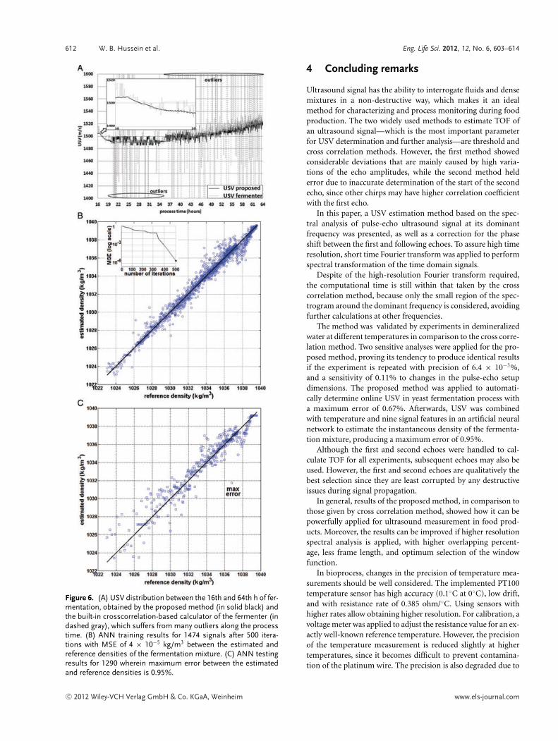
Table 2. Relevant features with respect toρref . Wherepmf , x, N, and M are probability mass function, signal amplitude, segment length, andnumber of frequency pins; respectively. X is the resulting Fourier coefficient (equation (7)).

Feature Equation

Spectral centroid∑M

m=1 m.|X (m)|∑Mm=1|X (m)|

Spectral spreadM∑

m=1(m − spectral centroid)2 × pmf (m) , pmf (m) = |X (m)|∑M

m=1|X (m)|

Spectral kurtosis∑M

m=1(m−spectral centroid)4×pmf (m)(spectral spread)2

Temporal and spectral energyN∑

n=1(x(n))2 &

M∑m=1

|X (m)|2

Temporal and spectral crest factor max(|x(n)|)1N

∑Nn=1|x(n)| & max(|X (m)|)

1M

∑Mm=1|X (m)|

Temporal and spectral entropy −N∑

n=1

( |x(n)|∑Nn=1|x(n)|

)2ln

( |x(n)|∑Nn=1|x(n)|

)2& −

M∑m=1

pmf (m) × ln(pmf (m)

)

the self-heating of the sensor as a result of the power applied toit. Further errors rise during temperature transients because thesensor may not respond to changes fast enough.

Practical application

The proposed method for estimating speed of soundpropagation of ultrasound signals can be applied in non-destructive tests to check mediums quality and variations.In particular, monitoring of fermentation processes can beperformed successfully in non-contact, non-invasive ap-proaches. Furthermore, the combination of the estimatedspeed of sound with other signal features are intended toapproximate online the important and non-sensed processvariables such as mixture density, which thereafter deter-mines the fermentation level and indicates the amount ofthe remaining sugar.

All measurements were performed in the laboratory of Chair ofBrewing and Beverage Technology, Technical University of Munich,Freising, Germany.

The authors have declared no conflict of interest.

Nomenclature

A s [Voltage] Pulse amplitudefd [Hz] Dominant frequencym Initial finite slope of the pulseu Final finite slope of the pulseA r1 [Voltage] Amplitude on the first echoA r2 [Voltage] Amplitude on the second echoTOF [s] Time of flightUSV [m/s] Speed of soundd [m] Path length through the test sectiont1 [s] Detected time for the start of first echot2 [s] Detected time for the start of second echo

ADC Analogue-to-digital converted signalamplitude

DN [m] Nominal diameterFFT Fast Fourier transformSTFT Short time Fourier transformWT Wavelet transformfs [Hz] Sampling frequencyx [Voltage] Signal amplitudeX Fourier transform coefficientw Hanning window functionN Number of segment samplesM Number of frequency pinsP [Vrms] Power spectrumP1 [Vrms] Power spectrum at the start of first

echoP2 [Vrms] Power spectrum at the start of second

echoT [◦C] TemperatureANN Artificial neural networkMSE Mean square error

a Neuron activation functionpmf Probability mass function

Greek lettersϕ [rad] Phase shiftϕ1 [rad] Phase shift at the start of first echoϕ2 [rad] Phase shift at the start of second echoρref [kg/m3] Reference density of the fermentation

mixtureρest [kg/m3] Estimated density of the fermentation

mixture

5 References

[1] Andria, G., Attivissimo, F., Giaquinto, N., Digital signal pro-cessing techniques for accurate ultrasound sensor measure-ment. Measurement 2001, 30, 105–114.

[2] Dolatowski, Z. J., Stadnik, J., Stasiak, D., Applications of ultra-sound in food technology. Acta Sci. Pol. Technol. Aliment. 2007,6(3), 89–99.

C© 2012 Wiley-VCH Verlag GmbH & Co. KGaA, Weinheim www.els-journal.com

614 W. B. Hussein et al. Eng. Life Sci. 2012, 12, No. 6, 603–614

[3] Hauptmann, P., Lucklum, R., Puettmer, A., Henning, B., Ul-trasonic sensors for process monitoring and chemical analysis:state of the art and trends. Sensors and Actuators A 1998, 67,32–48.

[4] Henning, B., Rautenberg, J., Process monitoring using ultra-sonic sensor systems. Ultrasonics 2006, 44, 1395–1399.

[5] Bamberger, J., Bond, L., Greenwood, M., Ultrasonic measure-ments for on-line real-time food process monitoring. Proceed-ing of 6th Conference on Food Engineering AIChE, Texas, USA,1999, pp. 1–4.

[6] Mason, T. J., Sonochemistry and sonoprocessing: the link, thetrends and (probably) the future. Ultrason. Sonochem. 2003,10, 175–179.

[7] Cheeke, J. D., Fundamentals and Applications of Ultra-sound Waves. First edition, CRC press LLC, USA 2002, 39–122.

[8] Guening, F., Varlan, M., Eugene, C., Dupuis, P., Accurate dis-tance measurement by an autonomous ultrasonic system com-bining time-of-flight and phase-shift methods. IEEE Trans.Instr. Meas. 1997, 46(6), 1236–1240.

[9] Schoeck, T., Becker, T., Sensor array for the combined analy-sis of water sugar ethanol mixtures in yeast fermentations byultrasound. Food Control 2010, 21(4), 362–369.

[10] Hosoda, M., Takagi, K., Ogawa, H., Nomura, H. et al., Rapidand precise measurement system for ultrasonic velocity bypulse correlation method designed for chemical analysis.Japanese J. Appl. Phys. 2005, 44(5A), 3268–3271.

[11] Anderson, W. L., Jensen, C. E., Instrumentation for time-resolved measurements of ultrasound velocity deviation. IEEETrans. Instr. Meas. 1989, 38(4), 913–916.

[12] Webster, D., A pulsed ultrasonic distance measurement system

based upon phase digitizing. IEEE Trans. Instr. Meas. 1994,43(4), 578–582.

[13] Carullo, A., Ferraris, F., Graziani, S., Grimaldi, U. et al., Ul-trasonic distance sensor improvement using a two-levelneuralnetwork. IEEE Trans. Instr. Meas. 1996, 45(2), 677–682.

[14] Parrila, M., Anaya, J. J., Fritsch, C., Digital signal processingtechniques for high accuracy ultrasonic range measurements.IEEE Trans. Instr. Meas. 1991, 40(4), 759–763.

[15] Marioli, D., Narduzzi, C., Offelli, C., Petri, D. et al., Digitaltime-of-flight measurement of ultrasonic sensor. IEEE Trans.Instr. Meas. 1992, 41(1), 198–201.

[16] Duncan, M. G., Real-time analytic signal processor for ultra-sonic non-destructive testing. IEEE Trans. Instr. Meas. 1990,39(6), 1024–1029.

[17] Hussein, W. B., Hussein, M. A., Becker, T., Detection Of The redpalm weevil rhynchophorus ferrugineus using its bioacousticsfeatures. Bioacoustics 2010, 19, 177–194.

[18] Peeters, G., A large set of audio features for sound description(similarity and classification). CUIDADO project report, AES115th Convention, New York, USA 2004, pp. 3–25.

[19] Chauvin, Y., Rumelhart, D. E., Backpropagation: Theory, ar-chitecture, and applications (1st edn.), Psychology Press, NewJersey, USA 1995, 1–35.

[20] Marczak, W., Water as a standard in the measurements of speedof sound in liquids. J. Acoust. Soc. Am. 1997, 102(5). 2776–2779.

[21] Hoche, S., Hussein, W., Hussein, M. A., Becker, T., Time offlight prediction for fermentation process monitoring. Eng.Life Sci. 2011, 11(3), 1–12.

[22] Skrgatic, D. M., Mitchinson, J. C., Graham, J. A., Measurementof specific gravity during fermentation. United States Patent4959228, 1990.

C© 2012 Wiley-VCH Verlag GmbH & Co. KGaA, Weinheim www.els-journal.com