Roughening of the anharmonic Larkin model

V. H. Purrello,1, ∗ J. L. Iguain,1, † and A. B. Kolton2, ‡

1Instituto de Investigaciones Físicas de Mar del Plata (IFIMAR),Facultad de Ciencias Exactas y Naturales, Universidad Nacional de Mar del Plata,

Consejo Nacional de Investigaciones Científicas y Técnicas (CONICET),Deán Funes 3350, B7602AYL Mar del Plata, Argentina

2Centro Atómico Bariloche and Instituto Balseiro,Comisión Nacional de Energía Atómica (CNEA),

Consejo Nacional de Investigaciones Científicas y Técnicas (CONICET),Universidad Nacional de Cuyo (UNCUYO), Av. E. Bustillo 9500,

R8402AGP San Carlos de Bariloche, Río Negro, Argentina

We study the roughening of d-dimensional directed elastic interfaces subject to quenched randomforces. As in the Larkin model, random forces are considered constant in the displacement directionand uncorrelated in the perpendicular direction. The elastic energy density contains an harmonicpart, proportional to (∂xu)2, and an anharmonic part, proportional to (∂xu)2n, where u is thedisplacement field and n > 1 an integer. By heuristic scaling arguments, we obtain the globalroughness exponent ζ, the dynamic exponent z, and the harmonic to anharmonic crossover lengthscale, for arbitrary d and n, yielding an upper critical dimension dc(n) = 4n. We find a preciseagreement with numerical calculations in d = 1. For the d = 1 case we observe, however, ananomalous “faceted” scaling, with the spectral roughness exponent ζs satisfying ζs > ζ > 1 for anyfinite n > 1, hence invalidating the usual single-exponent scaling for two-point correlation functions,and the small gradient approximation of the elastic energy density in the thermodynamic limit. Weshow that such d = 1 case is directly related to a family of Brownian functionals parameterizedby n, ranging from the random-acceleration model for n = 1, to the Lévy arcsine-law problem forn = ∞. Our results may be experimentally relevant for describing the roughening of nonlinearelastic interfaces in a Matheron-de Marsilly type of random flow.

I. INTRODUCTION

The general study of elastic interfaces in random mediais relevant for understanding generic properties displayedby a variety of experimental systems, and to successfullyclassify them into universality classes [1, 2]. Disorderadds pinning, metastability, and generates macroscopi-cally rough interfaces, while the elasticity tends to flattenthem. When driven by a uniform force F , extended in-terfaces display a nontrivial zero-temperature depinningtransition from a static to a sliding regime at a thresholdvalue Fc [3, 4], while for finite temperatures a collec-tive thermally activated creep motion persists below thedepinning threshold, F < Fc [4–7]. At zero force, theinterface gets trapped in one of the many available deepmetastable states [8, 9]. In all cases, disorder inducesstatistically self-affine rough geometries in the putativesteady states.

Universality allows convenient minimalistic models tocapture the relevant disorder-elasticity interplay. Arather minimalistic, yet nontrivial model, is the one de-scribing the position of a directed elastic interface at atime t as an univalued scalar displacement field u(x, t),where x ∈ Rd, with d the internal dimension of the mani-fold (d = 0 a particle, d = 1 for a string, d = 2 for a sheet,

∗ vpurrello@ifimar-conicet.gob.ar† iguain@mdp.edu.ar‡ koltona@cab.cnea.gov.ar

etc.), D = d+ 1 being the dimension of the space. Suchelastic interfaces do not allow the formation of overhangsnor pinch-off bubbles. Specifically, we consider an elas-tic interface, subject to a pinning force g[u(x, t), x] witha given elastic energy Eel(u). If we assume a nondrivenoverdamped relaxational dynamics at zero temperature,then the equation of motion of the interface results in

∂tu(x, t) = − δEel

δu(x, t) + g[u(x, t), x]. (1)

A rather generic disorder is specified by the averageover disorder realizations of the pinning force g(x) = 0,and its spatial autocorrelation function g(x, u)g(x′, u′) =κ2δ(x−x′)∆ξ(u−u′). Here, ∆ξ(u) is some even functionof u with ξ denoting its shortest characteristic length. Ifwe choose ∆ξ(0) = 1, then κ measures the strength ofthe disorder (see, for instance, Ref. [4]).The simplest harmonic form Eel =

∫dx(c2/2)(∂xu)2,

with c2 ≥ 0 the elastic constant, leads to the cele-brated (zero-temperature) quenched Edwards-Wilkinson(QEW) equation [10]:

∂tu(x, t) = c2∂2xu+ g[u(x, t), x]. (2)

The main difficulty of Eq. (2) is the nonlinearity andheterogeneity of the pinning forces g(u, x). This has ledLarkin and coworkers [8, 11] to approach the problemperturbatively in the disorder such that, at first order,the pinning force can be simply approximated by an x-dependent but u-independent quenched random force,

arX

iv:1

812.

1043

5v3

[co

nd-m

at.d

is-n

n] 6

Mar

201

9

2

g[u(x, t), x] ≈ f(x), with

f(x) = 0, f(x)f(x′) = κ2δ(x− x′). (3)

Replacing g by f in Eq. (2), we obtain the linear equation

∂tu(x, t) = c2∂2xu+ f(x), (4)

governing the dynamics of the so-called Larkin model(LM). Since Eq. (4) is translationally invariant, bulk dis-order does not pin the interface. However, it makes theinterface evolve to a rough steady state.

In spite of its simplicity, the LM has many interestingproperties and is a fundamental model in the theory ofdisordered elastic systems. The linear Eq. (4) is knownto correctly describe the behavior of the QEW interfaces,which evolve according to the nonlinear Eq. (2), at scalessmaller than the so-called Larkin length Lc ∼ (cξ/κ)

24−d ,

for d < 4. Above Lc the LM solution crossovers to theso-called random-manifold regime. Beyond the LM de-scription, further crossovers at larger scales are still pos-sible, depending on the properties of ∆ξ(u), and also onthe drive F [4, 7, 8, 12]. In any case, the LM is relevantto estimate the fundamental physical units for express-ing the large-scale solution of the full QEW problem.Quite remarkably, Lc can be related to the macroscopiccritical depinning threshold Fc ∼ κ/L

d/2c , the elemen-

tary pinning energy barrier Uc = FcLdcξ, and the finite

size crossover to metastability [4, 8, 9]. Above Lc, inthe random-manifold regime, pinning and elastic ener-gies scale in the same way as ∼ Uc(L/Lc)θ, with θ acharacteristic exponent, and the interface global widthas ξ(L/Lc)ζ , with ζ a roughness exponent. It is worthalso noting that the LM is relevant per se if the pinningforces have a large correlation length in the direction ofinterface displacements, such that Lc is large comparedto system size. This can be achieved if ξ is very large, thesystem is elastically stiff or the disorder very weak. Suchsituations can arise experimentally, displaying a finite-size pinning crossover [13].

Interestingly, the physics of the LM is not only rele-vant for describing small length scales. Pinning forcessuch as f(x) can be also generated via coarse-grainingat large length scales L � Lc and dominate over otherforces in driven disordered elastic systems. This hap-pens if the pinning force correlator ∆ξ(u) has a peri-odicity [14]. One simple example is a QEW interface,Eq. (2), in a disordered medium with periodic boundaryconditions in the direction of displacements, and an ad-ditional driving force F . Another less trivial example,is a one-dimensional elastic chain of particles (or inter-faces) with average separation a0, driven in a completelyuncorrelated random potential [15]. Such models are of-ten used to study friction [16, 17], but the physics is alsorelevant for charge density waves depinning [14, 18]. Inthese cases, the large-scale roughness is described by thesolution of Eq. (4).

The LM being a fundamental model in the theory ofdisordered elastic systems, it is worth analyzing how their

properties change under the influence of additional phys-ically motivated terms in Eq. (4). In this paper, wefocus in the influence of anharmonic corrections to theelasticity. To motivate the introduction of such correc-tions, we note that the LM, being linear, can be easilysolved for a particular realization of f(x) in any dimen-sion d, and averages over realizations are straightforward.Much universal information can be obtained by studyingthe critical nonstationary relaxational dynamics, from aflat initial condition at the origin of displacements, i.e.,u(x, t = 0) = 0. Since this process is dominated by a sin-gle dynamical growing length-scale l(t), for long enoughtimes before global equilibration.We define the structure factor of the

manifold as S(q, t) ≡ |u(q, t)|2, whereu(q, t) = L−d/2 ∫ dx u(x, t) e−iqx is the Fourier transformof u(x, t). Using that u(q, t = 0) = 0 we get,

S(q, t) ∝ κ2

c22q

4

(1− e−c2q

2t)2. (5)

Then, the structure factor satisfies the general scalingS(q, t) ∼ q−(d+2ζ)G(q t1/z), with G(y) = y2(ζ−ζs) fory � 1, and G(y) = yd+2ζ for y � 1 [19]. In ourcase, it is easy to check that the so-called global rough-ness exponent is ζ = (4 − d)/2, and coincides with thespectral roughness exponent ζs, while the so-called dy-namical exponent, related to the growing length-scalel(t) ∼ t1/z, is z = 2. In the steady state, roughlyreached at times t such that l(t) ∼ L, S(q, t → ∞) ∼q−(d+2ζ). For an interface of size L, this gives the globalsquared width with respect to the center of mass posi-tion W 2 ≡ [u(x, t)− vcmt]2 =

∫dq S(q, t) ∼ L2ζ , with

vcm = L−d∫dxf(x) ∼ L−d/2 the finite-size residual cen-

ter of mass velocity. The interface then becomes macro-scopically self-affine, with exponent ζ. That is, the rescal-ing x′ → b x and u′ → bζ u leads to a statistically equiv-alent interface.Interestingly, in the d = 1 LM, we have ζs = ζ > 1.

This situation, which has been called the super-roughcase in Ref. [19], has a physical peculiarity. It impliesthat the harmonic elastic approximation in Eq. (4) tothe local elastic couplings must break down in the ther-modynamic limit, since W/L ∼ Lζ−1 → ∞ as L → ∞.Local elongations are thus not bounded in the thermody-namic limit. A similar situation occurs for the roughnessexponent at the depinning threshold for the driven QEWmodel, where ζ ≈ 1.25 [20, 21]. To remedy this situation,in Ref. [22] ad hoc anharmonic corrections to the elasticenergy were introduced, such that

Eel(u) =∫dx[c2

2 (∂xu)2 + c2n

2n (∂xu)2n], (6)

with n = 2, 3, 4..., and constants c2 > 0, c2n > 0. Itis worth noting that this kind of correction is Hamil-tonian, convex, and being a correction to the elasticityonly, translational invariant. In particular, note that thepresence of the anharmonic correction breaks the tilt-symmetry of the full QEW equation, since both g(u, x)

3

and the harmonic elasticity, in contrast with the (∂xu)2n

term for n > 1, are statistically invariant by the trans-formation u → u − sxα, with α denoting any of the dinternal directions and s the parameter measuring thetilt deformation.

For large n, Eq. (6) is equivalent to impose a hard-constraint to local elongations, an usual modeling of di-rected polymers [23]. The proposed nonquadratic termsucceeds to save the elastic approximation in the thermo-dynamic limit at the depinning transition of the QEWmodel, with a new (“physical”) roughness exponent ζ =ζs ≈ 0.63 for all n > 1 [7, 22]. Quite remarkably,this value is in perfect agreement with the roughness atthe depinning transition of the paradigmatic quenchedKardar-Parisi-Zhang (QKPZ) model [10], which is inher-ently a nonequilibrium effective equation that cannot bederived directly from a Hamiltonian or free energy. Theanharmonic model hence allows us to study a model witha Hamiltonian, and a well-defined equilibrium state atF = 0, which nevertheless spontaneously generates theubiquitous Kardar-Parisi-Zhang (KPZ) [24] term, whenit is driven by a force F . Thus, one may ask whetherthe breakdown of the small gradient approximation inthe elastic energy of the d = 1 Larkin model [Eq. (4)]is, similarly, protected by introducing a nonlinear elas-ticity of the form proposed in Eq. (6), and how ζ andζs would change upon its addition. Solving the resulting“anharmonic Larkin model” would also allow us to finda possibly modified Larkin length Lc and related quanti-ties, which are fundamental to estimate both the criticalforce and the crossover length to the random manifoldregime, for the anharmonic depinning model defined byEqs. (1) and (6). The depinning transition of such modelwas analyzed in Ref. [22].

Motivated by the above phenomenology, in this work,we study the Larkin model with anharmonic elasticity,for a general dimension d and n ≥ 2. We obtain theglobal roughness exponent as a function of n and d,and also describe the crossover from harmonic to anhar-monic regimes of roughness, when two terms, one withn = 1 and another with n > 1 coexist. For the speciald = 1 case, where the small elastic deformation approxi-mation is compromised, we show that, unlike the depin-ning model, the anharmonic correction is never able toreduce ζ below unity, even in the large n almost hard-constraint limit. Moreover, we show that for all n > 1the d = 1 interface displays anomalous scaling proper-ties, with ζs > ζ ≥ 1, the so-called “faceted regime” inRef. [19]. Interestingly, we show also that this anomalouscase is closely connected to an n-parameterized familyof Brownian functionals which interpolate between therandom-acceleration process for n = 1, to the arcsine lawLévy stochastic process, for n =∞. For d > 1, however,we find ζ ≤ 1.This article is organized as follows: in Sec. II we de-

scribe the anharmonic Larkin model, the observables ofinterest, and the methods. In Sec. III we derive, viaheuristic arguments, the global roughness and dynamical

x1

x2

u(x

1,x

2,t)

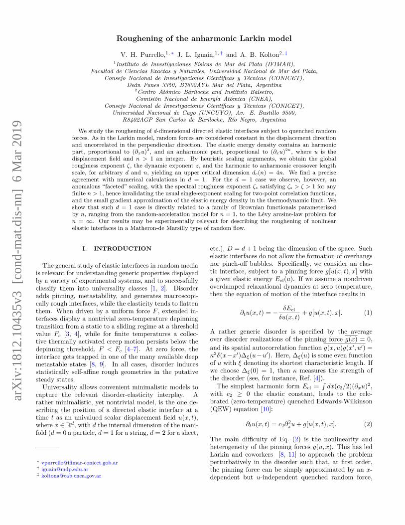
Figure 1. Schematics of the anharmonic Larkin model (ALM)for the particular d = 2 case, corresponding to a two dimen-sional interface in a three-dimensional medium. The directedinterface is described by an instantaneous scalar displacementfield in the vertical direction u(x, t) governed by Eq. (7), withx ≡ (x1, x2) the internal coordinate. The elasticity of the in-terface is nonlinear, with an elastic energy given by Eq. (6).Arrows indicate that each point x of the interface is subject toa quenched uncorrelated scalar random force f(x), describedby Eq. (3).

exponents, and also the harmonic-anharmonic crossoverlength. In Sec. IV, we numerically test these predictionsfor d = 1, solving both the relaxational dynamics of aninterface as a function of time, and the statics, for twodifferent boundary conditions. In Sec. V, we discuss therelation for the anomalous d = 1 case with a family ofBrownian functionals. Finally, in Sec. VI we present ourconclusions along with new open questions, and we sug-gest some possible applications for our results.

II. MODEL AND OBSERVABLES

We consider the anharmonic Larkin model usingEq. (1) in the Larkin approximation g(u, x)→ f(x), andEq. (6) for the elastic energy. The resulting equation ofmotion reads

∂tu(x, t) = c2∂2xu+ c2n∂x

[(∂xu)2n−1

]+ f(x), (7)

where n > 1. We will call Eq. (7) the “anharmonic Larkinmodel” (ALM). Fig. 1 schematically represents the modelfor the particular d = 2 case.Let us consider an interface of linear dimension L.

The time-dependent global width for the relaxation pro-cess W (L, t) is defined by the mean-squared fluctuationsaround the center of mass,

W 2(L, t) = 1Ld

∫dx (u− vcmt)2, (8)

4

where vcm = L−d∫dx f(x) ∼ L−d/2 [from Eq. (7)] is the

finite-size disorder-dependent but constant center of massvelocity, that may be observed for periodic or free bound-ary conditions. It is also useful to compute the time-dependent structure factor S(q, t, L), as the interface dis-placement spatial power spectrum,

S(q, t, L) = |u(q, t)|2, (9)

with u(q, t) the Fourier transform of u(x, t) as definedjust before Eq. (5).

Solving Eq. (7) from a flat initial conditionu(x, t = 0) = 0 allows us to extract several universal ex-ponents characterizing the generically expected criticalrelaxational dynamics. Such dynamics are expected tobe controlled by a single growing correlation length scale,

l(t) ∼ t1/z, (10)

with z defining the dynamical exponent. Such scaling isexpected to be valid at times larger than the microscopictime scale, but smaller than the time at which the sys-tem becomes completely correlated, i.e., when l(t) ∼ L.However, from W 2(L, t), and S(q, t, L) we can define inprinciple three different roughness exponents (z, ζ, andζs) characterizing the random geometry below l(t) [19].The global roughness exponent ζ is defined from

W (t, L) ∼ tζ/zW [L/l(t)], (11)

with

W (x) ∼{xζ if x� 1const if x� 1,

(12)

or more directly from the stationary interface width

W (t→∞, L) ∼ Lζ . (13)

Both the global ζ and the spectral ζs roughness expo-nents can be obtained from the expected scaling

S(q, t) = q−(2ζ+1) S(qt1/z

), (14)

where S(x) is the scaling function and has the generalform

S(x) ∼{x2(ζ−ζs), if x� 1x2ζ+1, if x� 1.

(15)

The stationary limit is reached when the correlationlength l(t) reaches L, at times of order Lz. Thus,

S(q) ∼ q−(2ζs+1)L2(ζ−ζs). (16)

At zero temperature, the nonstationary scaling behav-ior from Eqs. (11), (13), (14), and (15), and also thestationary scaling described by Eq. (16), are verified bythe QEW [Eq. (2)] at or above the depinning thresh-old F ≥ Fc [25, 26], and in particular by the harmonic

Larkin model [Eq. (4)] for any force, as shown in Eq. (5).In all these cases, a single growing correlation length con-trols the relaxation toward a unique self-affine stationarystate, without memory of the initial condition. Differentroughness exponents are obtained in each case. For in-stance, the d = 1 QEW equation at Fc has ζ = ζs ≈ 1.25and z ≈ 1.433 [21], while at F > Fc, it crossovers to theEdwards-Wilkinson exponents ζ = ζs = 1/2 and z = 2.The harmonic Larkin model, however, as discussed inSec. I, has ζ = ζs = (4−d)/2 and z = 2. In the followingsections, we will show that the ALM also displays thesame scaling forms, and we will obtain their exponentsζ, ζs, and z for n = 1, 2, ...,∞.

III. SCALING ARGUMENTS

The dynamical and roughness exponents of the EW,the LM and other linear models can be successfully ob-tained by simple scaling arguments (see Ref. [10] formany more relevant examples). Although such approachmay fail in general (for instance, KPZ, QKPZ, or QEWequations require renormalization group calculations in-stead), we will employ the same naive methodology forthe ALM nonlinear dynamics in Eq. (7). For simplic-ity, at first we consider only the nonlinear elastic term.Putting c2 = 0, Eq. (7) reduces to

∂tu(x, t) = c2n∂x

[(∂xu)2n−1

]+ f(x). (17)

Hence, to obtain the scaling exponents, we follow thestandard naive procedure, which consists in rescalingspace and time as

x→ x′ ≡ b x, (18)u→ u′ ≡ bζ u, (19)t→ t′ ≡ bz t. (20)

Then, making the strong assumption that the elasticityand pinning parameters are not changed by rescaling,after this transformation, Eq. (17) results in

bζ−z∂tu =

b(ζ−1)(2n−1)−1c2n∂x

[(∂xu)2n−1

]+ b−d/2f, (21)

where we have used that the random uncorrelated pin-ning forces scale as a d-dimensional random walk.We finally require the resulting equation must be in-

variant under the transformation, which leads to theFlory-like exponents,

ζ(d, n) = 4n− d4n− 2 , (22)

z(d, n) = ζ(d, n) + d

2 , (23)

for n = 1, 2, ...,∞, and general dimension d.

5

As expected, for n = 1, we recover the LM exponents,ζ = (4−d)/2 and z = 2, and the known upper critical di-mension dc(n = 1) = 4. From the prediction in Eqs. (22)and (23), it is worth noting the following:

(1) The upper critical dimension increases with n, asdc(n) = 4n.

(2) In the hard-constraint case, corresponding ton→∞, we get, for a fixed dimension d, that ζ → 1,and z → 1 + d/2.

(3) The anharmonic elastic energy density scales asL2n[ζ(d,n)−1], thus for n > 1 it is thermodynami-cally bounded only for d > 2, since ζ(d > 2, n) < 1.The d = 2 case is always marginal, ζ(d = 2, n) = 1,while the d < 2 case diverges, since ζ(d < 2, n) > 1.

(4) The spectral roughness exponent ζs does not comeout from the arguments.

If the predicted exponents are valid, then we arriveto the striking conclusion that the unbounded local dis-placements predicted for the d = 1 LM remain un-bounded, in spite of the anharmonic elasticity, for anyvalue of n. Therefore, the anharmonic correction tothe elasticity can not save the small local deformationassumption behind the gradient expansion of the elas-tic energy density, even in the n → ∞ hard-constraintlimit, in the large-size limit. This is in sharp contrast towhat happens for the d = 1 QEW equation at depinning,where the elastic approximation is saved by the very samecorrection, making the depinning roughness exponent tochange from ζdep ≈ 1.25 to the n-independent (n > 1)value ζdep ≈ 0.63 [22] [27].Let us now consider both the usual harmonic elasticity

term and the nonlinear correction together, i.e., c2 > 0and c2n > 0, for a given n > 1, in Eq. (7). In thiscase, the harmonic term should dominate the behaviorfor small distortions, so there might be an anharmoniccrossover length Lanh between two regimes of roughness,from the harmonic LM (c2 > 0, c2n = 0) to the previ-ously analyzed purely anharmonic ALM (c2 = 0, c2n > 0)universality classes. Heuristically, we can propose that,for a length-scale l > Lanh, the purely anharmonicALM displacement behaves as u ∼ uanh(l/Lanh)ζ(d,n);while for l < Lanh, we have the harmonic result u ∼(κ/c2)lζ(d,n=1) = (κ/c2)l(4−d)/2. Sharply matching thesetwo regimes at Lanh implies

uanh = κ

c2L

(4−d)/2anh . (24)

We propose that the crossover occurs when the two elas-tic energy terms are equally important, c2(uanh/Lanh)2 =(c2n/n)(uanh/Lanh)2n, thus,

uanh =(nc2

c2n

) 12(n−1)

Lanh = κ

c2L

(4−d)/2anh , (25)

which leads to the crossover length,

Lanh =(c2

κ

) 22−d

(nc2

c2n

) 1(2−d)(n−1)

. (26)

This means that, for the combined elasticities, we wouldhave, in the stationary limit of a large system L� Lanh,a crossover behavior as a function of the length-scale inthe correlation functions. For instance, the mean-squarewidth [Eq. (8)] is expected to satisfy

W 2(L, t→∞) = L2ζ(d,n=1) w(L/Lanh), (27)

with w(x) = x2[ζ(d,n>1)−ζ(d,n=1)], for x � 1; andw(x) ∼ constant, for x� 1.In the following two sections, we numerically check all

these heuristic scaling predictions, for the special d = 1case.

IV. NUMERICAL RESULTS FOR d = 1

To test the validity and robustness of the scaling pre-dictions, we have found convenient to analyze separatelythe static solution, using appropriate boundary condi-tions. With these numerical methods, we are able toaccess all the exponents ζ, ζs, and z, and the crossoverlength Lanh.

A. Static solution

We study the static geometric properties of the ALM,by solving Eq. (7) in the stationary limit, where the elas-tic and random forces exactly balance, i.e.,

c2∂2xu+ c2n∂x[(∂xu)2n−1] = −f(x). (28)

1. Global roughness exponent

Since the anharmonic term dominates the geometry atlarge length scales, we first focus on the purely anhar-monic ALM by fixing c2 = 0 in Eq. (28). This is thenstraightforward to solve:

u(x) = −∫ x

0dx′

[∫ x′

0dx′′

f(x′′)c2n

− (∂xu(0))2n−1

] 12n−1

,

(29)where we have used the particular boundary conditionu(0, t) = 0. As elastic interactions are short ranged, thisparticular boundary condition does not alter the large-scale scaling properties we are interested in.To numerically evaluate Eq. (29), we simply discretize

the d = 1 interface in segments of size δx, and performthe sums

ui = −i−1∑j=0

[j∑

k=0

fkc2n

] 12n−1

, for i > 0, (30)

6

10−2

10−1

100

102 103 104 105 106 107 108

u2 L/L2ζ(d

=1,n

)

L

n = 1n = 2n = 4n = 8n = 16

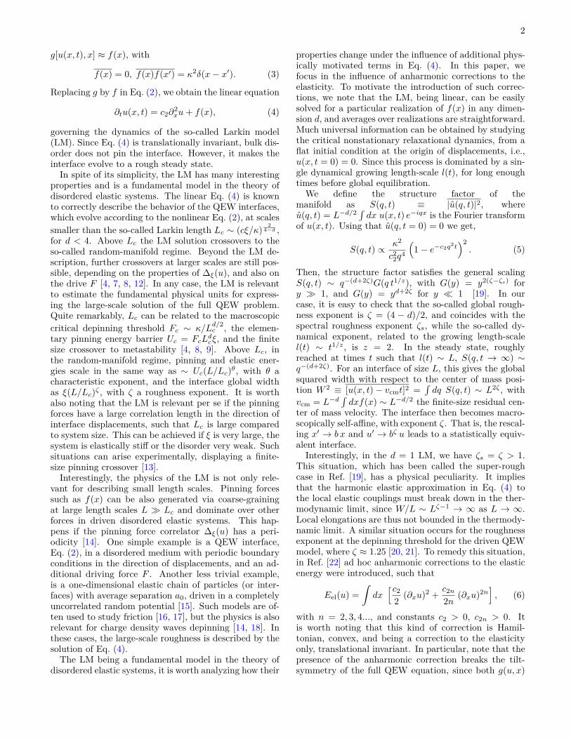
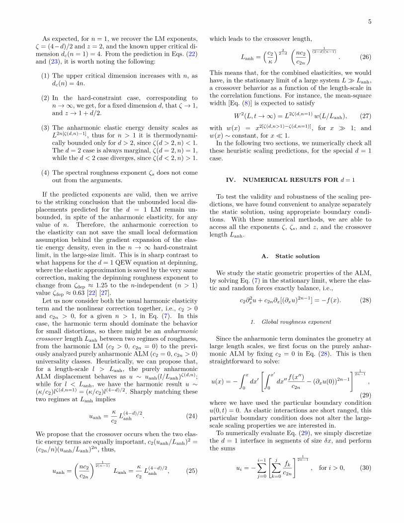
Figure 2. Disorder-averaged last-end-point squared displace-ment of a d = 1 ALM interface divided by the expected sizescaling, as a function of the system size L, using 104 samplesfor each value of n and L. Constant behavior at large L con-firms the validity of the predicted global roughness exponentζ(d = 1, n) of Eq. (22). The error bars are estimated fromthe standard deviations.

with u0 = 0 fixed, and f0 ≡ −∑Li=1 fi; taking

care of the statics of the whole polymer of size L inthe discrete description, and accounting for the term[∂xu(0)]2n−1 ∼ (u1 − u0)2n−1 = −f0/c2n in the contin-uum Eq. (29) [28]. Note that, without loss of general-ity, we have taken δx = 1 exploiting that the pinningforce is completely uncorrelated in the internal coordi-nate. We have drawn fk from a uniform distributionwith zero mean and variance κ2 = 1/12.Equation (30) can then be solved very efficiently for

large system sizes, by using parallel random number gen-erators and parallel prefix-sum algorithms implementedin massively parallel coprocessors, such as graphic cards.As the same scaling analysis leading to the prediction inEq. (22) applies to Eq. (29) or Eq. (30), regardless of thefixed-end condition u0 = 0, we expect to get ζ(d = 1, n)from the numerical evaluation of Eq. (30). Since the sys-tem is not translational invariant along x, it is convenientto directly measure the last-point scaling, for which weexpect u2

L ∼ L2ζ(d=1,n), for large enough L.In Fig. 2 we show there is an excellent agreement be-

tween predicted behavior and the obtained results forvarious values of n, for system sizes larger than around102, and up to 108 string elements.

2. Harmonic to anharmonic crossover

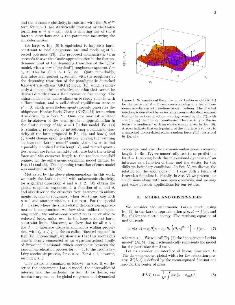
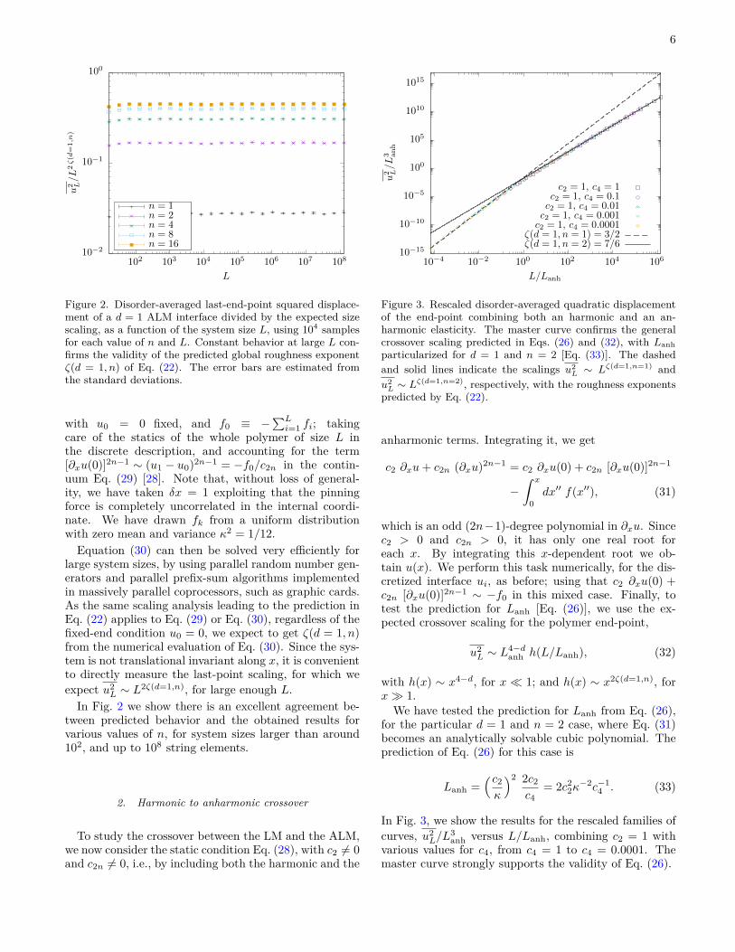
To study the crossover between the LM and the ALM,we now consider the static condition Eq. (28), with c2 6= 0and c2n 6= 0, i.e., by including both the harmonic and the

10−15

10−10

10−5

100

105

1010

1015

10−4 10−2 100 102 104 106

u2 L/L3 an

h

L/Lanh

c2 = 1, c4 = 1c2 = 1, c4 = 0.1c2 = 1, c4 = 0.01c2 = 1, c4 = 0.001c2 = 1, c4 = 0.0001

ζ(d = 1, n = 1) = 3/2ζ(d = 1, n = 2) = 7/6

Figure 3. Rescaled disorder-averaged quadratic displacementof the end-point combining both an harmonic and an an-harmonic elasticity. The master curve confirms the generalcrossover scaling predicted in Eqs. (26) and (32), with Lanhparticularized for d = 1 and n = 2 [Eq. (33)]. The dashedand solid lines indicate the scalings u2

L ∼ Lζ(d=1,n=1) andu2L ∼ L

ζ(d=1,n=2), respectively, with the roughness exponentspredicted by Eq. (22).

anharmonic terms. Integrating it, we get

c2 ∂xu+ c2n (∂xu)2n−1 = c2 ∂xu(0) + c2n [∂xu(0)]2n−1

−∫ x

0dx′′ f(x′′), (31)

which is an odd (2n−1)-degree polynomial in ∂xu. Sincec2 > 0 and c2n > 0, it has only one real root foreach x. By integrating this x-dependent root we ob-tain u(x). We perform this task numerically, for the dis-cretized interface ui, as before; using that c2 ∂xu(0) +c2n [∂xu(0)]2n−1 ∼ −f0 in this mixed case. Finally, totest the prediction for Lanh [Eq. (26)], we use the ex-pected crossover scaling for the polymer end-point,

u2L ∼ L

4−danh h(L/Lanh), (32)

with h(x) ∼ x4−d, for x � 1; and h(x) ∼ x2ζ(d=1,n), forx� 1.We have tested the prediction for Lanh from Eq. (26),

for the particular d = 1 and n = 2 case, where Eq. (31)becomes an analytically solvable cubic polynomial. Theprediction of Eq. (26) for this case is

Lanh =(c2

κ

)2 2c2

c4= 2c2

2κ−2c−1

4 . (33)

In Fig. 3, we show the results for the rescaled families ofcurves, u2

L/L3anh versus L/Lanh, combining c2 = 1 with

various values for c4, from c4 = 1 to c4 = 0.0001. Themaster curve strongly supports the validity of Eq. (26).

7

B. Dynamic Solution

To test dynamical scaling (i.e., involving the time vari-able), we have performed numerical simulations of Eq. (7)in d = 1 with periodic boundary conditions, and we haveaveraged the results over many disorder realizations. Wehave implemented this by using a spatial finite differ-ence scheme, and we have solved the resulting systemof equations following the standard Euler method. Ifthe discretization is δx, such that ui ≡ u(x = iδx), fori = 1, 2, . . . , L, then Eq. (7) can be approximated by

∂tui = c2

(δx)3 (ui+1 + ui−1 − 2ui)

+ c2n

(δx)2n+1

[(ui+1 − ui)2n−1 − (ui − ui−1)2n−1

]+ fi, (34)

with u0 ≡ uL and uL+1 ≡ u1. The d-dimensional gener-alization is straightforward. We draw the random forcesfi from a uniform distribution with zero mean and vari-ance κ2 = 1/12, and we solve Eq. (34) starting from aflat configuration ui(t = 0) = 0.

1. Time dependent structure factor

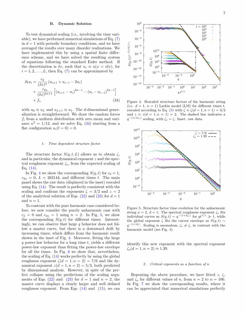
The structure factor S(q, t, L) allows us to obtain ζ,and in particular, the dynamical exponent z and the spec-tral roughness exponent ζs, from the expected scaling ofEq. (14).

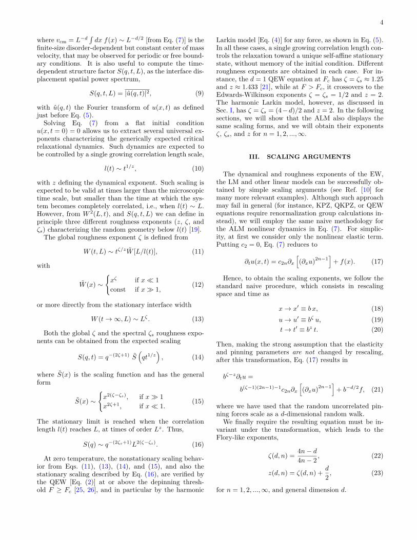
In Fig. 4 we show the corresponding S(q, t) for c2 = 1,c2n = 0, L = 262144, and different times t. The mainpanel shows the raw data (displayed in the inset) rescaledusing Eq. (14). The result is perfectly consistent with thescaling and confirms the exponents ζ = 3/2 and z = 2of the analytical solution of Eqs. (22) and (23) for d = 1and n = 1.

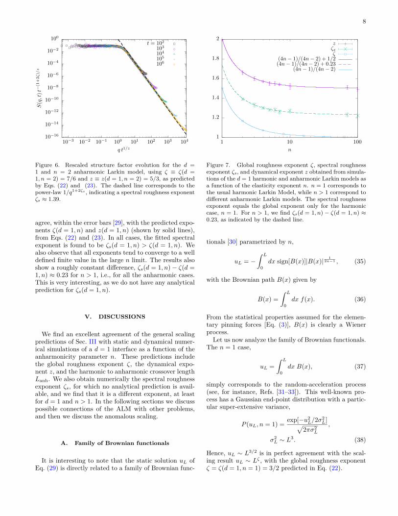
To contrast with the pure harmonic case considered be-fore, we now consider the purely anharmonic case withc2 = 0 and c2n = 1 using n = 2. In Fig. 5, we showthe corresponding S(q, t) for different times. Interest-ingly, we can observe that large q behavior does not fol-low a master curve, but there is a downward drift byincreasing times, which differs from the harmonic resultshown in the inset of Fig. 4. Moreover, fitting the largeq power-law behavior for a long time t, yields a differentpower-law exponent than fitting the power-law envelopefor all the times. In Fig. 6 we show that, nevertheless,the scaling of Eq. (14) works perfectly by using the globalroughness exponent ζ(d = 1, n = 2) = 7/6 and the dy-namical exponent z(d = 1, n = 2) = 5/3, both predictedby dimensional analysis. However, in spite of the per-fect collapse using the predictions of the scaling argu-ments of Eqs. (22) and (23) for d = 1 and n = 2, themaster curve displays a clearly larger and well definedroughness exponent. From Eqs. (14) and (15), we can

10−16

10−14

10−12

10−10

10−8

10−6

10−4

10−2

100

10−3 10−2 10−1 100 101 102 103

10−4

1001041081012

10−4 10−2 100

S(q,t)t−

(1+2ζ)/z

q t1/z

t = 102

103

104

105

106

S(q,t)

q

Figure 4. Rescaled structure factors of the harmonic string(i.e. d = 1, n = 1) Larkin model (LM) for different times t,rescaled according to Eq. (5) with ζ ≡ ζ(d = 1, n = 1) = 3/2and z ≡ z(d = 1, n = 1) = 2. The dashed line indicates aq−(1+2ζs) scaling, with ζs = ζ. Inset: raw data.

10−2

100

102

104

106

108

1010

1012

10−4 10−3 10−2 10−1 100

S(q,t)

q

ζ = 7/6ζs = 1.39

Figure 5. Structure factor time evolution for the anharmonicstring n = 2, d = 1. The spectral roughness exponent ζs fitsindividual curves as S(q, t) ∼ q−(1+2ζs) for qt1/z � 1, whilethe global exponent ζ fits the curves envelope as S(q, t) ∼q−(1+2ζ). Scaling is anomalous, ζs 6= ζ, in contrast with theharmonic model (see Fig. 4).

identify this new exponent with the spectral exponentζs(d = 1, n = 2) ≈ 1.39.

2. Critical exponents as a function of n

Repeating the above procedure, we have fitted z, ζ,and ζs for different values of n, from n = 2 to n = 100.In Fig. 7 we show the corresponding results, where itcan be appreciated that numerical simulations perfectly

8

10−16

10−14

10−12

10−10

10−8

10−6

10−4

10−2

100

10−3 10−2 10−1 100 101 102 103 104

S(q,t)t−

(1+2ζ)/z

q t1/z

t = 102

103

104

105

106

Figure 6. Rescaled structure factor evolution for the d =1 and n = 2 anharmonic Larkin model, using ζ ≡ ζ(d =1, n = 2) = 7/6 and z ≡ z(d = 1, n = 2) = 5/3, as predictedby Eqs. (22) and (23). The dashed line corresponds to thepower-law 1/q1+2ζs , indicating a spectral roughness exponentζs ≈ 1.39.

agree, within the error bars [29], with the predicted expo-nents ζ(d = 1, n) and z(d = 1, n) (shown by solid lines),from Eqs. (22) and (23). In all cases, the fitted spectralexponent is found to be ζs(d = 1, n) > ζ(d = 1, n). Wealso observe that all exponents tend to converge to a welldefined finite value in the large n limit. The results alsoshow a roughly constant difference, ζs(d = 1, n)− ζ(d =1, n) ≈ 0.23 for n > 1, i.e., for all the anharmonic cases.This is very interesting, as we do not have any analyticalprediction for ζs(d = 1, n).

V. DISCUSSIONS

We find an excellent agreement of the general scalingpredictions of Sec. III with static and dynamical numer-ical simulations of a d = 1 interface as a function of theanharmonicity parameter n. These predictions includethe global roughness exponent ζ, the dynamical expo-nent z, and the harmonic to anharmonic crossover lengthLanh. We also obtain numerically the spectral roughnessexponent ζs, for which no analytical prediction is avail-able, and we find that it is a different exponent, at leastfor d = 1 and n > 1. In the following sections we discusspossible connections of the ALM with other problems,and then we discuss the anomalous scaling.

A. Family of Brownian functionals

It is interesting to note that the static solution uL ofEq. (29) is directly related to a family of Brownian func-

1

1.2

1.4

1.6

1.8

2

1 10 100

n

zζsζ

(4n− 1)/(4n− 2) + 1/2(4n− 1)/(4n− 2) + 0.23

(4n− 1)/(4n− 2)

Figure 7. Global roughness exponent ζ, spectral roughnessexponent ζs, and dynamical exponent z obtained from simula-tions of the d = 1 harmonic and anharmonic Larkin models asa function of the elasticity exponent n. n = 1 corresponds tothe usual harmonic Larkin Model, while n > 1 correspond todifferent anharmonic Larkin models. The spectral roughnessexponent equals the global exponent only for the harmoniccase, n = 1. For n > 1, we find ζs(d = 1, n) − ζ(d = 1, n) ≈0.23, as indicated by the dashed line.

tionals [30] parametrized by n,

uL = −∫ L

0dx sign[B(x)]|B(x)|

12n−1 , (35)

with the Brownian path B(x) given by

B(x) =∫ L

0dx f(x). (36)

From the statistical properties assumed for the elemen-tary pinning forces [Eq. (3)], B(x) is clearly a Wienerprocess.Let us now analyze the family of Brownian functionals.

The n = 1 case,

uL =∫ L

0dx B(x), (37)

simply corresponds to the random-acceleration process(see, for instance, Refs. [31–33]). This well-known pro-cess has a Gaussian end-point distribution with a partic-ular super-extensive variance,

P (uL, n = 1) = exp[−u2L/2σ2

L]√2πσ2

L

,

σ2L ∼ L3. (38)

Hence, uL ∼ L3/2 is in perfect agreement with the scal-ing result uL ∼ Lζ , with the global roughness exponentζ = ζ(d = 1, n = 1) = 3/2 predicted in Eq. (22).

9

0

0.5

1

1.5

2

2.5

3

3.5

4

4.5

−1 −0.8 −0.6 −0.4 −0.2 0 0.2 0.4 0.6 0.8 1

P(uL,n

)Lζ(d

=1,n

)

uL/Lζ(d=1,n)

n = 1n = 2n = 16

n = 1024Gaussian law

Arcsine law

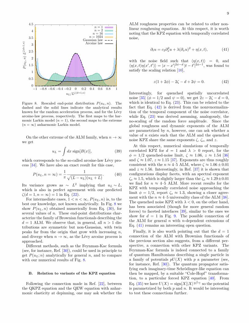
Figure 8. Rescaled end-point distribution P (uL, n). Thedashed and the solid lines indicate the analytical resultsknown for the random acceleration process, and for the Lévyarcsine-law process, respectively. The first maps to the har-monic Larkin model (n = 1), the second maps to the extreme(n =∞) anharmonic Larkin model.

On the other extreme of the ALM family, when n→∞we get

uL =∫dx sign[B(x)], (39)

which corresponds to the so-called arcsine-law Lévy pro-cess [34]. We have also an exact result for this case,

P (uL, n =∞) = 1π

1√(L− uL)(uL + L)

. (40)

Its variance grows as ∼ L2 implying that uL ∼ L,which is also in perfect agreement with our predictedζ(d = 1, n =∞) = 1 in Eq. (22).

For intermediate cases, 1 < n <∞, P (uL, n) is, to thebest our knowledge, not known analytically. In Fig. 8 weshow P (uL, n) obtained numerically from Eq. (30), forseveral values of n. These end-point distributions char-acterize the family of Brownian functionals describing thed = 1 ALM. We observe that, in general, all n > 1 dis-tributions are symmetric but non-Gaussian, with twinpeaks far from the origin that grow with increasing n,and diverge when n→∞, as the Lévy arcsine process isapproached.

Different methods, such as the Feynman-Kac formula(see, for instance, Ref. [30]), could be used in principle toget P (uL;n) analytically for general n, and to comparewith our numerical results of Fig. 8.

B. Relation to variants of the KPZ equation

Following the connection made in Ref. [22], betweenthe QKPZ equation and the QEW equation with anhar-monic elasticity at depinning, one may ask whether the

ALM roughness properties can be related to other non-linear roughening equations. At this respect, it is worthnoting that the KPZ equation with temporally correlatednoise,

∂tu = c2∂2xu+ λ(∂xu)2 + η(x, t), (41)

with the noise field such that 〈η(x, t)〉 = 0, and〈η(x, t)η(x′, t′)〉 = |x − x′|2ψ−d |t − t′|2φ−1, was found tosatisfy the scaling relation [10],

z(1 + 2φ)− 2ζ − d+ 2ψ = 0. (42)

Interestingly, for quenched spatially uncorrelatednoise [35] (φ = 1/2 and ψ = 0), we get 2z − 2ζ − d = 0,which is identical to Eq. (23). This can be related to thefact that Eq. (42) is derived from the nonrenormaliza-tion of the temporal component of the noise correlator,while Eq. (23) was derived assuming, analogously, theno-scaling of the random force amplitude. Since theglobal roughness and dynamic exponents of the ALMare parametrized by n, however, one can ask whether avalue of n exists such that the ALM and the quenchednoise KPZ share the same exponents ζ, ζs, and z.At this respect, numerical simulations of temporally

correlated KPZ for d = 1 and λ > 0 report, for theφ = 1/2 quenched-noise limit, ζ ≈ 1.06, z ≈ 1.54 [36]and ζ ≈ 1.07, z ≈ 1.15 [37]. Exponents are thus roughlyconsistent with the n ≈ 4–5 ALM, where ζ ≈ 1.06± 0.01and z ≈ 1.56. Interestingly, in Ref. [37] it is shown thatconfigurations display facets, with an spectral exponentζs ≈ 1.5, which is slightly larger than the ζs ≈ 1.29±0.01we find for n ≈ 4–5 ALM. More recent results for theKPZ with temporally correlated noise approaching thelimit φ = 1/2, report ζs ≈ 1.3, showing a closer agree-ment with the n ≈ 4–5 universality class of the ALM [38].The quenched noise KPZ with λ < 0, on the other hand,has been associated (though for more general randomforces) to faceted interfaces [39], similar to the ones weshow for d = 1 in Fig. 9. The possible connection ofthe ALM for general n with n-dependent extensions ofEq. (41) remains an interesting open question.

Finally, it is also worth pointing out that the d = 1connection of the ALM with Brownian functionals ofthe previous section also suggests, from a different per-spective, a connection with other KPZ variants. TheFeynman-Kac formula is indeed connected to a familyof quantum Hamiltonians describing a single particle ina family of potentials pU(X) with p a parameter (see,for instance, Ref. [30]). The quantum propagator satis-fying each imaginary-time Schrödinger-like equation canthen be mapped, by a suitable “Cole-Hopf” transforma-tion, to a particular forced KPZ equation [40]. FromEq. (35) we have U(X) = sign[X]|X|

12n−1 so the potential

is parametrized by both p and n. It would be interestingto test these connections further.

10

−400

−300

−200

−100

0

100

200

300

400

200 400 600 800 1000

u

x

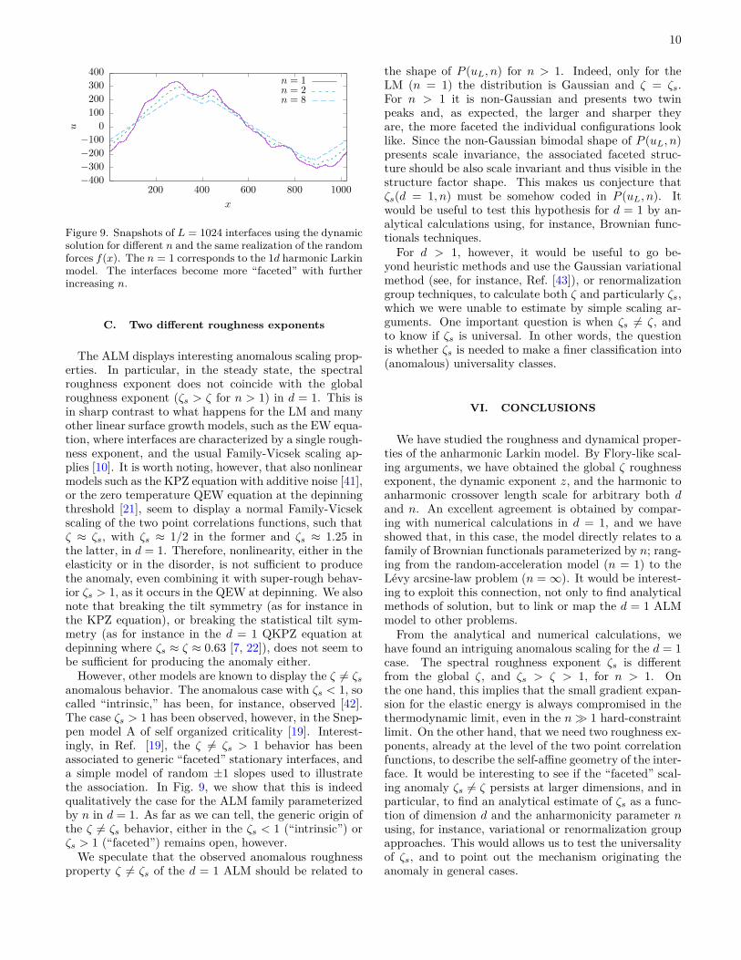
n = 1n = 2n = 8

Figure 9. Snapshots of L = 1024 interfaces using the dynamicsolution for different n and the same realization of the randomforces f(x). The n = 1 corresponds to the 1d harmonic Larkinmodel. The interfaces become more “faceted” with furtherincreasing n.

C. Two different roughness exponents

The ALM displays interesting anomalous scaling prop-erties. In particular, in the steady state, the spectralroughness exponent does not coincide with the globalroughness exponent (ζs > ζ for n > 1) in d = 1. This isin sharp contrast to what happens for the LM and manyother linear surface growth models, such as the EW equa-tion, where interfaces are characterized by a single rough-ness exponent, and the usual Family-Vicsek scaling ap-plies [10]. It is worth noting, however, that also nonlinearmodels such as the KPZ equation with additive noise [41],or the zero temperature QEW equation at the depinningthreshold [21], seem to display a normal Family-Vicsekscaling of the two point correlations functions, such thatζ ≈ ζs, with ζs ≈ 1/2 in the former and ζs ≈ 1.25 inthe latter, in d = 1. Therefore, nonlinearity, either in theelasticity or in the disorder, is not sufficient to producethe anomaly, even combining it with super-rough behav-ior ζs > 1, as it occurs in the QEW at depinning. We alsonote that breaking the tilt symmetry (as for instance inthe KPZ equation), or breaking the statistical tilt sym-metry (as for instance in the d = 1 QKPZ equation atdepinning where ζs ≈ ζ ≈ 0.63 [7, 22]), does not seem tobe sufficient for producing the anomaly either.

However, other models are known to display the ζ 6= ζsanomalous behavior. The anomalous case with ζs < 1, socalled “intrinsic,” has been, for instance, observed [42].The case ζs > 1 has been observed, however, in the Snep-pen model A of self organized criticality [19]. Interest-ingly, in Ref. [19], the ζ 6= ζs > 1 behavior has beenassociated to generic “faceted” stationary interfaces, anda simple model of random ±1 slopes used to illustratethe association. In Fig. 9, we show that this is indeedqualitatively the case for the ALM family parameterizedby n in d = 1. As far as we can tell, the generic origin ofthe ζ 6= ζs behavior, either in the ζs < 1 (“intrinsic”) orζs > 1 (“faceted”) remains open, however.

We speculate that the observed anomalous roughnessproperty ζ 6= ζs of the d = 1 ALM should be related to

the shape of P (uL, n) for n > 1. Indeed, only for theLM (n = 1) the distribution is Gaussian and ζ = ζs.For n > 1 it is non-Gaussian and presents two twinpeaks and, as expected, the larger and sharper theyare, the more faceted the individual configurations looklike. Since the non-Gaussian bimodal shape of P (uL, n)presents scale invariance, the associated faceted struc-ture should be also scale invariant and thus visible in thestructure factor shape. This makes us conjecture thatζs(d = 1, n) must be somehow coded in P (uL, n). Itwould be useful to test this hypothesis for d = 1 by an-alytical calculations using, for instance, Brownian func-tionals techniques.For d > 1, however, it would be useful to go be-

yond heuristic methods and use the Gaussian variationalmethod (see, for instance, Ref. [43]), or renormalizationgroup techniques, to calculate both ζ and particularly ζs,which we were unable to estimate by simple scaling ar-guments. One important question is when ζs 6= ζ, andto know if ζs is universal. In other words, the questionis whether ζs is needed to make a finer classification into(anomalous) universality classes.

VI. CONCLUSIONS

We have studied the roughness and dynamical proper-ties of the anharmonic Larkin model. By Flory-like scal-ing arguments, we have obtained the global ζ roughnessexponent, the dynamic exponent z, and the harmonic toanharmonic crossover length scale for arbitrary both dand n. An excellent agreement is obtained by compar-ing with numerical calculations in d = 1, and we haveshowed that, in this case, the model directly relates to afamily of Brownian functionals parameterized by n; rang-ing from the random-acceleration model (n = 1) to theLévy arcsine-law problem (n =∞). It would be interest-ing to exploit this connection, not only to find analyticalmethods of solution, but to link or map the d = 1 ALMmodel to other problems.

From the analytical and numerical calculations, wehave found an intriguing anomalous scaling for the d = 1case. The spectral roughness exponent ζs is differentfrom the global ζ, and ζs > ζ > 1, for n > 1. Onthe one hand, this implies that the small gradient expan-sion for the elastic energy is always compromised in thethermodynamic limit, even in the n� 1 hard-constraintlimit. On the other hand, that we need two roughness ex-ponents, already at the level of the two point correlationfunctions, to describe the self-affine geometry of the inter-face. It would be interesting to see if the “faceted” scal-ing anomaly ζs 6= ζ persists at larger dimensions, and inparticular, to find an analytical estimate of ζs as a func-tion of dimension d and the anharmonicity parameter nusing, for instance, variational or renormalization groupapproaches. This would allows us to test the universalityof ζs, and to point out the mechanism originating theanomaly in general cases.

11

Finally, although the Larkin model is usually a localapproximation for more realistic models of disorderedelastic systems with many metastable states, it wouldbe nevertheless interesting to check some of our resultsexperimentally. This is in principle possible in systemswith anisotropically correlated random forces. Indeed,interesting anomalous scaling was found for interfaceswith “columnar noise,” both theoretically [37] and ex-perimentally [44]. Finite systems with either stiff elasticcouplings or very weak disorder can also comply with theLarkin approximation for disorder at the relevant scales.Larkin random forces could be also spontaneously gener-ated, by coarse-graining, well beyond the Larkin length inlarge driven periodic systems such as elastic chains [15].In all these cases, the additional anharmonicity neededfor realizing the ALM described here may arise from somenonlinear local interaction breaking the tilt symmetry ofthe clean (i.e. nondisordered) system. Directed polymersor membranes in a layered Matteron-de Marsily scalarflow field [45] may be a realization of the ALM schemat-ically represented in Fig. 1.

ACKNOWLEDGMENTS

We thank S. Bustingorry, A. Rosso, C. Texier, and T.Giamarchi for useful and motivating discussions. Thiswork was partly supported by Grants No. PICT2016-0069/FONCyT and No. UNCuyo C017, from Argentina.We have used Mendieta Cluster from CCAD-UNC andGPGPU-CAB Cluster from CAB, which are part ofSNCAD-MinCyT, Argentina.

Appendix A: Larkin length with pure non-harmonicelasticity

If we see Eq. (7) as a short-scale approximation of thefull model of Eq. (1) with Eq. (6), then it is useful to getthe corresponding (“anharmonic”) Larkin length.By balancing the elastic force with the pinning force

of a piece of linear size l, we get c2nu2n−1l−2(2n−1)−1 ≈

κl−d/2. We can define Lc(d, n) as the length l corre-sponding to u = ξ,

ξ =(κ

c2n

) 12n−1

Lζ(d,n)c , (A1)

so we obtain

Lc(d, n) =[ξ2n−1

(c2n

κ

)]2/(4n−d). (A2)

Thus, for n = 1, we recover the well-known harmonicresult Lc(d, 1) = (ξ c2/κ)2/(4−d). For n = ∞, however,Lc → ξ. The length Lc(d, n) marks the crossover to therandom-manifold regime of the purely anharmonic inter-face. While the Larkin regime is described by the ex-ponents ζ(d, n) [Eq. (22)] and z(d, n) [Eq. (23)], regard-less of the presence of the driving force F , the random-manifold exponents do change with F . The equilibriumrandom manifold exponents (present at equilibrium orin the creep regime at intermediate scales [7, 25]) are ex-pected to be the same as those for the harmonic elasticityor QEW equation, while the depinning random manifoldexponents (present at depinning or in the creep regimeat large scales for vanishing velocities [25, 26]) coincidewith the ones of the QKPZ equation [22].

[1] D. S. Fisher, Physics Reports 301, 113 (1998), cond-mat/9711179.

[2] M. Kardar, Physics Reports 301, 85 (1998), cond-mat/9704172.

[3] H. Leschhorn, T. Nattermann, S. Stepanow, andL. Tang, Annalen der Physik 509, 1 (1997).

[4] P. Chauve, T. Giamarchi, and P. Le Doussal, Phys. Rev.B 62, 6241 (2000).

[5] L. B. Ioffe and V. M. Vinokur, Journal of Physics C: SolidState Physics 20, 6149 (1987).

[6] T. Nattermann, Y. Shapir, and I. Vilfan, Phys. Rev. B42, 8577 (1990).

[7] A. B. Kolton, A. Rosso, T. Giamarchi, and W. Krauth,Phys. Rev. B 79, 184207 (2009).

[8] G. Blatter, M. V. Feigel’man, V. B. Geshkenbein, A. I.Larkin, and V. M. Vinokur, Rev. Mod. Phys. 66, 1125(1994).

[9] T. Nattermann and S. Scheidl, Advances in Physics 49,607 (2000).

[10] A. Barabási and H. Stanley, Fractal Concepts in SurfaceGrowth (Cambridge University Press, 1995).

[11] A. I. Larkin and Y. N. Ovchinnikov, Journal of Low Tem-perature Physics 34, 409 (1979).

[12] T. Giamarchi and S. Bhattacharya, in High MagneticFields, Lecture Notes in Physics, Berlin Springer Ver-lag, Vol. 595, edited by C. Berthier, L. P. Lévy, andG. Martinez (2002) pp. 314–360, cond-mat/0111052.

[13] M. I. Dolz, A. B. Kolton, and H. Pastoriza, Phys. Rev.B 81, 092502 (2010).

[14] P. Le Doussal, K. J. Wiese, and P. Chauve, Phys. Rev.B 66, 174201 (2002).

[15] S. Bustingorry, A. B. Kolton, and T. Giamarchi, Phys.Rev. B 82, 094202 (2010).

[16] B. N. J. Persson, Sliding Friction (Springer, 2000).[17] D. Cule and T. Hwa, Phys. Rev. B 57, 8235 (1998).[18] S. Brazovskii and T. Nattermann, Advances in Physics

53, 177 (2004).[19] J. J. Ramasco, J. M. López, and M. A. Rodríguez, Phys.

Rev. Lett. 84, 2199 (2000).[20] A. Rosso, A. K. Hartmann, and W. Krauth, Phys. Rev.

E 67, 021602 (2003).[21] E. E. Ferrero, S. Bustingorry, and A. B. Kolton, Phys.

Rev. E 87, 032122 (2013).[22] A. Rosso and W. Krauth, Phys. Rev. Lett. 87, 187002

(2001).[23] T. Halpin-Healy and Y.-C. Zhang, Physics Reports 254,

12

215 (1995).[24] M. Kardar, G. Parisi, and Y.-C. Zhang, Phys. Rev. Lett.

56, 889 (1986).[25] A. B. Kolton, A. Rosso, E. V. Albano, and T. Giamarchi,

Phys. Rev. B 74, 140201 (2006).[26] A. B. Kolton, G. Schehr, and P. Le Doussal, Phys. Rev.

Lett. 103, 160602 (2009).[27] Note that if the ALM is considered as a short-scale

approximation of the QEW with anharmonic correc-tions [22], it applies only below the corresponding finiteLarkin length, calculated in the Appendix. In this case,the elastic approximation is not necessarily compromisedin the large scale limit in spite of the super-rough (an-harmonic) Larkin regime.

[28] Note that the constraint force f0, needed to fix theboundary conditions in the first displacement u0 of thepolymer, is not described by the bulk random forces, withthe statistical properties in Eq. (3).

[29] We use different criteria to estimate the error bars foreach exponent. In the case of ζ, we estimate the uncer-tainty fitting the data of Fig. 2. The error bar correspond-ing to ζs is obtained by fitting the slope in the rescaledstructure factors, shown in Fig. 6. For z we make a con-servative estimation of its uncertainty by determining therange where a good collapse can be seen.

[30] S. N. Majumdar, “Brownian functionals in physics andcomputer science,” in The Legacy of Albert Einstein, pp.93–129.

[31] T. W. Burkhardt, Journal of Statistical Mechanics: The-ory and Experiment 2007, P07004 (2007).

[32] H. J. Hilhorst, P. Calka, and G. Schehr, Journal of

Statistical Mechanics: Theory and Experiment 2008,P10010 (2008).

[33] S. N. Majumdar, A. Rosso, and A. Zoia, Journal ofPhysics A: Mathematical and Theoretical 43, 115001(2010).

[34] P. Lévy, Compositio Mathematica 7, 283 (1940).[35] M. E. Cates and R. C. Ball, J. Phys. France 49, 2009

(1988).[36] T. Song and H. Xia, Journal of Statistical Mechanics:

Theory and Experiment 2016, 113206 (2016).[37] I. G. Szendro, J. M. López, and M. A. Rodríguez, Phys.

Rev. E 76, 011603 (2007).[38] A. Alés and J. M. López, arXiv e-prints ,

arXiv:1902.06674 (2019), arXiv:1902.06674 [cond-mat.stat-mech].

[39] H. Jeong, B. Kahng, and D. Kim, Phys. Rev. E 59, 1570(1999).

[40] M. Kardar, Statistical Physics of Fields (Cambridge Uni-versity Press, 2007).

[41] S. Bustingorry, Journal of Statistical Mechanics: Theoryand Experiment 2007, P10002 (2007).

[42] J. M. López, M. A. Rodríguez, and R. Cuerno, Phys.Rev. E 56, 3993 (1997).

[43] E. Agoritsas, V. Lecomte, and T. Giamarchi, Physica B:Condensed Matter 407, 1725 (2012), proceedings of theInternational Workshop on Electronic Crystals (ECRYS-2011).

[44] J. Soriano, J. J. Ramasco, M. A. Rodríguez,A. Hernández-Machado, and J. Ortín, Phys. Rev. Lett.89, 026102 (2002).

[45] G. Oshanin and A. Blumen, Phys. Rev. E 49, 4185(1994).