Embed Size (px)
Citation preview
VU Research Portal
Compound drivers of hydroclimatic extremes in large river basins
Khanal, Sonu
2021
document versionPublisher's PDF, also known as Version of record
Link to publication in VU Research Portal
citation for published version (APA)Khanal, S. (2021). Compound drivers of hydroclimatic extremes in large river basins: Mapping future floods andwater resources by modeling compound drivers at multiple spatial and temporal scales. ProefschriftMaken.
General rightsCopyright and moral rights for the publications made accessible in the public portal are retained by the authors and/or other copyright ownersand it is a condition of accessing publications that users recognise and abide by the legal requirements associated with these rights.
• Users may download and print one copy of any publication from the public portal for the purpose of private study or research. • You may not further distribute the material or use it for any profit-making activity or commercial gain • You may freely distribute the URL identifying the publication in the public portal ?
Take down policyIf you believe that this document breaches copyright please contact us providing details, and we will remove access to the work immediatelyand investigate your claim.
E-mail address:[email protected]
Download date: 09. Feb. 2022
PhD Thesis
Compound drivers of hydroclimatic extremes in large river basins Mapping future floods and water resources by modeling compound drivers at multiple spatial
and temporal scales
Samengestelde oorzaken van overstromingen In kaart brengen van toekomstige overstromingen en watervoorraden door samengestelde
factoren te modelleren op meerdere ruimtelijke en temporele schalen
Sonu Khanal
Amsterdam 2021
Faculty of Science
Vrije University
Promotoren:
Prof.dr.ir. B.J.J.M. van den Hurk
Prof.dr. W.W. Immerzeel
Copromotor:
Dr. A.F. Lutz
Examination committee:
Prof.dr. J.C.J.H. Aerts
Vrije University, The Netherlands
Prof.dr. M.F.P. Bierkens
Utrecht Univerity, The Netherlands
Prof.dr. F. Ludwig
Wageningen University, The Netherlands
Dr. A.B. Shrestha
International Centre for Integrated Mountain Development, Nepal
Prof.dr. L.M. Tallaksen
University of Oslo, Norway
ISBN 978-94-6423-568-5
Published by Faculty of Science, Vrije University, the Netherlands
Printed by ProefschriftMaken || proefschriftmaken.nl
Correspondence to Sonu Khanal, [email protected]/[email protected]
Typesetting: Rene Wijngaard, Sonu Khanal, Martijn de Klerk and proefschriftmaken.nl
Cover image painted by Kriti Shrestha
Copyright © 2021 by Sonu Khanal
Compound drivers of hydroclimatic extremes in large river basins © 2021 by Sonu Khanal is
licensed under Attribution-NonCommercial-NoDerivatives 4.0 International. To view a copy
of this license, visit http://creativecommons.org/licenses/by-nc-nd/4.0/
Chapters 2 to 5 and appendices are either unpublished submitted article or based on the final
author versions of previously published articles, © by Sonu Khanal and co-authors. More
information and citation suggestion are provided at the beginning of these chapters.
Compound drivers of hydroclimatic extremes in large river basins
Promotoren: Copromotor:
committee:
v
Contents
SUMMARY ....................................................................................................................................................... 1 SAMENVATTING ............................................................................................................................................... 5 1 INTRODUCTION ....................................................................................................................................... 9
1.1 BACKGROUND: EXTREME EVENTS ...................................................................................................................... 9 1.2 MODELING FRAMEWORK ............................................................................................................................... 10
1.2.1 Statistical approach ....................................................................................................................... 10 1.2.2 Physical modeling .......................................................................................................................... 12
1.3 COMPOUND EVENTS ..................................................................................................................................... 18 1.3.1 Definition ....................................................................................................................................... 18 1.3.2 Typology of compound events ....................................................................................................... 19 1.3.3 Compound event and risk analysis framework.............................................................................. 20 1.3.4 Compound event under climate change ........................................................................................ 22
1.4 RESEARCH OBJECTIVES AND THESIS OUTLINE ...................................................................................................... 23 2 HISTORICAL CLIMATE TRENDS OVER HIGH MOUNTAIN ASIA DERIVED FROM ERA5 REANALYSIS DATA 27
2.1 INTRODUCTION............................................................................................................................................ 27 2.2 STUDY AREA ............................................................................................................................................... 29 2.3 DATA AND METHODS ................................................................................................................................... 29 2.4 RESULTS ..................................................................................................................................................... 32
2.4.1 Climatic characteristics ................................................................................................................. 32 2.4.2 Trends in temperature and temperature-derived indices ............................................................. 33 2.4.3 Trends in precipitation and precipitation-derived indices ............................................................. 35 2.4.4 Trends in compounding extremes of temperature and precipitation ............................................ 40
2.5 DISCUSSION ................................................................................................................................................ 42 2.5.1 Regional patterns in ERA5 and comparison to previous findings .................................................. 42 2.5.2 Implications for extreme events and hazards................................................................................ 45 2.5.3 Uncertainties, limitations, and outlook ......................................................................................... 46
2.6 CONCLUSIONS ............................................................................................................................................. 47 ACKNOWLEDGMENTS .................................................................................................................................... 47 3 VARIABLE 21ST CENTURY CLIMATE CHANGE RESPONSE FOR RIVERS IN HIGH MOUNTAIN ASIA AT SEASONAL TO DECADAL TIME SCALES ............................................................................................................ 49
3.1 INTRODUCTION............................................................................................................................................ 49 3.2 STUDY AREA ................................................................................................................................................ 50 3.3 DATA, AND METHODS .................................................................................................................................. 51
3.3.1 Glacio-hydrological model ............................................................................................................. 51 3.3.2 Data ............................................................................................................................................... 54 3.3.3 Methods ........................................................................................................................................ 56
SNOW COVER CALIBRATION ........................................................................................................................... 57 GLACIER MASS BALANCE CALIBRATION .......................................................................................................... 57 DISCHARGE CALIBRATION .............................................................................................................................. 57
3.4 RESULTS ..................................................................................................................................................... 58 3.4.1 Bias correction ............................................................................................................................... 58 3.4.2 Model calibration and validation .................................................................................................. 59 3.4.3 Hydrological regimes ..................................................................................................................... 61 3.4.4 Hydrological responses at different time scales ............................................................................ 64
3.5 DISCUSSION ................................................................................................................................................ 68 3.5.1 Climate change response at smaller spatial scales ....................................................................... 68 3.5.2 Hydrological regimes at smaller spatial scales .............................................................................. 69
1
5
9
11121214202021222425
31
33353538383941464848515253
53
55
575859596264
65
65
65
6666676972767677
vi
3.5.3 Comparison with other studies ...................................................................................................... 69 3.5.4 Uncertainties and limitations ........................................................................................................ 71
3.6 CONCLUSIONS ............................................................................................................................................. 72 ACKNOWLEDGMENTS .................................................................................................................................... 72 4 THE IMPACT OF METEOROLOGICAL AND HYDROLOGICAL MEMORY ON COMPOUND PEAK FLOWS IN THE RHINE RIVER BASIN ........................................................................................................................................ 73
4.1 INTRODUCTION............................................................................................................................................ 73 4.2 STUDY AREA ............................................................................................................................................... 75 4.3 DATA, MODEL AND METHODS ....................................................................................................................... 75
4.3.1 Data ............................................................................................................................................... 75 4.3.2 Hydrological Model ....................................................................................................................... 75 4.3.3 Snow Memory Effects .................................................................................................................... 77 4.3.4 Soil Moisture Memory Effects ....................................................................................................... 77 4.3.5 Meteorological Autocorrelation .................................................................................................... 77
4.4 RESULTS AND DISCUSSION ............................................................................................................................. 78 4.4.1 Performance of the Hydrological Model ....................................................................................... 78 4.4.2 Snow Memory Effects .................................................................................................................... 80 4.4.3 Soil Moisture Memory Effects ....................................................................................................... 80 4.4.4 Meteorological Autocorrelation .................................................................................................... 82
4.5 DISCUSSION AND CONCLUSIONS ..................................................................................................................... 85 5 STORM SURGE AND EXTREME RIVER DISCHARGE: A COMPOUND EVENT ANALYSIS USING ENSEMBLE IMPACT MODELLING ...................................................................................................................................... 89
5.1 INTRODUCTION............................................................................................................................................ 89 5.2 DATA AND METHODS .................................................................................................................................... 91
5.2.1 Study area ..................................................................................................................................... 91 5.2.2 Observations and climate model data .......................................................................................... 92 5.2.3 Hydrological modeling of Rhine river discharge using SPHY and HBV-96 ..................................... 92 5.2.4 Storm surge modeling of the North Sea using WAQUA/DCSMv5 ................................................. 94
5.3 PERFORMANCE OF THE SURGE AND DISCHARGE MODELS ...................................................................................... 94 5.3.1 Hydrological models (SPHY and HBV) ............................................................................................ 94 5.3.2 Basic metrics and distribution ....................................................................................................... 95 5.3.3 Flood wave duration distribution .................................................................................................. 95 5.3.4 Timing of onset and peak .............................................................................................................. 97
5.4 DEPENDENCIES BETWEEN STORM SURGE AND RIVER DISCHARGE ............................................................................ 98 5.4.1 Dependence in the tail of the distributions ................................................................................. 100 5.4.2 Joint distribution .......................................................................................................................... 102 5.4.3 Compound probabilities .............................................................................................................. 104
5.5 DISCUSSION .............................................................................................................................................. 104 5.6 CONCLUSION AND RECOMMENDATION ........................................................................................................... 106
6 SYNTHESIS ........................................................................................................................................... 108 6.1 UNDER WHICH CONDITIONS ARE HYDROLOGICAL RISK ASSESSMENTS BASED ON MULTIVARIATE ANALYSIS METHODS ARE MORE REALISTIC THAN BASED ON UNIVARIATE METHODS? .................................................................................................... 108 6.2 WHAT IS THE BEST APPROACH TO COMBINE PROXY-BASED INDICATORS WITH PROCESS-BASED MODELING TO STUDY THE ROLE OF COMPOUND DRIVERS IN HYDROLOGICAL RISK ASSESSMENTS? ................................................................................... 109 6.3 CAN WE IMPROVE THE UNDERSTANDING AND PREDICTION OF HYDROLOGICAL EXTREMES IF MEMORY EFFECTS, AND COMPOUND DRIVERS ARE INCORPORATED? ............................................................................................................... 110 6.4 WHAT IS THE IMPACT OF USING ADVANCED MODELS AND ANALYSIS TECHNIQUES ON THE ASSESSMENT OF HYDRO-METEOROLOGICAL RISKS? ...................................................................................................................................... 111 6.5 RESEARCH NOVELTIES ................................................................................................................................. 111 6.6 RECOMMENDATIONS AND RESEARCH OUTLOOK ............................................................................................... 112
6.6.1 Improvement in understanding of the physical processes and its implementation in glacio-hydrological models ................................................................................................................................... 112
777980
80
83
8587878787898989909092929497
101
103105105106106108108108109109111112114116118118120
123
125
126
127
128128129
129
vii
6.6.2 Improvement of atmospheric modeling and increase in efforts related to measurement of ground data 115 6.6.3 Integrated modeling approach .................................................................................................... 116 6.6.4 Climate change and compound events ....................................................................................... 116
APPENDIX A ................................................................................................................................................. 118 APPENDIX B .................................................................................................................................................. 128 APPENDIX C .................................................................................................................................................. 142 APPENDIX D ................................................................................................................................................. 146 BIBLIOGRAPHY ............................................................................................................................................. 150 ACKNOWLEDGEMENTS ................................................................................................................................ 183 ABOUT THE AUTHOR .................................................................................................................................... 185 LIST OF PEER-REVIEWED PUBLICATIONS ....................................................................................................... 187 FINANCIAL SUPPORT .................................................................................................................................... 189
132133133
137
147
161
165
169
203
205
207
209

viii
Summary
1
Summary
witnessed many changes in recent decades and has diverse effects on the region’s water availability.
Summary
2
––
Summary
3

4
Samenvatting
5
Samenvatting
Samenvatting
6
––
Samenvatting
7
overstromingsrisico’s bij samengestelde extremen te leren begrijpen en de impact ervan o

1

Chapter 1Introduction

Chapter 1
10
Introduction
11
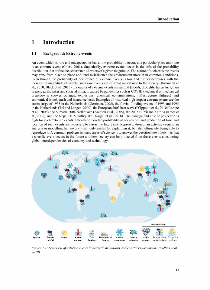
1 Introduction
1.1 ; (D’Ippoliti et al., 2010; Robine
Chapter 1
12
;. It is often referred to as “the curse of few observations”. A practical example 1.2 framework 1.2.1 1.2.1.1 tremes speeds. The UE’s may have tangible and direct ethical, social, economic and environmental impacts,
Introduction
13
analyse the UE’s statistically, there are mainly two methods. The first method relies on fitting ;;;; EVT provides a robust means of statistical modeling of UE’s thus making it suitable to use for hydro;; ; ; ; ;;;;1.2.1.2 ; ; ;;;; ;;;;
Chapter 1
14
;; 1.2.2 ; ; ;1.2.2.1; ;; ;
Introduction
15
; ; ; ;1.2.2.2 Representatio cryosphere ; ;;; ; ;;
Chapter 1
16
;;;–;;;;;;;; ; ;; ; ; ; ; ; ; ;;;;;; ;
Introduction
17
;; ; ; ;;;; 1.2.2.3 ; meš, 1990) ;;;;
Chapter 1
18
;;;;1.2.2.4 Spatio;; ;;;; ;;1.2.2.5 ;;;;; ; 1.2.2.6; ;;;;;sometimes referred to as “model uncertainty”
Introduction
19
; ; ; ; ;;–1.2.2.7 Coupli models overall response of the system doesn’t provide key knowledge on how ; ;;;;;;;;;;;; ; ; ;;;;;
Chapter 1
20
;;1.3 events 1.3.1 Definition ; ; ;;;;;;2014; Dunn et al., 2020; Kokkonen et al., 2006; Kundzewicz et al., 2014; O’Gorman, 2015);;; ;;;;
Introduction
21
“(1) two or more extreme contributing events can be of similar (clustered multiple events) or different type(s).” ;’“a combination of multiple drivers and/or hazards that contributes to societal or environmental risk” 1.3.2
Chapter 1
22
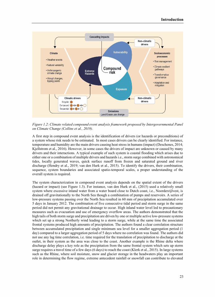
;;;;;;;;;;; ; ;;;; ; – ;;;; ; 1.3.3 ;;
Introduction
23
; ;
Chapter 1
24
; ; ; ;occurrence of flood in one river, or the other, or both hazard scenarios and both ‘OR’ and ‘AND’ hazard ; ;;e either ‘AND’ or ‘OR’, or both hazard scenarios are used. Multivariate hazard scenarios coula “Kendal”, “Survival Kendall” and “Structural” approach 1.3.4 ; ; ;
Introduction
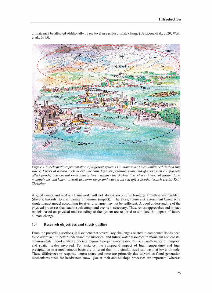
25
;
1.4 objectives outline
Chapter 1
26
RQ1RQ2
RQ3
RQ4 RQ1 3 RQ1 RQ2
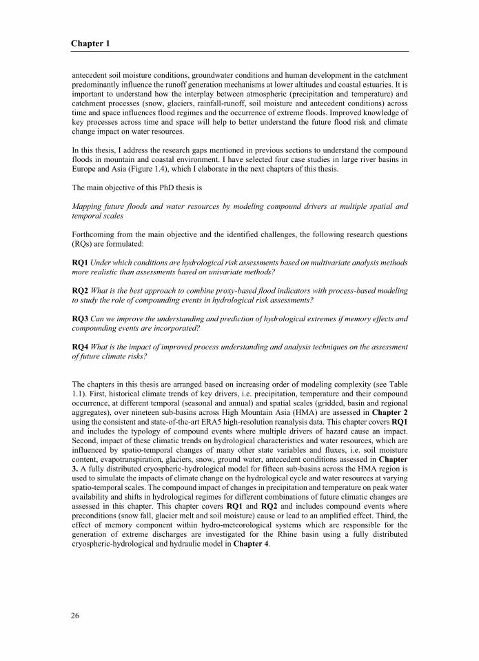
Introduction
27
Chapter 1
28
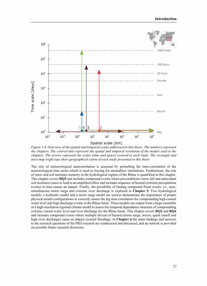
Chapterframe
Region Data Approach Impact

Introduction
29

2
Chapter 2Historical climate trends over High Mountain Asia derived from ERA5
reanalysis data

Chapter 2
32
Historical climate trends
33
2 Historical
; 2.1 ;; ;;;
Chapter 2
34
; ;;;; ;;;;; ;;;;;;;;;;;;;;;;;;; ; ; ; ;;;;;;;
Historical climate trends
35
;;;; ; ; 2.2 7−1132− 47 ; 2.3 – –
Chapter 2
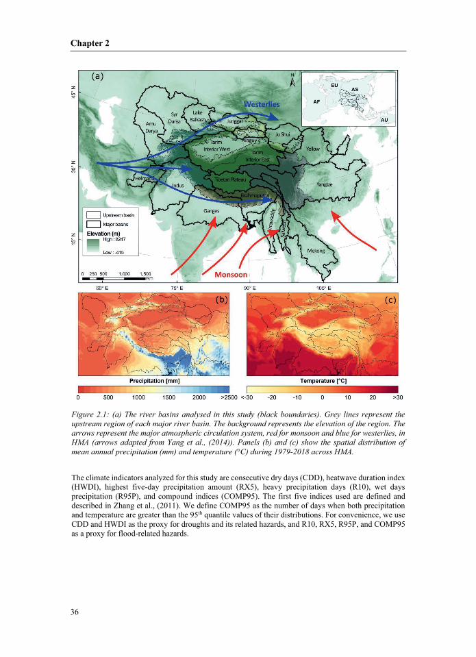
36
Historical climate trends
37
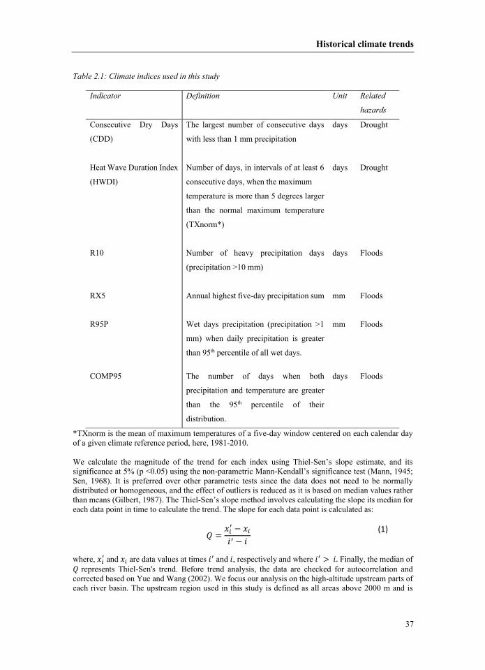
Sen’s slope estimate, and its ndall’s significance test ; Sen’s slope method involves calculating the slope its m 𝑄𝑄𝑄𝑄 = 𝑥𝑥𝑥𝑥𝑖𝑖𝑖𝑖
′ − 𝑥𝑥𝑥𝑥𝑖𝑖𝑖𝑖𝑖𝑖𝑖𝑖′ − 𝑖𝑖𝑖𝑖
(1)
𝑥𝑥𝑥𝑥𝑖𝑖𝑖𝑖
′𝑥𝑥𝑥𝑥𝑖𝑖𝑖𝑖𝑖𝑖𝑖𝑖′𝑖𝑖𝑖𝑖𝑖𝑖𝑖𝑖′ > 𝑖𝑖𝑖𝑖.𝑄𝑄𝑄𝑄
Chapter 2
38
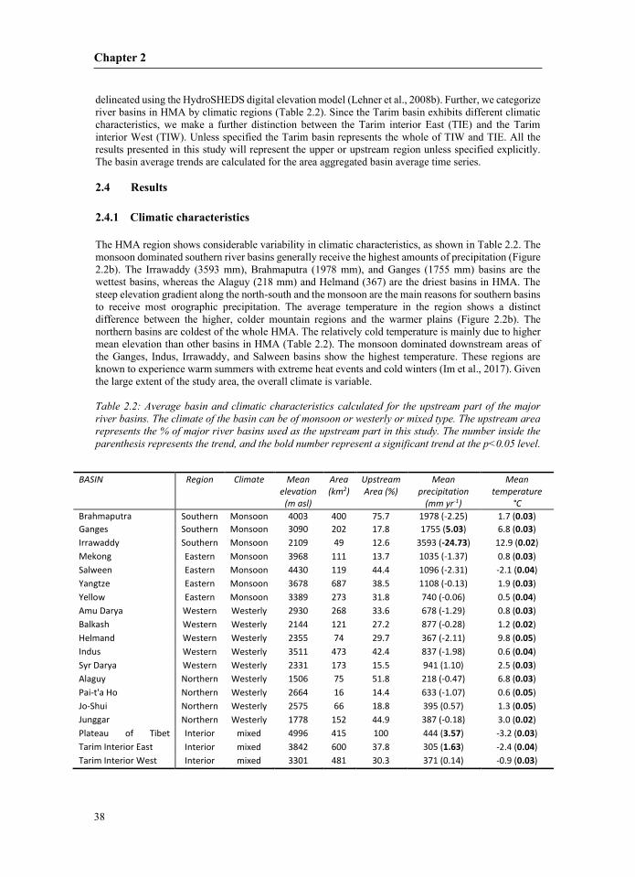
2.4 Results 2.4.1 characteristics
BASIN Region Climate Mean
elevation (m asl)
Area (km2)
Upstream Area (%)
Mean precipitation
(mm yr-1)
Mean temperature
°C Brahmaputra Southern Monsoon 4003 400 75.7 1978 (-2.25) 1.7 (0.03) Ganges Southern Monsoon 3090 202 17.8 1755 (5.03) 6.8 (0.03) Irrawaddy Southern Monsoon 2109 49 12.6 3593 (-24.73) 12.9 (0.02) Mekong Eastern Monsoon 3968 111 13.7 1035 (-1.37) 0.8 (0.03) Salween Eastern Monsoon 4430 119 44.4 1096 (-2.31) -2.1 (0.04) Yangtze Eastern Monsoon 3678 687 38.5 1108 (-0.13) 1.9 (0.03) Yellow
Eastern Monsoon 3389 273 31.8 740 (-0.06) 0.5 (0.04) Amu Darya Western Westerly 2930 268 33.6 678 (-1.29) 0.8 (0.03) Balkash Western Westerly 2144 121 27.2 877 (-0.28) 1.2 (0.02) Helmand Western Westerly 2355 74 29.7 367 (-2.11) 9.8 (0.05) Indus Western Westerly 3511 473 42.4 837 (-1.98) 0.6 (0.04) Syr Darya Western Westerly 2331 173 15.5 941 (1.10) 2.5 (0.03) Alaguy Northern Westerly 1506 75 51.8 218 (-0.47) 6.8 (0.03) Pai-t'a Ho Northern Westerly 2664 16 14.4 633 (-1.07) 0.6 (0.05) Jo-Shui Northern
Northern
rth
Westerly 2575 66 18.8 395 (0.57) 1.3 (0.05) Junggar Northern Westerly 1778 152 44.9 387 (-0.18) 3.0 (0.02) Plateau of Tibet Interior
Interior mixed 4996 415 100 444 (3.57) -3.2 (0.03) Tarim Interior East Interior mixed 3842 600 37.8 305 (1.63) -2.4 (0.04) Tarim Interior West Interior mixed 3301 481 30.3 371 (0.14) -0.9 (0.03)
Historical climate trends
39
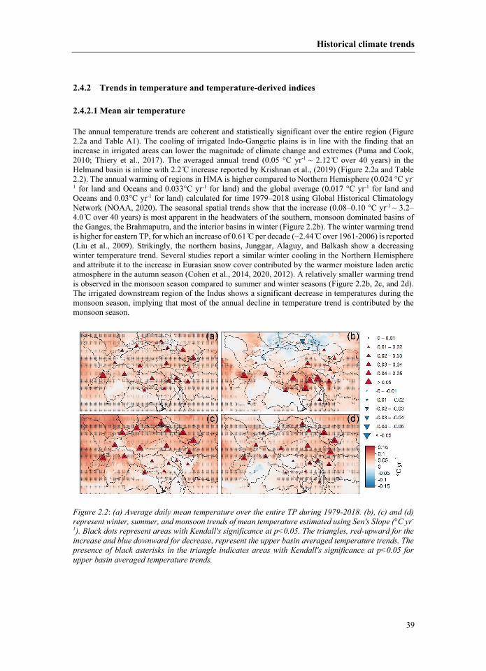
2.4.2 2.4.2.1 ; –––
Chapter 2
40
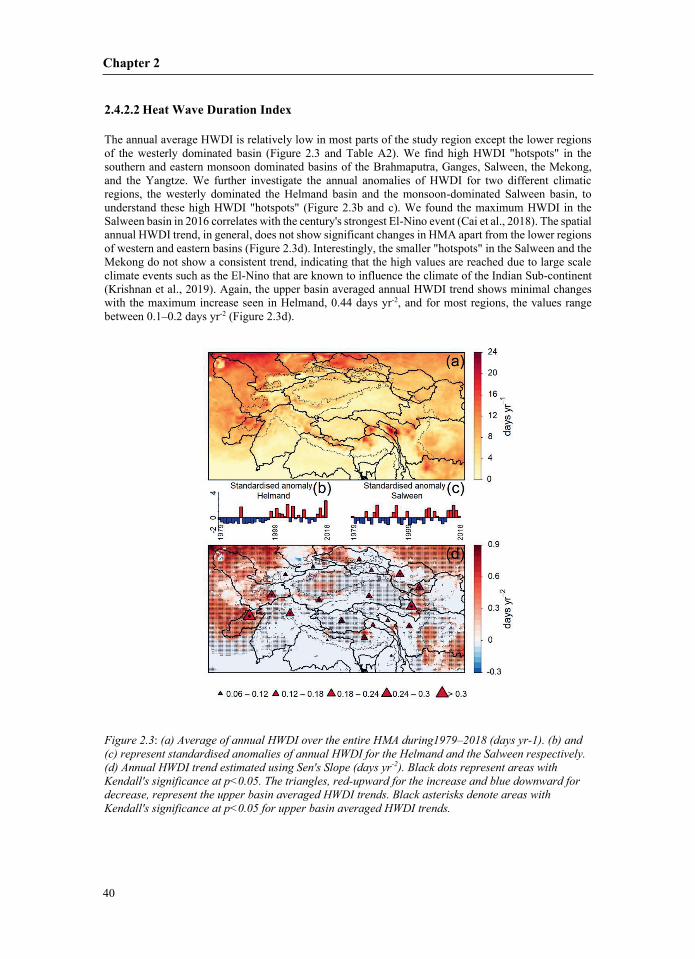
2.4.2.2 –
–
Historical climate trends
41
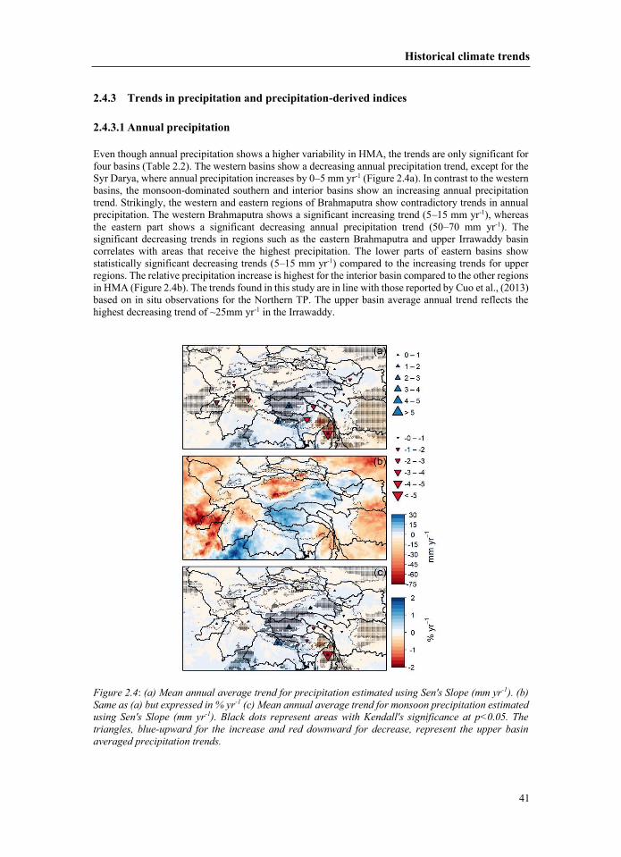
2.4.3 2.4.3.1 – – – –
Chapter 2
42
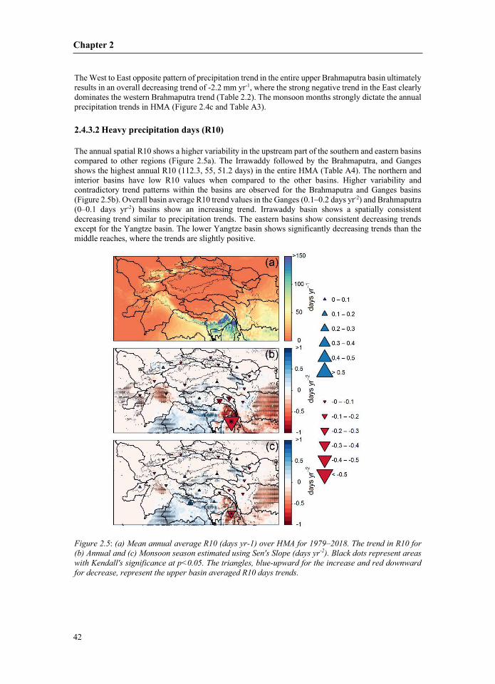
2.4.3.2 ––
–
Historical climate trends
43
2.4.3.3;
Chapter 2
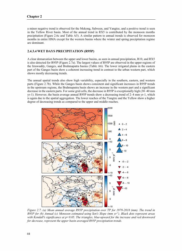
44
2.4.3.4 ( ––
Historical climate trends
45
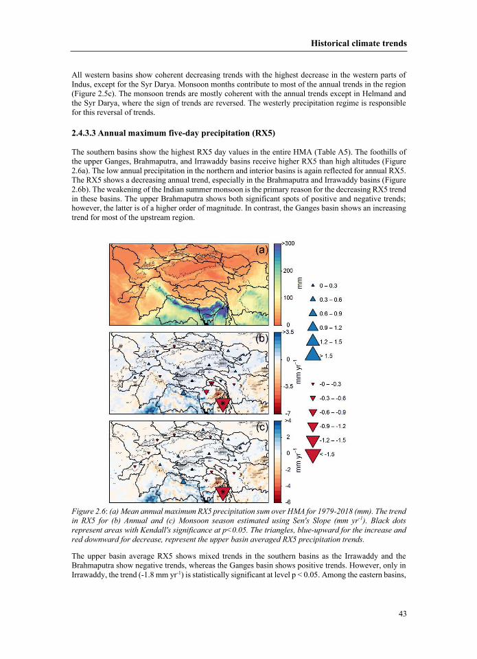
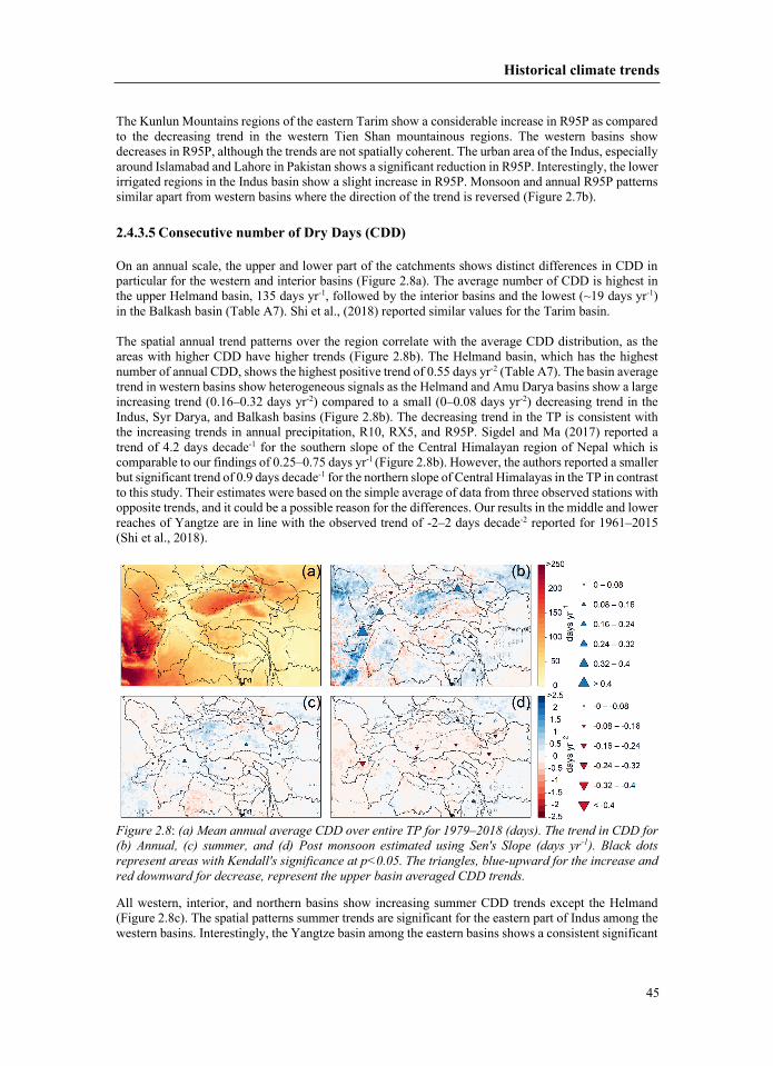
2.4.3.5 y –––––
–
Chapter 2
46
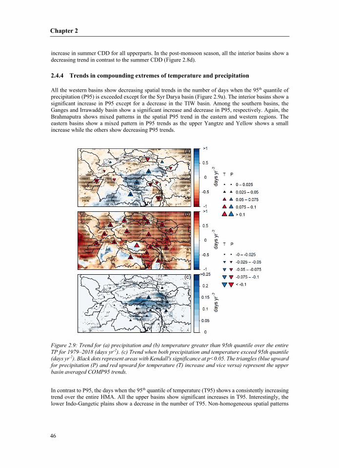
2.4.4
–
Historical climate trends
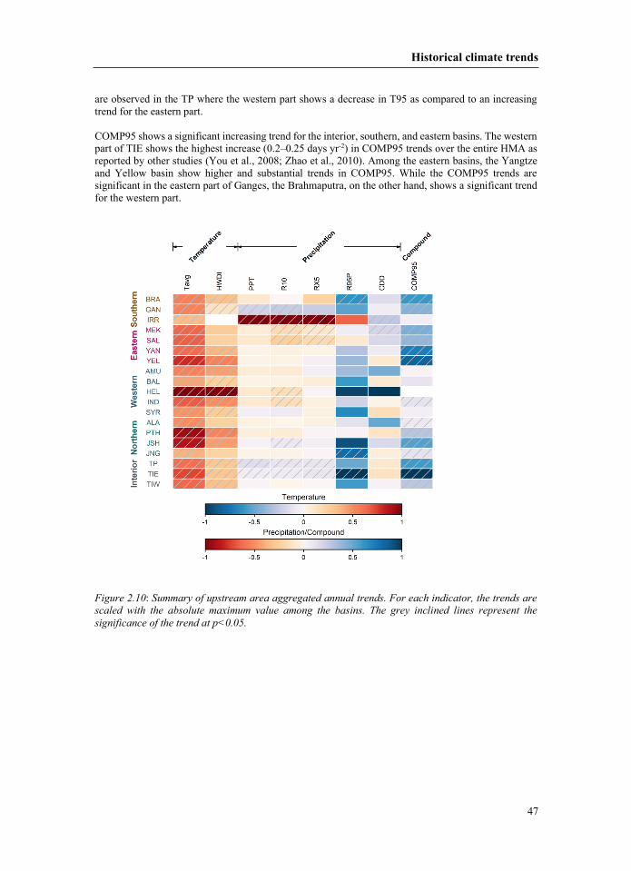
47
–;
Chapter 2
48
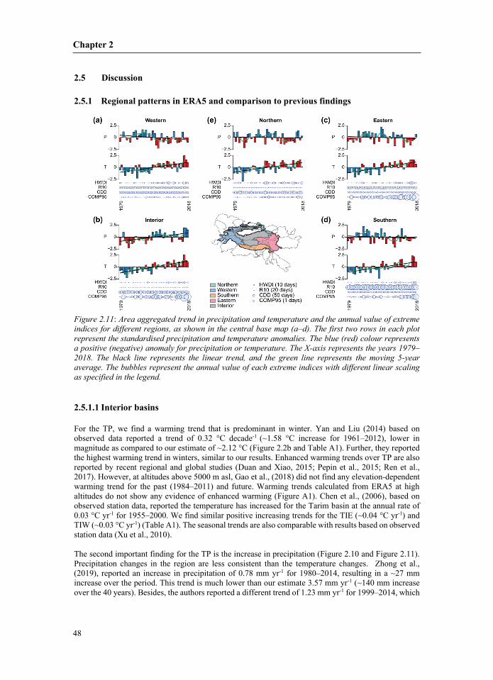
2.5 Discussion 2.5.1
––
2.5.1.1 – ;; – – – –
Historical climate trends
49
; ;; ;2.5.1.2 –;– – – –– –2.5.1.3 ;
Chapter 2
50
;; ;;;;;;;
2.5.1.4 East –; – ; 2.5.1.5 –––
;
Historical climate trends
51
2.5.2 2.5.2.1 ; ; ;;;;;; ;; ;;2.5.2.2 ;;;; ; ; ; ; ;;;;
Chapter 2
52
2.5.2.3 Heatwaves ;;;;; ;2.5.2.4 lows ; ;;;2.5.3 ;;;;;;;
Historical climate trends
53
;;2.6 Conclusions
Acknowledgments s also partly funded by the European Union’s and Innovation Program under the Marie Skłodowska

3
Chapter 3Variable 21st century climate change response for rivers in High Mountain
Asia at seasonal to decadal time scales

Chapter 3
56
Climate change response on hydrology
57
3 Variable
3.1 ; ; ; ;;;;;; ;;;; ;; ;;
Chapter 3
58
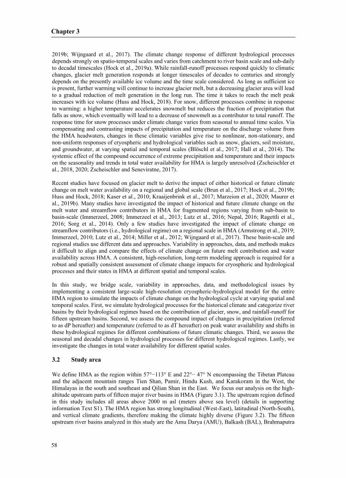
; ;;;;;;;; ;;;;; ;;;; 3.2 We define HMA as the region within 57°−113° E and 22°− 47° N encompassing the Tibetan Plateau
Climate change response on hydrology
59
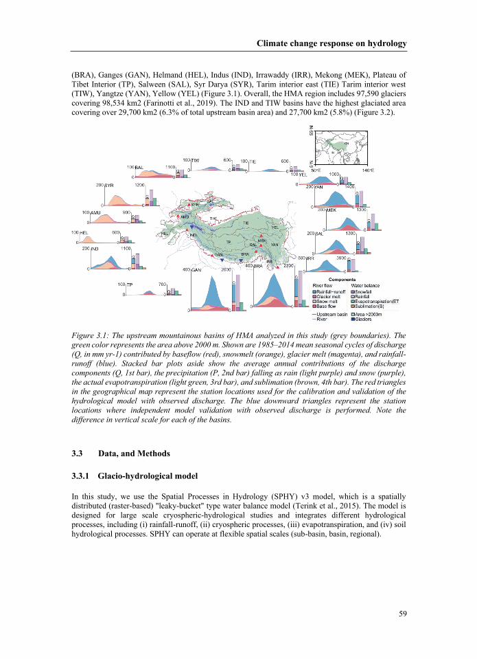
–
3.3 3.3.1
Chapter 3
60
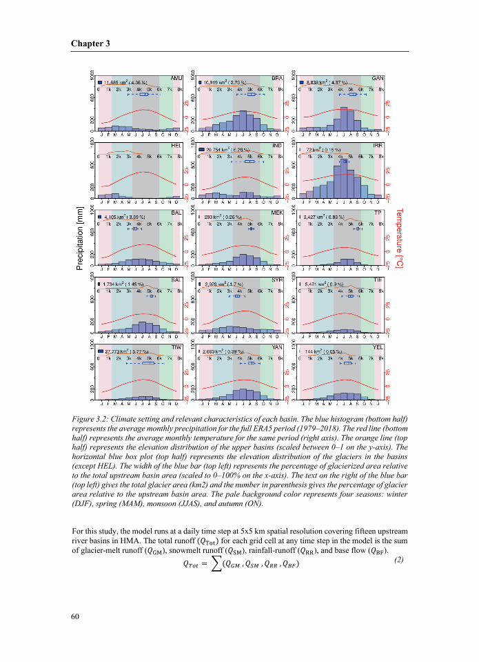
–– –
(𝑄𝑄𝑄𝑄Tot)𝑄𝑄𝑄𝑄GM𝑄𝑄𝑄𝑄SM𝑄𝑄𝑄𝑄RR𝑄𝑄𝑄𝑄BF
𝑄𝑄𝑄𝑄𝑇𝑇𝑇𝑇𝑇𝑇𝑇𝑇𝑇𝑇𝑇𝑇 = ∑(𝑄𝑄𝑄𝑄𝐺𝐺𝐺𝐺𝐺𝐺𝐺𝐺 , 𝑄𝑄𝑄𝑄𝑆𝑆𝑆𝑆𝐺𝐺𝐺𝐺 , 𝑄𝑄𝑄𝑄𝑅𝑅𝑅𝑅𝑅𝑅𝑅𝑅 , 𝑄𝑄𝑄𝑄𝐵𝐵𝐵𝐵𝐵𝐵𝐵𝐵)
Climate change response on hydrology
61
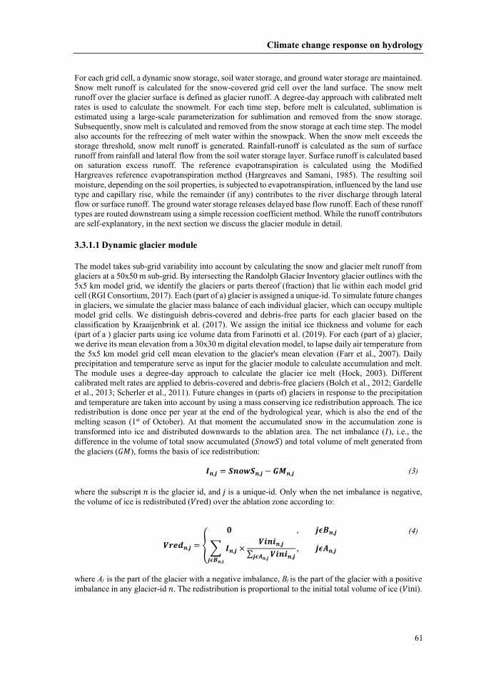
3.3.1.1 ;; 𝐼𝐼𝐼𝐼 (𝑆𝑆𝑆𝑆𝑆𝑆𝑆𝑆𝑆𝑆𝑆𝑆𝑆𝑆𝑆𝑆𝑆𝑆𝑆𝑆)𝐺𝐺𝐺𝐺𝐺𝐺𝐺𝐺
𝑰𝑰𝑰𝑰𝒏𝒏𝒏𝒏,𝒋𝒋𝒋𝒋 = 𝑺𝑺𝑺𝑺𝒏𝒏𝒏𝒏𝑺𝑺𝑺𝑺𝑺𝑺𝑺𝑺𝑺𝑺𝑺𝑺𝒏𝒏𝒏𝒏,𝒋𝒋𝒋𝒋 − 𝑮𝑮𝑮𝑮𝑮𝑮𝑮𝑮𝒏𝒏𝒏𝒏,𝒋𝒋𝒋𝒋
𝑆𝑆𝑆𝑆𝑗𝑗𝑗𝑗𝑉𝑉𝑉𝑉red
𝑽𝑽𝑽𝑽𝑽𝑽𝑽𝑽𝑽𝑽𝑽𝑽𝑽𝑽𝑽𝑽𝒏𝒏𝒏𝒏,𝒋𝒋𝒋𝒋 = 𝟎𝟎𝟎𝟎 , 𝒋𝒋𝒋𝒋𝒋𝒋𝒋𝒋𝑩𝑩𝑩𝑩𝒏𝒏𝒏𝒏,𝒋𝒋𝒋𝒋
∑ 𝑰𝑰𝑰𝑰𝒏𝒏𝒏𝒏,𝒋𝒋𝒋𝒋𝒋𝒋𝒋𝒋𝒋𝒋𝒋𝒋𝑩𝑩𝑩𝑩𝒏𝒏𝒏𝒏,𝒋𝒋𝒋𝒋
×𝑽𝑽𝑽𝑽𝑽𝑽𝑽𝑽𝒏𝒏𝒏𝒏𝑽𝑽𝑽𝑽𝒏𝒏𝒏𝒏,𝒋𝒋𝒋𝒋
∑ 𝑽𝑽𝑽𝑽𝑽𝑽𝑽𝑽𝒏𝒏𝒏𝒏𝑽𝑽𝑽𝑽𝒏𝒏𝒏𝒏,𝒋𝒋𝒋𝒋𝒋𝒋𝒋𝒋𝒋𝒋𝒋𝒋𝑨𝑨𝑨𝑨𝒏𝒏𝒏𝒏,𝒋𝒋𝒋𝒋, 𝒋𝒋𝒋𝒋𝒋𝒋𝒋𝒋𝑨𝑨𝑨𝑨𝒏𝒏𝒏𝒏,𝒋𝒋𝒋𝒋
𝑆𝑆𝑆𝑆𝑉𝑉𝑉𝑉ini
Chapter 3
62
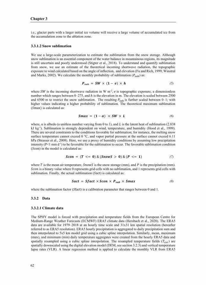
3.3.1.2 ;𝑃𝑃𝑃𝑃sub
𝑷𝑷𝑷𝑷𝒔𝒔𝒔𝒔𝒔𝒔𝒔𝒔𝒔𝒔𝒔𝒔 = 𝑺𝑺𝑺𝑺𝑺𝑺𝑺𝑺 × (𝟏𝟏𝟏𝟏 − 𝒆𝒆𝒆𝒆) × 𝒉𝒉𝒉𝒉 𝑆𝑆𝑆𝑆𝑆𝑆𝑆𝑆𝑒𝑒𝑒𝑒–ℎ 𝑃𝑃𝑃𝑃sub –; 𝑆𝑆𝑆𝑆max) 𝑺𝑺𝑺𝑺𝑺𝑺𝑺𝑺𝑺𝑺𝑺𝑺𝑺𝑺𝑺𝑺 = (𝟏𝟏𝟏𝟏 − 𝜶𝜶𝜶𝜶) × 𝑺𝑺𝑺𝑺𝑺𝑺𝑺𝑺 × 𝑳𝑳𝑳𝑳 where, α is albedo (a unitless number varying from 0 to 1), and 𝐿𝐿𝐿𝐿 ;𝑆𝑆𝑆𝑆con
𝑺𝑺𝑺𝑺𝑺𝑺𝑺𝑺𝑺𝑺𝑺𝑺𝑺𝑺𝑺𝑺 = (𝑻𝑻𝑻𝑻 <= 𝟎𝟎𝟎𝟎) & (𝑺𝑺𝑺𝑺𝑺𝑺𝑺𝑺𝑺𝑺𝑺𝑺𝑺𝑺𝑺𝑺𝑺𝑺𝑺𝑺 > 𝟎𝟎𝟎𝟎) & (𝑷𝑷𝑷𝑷 <= 𝟏𝟏𝟏𝟏) 𝑇𝑇𝑇𝑇𝑆𝑆𝑆𝑆𝑆𝑆𝑆𝑆𝑆𝑆𝑆𝑆𝑆𝑆𝑆𝑆𝑆𝑆𝑆𝑆𝑃𝑃𝑃𝑃𝑆𝑆𝑆𝑆𝑆𝑆𝑆𝑆𝑆𝑆𝑆𝑆𝑆𝑆𝑆𝑆𝑆𝑆𝑆𝑆act
𝑺𝑺𝑺𝑺𝑺𝑺𝑺𝑺𝑺𝑺𝑺𝑺𝑺𝑺𝑺𝑺 = 𝑺𝑺𝑺𝑺𝑺𝑺𝑺𝑺𝑺𝑺𝑺𝑺𝑺𝑺𝑺𝑺𝑺𝑺𝑺𝑺 × 𝑺𝑺𝑺𝑺𝑺𝑺𝑺𝑺𝑺𝑺𝑺𝑺𝑺𝑺𝑺𝑺 × 𝑷𝑷𝑷𝑷𝒔𝒔𝒔𝒔𝒔𝒔𝒔𝒔𝒔𝒔𝒔𝒔 × 𝑺𝑺𝑺𝑺𝑺𝑺𝑺𝑺𝑺𝑺𝑺𝑺𝑺𝑺𝑺𝑺 𝑆𝑆𝑆𝑆fact3.3.2 3.3.2.1 – 𝑇𝑇𝑇𝑇cor
Climate change response on hydrology
63
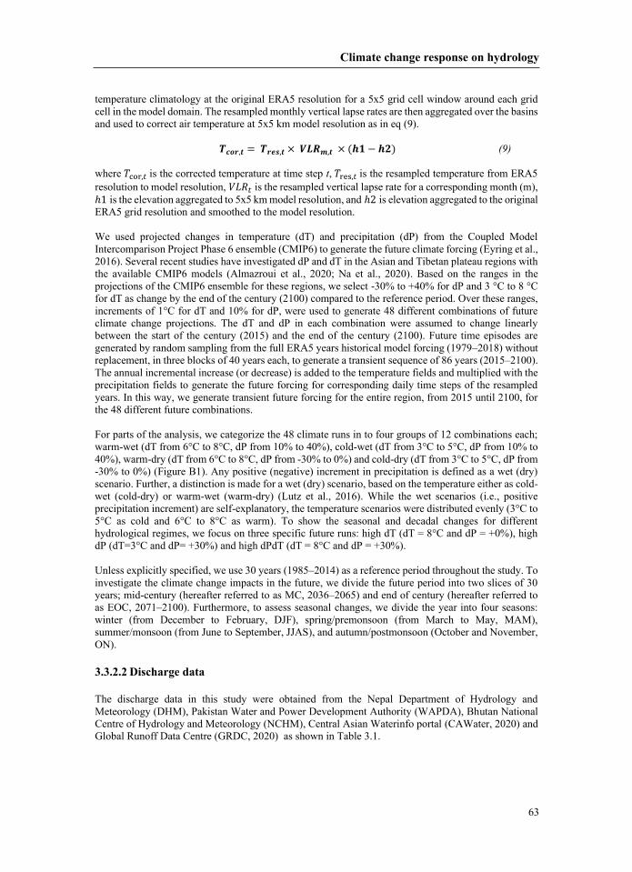
𝑻𝑻𝑻𝑻𝒄𝒄𝒄𝒄𝒄𝒄𝒄𝒄𝒄𝒄𝒄𝒄,𝒕𝒕𝒕𝒕 = 𝑻𝑻𝑻𝑻𝒄𝒄𝒄𝒄𝒓𝒓𝒓𝒓𝒓𝒓𝒓𝒓,𝒕𝒕𝒕𝒕 × 𝑽𝑽𝑽𝑽𝑽𝑽𝑽𝑽𝑽𝑽𝑽𝑽𝒎𝒎𝒎𝒎,𝒕𝒕𝒕𝒕 × (𝒉𝒉𝒉𝒉𝟏𝟏𝟏𝟏 − 𝒉𝒉𝒉𝒉𝟐𝟐𝟐𝟐)
𝑇𝑇𝑇𝑇cor,𝑡𝑡𝑡𝑡 𝑇𝑇𝑇𝑇res,𝑡𝑡𝑡𝑡 𝑉𝑉𝑉𝑉𝑉𝑉𝑉𝑉𝑉𝑉𝑉𝑉𝑡𝑡𝑡𝑡ℎ1ℎ2 ; ––; –;–– 3.3.2.2
Chapter 3
64
3.3.2.3 – 3.3.3 3.3.3.1 ;;;
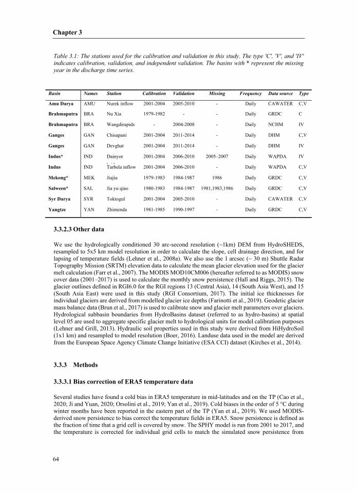
Basin Names Station
period
Validation
period
Missing
Years
Frequency Type
–
Climate change response on hydrology
65
; 𝑇𝑇𝑇𝑇crit DDFs3.3.3.2
𝑆𝑆𝑆𝑆fact𝑆𝑆𝑆𝑆fact
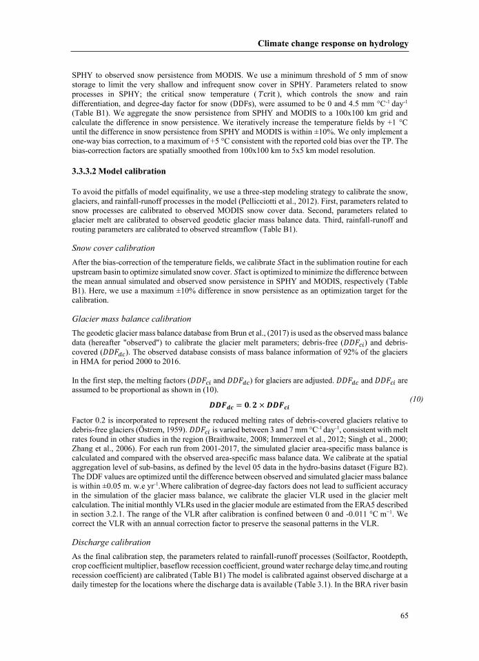
; 𝐷𝐷𝐷𝐷𝐷𝐷𝐷𝐷𝐷𝐷𝐷𝐷𝑐𝑐𝑐𝑐𝑐𝑐𝑐𝑐 𝐷𝐷𝐷𝐷𝐷𝐷𝐷𝐷𝐷𝐷𝐷𝐷𝑑𝑑𝑑𝑑𝑐𝑐𝑐𝑐𝐷𝐷𝐷𝐷𝐷𝐷𝐷𝐷𝐷𝐷𝐷𝐷𝑐𝑐𝑐𝑐𝑐𝑐𝑐𝑐𝐷𝐷𝐷𝐷𝐷𝐷𝐷𝐷𝐷𝐷𝐷𝐷𝑑𝑑𝑑𝑑𝑐𝑐𝑐𝑐𝐷𝐷𝐷𝐷𝐷𝐷𝐷𝐷𝐷𝐷𝐷𝐷𝑑𝑑𝑑𝑑𝑐𝑐𝑐𝑐𝐷𝐷𝐷𝐷𝐷𝐷𝐷𝐷𝐷𝐷𝐷𝐷𝑐𝑐𝑐𝑐𝑐𝑐𝑐𝑐
𝑫𝑫𝑫𝑫𝑫𝑫𝑫𝑫𝑫𝑫𝑫𝑫𝒅𝒅𝒅𝒅𝒅𝒅𝒅𝒅 = 𝟎𝟎𝟎𝟎. 𝟐𝟐𝟐𝟐 × 𝑫𝑫𝑫𝑫𝑫𝑫𝑫𝑫𝑫𝑫𝑫𝑫𝒅𝒅𝒅𝒅𝒄𝒄𝒄𝒄
𝐷𝐷𝐷𝐷𝐷𝐷𝐷𝐷𝐷𝐷𝐷𝐷𝑐𝑐𝑐𝑐𝑐𝑐𝑐𝑐;;; −
Chapter 3
66
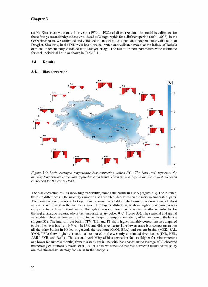
;– 3.4 Results 3.4.1
Climate change response on hydrology
67
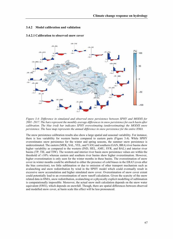
3.4.2 3.4.2.1
–
Chapter 3
68
3.4.2.2
3.4.2.3 ;
1) 1)AMU BRA
IRR BAL MEK TP SAL SYR TIE TIW
Climate change response on hydrology
69
– ; ;; 3.4.3
Chapter 3
70
;
Climate change response on hydrology
71
;;;; : –
Precipitation Area Glacier Runoff Runoff coef.
CV of runoff Glacier Snow Rainfall Base
Melt
Basin (mm yr-1) (Km2) area (%) (mm yr-1) - (%) melt melt runoff flow (%)
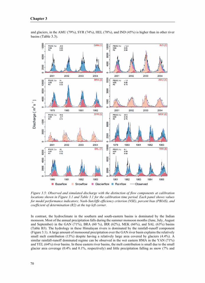
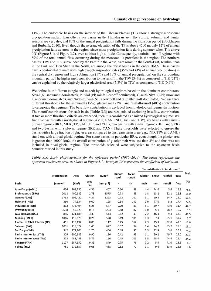
Amu Darya (AMU) 676 268,280 4.36 407 0.60 89 4.4 74.4 5.4 15.8 78.8 Brahmaputra (BRA) 2018 400,182 2.73 1575 0.78 85 1.8 13.2 62.1 22.8 15.0 Ganges (GAN) 1763 202,420 4.37 1293 0.73 101 3.1 10.3 64.7 22.0 13.4 Helmand (HEL) 360 74,334 0.00 195 0.54 140 0.0 77.5 5.2 17.4 77.5 Indus Basin (IND) 832 473,494 6.28 577 0.70 83 5.1 39.7 43.9 11.4 44.7 Irrawaddy (IRR) 3638 49,029 0.15 3223 0.88 87 0.0 5.1 78.2 16.7 5.1 Lake Balkash (BAL) 856 121,185 3.39 543 0.62 43 2.2 46.3 9.3 42.3 48.5 Mekong (MEK) 1066 110,678 0.26 528 0.49 101 0.3 7.4 55.1 37.2 7.7 Plateau of Tibet Interior (TP) 451 415,197 0.83 117 0.25 162 2.3 15.3 32.8 49.6 17.6 Salween (SAL) 1091 119,377 1.45 627 0.57 94 1.4 14.7 55.7 28.3 16.1 Syr Darya (SYR) 942 172,704 1.70 456 0.48 97 1.3 72.9 5.6 20.2 74.2 Tarim Interior East (TIE) 305 600,182 0.90 126 0.42 93 1.1 20.2 49.7 29.0 21.3 Tarim Interior West (TIW) 373 481,481 5.77 166 0.45 103 5.8 28.4 44.4 21.4 34.2 Yangtze (YAN) 1127 687,150 0.39 849 0.75 76 0.2 5.5 71.0 23.3 5.7 Yellow (YEL) 751 272,857 0.05 468 0.62 77 0.1 9.6 63.9 26.5 9.6
Chapter 3
72
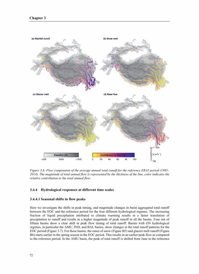
–
3.4.4 3.4.4.1
Climate change response on hydrology
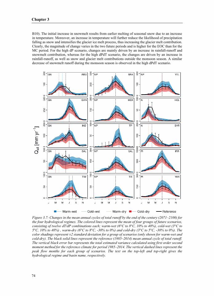
73
Chapter 3
74
–;––
Climate change response on hydrology
75
–
WARM WET COLD WET WARM DRY COLD DRYAMU GAN IND BAL TIW BRA MEK TP SAL TIE YEL HEL SYR IRR YAN
3.4.4.2
Chapter 3
76
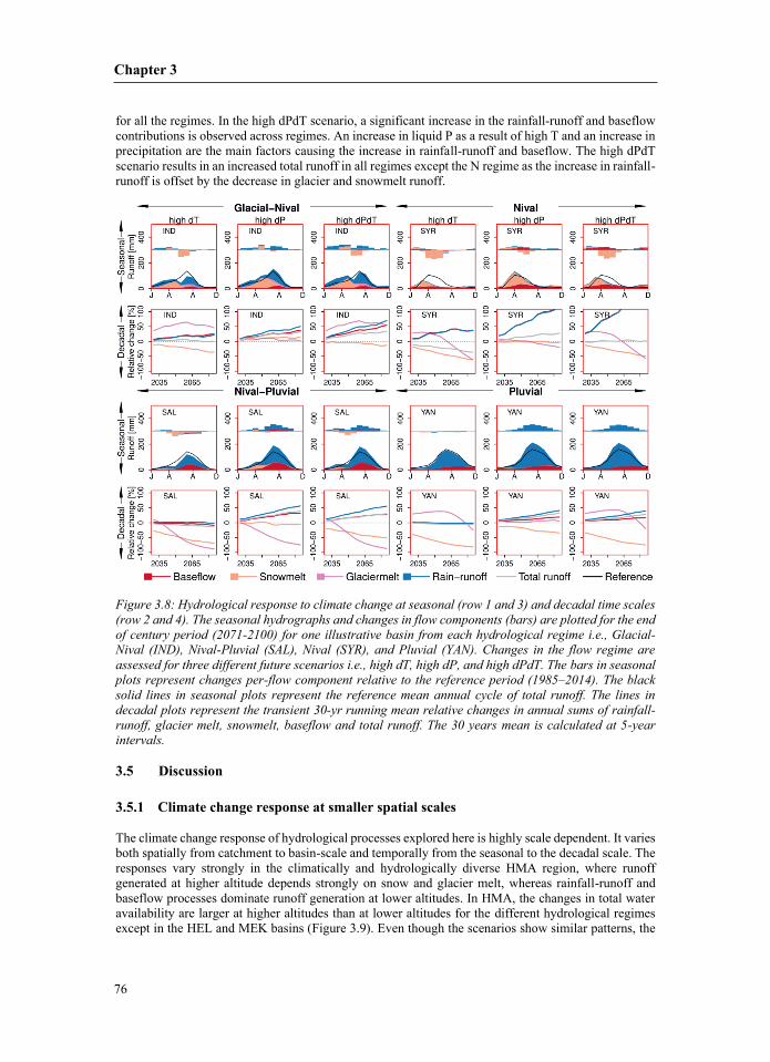
– 3.5 Discussion 3.5.1
Climate change response on hydrology
77
; 3.5.2 3.5.3 ;;––––;
Chapter 3
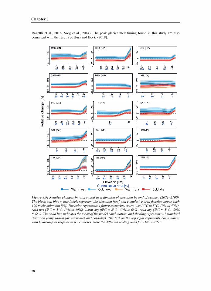
78
;
: –;
Climate change response on hydrology
79
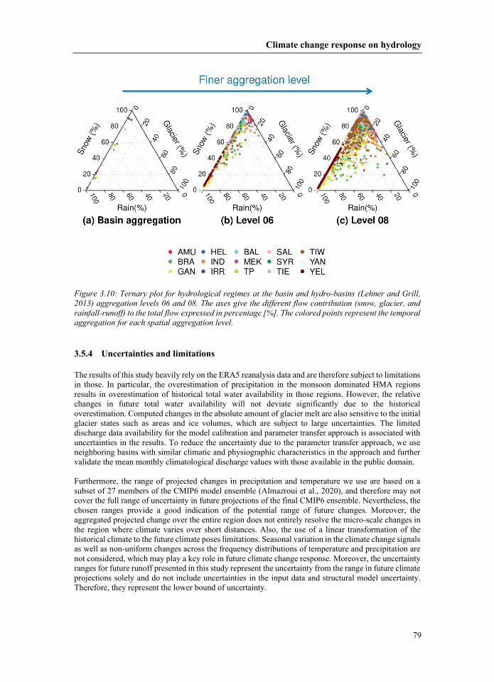
3.5.4 Uncer
Chapter 3
80
3.6 Conclusions
Acknowledgments Horizon 2020 Research and Innovation Program under the Marie Skłodowska‐Curie grant RC) under the European Union’s Horizon 2020

Climate change response on hydrology
81

4
Chapter 4The Impact of Meteorological and
Hydrological Memory on Compound Peak Flows in the Rhine River Basin

Chapter 4
84
Impact of memory on peak flows
85
4
– ; ; ; ; ; 4.1 ;;; ;longer time scales “remember” past atmospheric anomalies and their effects are reflected in subsequent ; ; ;;; —or ‘Hurst phenomenon’— ; ; ; ;;;;
Chapter 4
86
; ; ; ; ; ; ; ; ;;; ; ;;;;; ;per analysis for such CE’s requires a consistent long spatialtask to analyze the CE’s f ;; ;;
Impact of memory on peak flows
87
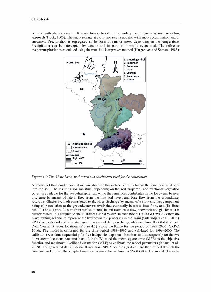
4.2 rea ;; “design discharge” of 16,000 4.3 4.3.1 Data–were adjusted to local topography using a vertical lapse rate of −6.4.3.2 based) “leakybucket” type model. The model –;
Chapter 4
88
– – –
Impact of memory on peak flows
89
referred to as ‘routing model’). Therouting model is calibrated for the Manning’s n value using the 4.3.3 4.3.4 4.3.5 ;
Chapter 4
90
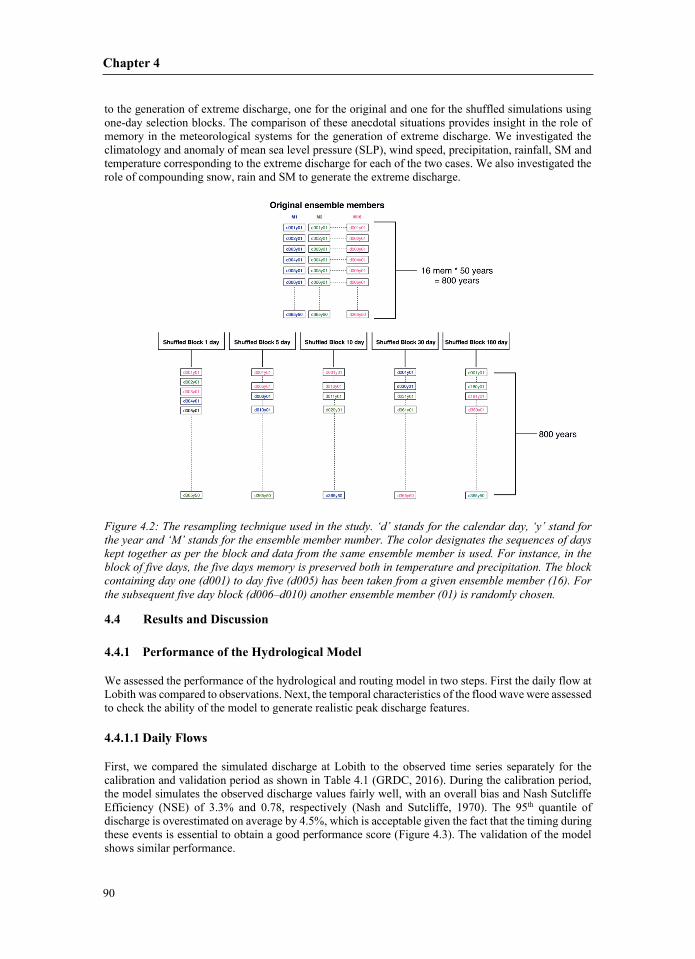
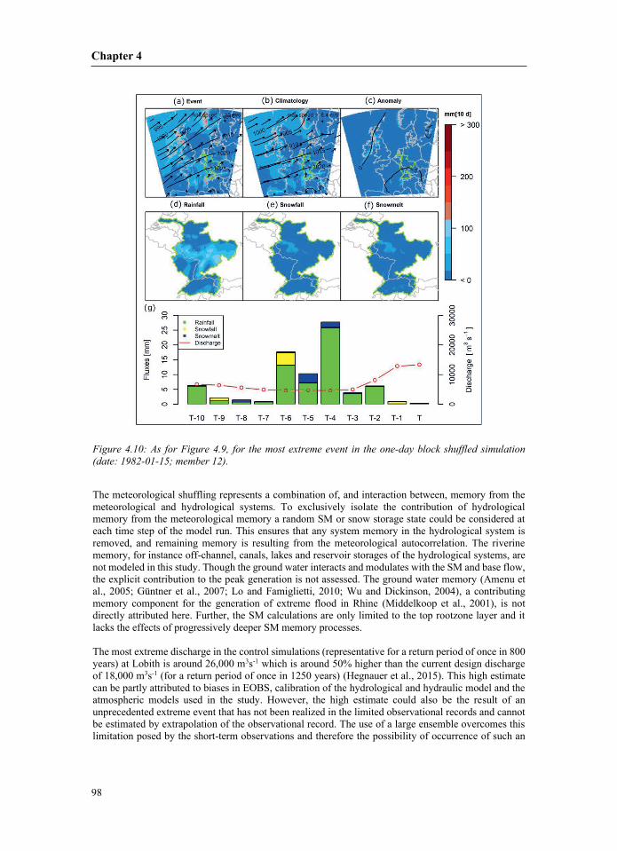
The resampling technique used in the study. ‘d’ stands for the calendar day, ‘y’ stand for the year and ‘M’ stands for the ensemble member number. The color designates the sequenc–
4.4 4.4.1 4.4.1.1
Impact of memory on peak flows
91
––
Calibration Validation
–
3 1 R2
–
4.4.1.2 –
Chapter 4
92
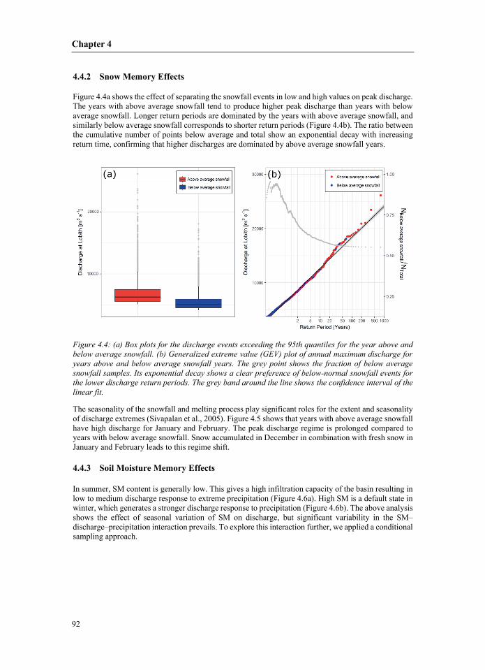
4.4.2
4.4.3 ––
Impact of memory on peak flows
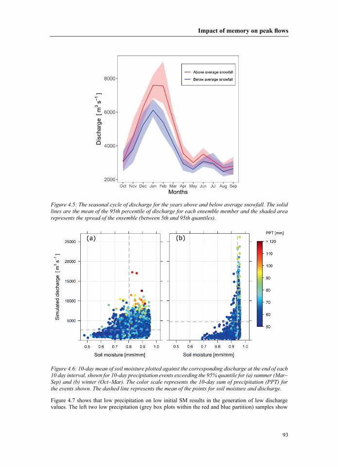
93
––
Chapter 4
94
; ;;
4.4.4 Autocorrelation 4.4.4.1 ;
Impact of memory on peak flows
95
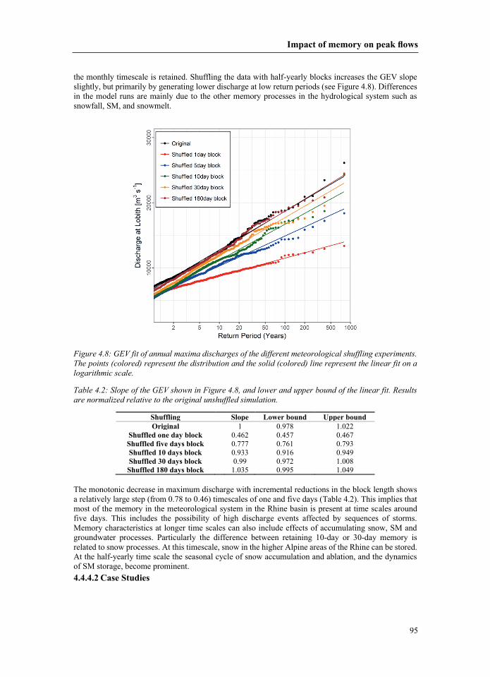
Shuffling Slope undOriginal
4.4.4.2 C
Chapter 4
96
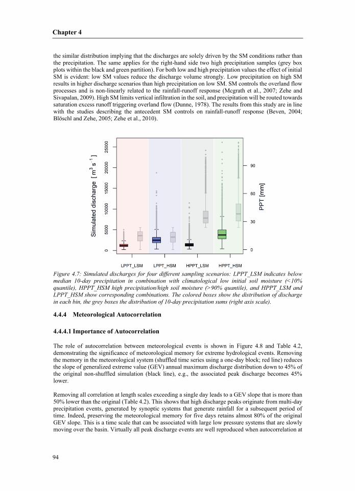
;;;
;–
Impact of memory on peak flows
97
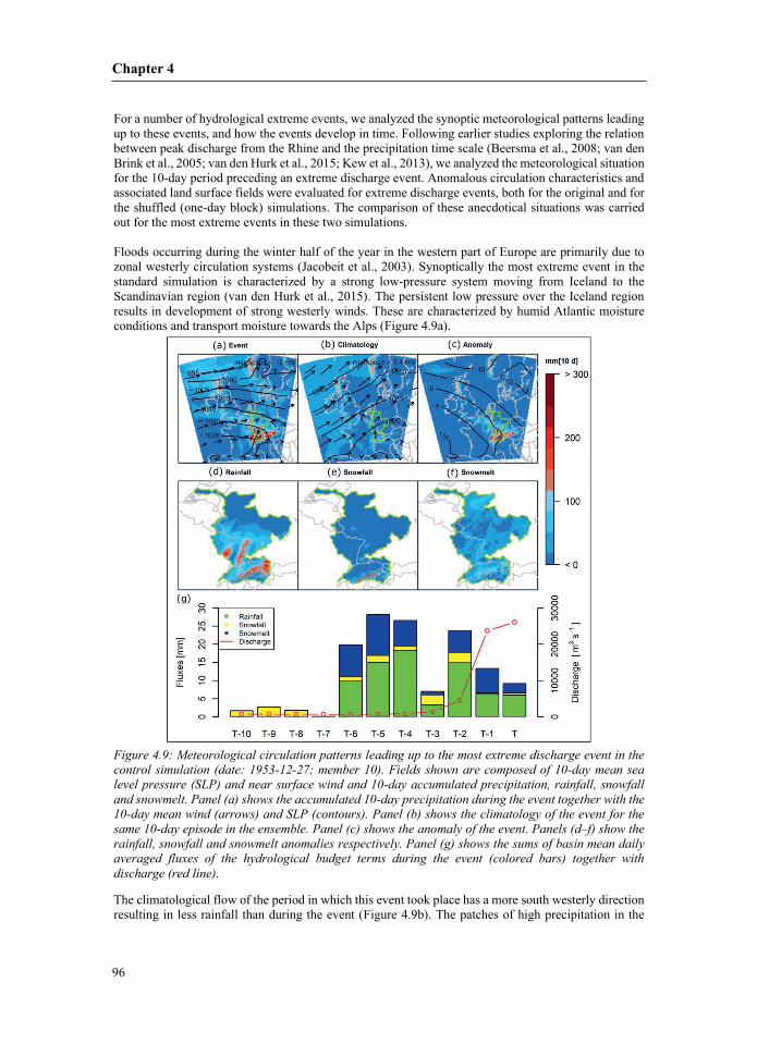
;; consistent with the evolution of the region’s temperature ( 4.5 ;; ; ; ;;;
Chapter 4
98
;
; ; ;
Impact of memory on peak flows
99
;;;;;;; ; ; ; ; ;—;—
was funded by the European Union’sion’s Horizon

5
Chapter 5Storm surge and extreme river discharge:
a compound event analysis using ensemble impact modelling

Chapter 5
102
Strom surge and extreme river discharge
103
5
5.1 ; ; ; ;;
Chapter 5
104
;;;;; – ; –
Strom surge and extreme river discharge
105
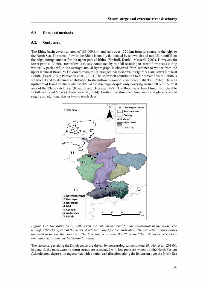
5.2 Data 5.2.1 ; ;
Chapter 5
106
5.2.2 ; – 5.2.3 e 96 uted, physically based “leakybucket” type model, which operates on a gridpoint basis. It integrates parameterizations of the dominant –; ;
Strom surge and extreme river discharge
107
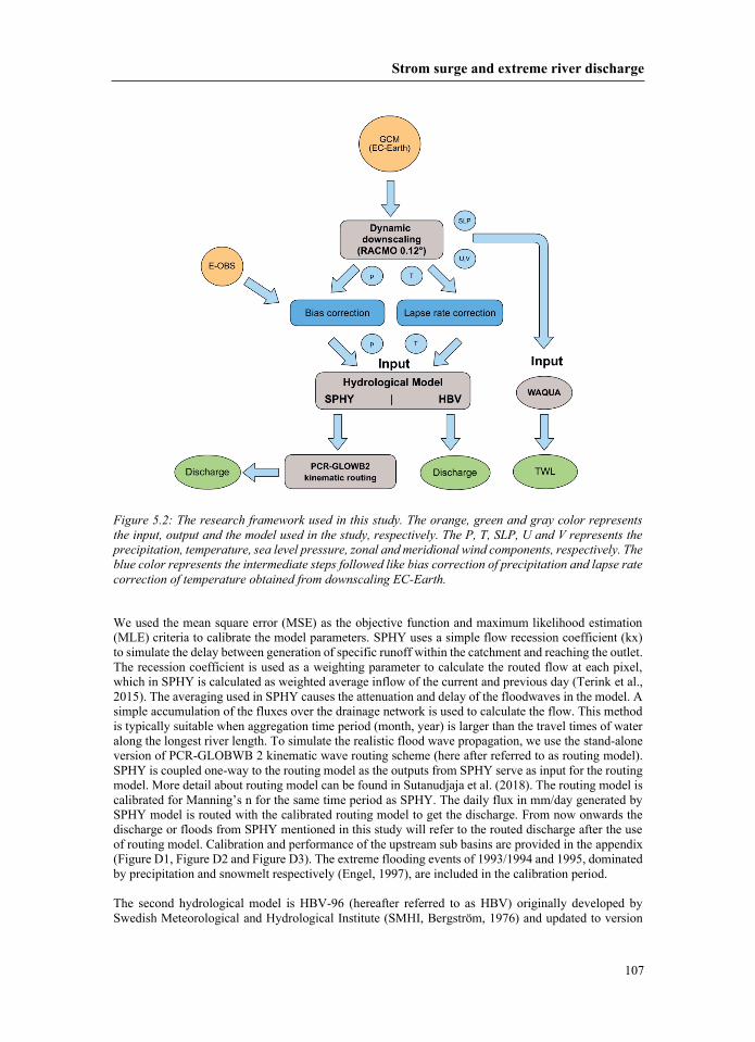
calibrated for Manning’s n for the same time period as SPHY. The daily flux in mm/day generated by
Chapter 5
108
. HBV is a “semied” conceptual model and, similar to 5.2.4 5.3 ; 5.3.1 –
Strom surge and extreme river discharge
109
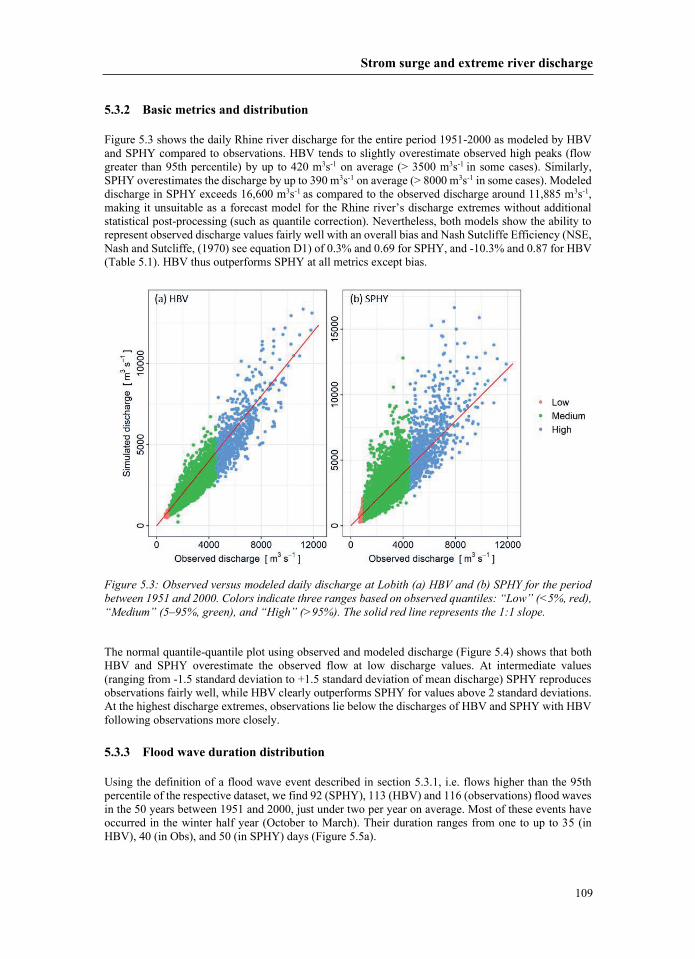
5.3.2 and a forecast model for the Rhine river’s discharge extremes without additional
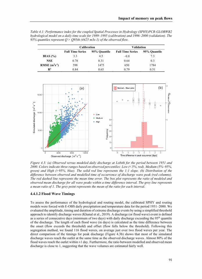
antiles: “Low” “Medium” (5–95%, green), and “High” (>95%). The solid red line represents the 1:1 slope.
5.3.3
Chapter 5
110
HBV SPHY
Med High All Med High All
R2
3s 1
NSE
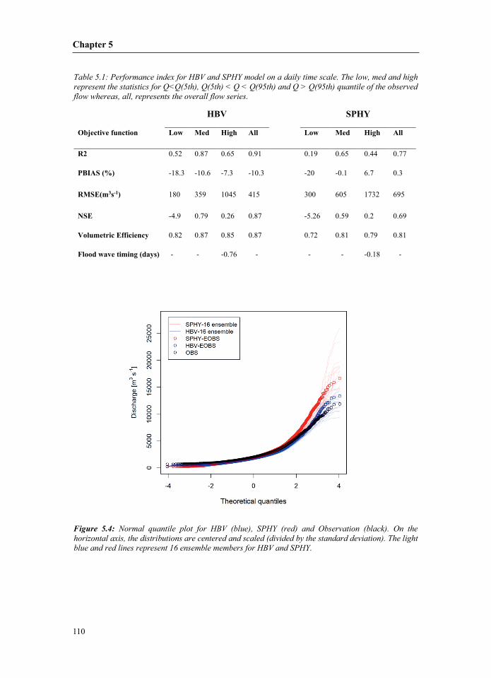
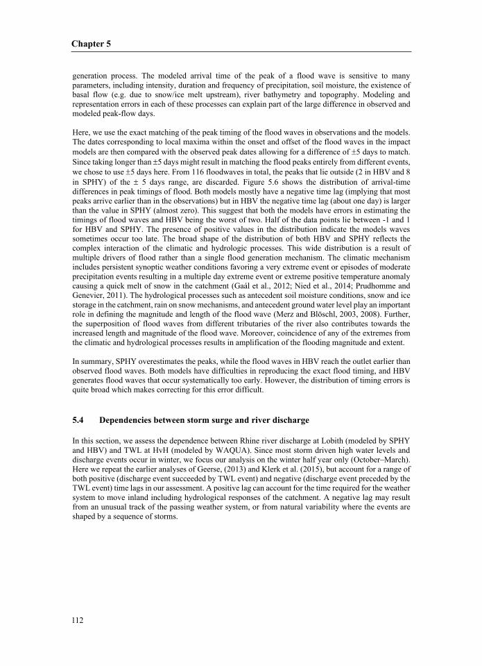
5.4:
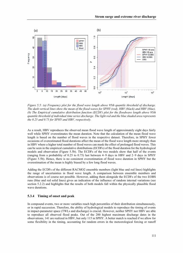
Strom surge and extreme river discharge
111
– – 5.3.4
(a) (b)
Chapter 5
112
;; 5.4 Depende –
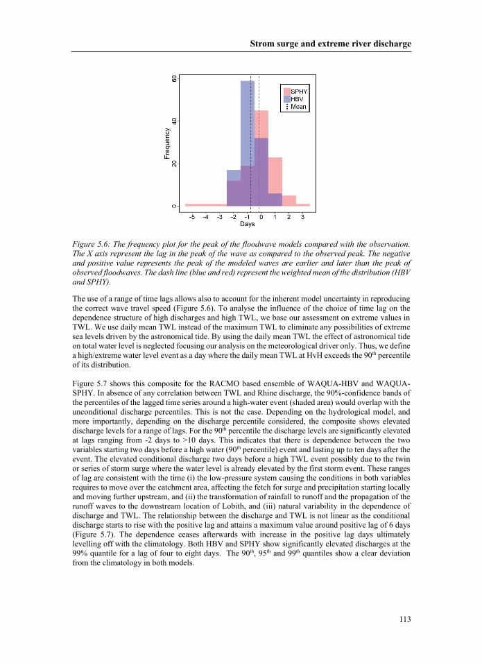
Strom surge and extreme river discharge
113
Chapter 5
114
;
5.4.1
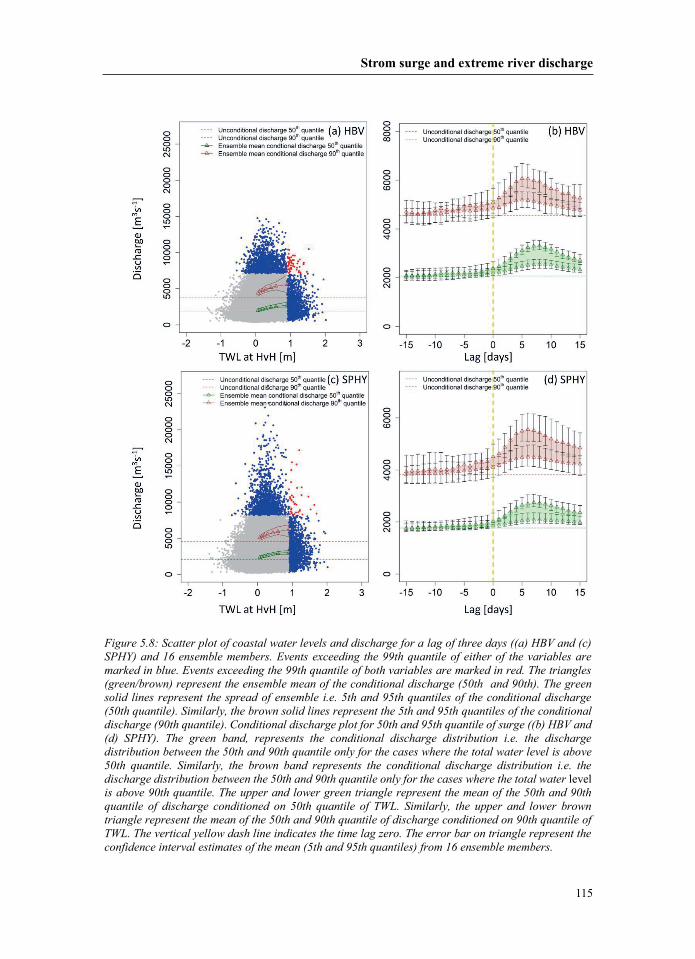
Strom surge and extreme river discharge
115
Chapter 5
116
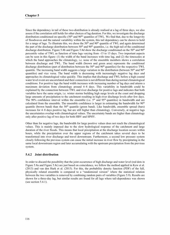
– – 5.4.2 physically related ensemble is compared to a “randomized version” where the statistical relation
Strom surge and extreme river discharge
117
correspond to the highest TWL (∆), discharge (+) and compound events (o) for individual ensemble
Chapter 5
118
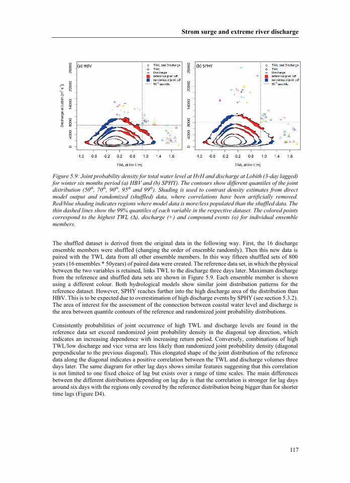
5.4.3 as “random chance” as these are not dep ––
5.5
Strom surge and extreme river discharge
119
k succession (“twin storms”) where the second storm coincides wis explained by “twin storms” ; ;
Chapter 5
120
5.6
Strom surge and extreme river discharge
121
Com
funding from the European Union’s Horizon 2020 research and inprogramme under the Marie Skłodowskaect “Impacted by Coincident Weather Extremes” (ICOWEX; grand n

6

Chapter 6Synthesis

Chapter 6
124
Conclusion
125
6 Synthesis
; ; Table 1.1 6.1 which
realistic than ar ;;;
Chapter 6
126
6.2
?
; ;
Conclusion
127
6.3
? ; ;; ; ;
Chapter 6
128
6.4?
;;;. Inclusion of sublimation process in the simulation of HMA’s hydrology significantly ;; ;; SPHY is coupled with a kinematic wave routing scheme and calibrated based on the Manning’s n
6.5
•
Conclusion
129
•
•
•
6.6 Recommendations 6.6.1
6.6.1.1 ;
Chapter 6
130
;;;;; ;;; ;;;;; ; ;;
Conclusion
131
;; ; ; ; ; ; ; ;; ;; ;6.6.1.2
Chapter 6
132
libration parameter i.e., ‘kx’) implemented within the PCRaster modelling ;; . The method uses calibration of Manning’s n ;; 6.6.2
; ; ; ;;;;; ;;;; ;;; ; ; ;;;; ;
Conclusion
133
;;;6.6.3 ;;;; ;;;;;; ;; ;; ; 6.6.4 C s‘topdown approach’ to a ‘bottomup approach’. The traditional top
Chapter 6
134
; ; ;;; ; ; ; resolution (< 4 ;

135
Appendix

136
Appendix A
137
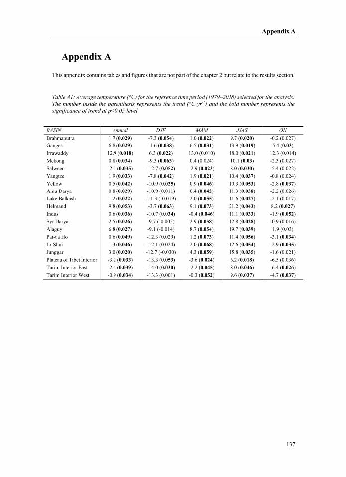
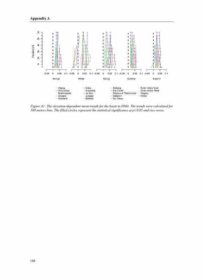
Appendix A
–
0.029 0.054 0.022 0.020 0.029 0.038 0.031 0.019 0.03 0.018 0.022 0.021 0.034 0.063 0.03 0.035 0.052 0.023 0.030 0.033 0.042 0.021 0.037 0.042 0.025 0.046 0.053 0.037 0.029 0.042 0.038 0.022 0.055 0.027 0.053 0.063 0.073 0.043 0.027 0.036 0.034 0.046 0.033 0.052 0.026 0.058 0.028 0.027 0.054 0.039 0.049 0.073 0.056 0.034 0.046 0.068 0.054 0.035 0.020 0.059 0.035 0.033 0.053) 0.024 0.018 0.039 0.030 0.045 0.046 0.026 0.034 0.052 0.037 0.037
Appendix A
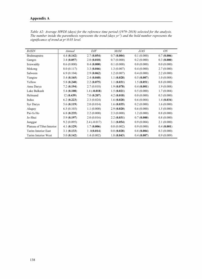
138
–
0.142 0.054 0.004 0.006 0.057 0.018 0.000 0.000 0.046 0.062 0.165 0.048 0.028 0.007 0.240 0.075 0.031 0.051 0.194 0.078 0.001 0.108 0.018 0.021 0.439 0.207 0.018 0.223 0.028 0.034 0.119 0.035 0.020 0.235 0.197 0.031 0.000 0.054 0.129 0.006 0.001 0.133 0.014 0.028 0.004 0.142 0.043 0.007
Appendix A
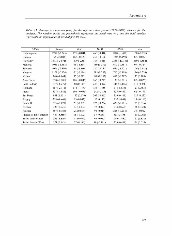
139
–
0.891 5.018 5.495 24.725 2.85 13.746 3.858 0.334 0.610 2.13 3.565 3.196 1.625 1.447 0.121
Appendix A
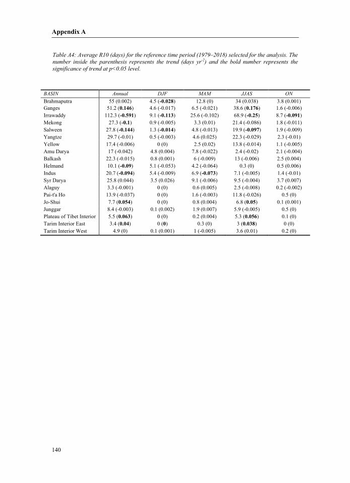
140
–
0.028 0.146 0.176 0.591 0.113 0.25 0.091 0.1 0.144 0.014 0.097 0.09 0.094 0.073 0.054 0.05 0.063 0.056 0.04 0 0.038
Appendix A
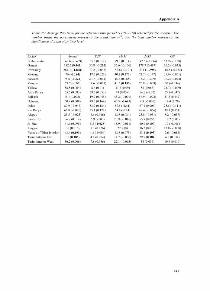
141
–
1.808 1.595 0.184 ( 0.322 0.153 0.645 0.26 0.44 0.028 0.193 0.193 0.186 0.184
Appendix A
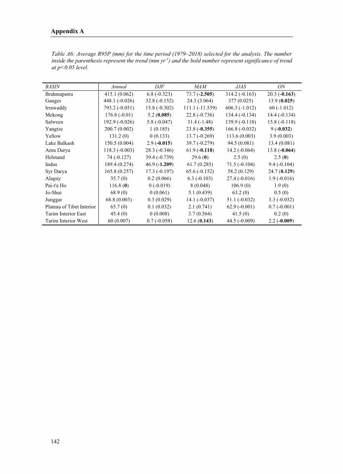
142
–
2.505 0.163 0.025 0.085 0.355 0.032 0.015 0.118 0.064 0 0 1.209 0.129 0 0.143 0.009
Appendix A
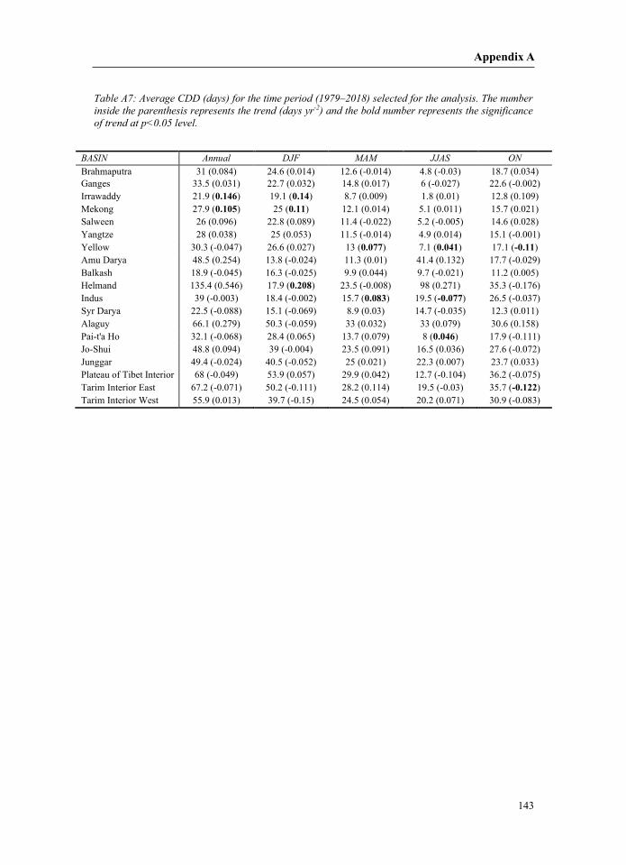
143
–
0.146 0.14 0.105 0.11 0.077 0.041 0.11 0.208 0.083 0.077 0.046 0.122
Appendix A
144
Appendix B
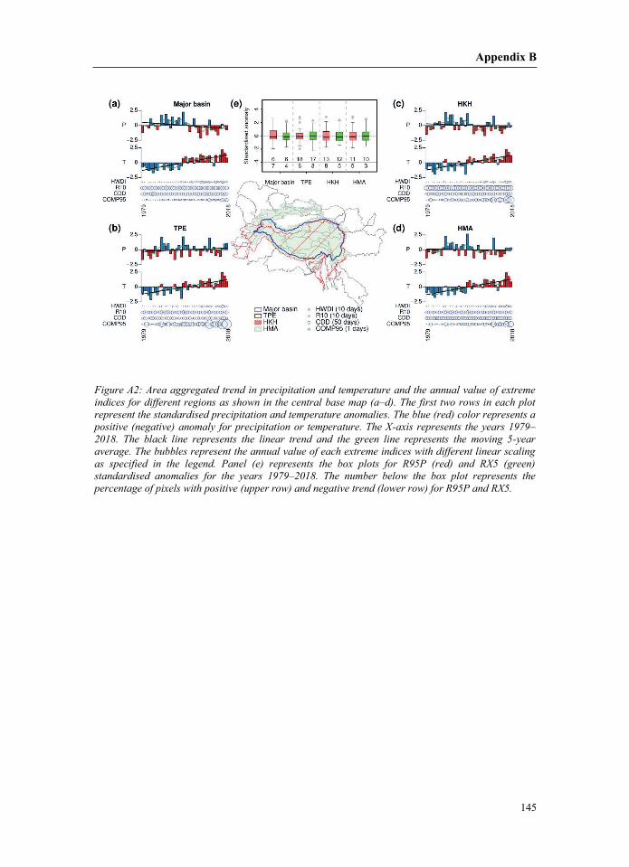
145
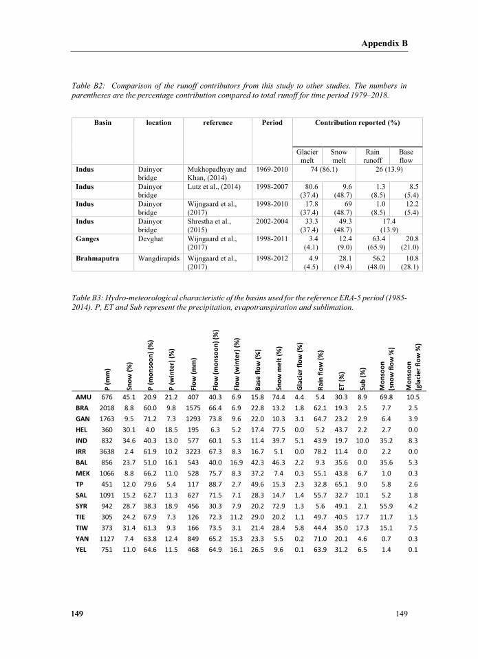
– – –

146
Appendix B
147
Appendix B
1
2
;
𝜎𝜎𝜎𝜎𝐹𝐹𝐹𝐹2 = ∑ [𝑑𝑑𝑑𝑑𝑑𝑑𝑑𝑑 (𝑥𝑥𝑥𝑥𝑖𝑖𝑖𝑖 … . 𝑥𝑥𝑥𝑥𝑛𝑛𝑛𝑛)
𝑑𝑑𝑑𝑑𝑥𝑥𝑥𝑥𝑖𝑖𝑖𝑖]
2𝜎𝜎𝜎𝜎𝑥𝑥𝑥𝑥𝑖𝑖𝑖𝑖
2𝑛𝑛𝑛𝑛
𝑖𝑖𝑖𝑖=1
(B1)
𝑥𝑥𝑥𝑥𝑖𝑖𝑖𝑖𝜎𝜎𝜎𝜎𝑥𝑥𝑥𝑥𝑖𝑖𝑖𝑖2
; –;;;–;
148
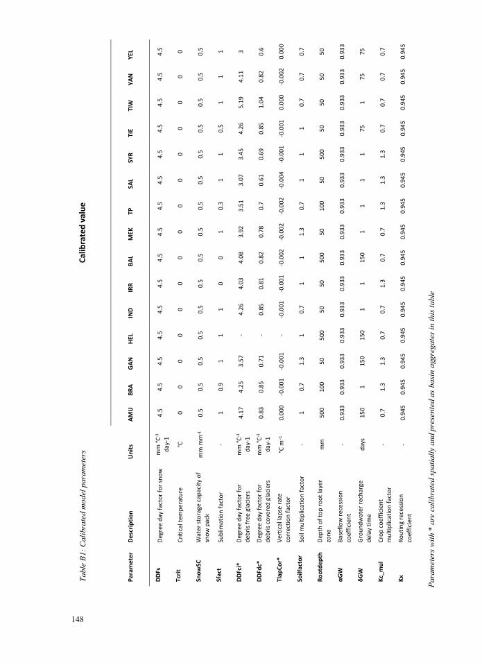
Calib
rate
d va
lue
YEL 4.5 0 0.5 1 3 0.6
0.00
0
0.7 50
0.93
3
75
0.7
0.94
5
YAN 4.5 0 0.5 1 4.
11
0.82
-0.0
02
0.7 50
0.93
3
75
0.7
0.94
5
TIW
4.5 0 0.5 1 5.
19
1.04
0.00
0
0.7 50
0.93
3
1 0.7
0.94
5
TIE 4.
5 0 0.5
0.5
4.26
0.85
-0.0
01
1 50
0.93
3
75
0.7
0.94
5
SYR 4.5 0 0.5 1 3.
45
0.69
-0.0
01
1 500
0.93
3
1 1.3
0.94
5
SAL 4.5 0 0.5 1 3.
07
0.61
-0.0
04
1 50
0.93
3
1 1.3
0.94
5
TP 4.5 0 0.5
0.3
3.51
0.7
-0.0
02
0.7
100
0.93
3
1 1.3
0.94
5
MEK
4.5 0 0.5 1 3.
92
0.78
-0.0
02
1.3 50
0.93
3
1 0.7
0.94
5
BAL 4.5 0 0.5 0 4.
08
0.82
-0.0
02
1 500
0.93
3
150
0.7
0.94
5
IRR 4.
5 0 0.5 0 4.
03
0.81
-0.0
01
1 50
0.93
3
1 1.3
0.94
5
IND 4.
5 0 0.5 1 4.
26
0.85
-0.0
01
0.7 50
0.93
3
1 0.7
0.94
5
HEL 4.5 0 0.5 1 - - - 1 500
0.93
3
150
0.7
0.94
5
GAN 4.5 0 0.5 1 3.
57
0.71
-0.0
01
1.3 50
0.93
3
150
1.3
0.94
5
BRA 4.5 0 0.5
0.9
4.25
0.85
-0.0
01
0.7
100
0.93
3
1 1.3
0.94
5
AMU
4.5 0 0.5 1 4.
17
0.83
0.00
0
1 500
0.93
3
150
0.7
0.94
5
Units
mm
°C-1
da
y-1
°C
mm
mm
-1
-
mm
°C-1
da
y-1
mm
°C-1
da
y-1
°C m
−1
- mm
-
days
- -
Desc
riptio
n
Degr
ee d
ay fa
ctor
for s
now
Criti
cal t
empe
ratu
re
Wat
er st
orag
e ca
pacit
y of
sn
ow p
ack
Subl
imat
ion
fact
or
Degr
ee d
ay fa
ctor
for
debr
is fre
e gl
acie
rs
Degr
ee d
ay fa
ctor
for
debr
is co
vere
d gl
acie
rs
Vert
ical l
apse
rate
co
rrec
tion
fact
or
Soil
mul
tiplic
atio
n fa
ctor
Dept
h of
top
root
laye
r zo
ne
Base
flow
rece
ssio
n co
effic
ient
Grou
ndw
ater
rech
arge
de
lay
time
Crop
coef
ficie
nt
mul
tiplic
atio
n fa
ctor
Rout
ing
rece
ssio
n co
effic
ient
Para
met
er
DDFs
Tcrit
Snow
SC
Sfac
t
DDFc
i*
DDFd
c*
Tlap
Cor*
Soilf
acto
r
Root
dept
h
αGW
δGW
Kc_m
ul
Kx
Appendix B
149149149
–
Basin location reference Period
P (m
m)
Snow
(%)
P (m
onso
on) (
%)
P (w
inte
r) (%
)
Flow
(mm
)
Flow
(mon
soon
) (%
)
Flow
(win
ter)
(%)
Base
flow
(%)
Snow
mel
t (%
)
Glac
ier f
low
(%)
Rain
flow
(%)
ET (%
)
Sub
(%)
Mon
soon
(s
now
flow
%)
Mon
soon
(g
lacie
r flo
w %
)
AMU 676 45.1 20.9 21.2 407 40.3 6.9 15.8 74.4 4.4 5.4 30.3 8.9 69.8 10.5 BRA 2018 8.8 60.0 9.8 1575 66.4 6.9 22.8 13.2 1.8 62.1 19.3 2.5 7.7 2.5 GAN 1763 9.5 71.2 7.3 1293 73.8 9.6 22.0 10.3 3.1 64.7 23.2 2.9 6.4 3.9 HEL 360 30.1 4.0 18.5 195 6.3 5.2 17.4 77.5 0.0 5.2 43.7 2.2 2.7 0.0 IND 832 34.6 40.3 13.0 577 60.1 5.3 11.4 39.7 5.1 43.9 19.7 10.0 35.2 8.3 IRR 3638 2.4 61.9 10.2 3223 67.3 8.3 16.7 5.1 0.0 78.2 11.4 0.0 2.2 0.0 BAL 856 23.7 51.0 16.1 543 40.0 16.9 42.3 46.3 2.2 9.3 35.6 0.0 35.6 5.3 MEK 1066 8.8 66.2 11.0 528 75.7 8.3 37.2 7.4 0.3 55.1 43.8 6.7 1.0 0.3 TP 451 12.0 79.6 5.4 117 88.7 2.7 49.6 15.3 2.3 32.8 65.1 9.0 5.8 2.6 SAL 1091 15.2 62.7 11.3 627 71.5 7.1 28.3 14.7 1.4 55.7 32.7 10.1 5.2 1.8 SYR 942 28.7 38.3 18.9 456 30.3 7.9 20.2 72.9 1.3 5.6 49.1 2.1 55.9 4.2 TIE 305 24.2 67.9 7.3 126 72.3 11.2 29.0 20.2 1.1 49.7 40.5 17.7 11.7 1.5 TIW 373 31.4 61.3 9.3 166 73.5 3.1 21.4 28.4 5.8 44.4 35.0 17.3 15.1 7.5 YAN 1127 7.4 63.8 12.4 849 65.2 15.3 23.3 5.5 0.2 71.0 20.1 4.6 0.7 0.3 YEL 751 11.0 64.6 11.5 468 64.9 16.1 26.5 9.6 0.1 63.9 31.2 6.5 1.4 0.1
Appendix B
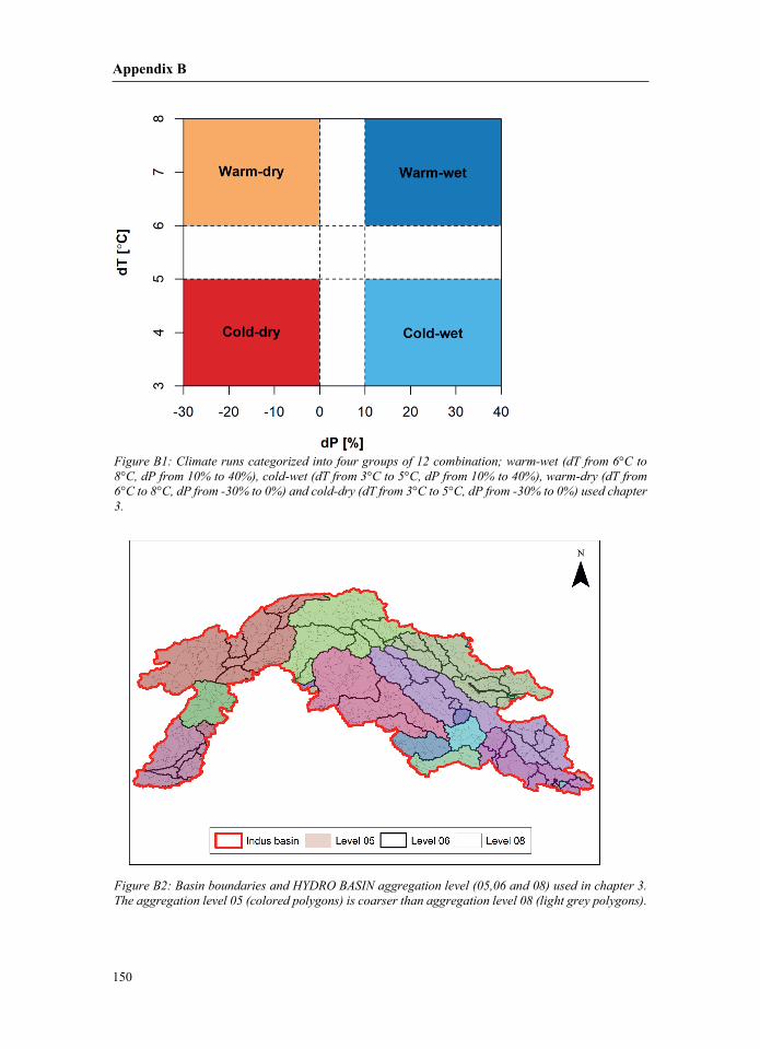
150
;
Appendix B
151
Appendix B
152
;
Appendix B
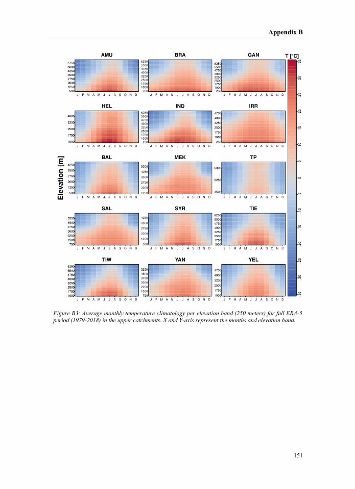
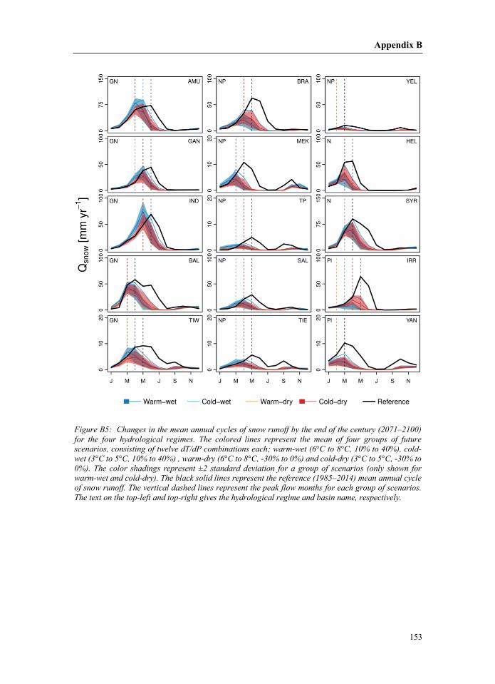
153
– ; –
Appendix B
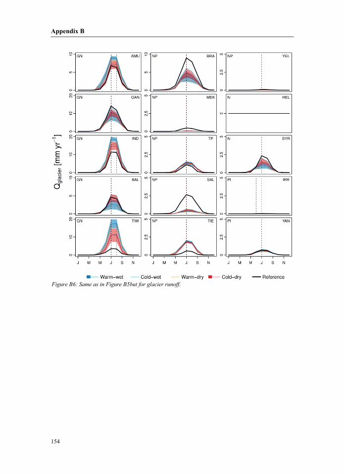
154
Appendix B
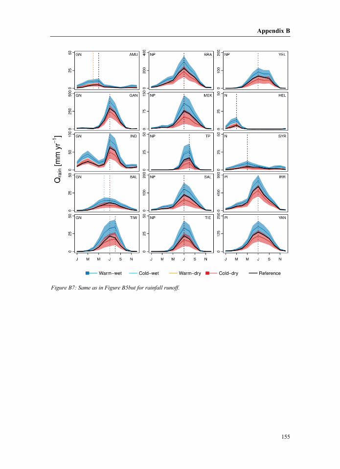
155
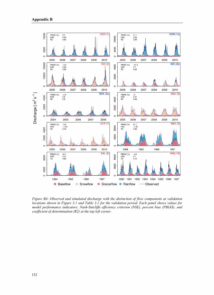
Appendix B
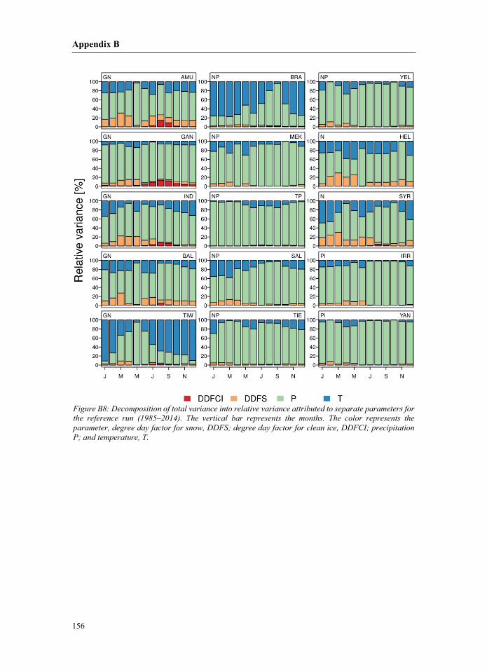
156
– ;;;
Appendix B
157
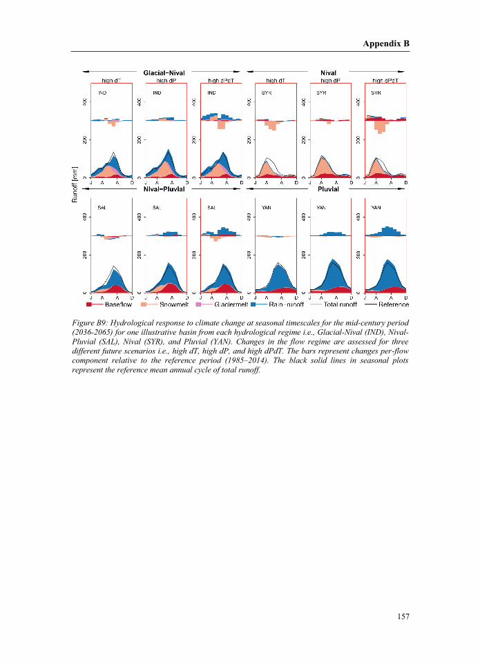
–
Appendix B
158
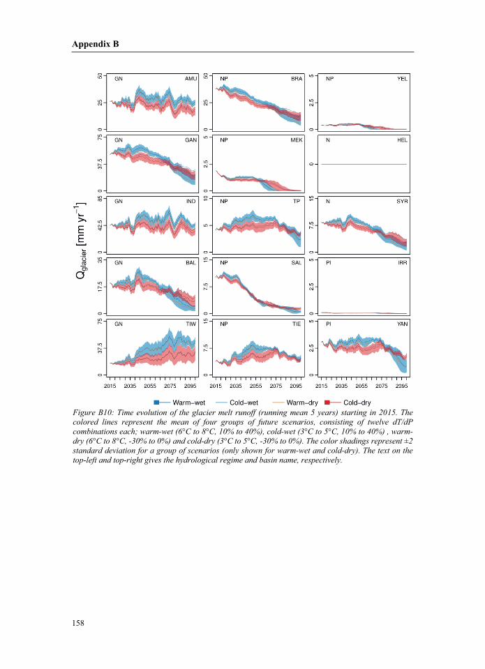
;
Appendix B
159
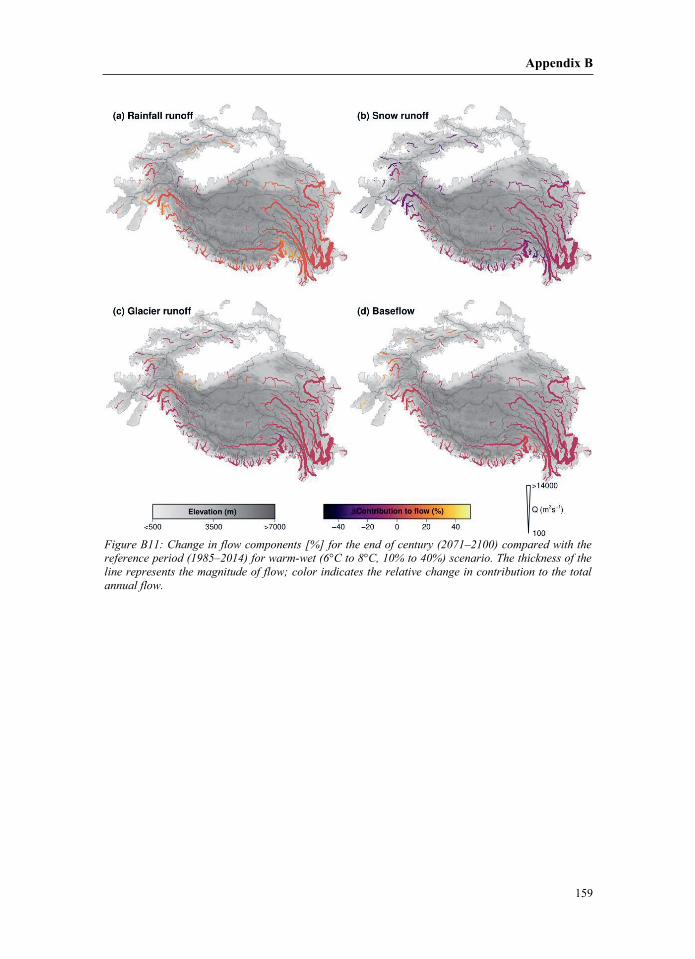
––;
Appendix B
160
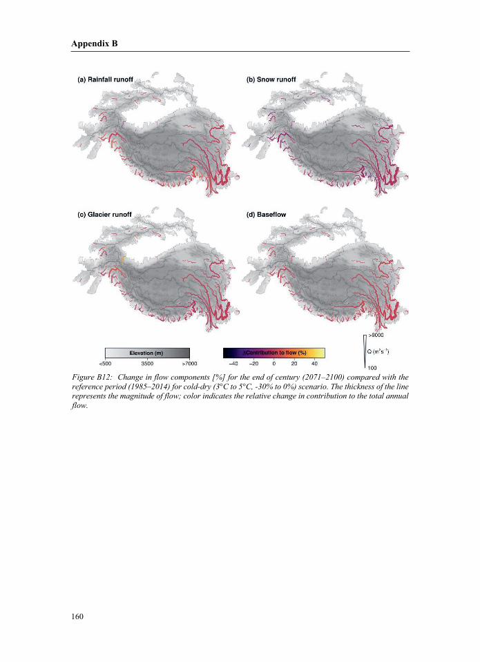
––;
Appendix C
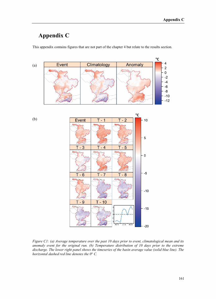
161
Appendix C
°C
°C
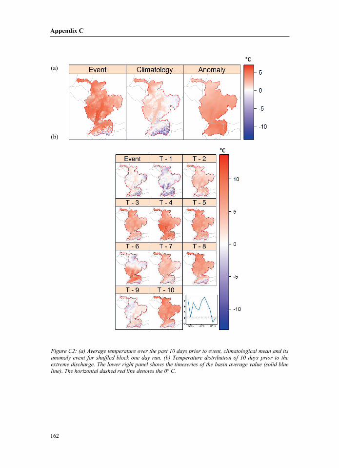
Appendix C
162
°C
°C
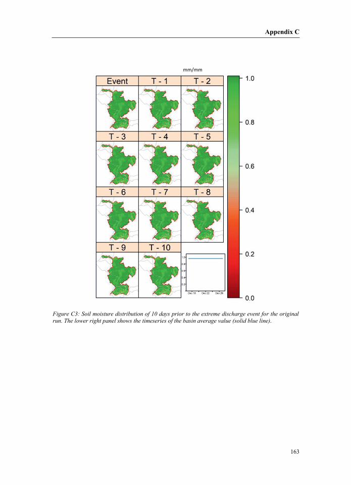
Appendix C
163
mm/mm
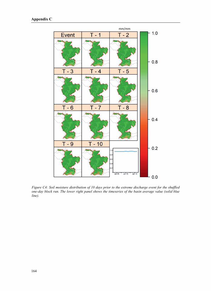
Appendix C
164
mm/mm
Appendix D
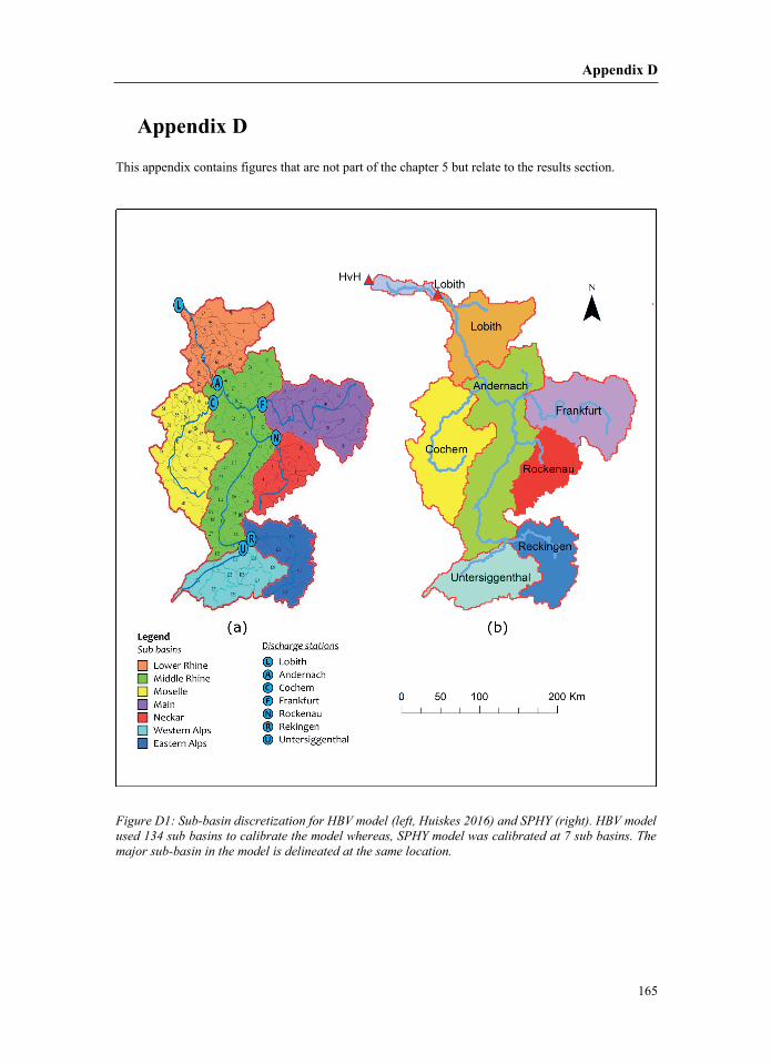
165
Appendix D
Appendix D
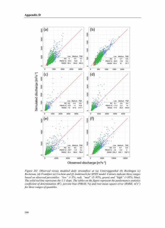
166
ed on observed percentiles: “low” (<5%, red), “med” (5–95%, green) and “high” (>95%, blue).
Appendix D
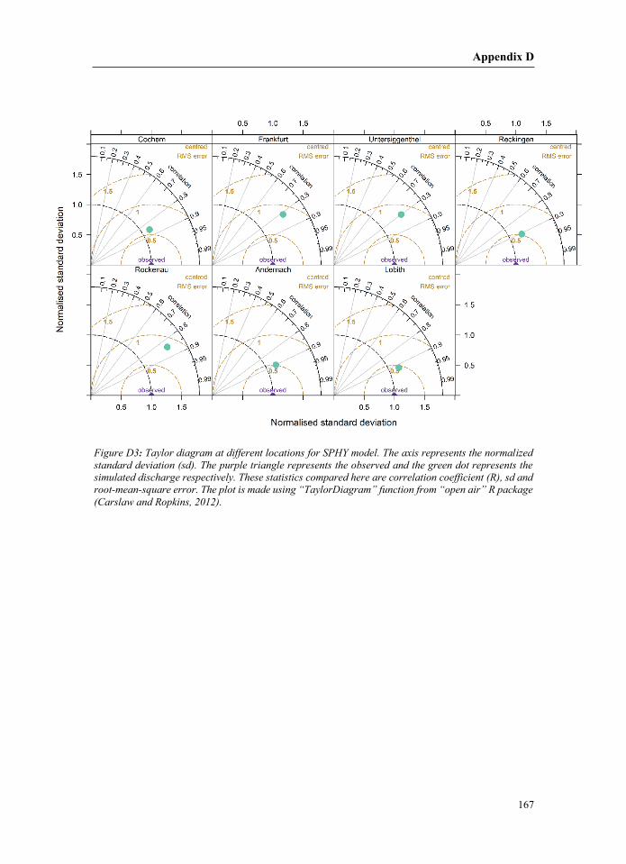
167
: ng “TaylorDiagram” function from “open air” R package
Appendix D
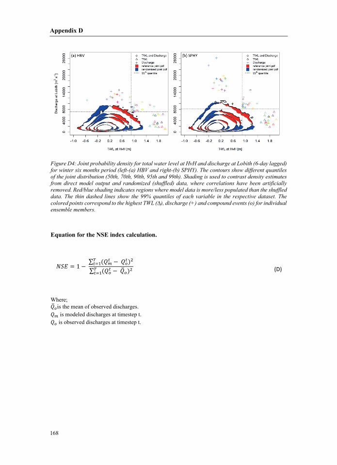
168
colored points correspond to the highest TWL (∆), discharge (+) and compound events (o) for individual
𝑁𝑁𝑁𝑁𝑆𝑆𝑆𝑆𝐸𝐸𝐸𝐸 = 1 − ∑ (𝑄𝑄𝑄𝑄𝑚𝑚𝑚𝑚
𝑡𝑡𝑡𝑡 − 𝑄𝑄𝑄𝑄𝑜𝑜𝑜𝑜𝑡𝑡𝑡𝑡 )2𝑇𝑇𝑇𝑇
𝑡𝑡𝑡𝑡=1∑ (𝑄𝑄𝑄𝑄𝑜𝑜𝑜𝑜
𝑡𝑡𝑡𝑡 − 𝑄𝑄𝑄𝑜𝑜𝑜𝑜)2𝑇𝑇𝑇𝑇𝑡𝑡𝑡𝑡=1
(D)
;𝑄𝑄𝑄𝑜𝑜𝑜𝑜𝑄𝑄𝑄𝑄𝑚𝑚𝑚𝑚𝑄𝑄𝑄𝑄𝑜𝑜𝑜𝑜
Bibliography
169
Bibliography
– –– –—––; flood risk in a warmer world, Earth’s Futur., 5(2), 171–– resolution history: Downscaling china’s climate from – – ––– Arcomano, T., Szunyogh, I., Pathak, J., Wikner, A., Hunt, B. R. and Ott, E.: A Machine Learning‐Based Global om glacier ice and seasonal snow in High Asia : separating melt water sources in river flow, ,
Bibliography
170
– – – Global Warming: An Emerging Hazard, Earth’s Futur., 7(4), 411––reams regulate the winter snow depth over the Tibetan Plateau ? North –––Barnard, P. L., Erikson, L. H., Foxgrover, A. C., Hart, J. A. F., Limber, P., O’Neill, A. C., van Ormondt, M., ––––– –– – ––
Bibliography
171
– –Beven, K.: Robert E. Horton’s perceptual model of infiltration processes, Hydrol. Proce– –– – ;;––––– –––––
Bibliography
172
–an, Č., Castellarin, A. and Chirico, G. B.: European floods, Science (80–Fackel, P., Amorim, I., Bělínová, M., Benito, G., Bertolin, C., , Lun, D., Panin, A., Parajka, J., Petrić, H., Rodrigo, F. S., Rohr, C., –Boer, F. D.: HiHydroSoil : A high resolution soil map of hydraulic properties (Version 1.2), Rep. Futur. 134, ––––– – – – ;– – – – –Brun, F.: Impact of the debris cover on High Mountain Asia glacier mass balances : a multi
Bibliography
173
– – ss of Debris‐Covered Glaciers, Geophys. Res. Lett., 48(6), doi:10.1029/2020gl092150, 2021. – ––– – –––nfo :: Portal of Knowledge for Water and Environmental Issues in Central Asia, [online] ––– –– –
Bibliography
174
–– –– – – – – Projected Precipitation Increases, Earth’s Futur., 7(8), 967–––; – –
Bibliography
175
aao – –– –– ––––D’Ippoliti, D., Michelozzi, P., Marino, C., De’Donato, F., Menne, B., Katsouyanni, K., Kirchmayer, U., Analitis, –– ––––– ––;–––– –
Bibliography
176
––––––– – – – ––– – G., Li‐Sha, L., Marengo, J., Mbatha, S., McGree, S., Menne, M., Milagros Skansi, M.F., Oonariya, C., Pabon‐Caicedo, J. D., Panthou, G., Pham, C., Rahimzadeh, Vazquez‐Aguirre, J., Vasquez, R., Villarroel, C., Vincent, L., Vischel, T., Vose, R. and Bin Hj Yussof, M. N.Development of an Updated Global Land In Situ‐Based Data Set of Temperature and Precipitation Extremes: –– – –Sagi, K. and Liebert, J.: HESS Opinions “should we apply bias imate model data?,” Hydrol. Earth Syst. Sci., 16(9), 3391–– – –
Bibliography
177
–––––––––––––; – – –––– ––
Bibliography
178
– – – From Riverine and Coastal Floods in Northwestern Europe, Earth’s Futur., 8(11), doi:10.1029/2020EF001752, ;– – ––––– –467, American Geophysical Union : Washington, D. C., 2013.–– –Theory and Statistics of Univariate Extremes : A Review To cite this version : HAL Id : halValue Theory and Statistics of Univariate Extremes : A Review, 2016.– –– – –
Bibliography
179
– –– – — –––––Hall, J., Arheimer, B., Borga, M., Brázdil, R., Claps, P., Kiss, A., Kjeldsen, T. R., Kriauĉun – ––––Hattermann, F. F., Krysanova, V. and Gosling, S. N.: Cross ‐ scale intercomparison of climate change i ––– ang, X., Severijns, C., Ştefǎnescu, S., Bintanja, R., Sterl, – –
Bibliography
180
– ––s covering Earth’s glaciers, Nat. Geosci., 13(9), 621–––– – – –––– ––H., Krauße, T., Kraft, P., Stoll, S., Bloschl, G. and Flühler, H.: Impact of modellers’ decisions on hydrological a – – – ; –
Bibliography
181
– –Huintjes, E., Sauter, T., Schroter, B., Maussion, F., Yang, W., Kropaček, J., Buchroithner, M., Scherer, – van Weele, M., de Winter, R. and van Zadelhoff, G.: KNMI’14: Climat– – – –– – Immerzeel, W. W. and Bierkens, M. F. P.: Asia’s water balance, Nat. Geosci., 5(12), 841–– – –– – –and vulnerability of the world’ –
Bibliography
182
– –– – –; –––– controls of geohazards induced by Nepal’s 2015 Go –– ––––
Bibliography
183
– –– Discharge : A Compound Event Analysis Using Ensemble Impact Modeling, Front. Earth Sci., 7(September), 1– ––– –––– – ––Klemeš, V.: The modelling of – – –––of the ten iterative steps in model development, Proc. iEMSs Third Bienn. Meet. “Summit Environ. Model. Software” (July 2006), (Step 2), 12, 2006.– –
Bibliography
184
– –;––– on Asia’s glaciers, Nature, 549, 257 [online] Available from: ––Kron, W.: Flood risk = hazard • values • vulnerability, Water Int., ––––bietes/Commission Internationale de l’Hydrologie du Bassin duRhin, 1999.– –– –
Bibliography
185
––study the world’s large river systems, Hydrol. Process., 27(15), 2171–– – –––– – –––– –– –– ––– –
Bibliography
186
–;––– – – –nsistent increase in High Asia’s runoff –Impacts on the Upper Indus Hydrology : Sources , Shifts and Extremes, , (November), – –– – – – – – – Kraaijenbrink, P., Malles, J. H., Maussion, F., Radić, V., Rounce, D. R., Sakai, A., Shannon, S., van de Wal, R. ons of Global Glacier Mass Change, Earth’s––––
Bibliography
187
he world’s highest weather stations on mou– –hydrological threshold events To cite this version : Temporal dynamics of hydrological threshold events, , 11(2), – – – Disciplinary Review, Earth’s Futur., 6(3–– – –– – – –– –– – –––– ––
Bibliography
188
– – ––– ––– – ;–– –Mudelsee, M., Borngen, M., Tetzlaff, G. and Grunewald, U.: No Upward Trends İn The OccurFloods İn Central Europe, Nature, 425(September), 166*169, 2003. ––– – Campen, H., Mason D’Croz, D., Van Meijl, H., Van Der – pierre, N., Berveiller, D., Gharun, M., Belelli Marchesini, L., Gianelle, D., Šigut, L., –– –
Bibliography
189
– –––;O’Go – –– – – ––––– –– –– – –– ––– –
Bibliography
190
– – – –esting for Haut Glacier d’Arolla, –– –––Pfahl, S., O’Gorman, P. A. and Fischer,– – – –;Pritchard, D. M. W., Forsythe, N., Fowler, H. J., O’Donnell, G. M. and Li, X. F.: Evalu––– ––
Bibliography
191
–– ––Rango, A. and Martinec, J.: Revisiting the Degree‐Day Method for Snowmelt Computations, JAWRA J. Am. – – ––––––– – ––––
Bibliography
192
– –l, M., Beaudoing, H. K., L’Ecuyer ––– –– ––– –Earth’s Futur., 8(3), doi:10.1029/2019EF001425, 2020. – ––––– – –
Bibliography
193
–– – – ––– ––;cient Based on Kendall’s Tau, J. Am. Stat. Assoc., 63(324), 1379–––––– ––reasing, Why Aren’t Floods?, –
Bibliography
194
––– – – – – – –––– ––;–;Research : Atmospheres, , 4889–––– –– d Storylines to Address Climate Risk, Earth’s Futur., 9(2), 1– –– –––
Bibliography
195
– ––– – ––––– – –––M., Wenninger, J. and Hoffmann, G.: HESS Opinions “a perspective on iso spiration to total evaporation,” Hydrol. Earth Syst. Sci., 18(8), 2815– – –––
Bibliography
196
–– –– – ––––– ––––– – – ––––, Martin, E., Masson, V., Guyomarc’H, G., Naaim –;Assessing the Hydrological Significance of the World’s Mountains, Mt. Res. Dev., ––
Bibliography
197
– – ––– –Wang, S. S. ‐Y., Kim, H., Coumou, D., Yoon, J., Zhao, L. and Gillies, R. R.: Consecutive extreme flooding and –, D.: WRF‐based dynamical downscaling of <scp>ERA5</scp> –– – – “Lothar” (2– –––
Bibliography
198
– ––– – – – – –– surface modeling: Meeting a grand challenge for monitoring Earth’s terrestrial ––;Wu, W., McInnes, K., O’Grady, J., Hoeke, R., Leonard, M. and Westra, S.: Mapping Dependence Between – ––––––––
Bibliography
199
– – ––– ––––– – Socioeconomic Changes, Earth’– – –– ––– – –––– –––
Bibliography
200
––––––– – – – – – –

201

202
Acknowledgements
203
Acknowledgements
‘guru’. Dear Bart

Acknowledgements
204
About the author
205
bachelor’s degree in Civil Engimaster’s in Water Resources During his master’s PhD was funded by Marie Skłodowska for “”

206
List of peer-reviewed publications
207
;
; ; ; ; ;
–
–
–
List of peer-reviewed publications
208
ICFM7 “”
Financial support
209
Marie Skłodowska project “ ” and


