Scheduling Tree-Dags Using FIFO Queues: AControl-Memory Tradeo�Sandeep N. BhattBell Communications ResearchMorristown, N.J. Fan R. K. ChungBell Communications ResearchMorristown, N.J.F. Thomson LeightonMITCambridge, Mass. Arnold L. RosenbergUniversity of MassachusettsAmherst, Mass.Abstract. We study a combinatorial problem that is motivated by \client-server" schedulersfor parallel computations. Such schedulers are often used, for instance, when computationsare being done by a cooperating network of workstations. Our results expose and quantify acontrol-memory tradeo� for such schedulers, when the computation being scheduled has thestructure of a binary tree. (Similar tradeo�s exist for trees of any �xed branching factor.) Thecombinatorial problem takes the following form. Consider, for integers k;N > 0, an algorithmthat employs k FIFO queues in order to schedule an N -leaf binary tree in such a way that eachnonleaf node of the tree is executed before its children. We establish a tradeo� between thenumber of queues used by the algorithm| which we view as measuring the control complexityof the algorithm| and the memory requirements of the algorithm, as embodied in the requiredcapacity of the largest-capacity queue. Speci�cally, for each integer k 2 f1; 2; : : : ; log2Ng, letQk(N) denote the minimax per-queue capacity for a k-queue algorithm that schedules N -leafbinary trees; let Q?k(N) denote the analogous quantity for complete binary trees. We establishthe following bounds: For general N -leaf binary trees, for all k,1k (2N � 1)1=klogN + 1 � Qk(N) � 2N1=k + 1:For complete binary trees, we derive tighter bounds. We prove that for all constant k,Q?k(N) = � N1=klog1�1=kN! :For general k, we obtain the following bounds:1k N1=k(logN + 1)1�1=k � Q?k(N) � (4k)1�1=k N1=klog1�1=kN :1

1 Introduction1.1 OverviewWe study the resource requirements of a class of algorithms for scheduling parallel com-putations. Our main results expose and quantify a tradeo� between two major resourcesof the algorithms, the complexity of their control mechanisms and their memory require-ments.The Computing Environment. We are interested in schedulers that operate in aclient-server mode, where the processors are the clients, and the scheduler is the server.One encounters such schedulers, for example, in systems that use networks of workstationsfor parallel computation; cf. [9], [10], [15]. We restrict attention to algorithms thatschedule static dags (directed acyclic graphs | which model the data dependencies in acomputation) in an architecture-independent fashion; cf. [1] - [3], [8], [11], [16] - [18]. Onecan view schedulers of this type as operating in the following way. (a) They determinewhen a task becomes eligible for execution (because all of its predecessors in the daghave been executed); (b) they queue up the eligible, unassigned tasks (in some way) ina FIFO process queue (PQ). When a processor becomes idle, it \grabs" the �rst task onthe PQ.Note that this scenario allows great latitude for processors: a processor can choose toparticipate or disappear from the computation independently at any time. But, once aprocessor accepts a task, it must complete the task within \unit time." In other words,the scheduler is clocked, and processors must commit to completing work they accept ata guaranteed rate.The Computational Load. Our particular focus is on dags that are binary treeswhose edges are oriented from the root toward the leaves. Such dags represent the datadependencies of certain types of branching computations. (We concentrate on binarytree-dags only for de�niteness; our results extend readily to tree-dags of arbitrary �xedbranching factor.)Formally, a binary tree dag (BT, for short) is a directed acyclic graph whose node-setis a pre�x-closed set of binary strings; i.e., for all binary strings x and all � 2 f0; 1g,if x� is a node of the BT, then so also is x. The null string (which, by pre�x-closure,belongs to every BT) is the root of the BT. Each node x of a BT has either two children,or one child, or no children; in the �rst case, the two children are nodes x0 and x1; inthe second case, the one child is either node x0 or node x1; in the last case, node x is aleaf of the BT. The arcs of a BT lead from each nonleaf node to (each of) its child(ren).For each ` 2 f0; 1; : : : ; ng, the node-strings of length ` comprise level ` of the BT (so the2

width = 5

BT: CBT:

Figure 1: A width-5, depth-6 BT and an 8-leaf depth-4 CBT.root is the unique node at level 0). The width of a BT is the maximum number of nodesat any level, and the depth of a BT is its number of levels.The (N = 2n)-leaf complete binary tree (CBT, for short) T n is the BT whose nodescomprise the set of all 2n+1 � 1 binary strings of length � n; hence the depth of T n isn + 1. There are N nodes at level n of T n, namely, its leaves, so the width of T n is N .See Fig. 1.Scheduling Regimens and Scheduler Structure. In order to establish rigorously atradeo� between the control complexity of our schedulers and their memory requirements,we must specify enough of the structure of a scheduler to quantify these resources. Weview a scheduler as using some number of FIFO queues to prioritize tasks that havebecome eligible for execution: the speci�c number of queues is our measure of the controlcomplexity of the scheduler; the minimax capacity of the queues is our measure of thescheduler's memory requirements.1 Roughly speaking, a scheduler uses its queues asfollows. As tasks get executed, they produce results that are necessary for the executionof their children. These results are loaded independently onto the FIFO queues of thescheduler; the task that is assigned to the next requesting processor is chosen from amongthose whose required input resides at the head of some queue.Multi-queue schedulers are interesting for our computational load because increasingthe number of queues within a scheduler allows one to proceed gradually from an eager1We recognize that one might wish to use data structures other than FIFO queues (e.g., LIFO stacks)to manage tasks awaiting execution; such alternatives also merit study.3

regimen, in which eligible tasks are delayed as little as possible before being assigned forexecution, to a lazy regimen, in which eligible tasks are delayed as long as possible beforebeing assigned for execution. The following facts about our framework will become clearas our study develops.� Any scheduler that uses only one queue:{ observes an eager regimen{ executes tree-nodes level by level, i.e., essentially in a breadth-�rst manner.� Lazy scheduling:{ is an option when the number of queues is commensurate with the length ofthe longest root-to-leaf path of the tree-dag{ is characterized by executing tree-nodes essentially in a depth-�rst manner.(The two uses of the quali�er \essentially" here re ect the fact that inputs for siblingtasks in the tree can be interchanged in the enqueuing process without any concomitantchange in the complexity of the scheduler.) While the control complexity of a schedulerincreases as it incorporates successively more queues, we shall show that the memoryrequirements | as measured by the maximum number of eligible tasks that are awaitingexecution | decrease concomitantly. We are able to establish and quantify this control-memory tradeo� rigorously.The Tradeo�. For positive integers k and N , let Qk(N) denote the minimax per-queue memory capacity for a k-queue algorithm that schedules N -leaf binary tree-dags;let Q?k(N) denote the analogous quantity for complete binary trees. We establish thefollowing bounds: For general BTs, for all k:21k (2N � 1)1=klogN + 1 � Qk(N) � 2N1=k + 1:Hence, the upper and lower bounds di�er by roughly a logarithmic factor. For completebinary trees, we derive tighter bounds: for all constant k:Q?k(N) = � N1=klog1�1=kN ! ;for general k: 1k N1=k(logN + 1)1�1=k � Q?k(N) � (4k)1�1=k N1=klog1�1=kN :This veri�es rigorously an instance of folklore in the scheduling community to the e�ectthat lazy dag-schedulers need less memory than do eager ones.2All logarithms are to the base 2. 4

1.2 The Formal ProblemBTs, being dags, represent the data-dependency graphs of computations, speci�callya class of branching computations. In this scenario, the nodes of the BT representthe tasks, while its arcs represent computational dependencies among the tasks. Thesedependencies in uence any algorithm that schedules the computation represented by theBT, in that a task-node cannot be executed until its parent task-node has been executed.This interpretation is consistent with the static (o�-line) scheduling problems studied in[1] - [3], [8], [11], [16] - [18].Scheduling BTs. The process of scheduling a BT T obeys the following rules. We aregiven an endless supply of enabling tokens and execution tokens. Placing an executiontoken on a node of T represents the process of executing the task represented by thenode. As we execute a node v of T , we place an enabling token on each arc that leaves v,to indicate that the results produced by v are now available; we label each enabling tokenwith a time stamp indicating when the token was placed. A node of T cannot receivean execution token until its incoming arc contains an enabling token. Thus, the processof scheduling a BT proceeds as follows: At step 0 of the scheduling process, we place anexecution token on the root of T (which, of course, has no incoming arc), and we placean enabling token with time stamp 0 on each arc leaving the root. At each subsequentstep, say step s > 0, we perform two actions:� We place an execution token on some (one) unexecuted node of T whose incomingarc contains an enabling token.� We place enabling tokens, with time stamp s, on all arcs that leave the just-executednode.This process continues until all nodes of T contain execution tokens. The reader shouldbe able to extrapolate from this BT-speci�c description to a description of a schedulingprocess for an arbitrary dag: the major di�erence is that a node cannot be executed untilall of its incoming arcs contain enabling tokens.We call a scheduling algorithm eager if, at each step, it places an execution token onan unexecuted node whose incoming arc contains an enabling token having as small atime-stamp as possible; we call a scheduling algorithm lazy if, at each step, it places anexecution token on an unexecuted node whose incoming arc contains an enabling tokenhaving as large a time-stamp as possible. One veri�es easily that an eager schedulingalgorithm executes the nodes of T level by level, i.e., essentially in a breadth-�rst manner,while a lazy scheduling algorithm executes the nodes of T essentially in a depth-�rstmanner. Our interest here is in a family of scheduling algorithms that form a progression5

between eager scheduling at one extreme and lazy scheduling at the other. We need moretools to describe this progression formally.Scheduling BTs using Queues: Control vs. Memory. The reader can verify easilythat the process of scheduling a BT T is \isomorphic" to the process of topologicallysorting T , i.e., linearly ordering the nodes of T so that each nonleaf node precedesits children. Our study focuses on the structure of the algorithm that \manages" theprocess of scheduling/topologically sorting T . The particular formal framework for ourstudy specializes the framework studied in [4] - [7], [13].A k-queue scheduler for a BT T proceeds as follows. Initially, at time 0, the schedulerexecutes the root of T and enqueues each arc that leaves the root, independently, in oneof its k queues. Inductively, a node v of T is eligible to be executed | i.e., to receivean execution token | just when its entering arc is at the head (i.e., the exit port) ofsome queue. As the scheduler executes a node v, it dequeues the arc that enters v;simultaneously | as part of the same atomic action | the scheduler enqueues each arcthat leaves v, independently, on one of the k queues. Henceforth, let us denote the kqueues of the scheduler as queue #1, : : :, queue #k.A multi-queue BT-scheduler uses its queues to manage the eligible tasks that areawaiting execution. Speci�cally, enqueuing an arc is equivalent to endowing it with anenabling token; dequeuing an arc is equivalent to placing an execution token on the nodethe arc enters. The \management" function of the queues is manifest in the fact thatonly nodes whose incoming arcs reside at the heads of queues can be executed in thenext step.Easily, there exist k-queue BT-schedulers for every positive integer k. A straight-forward induction veri�es that there is a unique 1-queue BT-scheduler | up to thedistinction between \left" and \right" children.Fact 1.1 The unique 1-queue BT-scheduler executes BT-nodes level by level, i.e., \es-sentially" in breadth-�rst order.A consequence of the rules for manipulating queues is that the arc that enters a BT-node v does not get enqueued until all of the ancestors of v have already been executed.This veri�es the following simple observation, which is important later.Fact 1.2 All arcs that coexist in the queues of a multiqueue BT-scheduler at any instantenter nodes that are independent in the BT; i.e., none is an ancestor of another.We view the number of queues a BT-scheduler uses as its control complexity; we viewthe worst-case individual capacity of the queues as measuring the memory requirements6

of the scheduler. In this worldview, the capacity of queue #q is the maximum numberof arcs of T that will ever reside in queue #q at the same instant. Clearly, the worst-case cumulative capacity of the queues | which some might view as a better measureof a scheduler's memory requirements | is at most k times the worst-case individualcapacity. Obtaining bounds on the cumulative capacity that are tighter than the oneobtained from this simple observation appears to be quite di�cult.We now turn to the topic of tradeo�s between the amount of control in a BT-schedulerand its memory requirements.2 A Control-Memory Tradeo�A Roadmap. Our goal is to verify the tradeo�s that are stated roughly at the end ofSection 1.1, between the control complexity of a BT-scheduler | as measured by thequantity k | and the memory requirements of the scheduler | as measured by thequantities Qk(N) and Q?k(N). The possible existence of such a tradeo� is suggested bya family of simple CBT-schedulers (using successively more queues) that we present andanalyze in Section 2.1. This family of schedulers, which derives from [7], illustrates thatQ?k(N) = O(N1=k), uniformly in N and k. In Section 2.2, we state formally the actualtradeo�s that are the main contribution of our study. Sections 3 and 4 are devoted toproving the upper bounds in the tradeo�s for general BTs and complete BTs, respectively;Section 5 is devoted to proving the lower bounds of the tradeo�s. We note in Section 6.1that our results extend readily to other classes of tree-based dags. Although we cannotcharacterize what non-tree-based dags experience such tradeo�s, we close the paper withremarks in Section 6.2 about characteristics of classes of dags that preclude such tradeo�s.Since our upper and lower bounds derive from recurrences on Qk(N) and Q?k(N) asfunctions of k and N , it is useful to note the following immediate consequence of Fact1.1.Lemma 2.1 Consider a 1-queue scheduling algorithm for an N-leaf, width-W , depth-DBT.(a) The queue of the scheduler must have capacity at least W � (2N � 1)=D.(b) It su�ces for the queue of the scheduler to have capacity W � N .(c) In particular, for all N = 2n, Q?1(N) = N .2.1 A Simple Recursive CBT-Schedule AlgorithmA k-Queue CBT-Scheduler 7

Input: the (N = 2n)-leaf CBT T n1. Schedule the top d(n+ 1)=ke levels of T n using queue #k.2. For each \leaf" of the tree scheduled in step 1, in turn, schedule the CBT rooted atthat \leaf" by using queues #1; : : : ;#(k�1) to execute recursively the (k�1)-queueversion of this algorithm.See Fig. 2.Analyzing the Algorithm. Since each queue is used to schedule (possibly many)CBT(s) of height (logN + 1)=k, no queue need have capacity greater than dN1=ke. Asan immediate consequence, we have:Fact 2.1 For all positive integers N = 2n and k � n,Qk(N) � dN1=ke: (1)Note that when k = logN in this family of algorithms, each queue has constantcapacity. At this point, the queues are collectively simulating the action of a single stack,executing the CBT in a depth-�rst, hence lazy, regimen. (One can verify by a simpleadaptation of the argument in [12] that the cumulative capacity of the queues whenk = logN cannot be improved by more than a constant factor.)2.2 The Real Control-Memory Tradeo�sThe possible tradeo� suggested in Fact 2.1 (i.e., the possibility that there exist lowerbounds that come close to the upper bounds (1)) does indeed exist. In the next threesections we prove the following bounds, which are re�nements of the rough bounds wehave stated earlier.A. The Upper Bound for General BTsIn Section 3, we show that the upper bound (1) holds for arbitrary BTS, to within afactor of 2.Theorem 2.1 For all positive integers N and k � logN , the minimax per-queue capacityof algorithms that use k queues to schedule an N-leaf BT satis�esQk(N) � 2N1=k + 1 � (1=2)N1�1=k � 2N1=kbN1�1=kc : (2)8

use queue #k

#1 − #(k−1)

use queues

(n+1)/k

(n+1)(1 − 1/k)

Figure 2: An indication of queue utilization in a capacity-saving two-queue schedule forthe 2n-leaf CBT. 9

B. The Upper Bound for Complete BTsIn Section 4, we demonstrate that, somewhat surprisingly, the upper bound (1) can beimproved for complete BTs.Theorem 2.2 For all positive integers N = 2n and k � n, the minimax per-queuecapacity of algorithms that use k queues to schedule the N-leaf CBT satis�esQ?k(N) � (4k)1�1=k N1=klog1�1=kN : (3)C. The Lower BoundsOur lower bounds for scheduling BTs derive from the following bound which is proved inSection 5. For positive integers k,W , and D, letQ0k(W;D) denote the minimax per-queuecapacity when k queues are used to schedule a BT having width W and depth � D.Theorem 2.3 Let T be an N-leaf BT having width W and depth D. For all k � logN :given any k-queue algorithm that schedules T , at least one queue must have capacityQ0k(W;D) � � 1k!2k�1�1=k W 1=kD1�1=k : (4)Since W � (2N � 1)=D for an N -leaf BT having width W and depth D, Theorem2.3 immediately yieldsCorollary 2.1 (The Lower Bound for General BTs)Let T be an N-leaf, depth-D BT. For all k � logN : given any k-queue algorithm thatschedules T , at least one queue must have capacity no smaller than� 1k!2k�1�1=k (2N � 1)1=kD � 1k (2N � 1)1=kD :Since there exist N-leaf BTs of depth logN + 1, it follows thatQk(N) � 1k (2N � 1)1=klogN + 1 :Since an (N = 2n)-leaf CBT has width W = N and depth D = n + 1, we get astronger corollary of Theorem 2.3 for CBTs.10

Corollary 2.2 (The Lower Bound for Complete BTs)For all positive integers N = 2n and k � n: given any k-queue algorithm that schedulesthe N-leaf CBT, at least one of the queues must have capacityQ?k(N) � 1k N1=k(logN + 1)1�1=k :Corollaries 2.1 and 2.2 yield the claimed lower bounds on Qk(N) and Q?k(N), respec-tively.D. The Fixed-k Tradeo� for Complete BTsIt is worth remarking that for �xed k, the bounds of Theorems 2.2 and Corollary 2.2 arewithin constant factors of each other.Corollary 2.3 For any �xed constant k, there exist positive constants c1 and c2 suchthat, for all N = 2n, c1 N1=klog1�1=kN � Q?k(N) � c2 N1=klog1�1=kN :3 The Upper Bounds for General BTsThis section is devoted to proving the upper bounds of Theorem 2.1, via a recursivefamily of BT-scheduling algorithms that match the memory requirements of the CBT-scheduling algorithms of Section 2.1 (to within constant factors). Let us be given anN -leaf BT T .Preprocessing. Label each arc of T with the number of leaves in the sub-BT of T rootedat the node that the arc enters. This can be accomplished using either an O(N)-timesequential algorithm or an O(logN)-time parallel algorithm, depending on the resourcesavailable to the scheduler.3.1 The k-Queue AlgorithmUse queue #k to start executing the nodes of T , from the root, level by level. As thescheduler executes a node v that has two children, it scans the labels of the arcs leavingv. 11

� If the label of one arc leaving v is > b12N1�1=kc, and the label of the other arcleaving v is � b12N1�1=kc, then the scheduler1. enqueues the arc leading to the big subtree in queue #k2. immediately schedules the smaller subtree, using queues #1; : : : ;#(k � 1) ina recursive invocation of the (k � 1)-queue version of this algorithm.� If the labels of both arcs leaving v are � b12N1�1=kc, and the label of the arc enteringv is > b12N1�1=kc, then the scheduler immediately schedules the subtree rooted atnode v, using queues #1; : : : ;#(k�1) in a recursive invocation of the (k�1)-queueversion of this algorithm.3.2 Analyzing the k-Queue AlgorithmIn order to assess the memory requirements of the algorithm, we isolate the portionsof the scheduled tree T that are executed under the control of each of the k queues.Speci�cally, in order to bound the capacity of queue #k, we prune it by removing allsubtrees that are processed using queues #1; : : : ;#(k � 1). We claim that the prunedversion of T has no more than2N1=k + 1� (1=2)N1�1=k � 2N1=kbN1�1=kcleaves. In order to see this, note that the \leaves" of the pruned version of T all haveincoming arcs with labels > b12N1�1=kc, meaning that the subtree rooted at each of these\leaves" has > b12N1�1=kc leaves. Since T has N leaves in all, this bound on the numberof leaves in each of the removed subtrees implies that there are fewer thanNb(1=2)N1�1=kc (5)removed subtrees. But, the roots of these subtrees comprise the \leaves" of the prunedversion of T , and it is the pruned version which is the tree scheduled using queue #k.The claimed capacity of queue #k now follows from Lemma 2.1 and elementary boundsfor the fraction (5).In order to bound the capacities of queues #1; : : : ;#(k� 1), note that each recursiveinvocation of the algorithm using those queues schedules a BT having no more thanbN1�1=kc leaves. It follows thatQk(N) � max 2N1=k + 1 � (1=2)N1�1=k � 2N1=kbN1�1=kc ; Qk�1(bN1�1=kc)! ;whence the Theorem. 12

4 The Upper Bounds for Complete BTsThis section is devoted to proving the upper bound of Theorem 2.2, via a recursive familyof CBT-scheduling algorithms that have better memory requirements than the family ofschedulers of Section 2.1.For purely technical reasons, our algorithmic strategy inverts the question we reallywant to solve. Speci�cally, instead of starting with a target number N of leaves andasking how small a queue-capacity is su�cient to schedule an N -leaf CBT, we start witha target queue-capacity Q and ask how large a CBT we can schedule using queues ofcapacity Q. We proceed, therefore, by considering the quantity N k(Q) which denotesthe maximum number of leaves in a CBT that can be scheduled using k queues, each ofcapacity Q. By deriving a lower bound on the quantity N k(Q), we can infer an upperbound on the dual quantity Q?k(N). In order to avoid a proliferation of oors and ceilingsin our calculations, we assume henceforth that Q is a power of 2; this assumption will beseen to a�ect only constant factors.Since the algorithm that establishes the general case of Theorem 2.2 is somewhatcomplex, we present �rst the algorithm for the case of two queues (k = 2), which alreadyexposes the subtlest ideas in the general algorithm.4.1 The Case k = 2Our two-queue CBT-scheduling algorithm operates in three phases which we describenow in rough terms. Let �(Q) =def blog(logQ � 1)c. In the �rst phase, the algorithmuses queue #2 to schedule (the execution of) the top �(Q)+ 1 levels of a CBT, retainingthe \leaves" from the last level in the queue. In the second phase, the algorithm staggersexecuting these \leaves" (hence, removing them from queue #2) with beginning to usequeue #1 to schedule the middle logQ� 1 levels of the CBT. By the end of the secondphase, queue #2 has been emptied, hence is available for reuse. In the third phase, thealgorithm staggers using queue #1 to schedule the remainder of the middle logQ � 1levels of the CBT with using queue #2 to schedule the bottom logQ levels. This latterstaggering proceeds by having queue #2 schedule a Q-leaf CBT rooted at each middle-tree \leaf" from queue #1. To assist the reader in understanding the ensuing detaileddescription of the algorithm, we depict in Fig. 3 the ultimate usage pattern of the twoqueues.A. An E�cient Two-Queue CBT-Scheduling AlgorithmPhase 1: The Top of the Tree.In this phase, we use queue #2 to schedule (the execution of) the top �(Q) + 1 levels13

log h −1

h−1

h

QUEUE #2

QUEUE #1QUEUE #1

#2 #2 #2 #2Figure 3: The target utilization of two capacity-Q queues when scheduling the executionof a \big" CBT; h = logQ.14

TOP TREE

log log Q − 1

Last level:

NODES REMAINING IN QUEUE #2Figure 4: Scheduling the execution of the top of the CBT.of the CBT we are scheduling, using the breadth-�rst regimen that is the unique way asingle queue can schedule a CBT (cf. Fact 1.1). At the end of this phase, queue #2 willcontain 2�(Q) nodes. We make the transition into Phase 2 of the algorithm by consideringeach node in queue #2 as the root of a \middle" CBT (which will have Q=2 \leaves").See Fig. 4.Phase 2: The Middle of the Tree.In this phase, we use queue #1 to schedule (the execution of) the middle trees thatcomprise the next logQ � 1 levels of the CBT we are scheduling. This is the mostcomplicated of the three phases, in that these middle trees get executed in a staggeredmanner, in two senses. First, the executions of the 2�(Q) middle trees get interleaved inthe schedule we are producing. Second, the execution of the middle trees is interleavedwith segments of Phase 3, wherein the bottom trees are executed.We describe �rst the initial portion of Phase 2, i.e., the portion before the phase getsinterrupted by segments of Phase 3.Execute the �rst node from queue #2, which is level 0 (i.e., the root) of the �rstmiddle tree; place the children of this node in queue #1. Next, proceed through thefollowing iterations; see Fig. 5.Step 1. Begin the �rst middle tree. 15

0 1

1 1 22

2 2 2 2

3 3 3 3 3 3 3 3

3 3 3 3

3 3

2

Figure 5: The initial steps of Phase 2.16

Step 1.1. Use queue #1 to schedule the execution of level 1 of the �rst middletree.Step 1.2. Execute the root (level 0) of the second middle tree (removing that nodefrom queue #2); place the children of this root in queue #1.Step 2. Continue the �rst middle tree; begin the second middle tree.Step 2.1. Use queue #1 to schedule the execution of level 2 of the �rst middletree.Step 2.2. Use queue #1 to schedule the execution of level 1 of the second middletree.Step 2.3. Execute the root (level 0) of the third middle tree (removing that nodefrom queue #2); place the children of this root in queue #1.Step 3. Continue the �rst and second middle trees; begin the third middle tree.Step 3.1. Use queue #1 to schedule the execution of level 3 of the �rst middletree.Step 3.2. Use queue #1 to schedule the execution of level 2 of the second middletree.Step 3.3. Use queue #1 to schedule the execution of level 1 of the third middletree.Step 3.4. Execute the root (level 0) of the fourth middle tree (removing that nodefrom queue #2); place the children of this root in queue #1.� � �Step (2�(Q) � 1). Finish the �rst middle tree; continue the second through next-to-lastmiddle trees; begin the last middle tree.Step (2�(Q) � 1).1. Use queue #1 to schedule the execution of level logQ � 2 ofthe �rst middle tree.Step (2�(Q) � 1).2. Use queue #1 to schedule the execution of level logQ � 3 ofthe second middle tree.� � �Step (2�(Q) � 1).(2�(Q) � 1). Use queue #1 to schedule the execution of level 1 ofthe second from last middle tree.Step (2�(Q) � 1).(2�(Q)). Execute the root (level 0) of the last middle tree (re-moving that node from queue #2); place the children of this root in queue#1. 17

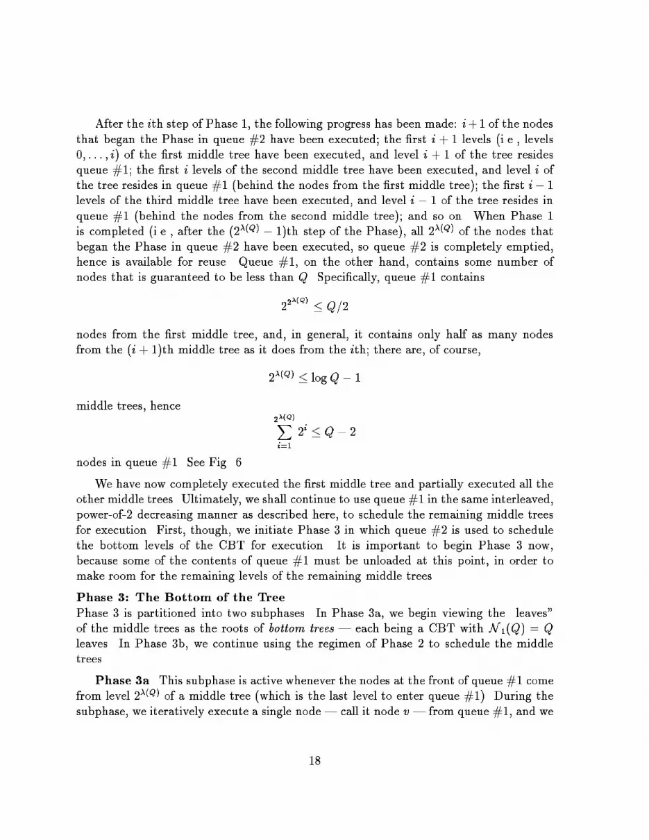
After the ith step of Phase 1, the following progress has been made: i+1 of the nodesthat began the Phase in queue #2 have been executed; the �rst i + 1 levels (i.e., levels0; : : : ; i) of the �rst middle tree have been executed, and level i + 1 of the tree residesqueue #1; the �rst i levels of the second middle tree have been executed, and level i ofthe tree resides in queue #1 (behind the nodes from the �rst middle tree); the �rst i� 1levels of the third middle tree have been executed, and level i � 1 of the tree resides inqueue #1 (behind the nodes from the second middle tree); and so on. When Phase 1is completed (i.e., after the (2�(Q) � 1)th step of the Phase), all 2�(Q) of the nodes thatbegan the Phase in queue #2 have been executed, so queue #2 is completely emptied,hence is available for reuse. Queue #1, on the other hand, contains some number ofnodes that is guaranteed to be less than Q. Speci�cally, queue #1 contains22�(Q) � Q=2nodes from the �rst middle tree, and, in general, it contains only half as many nodesfrom the (i+ 1)th middle tree as it does from the ith; there are, of course,2�(Q) � logQ� 1middle trees, hence 2�(Q)Xi=1 2i � Q� 2nodes in queue #1. See Fig. 6.We have now completely executed the �rst middle tree and partially executed all theother middle trees. Ultimately, we shall continue to use queue #1 in the same interleaved,power-of-2 decreasing manner as described here, to schedule the remaining middle treesfor execution. First, though, we initiate Phase 3 in which queue #2 is used to schedulethe bottom levels of the CBT for execution. It is important to begin Phase 3 now,because some of the contents of queue #1 must be unloaded at this point, in order tomake room for the remaining levels of the remaining middle trees.Phase 3: The Bottom of the Tree.Phase 3 is partitioned into two subphases. In Phase 3a, we begin viewing the \leaves"of the middle trees as the roots of bottom trees | each being a CBT with N 1(Q) = Qleaves. In Phase 3b, we continue using the regimen of Phase 2 to schedule the middletrees.Phase 3a. This subphase is active whenever the nodes at the front of queue #1 comefrom level 2�(Q) of a middle tree (which is the last level to enter queue #1). During thesubphase, we iteratively execute a single node | call it node v | from queue #1, and we18

TOP TREE

MIDDLE TREES

level h−1

level h−2

level 1

log h − 1 leaves

in queue #1

in queue #1

in queue #1Figure 6: The situation after Phase 2.19

TOP TREE

BOTTOM TREES

MIDDLE TREES

level h−2

level h−1

(h levels each)

level 1

log h − 1 leaves

in queue #1

in queue #1

in queue #1

Figure 7: The situation after Phase 3a begins: the �rst two bottom trees have been exe-cuted. 20

use queue #2 to schedule the CBT on Q leaves rooted at node v (using the breadth-�rstregimen, of course). See Fig. 7.Phase 3b. This subphase is active whenever the nodes at the front of queue #1 donot come from level 2�(Q) of a middle tree. During the subphase, we perform one morestep of Phase 2, to extend the executed segment of the middle tree. To illustrate ourintent, the instance of Subphase 3b that is executed immediately after the �rst round ofexecutions of Subphase 3a (wherein the leftmost Q=2 bottom trees are executed) has thefollowing form.Step (2�(Q) + 1). Finish the second middle tree; continue the third through last middletrees.Step (2�(Q) + 1).1. Use queue #1 to schedule the execution of level 2�(Q) of thesecond middle tree.Step (2�(Q) + 1).2. Use queue #1 to schedule the execution of level 2�(Q) � 1 ofthe third middle tree.� � �Step (2�(Q) + 1).(2�(Q) � 1). Use queue #1 to schedule the execution of level 2 ofthe second from last middle tree.Step (2�(Q) + 1).(2�(Q)). Use queue #1 to schedule the execution of level 1 of thelast middle tree.See Fig. 8.B. The AnalysisCorrectness being (hopefully) clear, we need only assess how much CBT we are gettingfor given queue-capacity Q. There are2�(Q) > 12(logQ� 1)top-tree leaves, hence, at least 14Q(logQ�1) middle-tree leaves, hence at least 14Q2(logQ�1) CBT leaves. It follows that N 2(Q) � 14Q2(logQ� 1):Inverting this inequality to obtain the desired upper bound on Q?2(N), we �nd thatQ?2(N) � 2 NlogN !1=2 :21

TOP TREE

BOTTOM TREES

MIDDLE TREES

h−1 levels level h−1

level 2

log h − 1 leaves

(h levels each)

in queue #1

in queue #1

Figure 8: The situation after Phase 3b begins: the �rst set of bottom trees have beenexecuted; the second middle tree has been completed.22

4.2 The Case of General kWe now show how to generalize our two-queue CBT-scheduler to obtain multiqueueCBT-schedulers for arbitrary numbers of queues.A. The AlgorithmOur k-queue CBT-scheduling algorithm uses Phases 1, 2, and 3b of our two-queuescheduling algorithm directly. It modi�es only Phase 3a, in the following way.Phase 3a. This subphase is active whenever the nodes at the front of queue #1 comefrom level logQ� 2 of a middle tree (which is the last level to enter queue #1). Duringthe subphase, we iteratively execute a single node | call it node v | from queue #1,and we use queues #2; : : : ;#k to schedule a CBT on Q leaves, rooted at node v, usinga recursive invocation of the (k � 1)-queue version of this algorithm.Note that the two-queue CBT-scheduler of the previous subsection can, in fact, beobtained via this recursive strategy, from the base case k = 1.As with the case k = 2, queues #2; : : : ;#k are all available for this recursive callbecause: (a) the last \leaf" of the top tree is extracted from queue #2 for executionjust before the �rst \leaf" of the leftmost middle tree is extracted from queue #1 forexecution; (b) queues #3; : : : ;#k are not used at all with the top or middle trees abovethis level of the �nal CBT.B. The AnalysisCorrectness being (hopefully) obvious, we need consider only how many leaves the CBTwe have scheduled has, as a function of the given queue-capacity Q. Because each recur-sive call to our CBT-scheduler generates its own \top" tree and its own set of \middle"trees, but uses one fewer queue than the previous call, it is not hard to verify that thisnumber is given by the recurrenceN 1(Q) = QN k+1(Q) � 14Q(logQ� 1)N k(Q)Easily, this system yields the following solution, which holds for all k � 1.N k(Q) � Q�14Q logQ�k�1 :For our ends, we invert this relation, to get the sought upper bound on Q?k(N). 223

5 The Lower Bounds in the Tradeo�This section is devoted to proving the lower bound in Theorem 2.3.Let us be given an N -leaf BT T having width W and depth D. Call a level of Tthat has W nodes a wide level. Consider the action of an arbitrary k-queue schedule forexecuting T .Our analysis of the given schedule is based on parsing the sequence of node-executionsprescribed by the schedule into phases. Recall that the action of executing a node andloading its outgoing arcs into queues is a single atomic action.De�ne Phase 0 to be that part of the process wherein the root of T (which must bethe �rst node in the schedule) is executed and its outgoing arcs loaded onto queues.Inductively, de�ne Phase i + 1 to be that part of the process that completes theexecution of all nodes whose incoming arcs were loaded into queues during Phase i. Inother words, Phase i + 1 continues as long as some queue still contains an arc that wasput there during Phase i; the Phase ends when the last of these Phase-i \legacies" hasbeen executed.One veri�es by a straightforward induction that all nodes on level i of T must havebeen executed by the end of Phase i. The following Fact is an immediate consequence ofthis inference.Fact 5.1 There are at most D phases in the sequence of node-executions.Fact 5.1 has the following corollary.Fact 5.2 There must be a phase during which at least W=D nodes from a wide level ofT are executed. Call such a phase long.Now look at what happens during a phase of an execution of T that minimizes thecapacity of the largest-capacity queue. The phase starts with some arcs residing withinthe k queues | at most Q0k(W;D) per queue. As we noted in Fact 1.2, all of the nodesentered by these arcs are independent in T . Moreover, by de�nition of \phase," all ofthese nodes must be executed by the end of the phase. We can, therefore, characterizewhat the portion of T that is executed during a phase looks like.Fact 5.3 The nodes that are executed during a phase of the execution of T form a forestof BTs rooted at the � kQ0k(W;D) nodes whose incoming arcs resided in the k queues atthe start of the phase. 24

Let us henceforth focus on a speci�c long phase in the given schedule. Now, thewidest BT in the forest executed during this phase is at least as wide as the average BTin the forest. Combining Fact 5.2 with Fact 5.3, the average width of a BT in this forestmust be at least W=(kDQ0k(W;D)), since nodes that reside on the same level of T mustreside on the same level of any sub-BT of T that contains them. We conclude, therefore,the following bound.Fact 5.4 At least one of the BTs in the forest of nodes executed during a long phasemust have width no smaller than WkDQ0k(W;D) :Next, note that, by de�nition of \phase," there must be some queue | say, queue#m | whose sole contributions to the set of nodes executed during our long phase arethe nodes whose incoming arcs reside in this queue at the beginning of the phase. Thisis because the phase ends when the last node whose incoming arc was enqueued duringthe previous phase is executed; we are identifying queue #m as the source of this lastincoming arc. Now, queue #m started the phase (as did every queue) with no morethan Q0k(W;D) arcs. As we noted earlier, each of these arcs enters the root of a BTwhose nodes are executed during the long phase. Of all the nodes executed during thelong phase, only these root nodes have incoming arcs that were enqueued in queue #m.Therefore, if we remove all these queue #m-nodes from the forest, then we partition eachBT T 0 that is rooted at a node whose incoming arc came from queue #m into two BTs,call them T 01 and T 02. Clearly, at least one of T 01 and T 02 has at least half the width ofT 0. It follows, therefore, thatFact 5.5 The forest of nodes executed during the long phase must, after all the nodesfrom queue #m are removed, contains a BT of width no smaller thanW2kDQ0k(W;D)that is scheduled for execution by only k � 1 of the queues.We infer from Fact 5.5 the recurrent lower boundQ0k(W;D) � Q0k�1 W2kDQ0k(W;D) ; D! (6)whose initial case (k = 1) Q01(W;D) = W (7)25

is resolved in Lemma 2.1. We solve this recurrence by induction. Speci�cally, notethat the expression in inequality (4) reduces to equation (7) for the case k = 1. Directcalculation veri�es that inequality (4) is \preserved" by recurrence (6); i.e., if we assume,for induction, thatQ0k�1(W;D) � 1(k � 1)!2k�2!1=(k�1) (DW )1=(k�1)D ;then an application of recurrence (6) yields inequality (4), which is the lower bound ofTheorem 2.3. 26 Closing RemarksWe close the paper with some observations on directions for extending our work andon directions in which extensions are impossible. The extensions we know of (Section6.1) concern queue-based scheduling algorithms for tree-dags; the impossibility results weknow of (Section 6.2) concern queue-based scheduling algorithms for dags whose underly-ing graphs are not trees. A topic that we have not considered, which might be fruitful, isthe possible existence of control-memory tradeo�s that might arise with schedulers thatuse other data structures (e.g., stacks) to manage tasks awaiting execution.6.1 Extending Our Results on Scheduling Tree-DagsThe results we have reported here can be extended in a variety of ways.A. A Better Lower BoundA more careful analysis replaces the recurrent bound (6) byQ0k(W;D) � Q0k�1 W(k + 1)DQ0k(W;D) �Q0k(W;D); D! ;which solves to a marginally larger lower bound (by a constant factor). The reasoningbehind this better recurrence is as follows. If we remove the nodes that came from queue#m, we have left � (k + 1)Q0k(W;D) trees, each of which is generated by only k � 1 ofthe queues. Since each of the nodes that came from queue #m could, in fact, come froma wide level of the big BT, removing these nodes could decrease the number of wide-levelnodes laid out during this phase by � Q0k(W;D). What this means is:26

Fact 6.1 The forest of BTs from a phase during which L nodes from a wide level of Tare executed must contain a BT of width no smaller thanL(k + 1)Q0k(W;D) �Q0k(W;D)that is generated by only k � 1 of the queues.B. Extensions to Broader Classes of Tree-DagsArbitrary Fixed Node-Degrees. We have focussed here on binary tree-dags solelyfor the sake of de�niteness; our results extend to tree-dags of any �xed branching factor,with only clerical modi�cations.Root-to-Leaf Tree-Dags. We have focussed here on tree-dags whose arcs point fromthe root toward the leaves, thereby modeling a class of branching computations. Thecontrol-memory tradeo� that we have proved obtains also for tree-dags whose arcs pointfrom the leaves toward the root, such as are used in many evaluative computations (e.g.,evaluating arithmetic expressions or computing parallel-pre�xes). This fact can be provedby eshing out the details of the following indirect argument.The formal framework of our study emerged from [4] - [7], [13] wherein queues areused to topologically sort graphs and dags. Indeed, the processes of topologically sortinga dag and scheduling it (in our sense) are isomorphic processes.3 In order to make thisisomorphism formal, one must complicate our framework slightly, to accommodate nodeswhose in-degrees exceed unity. Two changes are required:� When scheduling a general dag using (enabling and execution) tokens, a node vbecomes eligible for execution when all arcs that enter v contain enabling tokens.� When scheduling a general dag using queues, a node v becomes eligible for executionwhen all arcs that enter v are at the \fronts" of queues, in the sense of either beingat the heads of queues or being behind other arcs that enter v.Using insights and results in the cited sources, one can readily prove the following lemma(which does not occur in the sources). Underlying the proof is the fact that, if onetakes any topological sort of a dag G and reverses the linearization of G's nodes, thenone obtains a topological sort of the dag G which is obtained from G by reversing theorientation of all arcs.Lemma 6.1 If the dag G can scheduled by a k-queue algorithm whose queues each havecapacity � C, then so also can the dag G.3We noted this isomorphism earlier, in Section 1.2, for tree-dags.27

6.2 Remarks on Scheduling General DagsThe control-memory tradeo� that we have exhibited in this paper is interesting becauseof its nonlinearity: roughly speaking, the exponent in the expression for the memoryrequirements decreases linearly with the increase in the number of queues. It is aninviting challenge to discover other classes of dags that admit nonlinear control-memorytradeo�s and, hopefully, to characterize the properties of those dags that enable suchtradeo�s. While we have been unable to �nd either such classes or such properties, wehave discovered two simple properties that preclude such tradeo�s.A. Pebbling NumberFact 6.2 The cumulative capacity of the queues in a k-queue scheduling algorithm fora dag G can be no less than the \pebbling number" of G, in the sense of [12] and itsnumerous successors.The validity of this principle is clear from our formulation of dag-scheduling in termsof (a nonstandard) type of pebble game. It is this principle that assures us (via theresults in [12]) that we should not consider BT-schedulers with more than logN queuesto schedule N -leaf BTs.B. Separator SizeFact 6.3 The cumulative capacity of the queues in a k-queue scheduling algorithm fora dag G can be no less than the size of the smallest (arc-)separator of the dag into twodisjoint subdags.The validity of this principle is clear once one notices that the (arc-)boundary betweenthe sets of executed and unexecuted nodes of a dag | which must coreside in the queuesof the scheduling algorithm | forms an (arc-)separator of the dag. It is this principlethat assures us that mesh-pyramids do not admit nonlinear control-memory tradeo�s.We illustrate the argument for two- and three-dimensional mesh-pyramids.The N -sink two-dimensional mesh-pyramid M(2)N has nodes fhi; ji j 0 � i+ j < Ng;its arcs lead from each node hi; ji, where i+ j < N � 1, to nodes hi+1; ji and hi; j + 1i.Easily, M(2)N can be executed, level by level, by a 1-queue scheduler whose queue hascapacity 2N � 2. Since the smallest bisector of M(2)N must \cut" a number of arcsproportional to N (cf. [14]), the queues of any multiqueue scheduler must (collectively)contain this many arcs at the moment when precisely half the nodes of M(2)N have beenexecuted. 28

The (N = 12n(n+1))-sink three-dimensional mesh-pyramidM(3)N has nodes fhi; j; ki j 0 �i + j + k < ng; its arcs lead from each node hi; j; ki, where i + j + k < n � 1, to nodeshi + 1; j; ki, hi; j + 1; ki and hi; j; k + 1i. M(3)N , being nonplanar, cannot be executed byany 1-queue scheduler [7]. Easily, however, there is a 2-queue scheduler that executesM(3)N face by face, as follows. The scheduler uses queue #1 to execute face k = 0 ofM(3)N\level by level;" while executing the nodes, the scheduler �lls up queue #2 with the arcsthat lead from face k = 0 to face k = 1. Inductively, the scheduler executes face k = r,where r > 0, \level by level," using queue #1 for the arcs that lie within that face, andemptying queue #2 of the arcs that come from face k = r � 1; additionally, if r < n,while executing the nodes, the scheduler �lls up queue #2 with the arcs that lead fromface k = r to face k = r+1. The capacity of queue #1 in this algorithm is 2n�2 (whichis achieved just before the algorithm executes the last \row" of face k = 0); the capacityof queue #2 is 12n(n + 1) (which is achieved just after the algorithm executes the last\row" of face k = 0). Since the smallest bisector of M(3)N must \cut" a number of arcsproportional to n2 (cf. [14]), the queues of any multiqueue scheduler must (collectively)contain this many arcs at the moment when precisely half the nodes of M(3)N have beenexecuted.ACKNOWLEDGMENTS. The authors thank Marc Snir for helpful comments in theearly stages of this research, Li-Xin Gao for helpful discussions in the later stages, andLenny Heath and Sriram Pemmaraju for helpful comments on the presentation.The research of S. N. Bhatt was supported in part by NSF Grants MIP-86-01885 andCCR-88-07426, by NSF/DARPA Grant CCR-89-08285, and by Air Force Grant AFOSR-89-0382; the research of F. T. Leighton was supported in part by Air Force Grant AFOSRF49620-92-J-0125, and by ARPAContracts ARPAN00014-91-J-1698, and ARPAN00014-92-J-1799; the research of A. L. Rosenberg was supported in part by NSF Grants CCR-90-13184 and CCR-92-21785. A portion of this research was done while S. N. Bhatt, F.T. Leighton, and A. L. Rosenberg were visiting Bell Communications Research.References[1] A. Gerasoulis and T. Yang (1992): A comparison of clustering heuristics for schedul-ing dags on multiprocessors. J. Parallel and Distr. Comput.[2] A. Gerasoulis and T. Yang (1992): Scheduling program task graphs on MIMD ar-chitectures. Typescript, Rutgers Univ.29

[3] A. Gerasoulis and T. Yang (1992): Static scheduling of parallel programs for messagepassing architectures. Parallel Processing: CONPAR 92 { VAPP V. Lecture Notesin Computer Science 634, Springer-Verlag, Berlin, pp. 601-612.[4] L.S. Heath, F.T. Leighton, A.L. Rosenberg (1992): Comparing queues and stacksas mechanisms for laying out graphs. SIAM J. Discr. Math. 5, 398-412.[5] L.S. Heath and S.V. Pemmaraju (1992): Stack and queue layouts of posets. Tech.Rpt. 92-31, VPI.[6] L.S. Heath, S.V. Pemmaraju, A. Trenk (1993): Stack and queue layouts of directedacyclic graphs. In Planar Graphs (W.T. Trotter, ed.), American Mathematical So-ciety, Providence, R.I., 5-11.[7] L.S. Heath and A.L. Rosenberg (1992): Laying out graphs using queues. SIAM J.Comput. 21, 927-958.[8] S.J. Kim and J.C. Browne (1988): A general approach to mapping of parallel com-putations upon multiprocessor architectures. Intl. Conf. on Parallel Processing 3,1-8.[9] M. Litzkow, M. Livny, M. Matka (1988): Condor - A hunter of idle workstations.8th Ann. Intl. Conf. on Distributed Computing Systems.[10] D. Nichols (1990): Multiprocessing in a Network of Workstations. Ph.D. thesis,CMU.[11] C.H. Papadimitriou and M. Yannakakis (1990): Towards an architecture-independent analysis of parallel algorithms. SIAM J. Comput. 19, 322-328.[12] M.S. Paterson and C.E. Hewitt (1970): Comparative schematology. Project MACConf. on Concurrent Systems and Parallel Computation, ACM Press, 119-128.[13] S.V. Pemmaraju (1992): Exploring the powers of stacks and queues via graph layouts.Ph.D. Thesis, Virginia Polytechnic Inst.[14] A.L. Rosenberg (1979): Encoding data structures in trees. J. ACM 26, 668-689.[15] S.W. White and D.C. Torney (1993): Use of a workstation cluster for the physicalmapping of chromosomes. SIAM NEWS, March, 1993, 14-17.[16] J. Yang, L. Bic, A. Nicolau (1991): A mapping strategy for MIMD computers. Intl.Conf. on Parallel Processing 1, 102-109.30

[17] T. Yang and A. Gerasoulis (1991): A fast static scheduling algorithm for dags onan unbounded number of processors. Supercomputing '91, 633-642.[18] T. Yang and A. Gerasoulis (1992): PYRROS: static task scheduling and code gen-eration for message passing multiprocessors. 6th ACM Conf. on Supercomputing,428-437.

31