Embed Size (px)
Citation preview

Science Arts & Métiers (SAM)is an open access repository that collects the work of Arts et Métiers Institute of
Technology researchers and makes it freely available over the web where possible.
This is an author-deposited version published in: https://sam.ensam.euHandle ID: .http://hdl.handle.net/10985/19659
To cite this version :
Muhammad Waqar NASIR, Hocine CHALAL, Farid ABED-MERAIM - Prediction of forming limitsfor porous materials using void-size dependent model and bifurcation approach - Meccanica - Vol.55, n°9, p.1829–1845 - 2020
Any correspondence concerning this service should be sent to the repository
Administrator : [email protected]
1
Prediction of forming limits for porous materials using void-
size dependent model and bifurcation approach
Muhammad Waqar Nasir1,2, a) Hocine Chalal1, b) Farid Abed-Meraim1, c)
1 Laboratory LEM3, Université de Lorraine, CNRS, Arts et Métiers ParisTech, F-57000 Metz, France.
2 Department of Mechanical Engineering, University of Engineering and Technology, Lahore 54000,
Pakistan.
b) Corresponding author: [email protected]
Abstract
The scientific literature has shown the strong effect of void size on material response. Several
yield functions have been developed to incorporate the void size effects in ductile porous
materials. Based on the interface stresses of the membrane around a spherical void, a Gurson-
type yield function, which includes void size effects, is coupled with the bifurcation theory for
the prediction of plastic strain localization. The constitutive equations as well as the bifurcation-
based localization criterion are implemented into the finite element code ABAQUS/Standard
within the framework of large plastic deformations. The resulting numerical tool is applied to the
prediction of forming limit diagrams (FLDs) for an aluminum material. The effect of void size
on the prediction of FLDs is investigated. It is shown that smaller void sizes lead to an increase
in the ductility limits of the material. This effect on the FLDs becomes more significant for high
initial porosity, due to the increase of void-matrix interface strength within the material.
Keywords:
Void size effect; Bifurcation approach; Gurson-type model; Forming limit diagram; Ductile
damage; Localized necking
1. Introduction
Sheet metal forming, associated with its wide range of products, is undoubtedly a
manufacturing process of great importance involving plastic deformation of sheet metals into a
desired shape. For safer design perspective of the manufactured parts, it is desirable that sheet
2
metal forming processes should not give rise to localized deformations, which as precursor,
ultimately lead to material failure. Thus, prediction of localized deformation is of key importance
in selecting the forming process parameters. Forming limit diagram (FLD), originally proposed
by Keeler & Backofen [1] and Goodwin [2], is a very useful and practical approach for the
characterization of ductility limits in sheet metal forming processes. FLD is the plot of in-plane
limiting strains, for a sheet metal subjected to biaxial stretching, at the onset of localized
necking. Traditionally, FLDs are determined experimentally, using deep drawing tests with
various sheet specimen geometries (covering various strain-path ratios), and measuring the in-
plane strains at the occurrence of localized necking. However, such experimental determination
of FLDs for sheet metals is both costly and time consuming. As an interesting alternative, the
development in recent years of constitutive models and material instability criteria for the
prediction of plastic strain localization has enabled determining FLDs through numerical
simulations.
In addition to the anisotropic plastic behavior of sheet metals, ductile damage, which induces
softening, can also be introduced in the constitutive equations, thus providing a more realistic
mechanical response for sheet metals. In the past three decades, two damage theories, in this
regard, have been developed: Continuum Damage Mechanics (CDM) and micromechanics-based
damage theory. The CDM approach treats the damage variable as a scalar or tensor depending
upon the softening behavior and anisotropy, as addressed extensively earlier in the literature (see,
e.g., [3−14]). As to the micromechanics-based damage approach, the damage variable is taken to
describe the void growth in porous materials. The first micromechanics-based damage model,
which has been subsequently widely used, was proposed by Gurson [15]. Later, the Gurson
model has been modified and extended in various domains and applications. For instance,
Gologanu et al. [16-17] extended the Gurson model for oblate and prolate voids, while Madou
and Leblond [18-20] and Madou et al. [21] extended the model for non-spheroidal voids. In the
works of Dormieux and Kondo [22], Monchiet and Bonnet [23] and Morin et al. [24], variants of
the Gurson model have been developed, which take into account the effect of initial void size,
while Lacroix et al. [25] and Morin et al. [26] proposed a Gurson-type layer model with isotropic
and kinematic hardening.
The widely-used Gurson model for describing the mechanical behavior of porous metallic
materials involves only one variable for the analysis of void growth. The original Gurson model
does not incorporate the void size in the yield surface. However, this model has been applied to
materials with micron void sizes as well as submicron void sizes. Due to the mechanism of
dislocation motion, plasticity depends upon internal length scale factor, and when the cavity size
is equal to or less than the order of internal length scale, application of the original Gurson model
is no more justified (see Hutchinson [27]). It is also well known that higher strength is associated
with smaller cavity sizes. This observation, in particular, has found applications in many
advanced emerging fields, such as Micro Electro-Mechanical Systems (MEMS). In this context,
3
it has been shown in the literature that the yield surface is larger as compared to the original
Gurson yield surface for void sizes in the range of micron and submicron (see, e.g., Wen et al.
[28]). Experimental investigations have also revealed the void size effects on material behavior
(see, e.g., [29−38]). Concurrently, several numerical and unit cell studies have equally shown the
void size effects (see, e.g., Liu et al. [39], Monchiet and Bonnet [23]). In particular, Molecular-
Dynamics analysis performed by Brach et al. [40], for an aluminum single crystal, shows
strengthening of the material with the decrease in void radius. Experiments have also shown that,
for nano-porous materials, the decrease in void size causes an increase in material strength (see
Biener et al. [41-42], Hakamada and Mabuchi [43]). Atomistic simulations performed by Mi et
al. [44] showed strong void-size dependency of the stress−strain response and porosity evolution
for metallic alloys. They suggested that large void sizes give low values of yield stress as
compared to small voids. It has also been found that the porosity evolution for small voids is
delayed as compared to large voids before yielding, while it accelerates in plastic regime,
causing the rapid decrease in stress carrying capacity for smaller voids as compared to larger
voids. They pointed out, through their atomistic simulations, the need for enhancement of the
Gurson model to incorporate the void size in the yield function. Their simulations show that, for
the same value of initial porosity, smaller voids result in increased material strength. Xu et al.
[45-46] investigated experimentally the size effects on material hardening and forming limits,
and proposed a constitutive model accounting for void size effects. Their observations have
shown that small grain size, and thus small void size, leads to an increase in strain hardening and
forming limits. Later, Xu et al. [47] have implemented their size-dependent constitutive model
for the optimization of the hydroforming process of sheet metals.
To account for the interface stresses between the nano-voids and the matrix material,
Dormieux and Kondo [22] extended the Gurson model to incorporate the void size effect by
considering a hypothetical membrane surrounding the voids. A non-dimensional parameter is
introduced in the resulting yield function, which depends on the void size and the strength of
interface. Dormieux and Kondo [48] and Brach et al. [49] further extended the void-size
dependent model for nonlinear behavior of porous materials by applying nonlinear
homogenization techniques. Their yield surfaces show the increase in material strength for
smaller void sizes.
Parallel to the above-discussed constitutive models, which take into account the void size
effect, various instability criteria have been developed in the literature for the prediction of
diffuse and localized necking. Considère [50] proposed the maximum force criterion as an
indicator of diffuse necking. According to this criterion, instability occurs when the maximum
load point is yielded during uniaxial tension. The extension of Considère’s criterion to in-plane
biaxial loading has been proposed by Swift [51]. Using the bifurcation approach, Hill [52]
presented a material instability criterion for localized necking, namely Hill’s zero-extension
criterion. However, this criterion predicts the ductility limit only for the left-hand side of the
FLD. For the complete range of strain-path ratios, some authors suggested combining Hill
4
criterion [52] with Swift criterion [51]. Adopting the maximum force approach, Hora et al. [53]
extended the Swift [51] and Considère [50] criteria for localized necking by introducing the
effect of strain path. Marciniak and Kuczyński [54] introduced another approach for the
prediction of plastic instability, namely the initial imperfection approach, also referred to as the
M−K method. The M−K imperfection approach is widely used in many applications for the
prediction of localized necking. In another class of theoretical approaches, based on the
condition of loss of uniqueness for the solution of the boundary value problem, the general
bifurcation criterion was proposed by Hill [55]. Similar to the general bifurcation criterion, the
limit point bifurcation condition was proposed by Valanis [56]. Rudnicki and Rice [57] and Rice
[58] extended the bifurcation approach in the form of loss of ellipticity condition. According to
this criterion, material instability, in the form of plastic strain localization, occurs when the
acoustic tensor becomes singular. Similar to Rice [58] bifurcation criterion, Bigoni and Hueckel
[59] and Neilsen and Schreyer [60] proposed the condition of loss of strong ellipticity for the
prediction of localized necking. Other types of plastic instability criteria have also been
developed in the literature, which are based on the analysis of strain and stress evolutions during
the loading by using finite element simulations (see, e.g., Volk and Hora [61], Situ et al. [62],
Narasimhan and Wagoner [63]).
In the present work, the void-size dependent constitutive model proposed by Dormieux and
Kondo [22] is combined with the Rice [58] bifurcation criterion to predict forming limit
diagrams of sheet metals. Similar approaches have been followed by Mansouri et al. [64] and
Chalal and Abed-Meraim [65], in which the Gurson–Tvergaard–Needleman (GTN) model has
been coupled with the Rice bifurcation criterion for the prediction of ductility limits. In the latter
studies, the effect of void size on the prediction of FLDs was not considered, which is taken into
account in the present contribution. The organization of the paper is as follows. First, the
constitutive equations related to the Dormieux and Kondo [22] model and the equations
governing the Rice bifurcation criterion are presented. Then, validation of the resulting model
and its numerical implementation is conducted using finite element simulations for aluminum
alloy Al5754. Finally, numerical results in terms of FLDs obtained with the proposed approach
are presented and discussed along with some concluding remarks.
2. Constitutive equations
Dormieux and Kondo [22] extended the original Gurson model by considering a membrane
surrounding a spherical void inside a spherical representative volume element (RVE). The
membrane around the void is acted on by a surface tension, which produces surface stresses
around the voids. The strength of the membrane follows the von Mises criterion, with intk (N/m)
being the cavity interface strength. Performing a limit analysis, the yield function has been
derived by Dormieux and Kondo [22], which incorporates the void size. The yield function is
expressed in the form of parametric equations:
5
( ) ( )
( ) ( )
eq m
1 1
m2
2 2 2
eq2
, 0,
63 tr 2 sinh ( ) sinh ( ) ,
3/ 5
91 1 ,
5 3/ 5
f
ff f
Σ− −
Φ Σ ξ Σ ξ =
ξ Σ = =σ ξ − ξ +Γ ξ +
Σ = σ + ξ − +ξ +Γ ξ +
(1)
where m
eq
2D
Dξ=
f is a dimensionless parameter defined as a function of the mean part mD and
the equivalent part eqD of the macroscopic strain rate tensor D . In Eq. (1), Σ is the Cauchy
stress tensor, σ is the yield stress of the fully dense matrix, f is the void volume fraction,
eq
3
2Σ Σ′ ′Σ = : is the macroscopic equivalent stress, with Σ′ and mΣ the deviatoric and
hydrostatic part of the Cauchy stress tensor, respectively, and Γ is a non-dimensional parameter,
which depends on the void size a and on the cavity interface strength intk as:
intk
aΓ=
σ. (2)
For illustration purposes, the above parametric yield function is plotted in Fig. 1 for
0, 0.2 and 0.43Γ= , along with the original Gurson model (i.e., without void size effect). It is
worth noting that the Gurson model is recovered from the Dormieux and Kondo [22] model
(D−K model) when 0Γ= . Note that owing to the symmetry of the parametric yield surface with
respect to eq
Σ
σ axis, only the first quadrant is plotted.

6
0.0 0.5 1.0 1.5 2.0 2.5 3.00.0
0.5
1.0von Mises yield surface
T=
0.6
67
Γ 0.43=
Γ 0.2=eqΣ
σT
=0.3
33
Γ 0=
mΣ
σ
Gurson model
D−K parametric yield locus
Fig. 1. Parametric yield surface for 0.1 =f and 0, 0.2 and 0.43Γ= .
From Fig. 1, it can be seen that the yield locus becomes larger for smaller void sizes (i.e.,
larger values of Γ ). As the void size increases (i.e., smaller values of Γ ), the size dependency of
the D−K model becomes negligible, while for 0Γ= (i.e., very large void sizes), the Gurson
model is recovered, as shown in Fig. 1. In addition, two linear stress paths, corresponding to
constant stress triaxiality of 0.333Τ= (i.e., uniaxial tension) and 0.667Τ= (balanced biaxial
tension) are highlighted in Fig. 1. Note that, in sheet metal forming applications, the range of
stress triaxiality lies typically between 0.333 and 0.667. In this range of stress triaxiality, it can
be observed that the parametric yield locus is sensitive to void size.
Morin et al. [24] have numerically implemented the D−K model by using the heuristic
extension of Gurson’s model for isotropic hardening. The yield stress σ , which was considered
as a constant value in the D−K model (i.e., without hardening), is actually a function of the
cumulated equivalent plastic strain pε , which allows modeling isotropic hardening. The
following isotropic hardening laws are considered in this work:
p p
0
pp
0
0
(ε ) (ε ε ) (Swift's hardening law),
ε(ε ) 1 (Power hardening law),
/
n
n
K
E
σ = +
σ = σ + σ
(3)
where 0 , ε andK n are hardening parameters, while 0 and Eσ denote respectively the initial
yield stress and Young’s modulus. From the equivalence principle of the plastic work rate, the
equivalent plastic strain rate pεɺ and the macroscopic plastic strain rate tensor p
D are related as:
7
p p(1 ) εf Σ D− σ = :ɺ . (4)
Morin et al. [24] have implemented into the D−K model the evolution of the porosity due to
growth, based on the matrix incompressibility (see, e.g., Tvergaard, [66]):
( )p
g (1 )tr .f f f D= = −ɺ ɺ (5)
The evolution of the void size (i.e., aɺ ) has been modeled by Morin et al. [24], by considering
that for a spherical void of volume ω , present inside a spherical RVE of volume Ω , the volume
constancy of the matrix material implies that ω Ω= ɺɺ . As the porosity is defined by ω
Ωf = , the
evolution equation for the porosity and thus for the void size writes:
( )2
2
2 2
d ω Ωω ωΩ ω ω ω Ω3 ,
dt Ω Ω ω Ω Ω ω
.3 (1 )
af f f
a
aa f
f f
− = = = − = −
=−
ɺ ɺɺ ɺ ɺɺɺ
ɺɺ
(6)
Using the definition of the Γ parameter, its time derivative can be expressed as:
( )( )int int
2
d.
dt
k ka a
a a
−Γ= = σ+ σ σ σɺ ɺ ɺ (7)
The time derivative of the yield stress (i.e., σɺ ) can be evaluated as:
p p p
pε (ε )ε ,
εh
∂σσ= =
∂ɺ ɺɺ (8)
where p(ε )h is the hardening slope of the material, which depends on the selected isotropic
hardening law.
To determine the elastic–plastic tangent modulus, the plastic multiplier γɺ and the yield
function Φ can be combined in the form of the following Kuhn−Tucker relation:
0, 0, 0Φ≤ γ≥ Φγ=ɺ ɺ . (9)
The above expression shows that no plastic flow occurs (i.e., 0γ =ɺ ) when 0Φ< , while a
strict plastic loading (i.e., 0γ>ɺ ) necessarily implies Φ=0ɺ . The latter condition, called
consistency condition, is used to derive the elastic−plastic tangent modulus as follows:
8
( ) V V V 0,f, f, , fΣ
Σ V Σ σ ΓΦ Γ σ = : + σ+ Γ+ =ɺɺ ɺɺ ɺ (10)
where ,V ,V and VfΣV σ Γ are the partial derivatives of the yield function Φ with respect to
, , and fΣ σ Γ , respectively. Their expressions are derived as follows:
eqm
m eq
Φ Φ Φ,
ΣV
Σ Σ Σ
∂Σ∂Σ∂ ∂ ∂= = +
∂ ∂Σ ∂ ∂Σ ∂ (11)
where
eq2
m
2 m
eq
dΦC ,
d
dΦC ,
d
Σ∂=−
∂Σ ξ
Σ∂=
∂Σ ξ
(12)
with C a real constant, which depends on ξ . By using Eq. (12), Σ
V can be expressed as:
eq eq2 2m md d
C C .d d
Σ ∂Σ∂Σ Σ=− +
ξ ∂ ξ ∂Σ
VΣ Σ
(13)
By taking the derivative of Eq. (1) with respect to parameter ξ , we obtain:
32
2eq 2
2 2 2
3 1
2 22 2 2m
2 2 2
d 9 3,
d 5 51 1
d 1 3 32 6 .
d 3 5 51 1
−
− −
Σ ξ ξ Γξ = σ − − ξ + ξ + ξ +ξ
Σ σ = − + Γ −ξ ξ + + ξ + ξ +ξ + ξ
f f f
f
f
f
(14)
The remaining partial derivatives in Eq. (11) write:
m
eq
eq
1,
3
3,
2
1Σ
Σ
Σ
∂Σ=
∂
∂Σ ′=
∂ Σ
(15)
where 1 is the second-order identity tensor. Finally, Σ
V in Eq. (13) writes:
9
N
eq2 2m
eq
d d1 3C C .
d 3 d 2
Σ ′Σ = − + = ξ ξ Σ
Σ Σ
ΣV 1 V (16)
By following similar steps, the general expressions of the partial derivatives V , V and Vfσ Γ
can be obtained as follows:
eqm
m eq
eqm
m eq
eqm
m eq
Φ Φ ΦV ,
Φ Φ ΦV ,
Φ Φ ΦV ,
ff f f
σ
Γ
∂Σ∂Σ∂ ∂ ∂= = +
∂σ ∂Σ ∂σ ∂Σ ∂σ
∂Σ∂Σ∂ ∂ ∂= = +
∂ ∂Σ ∂ ∂Σ ∂
∂Σ∂Σ∂ ∂ ∂= = +
∂Γ ∂Σ ∂Γ ∂Σ ∂Γ
(17)
and more specifically:
N
N
N
eq eq2 2m m
eq eq2 2m m
eq eq2 2m m
d dV C C V ,
d d
d dV C C V ,
d d
d dV C C V .
d d
σ σ
Γ Γ
Σ ∂Σ ∂Σ Σ = − + = ξ ∂σ ξ ∂σ Σ ∂Σ ∂Σ Σ = − + = ξ ∂ ξ ∂
Σ ∂Σ ∂Σ Σ = − + = ξ ∂Γ ξ ∂Γ
f ff f
(18)
The macroscopic plastic strain rate tensor pD is defined using the following classical plastic
flow rule (normality law):
p .Σ
D V= γɺ (19)
Substituting Eq. (16) in the above equation, the macroscopic plastic strain rate tensor
becomes:
N N
p 2
NC ,Σ Σ
D V V= γ = γɺ ɺ (20)
where
2
N C .γ = γɺ ɺ (21)
The macroscopic Cauchy stress rate tensor is expressed, in the co-rotational material frame,
by the following hypoelastic law:
( )e p ep ,Σ C D D C D= : − = :ɺ (22)
10
where D is the macroscopic strain rate tensor, eC is the fourth-order tensor of elasticity
constants, and epC is the elastic−plastic tangent modulus, which needs to be determined. By
using all of the above-described partial derivatives of the yield function, and considering Eqs.
(20) and (22), the consistency condition (10) can be developed as follows:
N N N N N N
e e
N V V V 0.f fΣ Σ Σ
V C D V C V σ Γ: : −γ : : + σ+ Γ+ =ɺɺɺɺ (23)
Then, substituting Eqs. (4-8) and (20) into the above consistency condition, the expression of
the plastic multiplier is derived as follows:
N
e
N ,H
ΣV C D
γ
: :γ =ɺ (24)
where
N N
N N N N N N
inte int
2
VH V V (1 )( ) V .
(1 ) 3 (1 )f
kkh f
f a f f a
Σ
Σ Σ Σ
Σ VV C V V 1
Γ
γ σ Γ
: = : : − − − − : − − σ σ − σ
(25)
Finally, the elastic−plastic tangent modulus is derived as:
( ) ( )N N
e e
ep e .H
Σ ΣC V V C
C Cγ
: ⊗ := − (26)
2.1 Material objectivity
The constitutive equations described above are implemented into the finite element code
ABAQUS/Standard in the framework of large strains. To achieve this, objective derivatives for
the tensor variables must be used to ensure the material objectivity (i.e., frame invariance of the
constitutive model). A convenient way to maintain the material objectivity is to reformulate the
tensor variables in terms of their rotation compensated counterparts. More specifically, if A and
B represent a second- and a fourth-order tensor, respectively, their associated rotation
compensated expressions can be calculated as:
ij ki l j klA R R A=⌢
and ijkl pi qj rk sl pqrsB R R R R B ,=⌢
(27)
where R is a rotation matrix, which is defined using the following rate equation:
T ,R R Ω⋅ =ɺ (28)
where Ω is the skew-symmetric spin tensor. Different objective rates of the Cauchy stress tensor
are available in the literature. Among them, the well-known Jaumann stress rate, Green−Naghdi
stress rate, and Truesdell stress rate. In the present contribution, Jaumann objective rates are
considered for the constitutive equations, which is consistent with the procedure used in the
11
finite element sotware ABAQUS/Standard. The Jaumann objective stress rate JΣɺ is expressed
as:
J .Σ Σ Ω Σ Σ Ω− ⋅ + ⋅=ɺ ɺ (29)
2.2 Bifurcation approach
In the present study, the strain localization criterion proposed by Rudnicki and Rice [57] and
Rice [58] is combined with the D−K model to predict the ductility limits of sheet metals. This
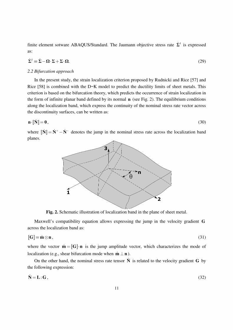
criterion is based on the bifurcation theory, which predicts the occurrence of strain localization in
the form of infinite planar band defined by its normal n (see Fig. 2). The equilibrium conditions
along the localization band, which express the continuity of the nominal stress rate vector across
the discontinuity surfaces, can be written as:
n N 0⋅ =ɺ� � , (30)
where N N N+ −= −ɺ ɺ ɺ� � denotes the jump in the nominal stress rate across the localization band
planes.
Fig. 2. Schematic illustration of localization band in the plane of sheet metal.
Maxwell’s compatibility equation allows expressing the jump in the velocity gradient G
across the localization band as:
G m n⊗= ɺ� � , (31)
where the vector m G n= ⋅ɺ � � is the jump amplitude vector, which characterizes the mode of
localization (e.g., shear bifurcation mode when m n⊥ɺ ).
On the other hand, the nominal stress rate tensor Nɺ is related to the velocity gradient G by
the following expression:
N L G= :ɺ , (32)
12
where L is the corresponding tangent modulus that needs to be determined. By combining Eqs.
(30-32), the critical condition, which corresponds to the loss of ellipticity for the boundary value
problem, can be expressed as the singularity of the acoustic tensor Q n L n= ⋅ ⋅ :
( ) ( )det det 0Q n L n= ⋅ ⋅ = . (33)
As for the sake of material objectivity, Jaumann stress rate has been used in the present work.
Within the framework of an updated Lagrangian approach, the expression of the nominal stress
rate tensor is given by:
( )trN Σ D Σ D Σ Ω Σ= + − ⋅ − ⋅ɺ ɺ . (34)
Finally, by combining the above equations, the complete expression of the tangent modulus
L is given by:
ep
1 2 3L C C C C= + − − , (35)
where 1C , 2C and 3C are fourth-order tensors, whose expressions are only function of the
Cauchy stress components. Their expressions are:
( )
( )
1i jkl ij kl
2ijkl jk il jl ik
3ijkl ik jl il jk
C ,
1C ,
2
1C ,
2
Σ δ
Σ δ Σ δ
Σ δ Σ δ
=
= +
= −
(36)
where ijδ is the kronecker symbol, which is equal to 1 when i j= , and to 0 otherwise.
It is worth noting that the present work is dedicated to the prediction of localized necking in
thin sheet metals. Although the constitutive equations presented in the previous section are
formulated in the fully three-dimensional framework, the Rice bifurcation criterion is derived in
this work in the framework of plane-stress conditions. To achieve this, the nominal stress rate
tensor, defined by Eq. (32), is rewritten within the framework of plane-stress theory as follows:
PSN L G , with , , , 1, 2αβ αβγδ γδ= α β γ δ =ɺ , (37)
where the expression of the plane-stress tangent modulus PSL is deduced from the three-
dimensional tangent modulus L using the following relationship:
33PS
33
3333
LL L L
L
γδ
αβγδ αβγδ αβ= − . (38)
Note that, within the plane-stress framework, the emergence of the localization band is
searched for in the plane of the sheet, with a variation of the band orientation angle θ (see Fig.
13
(2)) from 0° to 180°. Localized necking is said to occur when the minimum value, over all
possible band orientations, of the determinant of the acoustic tensor (see Eq. (33)) becomes zero.
The corresponding in-plane strains are considered as the critical strains at localization, which
will be used for the FLD plot.
3. Numerical implementation of the D−K model and validation
3.1 Time integration scheme and finite element implementation
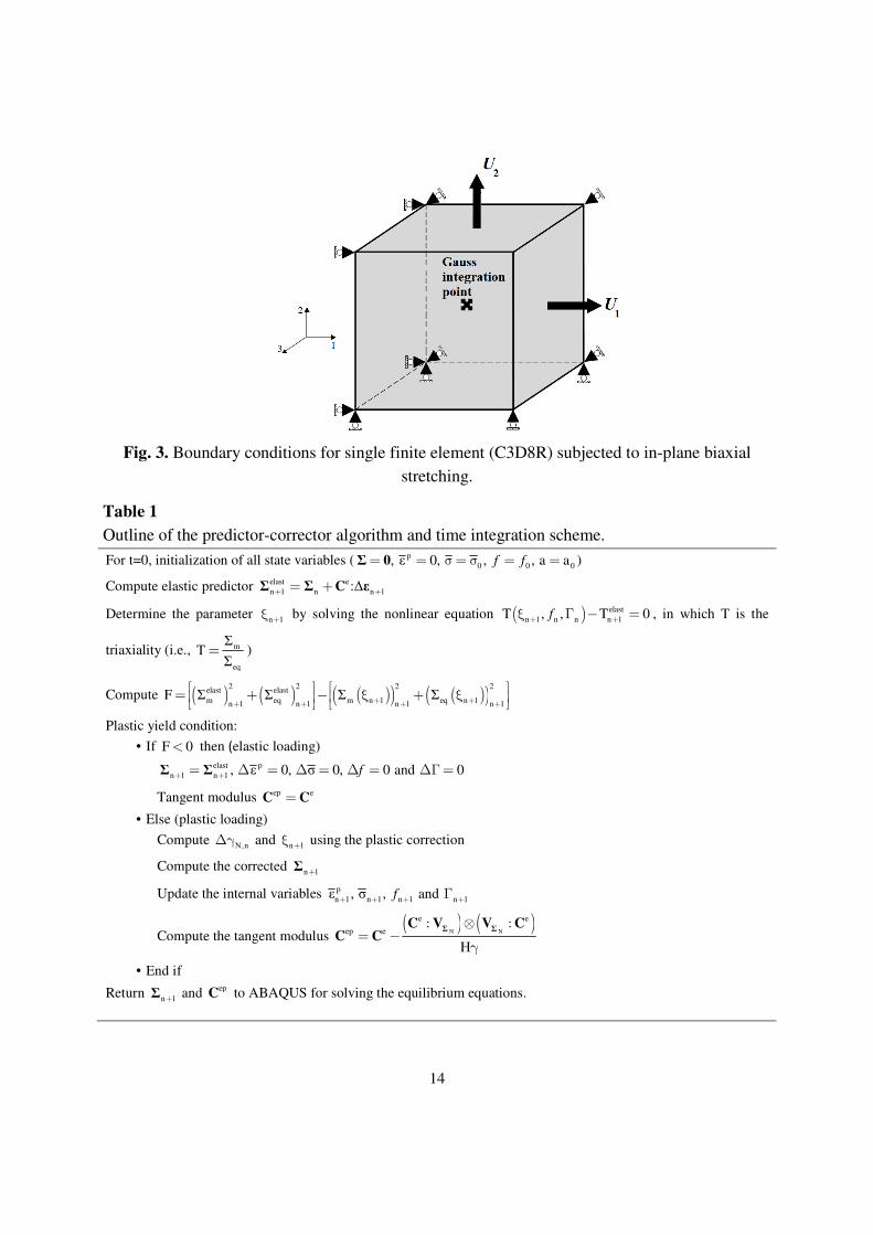
The constitutive equations described above have been implemented into the finite element
code ABAQUS/Standard in the framework of large strains and three-dimensional approach. In
order to reproduce a homogeneous strain state prior to localization, a single finite element with
one integration point (specifically, C3D8R solid element in ABAQUS) is used in the
simulations, which is subjected to various linear strain paths that are those typically applied to
sheet metals under in-plane biaxial stretching. The main motivation behind this choice of loading
configuration is to predict plastic instability that is inherent to the ‘material’ alone, with no
interference with structural (geometric) effects. The geometry of the single finite element along
with the applied boundary conditions are illustrated in Fig. 3. Directions 1 and 2 represent the
major and the minor directions, respectively. The linear strain paths are obtained by varying the
strain-path ratio from −0.5, for uniaxial tension, to 1 for balanced biaxial tension. For each
loading increment, the stress state is updated using a predictor-corrector approach, following the
numerical procedure proposed by Morin et al. [24]. The resulting numerical algorithm is detailed
in Table 1. As to the numerical implementation of the Rice bifurcation criterion, the condition of
loss of ellipticity, given by Eq. (33), is assessed by computing the determinant of the acoustic
tensor for each loading increment and each orientation for the localization band. The numerical
detection of the occurrence of localized necking is achieved when the minimum of the acoustic
tensor determinant, over all possible orientations for the normal n to the localization band,
becomes non-positive. This procedure is repeated for different strain-path ratios ranging from
uniaxial tension to balanced biaxial tension. Then, the corresponding in-plane critical strains are
plotted in terms of FLD.
14
Fig. 3. Boundary conditions for single finite element (C3D8R) subjected to in-plane biaxial
stretching.
Table 1
Outline of the predictor-corrector algorithm and time integration scheme.
For t=0, initialization of all state variables ( p
0 0 0, ε 0, , , a af fΣ 0= = σ= σ = = )
Compute elastic predictor elast e
n 1 n n 1:ΔΣ Σ C ε+ += +
Determine the parameter n 1+ξ by solving the nonlinear equation ( ) elast
n 1 n n n 1T , , T 0f+ +ξ Γ − = , in which T is the
triaxiality (i.e., m
eq
ΣT
Σ= )
Compute ( ) ( ) ( )( ) ( )( )2 2 2 2
elast elast
m eq m n 1 eq n 1n 1 n 1 n 1 n 1F Σ Σ Σ Σ+ ++ + + +
= + − ξ + ξ
Plastic yield condition:
• If F 0< then (elastic loading)
elast p
n 1 n 1 , ε 0, σ 0, 0 and 0fΣ Σ+ += ∆ = ∆ = ∆ = ∆Γ=
Tangent modulus ep eC C=
• Else (plastic loading)
Compute N,n∆γ and
n 1+ξ using the plastic correction
Compute the corrected n 1Σ +
Update the internal variables p
n 1 n 1 n 1 n 1ε , σ , andf+ + + +Γ
Compute the tangent modulus ( ) ( )
N N
e e
ep e
H
Σ ΣC V V C
C C: ⊗ :
= −γ
• End if
Return n 1Σ + and
epC to ABAQUS for solving the equilibrium equations.
15
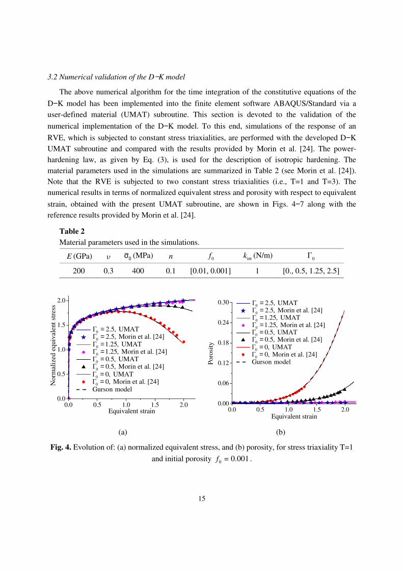
3.2 Numerical validation of the D−K model
The above numerical algorithm for the time integration of the constitutive equations of the
D−K model has been implemented into the finite element software ABAQUS/Standard via a
user-defined material (UMAT) subroutine. This section is devoted to the validation of the
numerical implementation of the D−K model. To this end, simulations of the response of an
RVE, which is subjected to constant stress triaxialities, are performed with the developed D−K
UMAT subroutine and compared with the results provided by Morin et al. [24]. The power-
hardening law, as given by Eq. (3), is used for the description of isotropic hardening. The
material parameters used in the simulations are summarized in Table 2 (see Morin et al. [24]).
Note that the RVE is subjected to two constant stress triaxialities (i.e., T=1 and T=3). The
numerical results in terms of normalized equivalent stress and porosity with respect to equivalent
strain, obtained with the present UMAT subroutine, are shown in Figs. 4−7 along with the
reference results provided by Morin et al. [24].
Table 2
Material parameters used in the simulations.
E (GPa) ν σ0
(MPa) n 0f
intk (N/m) 0Γ
200 0.3 400 0.1 [0.01, 0.001] 1 [0., 0.5, 1.25, 2.5]
0.0 0.5 1.0 1.5 2.00.0
0.5
1.0
1.5
2.0
Norm
aliz
ed e
quiv
ale
nt
stre
ss
Gurson model
Equivalent strain
0Γ 0, Morin et al. [24]=0Γ 0, UMAT=
0Γ 0.5, UMAT=0Γ 0.5, Morin et al. [24]=
0Γ 1.25, Morin et al. [24]=0Γ 1.25, UMAT=0Γ 2.5, Morin et al. [24]=0Γ 2.5, UMAT=
0.0 0.5 1.0 1.5 2.00.00
0.06
0.12
0.18
0.24
0.30
Poro
sity
Equivalent strain
Gurson model0Γ 0, Morin et al. [24]=
0Γ 0, UMAT=
0Γ 0.5, UMAT=0Γ 0.5, Morin et al. [24]=
0Γ 1.25, Morin et al. [24]=
0Γ 1.25, UMAT=
0Γ 2.5, Morin et al. [24]=
0Γ 2.5, UMAT=
(a) (b)
Fig. 4. Evolution of: (a) normalized equivalent stress, and (b) porosity, for stress triaxiality T=1
and initial porosity 0
= 0.001f .
16
0.0 0.5 1.0 1.50.0
0.5
1.0
1.5
2.0
Norm
aliz
ed e
quiv
ale
nt
stre
ss
Equivalent strain
Gurson model0Γ 0, Morin et al. [24]=0Γ 0, UMAT=
0Γ 0.5, UMAT=0Γ 0.5, Morin et al. [24]=
0Γ 1.25, Morin et al. [24]=0Γ 1.25, UMAT=0Γ 2.5, Morin et al. [24]=0Γ 2.5, UMAT=
0.0 0.5 1.0 1.5
0.0
0.1
0.2
0.3
0.4
Poro
sity
Equivalent strain
Gurson model0Γ 0, Morin et al. [24]=
0Γ 0, UMAT=
0Γ 0.5, UMAT=0Γ 0.5, Morin et al. [24]=
0Γ 1.25, Morin et al. [24]=0Γ 1.25, UMAT=0Γ 2.5, Morin et al. [24]=
0Γ 2.5, UMAT=
(a) (b)
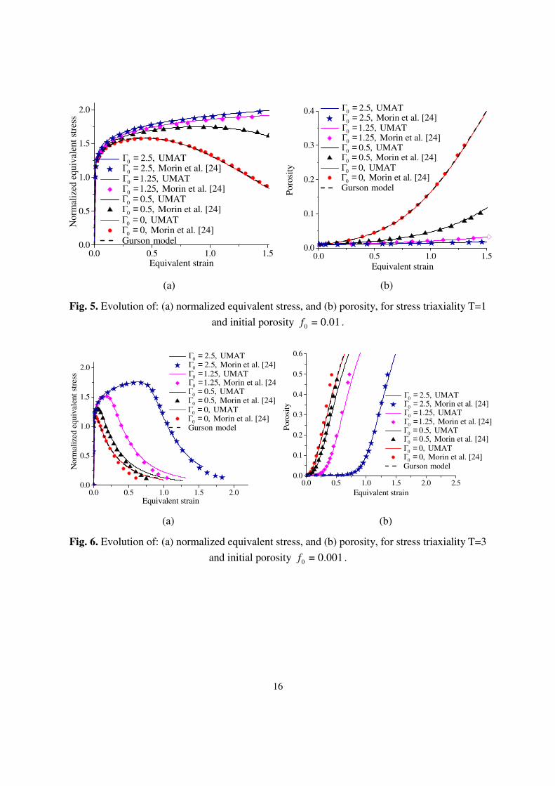
Fig. 5. Evolution of: (a) normalized equivalent stress, and (b) porosity, for stress triaxiality T=1
and initial porosity 0
= 0.01f .
0.0 0.5 1.0 1.5 2.00.0
0.5
1.0
1.5
2.0
No
rmal
ized
equ
ival
ent
stre
ss
Equivalent strain
Gurson model0Γ 0, Morin et al. [24]=0Γ 0, UMAT=
0Γ 0.5, UMAT=
0Γ 0.5, Morin et al. [24]=
0Γ 1.25, Morin et al. [24]=0Γ 1.25, UMAT=0Γ 2.5, Morin et al. [24]=0Γ 2.5, UMAT=
0.0 0.5 1.0 1.5 2.0 2.50.0
0.1
0.2
0.3
0.4
0.5
0.6
Po
rosi
ty
Equivalent strain
Gurson model0Γ 0, Morin et al. [24]=0Γ 0, UMAT=
0Γ 0.5, UMAT=0Γ 0.5, Morin et al. [24]=
0Γ 1.25, Morin et al. [24]=0Γ 1.25, UMAT=0Γ 2.5, Morin et al. [24]=0Γ 2.5, UMAT=
(a) (b)
Fig. 6. Evolution of: (a) normalized equivalent stress, and (b) porosity, for stress triaxiality T=3
and initial porosity 0
= 0.001f .
17
0.0 0.5 1.0 1.5 2.0 2.50.0
0.5
1.0
1.5
2.0
Norm
aliz
ed e
qu
ival
ent
stre
ss
Equivalent strain
Gurson model0Γ 0, Morin et al. [24]=0Γ 0, UMAT=
0Γ 0.5, UMAT=0Γ 0.5, Morin et al. [24]=
0Γ 1.25, Morin et al. [24]=0Γ 1.25, UMAT=0Γ 2.5, Morin et al. [24]=0Γ 2.5, UMAT=
0.0 0.5 1.0 1.5 2.0 2.50.0
0.1
0.2
0.3
0.4
0.5
0.6
Po
rosi
ty
Equivalent strain
Gurson model0Γ 0, Morin et al. [24]=0Γ 0, UMAT=
0Γ 0.5, UMAT=0Γ 0.5, Morin et al. [24]=
0Γ 1.25, Morin et al. [24]=0Γ 1.25, UMAT=0Γ 2.5, Morin et al. [24]=0Γ 2.5, UMAT=
(a) (b)
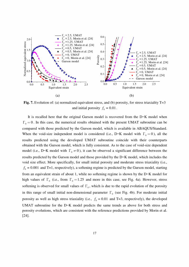
Fig. 7. Evolution of: (a) normalized equivalent stress, and (b) porosity, for stress triaxiality T=3
and initial porosity 0
= 0.01f .
It is recalled here that the original Gurson model is recovered from the D−K model when
0 0Γ = . In this case, the numerical results obtained with the present UMAT subroutine can be
compared with those predicted by the Gurson model, which is available in ABAQUS/Standard.
When the void-size independent model is considered (i.e., D−K model with 0 0Γ = ), all the
results predicted using the developed UMAT subroutine coincide with their counterparts
obtained with the Gurson model, which is fully consistent. As to the case of void-size dependent
model (i.e., D−K model with 0 0Γ ≠ ), it can be observed a significant difference between the
results predicted by the Gurson model and those provided by the D−K model, which includes the
void size effect. More specifically, for small initial porosity and moderate stress triaxiality (i.e.,
0= 0.001f and T=1, respectively), a softening regime is predicted by the Gurson model, starting
from an equivalent strain of about 1, while no softening regime is shown by the D−K model for
high values of 0Γ (i.e., from 0 1.25Γ = and more in this case, see Fig. 4a). However, stress
softening is observed for small values of 0Γ , which is due to the rapid evolution of the porosity
in this range of small initial non-dimensional parameter 0Γ (see Fig. 4b). For moderate initial
porosity as well as high stress triaxiality (i.e., 0
= 0.01f and T=3, respectively), the developed
UMAT subroutine for the D−K model predicts the same trends as above for both stress and
porosity evolutions, which are consistent with the reference predictions provided by Morin et al.
[24].
18
4. Prediction of FLDs with the D−K model and bifurcation analysis
In this section, the resulting coupling between the D−K model and the Rice bifurcation
criterion is applied for the prediction of FLDs for Al5754 aluminum material. The associated
material parameters used in the simulations are taken from Mansouri et al. [64], as reported in
Table 3. The additional parameter 0Γ , which incorporates the void size effect is varied here to
analyze its effect on the prediction of localized necking.
Table 3
Material parameters for the Al5754 aluminum material.
Elastic properties Swift’s hardening parameters Initial porosity
E (GPa) ν K ε0 n 0
f
70 0.33 309.1 0.00173 0.177 0.001
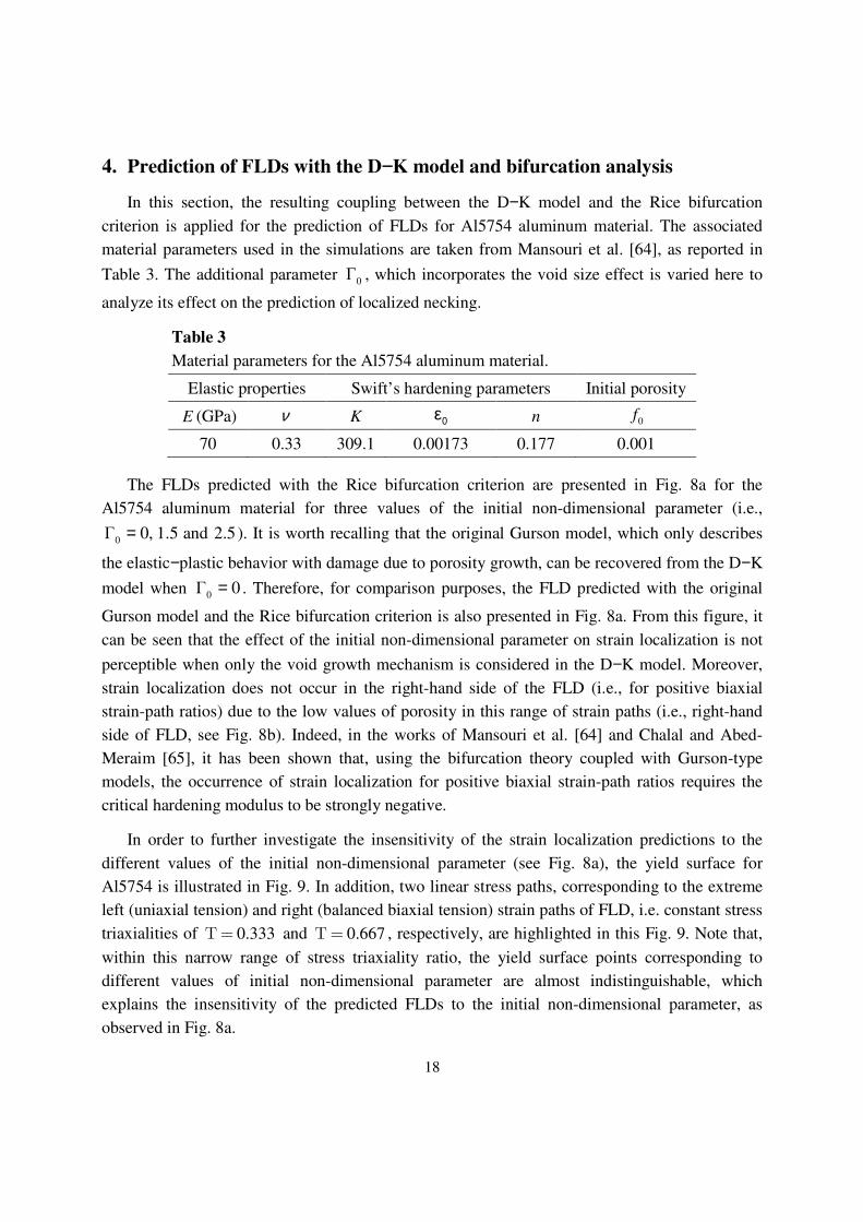
The FLDs predicted with the Rice bifurcation criterion are presented in Fig. 8a for the
Al5754 aluminum material for three values of the initial non-dimensional parameter (i.e.,
0Γ 0, 1.5 and 2.5= ). It is worth recalling that the original Gurson model, which only describes
the elastic−plastic behavior with damage due to porosity growth, can be recovered from the D−K
model when 0Γ 0= . Therefore, for comparison purposes, the FLD predicted with the original
Gurson model and the Rice bifurcation criterion is also presented in Fig. 8a. From this figure, it
can be seen that the effect of the initial non-dimensional parameter on strain localization is not
perceptible when only the void growth mechanism is considered in the D−K model. Moreover,
strain localization does not occur in the right-hand side of the FLD (i.e., for positive biaxial
strain-path ratios) due to the low values of porosity in this range of strain paths (i.e., right-hand
side of FLD, see Fig. 8b). Indeed, in the works of Mansouri et al. [64] and Chalal and Abed-
Meraim [65], it has been shown that, using the bifurcation theory coupled with Gurson-type
models, the occurrence of strain localization for positive biaxial strain-path ratios requires the
critical hardening modulus to be strongly negative.
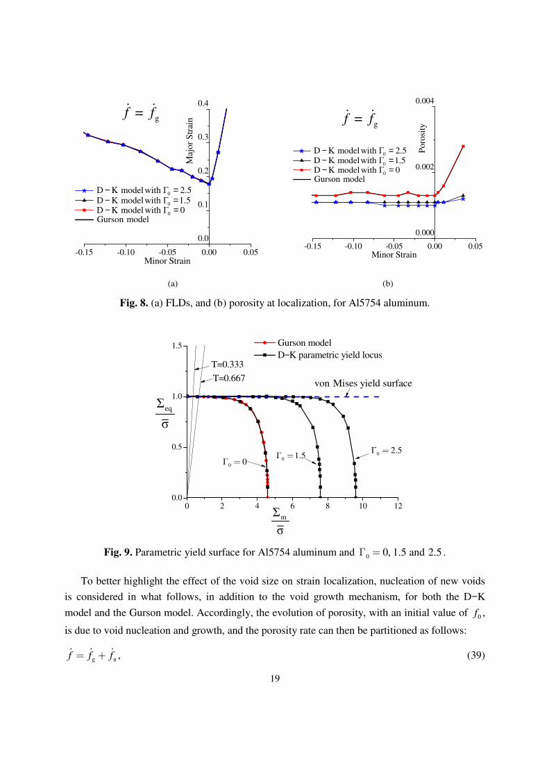
In order to further investigate the insensitivity of the strain localization predictions to the
different values of the initial non-dimensional parameter (see Fig. 8a), the yield surface for
Al5754 is illustrated in Fig. 9. In addition, two linear stress paths, corresponding to the extreme
left (uniaxial tension) and right (balanced biaxial tension) strain paths of FLD, i.e. constant stress
triaxialities of 0.333Τ= and 0.667Τ= , respectively, are highlighted in this Fig. 9. Note that,
within this narrow range of stress triaxiality ratio, the yield surface points corresponding to
different values of initial non-dimensional parameter are almost indistinguishable, which
explains the insensitivity of the predicted FLDs to the initial non-dimensional parameter, as
observed in Fig. 8a.
19
-0.15 -0.10 -0.05 0.00 0.05
0.0
0.1
0.2
0.3
0.4
Gurson model
0D K modelwith Γ 2.5− =0D K modelwith Γ 1.5− =
Maj
or
Str
ain
Minor Strain
0D K model with Γ 0− =
gf = fɺ ɺ
-0.15 -0.10 -0.05 0.00 0.05
0.000
0.002
0.004
gf = fɺ ɺ
Poro
sity
Minor Strain
Gurson model
0D K model with Γ 2.5− =
0D K modelwith Γ 1.5− =
0D K model with Γ 0− =
(a) (b)
Fig. 8. (a) FLDs, and (b) porosity at localization, for Al5754 aluminum.
0 2 4 6 8 10 120.0
0.5
1.0
1.5
von Mises yield surfaceT=0.667
0Γ 2.5=0Γ 1.5=
eqΣ
σ
T=0.333
0Γ 0=
mΣ
σ
Gurson model
D−K parametric yield locus
Fig. 9. Parametric yield surface for Al5754 aluminum and 0 0, 1.5 and 2.5Γ = .
To better highlight the effect of the void size on strain localization, nucleation of new voids
is considered in what follows, in addition to the void growth mechanism, for both the D−K
model and the Gurson model. Accordingly, the evolution of porosity, with an initial value of 0f ,
is due to void nucleation and growth, and the porosity rate can then be partitioned as follows:
g n ,f f f= +ɺ ɺ ɺ (39)
20
where nfɺ represents the contribution to the porosity rate from nucleation. The latter is
considered to be strain-controlled following the normal distribution relationship proposed by
Chu and Needleman [67]:
2p
pN Nn
NN
ε ε1exp ε ,
2 ss 2
ff
− = − π
ɺ ɺ (40)
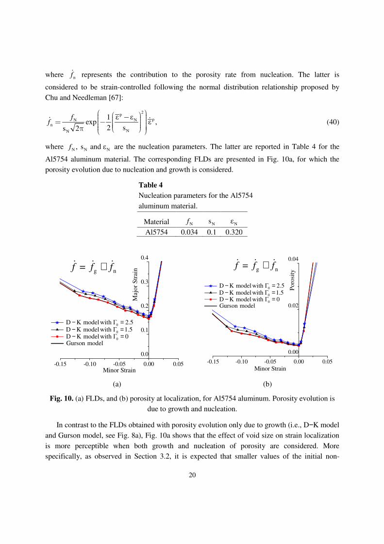
where N N N, s and εf are the nucleation parameters. The latter are reported in Table 4 for the
Al5754 aluminum material. The corresponding FLDs are presented in Fig. 10a, for which the
porosity evolution due to nucleation and growth is considered.
Table 4
Nucleation parameters for the Al5754
aluminum material.
Material Nf Ns Nε
Al5754 0.034 0.1 0.320
-0.15 -0.10 -0.05 0.00 0.05
0.0
0.1
0.2
0.3
0.4
g nf = f f+ɺ ɺ ɺ
Maj
or
Str
ain
Minor Strain
Gurson model
0D K model with Γ 2.5− =
0D K model with Γ 1.5− =
0D K model with Γ 0− =
-0.15 -0.10 -0.05 0.00 0.05
0.00
0.02
0.04
Po
rosi
ty
Minor Strain
g nf = f f+ɺ ɺ ɺ
Gurson model
0D K model with Γ 2.5− =
0D K model with Γ 1.5− =
0D K model with Γ 0− =
(a) (b)
Fig. 10. (a) FLDs, and (b) porosity at localization, for Al5754 aluminum. Porosity evolution is
due to growth and nucleation.
In contrast to the FLDs obtained with porosity evolution only due to growth (i.e., D−K model
and Gurson model, see Fig. 8a), Fig. 10a shows that the effect of void size on strain localization
is more perceptible when both growth and nucleation of porosity are considered. More
specifically, as observed in Section 3.2, it is expected that smaller values of the initial non-
21
dimensional parameter induce rapid softening (see the stress−strain curves in Figs. 4 and 5),
thereby promoting early plastic flow localization. This expectation is also confirmed by Fig. 10a,
which shows that the predicted FLDs are lowered as initial non-dimensional parameter 0Γ
decreases. This trend is confirmed by Fig. 10b, which also shows the effect of the initial non-
dimensional parameter on the values of porosity at localization. Note that when 0Γ 0= , the FLD
predicted by the D−K model coincides with that of the Gurson model, which is also consistent
with the theoretical expectation for this particular case (i.e., the Gurson model is recovered from
the D−K model when 0Γ 0= ).
In addition to growth and nucleation of voids during plastic deformation in ductile materials,
coalescence of voids can also be introduced to model the rapid decay of the material stress
carrying capacity. Tvergaard and Needleman [68] have modified the original Gurson model to
account for the complete kinetics of voids within the material (i.e., nucleation, growth and
coalescence), which corresponds to the well-known Gurson–Tvergaard–Needleman (GTN)
model. Using the GTN model, the actual void volume fraction f in the expression of the yield
surface is replaced by the effective porosity *f , which accounts for the void coalescence
mechanism as follows:
*
cr GTN cr( ),f f δ f f= + − (41)
where crf is the critical porosity, which marks the onset of the coalescence regime, while GTNδ is
the accelerating factor that governs the rapid decay of stress carrying capacity at the onset of
coalescence. Note that when crf f≤ (i.e., only growth and nucleation of voids are considered),
the accelerating factor GTNδ is set to 1, while GTN 1δ > in the case of coalescence (i.e., crf f> ).
This approach, which considers the coalescence of voids beyond a critical porosity, is also used
for the D−K model in what follows.
The parameters associated with the coalescence regime for the Al5754 aluminum material
are reported in Table 5, while the elastic−plastic and nucleation parameters are kept the same as
those used in Tables 3 and 4. The corresponding FLDs obtained with the developed approach are
presented in Fig. 11a. As discussed above, coalescence causes sudden loss of the stress carrying
capacity and, therefore, the hardening modulus becomes strongly negative. It has been shown in
Mansouri et al. [64] that the prediction of strain localization using the Rice bifurcation criterion
requires strongly negative hardening modulus in the right-hand side of the FLD (i.e., for biaxial
stretching loading paths), which can be reached by considering the coalescence mechanism.
Consequently, it can be observed in Fig. 11a that more localization points are obtained in the
right-hand side of the FLD, as compared to the FLDs in Figs. 8a and 10a, thanks to the
consideration of the void coalescence mechanism. Note that the experimental FLD, which is
taken from Brunet et al. [69], is also shown in Fig. 11a for qualitative comparison.
22
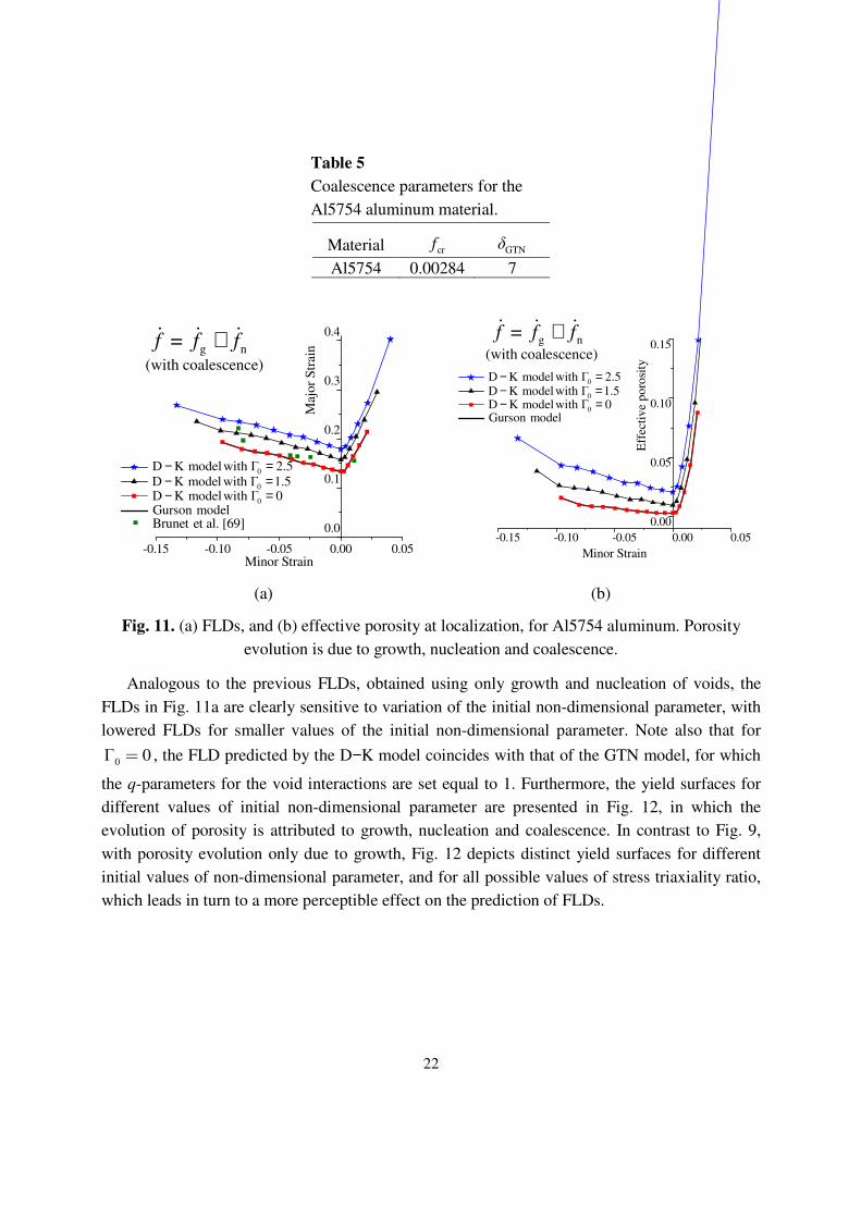
Table 5
Coalescence parameters for the
Al5754 aluminum material.
Material crf GTNδ
Al5754 0.00284 7
-0.15 -0.10 -0.05 0.00 0.05
0.0
0.1
0.2
0.3
0.4
Brunet et al. [69]
Maj
or
Str
ain
Minor Strain
Gurson model
0D K modelwith Γ 2.5− =0D K model with Γ 1.5− =
0D K modelwith Γ 0− =
(with coalescence)g n
+ɺ ɺ ɺf = f f
-0.15 -0.10 -0.05 0.00 0.05
0.00
0.05
0.10
0.15(with coalescence)
Eff
ecti
ve
po
rosi
ty
Minor Strain
g n +ɺ ɺ ɺf = f f
Gurson model
0D K model with Γ 2.5− =0
D K model with Γ 1.5− =
0D K modelwith Γ 0− =
(a) (b)
Fig. 11. (a) FLDs, and (b) effective porosity at localization, for Al5754 aluminum. Porosity
evolution is due to growth, nucleation and coalescence.
Analogous to the previous FLDs, obtained using only growth and nucleation of voids, the
FLDs in Fig. 11a are clearly sensitive to variation of the initial non-dimensional parameter, with
lowered FLDs for smaller values of the initial non-dimensional parameter. Note also that for
0Γ 0= , the FLD predicted by the D−K model coincides with that of the GTN model, for which
the q-parameters for the void interactions are set equal to 1. Furthermore, the yield surfaces for
different values of initial non-dimensional parameter are presented in Fig. 12, in which the
evolution of porosity is attributed to growth, nucleation and coalescence. In contrast to Fig. 9,
with porosity evolution only due to growth, Fig. 12 depicts distinct yield surfaces for different
initial values of non-dimensional parameter, and for all possible values of stress triaxiality ratio,
which leads in turn to a more perceptible effect on the prediction of FLDs.
23
0 1 2 30.0
0.5
1.0von Mises yield surfaceT
=0.6
67
0Γ 2.5=
0Γ 1.5=
eqΣ
σ
T=
0.3
33
0Γ 0=
mΣ
σ
Gurson model
D−K parametric yield locus
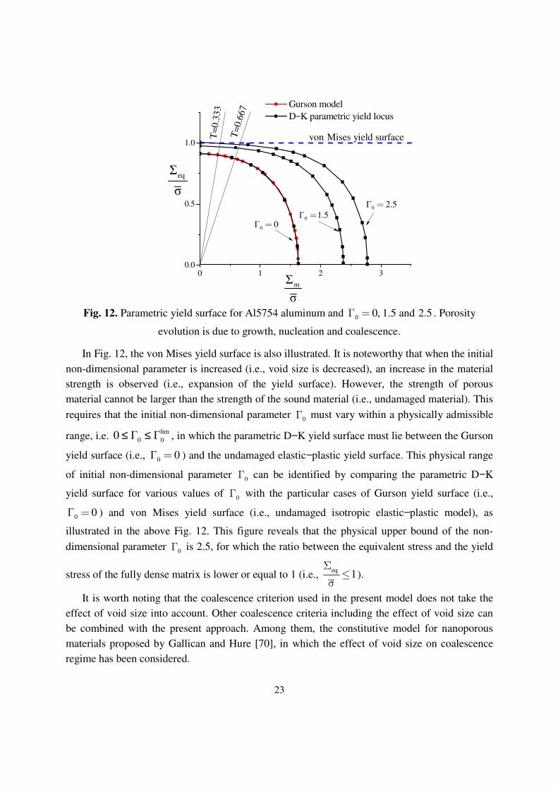
Fig. 12. Parametric yield surface for Al5754 aluminum and 0 0, 1.5 and 2.5Γ = . Porosity
evolution is due to growth, nucleation and coalescence.
In Fig. 12, the von Mises yield surface is also illustrated. It is noteworthy that when the initial
non-dimensional parameter is increased (i.e., void size is decreased), an increase in the material
strength is observed (i.e., expansion of the yield surface). However, the strength of porous
material cannot be larger than the strength of the sound material (i.e., undamaged material). This
requires that the initial non-dimensional parameter 0
Γ must vary within a physically admissible
range, i.e. lim
0 00 Γ Γ≤ ≤ , in which the parametric D−K yield surface must lie between the Gurson
yield surface (i.e., 0Γ 0= ) and the undamaged elastic−plastic yield surface. This physical range
of initial non-dimensional parameter 0
Γ can be identified by comparing the parametric D−K
yield surface for various values of 0
Γ with the particular cases of Gurson yield surface (i.e.,
0Γ 0= ) and von Mises yield surface (i.e., undamaged isotropic elastic−plastic model), as
illustrated in the above Fig. 12. This figure reveals that the physical upper bound of the non-
dimensional parameter 0
Γ is 2.5, for which the ratio between the equivalent stress and the yield
stress of the fully dense matrix is lower or equal to 1 (i.e., eq
1Σ
≤σ
).
It is worth noting that the coalescence criterion used in the present model does not take the
effect of void size into account. Other coalescence criteria including the effect of void size can
be combined with the present approach. Among them, the constitutive model for nanoporous
materials proposed by Gallican and Hure [70], in which the effect of void size on coalescence
regime has been considered.
24
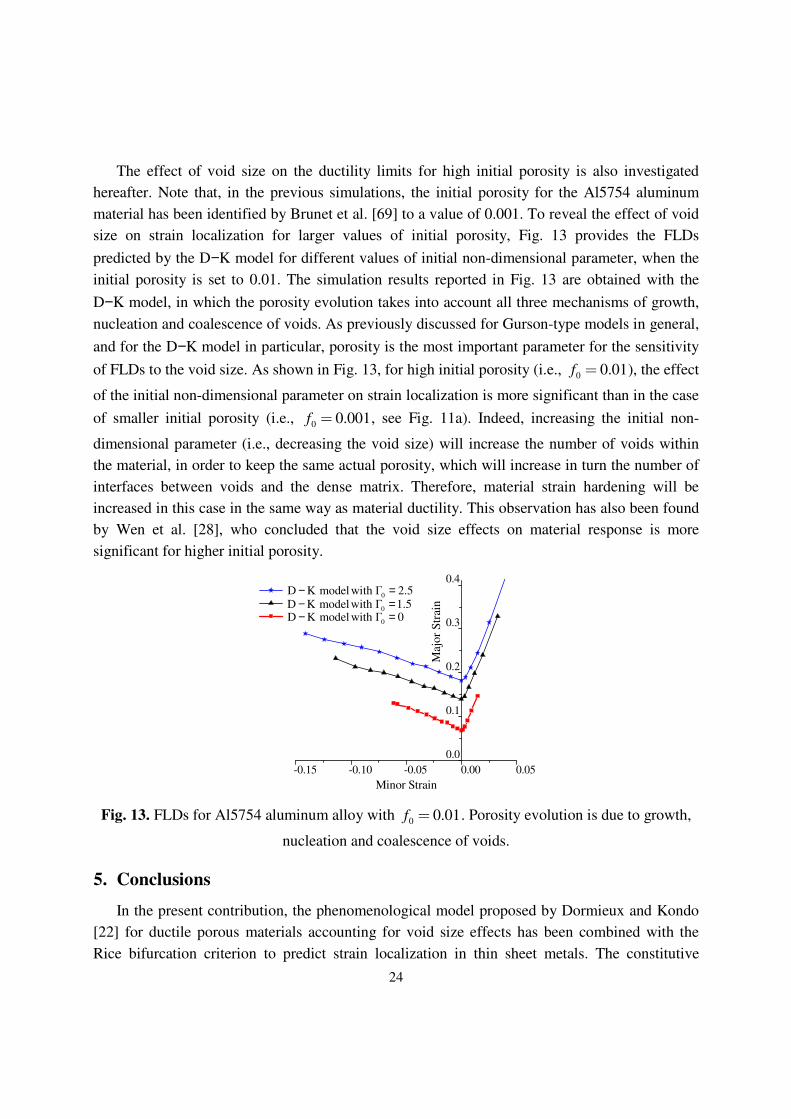
The effect of void size on the ductility limits for high initial porosity is also investigated
hereafter. Note that, in the previous simulations, the initial porosity for the Al5754 aluminum
material has been identified by Brunet et al. [69] to a value of 0.001. To reveal the effect of void
size on strain localization for larger values of initial porosity, Fig. 13 provides the FLDs
predicted by the D−K model for different values of initial non-dimensional parameter, when the
initial porosity is set to 0.01. The simulation results reported in Fig. 13 are obtained with the
D−K model, in which the porosity evolution takes into account all three mechanisms of growth,
nucleation and coalescence of voids. As previously discussed for Gurson-type models in general,
and for the D−K model in particular, porosity is the most important parameter for the sensitivity
of FLDs to the void size. As shown in Fig. 13, for high initial porosity (i.e., 0 0.01f = ), the effect
of the initial non-dimensional parameter on strain localization is more significant than in the case
of smaller initial porosity (i.e., 0 0.001f = , see Fig. 11a). Indeed, increasing the initial non-
dimensional parameter (i.e., decreasing the void size) will increase the number of voids within
the material, in order to keep the same actual porosity, which will increase in turn the number of
interfaces between voids and the dense matrix. Therefore, material strain hardening will be
increased in this case in the same way as material ductility. This observation has also been found
by Wen et al. [28], who concluded that the void size effects on material response is more
significant for higher initial porosity.
-0.15 -0.10 -0.05 0.00 0.05
0.0
0.1
0.2
0.3
0.4
Maj
or
Str
ain
Minor Strain
0D K model with Γ 2.5− =
0D K modelwith Γ 1.5− =
0D K model with Γ 0− =
Fig. 13. FLDs for Al5754 aluminum alloy with 0 0.01f = . Porosity evolution is due to growth,
nucleation and coalescence of voids.
5. Conclusions
In the present contribution, the phenomenological model proposed by Dormieux and Kondo
[22] for ductile porous materials accounting for void size effects has been combined with the
Rice bifurcation criterion to predict strain localization in thin sheet metals. The constitutive
25
equations have been implemented together with the Rice bifurcation criterion into the finite
element code ABAQUS/Standard within the framework of large strains and fully three-
dimensional approach. However, the localization bifurcation criterion has been reformulated
within the plane-stress framework, as classically done for the prediction of localized necking in
thin sheet metals. Linear in-plane biaxial stretching loading paths have been applied for the
prediction of forming limit diagrams for the Al5754 aluminum material.
Recall that the Dormieux and Kondo [22] model, which is an extension of the original
Gurson model, has been developed by performing a limit analysis for a spherical void inside a
spherical RVE, and by considering a membrane with surface stresses around the void. The
resulting yield function depends on the void size through a non-dimensional parameter.
Considering at first only the porosity evolution due to void growth, the FLDs predicted with the
present approach show no sensitivity to the void size, due to the fact that the porosity at
localization remains very small. However, when successively nucleation and coalescence are
considered in the evolution of porosity, FLDs exhibit more sensitivity to the void size. More
specifically, it is found that the ductility limits are lowered as the initial non-dimensional
parameter is decreased (i.e., when the void size is increased). In other words, decreasing the void
size has a beneficial effect on formability. These findings are consistent with what has been
reported in the literature regarding the void size effects on material response. Nonetheless, there
is an upper bound for the initial non-dimensional parameter 0Γ (i.e., lower bound for the void
size), which is physically admissible. This upper bound, which depends on the material
parameters, is identified so that the parametric D−K yield surface must lie between the Gurson
yield surface and the undamaged elastic−plastic yield surface (i.e., sound material with no void).
Moreover, it is found that the FLD predicted using the D−K model with an initial non-
dimensional parameter 0Γ 0= coincides with that obtained with the Gurson model, which is
also consistent with the material response for this particular case. Finally, the investigation of the
combined effect of void size and initial porosity shows that smaller void sizes lead to an increase
in the ductility limits, and this trend becomes more significant for high initial porosity, due to the
increase of void-matrix interface strength within the material.
References
1. Keeler SP, Backofen WA. Plastic instability and fracture in sheets stretched over rigid
punches. ASM Transactions Quarterly 1963;56(11):25-48.
2. Goodwin GM. Application of strain analysis to sheet metal forming problems in the press
shop. SAE Transactions 1968;380-87.
3. Kachanov LM. On creep rupture time. Izv. Acad. Nauk SSSR, Otd. Techn. Nauk 1958;8:26-
31.
26
4. Rabotnov YN. Creep problems in structural members. North-Holland Publishing Company
1969.
5. Lemaitre J. A Course on Damage Mechanics. Springer Science & Business Media 1992.
6. Maire JF, Chaboche JL. A new formulation of continuum damage mechanics (CDM) for
composite materials. Aerospace Science and Technology 1997;1(4):247-57.
7. Hambli R. Comparison between Lemaitre and Gurson damage models in crack growth
simulation during blanking process. International Journal of Mechanical Sciences
2001;43(12):2769-90.
8. Brünig M. Numerical analysis and elastic–plastic deformation behavior of anisotropically
damaged solids. International Journal of Plasticity 2002;18(9):1237-70.
9. Menzel A, Ekh M, Runesson K, Steinmann P. A framework for multiplicative
elastoplasticity with kinematic hardening coupled to anisotropic damage. International
Journal of Plasticity 2005;21(3):397-434.
10. Besson J, Cailletaud G, Chaboche JL, Forest S. Non-linear mechanics of materials. Springer
Science & Business Media 2009;167
11. Bouchard PO, Bourgeon L, Fayolle S, Mocellin K. An enhanced Lemaitre model
formulation for materials processing damage computation. International Journal of Material
Forming 2011;4(3):299-315.
12. Voyiadjis G. Advances in damage mechanics: metals and metal matrix composites. Elsevier
2012.
13. Doghri I. Mechanics of deformable solids: linear, nonlinear, analytical and computational
aspects. Springer Science & Business Media 2013.
14. Lian J, Feng Y, Münstermann S. A modified Lemaitre damage model phenomenologically
accounting for the Lode angle effect on ductile fracture. Procedia materials science
2014;3:1841-47.
15. Gurson AL. Continuum theory of ductile rupture by void nucleation and growth: Part I—
Yield criteria and flow rules for porous ductile media. Journal of Engineering Materials and
Technology 1977;99(1):2-15.
16. Gologanu M, Leblond JB, Devaux J. Approximate models for ductile metals containing
non-spherical voids—case of axisymmetric prolate ellipsoidal cavities. Journal of the
Mechanics and Physics of Solids 1993;41(11):1723-54.
17. Gologanu M, Leblond JB, Devaux J. Approximate models for ductile metals containing
nonspherical voids—case of axisymmetric oblate ellipsoidal cavities. Journal of Engineering
Materials and Technology 1994;116(3):290-97.
18. Madou K, Leblond JB. A Gurson-type criterion for porous ductile solids containing
arbitrary ellipsoidal voids—I: Limit-analysis of some representative cell. Journal of the
Mechanics and Physics of Solids 2012;60(5):1020-36.
27
19. Madou K, Leblond JB. A Gurson-type criterion for porous ductile solids containing
arbitrary ellipsoidal voids—II: Determination of yield criterion parameters. Journal of the
Mechanics and Physics of Solids 2012;60(5):1037-58.
20. Madou K, Leblond JB. Numerical studies of porous ductile materials containing arbitrary
ellipsoidal voids–I: Yield surfaces of representative cells. European Journal of Mechanics-
A/Solids 2013;42:480-89.
21. Madou K, Leblond JB, Morin L. Numerical studies of porous ductile materials containing
arbitrary ellipsoidal voids–II: Evolution of the length and orientation of the void axes.
European Journal of Mechanics-A/Solids 2013;42:490-507.
22. Dormieux L, Kondo D. An extension of Gurson model incorporating interface stresses
effects. International Journal of Engineering Science 2010;48(6):575-81.
23. Monchiet V, Bonnet G. A Gurson-type model accounting for void size effects. International
Journal of Solids and Structures 2013;50(2):320-27.
24. Morin L, Kondo D, Leblond JB. Numerical assessment, implementation and application of
an extended Gurson model accounting for void size effects. European Journal of Mechanics-
A/Solids 2015;51:183-92.
25. Lacroix R, Leblond JB, Perrin G. Numerical study and theoretical modelling of void growth
in porous ductile materials subjected to cyclic loadings. European Journal of Mechanics-
A/Solids 2016;55:100-09.
26. Morin L, Michel JC, Leblond JB. A Gurson-type layer model for ductile porous solids with
isotropic and kinematic hardening. International Journal of Solids and Structures
2017;118:167-78.
27. Hutchinson JW. Plasticity at the micron scale. International Journal of Solids and Structures
2000;37(1-2):225-38.
28. Wen J, Huang Y, Hwang KC, Liu C, Li M. The modified Gurson model accounting for the
void size effect. International Journal of Plasticity 2005;21(2):381-95.
29. Fleck NA, Muller GM, Ashby MF, Hutchinson JW. Strain gradient plasticity: theory and
experiment. Acta Metallurgica et Materialia 1994;42(2):475-87.
30. Schlu N, Grimpe F, Bleck W, Dahl W. Modelling of the damage in ductile steels.
Computational Materials Science 1996;7(1-2):27-33.
31. Begley MR, Hutchinson JW. The mechanics of size-dependent indentation. Journal of the
Mechanics and Physics of Solids 1998;46(10):2049-68.
32. Nix WD, Gao H. Indentation size effects in crystalline materials: a law for strain gradient
plasticity. Journal of the Mechanics and Physics of Solids 1998;46(3):411-25.
33. Stölken JS, Evans AG. A microbend test method for measuring the plasticity length scale.
Acta Materialia 1998;46(14):5109-15.
34. Kawasaki M, Xu C, Langdon TG. An investigation of cavity growth in a superplastic
aluminum alloy processed by ECAP. Acta Materialia 2005;53(20):5353-64.
28
35. Khraishi TA, Khaleel MA, Zbib HM. A parametric-experimental study of void growth in
superplastic deformation. International Journal of Plasticity 2001;17(3):297-315.
36. Fu MW, Chan WL. Geometry and grain size effects on the fracture behavior of sheet metal
in micro-scale plastic deformation. Materials & Design 2011;32(10):4738-46.
37. Chentouf SM, Belhadj T, Bombardier N, Brodusch N, Gauvin R, Jahazi M. Influence of
predeformation on microstructure evolution of superplastically formed Al 5083 alloy. The
International Journal of Advanced Manufacturing Technology 2017;88(9-12):2929-37.
38. Li S, Jin S, Huang Z. Cavity Behavior of Fine-Grained 5A70 Aluminum Alloy during
Superplastic Formation. Metals 2018;8(12):1065.
39. Liu B, Qiu X, Huang Y, Hwang KC, Li M, Liu C. The size effect on void growth in ductile
materials. Journal of the Mechanics and Physics of Solids. 2003;51(7):1171-87.
40. Brach S, Dormieux L, Kondo D, Vairo G. A computational insight into void-size effects on
strength properties of nanoporous materials. Mechanics of Materials 2016;101:102-17.
41. Biener J, Hodge AM, Hamza AV, Hsiung LM, Satcher Jr JH. Nanoporous Au: A high yield
strength material. Journal of Applied Physics 2005;97(2):024301.
42. Biener J, Hodge AM, Hayes JR, Volkert CA, Zepeda-Ruiz LA, Hamza AV, Abraham FF.
Size effects on the mechanical behavior of nanoporous Au. Nano Letters 2006;6(10):2379-
82.
43. Hakamada M, Mabuchi M. Mechanical strength of nanoporous gold fabricated by
dealloying. Scripta Materialia 2007;56(11):1003-06.
44. Mi C, Buttry DA, Sharma P, Kouris DA. Atomistic insights into dislocation-based
mechanisms of void growth and coalescence. Journal of the Mechanics and Physics of
Solids 2011;59(9):1858-71.
45. Xu ZT, Peng LF, Fu MW, Lai XM. Size effect affected formability of sheet metals in
micro/meso scale plastic deformation: experiment and modeling. International Journal of
Plasticity 2015;68:34-54.
46. Xu ZT, Peng LF, Lai XM, Fu MW. Geometry and grain size effects on the forming limit of
sheet metals in micro-scaled plastic deformation. Materials Science and Engineering: A
2014;611:345-53.
47. Xu Z, Peng L, Yi P, Lai X. An investigation on the formability of sheet metals in the
micro/meso scale hydroforming process. International Journal of Mechanical Sciences
2019;150:265-76.
48. Dormieux L, Kondo D. Non linear homogenization approach of strength of nanoporous
materials with interface effects. International Journal of Engineering Science 2013;71:102-
10.
49. Brach S, Dormieux L, Kondo D, Vairo G. Strength properties of nanoporous materials: a 3-
layered based non-linear homogenization approach with interface effects. International
Journal of Engineering Science 2017;115:28-42.
29
50. Considère M. Memoire sur l'emploi du fer et de l'acier dans les constructions. Ann. Ponts et
Chaussées 1885;9:574–775.
51. Swift H. Plastic instability under plane stress. Journal of the Mechanics and Physics of
Solids 1952;1(1):1-18.
52. Hill R. On discontinuous plastic states, with special reference to localized necking in thin
sheets. Journal of the Mechanics and Physics of Solids 1952;1(1):19-30.
53. Hora P, Tong L, Reissner J. A prediction method for ductile sheet metal failure in FE-
simulation. In Proceedings of NUMISHEET 1996;96:252-56.
54. Marciniak Z, Kuczyński K. Limit strains in the processes of stretch-forming sheet metal.
International Journal of Mechanical Sciences 1967;9(9):609-20.
55. Hill R. A general theory of uniqueness and stability in elastic-plastic solids. Journal of the
Mechanics and Physics of Solids 1958;6(3):236-49.
56. Valanis KC. Banding and stability in plastic materials. Acta Mechanica 1989;79(1-2):113-
41.
57. Rudnicki JW, Rice JR. Conditions for the localization of deformation in pressure-sensitive
dilatant materials. Journal of the Mechanics and Physics of Solids 1975;23(6):371-94.
58. Rice JR. Localization of plastic deformation. In: Koiter (Ed.), Theoretical and Applied
Mechanics 1976;1:207-20.
59. Bigoni D, Hueckel T. Uniqueness and localization—I. Associative and non-associative
elastoplasticity. International Journal of Solids and Structures 1991;28(2):197-213.
60. Neilsen MK, Schreyer HL. Bifurcations in elastic-plastic materials. International Journal of
Solids and Structures 1993;30(4):521-44.
61. Volk W, Hora P. New algorithm for a robust user-independent evaluation of beginning
instability for the experimental FLC determination. International Journal of Material
Forming 2011;4(3):339-46.
62. Situ Q, Jain MK, Bruhis M. A suitable criterion for precise determination of incipient
necking in sheet materials. In Materials Science Forum 2006;519:111-16.
63. Narasimhan K, Wagoner RH. Finite element modeling simulation of in-plane forming limit
diagrams of sheets containing finite defects. Metallurgical Transactions A
1991;22(11):2655-65.
64. Mansouri LZ, Chalal H, Abed-Meraim F. Ductility limit prediction using a GTN damage
model coupled with localization bifurcation analysis. Mechanics of Materials 2014;76:64-
92.
65. Chalal H, Abed-Meraim F. Hardening effects on strain localization predictions in porous
ductile materials using the bifurcation approach. Mechanics of Materials 2015;91:152-66.
66. Tvergaard V. Effect of yield surface curvature and void nucleation on plastic flow
localization. Journal of the Mechanics and Physics of Solids 1987;35(1):43-60.
30
67. Chu CC, Needleman A. Void nucleation effects in biaxially stretched sheets. Journal of
Engineering Materials and Technology 1980;102(3):249-56.
68. Tvergaard V, Needleman A. Analysis of the cup-cone fracture in a round tensile bar. Acta
Metallurgica 1984;32(1):157-69.
69. Brunet M, Mguil S, Morestin F. Analytical and experimental studies of necking in sheet
metal forming processes. Journal of Materials Processing Technology 1998;80:40-46.
70. Gallican V, Hure J. Anisotropic coalescence criterion for nanoporous materials. Journal of
the Mechanics and Physics of Solids. 2017;108:30-48.


