SCUBA: Scalable Cluster-Based Algorithm for

Evaluating Continuous Spatio-Temporal Queries

on Moving Objects

Rimma V. Nehme1 and Elke A. Rundensteiner2

1Department of Computer Science, Purdue University2Department of Computer Science, Worcester Polytechnic Institute

rnehme@cs.purdue.edu, rundenst@cs.wpi.edu

Abstract. In this paper, we propose, SCUBA, a Scalable Cluster BasedAlgorithm for evaluating a large set of continuous queries over spatio-temporal data streams. The key idea of SCUBA is to group movingobjects and queries based on common spatio-temporal properties at run-time into moving clusters to optimize query execution and thus facili-tate scalability. SCUBA exploits shared cluster-based execution by ab-stracting the evaluation of a set of spatio-temporal queries as a spatialjoin first between moving clusters. This cluster-based filtering prunestrue negatives. Then the execution proceeds with a fine-grained within-moving-cluster join process for all pairs of moving clusters identified aspotentially joinable by a positive cluster-join match. A moving clustercan serve as an approximation of the location of its members. We showhow moving clusters can serve as means for intelligent load sheddingof spatio-temporal data to avoid performance degradation with minimalharm to result quality. Our experiments on real datasets demonstratethat SCUBA can achieve a substantial improvement when executing con-tinuous queries on spatio-temporal data streams.

1 Introduction

Every day we witness technological advances in wireless communications andpositioning technologies. Thanks to GPS, people can avoid congested freeways,businesses can manage their resources more efficiently, and parents can ensuretheir children are safe. These developments paved the way to a tremendousamount of research in recent years in the field of real-time streaming and spatio-temporal databases [11, 14, 20, 29, 33]. As the number of users of location-baseddevices (e.g., GPS) continues to soar, new applications dealing with extremelylarge numbers of moving objects begin to emerge. These applications, facedwith limited system resources and near-real time response obligation call fornew real-time spatio-temporal query processing algorithms [23]. Such algorithmsmust efficiently handle extremely large numbers of moving objects and efficientlyprocess large numbers of continuous spatio-temporal queries.

Many recent research works try to address this problem of efficient evaluationof continuous spatio-temporal queries. Some focus on indexing techniques [14,20, 32, 37], other on shared execution paradigms [24, 29, 39], yet others on specialalgorithms [34, 27]. A major shortcoming of these existing solutions, however, is

that most of them still process and materialize every location update individu-ally. Even in [24, 39] where authors exploit a shared execution paradigm amongall queries, when performing a join, each moving object and query is ultimatelyprocessed individually. With an extremely large number of objects and queries,this may simply become impossible.

Here we now propose a two-pronged strategy towards combating this scal-ability problem. Our solution is based on the fact that in many applicationsobjects naturally move in clusters, including traffic jams, animal and bird mi-grations, groups of children on a trip or people evacuating from danger zones.Such moving objects tend to have some common motion related properties (e.g.,speed and destination). In [41] Zhang et. al. exploited micro-clustering for datasummarization i.e., grouping data that are so close to each other that they canbe treated as one unit. In [22] Li et. al. extended this concept to moving micro-clusters, groups of objects that are not only close to each other at a current time,but also likely to move together for a while. These works focus on finding inter-esting patterns in the movements. We take the concept of moving micro-clusters1

further, and exploit this concept towards the optimization of the execution ofthe spatio-temporal queries on moving objects.

We propose the Scalable Cluster-Based Algorithm (SCUBA) for evaluatingcontinuous spatio-temporal queries on moving objects. SCUBA exploits a sharedcluster-based execution paradigm, where moving objects and queries are groupedtogether into moving clusters based on common spatio-temporal attributes. Thenexecution of queries is abstracted as a join-between clusters and a join-withinclusters executed periodically (every ∆ time units). In join-between, two clustersare tested for overlap (i.e., if they intersect with each other) as a cheap pre-filtering step. If the clusters are filtered out, the objects and queries belongingto these clusters are guaranteed to not join at an individual level. Thereafter, injoin-within, individual objects and queries inside clusters are joined with eachother. This two-step filter-and-join process helps reduce the number of unneces-sary spatial joins. Maintaining clusters comes with a cost, but our experimentalevaluations demonstrate it is much cheaper than keeping the complete infor-mation about individual locations of objects and queries and processing themindividually.

If in spite of our cheap pre-filtering step, the query engine still cannot copewith the current query workload due to the limited system resources, the resultsmay get delayed and by the time they are produced probably become obsolete.This can be tackled by shedding some data and thus reducing the work to bedone. The second contribution of this work is the application of moving clustersas means for intelligent load shedding of spatio-temporal data. Since clustersserve as summaries of their members, individual locations of the members canbe discarded if need be, yet would still be sufficiently approximated from thelocation of the their cluster centroid. The closest to the centroid members areabstracted into a nested structure called cluster nucleus, and their positions areload shed. The nuclei serve as approximations of the positions of their mem-

1We use the term moving clusters in this paper.

bers in a compact form. To the best of our knowledge this is the first workthat exploits moving clustering as means to perform intelligent load shedding ofspatio-temporal data.

For simplicity, we present our work in the context of continuous spatio-temporal range queries. However, SCUBA is applicable to other types of spatio-temporal queries (e.g., knn queries, trajectory and aggregate queries). Since clus-ters themselves serve as summaries of the objects they contain (i.e., aggregate)based on objects’ common properties. This can facilitate in answering some ofthe aggregate queries. For knn queries, moving clusters that are not intersectingwith other moving clusters and contain at least k members can be assumed tocontain nearest members of the query object.

The contributions of this paper are the following:

1. We describe the incremental cluster formation technique that efficientlyforms clusters at run-time. Our approach assures longevity and quality of themotion clusters by utilizing two key thresholds, namely distance thresholdΘD and speed threshold ΘS .

2. We propose SCUBA - a first of its kind cluster-based algorithm utilizingdynamic clusters for optimizing evaluation of spatio-temporal queries. Weshow how the cluster-based execution with the two-step filtering approachreduces the number of unnecessary joins and improves query execution onmoving objects.

3. We describe how moving clusters can naturally be applied as means forintelligent load shedding of spatio-temporal data. This approach avoids per-formance degradation with minimal harm to result quality.

4. We provide experimental evidence on real datasets that SCUBA improvesthe performance when evaluating spatio-temporal queries on moving objects.The experiments evaluate the efficiency of incremental cluster formation al-gorithm, query execution and load shedding.

The rest of the paper is organized as follows: Section 2 is background on themotion model. The essential features of moving clusters are described in Section3. Section 4 introduces join algorithm using moving clusters. Moving cluster-driven load shedding is presented in Section 5. Section 6 describes experimentalevaluation. Section 7 discusses related work, while Section 8 concludes the paper.

2 Background on the Motion Model

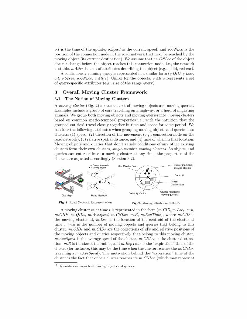
We employ a similar motion model as in [22, 34], where moving objects areassumed to move in a piecewise linear manner in a road network (Fig. 1). Theirmovements are constrained by roads, which are connected by network nodes,also known as connection nodes2.

We assume moving objects’ location updates arrive via data streams andhave the following form (o.OID, o.Loct, o.t, o.Speed, o.CNLoc, o.Attrs), whereo.OID is the id of the moving object, o.Loct is the position of the moving object,

2Our solution relies on the fact that objects have common spatio-temporal properties indepen-dent of whether objects move in the network or not, and is applicable to both constrained andunconstrained moving objects.

o.t is the time of the update, o.Speed is the current speed, and o.CNLoc is theposition of the connection node in the road network that next be reached by themoving object (its current destination). We assume that an CNLoc of the objectdoesn’t change before the object reaches this connection node, i.e., the networkis stable. o.Attrs is a set of attributes describing the object (e.g., child, red car).

A continuously running query is represented in a similar form (q.QID, q.Loct,q.t, q.Speed, q.CNLoc, q.Attrs). Unlike for the objects, q.Attrs represents a setof query-specific attributes (e.g., size of the range query)

3 Overall Moving Cluster Framework

3.1 The Notion of Moving Clusters

A moving cluster (Fig. 2) abstracts a set of moving objects and moving queries.Examples include a group of cars travelling on a highway, or a herd of migratinganimals. We group both moving objects and moving queries into moving clustersbased on common spatio-temporal properties i.e., with the intuition that thegrouped entities3 travel closely together in time and space for some period. Weconsider the following attributes when grouping moving objects and queries intoclusters: (1) speed, (2) direction of the movement (e.g., connection node on theroad network), (3) relative spatial distance, and (4) time of when in that location.Moving objects and queries that don’t satisfy conditions of any other existingclusters form their own clusters, single-member moving clusters. As objects andqueries can enter or leave a moving cluster at any time, the properties of thecluster are adjusted accordingly (Section 3.2).

Road NetworkCity Map

- Connection node- Moving object

Fig. 1. Road Network Representation

Centroid

Actual Cluster SizeD

Max Cluster Size

Velocity Vector

Cluster members:moving objects

Cluster members:moving queries

Fig. 2. Moving Cluster in SCUBA

A moving cluster m at time t is represented in the form (m.CID, m.Loct, m.n,m.OIDs, m.QIDs, m.AveSpeed, m.CNLoc, m.R, m.ExpTime), where m.CID isthe moving cluster id, m.Loct is the location of the centroid of the cluster attime t, m.n is the number of moving objects and queries that belong to thiscluster, m.OIDs and m.QIDs are the collections of id’s and relative positions ofthe moving objects and queries respectively that belong to this moving cluster,m.AveSpeed is the average speed of the cluster, m.CNLoc is the cluster destina-tion, m.R is the size of the radius, and m.ExpTime is the “expiration” time of thecluster (for instance, this may be the time when the cluster reaches the m.CNLoctravelling at m.AveSpeed). The motivation behind the “expiration” time of thecluster is the fact that once a cluster reaches its m.CNLoc (which may represent

3By entities we mean both moving objects and queries.

a major road intersection) its members may change their spatio-temporal prop-erties significantly (e.g., move in different directions) and thus no longer belongto the same cluster. Alternate options are possible here (e.g., splitting a movingcluster). We plan to explore this as a part of our future work.

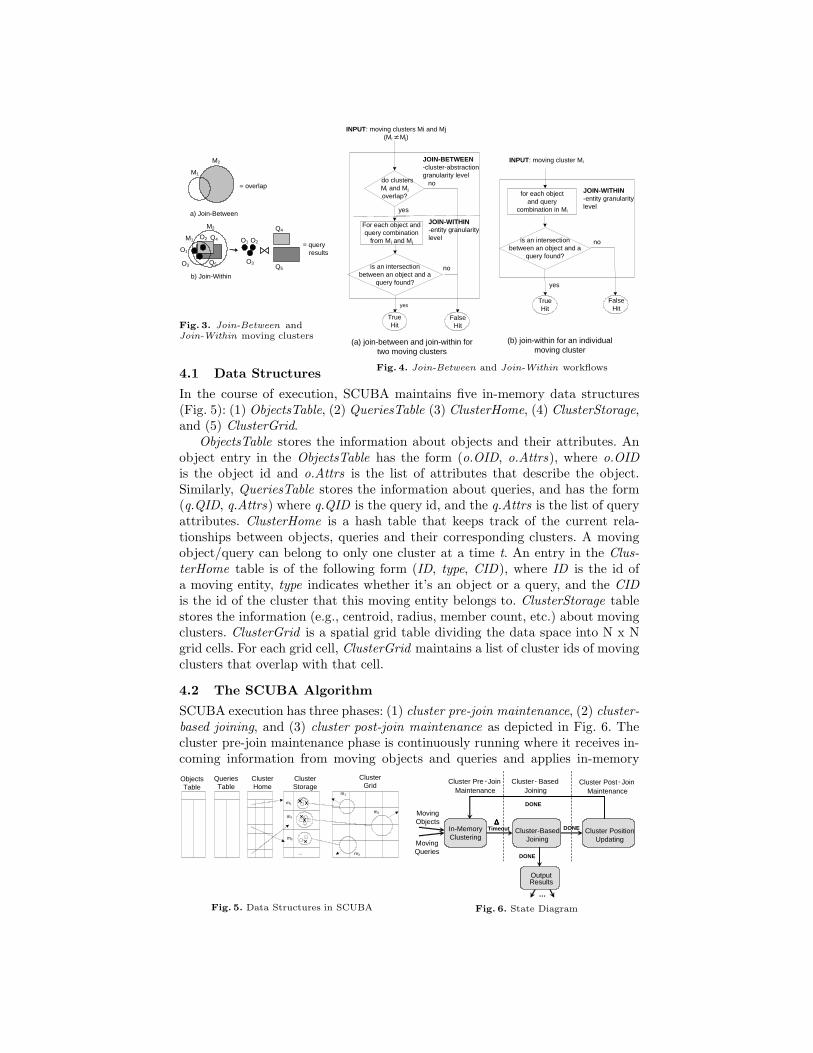
Individual positions of moving objects and queries inside a cluster are repre-sented in a relative form using polar coordinates (with the pole at the centroidof the cluster). For any location update point P its polar coordinates are (r, θ),where r is the radial distance from the centroid, and θ is the the counterclockwiseangle from the x-axis. As time progresses, the center of the cluster might shift,thus making it necessary to transform the relative coordinates of the clustermembers. We maintain a transformation vector for each cluster that records thechanges in position of the centroid between the periodic executions. We refrainfrom constantly updating the relative positions of the cluster members, as thisinfo is not needed, unless a join-within is to be performed (Fig. 3).

We face the challenge that with time clusters may deteriorate [15]. To keepa competitive and high quality clustering (i.e., clusters with compact sizes), weset the following thresholds to limit the sizes and deterioration of the clusters asthe time progresses: (1) distance threshold (ΘD) and (2) speed threshold (ΘS).Distance threshold guarantees that the clustered entities are close to each otherat the time of clustering, while the speed threshold assures that the entitieswill stay close to each other for some time in the future. The thresholds preventdissimilar moving entities from being classified under the same cluster and ensurethat good quality clusters will be formed.

Clusters are dissolved once they reach their destination points. So if thedistance between the location where the cluster has been formed and its des-tination is short, the clustering approach might be quite expensive and not asworthwhile. The same reasoning applies if the average speed of the cluster isvery fast and it thus reaches its destination point very quickly, then forming acluster might not give very little, if any, advantages. In a typical real-life sce-nario though, moving objects can reach relatively high speeds on the larger roads(e.g., highways), where connection nodes would be far apart from each other.On the smaller roads, speed limit, and the proximity of other cars constrains themaximum speed the objects can develop, thus extending the time it takes forthem to reach the connection nodes. These observations support our intuitionthat clustering is applicable to different speed scenarios for moving objects inevery day life.

3.2 Moving Cluster Formation

We adapt an incremental clustering algorithm, similar to the Leader-Followerclustering [8, 16], to create and maintain moving clusters in SCUBA. Incremen-tal clustering allows us not to store all the location updates that are to begrouped into the clusters. So the space requirements are small compared to thenon-incremental algorithms. Also once ∆ expires, SCUBA can immediately pro-ceed with the query execution, without spending any time on re-clustering theentire data set. However, incremental clustering makes local one-at-a time de-cisions and its outcome is in part dependent on the arrival order of updates.

We experimentally evaluate the tradeoff between the execution time and clus-tering quality when clustering location updates incrementally as updates arrivevs. non-incrementally when the entire data set is available (Sec. 6.4).

We now will illustrate using an example of a moving object how movingentities get clustered. A spatial grid index (we will refer to it as ClusterGrid)is used to optimize the process of clustering. When a location update from themoving object o arrives, the following five steps determine the moving cluster itbelongs to:————————————————————————————————————————————Step 1: Use moving object’s position to probe the spatial grid index ClusterGrid to find the movingclusters (Sc) in the proximity of the current location (i.e., clusters that the object can potentiallyjoin).————————————————————————————————————————————Step 2: If there are no clusters in the grid cell (Sc = ∅), then the object forms its own cluster, withthe centroid at the current location of the object, and the radius = 0;————————————————————————————————————————————Step 3: If otherwise, there are clusters that the object can potentially join, we iterate through thelist of the clusters Sc and for each moving cluster mi ∈ Sc check the following properties:

1. Is the moving object moving in the same direction as the cluster mi

(o.CNLoc == mi.CNLoc)?2. Is the distance between the centroid of the cluster and the location update less than the distance

threshold, that is |o.Loct − mi.Loct| ≤ ΘD?3. Is the speed of the moving object less than the speed threshold, that is

|o.Speed − mi.AveSpeed| ≤ ΘS?————————————————————————————————————————————Step 4: If the moving object o satisfies all three conditions in Step 3, then the moving cluster mi

absorbs o, and adjusts its properties based on o’s attributes. The cluster centroid position is ad-justed by considering the new relative position of object o. The average speed gets recomputed. Ifthe distance between the object o and the cluster centroid is greater than the current radius, theradius is increased. Finally, the count of the cluster members is incremented.————————————————————————————————————————————Step 5: If o cannot join any existing cluster (from Step 4), o forms its own moving cluster.————————————————————————————————————————————Critical situations (e.g., each moving cluster contains one object or one big mov-ing cluster contains all moving objects) are rare to happen. If such situation doesin fact occur, then our solution can default to any other state-of-the-art movingobjects processing technique without any savings offered by our solution.

4 Join Algorithm Using Moving Clusters

In this section, we describe the joining methods utilized by SCUBA to minimizethe cost of execution of spatio-temporal queries. The main idea is to groupsimilar objects as well as queries into moving clusters, and then the evaluationof a set of spatio-temporal queries is abstracted as a spatial join, first between themoving clusters (which serves as a filtering step) and then within the movingclusters (Fig. 3). To illustrate the idea, traditionally each individual query isevaluated separately. In the shared execution paradigm the problem of evaluatingnumerous spatio-temporal queries is abstracted as s spatial join between theset of moving objects and queries [39]. While a shared plan allows processingwith only one scan, however objects and queries are still joined individually.With large numbers of objects and queries, this may still create a bottleneckin performance and may cause us to potentially run out of memory. The sharedcluster-based execution groups moving entities into moving clusters and a spatialjoin is performed on all moving clusters. Only if two clusters overlap, we have togo to the individual object/query level of processing, or automatically assumethat objects and queries within those clusters produce join results (Fig. 4).

a) Join-Between

b) Join-Within

= overlap

= query results

M1

M2

M1

M2

O1 O2

O3

Q4

Q5

O1

O2

O3

Q4

Q5

Fig. 3. Join-Between andJoin-Within moving clusters

do clusters Mi and Mj overlap?

INPUT: moving clusters Mi and Mj(Mi Mj)

yes

JOIN-BETWEEN-cluster-abstraction granularity level

JOIN-WITHIN-entity granularity level

is an intersection between an object and a

query found?

For each object and query combination

from Mi and Mj

TrueHit

FalseHit

no

no

yes

INPUT: moving cluster Mi

JOIN-WITHIN-entity granularity level

is an intersection between an object and a

query found?

for each object and query

combination in Mi

TrueHit

no

yes

(a) join-between and join-within for two moving clusters

(b) join-within for an individual moving cluster

FalseHit

Fig. 4. Join-Between and Join-Within workflows4.1 Data Structures

In the course of execution, SCUBA maintains five in-memory data structures(Fig. 5): (1) ObjectsTable, (2) QueriesTable (3) ClusterHome, (4) ClusterStorage,and (5) ClusterGrid.

ObjectsTable stores the information about objects and their attributes. Anobject entry in the ObjectsTable has the form (o.OID, o.Attrs), where o.OIDis the object id and o.Attrs is the list of attributes that describe the object.Similarly, QueriesTable stores the information about queries, and has the form(q.QID, q.Attrs) where q.QID is the query id, and the q.Attrs is the list of queryattributes. ClusterHome is a hash table that keeps track of the current rela-tionships between objects, queries and their corresponding clusters. A movingobject/query can belong to only one cluster at a time t. An entry in the Clus-terHome table is of the following form (ID, type, CID), where ID is the id ofa moving entity, type indicates whether it’s an object or a query, and the CIDis the id of the cluster that this moving entity belongs to. ClusterStorage tablestores the information (e.g., centroid, radius, member count, etc.) about movingclusters. ClusterGrid is a spatial grid table dividing the data space into N x Ngrid cells. For each grid cell, ClusterGrid maintains a list of cluster ids of movingclusters that overlap with that cell.

4.2 The SCUBA Algorithm

SCUBA execution has three phases: (1) cluster pre-join maintenance, (2) cluster-based joining, and (3) cluster post-join maintenance as depicted in Fig. 6. Thecluster pre-join maintenance phase is continuously running where it receives in-coming information from moving objects and queries and applies in-memory

ClusterHome

m1

m2

m3

ClusterGrid

ClusterStorage

m1

m2

m3

...

ObjectsTable

QueriesTable

Fig. 5. Data Structures in SCUBA

…

DONE

DONE

Moving Objects

DONE

Cluster Pre -Join Maintenance

Cluster - Based Joining

Cluster Post Join Maintenance

∆∆∆∆Timeout

Moving Queries

Output Results

-

In-MemoryClustering

Cluster-BasedJoining

Cluster PositionUpdating

Fig. 6. State Diagram

Algorithm 1 SCUBA()

1: loop

2: //*** CLUSTER PRE-JOIN MAINTENANCE PHASE ***3: Tstart = current time //initialize the execution interval start time4: while (current time - Tstart) < ∆ do

5: if new location update arrived then

6: Cluster moving object o/query q //procedure described in Section 3.2// ∆ expires. Begin evaluation of queries

7: //*** CLUSTER-BASED JOINING PHASE ***8: for c = 0 to MAX GRID CELL do

9: for every moving cluster mL ∈ Gc do

10: for every moving cluster mR ∈ Gc do

11: //if the same cluster, do only join-within12: if (mL == mR) then

13: //do within-join only if the cluster contains members of different types14: if ((mL.OIDs > 0) && (mL.QIDs > 0)) then

15: Call DoWithinClusterJoin(mL ,mL)16: else

17: //do between-join only if 2 clusters contain members of different types18: if ((mL.OIDs > 0) && (mR.QIDs > 0)) ||

((mL.QIDs > 0) && (mR.OIDs > 0)) then

19: if DoBetweenClusterJoin(mL,mR) == TRUE then

20: Call DoWithinClusterJoin(mL ,mR)21: Send new query answers to users22: //*** CLUSTER POST-JOIN MAINTENANCE PHASE ***23: Call PostJoinClustersMaintenance() //do some cluster maintenance

Algorithm 2 DoBetweenClusterJoin(Cluster mL, Cluster mR)

1: //Check if two circular clusters mL and mR overlap2: if ((mL.Loct.x - mR.Loct.x)2 + (mL.Loct.y - mR.Loct.y)2) < (mL.R - mR.R)2 then

3: return TRUE; //the clusters overlap4: else

5: return FALSE; //the clusters don’t overlap

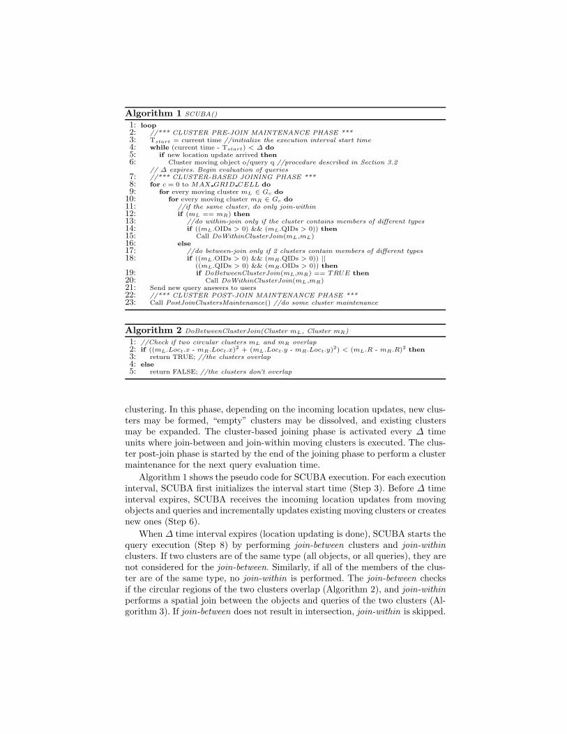
clustering. In this phase, depending on the incoming location updates, new clus-ters may be formed, “empty” clusters may be dissolved, and existing clustersmay be expanded. The cluster-based joining phase is activated every ∆ timeunits where join-between and join-within moving clusters is executed. The clus-ter post-join phase is started by the end of the joining phase to perform a clustermaintenance for the next query evaluation time.

Algorithm 1 shows the pseudo code for SCUBA execution. For each executioninterval, SCUBA first initializes the interval start time (Step 3). Before ∆ timeinterval expires, SCUBA receives the incoming location updates from movingobjects and queries and incrementally updates existing moving clusters or createsnew ones (Step 6).

When ∆ time interval expires (location updating is done), SCUBA starts thequery execution (Step 8) by performing join-between clusters and join-withinclusters. If two clusters are of the same type (all objects, or all queries), they arenot considered for the join-between. Similarly, if all of the members of the clus-ter are of the same type, no join-within is performed. The join-between checksif the circular regions of the two clusters overlap (Algorithm 2), and join-withinperforms a spatial join between the objects and queries of the two clusters (Al-gorithm 3). If join-between does not result in intersection, join-within is skipped.

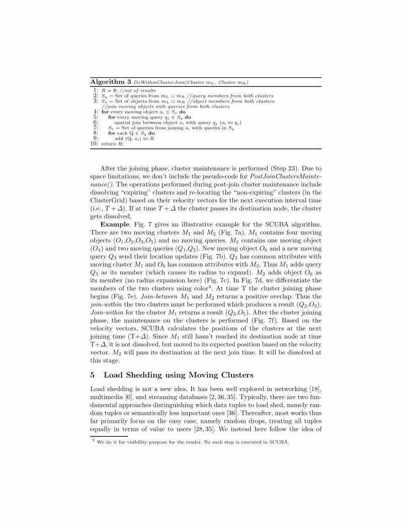
Algorithm 3 DoWithinClusterJoin(Cluster mL, Cluster mR)

1: R = ∅; //set of results2: Sq = Set of queries from mL ∪ mR //query members from both clusters3: So = Set of objects from mL ∪ mR //object members from both clusters

//join moving objects with queries from both clusters4: for every moving object oi ∈ So do

5: for every moving query qj ∈ Sq do

6: spatial join between object oi with query qj (oi ./ qj)7: Sr = Set of queries from joining oi with queries in Sq

8: for each Q ∈ Sq do

9: add (Q, oi) to R10: return R;

After the joining phase, cluster maintenance is performed (Step 23). Due tospace limitations, we don’t include the pseudo-code for PostJoinClustersMainte-nance(). The operations performed during post-join cluster maintenance includedissolving “expiring” clusters and re-locating the “non-expiring” clusters (in theClusterGrid) based on their velocity vectors for the next execution interval time(i.e., T +∆). If at time T +∆ the cluster passes its destination node, the clustergets dissolved.

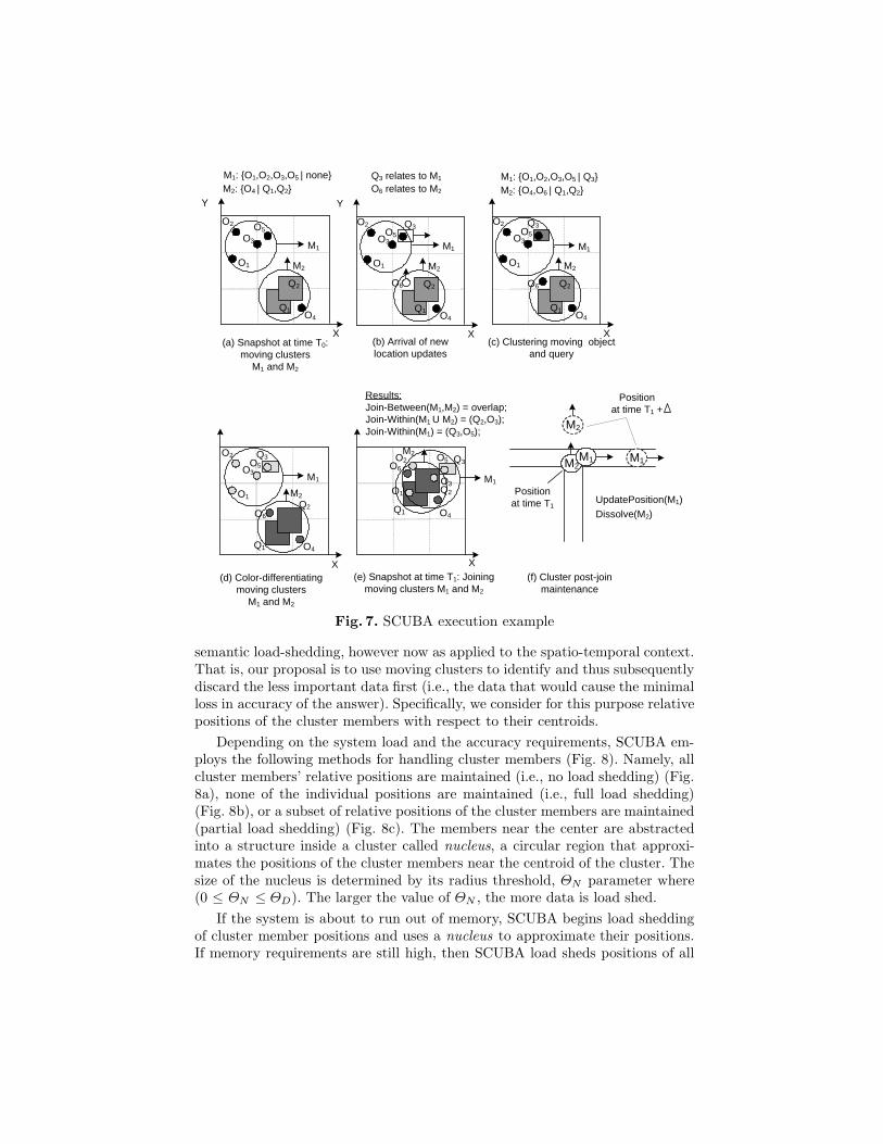
Example. Fig. 7 gives an illustrative example for the SCUBA algorithm.There are two moving clusters M1 and M2 (Fig. 7a). M1 contains four movingobjects (O1,O2,O3,O5) and no moving queries. M2 contains one moving object(O4) and two moving queries (Q1,Q2). New moving object O6 and a new movingquery Q3 send their location updates (Fig. 7b). Q3 has common attributes withmoving cluster M1 and O6 has common attributes with M2. Thus M1 adds queryQ3 as its member (which causes its radius to expand). M2 adds object O6 asits member (no radius expansion here) (Fig. 7c). In Fig. 7d, we differentiate themembers of the two clusters using color4. At time T the cluster joining phasebegins (Fig. 7e). Join-between M1 and M2 returns a positive overlap. Thus thejoin-within the two clusters must be performed which produces a result (Q2,O3).Join-within for the cluster M1 returns a result (Q3,O5). After the cluster joiningphase, the maintenance on the clusters is performed (Fig. 7f). Based on thevelocity vectors, SCUBA calculates the positions of the clusters at the nextjoining time (T+∆). Since M1 still hasn’t reached its destination node at timeT+∆, it is not dissolved, but moved to its expected position based on the velocityvector. M2 will pass its destination at the next join time. It will be dissolved atthis stage.

5 Load Shedding using Moving Clusters

Load shedding is not a new idea. It has been well explored in networking [18],multimedia [6], and streaming databases [2, 36, 35]. Typically, there are two fun-damental approaches distinguishing which data tuples to load shed, namely ran-dom tuples or semantically less important ones [36]. Thereafter, most works thusfar primarily focus on the easy case, namely random drops, treating all tuplesequally in terms of value to users [28, 35]. We instead here follow the idea of

4We do it for visibility purpose for the reader. No such step is executed in SCUBA.

(a) Snapshot at time T0: moving clusters

M1 and M2

X

YM2: {O4 | Q1,Q2}M1: {O1,O2,O3,O5 | none}

M1

O1

O2

O3

O5

M2

O4Q1

Q2

(b) Arrival of new location updates

X

Y

Q3 relates to M1

M1

O1

O2

O3O5

M2

O4Q1

Q2O6

Q3

O6 relates to M2

(c) Clustering moving object and query

X

M2

O4Q1

Q2O6

M2: {O4,O6 | Q1,Q2}M1: {O1,O2,O3,O5 | Q3}

(d) Color-differentiating moving clusters

M1 and M2

X

O6

M2

O4Q1

Q2

Q3

M1

O1

O2

O3O5

(e) Snapshot at time T1: Joining moving clusters M1 and M2

X

O6

M2

O4Q1

Q2

Q3

M1

O1

O2

O3

O5

O1

O2

O3O5

Q3

M1

Results:Join-Between(M1,M2) = overlap;Join-Within(M1 U M2) = (Q2,O3);Join-Within(M1) = (Q3,O5);

M2M1 M1

Position at time T1

Position at time T1 +

M2

(f) Cluster post-join maintenance

Dissolve(M2)

UpdatePosition(M1)

Fig. 7. SCUBA execution example

semantic load-shedding, however now as applied to the spatio-temporal context.That is, our proposal is to use moving clusters to identify and thus subsequentlydiscard the less important data first (i.e., the data that would cause the minimalloss in accuracy of the answer). Specifically, we consider for this purpose relativepositions of the cluster members with respect to their centroids.

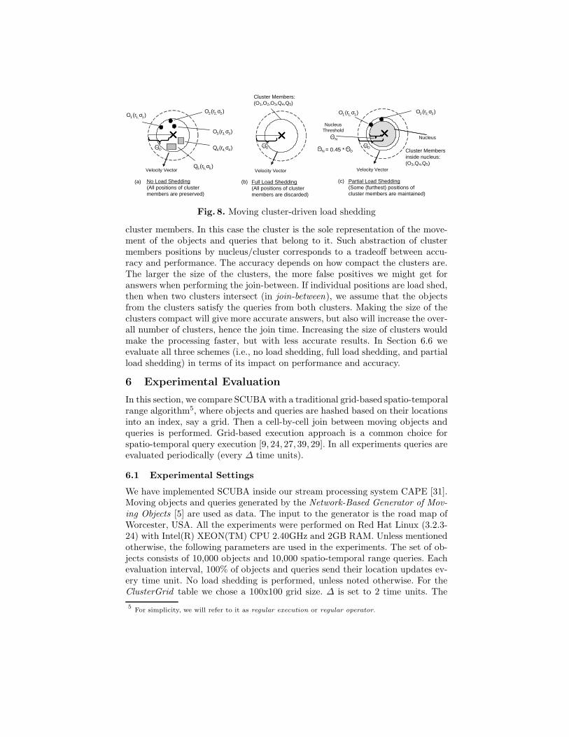
Depending on the system load and the accuracy requirements, SCUBA em-ploys the following methods for handling cluster members (Fig. 8). Namely, allcluster members’ relative positions are maintained (i.e., no load shedding) (Fig.8a), none of the individual positions are maintained (i.e., full load shedding)(Fig. 8b), or a subset of relative positions of the cluster members are maintained(partial load shedding) (Fig. 8c). The members near the center are abstractedinto a structure inside a cluster called nucleus, a circular region that approxi-mates the positions of the cluster members near the centroid of the cluster. Thesize of the nucleus is determined by its radius threshold, ΘN parameter where(0 ≤ ΘN ≤ ΘD). The larger the value of ΘN , the more data is load shed.

If the system is about to run out of memory, SCUBA begins load sheddingof cluster member positions and uses a nucleus to approximate their positions.If memory requirements are still high, then SCUBA load sheds positions of all

O1 (r1,σ1)O2(r2,σ2)

O3(r3,σ3)

Q4(r4,σ4)

Q5 (r5,σ5)

No Load Shedding(All positions of cluster members are preserved)

Velocity Vector

(a)

D

Velocity Vector

Full Load Shedding(All positions of cluster members are discarded)

(b)

Cluster Members:(O1,O2,O3,Q4,Q5)

D

O2(r2,σ2)O1(r1,σ1)

Velocity Vector

Nucleus

Nucleus Threshold

Partial Load Shedding(Some (furthest) positions of cluster members are maintained)

(c)

Cluster Members inside nucleus:(O3,Q4,Q5)

D

N

= 0.45 * DN

Fig. 8. Moving cluster-driven load shedding

cluster members. In this case the cluster is the sole representation of the move-ment of the objects and queries that belong to it. Such abstraction of clustermembers positions by nucleus/cluster corresponds to a tradeoff between accu-racy and performance. The accuracy depends on how compact the clusters are.The larger the size of the clusters, the more false positives we might get foranswers when performing the join-between. If individual positions are load shed,then when two clusters intersect (in join-between), we assume that the objectsfrom the clusters satisfy the queries from both clusters. Making the size of theclusters compact will give more accurate answers, but also will increase the over-all number of clusters, hence the join time. Increasing the size of clusters wouldmake the processing faster, but with less accurate results. In Section 6.6 weevaluate all three schemes (i.e., no load shedding, full load shedding, and partialload shedding) in terms of its impact on performance and accuracy.

6 Experimental Evaluation

In this section, we compare SCUBA with a traditional grid-based spatio-temporalrange algorithm5, where objects and queries are hashed based on their locationsinto an index, say a grid. Then a cell-by-cell join between moving objects andqueries is performed. Grid-based execution approach is a common choice forspatio-temporal query execution [9, 24, 27, 39, 29]. In all experiments queries areevaluated periodically (every ∆ time units).

6.1 Experimental Settings

We have implemented SCUBA inside our stream processing system CAPE [31].Moving objects and queries generated by the Network-Based Generator of Mov-ing Objects [5] are used as data. The input to the generator is the road map ofWorcester, USA. All the experiments were performed on Red Hat Linux (3.2.3-24) with Intel(R) XEON(TM) CPU 2.40GHz and 2GB RAM. Unless mentionedotherwise, the following parameters are used in the experiments. The set of ob-jects consists of 10,000 objects and 10,000 spatio-temporal range queries. Eachevaluation interval, 100% of objects and queries send their location updates ev-ery time unit. No load shedding is performed, unless noted otherwise. For theClusterGrid table we chose a 100x100 grid size. ∆ is set to 2 time units. The

5For simplicity, we will refer to it as regular execution or regular operator.

0

10

20

30

40

50

60

50x50 75x75 100x100 125x125 150x150

REGULAR SCUBA

0

500

1000

1500

2000

50x50 75x75 100x100 125x125 150x150

REGULAR SCUBAT

ime

(in s

ecs)

(a) Join TimeGrid Cell Count Grid Cell Count

Mem

ory

(in M

B)

(b) Memory Consumption

Fig. 9. Varying grid size

distance threshold ΘD equals 100 spatial units, and the speed threshold ΘS isset to 10 (spatial units/time units).

6.2 Varying Grid Cell Size

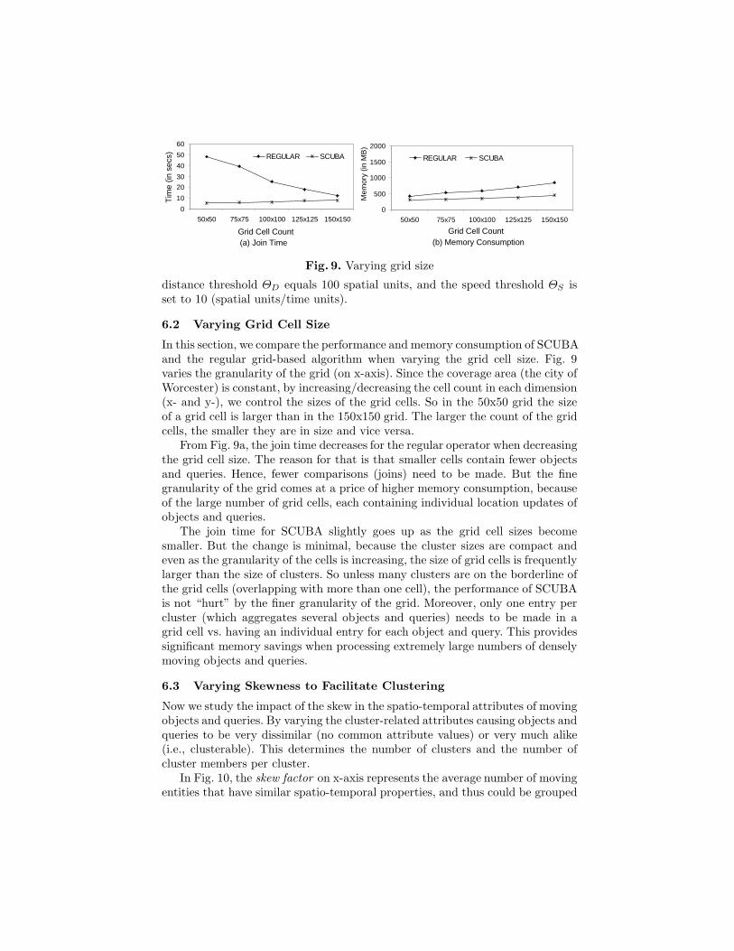
In this section, we compare the performance and memory consumption of SCUBAand the regular grid-based algorithm when varying the grid cell size. Fig. 9varies the granularity of the grid (on x-axis). Since the coverage area (the city ofWorcester) is constant, by increasing/decreasing the cell count in each dimension(x- and y-), we control the sizes of the grid cells. So in the 50x50 grid the sizeof a grid cell is larger than in the 150x150 grid. The larger the count of the gridcells, the smaller they are in size and vice versa.

From Fig. 9a, the join time decreases for the regular operator when decreasingthe grid cell size. The reason for that is that smaller cells contain fewer objectsand queries. Hence, fewer comparisons (joins) need to be made. But the finegranularity of the grid comes at a price of higher memory consumption, becauseof the large number of grid cells, each containing individual location updates ofobjects and queries.

The join time for SCUBA slightly goes up as the grid cell sizes becomesmaller. But the change is minimal, because the cluster sizes are compact andeven as the granularity of the cells is increasing, the size of grid cells is frequentlylarger than the size of clusters. So unless many clusters are on the borderline ofthe grid cells (overlapping with more than one cell), the performance of SCUBAis not “hurt” by the finer granularity of the grid. Moreover, only one entry percluster (which aggregates several objects and queries) needs to be made in agrid cell vs. having an individual entry for each object and query. This providessignificant memory savings when processing extremely large numbers of denselymoving objects and queries.

6.3 Varying Skewness to Facilitate Clustering

Now we study the impact of the skew in the spatio-temporal attributes of movingobjects and queries. By varying the cluster-related attributes causing objects andqueries to be very dissimilar (no common attribute values) or very much alike(i.e., clusterable). This determines the number of clusters and the number ofcluster members per cluster.

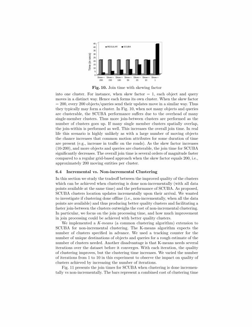
In Fig. 10, the skew factor on x-axis represents the average number of movingentities that have similar spatio-temporal properties, and thus could be grouped

0

5

10

15

20

25

30

35

40

45

Skew =200

Skew =150

Skew =100

Skew =50

Skew =20

Skew =10

Skew =1

REGULAR SCUBA

Tim

e (in

sec

s)Fig. 10. Join time with skewing factor

into one cluster. For instance, when skew factor = 1, each object and querymoves in a distinct way. Hence each forms its own cluster. When the skew factor= 200, every 200 objects/queries send their updates move in a similar way. Thusthey typically may form a cluster. In Fig. 10, when not many objects and queriesare clusterable, the SCUBA performance suffers due to the overhead of manysingle-member clusters. Thus more join-between clusters are performed as thenumber of clusters goes up. If many single member clusters spatially overlap,the join-within is performed as well. This increases the overall join time. In reallife this scenario is highly unlikely as with a large number of moving objectsthe chance increases that common motion attributes for some duration of timeare present (e.g., increase in traffic on the roads). As the skew factor increases(10-200), and more objects and queries are clusterable, the join time for SCUBAsignificantly decreases. The overall join time is several orders of magnitude fastercompared to a regular grid-based approach when the skew factor equals 200, i.e.,approximately 200 moving entities per cluster.

6.4 Incremental vs. Non-incremental Clustering

In this section we study the tradeoff between the improved quality of the clusterswhich can be achieved when clustering is done non-incrementally (with all datapoints available at the same time) and the performance of SCUBA. As proposed,SCUBA clusters location updates incrementally upon their arrival. We wantedto investigate if clustering done offline (i.e., non-incrementally, when all the datapoints are available) and thus producing better quality clusters and facilitating afaster join-between the clusters outweighs the cost of non-incremental clustering.In particular, we focus on the join processing time, and how much improvementin join processing could be achieved with better quality clusters.

We implemented a K-means (a common clustering algorithm) extension toSCUBA for non-incremental clustering. The K-means algorithm expects thenumber of clusters specified in advance. We used a tracking counter for thenumber of unique destinations of objects and queries for a rough estimate of thenumber of clusters needed. Another disadvantage is that K-means needs severaliterations over the dataset before it converges. With each iteration, the qualityof clustering improves, but the clustering time increases. We varied the numberof iterations from 1 to 10 in this experiment to observe the impact on quality ofclusters achieved by increasing the number of iterations.

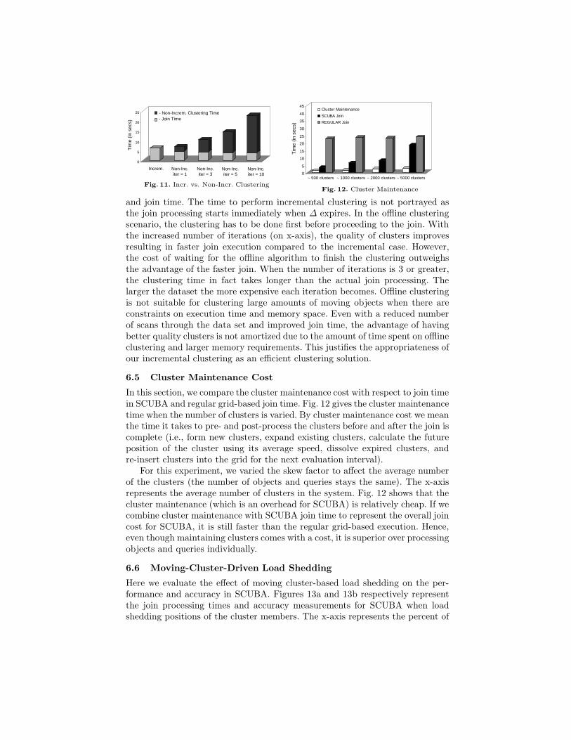
Fig. 11 presents the join times for SCUBA when clustering is done incremen-tally vs non-incrementally. The bars represent a combined cost of clustering time

0

5

10

15

20

25 Offline Clustering Time

Join Time

Tim

e (in

sec

s)

Increm. Non-Inc.iter = 1

Non-Inc.iter = 3

Non-Inc.iter = 5

Non-Inc.iter = 10

- Non-Increm. Clustering Time- Join Time

Fig. 11. Incr. vs. Non-Incr. Clustering

0

5

10

15

20

25

30

35

40

45

~ 500 clusters ~ 1000 clusters ~ 2000 clusters ~ 5000 clusters

Cluster Maintenance

SCUBA Join

REGULAR Join

Tim

e (in

sec

s)

Fig. 12. Cluster Maintenance

and join time. The time to perform incremental clustering is not portrayed asthe join processing starts immediately when ∆ expires. In the offline clusteringscenario, the clustering has to be done first before proceeding to the join. Withthe increased number of iterations (on x-axis), the quality of clusters improvesresulting in faster join execution compared to the incremental case. However,the cost of waiting for the offline algorithm to finish the clustering outweighsthe advantage of the faster join. When the number of iterations is 3 or greater,the clustering time in fact takes longer than the actual join processing. Thelarger the dataset the more expensive each iteration becomes. Offline clusteringis not suitable for clustering large amounts of moving objects when there areconstraints on execution time and memory space. Even with a reduced numberof scans through the data set and improved join time, the advantage of havingbetter quality clusters is not amortized due to the amount of time spent on offlineclustering and larger memory requirements. This justifies the appropriateness ofour incremental clustering as an efficient clustering solution.

6.5 Cluster Maintenance Cost

In this section, we compare the cluster maintenance cost with respect to join timein SCUBA and regular grid-based join time. Fig. 12 gives the cluster maintenancetime when the number of clusters is varied. By cluster maintenance cost we meanthe time it takes to pre- and post-process the clusters before and after the join iscomplete (i.e., form new clusters, expand existing clusters, calculate the futureposition of the cluster using its average speed, dissolve expired clusters, andre-insert clusters into the grid for the next evaluation interval).

For this experiment, we varied the skew factor to affect the average numberof the clusters (the number of objects and queries stays the same). The x-axisrepresents the average number of clusters in the system. Fig. 12 shows that thecluster maintenance (which is an overhead for SCUBA) is relatively cheap. If wecombine cluster maintenance with SCUBA join time to represent the overall joincost for SCUBA, it is still faster than the regular grid-based execution. Hence,even though maintaining clusters comes with a cost, it is superior over processingobjects and queries individually.

6.6 Moving-Cluster-Driven Load Shedding

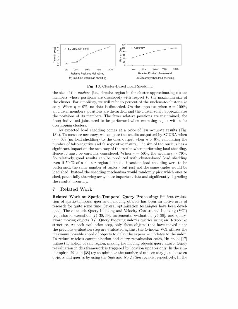
Here we evaluate the effect of moving cluster-based load shedding on the per-formance and accuracy in SCUBA. Figures 13a and 13b respectively representthe join processing times and accuracy measurements for SCUBA when loadshedding positions of the cluster members. The x-axis represents the percent of

01234567

SCUBA Join Time

0

20

40

60

80

100

120

Accuracy

Tim

e (in

sec

s)

Per

cent

(%

)

0% 25% 50% 75% 100%

Relative Positions Maintained

0% 25% 50% 75% 100%

Relative Positions Maintained

(a) Join time when load shedding (b) Accuracy when load shedding

Fig. 13. Cluster-Based Load Shedding

the size of the nucleus (i.e., circular region in the cluster approximating clustermembers whose positions are discarded) with respect to the maximum size ofthe cluster. For simplicity, we will refer to percent of the nucleus-to-cluster sizeas η. When η = 0%, no data is discarded. On the opposite, when η = 100%,all cluster members’ positions are discarded, and the cluster solely approximatesthe positions of its members. The fewer relative positions are maintained, thefewer individual joins need to be performed when executing a join-within foroverlapping clusters.

As expected load shedding comes at a price of less accurate results (Fig.13b). To measure accuracy, we compare the results outputted by SCUBA whenη = 0% (no load shedding) to the ones output when η > 0%, calculating thenumber of false-negative and false-positive results. The size of the nucleus has asignificant impact on the accuracy of the results when performing load shedding.Hence it must be carefully considered. When η = 50%, the accuracy ≈ 79%.So relatively good results can be produced with cluster-based load sheddingeven if 50 % of a cluster region is shed. If random load shedding were to beperformed, the same number of tuples - but just not the same tuples would beload shed. Instead the shedding mechanism would randomly pick which ones toshed, potentially throwing away more important data and significantly degradingthe results’ accuracy.

7 Related Work

Related Work on Spatio-Temporal Query Processing: Efficient evalua-tion of spatio-temporal queries on moving objects has been an active area ofresearch for quite some time. Several optimization techniques have been devel-oped. These include Query Indexing and Velocity Constrained Indexing (VCI)[29], shared execution [24, 38, 39], incremental evaluation [24, 39], and query-aware moving objects [17]. Query Indexing indexes queries using an R-tree-likestructure. At each evaluation step, only those objects that have moved sincethe previous evaluation step are evaluated against the Q-index. VCI utilizes themaximum possible speed of objects to delay the expensive updates to the index.To reduce wireless communication and query reevaluation costs, Hu et. al [17]utilize the notion of safe region, making the moving objects query aware. Queryreevaluation in this framework is triggered by location updates only. In the sim-ilar spirit [29] and [38] try to minimize the number of unnecessary joins betweenobjects and queries by using the Safe and No-Action regions respectively. In the

latter case, the authors combine it with different join policies to filter out theobjects and queries that are guaranteed not to join.

The scalability in spatio-temporal query processing has been addressed in [11,23, 24, 29, 39]. In a distributed environment, such as MobiEyes [11], part of thequery processing is send to the clients. The limitations of this approach is thatthe devices may not have enough battery power and memory capacity to performthe complex computations. The shared execution paradigm as means to achievescalability has been used in SINA [24] for continuous spatio-temporal rangequeries, and in SEA-CNN [39] for continuous spatio-temporal kNN queries. Ourstudy falls into this category and distinguishes itself from these previous worksby focusing on utilizing moving clusters abstracting similar moving entities tooptimize the execution and minimize the individual processing.

Related Work on Clustering: Clustering has been an active field for over 20years [1, 25, 41]. Previous work typically uses clustering to analyze data to findinteresting patterns. We instead apply clustering as means to achieve scalableprocessing of continuous queries on moving objects. To the best of our knowl-edge, this is the first work to use clustering for shared execution optimization ofcontinuous queries on spatio-temporal data streams.

In this work we considered clustering algorithms in which clusters have a dis-tinguished point, a center. The commonly used clustering algorithm for such clus-tering, k-means, is described in [8, 13, 30]. Our concentration was on incrementalclustering algorithms only [4], [7], and [40]. Some of the published clustering algo-rithms for an incremental clustering of data streams include BIRCH[41], COB-WEB [10], STREAM [12, 26], Fractal Clustering [3], and the Leader-Follower(LF) [16]. Clustering analysis is a well researched area, and due to space limita-tions we do not discuss all of the clustering algorithms available. For an elaboratesurvey on clustering, readers are referred to [19]. In our work, we adapt an incre-mental clustering algorithm, similar to the Leader-Follower clustering [16]. Theextensibility, running time and the computational complexity of this algorithmis such that makes it attractive for processing streaming data.

Clustering of spatio-temporal data has been explored to a limited degree in[21]. This work [21] concentrates on discovering moving clusters using historictrajectories of the moving objects. The algorithms proposed assume that alldata is available. Our work instead clusters moving entities at run-time andutilizes moving clusters to solve a completely different problem, namely, efficientprocessing of continuous spatio-temporal queries.

8 Conclusions and Future Work

In this paper, we propose a unique algorithm for efficient processing of largenumbers of spatio-temporal queries on moving objects termed SCUBA. SCUBAcombines motion clustering with shared execution for query execution optimiza-tion. Given a set of moving objects and queries, SCUBA groups them into movingclusters based on common spatio-temporal attributes. To optimize the join exe-cution, SCUBA performs a two-step join execution process by first pre-filteringa set of moving clusters that could produce potential results in the join-between

moving clusters stage and then proceeding with the individual join-within exe-cution on those selected moving clusters. Comprehensive experiments show thatthe performance of SCUBA is better than traditional grid-based approach wheremoving entities are processed individually. In particular the experiments demon-strate that SCUBA: (1) facilitates efficient execution of queries on moving ob-jects that have common spatio-temporal attributes, (2) has low cluster main-tenance/overhead cost, and (3) naturally facilitates load shedding using motionclusters while optimizing the processing time with minimal degradation in resultquality. We believe our work is the first to utilize motion clustering to optimizethe execution of continuous queries on spatio-temporal data streams. As futurework, we plan to further refine and validate moving cluster-driven load shedding,enhance SCUBA to produce results incrementally and explore further throughadditional experimentation.

References

1. R. Agrawal and et. al. Automatic subspace clustering of high dimensional data fordata mining applications. In SIGMOD, pages 94–105, 1998.

2. B. Babcock, M. Datar, and R. Motwani. Load shedding techniques for data streamsystems, 2003.

3. D. Barbara. Chaotic mining: Knowledge discovery using the fractal dimension. InSIGMOD Workshop on Data Mining and Knowl. Discovery, 1999.

4. D. Barbara. Requirements for clustering data streams. SIGKDD Explorations,3(2):23–27, 2002.

5. T. Brinkhoff. A framework for generating network-based moving objects. GeoIn-

formatica, 6(2):153–180, 2002.6. C. L. Compton and D. L. Tennenhouse. Collaborative load shedding for media-

based applications. In Int. Conf. on Multimedia Computing and Systems, 1994.7. P. Domingos and G. Hulten. Catching up with the data: Research issues in mining

data streams. In DMKD, 2001.8. R. O. Duda, P. E. Hart, and D. G. Stork. Pattern Classification. Wiley-Interscience

Publication, 2000.9. H. G. Elmongui, M. F. Mokbel, and W. G. Aref. Spatio-temporal histograms. In

SSTD, 2005.10. D. H. Fisher. Iterative optimization and simplification of hierarchical clusterings.

CoRR, cs.AI/9604103, 1996.11. B. Gedik and L. Liu. Mobieyes: Distributed processing of continuously moving

queries on moving objects in a mobile system. In EDBT, pages 67–87, 2004.12. S. Guha, N. Mishra, R. Motwani, and L. O’Callaghan. Clustering data streams.

In FOCS, pages 359–366, 2000.13. S. K. Gupta, K. S. Rao, and V. Bhatnagar. K-means clustering algorithm for

categorical attributes. In DaWaK, pages 203–208, 1999.14. S. E. Hambrusch, C.-M. Liu, W. G. Aref, and S. Prabhakar. Query processing in

broadcasted spatial index trees. In SSTD, pages 502–521, 2001.15. S. Har-Peled. Clustering motion. In FOCS ’01: Proceedings of the 42nd IEEE

symposium on Foundations of Computer Science, page 84, 2001.16. J. A. Hartigan. Clustering Algorithms. John Wiley and Sons, 1975.17. H. Hu, J. Xu, and D. L. Lee. A generic framework for monitoring continuous

spatial queries over moving objects. In SIGMOD, 2005.

18. V. Jacobson. Congestion avoidance and control. SIGCOMM Comput. Commun.

Rev., 25(1):157–187, 1995.19. A. K. Jain, M. N. Murthy, and P. J. Flynn. Data clustering: A review. Technical

Report MSU-CSE-00-16, Dept. of CS, Michigan State University, 2000.20. D. V. Kalashnikov and et. al. Main memory evaluation of monitoring queries over

moving objects. Distrib. Parallel Databases, 15(2), 2004.21. P. Kalnis, N. Mamoulis, and S. Bakiras. On discovering moving clusters in spatio-

temporal data. In SSTD05, 2005.22. Y. Li, J. Han, and J. Yang. Clustering moving objects. In KDD, pages 617–622,

2004.23. M. F. Mokbel and et. al. Towards scalable location-aware services: requirements

and research issues. In GIS, pages 110–117, 2003.24. M. F. Mokbel, X. Xiong, and W. G. Aref. Sina: Scalable incremental processing

of continuous queries in spatio-temporal databases. In SIGMOD, pages 623–634,2004.

25. R. T. Ng and J. Han. Efficient and effective clustering methods for spatial datamining. In VLDB, pages 144–155, 1994.

26. L. O’Callaghan and et. al. Streaming-data algorithms for high-quality clustering.In ICDE, page 685, 2002.

27. D. Papadias and et. al. Conceptual partitioning: An efficient method for continuousnearest neighbor monitoring. In SIGMOD, 2005.

28. Y. C. Philip. Loadstar: A load shedding scheme for classifying data streams.29. S. Prabhakar and et.al. Query indexing and velocity constrained indexing: Scalable

techniques for continuous queries on moving objects. IEEE Trans. Computers,51(10), 2002.

30. E. M. Rasmussen. Clustering algorithms. In Information Retrieval: Data Structures

& Algorithms, pages 419–442. 1992.31. E. A. Rundensteiner, L. Ding, and et.al. Cape: Continuous query engine with

heterogeneous-grained adaptivity. In VLDB, pages 1353–1356, 2004.32. S. Saltenis, C. S. Jensen, S. T. Leutenegger, and M. A. Lopez. Indexing the

positions of continuously moving objects. In SIGMOD, pages 331–342, 2000.33. A. P. Sistla, O. Wolfson, S. Chamberlain, and S. Dao. Modeling and querying

moving objects. In ICDE, pages 422–432, 1997.34. Y. Tao and D. Papadias. Time-parameterized queries in spatio-temporal databases.

In SIGMOD, pages 334–345, 2002.35. N. Tatbul. Qos-driven load shedding on data streams. In EDBT ’02: Proceedings

of the Worshops XMLDM, MDDE, and YRWS on XML-Based Data Management

and Multimedia Engineering-Revised Papers, London, UK, 2002. Springer-Verlag.36. N. Tatbul, U. Cetintemel, S. B. Zdonik, M. Cherniack, and M. Stonebraker. Load

shedding in a data stream manager. In VLDB, pages 309–320, 2003.37. J. Tayeb, O. Ulusoy, and O. Wolfson. A quadtree-based dynamic attribute indexing

method. Comput. J., 41(3):185–200, 1998.38. X. Xiong and M. F. M. et.al. Scalable spatio-temporal continuous query processing

for location-aware services. In SSDBM, pages 317–, 2004.39. X. Xiong, M. F. Mokbel, and W. G. Aref. Sea-cnn: Scalable processing of con-

tinuous k-nearest neighbor queries in spatio-temporal databases. In ICDE, pages643–654, 2005.

40. N. Ye and X. Li. A scalable, incremental learning algorithm for classificationproblems. Comput. Ind. Eng., 43(4):677–692, 2002.

41. T. Zhang, R. Ramakrishnan, and M. Livny. Birch: An efficient data clusteringmethod for very large databases. In SIGMOD, pages 103–114, 1996.