1 23

Heat and Mass TransferWärme- und Stoffübertragung ISSN 0947-7411Volume 51Number 6 Heat Mass Transfer (2015) 51:875-887DOI 10.1007/s00231-014-1465-3

Second law analysis and optimization ofa parabolic trough receiver tube for directsteam generation

H. C. Nolte, T. Bello-Ochende &J. P. Meyer

1 23

Your article is protected by copyright and

all rights are held exclusively by Springer-

Verlag Berlin Heidelberg. This e-offprint is

for personal use only and shall not be self-

archived in electronic repositories. If you wish

to self-archive your article, please use the

accepted manuscript version for posting on

your own website. You may further deposit

the accepted manuscript version in any

repository, provided it is only made publicly

available 12 months after official publication

or later and provided acknowledgement is

given to the original source of publication

and a link is inserted to the published article

on Springer's website. The link must be

accompanied by the following text: "The final

publication is available at link.springer.com”.

1 3

Heat Mass Transfer (2015) 51:875–887DOI 10.1007/s00231-014-1465-3

ORIGINAL

Second law analysis and optimization of a parabolic trough receiver tube for direct steam generation

H. C. Nolte · T. Bello‑Ochende · J. P. Meyer

Received: 4 January 2014 / Accepted: 22 November 2014 / Published online: 11 December 2014 © Springer-Verlag Berlin Heidelberg 2014

seen that higher operating pressures are more advantageous when the entropy generation minimization is considered in conjunction with the work output.

List of symbolsA Area (m2)As Tube exposed heat transfer area (m2)CR Concentration ratioD Diameter (m)E Exergy (W)f Friction factorG Mass velocity (kg/m2 s)h Heat transfer coefficient [W/(m2 K)]Ib Solar beam radiation (W/m2)k Thermal conductivity [W/(m K)]L Length (m)m Mass flow rate (kg/s)Nu Nusselt numberP Pressure (Pa)Pr Prandtl numberQ Heat (W)Re Reynolds numberSgen Total entropy generation (W/K)Sgen,dT Entropy generation due to finite temperature dif-

ferences (W/K)Sgen,dP Entropy generation due to fluid friction (W/K)Sr Reflected solar energy (W/m2)T Temperature (°C or K)V Velocity (m/s)Wa Aperture area (m)x Quality (% or fraction)

Greek symbolsε Emissivityεvoid Void fraction

Abstract Entropy generation in the receiver tube of a parabolic trough solar collector can mainly be attributed to the fluid friction and finite temperature differences. The contribution of each of these components is investigated under different circumstances. Mass flow rates, tube diam-eters and operating pressures are investigated to obtain good guidelines for receiver tube and plant design. Oper-ating pressures between 3 MPa (saturation temperature of 233.9 °C) and 9 MPa (saturation temperature of 303.3 °C) were investigated. Results show that small diameters can result in excessive fluid friction, especially when the mass flow rates are high. For most cases, tube diameters beyond 20 mm will exclusively be subject to entropy generation due to finite temperature differences, and entropy generation due to fluid friction will be small to negligible. Increasing the concentration ratio will decrease entropy generation, due to a higher heat flux per unit meter. This will ultimately result in shorter receiver tube lengths. From a simulated annealing optimization it was seen that if the diameter is increased, the entropy generation can be lowered, provided that the con-centration ratio is kept constant. However, beyond a certain point gains in minimizing the entropy generation become negligible. The optimal operating pressure will generally increase if the mass flow rate is increased. Finally it was

H. C. Nolte · J. P. Meyer Department of Mechanical and Aeronautical Engineering, University of Pretoria, Private Bag X20, Hatfield 0028, South Africae-mail: henriettenolte@yahoo.com

J. P. Meyer e-mail: joshua.meyer@up.ac.za

T. Bello-Ochende (*) Department of Mechanical Engineering, University of Cape Town, Private Bag X3, Rondebosch 7701, South Africae-mail: tunde.bello-ochende@uct.ac.za

Author's personal copy

876 Heat Mass Transfer (2015) 51:875–887

1 3

ηopt Optical efficiency (%)μ Dynamic viscosity (kg/m s)v Local specific volume (m3/kg)ρ Density (kg/m3)σ Stefan–Boltzmann constant [W/(m2 K4)]Φ2 Two-phase flow multiplier

Subscriptsamb Ambientcb Convective boilingcond Conductionconv Convectiondes Destroyedfluid Working fluidG Vapourg Glassgi Glass innergo Glass outerin InletL Liquidnb Nucleate boilingout Outletr Receiverrad Radiationri Receiver innerro Receiver outersky Effective skysun Apparent suntp Two-phasewind Wind

1 Introduction

Numerous experimental and comparative investigations have been made concerning parabolic trough technol-ogy [1–3]. Parabolic trough technology can use water as a working fluid. If water is used, only one cycle is incor-porated and the superheated steam is eventually passed through a turbine to produce work. The process of heating liquid water to superheated steam in the receiver is also known as direct steam generation or DSG [1]. Odeh et al. [4] investigated the thermal performance of a parabolic trough collector by developing an efficiency equation in terms of the receiver wall temperature rather than the fluid bulk mean temperature. This was done so that the model could be used for different working fluids. Forristall [5] implemented a heat transfer model into Engineering Equa-tion Solver (EES) to investigate the performance of a para-bolic trough receiver. Roesle et al. [6] numerically inves-tigated the heat loss from a parabolic trough receiver tube with an active vacuum system by using computational fluid

dynamics (CFD) and Monte Carlo ray tracing software. However, a second law analysis was not conducted in these models.

Koroneos et al. [7] conducted an exergy analysis of solar, wind as well as geothermal energy. Their research showed that the exergy lost in the receiver–collector sub-system is highest due to greater quality losses compared with the heat engine subsystem. The same conclusions were drawn by Singh et al. [8]. They concluded that the condenser component as well as the receiver component is responsible for the major exergy destruction where the receiver losses are of high quality. Since the exergy losses in the receiver component is of high quality the process of DSG in the receiver is the focus of this work. Entropy gen-eration in the receiver tube can be attributed to fluid friction (Sgen,dp) as well as finite temperature differences (Sgen,dt) [9]. Ratts et al. [10] used entropy generation minimisation to obtain an optimal Reynolds number for turbulent flow, as well as laminar flow. The investigation was extended for non-circular ducts. Sahin [11] explored entropy generation in a smooth duct subject to a constant wall temperature in the turbulent regime. Furthermore, the validity of a constant viscosity assumption was investigated and it was found to be valid for water when the viscosity variations are small. Revellin et al. [12] investigated the local entropy genera-tion for two-phase flow by considering a separated flow model as well as a mixture model. The study also investi-gates the effect of heat transfer enhancement and found that heat transfer enhancement can be beneficial at low mass velocities but not necessarily at high mass velocities. Often when attempting to minimize the entropy generation in a tube, conditions that would minimise the fluid friction com-ponent will increase the temperature difference (heat loss) component, therefore it is of importance to identify design guidelines that will result in optimality.

Parabolic trough technology incorporating DSG can reach temperatures up to 400 °C and pressures up to10 MPa [1, 13]. Operating temperatures are not as high as for 3D focussing collectors, but can be well above ambi-ent. At temperatures significantly higher than ambient, the receiver will be subject to large heat losses. Uneven heat-ing or stratified flow can cause bending of the receiver tube. This can be detrimental, since bending can lead to breakage of the glass cover. The vacuum covering is very effective in retaining the heat, provided that it is maintained correctly.

In this research a second law analysis is used to optimise the receiver tube. To conduct the second law analysis a first law analysis is performed to solve the fluid temperature, receiver temperature and glass cover temperature. An initial sensitivity analysis showed that the main variables of con-cern, that influences the optimality, are the concentration ratio, mass flow, tube diameter and saturation temperature (or operating pressure). Variables such as wind velocity and

Author's personal copy

877Heat Mass Transfer (2015) 51:875–887

1 3

glass cover clearance will affect the entropy generation, but will have low to minimal effect on the minima. The convec-tion on the outer tube is primarily assumed to be forced, in the form of wind. The effects of natural convection on the losses and optimization were not investigated. The model is analytical and attempts to investigate the influence of entropy generation by fluid friction compared to entropy generation due to finite temperature differences. Generally a small scale scenario was investigated. Therefore, for the cases investigated, the turbine work output will be in the range of 50–350 kW.

2 Model and mathematical formulation

2.1 Model

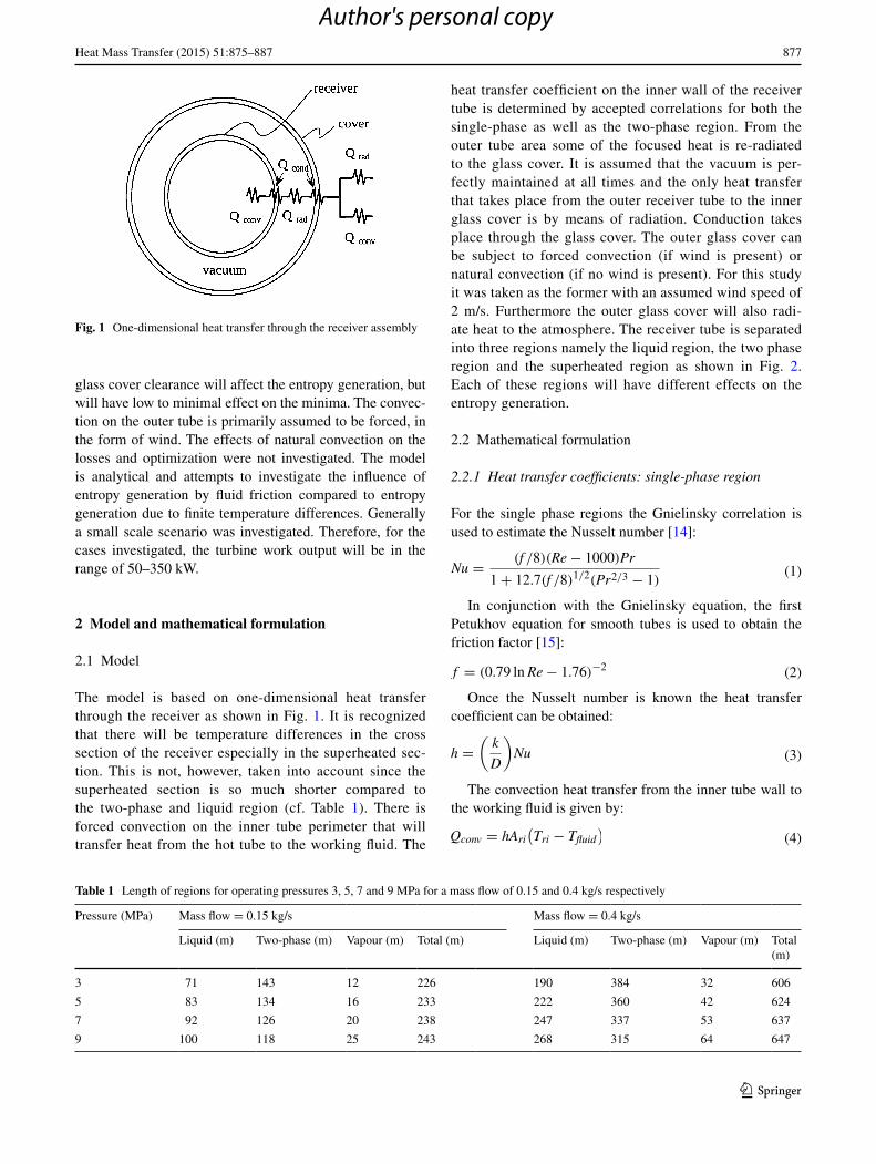
The model is based on one-dimensional heat transfer through the receiver as shown in Fig. 1. It is recognized that there will be temperature differences in the cross section of the receiver especially in the superheated sec-tion. This is not, however, taken into account since the superheated section is so much shorter compared to the two-phase and liquid region (cf. Table 1). There is forced convection on the inner tube perimeter that will transfer heat from the hot tube to the working fluid. The

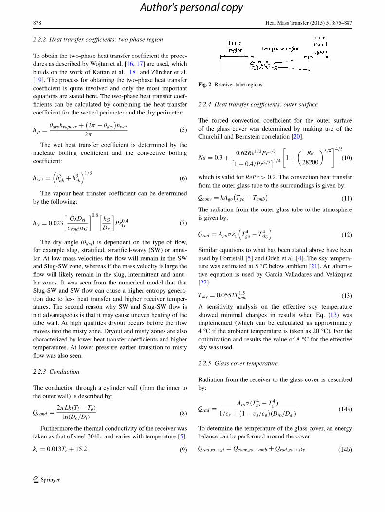
heat transfer coefficient on the inner wall of the receiver tube is determined by accepted correlations for both the single-phase as well as the two-phase region. From the outer tube area some of the focused heat is re-radiated to the glass cover. It is assumed that the vacuum is per-fectly maintained at all times and the only heat transfer that takes place from the outer receiver tube to the inner glass cover is by means of radiation. Conduction takes place through the glass cover. The outer glass cover can be subject to forced convection (if wind is present) or natural convection (if no wind is present). For this study it was taken as the former with an assumed wind speed of 2 m/s. Furthermore the outer glass cover will also radi-ate heat to the atmosphere. The receiver tube is separated into three regions namely the liquid region, the two phase region and the superheated region as shown in Fig. 2. Each of these regions will have different effects on the entropy generation.

2.2 Mathematical formulation

2.2.1 Heat transfer coefficients: single‑phase region

For the single phase regions the Gnielinsky correlation is used to estimate the Nusselt number [14]:

In conjunction with the Gnielinsky equation, the first Petukhov equation for smooth tubes is used to obtain the friction factor [15]:

Once the Nusselt number is known the heat transfer coefficient can be obtained:

The convection heat transfer from the inner tube wall to the working fluid is given by:

(1)Nu =(f /8)(Re− 1000)Pr

1+ 12.7(f /8)1/2(Pr2/3 − 1)

(2)f = (0.79 lnRe− 1.76)−2

(3)h =

(

k

D

)

Nu

(4)Qconv = hAri

(

Tri − Tfluid)

Fig. 1 One-dimensional heat transfer through the receiver assembly

Table 1 Length of regions for operating pressures 3, 5, 7 and 9 MPa for a mass flow of 0.15 and 0.4 kg/s respectively

Pressure (MPa) Mass flow = 0.15 kg/s Mass flow = 0.4 kg/s

Liquid (m) Two-phase (m) Vapour (m) Total (m) Liquid (m) Two-phase (m) Vapour (m) Total (m)

3 71 143 12 226 190 384 32 606

5 83 134 16 233 222 360 42 624

7 92 126 20 238 247 337 53 637

9 100 118 25 243 268 315 64 647

Author's personal copy

878 Heat Mass Transfer (2015) 51:875–887

1 3

2.2.2 Heat transfer coefficients: two‑phase region

To obtain the two-phase heat transfer coefficient the proce-dures as described by Wojtan et al. [16, 17] are used, which builds on the work of Kattan et al. [18] and Zürcher et al. [19]. The process for obtaining the two-phase heat transfer coefficient is quite involved and only the most important equations are stated here. The two-phase heat transfer coef-ficients can be calculated by combining the heat transfer coefficient for the wetted perimeter and the dry perimeter:

The wet heat transfer coefficient is determined by the nucleate boiling coefficient and the convective boiling coefficient:

The vapour heat transfer coefficient can be determined by the following:

The dry angle (θdry) is dependent on the type of flow, for example slug, stratified, stratified-wavy (SW) or annu-lar. At low mass velocities the flow will remain in the SW and Slug-SW zone, whereas if the mass velocity is large the flow will likely remain in the slug, intermittent and annu-lar zones. It was seen from the numerical model that that Slug-SW and SW flow can cause a higher entropy genera-tion due to less heat transfer and higher receiver temper-atures. The second reason why SW and Slug-SW flow is not advantageous is that it may cause uneven heating of the tube wall. At high qualities dryout occurs before the flow moves into the misty zone. Dryout and misty zones are also characterized by lower heat transfer coefficients and higher temperatures. At lower pressure earlier transition to misty flow was also seen.

2.2.3 Conduction

The conduction through a cylinder wall (from the inner to the outer wall) is described by:

Furthermore the thermal conductivity of the receiver was taken as that of steel 304L, and varies with temperature [5]:

(5)htp =θdryhvapour +

(

2π − θdry)

hwet

2π

(6)hwet =(

h3nb + h3cb

)1/3

(7)hG = 0.023

[

GxDri

εvoidµG

]0.8[kG

Dri

]

Pr0.4G

(8)Qcond =2πLk(Ti − To)

ln(Do/Di)

(9)kr = 0.013Tr + 15.2

2.2.4 Heat transfer coefficients: outer surface

The forced convection coefficient for the outer surface of the glass cover was determined by making use of the Churchill and Bernstein correlation [20]:

which is valid for RePr > 0.2. The convection heat transfer from the outer glass tube to the surroundings is given by:

The radiation from the outer glass tube to the atmosphere is given by:

Similar equations to what has been stated above have been used by Forristall [5] and Odeh et al. [4]. The sky tempera-ture was estimated at 8 °C below ambient [21]. An alterna-tive equation is used by Garcia-Valladares and Velázquez [22]:

A sensitivity analysis on the effective sky temperature showed minimal changes in results when Eq. (13) was implemented (which can be calculated as approximately 4 °C if the ambient temperature is taken as 20 °C). For the optimization and results the value of 8 °C for the effective sky was used.

2.2.5 Glass cover temperature

Radiation from the receiver to the glass cover is described by:

To determine the temperature of the glass cover, an energy balance can be performed around the cover:

(10)Nu = 0.3+0.62Re1/2Pr1/3

[

1+ 0.4/Pr2/3]1/4

[

1+

(

Re

28200

)5/8]4/5

(11)Qconv = hAgo

(

Tgo − Tamb)

(12)Qrad = Agoσεg

(

T4go − T4

sky

)

(13)Tsky = 0.0552T1.5amb

(14a)Qrad =Aroσ(T

4ro − T4

gi)

1/εr +(

1− εg/εg)

(Dro/Dgi)

(14b)Qrad,ro→gi = Qconv,go→amb + Qrad,go→sky

Fig. 2 Receiver tube regions

Author's personal copy

879Heat Mass Transfer (2015) 51:875–887

1 3

The radiation through the vacuum, from the receiver to the glass must equal the radiation to the atmosphere from the outer surface as well as the convection losses from the outer surface due to the wind. Such an energy balance usu-ally involves implicitly solving the glass temperatures.

2.2.6 Concentration ratio

The optical efficiency is defined as the reflected solar energy (Sr) over the total solar irradiance (Ib), taken as 1,000 W/m2:

The optical efficiency accounts for inefficiencies due to cover transmittance, absorptance, surface reflectivity and geometry. The optical efficiency was taken as 72 %. The solar radiation falling on the receiver can be obtained by making use of the concentration ration (CR):

The concentration ratio can also be determined from the trough width (Wa) and outer tube diameter (Do):

For a unit length the heat transfer area (As) is given by:

2.2.7 Pressure losses

The single-phase pressure drop was obtained by:

The pressure drop in the two-phase region was deter-mined by making use of the Friedel correlation which uses a two-phase flow multiplier in conjunction with a liquid pressure drop calculation [23, 24]:

where the liquid pressure drop is given by:

2.2.8 Second law analysis

The entropy generated by the finite temperature differences are determined by obtaining the destroyed exergy [21]. The exergy into the receiver is given as:

(15a)ηopt =Sr

Ib

(15b)qsun = CRSr

Qsun = qsunAs

(15c)CR =Wa − Dro

πDro

(15d)As = Droπ

(16)�P = f

(

L

Dri

)

ρV2

2

(17)�Ptp = �PLφ2

(18)�PL = 4fLG2

(

L

Dri

)

1

2ρL

where Tsun in Eq. (19) is the apparent sun temperature with a value of 4,330 K [21]. The exergy into the working fluid is given by:

The destroyed exergy and entropy generation (due to finite temperature differences) is respectively given by:

The entropy generation due to fluid friction can be obtained from [9]:

A similar equation can be used for the two-phase region provided that the local specific volume is used [12]:

3 Numerical model and optimisation

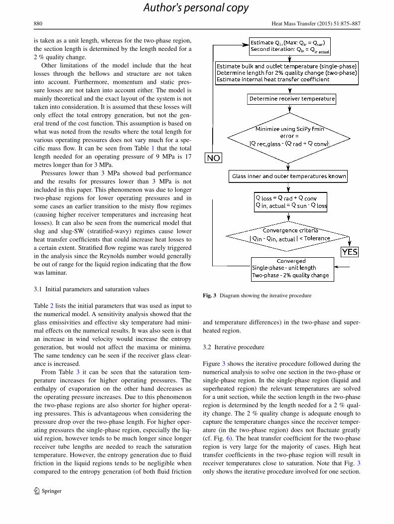
Water is heated from ambient conditions to a superheated state. This means the receiver is subject to both single phase-, as well as two-phase flow. Three regions must be solved: the liquid region, the two-phase region and the superheated region. As the receiver tube gets hotter length-wise, more heat will be lost to the surroundings and changes in fluid properties will be perceived. Coolprop is used to estimate the fluid properties of air and water accurately [25]. A first law analysis is conducted on each unit sec-tion in the single-phase region. The fluid inlet temperature is known from a previous iterative step (cf. Fig. 3). Sub-sequently, the fluid outlet, receiver and cover temperatures are then solved to ultimately estimate the heat losses and exergy destruction for that unit section (single-phase). For the two-phase region the length needed for a 2 % quality change is iteratively calculated. As before (with the single phase region), the quantity of importance is the heat loss. The heat losses are estimated by obtaining the receiver and cover temperature. This process is explained in more detail in the following section. All entropy generation is solved by implementation of Eqs. 1–24 (as stated in Sect. 2) in Python [26]. SciPy [27] packages are used in conjunction with Python for optimisation purposes. Note that the sin-gle-phase regions are handled slightly differently than the two-phase region. For the single phase regions each section

(19)Ein = Qsun

(

1−Tamb

Tsun

)

(20)Eout = Qfluid

(

1−Tamb

Tr

)

(21)Edes = Ein − Eout

(22)Sgen,dT =Edes

Tamb

(23)Sgen,dP =

(

m

ρTin

)

�P

(24)Sgen,dP =

(

mν

Tin

)

�P

Author's personal copy

880 Heat Mass Transfer (2015) 51:875–887

1 3

is taken as a unit length, whereas for the two-phase region, the section length is determined by the length needed for a 2 % quality change.

Other limitations of the model include that the heat losses through the bellows and structure are not taken into account. Furthermore, momentum and static pres-sure losses are not taken into account either. The model is mainly theoretical and the exact layout of the system is not taken into consideration. It is assumed that these losses will only effect the total entropy generation, but not the gen-eral trend of the cost function. This assumption is based on what was noted from the results where the total length for various operating pressures does not vary much for a spe-cific mass flow. It can be seen from Table 1 that the total length needed for an operating pressure of 9 MPa is 17 metres longer than for 3 MPa.

Pressures lower than 3 MPa showed bad performance and the results for pressures lower than 3 MPa is not included in this paper. This phenomenon was due to longer two-phase regions for lower operating pressures and in some cases an earlier transition to the misty flow regimes (causing higher receiver temperatures and increasing heat losses). It can also be seen from the numerical model that slug and slug-SW (stratified-wavy) regimes cause lower heat transfer coefficients that could increase heat losses to a certain extent. Stratified flow regime was rarely triggered in the analysis since the Reynolds number would generally be out of range for the liquid region indicating that the flow was laminar.

3.1 Initial parameters and saturation values

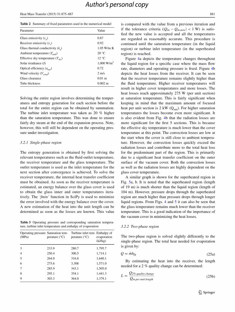
Table 2 lists the initial parameters that was used as input to the numerical model. A sensitivity analysis showed that the glass emissivities and effective sky temperature had mini-mal effects on the numerical results. It was also seen is that an increase in wind velocity would increase the entropy generation, but would not affect the maxima or minima. The same tendency can be seen if the receiver glass clear-ance is increased.

From Table 3 it can be seen that the saturation tem-perature increases for higher operating pressures. The enthalpy of evaporation on the other hand decreases as the operating pressure increases. Due to this phenomenon the two-phase regions are also shorter for higher operat-ing pressures. This is advantageous when considering the pressure drop over the two-phase length. For higher oper-ating pressures the single-phase region, especially the liq-uid region, however tends to be much longer since longer receiver tube lengths are needed to reach the saturation temperature. However, the entropy generation due to fluid friction in the liquid regions tends to be negligible when compared to the entropy generation (of both fluid friction

and temperature differences) in the two-phase and super-heated region.

3.2 Iterative procedure

Figure 3 shows the iterative procedure followed during the numerical analysis to solve one section in the two-phase or single-phase region. In the single-phase region (liquid and superheated region) the relevant temperatures are solved for a unit section, while the section length in the two-phase region is determined by the length needed for a 2 % qual-ity change. The 2 % quality change is adequate enough to capture the temperature changes since the receiver temper-ature (in the two-phase region) does not fluctuate greatly (cf. Fig. 6). The heat transfer coefficient for the two-phase region is very large for the majority of cases. High heat transfer coefficients in the two-phase region will result in receiver temperatures close to saturation. Note that Fig. 3 only shows the iterative procedure involved for one section.

Fig. 3 Diagram showing the iterative procedure

Author's personal copy

881Heat Mass Transfer (2015) 51:875–887

1 3

Solving the entire region involves determining the temper-atures and entropy generation for each section before the total for the entire region can be obtained by summation. The turbine inlet temperature was taken as 20 % higher than the saturation temperature. This was done to ensure fairly dry steam at the end of the expansion process. Note, however, this will still be dependent on the operating pres-sure under investigation.

3.2.1 Single‑phase region

The entropy generation is obtained by first solving the relevant temperatures such as the fluid outlet temperature, the receiver temperature and the glass temperature. The outlet temperature is used as the inlet temperature for the next section after convergence is achieved. To solve the receiver temperature, the internal heat transfer coefficient must be obtained. As soon as the receiver temperature is estimated, an energy balance over the glass cover is used to obtain the glass inner and outer temperatures itera-tively. The ‘fmin’ function in SciPy is used to minimize the error involved with the energy balance over the cover. A new estimation of the heat into the unit length can be determined as soon as the losses are known. This value

is compared with the value from a previous iteration and if the tolerance criteria (|Qin − Qin,new| < 1 W) is satis-fied the new value is accepted and all the temperatures are regarded as reasonably accurate. This procedure is continued until the saturation temperature (in the liquid region) or turbine inlet temperature (in the superheated region) is reached.

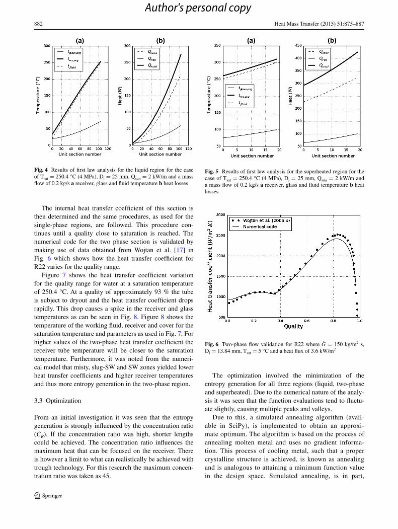
Figure 4a depicts the temperature changes throughout the liquid region for a specific case where the mass flow rate, diameters and operating pressure is fixed. Figure 4b depicts the heat losses from the receiver. It can be seen that the receiver temperature remains slightly higher than the fluid temperature. Higher receiver temperatures will result in higher cover temperatures and more losses. The heat losses reach approximately 275 W (per unit section) at saturation temperature. This is fairly significant when keeping in mind that the maximum amount of focused heat per unit section is 2 kW (Qsun). For higher saturation temperatures the losses become even more significant. It is also evident from Fig. 4b that the radiation losses are more significant for the first 5 sections. This is because the effective sky temperature is much lower than the cover temperature at this point. The convection losses are low at the start when the cover is still close to ambient tempera-ture. However, the convection losses quickly exceed the radiation losses and contribute more to the total heat loss for the predominant part of the region. This is primarily due to a significant heat transfer coefficient on the outer surface of the vacuum cover. Both the convection losses as well as the radiation losses are highly dependent on the glass cover temperature.

A similar graph is shown for the superheated region in Fig. 5a, b. It is noted that the superheated region (length of 19 m) is much shorter than the liquid region (length of 104 m). However, pressure drops through the superheated region are much higher than pressure drops through longer liquid regions. From Figs. 4 and 5 it can also be seen that the glass temperature remains much lower than the receiver temperature. This is a good indication of the importance of the vacuum cover in minimizing the heat losses.

3.2.2 Two‑phase region

The two-phase region is solved slightly differently to the single-phase region. The total heat needed for evaporation is given by:

By estimating the heat into the receiver, the length needed for a 2 % quality change can be determined:

(25a)Q = mhfg

(25b)L =Q2% quality change

Qin per unit length

Table 2 Summary of fixed parameters used in the numerical model

Parameter Value

Glass emissivity (εg) 0.87

Receiver emissivity (εr) 0.92

Glass thermal conductivity (kg) 1.05 W/m K

Ambient temperature (Tamb) 20 °C

Effective sky temperature (Tsky) 12 °C

Solar irradiance (I) 1,000 W/m2

Optical efficiency (ηopt) 0.72

Wind velocity (Vwind) 2 m/s

Glass clearance 0.01 m

Tube thickness 0.002 m

Table 3 Operating pressure and corresponding saturation tempera-ture, turbine inlet temperature and enthalpy of evaporation

Operating pressure (MPa)

Saturation tem-perature (°C)

Turbine inlet tem-perature (°C)

Enthalpy of evaporation (kJ/kg)

3 233.9 280.7 1,795.7

4 250.4 300.5 1,714.1

5 264.0 316.8 1,640.1

6 275.6 3,308 1,571.0

7 285.9 343.1 1,505.0

8 295.1 354.1 1,441.3

9 303.3 364.0 1,379.1

Author's personal copy

882 Heat Mass Transfer (2015) 51:875–887

1 3

The internal heat transfer coefficient of this section is then determined and the same procedures, as used for the single-phase regions, are followed. This procedure con-tinues until a quality close to saturation is reached. The numerical code for the two phase section is validated by making use of data obtained from Wojtan et al. [17] in Fig. 6 which shows how the heat transfer coefficient for R22 varies for the quality range.

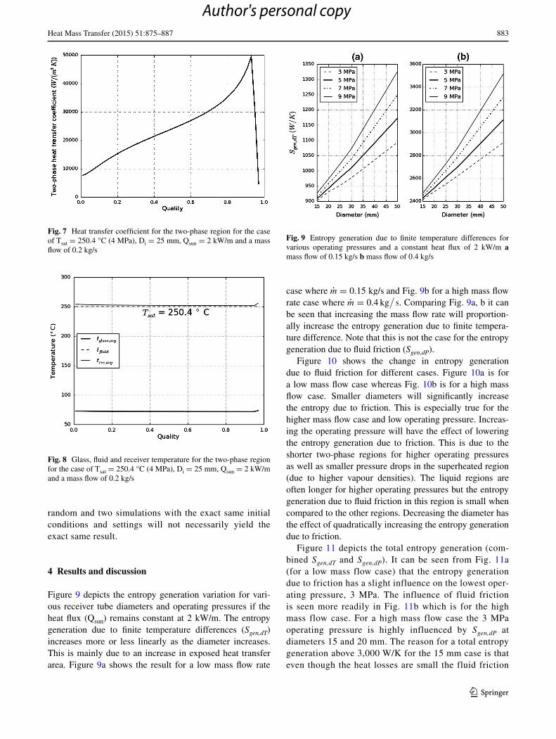
Figure 7 shows the heat transfer coefficient variation for the quality range for water at a saturation temperature of 250.4 °C. At a quality of approximately 93 % the tube is subject to dryout and the heat transfer coefficient drops rapidly. This drop causes a spike in the receiver and glass temperatures as can be seen in Fig. 8. Figure 8 shows the temperature of the working fluid, receiver and cover for the saturation temperature and parameters as used in Fig. 7. For higher values of the two-phase heat transfer coefficient the receiver tube temperature will be closer to the saturation temperature. Furthermore, it was noted from the numeri-cal model that misty, slug-SW and SW zones yielded lower heat transfer coefficients and higher receiver temperatures and thus more entropy generation in the two-phase region.

3.3 Optimization

From an initial investigation it was seen that the entropy generation is strongly influenced by the concentration ratio (CR). If the concentration ratio was high, shorter lengths could be achieved. The concentration ratio influences the maximum heat that can be focused on the receiver. There is however a limit to what can realistically be achieved with trough technology. For this research the maximum concen-tration ratio was taken as 45.

The optimization involved the minimization of the entropy generation for all three regions (liquid, two-phase and superheated). Due to the numerical nature of the analy-sis it was seen that the function evaluations tend to fluctu-ate slightly, causing multiple peaks and valleys.

Due to this, a simulated annealing algorithm (avail-able in SciPy), is implemented to obtain an approxi-mate optimum. The algorithm is based on the process of annealing molten metal and uses no gradient informa-tion. This process of cooling metal, such that a proper crystalline structure is achieved, is known as annealing and is analogous to attaining a minimum function value in the design space. Simulated annealing, is in part,

Fig. 4 Results of first law analysis for the liquid region for the case of Tsat = 250.4 °C (4 MPa), Di = 25 mm, Qsun = 2 kW/m and a mass flow of 0.2 kg/s a receiver, glass and fluid temperature b heat losses

Fig. 5 Results of first law analysis for the superheated region for the case of Tsat = 250.4 °C (4 MPa), Di = 25 mm, Qsun = 2 kW/m and a mass flow of 0.2 kg/s a receiver, glass and fluid temperature b heat losses

Fig. 6 Two-phase flow validation for R22 where G = 150 kg/m2 s, Di = 13.84 mm, Tsat = 5 °C and a heat flux of 3.6 kW/m2

Author's personal copy

883Heat Mass Transfer (2015) 51:875–887

1 3

random and two simulations with the exact same initial conditions and settings will not necessarily yield the exact same result.

4 Results and discussion

Figure 9 depicts the entropy generation variation for vari-ous receiver tube diameters and operating pressures if the heat flux (Qsun) remains constant at 2 kW/m. The entropy generation due to finite temperature differences (Sgen,dT) increases more or less linearly as the diameter increases. This is mainly due to an increase in exposed heat transfer area. Figure 9a shows the result for a low mass flow rate

case where m = 0.15 kg/s and Fig. 9b for a high mass flow rate case where m = 0.4 kg

/

s. Comparing Fig. 9a, b it can be seen that increasing the mass flow rate will proportion-ally increase the entropy generation due to finite tempera-ture difference. Note that this is not the case for the entropy generation due to fluid friction (Sgen,dP).

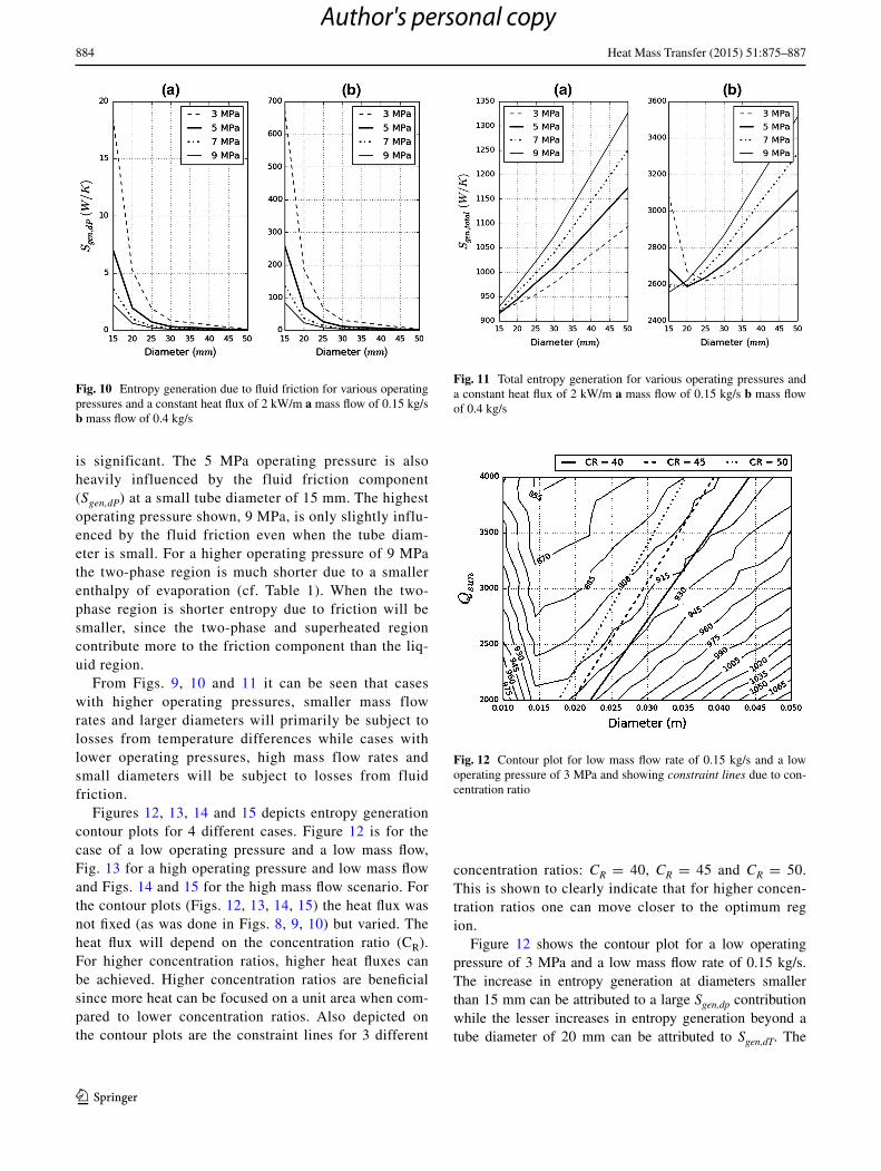
Figure 10 shows the change in entropy generation due to fluid friction for different cases. Figure 10a is for a low mass flow case whereas Fig. 10b is for a high mass flow case. Smaller diameters will significantly increase the entropy due to friction. This is especially true for the higher mass flow case and low operating pressure. Increas-ing the operating pressure will have the effect of lowering the entropy generation due to friction. This is due to the shorter two-phase regions for higher operating pressures as well as smaller pressure drops in the superheated region (due to higher vapour densities). The liquid regions are often longer for higher operating pressures but the entropy generation due to fluid friction in this region is small when compared to the other regions. Decreasing the diameter has the effect of quadratically increasing the entropy generation due to friction.

Figure 11 depicts the total entropy generation (com-bined Sgen,dT and Sgen,dP). It can be seen from Fig. 11a (for a low mass flow case) that the entropy generation due to friction has a slight influence on the lowest oper-ating pressure, 3 MPa. The influence of fluid friction is seen more readily in Fig. 11b which is for the high mass flow case. For a high mass flow case the 3 MPa operating pressure is highly influenced by Sgen,dP at diameters 15 and 20 mm. The reason for a total entropy generation above 3,000 W/K for the 15 mm case is that even though the heat losses are small the fluid friction

Fig. 7 Heat transfer coefficient for the two-phase region for the case of Tsat = 250.4 °C (4 MPa), Di = 25 mm, Qsun = 2 kW/m and a mass flow of 0.2 kg/s

Fig. 8 Glass, fluid and receiver temperature for the two-phase region for the case of Tsat = 250.4 °C (4 MPa), Di = 25 mm, Qsun = 2 kW/m and a mass flow of 0.2 kg/s

Fig. 9 Entropy generation due to finite temperature differences for various operating pressures and a constant heat flux of 2 kW/m a mass flow of 0.15 kg/s b mass flow of 0.4 kg/s

Author's personal copy

884 Heat Mass Transfer (2015) 51:875–887

1 3

is significant. The 5 MPa operating pressure is also heavily influenced by the fluid friction component (Sgen,dP) at a small tube diameter of 15 mm. The highest operating pressure shown, 9 MPa, is only slightly influ-enced by the fluid friction even when the tube diam-eter is small. For a higher operating pressure of 9 MPa the two-phase region is much shorter due to a smaller enthalpy of evaporation (cf. Table 1). When the two-phase region is shorter entropy due to friction will be smaller, since the two-phase and superheated region contribute more to the friction component than the liq-uid region.

From Figs. 9, 10 and 11 it can be seen that cases with higher operating pressures, smaller mass flow rates and larger diameters will primarily be subject to losses from temperature differences while cases with lower operating pressures, high mass flow rates and small diameters will be subject to losses from fluid friction.

Figures 12, 13, 14 and 15 depicts entropy generation contour plots for 4 different cases. Figure 12 is for the case of a low operating pressure and a low mass flow, Fig. 13 for a high operating pressure and low mass flow and Figs. 14 and 15 for the high mass flow scenario. For the contour plots (Figs. 12, 13, 14, 15) the heat flux was not fixed (as was done in Figs. 8, 9, 10) but varied. The heat flux will depend on the concentration ratio (CR). For higher concentration ratios, higher heat fluxes can be achieved. Higher concentration ratios are beneficial since more heat can be focused on a unit area when com-pared to lower concentration ratios. Also depicted on the contour plots are the constraint lines for 3 different

concentration ratios: CR = 40, CR = 45 and CR = 50. This is shown to clearly indicate that for higher concen-tration ratios one can move closer to the optimum region.

Figure 12 shows the contour plot for a low operating pressure of 3 MPa and a low mass flow rate of 0.15 kg/s. The increase in entropy generation at diameters smaller than 15 mm can be attributed to a large Sgen,dp contribution while the lesser increases in entropy generation beyond a tube diameter of 20 mm can be attributed to Sgen,dT. The

Fig. 10 Entropy generation due to fluid friction for various operating pressures and a constant heat flux of 2 kW/m a mass flow of 0.15 kg/s b mass flow of 0.4 kg/s

Fig. 11 Total entropy generation for various operating pressures and a constant heat flux of 2 kW/m a mass flow of 0.15 kg/s b mass flow of 0.4 kg/s

Fig. 12 Contour plot for low mass flow rate of 0.15 kg/s and a low operating pressure of 3 MPa and showing constraint lines due to con-centration ratio

Author's personal copy

885Heat Mass Transfer (2015) 51:875–887

1 3

feasible region is located below the constraint lines to the right and can be represented as follows for a concentration ratio of 45:

From Fig. 12 it can be seen that diameters smaller than 15 mm tend to be highly influenced by Sgen,dp. This is due to the fluid friction component being more prevalent for smaller diameters. The optimum is located at the upper left region where Qsun is at a maximum and the diameter

(26a)CR ≤ 45

(26b)g(X)− 45 ≤ 0

remains small (but larger than 15 mm) to minimize losses to ambient. Beyond 20 mm the total entropy generation is mostly influenced by Sgen,dT. Increasing the diameter as well as the maximum amount of focused heat per unit section (Qsun), will always have the effect of decreasing the entropy generation. This is due to the constraint lines having a steeper gradient than the contour plot lines that signify the Sgen,dT contribution. It is however impractical to increase the receiver diameter and concentration ratio indefinitely simply to decrease the entropy generation. When taking the constraint into account, good design choices are located at Di = 20 mm and Qsun ≈ 2 kW/m. Larger diameters such as 35 mm will require a Qsun of around 3.5 kW/m.

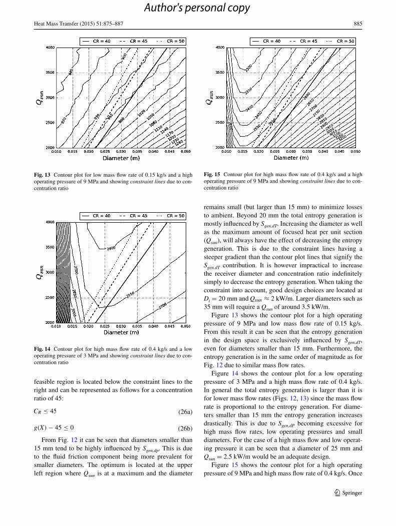
Figure 13 shows the contour plot for a high operating pressure of 9 MPa and low mass flow rate of 0.15 kg/s. From this result it can be seen that the entropy generation in the design space is exclusively influenced by Sgen,dT, even for diameters smaller than 15 mm. Furthermore, the entropy generation is in the same order of magnitude as for Fig. 12 due to similar mass flow rates.

Figure 14 shows the contour plot for a low operating pressure of 3 MPa and a high mass flow rate of 0.4 kg/s. In general the total entropy generation is larger than it is for lower mass flow rates (Figs. 12, 13) since the mass flow rate is proportional to the entropy generation. For diame-ters smaller than 15 mm the entropy generation increases drastically. This is due to Sgen,dP becoming excessive for high mass flow rates, low operating pressures and small diameters. For the case of a high mass flow and low operat-ing pressure it can be seen that a diameter of 25 mm and Qsun = 2.5 kW/m would be an adequate design.

Figure 15 shows the contour plot for a high operating pressure of 9 MPa and high mass flow rate of 0.4 kg/s. Once

Fig. 13 Contour plot for low mass flow rate of 0.15 kg/s and a high operating pressure of 9 MPa and showing constraint lines due to con-centration ratio

Fig. 14 Contour plot for high mass flow rate of 0.4 kg/s and a low operating pressure of 3 MPa and showing constraint lines due to con-centration ratio

Fig. 15 Contour plot for high mass flow rate of 0.4 kg/s and a high operating pressure of 9 MPa and showing constraint lines due to con-centration ratio

Author's personal copy

886 Heat Mass Transfer (2015) 51:875–887

1 3

again (if the constraint is ignored) the optimum region is located in the upper left region were the inner tube diam-eter (Di) is fairly small (15 mm) and Qsun is at a maximum. When comparing Fig. 14 (for a low operating pressure) and Fig. 15 (for a high operating pressure) it can be seen that Sgen,dT tends to be more dominant for the higher operating pressure. When increasing the diameter beyond 20 mm for an operating condition of 9 MPa the increase in Sgen,dT is more significant than for 3 MPa. This is due to the Sgen,dT component having a larger impact on the total entropy gen-eration at high saturation temperatures. However, decreas-ing Di beyond 15 mm (in the case of an operating pressure of 3 MPa) will increase the entropy generation drastically. This is due to the Sgen,dp component becoming excessive for lower operating pressures, partly due to the longer two-phase regions as well as a larger two-phase flow multiplier for the lower operating pressures.

The simulated annealing results are shown in Table 4. The optimal operating pressure increases as the mass flow rate increases. It should however, also be recognised that higher mass flow rates will result in more available work. Ideally one would like a high work output, while still achieving low entropy generation rates.

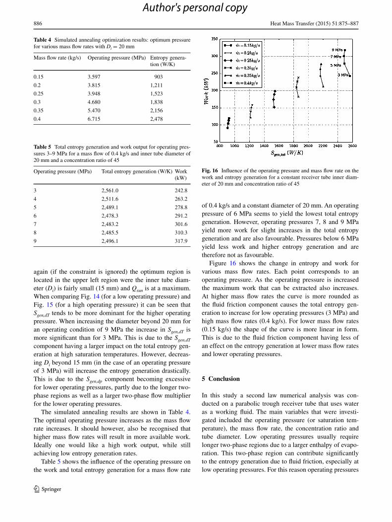
Table 5 shows the influence of the operating pressure on the work and total entropy generation for a mass flow rate

of 0.4 kg/s and a constant diameter of 20 mm. An operating pressure of 6 MPa seems to yield the lowest total entropy generation. However, operating pressures 7, 8 and 9 MPa yield more work for slight increases in the total entropy generation and are also favourable. Pressures below 6 MPa yield less work and higher entropy generation and are therefore not as favourable.

Figure 16 shows the change in entropy and work for various mass flow rates. Each point corresponds to an operating pressure. As the operating pressure is increased the maximum work that can be extracted also increases. At higher mass flow rates the curve is more rounded as the fluid friction component causes the total entropy gen-eration to increase for low operating pressures (3 MPa) and high mass flow rates (0.4 kg/s). For lower mass flow rates (0.15 kg/s) the shape of the curve is more linear in form. This is due to the fluid friction component having less of an effect on the entropy generation at lower mass flow rates and lower operating pressures.

5 Conclusion

In this study a second law numerical analysis was con-ducted on a parabolic trough receiver tube that uses water as a working fluid. The main variables that were investi-gated included the operating pressure (or saturation tem-perature), the mass flow rate, the concentration ratio and tube diameter. Low operating pressures usually require longer two-phase regions due to a larger enthalpy of evapo-ration. This two-phase region can contribute significantly to the entropy generation due to fluid friction, especially at low operating pressures. For this reason operating pressures

Table 4 Simulated annealing optimization results: optimum pressure for various mass flow rates with Di = 20 mm

Mass flow rate (kg/s) Operating pressure (MPa) Entropy genera-tion (W/K)

0.15 3.597 903

0.2 3.815 1,211

0.25 3.948 1,523

0.3 4.680 1,838

0.35 5.470 2,156

0.4 6.715 2,478

Table 5 Total entropy generation and work output for operating pres-sures 3–9 MPa for a mass flow of 0.4 kg/s and inner tube diameter of 20 mm and a concentration ratio of 45

Operating pressure (MPa) Total entropy generation (W/K) Work (kW)

3 2,561.0 242.8

4 2,511.6 263.2

5 2,489.1 278.8

6 2,478.3 291.2

7 2,483.2 301.6

8 2,485.5 310.3

9 2,496.1 317.9

Fig. 16 Influence of the operating pressure and mass flow rate on the work and entropy generation for a constant receiver tube inner diam-eter of 20 mm and concentration ratio of 45

Author's personal copy

887Heat Mass Transfer (2015) 51:875–887

1 3

below 3 MPa are not recommended regardless of mass flow rate or receiver tube diameter.

Contributions from the entropy fluid friction compo-nent can be extreme for high mass flow rates and diameters smaller than 15 mm. In general, the fluid friction com-ponent becomes small when compared to the finite tem-perature difference component, for diameters larger than 20 mm. Increasing the receiver tube diameter will increase the entropy due to temperature differences if the maximum amount of focused heat (Qsun) is kept constant. This is due to the increased exposed heat transfer surface. The heat flux (Qsun) is determined by the concentration ratio and is lim-ited to around 45 for 2D trough technology. On the other hand increasing receiver tube diameter as well as Qsun will decrease the entropy generation, but this effect is only mar-ginal for larger tube diameters.

It was also seen that the optimal operating pressure tends to increase if higher mass flow rates are considered. Higher operating pressures tend to have a more advantageous effect on the maximum work output while having a small to negligible effect on increasing the entropy generation.

Acknowledgments We would like to thank the University of Pre-toria, University of Stellenbosch, NRF, TESP, SANERI/SANEDI, CSIR, EEDSM hub and NAC for the funding during the course of this work.

References

1. Eck M, Zarza E, Eickhoff M, Rheinländer J, Valenzuela L (2003) Applied research concerning the direct steam generation in para-bolic troughs. Sol Energy 74:341–351

2. Price H, Lüpfert E, Kearney D, Zarza E, Cohen G, Gee R, Mohoney R (2002) Advances in parabolic trough solar technol-ogy. J Sol Energy Eng 124:109–125

3. Liu QB, Wang YL, Gao ZC, Sui J, Jin HG, Li HP (2010) Experi-mental investigation on a parabolic trough solar collector for ther-mal power generation. Sci China Tech Sci 53:52–56

4. Odeh S, Morrison G, Behnia M (1998) Modelling of parabolic trough direct steam generation solar collectors. Sol Energy 62:395–406

5. Forristall R (2003) Heat transfer analysis and modelling of a par-abolic trough solar receiver implemented in engineering equation solver. Technical Report; National Renewable Energy Laboratory

6. Roesle M, Coskun V, Steinfeld A (2011) Numerical analysis of heat loss from a parabolic trough absorber tube with active vac-uum system. J Sol Eng 133:1–5

7. Koroneos C, Spachos T, Moussiopoulos N (2003) Exergetic anal-ysis of renewable energy sources. Renew Energy 28:295–310

8. Singh N, Kanshik S, Misra R (2000) Exergetic analysis of a solar thermal power systems. Renew Energy 19:135–143

9. Bejan A (1996) Entropy generation minimization: the method of thermodynamic optimization of finite size systems and finite time processes. CRC Press, Boca Raton

10. Ratts E, Raut A (2004) Entropy generation minimisation of fully developed internal flow with constant heat flux. J Heat Transf 126:656–659

11. Sahin A (2000) Entropy generation in turbulent liquid flow through a smooth duct subjected to constant wall temperature. Int J Heat Mass Transf 43:1469–1478

12. Revellin R, Lips S, Khandehar S, Bonjour J (2009) Local entropy generation for saturated two-phase flow. Energy 34:1113–1121

13. Barlev D, Vidu R, Stroewe P (2011) Innovations in concentrated solar power. Sol Energy Mat Sol Cells 95(27):3–25

14. Gnielinsky V (1976) New equations for heat and mass transfer in turbulent pipe and channel flow. Int Chem Eng 1(2):350–367

15. Petukhov B (1970) Heat transfer and friction in turbulent pipe flow with variable physical properties. Adv Heat Transf 6:503–564

16. Wojtan L, Ursenbacher T, Thome J (2005) Investigation of flow boiling in horizontal tubes part 1: a new diabetic two-phase flow pattern map. Int J Heat Mass Transf 48:2955–2969

17. Wojtan L, Ursenbacher T, Thome J (2005) Investigation of flow boiling in horizontal tubes part 2: development of a new heat transfer model for stratified-wavy, dryout and misty flow regimes. Int J Heat Mass Transf 48:2970–2985

18. Kattan N, Thome JR, Favrat D (1998) Flow boiling in horizontal tubes: part 1—development of a diabatic two-phase flow pattern map. J Heat Transf 120:140–147

19. Zürcher O, Favrat D, Thome JR (2002) Evaporation of refrig-erants in a horizontal tube: an improved flow patter dependent heat transfer model compared to ammonia data. Int J Heat Mass Transf 45:303–317

20. Churchill S, Bernstein M (1977) A correlating equation for forced convection from gases and liquids to a circular cylinder in cross-flow. J Heat Transf T ASME C 99:300–306

21. Kalogirou S (2009) Solar energy engineering: processes and sys-tems. Elsevier, Amsterdam

22. Garcia-Valladares O, Velázquez N (2009) Numerical simula-tion of parabolic trough collector: improvement using counter-flow concentric circular heat exchangers. J Heat Mass Transf 52:597–609

23. Thome J (2004) Wolverine tube heat transfer data book III. Wol-verine Tube Inc. http://www.wlv.com

24. Friedel F (1979) Improved friction pressure drop correlations for horizontal and vertical two-phase pipe flow. European two-phase flow group meeting, Ispra, Italy, Paper E2

25. Coolprop BI (2013) http://coolprop-sourceforge.net 26. Python Software Foundation. Python (2011) http://www.

python.org/doc/ 27. Scipy Community. Scipy (2011) http://docs.scipy.org/doc/

Author's personal copy