Archvied in

http://dspace.nitrkl.ac.in/dspace

Published in Computers & Chemical Engineering (accepted)

http://dx.doi.org/10.1016/j.compchemeng.2007.10.012

Selection of optimal feed flow sequence for a multiple effect evaporator

system

R. Bhargavaa, S. Khanamb,*, B. Mohantya and A. K. Rayc

a Department of Chemical Engineering, Indian Institute of Technology Roorkee,

Roorkee – 247 667, India

b Department of Chemical Engineering, National Institute of Technology Rourkela,

Rourkela – 769 008, India

c Department of Paper Technology, Indian Institute of Technology Roorkee,

Roorkee – 247 667, India

Abstract

A nonlinear model is developed for a SEFFFE system employed for concentrating weak

black liquor in an Indian Kraft Paper Mill. The system incorporates different operating

strategies such as condensate-, feed- & product- flashing and steam- & feed- splitting. This

model is capable of simulating a MEE system by accounting variations in τ, U, Qloss, physico-

thermal properties of the liquor, F and operating strategies.

The developed model is used to analyze six different F including backward as well as mixed

flow sequences. For these F, the effects of variations of input parameters, T0 and F, on output

parameters such as SC and SE have been studied to select the optimal F for the complete

range of operating parameters. Thus, this model is used as a screening tool for the selection of

an optimal F amongst the different F.

An advantage of the present model is that a F is represented using an input Boolean matrix

and to change the F this input matrix needs to be changed rather than modifying the complete

set of model equations for each F. It is found that for the SEFFFE system, backward feed

flow sequence is the best as far as SE is concerned.

Keywords: Screening tool, Optimal feed flow sequence, Flat falling film Evaporator system,

Steam economy

1. Introduction

An energy audit shows that MEE House of an Indian Paper industry consumes about 24-30 %

of its total energy (Rao and Kumar, 1985) and thus any measure to cut down this taxing

energy bill by proper selection of operational strategy will improve the profitability of the

plant. Keeping this fact in mind, since last few decades researchers have tried to develop

* Corresponding author: E-mail address: shabinahai@gmail.com, skhanam@nitrkl.ac.in Phone No. +91-9938185505, +91-661-2464251

operating strategies for MEE systems, which would consume minimum amount of live steam

and in other words would provide maximum SE to the system. These operating strategies

include flow sequences of feed for operation, feed-, product- & condensate- flashing and

feed- & steam- splitting. However, one of the easiest ways to increase SE of the system is to

operate the MEE system with optimal F. However, screening the optimal F, out of the

feasible ones, is time consuming and if done experimentally becomes an arduous task. One

reasonable way of doing it is to use simulation.

For the analysis of MEE system many investigators have proposed mathematical models. A

few of these were developed by Kern (1950), Itahara and Stiel (1966), Holland (1975),

Radovic et al. (1979), Lambert et al. (1987), Mathur (1992), Bremford and Muller-

Steinhagen (1994), El-Dessouky et al. (1998, 2000) and Bhargava (2004). These models were

not used for the selection of optimal F. However, for this purpose Harpor and Tsao (1972)

developed a model for the optimization of a MEE system considering forward- and

backward- F. Their work was extended by Nishitani and Kunugita (1979) to propose an

algorithm for generating non-inferior F amongst all possible F of a MEE system. The non-

inferior F were based on the constraints of viscosity of liquid and the formation of scale

and/or foam. They suggested that if an optimal F is required, one should examine the set of

non-inferior F.

All these mathematical models are generally based on a set of linear/nonlinear equations and

accommodate effects of varying physical properties of vapor/steam and liquor with

temperature. These models either use fixed value of U for different effects or variable U

based on empirical equations or mathematical models.

It is a fact that set of model equations developed for a given operating strategy does not work

when the strategy is changed. In fact, it compels one to restructure and reformulate the whole

set of governing equations to address the new operating strategy. For example, if operating

strategy such as flow sequences, liquor splitting and conditions of flashing is changed, the

governing equations, which describe this operating strategy must be changed (Mathur, 1992).

The above fact further adds difficulty in simulating all the operating strategies through a

given model without changing the set of its governing equations. On the other hand Stewart

and Beveridge (1977) and Ayangbile et al. (1984) developed generalized cascade algorithm

in which the model of an evaporator body is solved repeatedly to address the different

operating strategies of a MEE system. With the change in operating strategy the sequence of

the solution of the model equation of the effect and the input data to it changes. The solution

strategy, employed for solving the model, automatically selects the above sequence based on

the input data file where the investigator describes the operating strategy.

The modeling technique proposed by Ayangbile et al. (1984) has been further modified and

improved in the present work to account for feed sequencing, feed- & steam- splitting and

condensate-, feed- and product- flashing. Besides the above, the improved model also

considers variations in τ, U, Qloss from surfaces of different effects and physico-thermal

properties of steam/vapor, condensate and liquor, which were not accounted in the work of

Ayangbile et al. (1987). This model is used as a screening tool for the selection of optimal F

for a MEE system.

2. Problem statement

The MEE system selected for above investigation is a SEFFFE system that is being operated

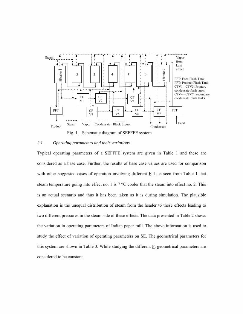
in a nearby Indian Kraft Paper Mill for concentrating weak black liquor. The schematic

diagram of a SEFFFE system with backward F is shown in Fig. 1. The first two effects of it

are considered as finishing effects, which require live steam and the seventh effect is attached

to a vacuum unit. This system employs feed- & steam- splitting, feed- and product-flashing

along with primary and secondary condensate flashing to generate auxiliary vapor, which are

then used in vapor bodies of appropriate effects to improve overall SE of the system.

2.1. Operating parameters and their variations

Typical operating parameters of a SEFFFE system are given in Table 1 and these are

considered as a base case. Further, the results of base case values are used for comparison

with other suggested cases of operation involving different F. It is seen from Table 1 that

steam temperature going into effect no. 1 is 7 °C cooler that the steam into effect no. 2. This

is an actual scenario and thus it has been taken as it is during simulation. The plausible

explanation is the unequal distribution of steam from the header to these effects leading to

two different pressures in the steam side of these effects. The data presented in Table 2 shows

the variation in operating parameters of Indian paper mill. The above information is used to

study the effect of variation of operating parameters on SE. The geometrical parameters for

this system are shown in Table 3. While studying the different F, geometrical parameters are

considered to be constant.

Steam

FFT: Feed Flash Tank PFT: Product Flash Tank CFV1 - CFV3: Primary condensate flash tanks CFV4 - CFV7: Secondary condensate flash tanks

Feed

Effec

t No 1

2

3

4

5

6

Effec

t No 7

CFV1

CFV2

CFV3

CFV7

CFV6

CFV5

CFV4

FFT

Condensate

Vapor from Last effect

Steam Vapor Condensate Black Liquor

Fig. 1. Schematic diagram of SEFFFE system Product

PFT

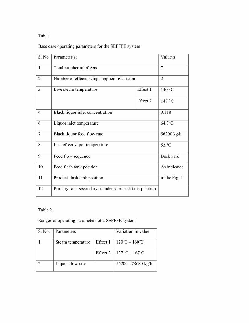
Table 1

Base case operating parameters for the SEFFFE system

S. No Parameter(s) Value(s)

1 Total number of effects 7

2 Number of effects being supplied live steam 2

3 Live steam temperature Effect 1 140 °C

Effect 2 147 °C

4 Black liquor inlet concentration 0.118

6 Liquor inlet temperature 64.7oC

7 Black liquor feed flow rate 56200 kg/h

8 Last effect vapor temperature 52 °C

9 Feed flow sequence Backward

10 Feed flash tank position As indicated

in the Fig. 1 11 Product flash tank position

12 Primary- and secondary- condensate flash tank position

Table 2

Ranges of operating parameters of a SEFFFE system

S. No. Parameters Variation in value

1. Steam temperature Effect 1 120oC – 160oC

Effect 2 127 oC – 167oC

2. Liquor flow rate 56200 - 78680 kg/h

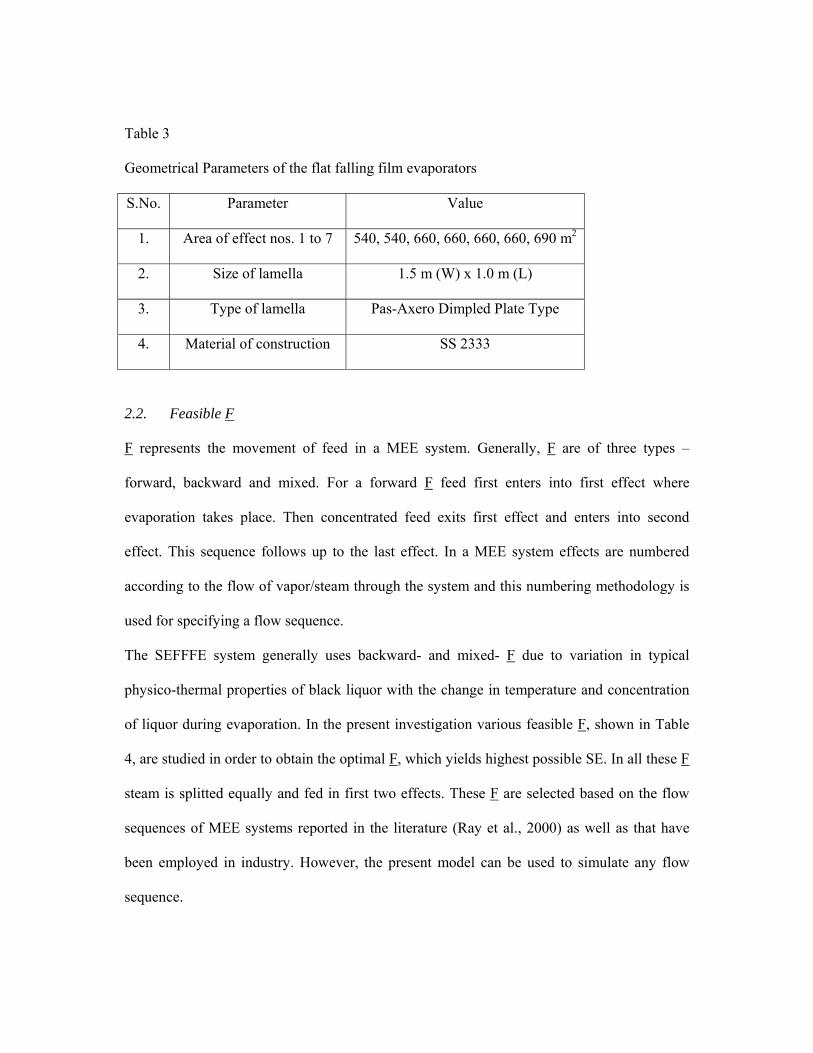
Table 3

Geometrical Parameters of the flat falling film evaporators

S.No. Parameter Value

1. Area of effect nos. 1 to 7 540, 540, 660, 660, 660, 660, 690 m2

2. Size of lamella 1.5 m (W) x 1.0 m (L)

3. Type of lamella Pas-Axero Dimpled Plate Type

4. Material of construction SS 2333

2.2. Feasible F

F represents the movement of feed in a MEE system. Generally, F are of three types –

forward, backward and mixed. For a forward F feed first enters into first effect where

evaporation takes place. Then concentrated feed exits first effect and enters into second

effect. This sequence follows up to the last effect. In a MEE system effects are numbered

according to the flow of vapor/steam through the system and this numbering methodology is

used for specifying a flow sequence.

The SEFFFE system generally uses backward- and mixed- F due to variation in typical

physico-thermal properties of black liquor with the change in temperature and concentration

of liquor during evaporation. In the present investigation various feasible F, shown in Table

4, are studied in order to obtain the optimal F, which yields highest possible SE. In all these F

steam is splitted equally and fed in first two effects. These F are selected based on the flow

sequences of MEE systems reported in the literature (Ray et al., 2000) as well as that have

been employed in industry. However, the present model can be used to simulate any flow

sequence.

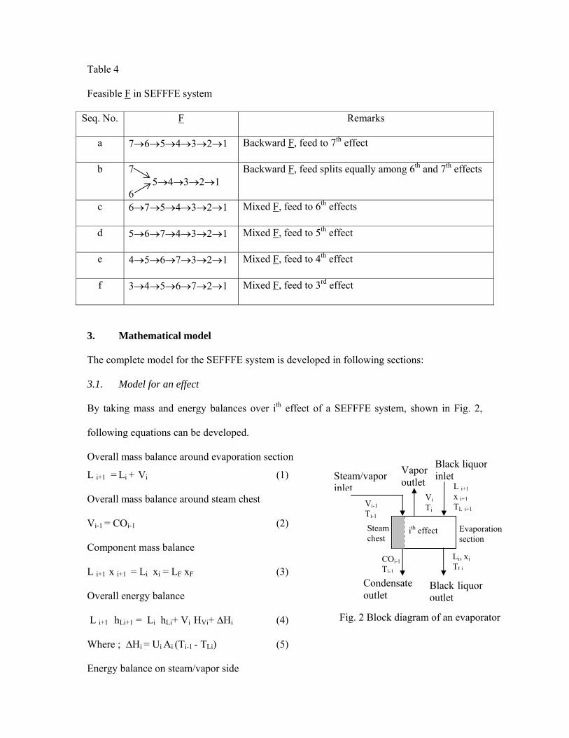
Table 4

Feasible F in SEFFFE system

Seq. No. F Remarks

a 7→6→5→4→3→2→1 Backward F, feed to 7th effect

b 7 5→4→3→2→1 6

Backward F, feed splits equally among 6th and 7th effects

c 6→7→5→4→3→2→1 Mixed F, feed to 6th effects

d 5→6→7→4→3→2→1 Mixed F, feed to 5th effect

e 4→5→6→7→3→2→1 Mixed F, feed to 4th effect

f 3→4→5→6→7→2→1 Mixed F, feed to 3rd effect

3. Mathematical model

The complete model for the SEFFFE system is developed in following sections:

3.1. Model for an effect

By taking mass and energy balances over ith effect of a SEFFFE system, shown in Fig. 2,

following equations can be developed.

Overall mass balance around evaporation section

L i+1 = Li + Vi (1)

Overall mass balance around steam chest

Vi-1 = COi-1 (2)

Component mass balance

L i+1 x i+1 = Li xi = LF xF (3)

Overall energy balance

L i+1 hLi+1 = Li hLi+ Vi HVi+ ∆Hi (4)

Where ; ∆Hi = Ui Ai (Ti-1 - TLi) (5)

Energy balance on steam/vapor side

Steam/vapor inlet

Vapor outlet

Vi Ti

Black liquor inlet

L i+1 x i+1 TL i+1 Vi-1

Ti-1

Li, xi TLi

COi-1 Ti-1

Condensate outlet

Black liquor outlet

Fig. 2 Block diagram of an evaporator

ith effect Steam chest

Evaporation section

Vi-1 = ∆Hi / (HVi-1 - hLi-1) (6)

The correlations for enthalpy (hL) for black liquor is given as:

hL = CPP* (TL – C5) J/ kg (7)

where, CPP = C1 * (1-C4x) and TL = T + τ

The values of coefficients C1, C4 and C5, used in Eq. 7, are 4187, 0.54 and 273, respectively.

For the development of a correlation for τ of black liquor, the functional relationship is taken

from well established TAPPI correlation (Ray et al., 1992). For ith effect where concentration

of black liquor is xi, τ is given as:

τi = C3 (C2 +xi)2 (8)

The correlation of τ is obtained by fitting Eq. 8 against the data of a nearby paper mill as

given in Table 5. The value of C3 is computed as 20, using value of C2 as 0.1 (Ray et al.,

1992). This correlation gives a maximum error of 6% with an average error of 3.4%.

Table 5

Data for the determination of τ

xi 0.0767 0.091 0.106 0.13 0.169 0.244 0.369 0.462 0.47

τi ,K 0.60 0.70 0.80 1.10 1.40 2.30 4.30 6.20 6.40

Combining Eqs. 1 to 8 and eliminating Vi , xi, hi, ∆Hi and TLi one gets following cubic

polynomial in terms of Li:

a1 Li 3 + a2 Li

2 +a3 Li + a4 = 0 (9)

where coefficients a1, a2, a3 and a4 are functions of input liquor parameters and other known

parameters like heat transfer area (Ai) and overall heat transfer coefficient (Ui) of the effect

for which it is being used.

The expression for coefficients a1, a2, a3 and a4 are:

a1 = HVi –C1Ti – C1C22C3 + C1C5 (9a)

a2 = Li+1 hLi+1 + UiAi (Ti-1 – Ti – C3C22) + Li+1 xi+1 (C1C4Ti -2C1C2C3 + C1C3C2

2C4 – C1C4C5

– Li+1 HVi) (9b)

a3 = (Li+1 xi+1)2 (2C1C2 C3C4 - C1C3 ) - 2C2C3 Ui Ai Li+1 xi+1 (9c)

and a4 = (C1C3C4 Li+1 xi+1 - C3 Ui Ai) (Li+1 xi+1)2 (9d)

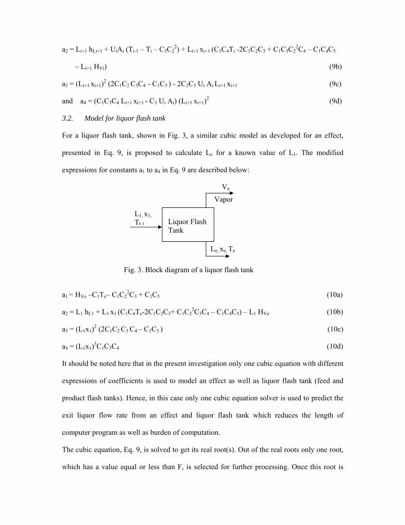
3.2. Model for liquor flash tank

For a liquor flash tank, shown in Fig. 3, a similar cubic model as developed for an effect,

presented in Eq. 9, is proposed to calculate Le for a known value of L1. The modified

expressions for constants a1 to a4 in Eq. 9 are described below:

a1 = HVe –C1Te– C1C22C3 + C1C5 (10a)

a2 = L1 hL1 + L1 x1 (C1C4Te-2C1C2C3+ C1C22C3C4 – C1C4C5) – L1 HVe (10b)

a3 = (L1x1)2 (2C1C2 C3 C4 – C1C3 ) (10c)

a4 = (L1x1)3C1C3C4 (10d)

It should be noted here that in the present investigation only one cubic equation with different

expressions of coefficients is used to model an effect as well as liquor flash tank (feed and

product flash tanks). Hence, in this case only one cubic equation solver is used to predict the

exit liquor flow rate from an effect and liquor flash tank which reduces the length of

computer program as well as burden of computation.

The cubic equation, Eq. 9, is solved to get its real root(s). Out of the real roots only one root,

which has a value equal or less than F, is selected for further processing. Once this root is

Vapor

L1, x1, TL1

Le, xe, Te

Liquor Flash Tank

Fig. 3. Block diagram of a liquor flash tank

Ve

known, other parameters like exit liquor -concentration, -temperature, vapor produced (Vi)

and the quantity of vapor required (Vi-1) are computed using Eqs. 3, 4, 1 & 6, respectively.

3.3. Model for condensate flash tank

Material and energy balances over condensate flash tank yields following relation to

determine exit condensate flow rate (COj), for a known condensate mass flow rate, COi,

entering at a temperature, Ti, with specific enthalpy, hi, and being flashed at temperature, Tj

to generate vapor of amount, Vj. The overall mass and energy balance give:

COj = COi (Hvj - hi)/ (Hvj - hj) (11)

and Vj = COi - COj (12)

3.4. Empirical correlations for U and Qloss

The present model for a SEFFFE system uses empirical correlations for the prediction of U

and Qloss from each effect. For development of these empirical correlations the data is

collected from a Indian Kraft Paper Mill employing SEFFFE system.

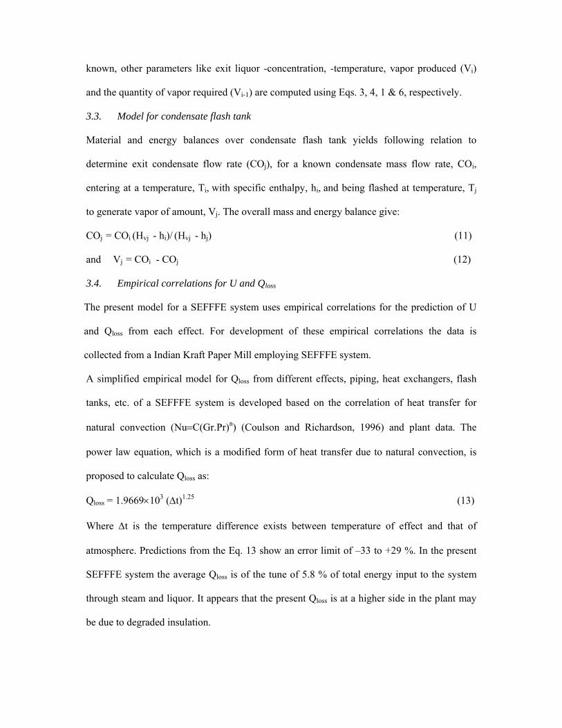
A simplified empirical model for Qloss from different effects, piping, heat exchangers, flash

tanks, etc. of a SEFFFE system is developed based on the correlation of heat transfer for

natural convection (Nu=C(Gr.Pr)n) (Coulson and Richardson, 1996) and plant data. The

power law equation, which is a modified form of heat transfer due to natural convection, is

proposed to calculate Qloss as:

Qloss = 1.9669×103 (Δt)1.25 (13)

Where Δt is the temperature difference exists between temperature of effect and that of

atmosphere. Predictions from the Eq. 13 show an error limit of –33 to +29 %. In the present

SEFFFE system the average Qloss is of the tune of 5.8 % of total energy input to the system

through steam and liquor. It appears that the present Qloss is at a higher side in the plant may

be due to degraded insulation.

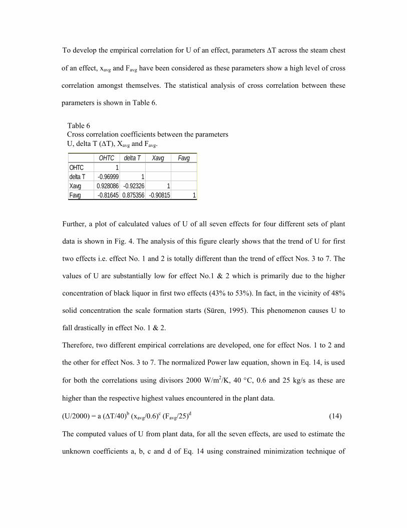
To develop the empirical correlation for U of an effect, parameters ΔT across the steam chest

of an effect, xavg and Favg have been considered as these parameters show a high level of cross

correlation amongst themselves. The statistical analysis of cross correlation between these

parameters is shown in Table 6.

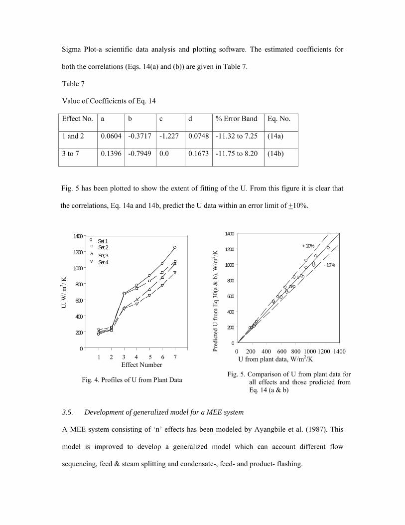
Further, a plot of calculated values of U of all seven effects for four different sets of plant

data is shown in Fig. 4. The analysis of this figure clearly shows that the trend of U for first

two effects i.e. effect No. 1 and 2 is totally different than the trend of effect Nos. 3 to 7. The

values of U are substantially low for effect No.1 & 2 which is primarily due to the higher

concentration of black liquor in first two effects (43% to 53%). In fact, in the vicinity of 48%

solid concentration the scale formation starts (Süren, 1995). This phenomenon causes U to

fall drastically in effect No. 1 & 2.

Therefore, two different empirical correlations are developed, one for effect Nos. 1 to 2 and

the other for effect Nos. 3 to 7. The normalized Power law equation, shown in Eq. 14, is used

for both the correlations using divisors 2000 W/m2/K, 40 °C, 0.6 and 25 kg/s as these are

higher than the respective highest values encountered in the plant data.

(U/2000) = a (ΔT/40)b (xavg/0.6)c (Favg/25)d (14)

The computed values of U from plant data, for all the seven effects, are used to estimate the

unknown coefficients a, b, c and d of Eq. 14 using constrained minimization technique of

OHTC delta T Xavg FavgOHTC 1delta T -0.96999 1Xavg 0.928086 -0.92326 1Favg -0.81645 0.875356 -0.90815 1

Table 6 Cross correlation coefficients between the parameters U, delta T (ΔT), Xavg and Favg.

Sigma Plot-a scientific data analysis and plotting software. The estimated coefficients for

both the correlations (Eqs. 14(a) and (b)) are given in Table 7.

Table 7

Value of Coefficients of Eq. 14

Effect No. a b c d % Error Band Eq. No.

1 and 2 0.0604 -0.3717 -1.227 0.0748 -11.32 to 7.25 (14a)

3 to 7 0.1396 -0.7949 0.0 0.1673 -11.75 to 8.20 (14b)

Fig. 5 has been plotted to show the extent of fitting of the U. From this figure it is clear that

the correlations, Eq. 14a and 14b, predict the U data within an error limit of +10%.

3.5. Development of generalized model for a MEE system

A MEE system consisting of ‘n’ effects has been modeled by Ayangbile et al. (1987). This

model is improved to develop a generalized model which can account different flow

sequencing, feed & steam splitting and condensate-, feed- and product- flashing.

F i g . 5 . 1 P r o f i l e s o f O H T C f r o m P l a ntDataE f f e c t N o .

0 1 2 3 4 5 6 7 8

fr

lntaa//

0

2 0 0

4 0 0

6 0 0

8 0 0

1 0 0 0

1 2 0 0

1 4 0 0 S e t 1 S e t 2 S e t 3 S e t 4

U, W

/ m2 / K

1 2 3 4 5 6 7 Effect Number Fig. 4. Profiles of U from Plant Data

0 200 400 600 8 0 0 1 0 0 0 1 2 00 1400

PredictedValuesofOHTCW/sqm/K

0

200

400

600

800

1000

1200

1400

- 10%

+ 1 0 %

Pred

icte

d U

from

Eq

30(a

& b

), W

/m2 /K

0 200 400 600 800 1000 1200 1400 U from plant data, W/m2/K Fig. 5. Comparison of U from plant data for

all effects and those predicted from Eq. 14 (a & b)

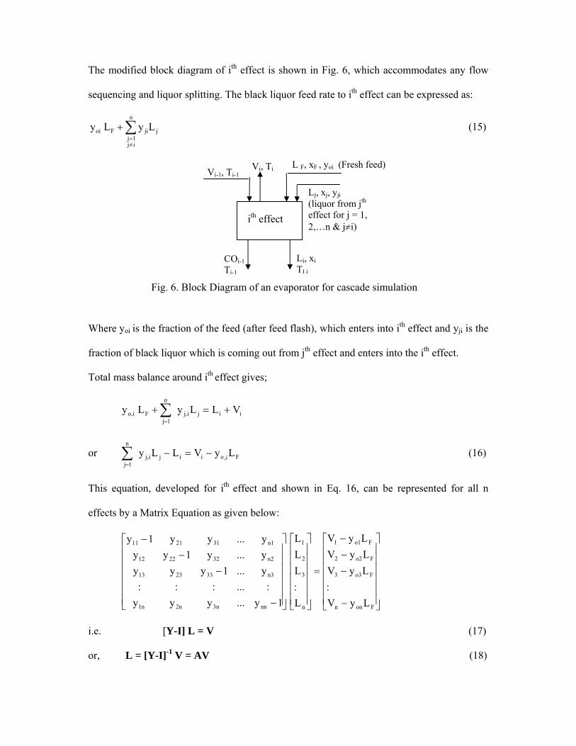
The modified block diagram of ith effect is shown in Fig. 6, which accommodates any flow

sequencing and liquor splitting. The black liquor feed rate to ith effect can be expressed as:

∑≠=

+n

ij1j

jjiFoi LyL y (15)

Where yoi is the fraction of the feed (after feed flash), which enters into ith effect and yji is the

fraction of black liquor which is coming out from jth effect and enters into the ith effect.

Total mass balance around ith effect gives;

iijj,i1j

Fo,i VLLy Ly +=+ ∑=

n

or F,ioiijj,i

n

1j

LyVLLy −=−∑=

(16)

This equation, developed for ith effect and shown in Eq. 16, can be represented for all n

effects by a Matrix Equation as given below:

⎥⎥⎥⎥⎥⎥

⎦

⎤

⎢⎢⎢⎢⎢⎢

⎣

⎡

−

−−−

=

⎥⎥⎥⎥⎥⎥

⎦

⎤

⎢⎢⎢⎢⎢⎢

⎣

⎡

⎥⎥⎥⎥⎥⎥

⎦

⎤

⎢⎢⎢⎢⎢⎢

⎣

⎡

−

−−

−

Fonn

Fo33

Fo22

Fo11

n

3

2

1

nn3n2n1n

n3332313

n2322212

n1312111

LyV:

LyVLyVLyV

L:LLL

1y...yyy:...:::

y...1yyyy...y1yyy...yy1y

i.e. [Y-I] L = V (17)

or, L = [Y-I]-1 V = AV (18)

Vi, Ti L F, xF , yoi (Fresh feed)Vi-1, Ti-1

Li, xi TLi

COi-1 Ti-1

Fig. 6. Block Diagram of an evaporator for cascade simulation

ith effect

Lj, xj, yji (liquor from jth effect for j = 1, 2,…n & j≠i)

Where, A is the inverse of the matrix [Y-I]. As the value of yjj is equal to zero, the diagonal

elements of matrix [Y-I] become -1.

From Eq. 18, the exit liquor flow rate, Li, from ith effect as shown in Fig. 6, can be written as:

ijoj

n

1jFjij

n

1ji ayLVaL ∑∑

==

−= (19)

Similarly, component mass balance around ith effect provides:

iijjji

n

1jFFoi xLxLyxLy =+ ∑

=

or, xLyxLxLy FFoiiijjji

n

1j

−=−∑=

or, [Y-I] LX = - Y0 LF xF

Where, LX = [ nn xLxLxLxL ...332211 ]

or, LX = [Y-I]-1 (- Y0 LFxF) = A(- Y0 LFxF) (20)

Using Eq. 20, the total solids coming out of ith effect is:

xL ayxL FFijoj

n

1jii ⎟⎟

⎠

⎞⎜⎜⎝

⎛−= ∑

=

(21)

Combining Eq. 19 and 21

VaLay

xLayx

n

1jjijF

n

1jijoj

FF

n

1jijoj

i

∑∑

∑

==

=

−⎟⎟⎠

⎞⎜⎜⎝

⎛

⎟⎟⎠

⎞⎜⎜⎝

⎛

= (22)

For the development of a general model of an evaporator system, mathematical model for ith

effect as given by Eq. 9, 9a to 9d is generalized by replacing the inlet liquor flow term, Li+1,

by expression given in Eq. 15.

The model for an evaporator, shown in Fig. 6, is solved to obtain Li, xi, Vi and Vi-1. The vapor

required in ith effect steam chest, Vi-1, is re-designated as Vbi. Whereas, the actual pool of

vapor available for ith effect steam chest consists of several vapor streams at same operating

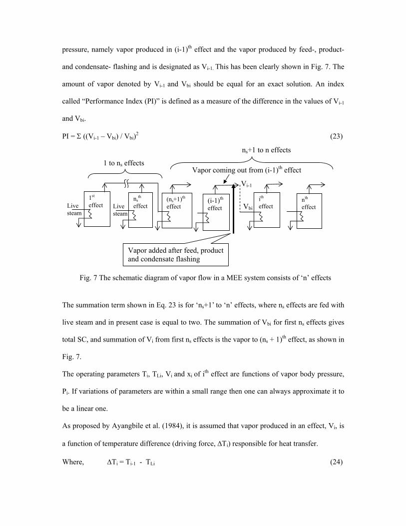
pressure, namely vapor produced in (i-1)th effect and the vapor produced by feed-, product-

and condensate- flashing and is designated as Vi-1. This has been clearly shown in Fig. 7. The

amount of vapor denoted by Vi-1 and Vbi should be equal for an exact solution. An index

called “Performance Index (PI)” is defined as a measure of the difference in the values of Vi-1

and Vbi.

PI = Σ ((Vi-1 – Vbi) / Vbi)2 (23)

The summation term shown in Eq. 23 is for ‘ns+1’ to ‘n’ effects, where ns effects are fed with

live steam and in present case is equal to two. The summation of Vbi for first ns effects gives

total SC, and summation of Vi from first ns effects is the vapor to (ns + 1)th effect, as shown in

Fig. 7.

The operating parameters Ti, TLi, Vi and xi of ith effect are functions of vapor body pressure,

Pi. If variations of parameters are within a small range then one can always approximate it to

be a linear one.

As proposed by Ayangbile et al. (1984), it is assumed that vapor produced in an effect, Vi, is

a function of temperature difference (driving force, ΔΤi) responsible for heat transfer.

Where, ΔTi = Ti-1 - TLi (24)

1st effect

nsth

effect (ns+1)th effect

(i-1)th effect

ith effect

nth effect Live

steam Live steam

1 to ns effects

ns+1 to n effects

Fig. 7 The schematic diagram of vapor flow in a MEE system consists of ‘n’ effects

Vapor added after feed, product and condensate flashing

Vapor coming out from (i-1)th effect

Vi-1

Vbi

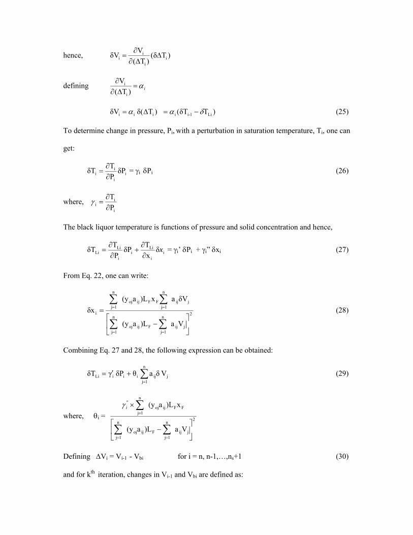
hence, )Tδ()T(

VδV ii

ii Δ

Δ∂∂

=

defining iα=Δ∂

∂)T(

V

i

i

)Tδ( δV iii Δ= α )TδT( Li1-ii δα −= (25)

To determine change in pressure, Pi, with a perturbation in saturation temperature, Ti, one can

get:

ii

ii δP

PTδT

∂∂

= = γi δPi (26)

where, i

ii P

T∂∂

=γ

The black liquor temperature is functions of pressure and solid concentration and hence,

ii

Lii

i

LiLi δ

xTδP

PTδT x

∂∂

+∂∂

= = γi’ δPi + γi” δxi (27)

From Eq. 22, one can write:

2

jij

n

1jFijoj

n

1j

jij

n

1jFFijoj

n

1ji

Va)La(y

δVax)La(yδx

⎥⎦

⎤⎢⎣

⎡−

=

∑∑

∑∑

==

== (28)

Combining Eq. 27 and 28, the following expression can be obtained:

∑=

+′=n

1jjijiiiLi V δa θδP γδT (29)

where, θi = 2

jij

n

1jFijoj

n

1j

FFijoj

n

1j

''

Va)La(y

x)La(y

⎥⎦

⎤⎢⎣

⎡−

×

∑∑

∑

==

=iγ

Defining ΔVi = Vi-1 - Vbi for i = n, n-1,…,ns+1 (30)

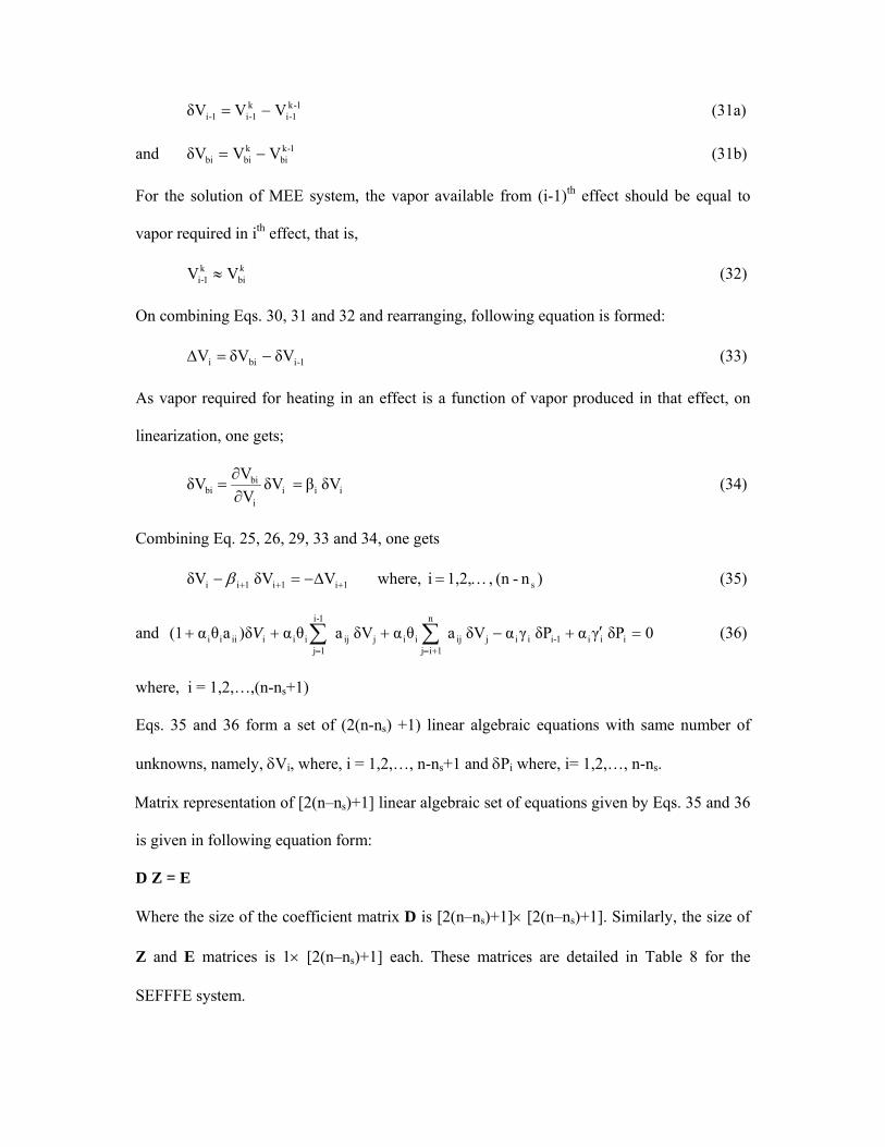
and for kth iteration, changes in Vi-1 and Vbi are defined as:

1-k1-i

k1-i1-i VVδV −= (31a)

and 1-kbi

kbibi VVδV −= (31b)

For the solution of MEE system, the vapor available from (i-1)th effect should be equal to

vapor required in ith effect, that is,

kbi

k1-i VV ≈ (32)

On combining Eqs. 30, 31 and 32 and rearranging, following equation is formed:

1-ibii δVδVV −=Δ (33)

As vapor required for heating in an effect is a function of vapor produced in that effect, on

linearization, one gets;

ii

bibi δV

VVδV

∂∂

= ii δV β= (34)

Combining Eq. 25, 26, 29, 33 and 34, one gets

)n-(n ,1,2, i re, wheVδV δV s1i1i1ii …=Δ−=− +++β (35)

and 0δP γαδP γαδV aθαδV aθα)δaθα(1 iii1-iiijij

n

1ijiijij

1-i

1jiiiiiii =′+−+++ ∑∑

+==

V (36)

where, i = 1,2,…,(n-ns+1)

Eqs. 35 and 36 form a set of (2(n-ns) +1) linear algebraic equations with same number of

unknowns, namely, δVi, where, i = 1,2,…, n-ns+1 and δPi where, i= 1,2,…, n-ns.

Matrix representation of [2(n–ns)+1] linear algebraic set of equations given by Eqs. 35 and 36

is given in following equation form:

D Z = E

Where the size of the coefficient matrix D is [2(n–ns)+1]× [2(n–ns)+1]. Similarly, the size of

Z and E matrices is 1× [2(n–ns)+1] each. These matrices are detailed in Table 8 for the

SEFFFE system.

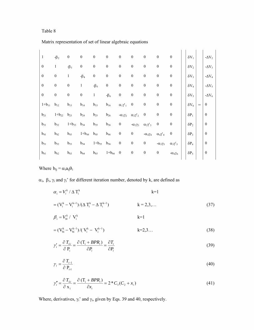
Table 8 Matrix representation of set of linear algebraic equations

1 -β2 0 0 0 0 0 0 0 0 0 δV1 -ΔV2

0 1 -β3 0 0 0 0 0 0 0 0 δV2 -ΔV3

0 0 1 -β4 0 0 0 0 0 0 0 δV3 -ΔV4

0 0 0 1 -β5 0 0 0 0 0 0 δV4 -ΔV5

0 0 0 0 1 -β6 0 0 0 0 0 δV5 -ΔV6

1+b11 b12 b13 b14 b15 b16 α1γ′1 0 0 0 0 δV6 = 0

b21 1+b22 b23 b24 b25 b26 -α2γ2 α2γ′2 0 0 0 δP1 0

b31 b32 1+b33 b34 b35 b36 0 -α3γ3 α3γ′3 0 0 δP2 0

b41 b42 b43 1+b44 b45 b46 0 0 -α4γ4 α4γ′4 0 δP3 0

b51 b52 b53 b54 1+b55 b56 0 0 0 -α5γ5 α5γ′5 δP4 0

b61 b62 b63 b64 b65 1+b66 0 0 0 0 -α6γ6 δP5 0

Where bij = αiaijθi

αi, βi, γi and γi’ for different iteration number, denoted by k, are defined as

kii T / Δ= k

iVα k=1

)T T /()VV( 1ki

ki

1ki

ki

−− Δ−Δ−= k = 2,3,… (37)

kii V /k

biV=β k=1

)V V /()VV( 1ki

ki

1kbi

kbi

−− −−= k=2,3… (38)

i

i

i

iLii P

TPBPRT

∂∂

=∂+∂

=∂∂

=′ )(T P i

i

γ (39)

1-i

1

P

∂∂

= −ii

Tγ (40)

)(*2)(T

x

23i

ii

i

iLii xCC

xBPRT

+=∂+∂

=∂∂

=′′γ (41)

Where, derivatives, γi’ and γi, given by Eqs. 39 and 40, respectively.

By solving Eqs. 35 and 36, one can obtain the values of δPi, where, i = 1,2,…,(n-ns). The

values of δPi, so obtained, are used to modify the pressure of all the effects except last effect-

the pressure of which is kept at a fixed value.

This process is to be repeated iteratively till desired precision (5*10-6) in the value of PI is

obtained.

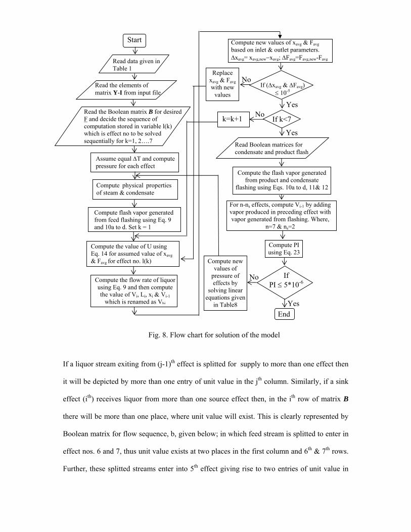
4. Solution of the model For the solution of the model, developed in the present investigation, a computer program is

developed in FORTRAN 90 and run on Pentium IV machine, using Microsoft FORTRAN

Power Station 4.0 compiler. The flow chart of the algorithm is shown in Fig. 8.

For the generalized cascade algorithm the equation developed for an effect is solved

repeatedly for different effects depending upon the sequence of computation determined by

the selected F which in turn is decided by the Boolean matrix B.

For the SEFFFE system, order of the matrix is 8×8, where the first column denotes the feed

stream and subsequent columns are source effects 1 to 7 and first 7 rows are sink effects and

last row is product stream. A unit value of element bij indicates that liquor exiting from ( j-1)th

effect enters ith effect. The backward F is represented by the Boolean matrix, given below, in

which element b13 = 1 shows that liquor exits from 2nd effect and enters first effect.

(Feed) F 1 2 3 4 5 6 7

B =

⎥⎥⎥⎥⎥⎥⎥⎥⎥⎥⎥

⎦

⎤

⎢⎢⎢⎢⎢⎢⎢⎢⎢⎢⎢

⎣

⎡

0000000010000100

0010000100000000

0010000100000000

0000000010000100

P7654321

Source effect Sink effect

(Product)

If a liquor stream exiting from (j-1)th effect is splitted for supply to more than one effect then

it will be depicted by more than one entry of unit value in the jth column. Similarly, if a sink

effect (ith) receives liquor from more than one source effect then, in the ith row of matrix B

there will be more than one place, where unit value will exist. This is clearly represented by

Boolean matrix for flow sequence, b, given below; in which feed stream is splitted to enter in

effect nos. 6 and 7, thus unit value exists at two places in the first column and 6th & 7th rows.

Further, these splitted streams enter into 5th effect giving rise to two entries of unit value in

Start

Read data given in Table 1

Read the elements of matrix Y-I from input file

Read the Boolean matrix B for desired F and decide the sequence of computation stored in variable l(k) which is effect no to be solved sequentially for k=1, 2….7

Compute the value of U using Eq. 14 for assumed value of xavg & Favg for effect no. l(k)

Compute the flow rate of liquor using Eq. 9 and then compute the value of Vi, Li, xi & Vi-1

which is renamed as Vbi

If (Δxavg & ΔFavg) ≤ 10-5

Read Boolean matrices for condensate and product flash

Compute the flash vapor generated from product and condensate

flashing using Eqs. 10a to d, 11& 12

For n-ns effects, compute Vi-1 by adding vapor produced in preceding effect with vapor generated from flashing. Where,

n=7 & ns=2

Compute PI using Eq. 23

If PI ≤ 5*10-6

End

No

Yes

Yes

Compute new values of

pressure of effects by

solving linear equations given

in Table8

No

Fig. 8. Flow chart for solution of the model

Assume equal ΔT and compute pressure for each effect

Compute flash vapor generated from feed flashing using Eq. 9 and 10a to d. Set k = 1

Replace xavg & Favg with new

values

If k<7 k=k+1

Compute physical properties of steam & condensate

Compute new values of xavg & Favg based on inlet & outlet parameters. Δxavg= xavg,new−xavg; ΔFavg=Favg,new-Favg

No

Yes

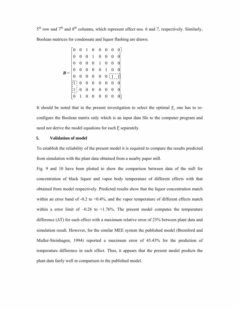
5th row and 7th and 8th columns, which represent effect nos. 6 and 7, respectively. Similarly,

Boolean matrices for condensate and liquor flashing are drawn.

B =

⎥⎥⎥⎥⎥⎥⎥⎥⎥⎥⎥

⎦

⎤

⎢⎢⎢⎢⎢⎢⎢⎢⎢⎢⎢

⎣

⎡

0000000000001100

0010000100010000

0010000100000000

0000000010000100

It should be noted that in the present investigation to select the optimal F, one has to re-

configure the Boolean matrix only which is an input data file to the computer program and

need not derive the model equations for each F separately.

5. Validation of model

To establish the reliability of the present model it is required to compare the results predicted

from simulation with the plant data obtained from a nearby paper mill.

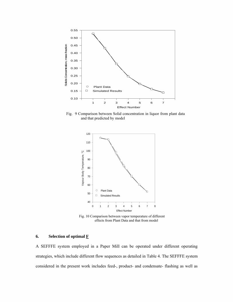
Fig. 9 and 10 have been plotted to show the comparison between data of the mill for

concentration of black liquor and vapor body temperature of different effects with that

obtained from model respectively. Predicted results show that the liquor concentration match

within an error band of -0.2 to +0.4%, and the vapor temperature of different effects match

within a error limit of –0.26 to +1.76%. The present model computes the temperature

difference (ΔT) for each effect with a maximum relative error of 23% between plant data and

simulation result. However, for the similar MEE system the published model (Bremford and

Muller-Steinhagen, 1994) reported a maximum error of 43.43% for the prediction of

temperature difference in each effect. Thus, it appears that the present model predicts the

plant data fairly well in comparison to the published model.

6. Selection of optimal F

A SEFFFE system employed in a Paper Mill can be operated under different operating

strategies, which include different flow sequences as detailed in Table 4. The SEFFFE system

considered in the present work includes feed-, product- and condensate- flashing as well as

Fig 5.3

Effect Number

0 1 2 3 4 5 6 7 8

Sol

ids

Con

cent

ratio

n, m

ass

fract

ion

0.10

0.15

0.20

0.25

0.30

0.35

0.40

0.45

0.50

0.55

Plant DataSimulated Results

Fig. 9 Comparison between Solid concentration in liquor from plant data and that predicted by model

Fig 5.4

Effect Number

0 1 2 3 4 5 6 7 8

Vapo

ur B

ody

Tem

pera

ture

, o C

40

50

60

70

80

90

100

110

120

Plant Data

Simulated Results

Fig. 10 Comparison between vapor temperature of different effects from Plant Data and that from model

feed and steam splitting. Out of the above referred operating strategies, selection of proper F,

which will provide maximum SE, is the aim of the present study. In fact, in real situation, the

best F is not only decided by SE but also based on other parameters such as foaming of feed,

scaling of tubes, etc. Nevertheless, grading of F based on SE has always been an important

step towards finalization of best flow sequence which depends on SE data and operating

convenience.

To screen the optimal F amongst the feasible F, it is necessary to study the effect of variation

of input parameters T0 and F on output parameter, SC and SE. It will help to select an optimal

F, which will remain as optimal for complete range of operating parameters given in Table 2.

It is well known fact that a change in input parameters triggers a complex chain reaction

affecting almost all output parameters, including, vapor body and liquor temperatures from

first to sixth effect, almost all flash vapor fractions, heat transfer coefficients, rate of

evaporation in each effect, Qloss from each effect and amount of heat rejected to atmosphere

with condensate. It appears that SE is the single most prominent parameter to evaluate the

efficiency of the system as it varies with variation in operating parameters and geometrical

parameters as well. SE also directly affects the economy of the operation. Nevertheless, the

study of variables towards the variation of SC with input parameter offers better

understanding.

6.1. Effect of variations of T0 and F on SC and SE for all F

An investigation based on the present model has been undertaken to study the effect of steam

temperature, T0, and feed flow rate, F, on SC and SE, which is carried out for different flow

sequences a, b, c, d, e and f as defined in Table 4.

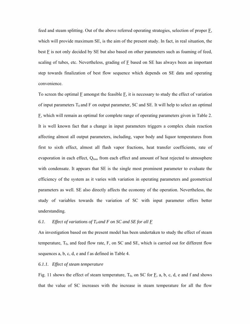
6.1.1. Effect of steam temperature

Fig. 11 shows the effect of steam temperature, T0, on SC for F, a, b, c, d, e and f and shows

that the value of SC increases with the increase in steam temperature for all the flow

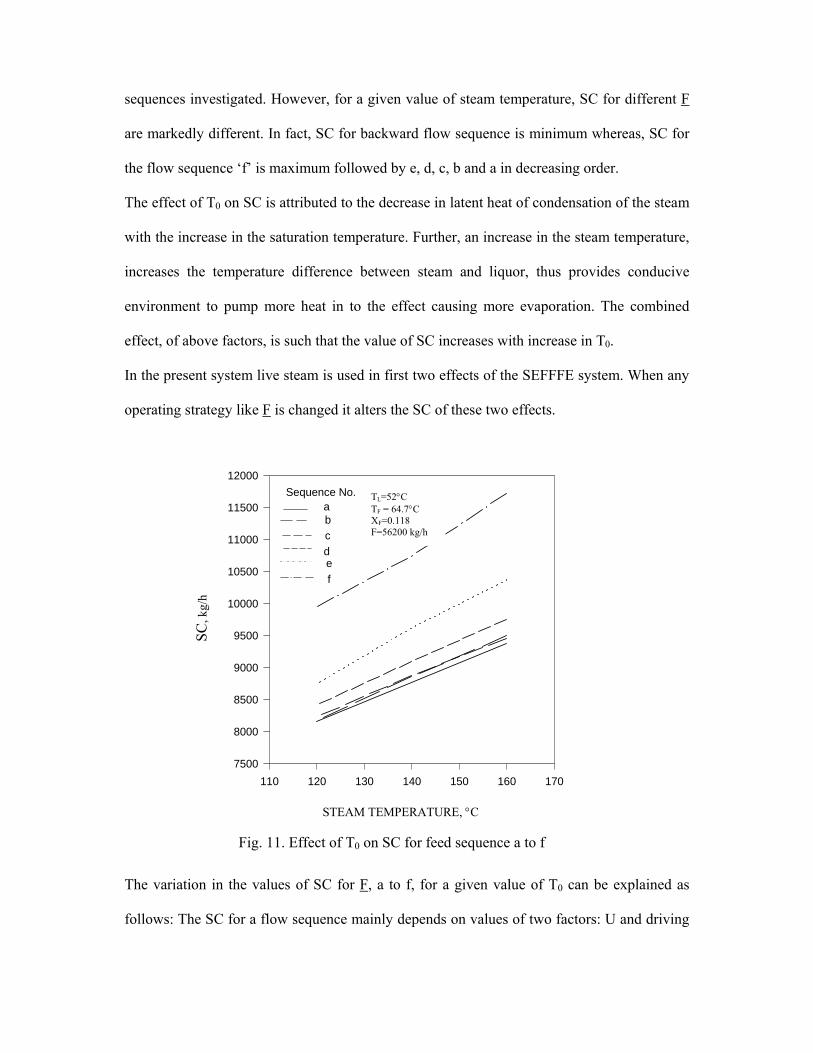
sequences investigated. However, for a given value of steam temperature, SC for different F

are markedly different. In fact, SC for backward flow sequence is minimum whereas, SC for

the flow sequence ‘f’ is maximum followed by e, d, c, b and a in decreasing order.

The effect of T0 on SC is attributed to the decrease in latent heat of condensation of the steam

with the increase in the saturation temperature. Further, an increase in the steam temperature,

increases the temperature difference between steam and liquor, thus provides conducive

environment to pump more heat in to the effect causing more evaporation. The combined

effect, of above factors, is such that the value of SC increases with increase in T0.

In the present system live steam is used in first two effects of the SEFFFE system. When any

operating strategy like F is changed it alters the SC of these two effects.

The variation in the values of SC for F, a to f, for a given value of T0 can be explained as

follows: The SC for a flow sequence mainly depends on values of two factors: U and driving

Fig. Effect of TS on SC for feed sequences a to fSTEAM TEMPERATURE, oC

110 120 130 140 150 160 170

SC, k

g/ h

7500

8000

8500

9000

9500

10000

10500

11000

11500

12000Sequence No.

abcdef

STEAM TEMPERATURE, °C

Fig. 11. Effect of T0 on SC for feed sequence a to f

SC, k

g/h

TL=52°C TF = 64.7°C XF=0.118 F=56200 kg/h

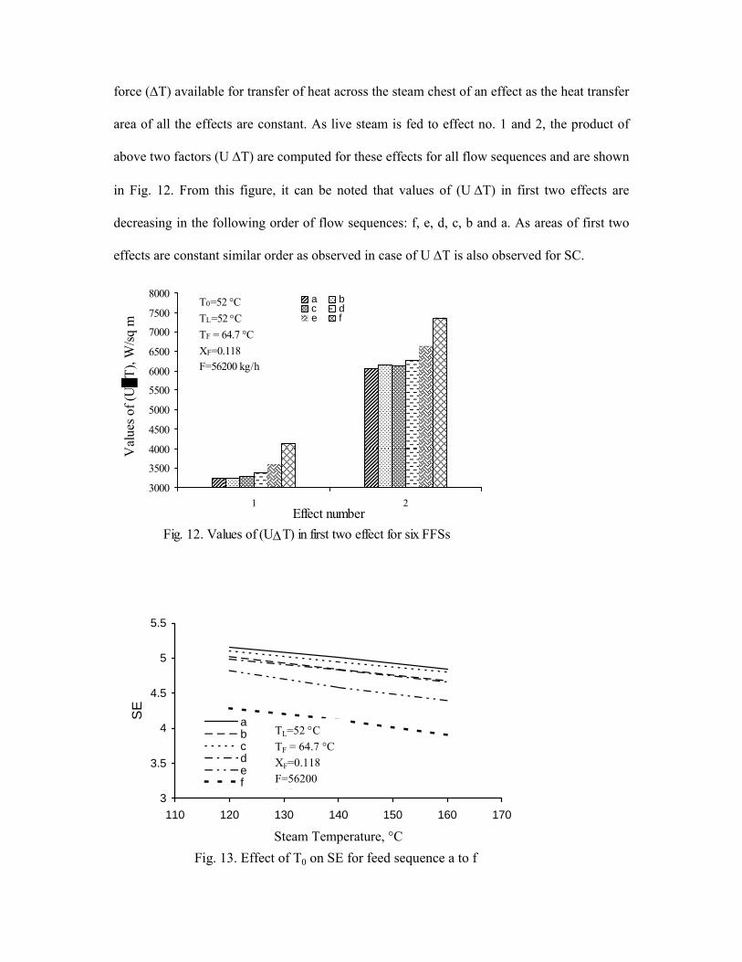
force (ΔT) available for transfer of heat across the steam chest of an effect as the heat transfer

area of all the effects are constant. As live steam is fed to effect no. 1 and 2, the product of

above two factors (U ΔT) are computed for these effects for all flow sequences and are shown

in Fig. 12. From this figure, it can be noted that values of (U ΔT) in first two effects are

decreasing in the following order of flow sequences: f, e, d, c, b and a. As areas of first two

effects are constant similar order as observed in case of U ΔT is also observed for SC.

Fig. 12. Values of (UΔT) in first two effect for six FFSs

3000

3500

4000

4500

5000

5500

6000

6500

7000

7500

8000

1 2Effect number

Val

ues o

f (U

T),

W/sq

m

a bc de f

T0=52 °CTL=52 °C TF = 64.7 °CXF=0.118F=56200 kg/h

Fig. 13. Effect of T0 on SE for feed sequence a to f

3

3.5

4

4.5

5

5.5

110 120 130 140 150 160 170

Steam Temperature, °C

SE

abcdef

TL=52 °C TF = 64.7 °CXF=0.118F=56200 k /h

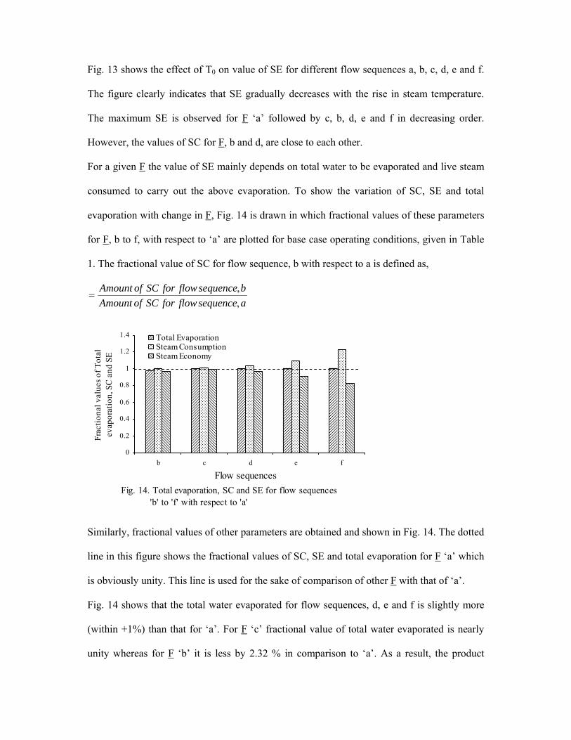
Fig. 13 shows the effect of T0 on value of SE for different flow sequences a, b, c, d, e and f.

The figure clearly indicates that SE gradually decreases with the rise in steam temperature.

The maximum SE is observed for F ‘a’ followed by c, b, d, e and f in decreasing order.

However, the values of SC for F, b and d, are close to each other.

For a given F the value of SE mainly depends on total water to be evaporated and live steam

consumed to carry out the above evaporation. To show the variation of SC, SE and total

evaporation with change in F, Fig. 14 is drawn in which fractional values of these parameters

for F, b to f, with respect to ‘a’ are plotted for base case operating conditions, given in Table

1. The fractional value of SC for flow sequence, b with respect to a is defined as,

asequenceflowforSCofAmountbsequenceflowforSCofAmount

,,

=

Fig. 14. Total evaporation, SC and SE for flow sequences 'b' to 'f' with respect to 'a'

0

0.2

0.4

0.6

0.8

1

1.2

1.4

b c d e f

Flow sequences

Frac

tiona

l val

ues o

f Tot

alev

apor

atio

n, S

C a

nd S

E

Total EvaporationSteam ConsumptionSteam Economy

Similarly, fractional values of other parameters are obtained and shown in Fig. 14. The dotted

line in this figure shows the fractional values of SC, SE and total evaporation for F ‘a’ which

is obviously unity. This line is used for the sake of comparison of other F with that of ‘a’.

Fig. 14 shows that the total water evaporated for flow sequences, d, e and f is slightly more

(within +1%) than that for ‘a’. For F ‘c’ fractional value of total water evaporated is nearly

unity whereas for F ‘b’ it is less by 2.32 % in comparison to ‘a’. As a result, the product

concentration, xP, is different for different F. However, the fractional values of SC for F, ‘b’

to ‘f’ are greater than unity and continuously increase from F, ‘b’ to ‘f’. It is clear from Fig.

14 that the increase in the value of SC is much more than increase in total evaporation for F,

d, e and f in comparison to ‘a’. Hence, the values of SE for these F are considerably less. It is

also noted from Fig. 14, that total evaporation for flow sequence, ‘c’ is equal to that of ‘a’,

whereas, SC for ‘c’ is greater by 1.2% in comparison to ‘a’. The cumulative effects of these

factors lower the value of SE for flow sequence ‘c’. It is further observed from Fig. 14, that

for F ‘b’ total evaporation is less and SC is slightly more than that for ‘a’. As a result of it the

value of SE is lowest for F ‘b’.

6.1.2. Effect of feed flow rate

Table 9 shows the effect of variation of feed flow rate on UΔT, total evaporation, SC and SE

for different flow sequences a, b, c, d, e and f.

Table 9 shows that the value of SC increases with the increase in black liquor feed rate. For

lowest value of feed flow rate, the SC is highest for F, f followed by e, d, c, b and a in

decreasing order. However, at highest flow rate the F f, e, d, c, a and b are in order of

decreasing value of SC.

Further, Table 9 indicates that for a flow sequence the value of SE decreases with increase in

feed flow rate and the maximum SE is observed for the F ‘a’ followed by c, b, d, e and f.

When feed flow rate is increased the U of different effects increase. This in turn increases

heat flow to each effect and causes the temperature of each effect to increase due to formation

of higher amount of vapor in each effect, which subsequently pressurizes the vapor body to

some extent. This rise in temperature will have a reverse effect on heat transfer rate as it

decreases the driving force ΔT. However, the overall effect will be governed by the product

UΔT. As the behaviors of first two effects affect the SC most, UΔT values of only these

effects are reported in Table 9. From the simulated results, shown in Table 9, it is evident that

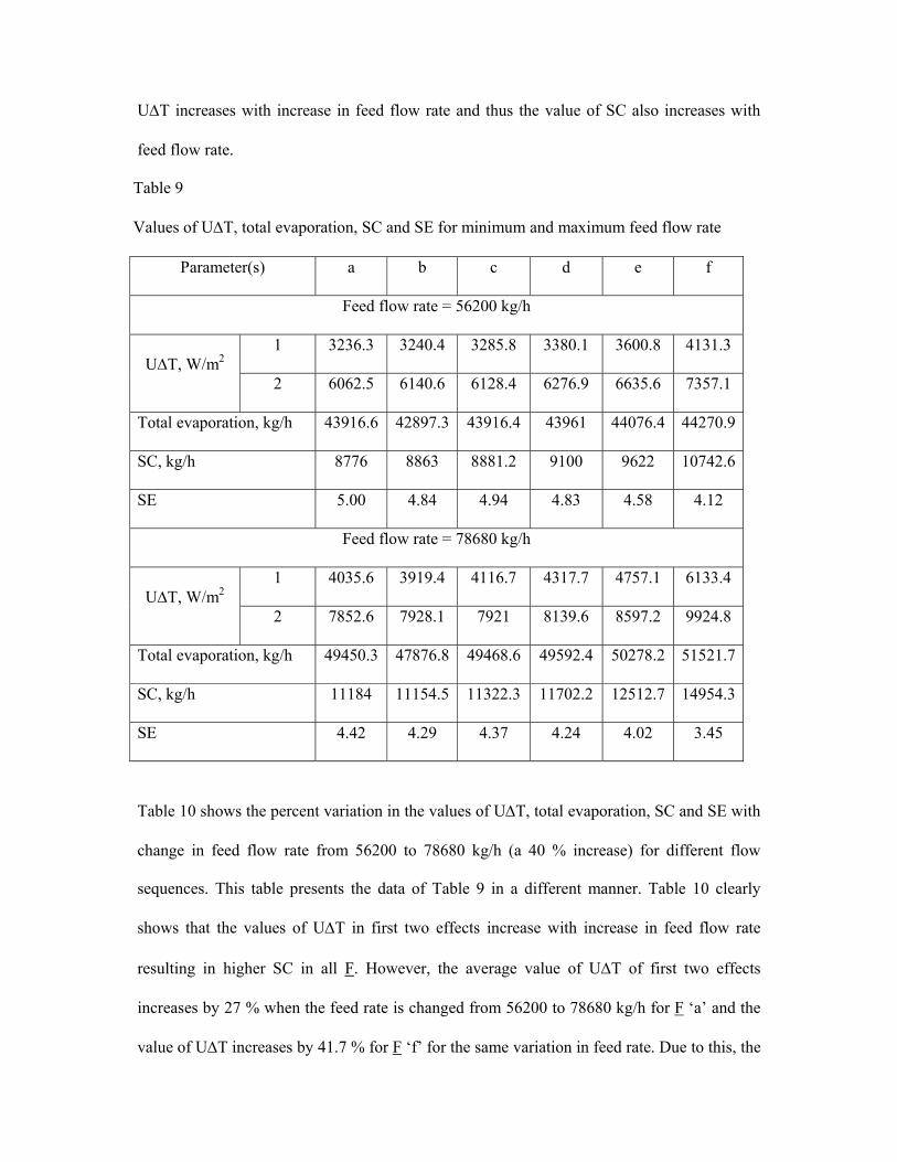
UΔT increases with increase in feed flow rate and thus the value of SC also increases with

feed flow rate.

Table 9

Values of UΔT, total evaporation, SC and SE for minimum and maximum feed flow rate

Parameter(s) a b c d e f

Feed flow rate = 56200 kg/h

UΔT, W/m2 1 3236.3 3240.4 3285.8 3380.1 3600.8 4131.3

2 6062.5 6140.6 6128.4 6276.9 6635.6 7357.1

Total evaporation, kg/h 43916.6 42897.3 43916.4 43961 44076.4 44270.9

SC, kg/h 8776 8863 8881.2 9100 9622 10742.6

SE 5.00 4.84 4.94 4.83 4.58 4.12

Feed flow rate = 78680 kg/h

UΔT, W/m2 1 4035.6 3919.4 4116.7 4317.7 4757.1 6133.4

2 7852.6 7928.1 7921 8139.6 8597.2 9924.8

Total evaporation, kg/h 49450.3 47876.8 49468.6 49592.4 50278.2 51521.7

SC, kg/h 11184 11154.5 11322.3 11702.2 12512.7 14954.3

SE 4.42 4.29 4.37 4.24 4.02 3.45

Table 10 shows the percent variation in the values of UΔT, total evaporation, SC and SE with

change in feed flow rate from 56200 to 78680 kg/h (a 40 % increase) for different flow

sequences. This table presents the data of Table 9 in a different manner. Table 10 clearly

shows that the values of UΔT in first two effects increase with increase in feed flow rate

resulting in higher SC in all F. However, the average value of UΔT of first two effects

increases by 27 % when the feed rate is changed from 56200 to 78680 kg/h for F ‘a’ and the

value of UΔT increases by 41.7 % for F ‘f’ for the same variation in feed rate. Due to this, the

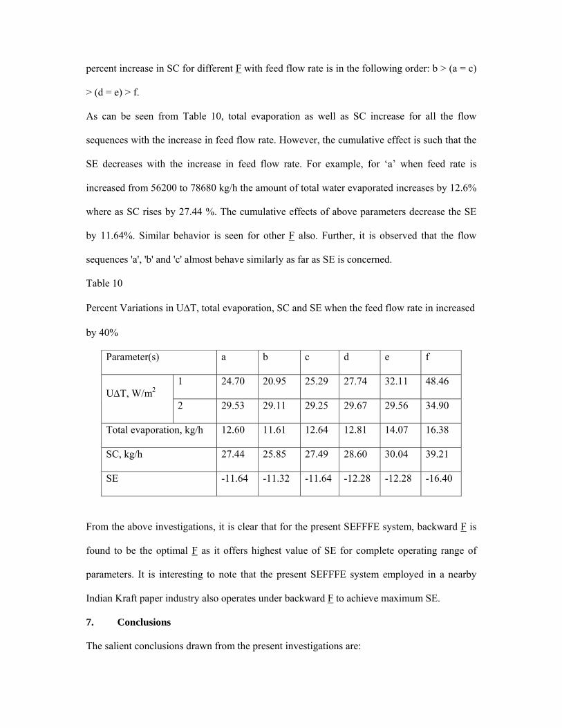
percent increase in SC for different F with feed flow rate is in the following order: b > (a = c)

> (d = e) > f.

As can be seen from Table 10, total evaporation as well as SC increase for all the flow

sequences with the increase in feed flow rate. However, the cumulative effect is such that the

SE decreases with the increase in feed flow rate. For example, for ‘a’ when feed rate is

increased from 56200 to 78680 kg/h the amount of total water evaporated increases by 12.6%

where as SC rises by 27.44 %. The cumulative effects of above parameters decrease the SE

by 11.64%. Similar behavior is seen for other F also. Further, it is observed that the flow

sequences 'a', 'b' and 'c' almost behave similarly as far as SE is concerned.

Table 10

Percent Variations in UΔT, total evaporation, SC and SE when the feed flow rate in increased

by 40%

Parameter(s) a b c d e f

UΔT, W/m2 1 24.70 20.95 25.29 27.74 32.11 48.46

2 29.53 29.11 29.25 29.67 29.56 34.90

Total evaporation, kg/h 12.60 11.61 12.64 12.81 14.07 16.38

SC, kg/h 27.44 25.85 27.49 28.60 30.04 39.21

SE -11.64 -11.32 -11.64 -12.28 -12.28 -16.40

From the above investigations, it is clear that for the present SEFFFE system, backward F is

found to be the optimal F as it offers highest value of SE for complete operating range of

parameters. It is interesting to note that the present SEFFFE system employed in a nearby

Indian Kraft paper industry also operates under backward F to achieve maximum SE.

7. Conclusions

The salient conclusions drawn from the present investigations are:

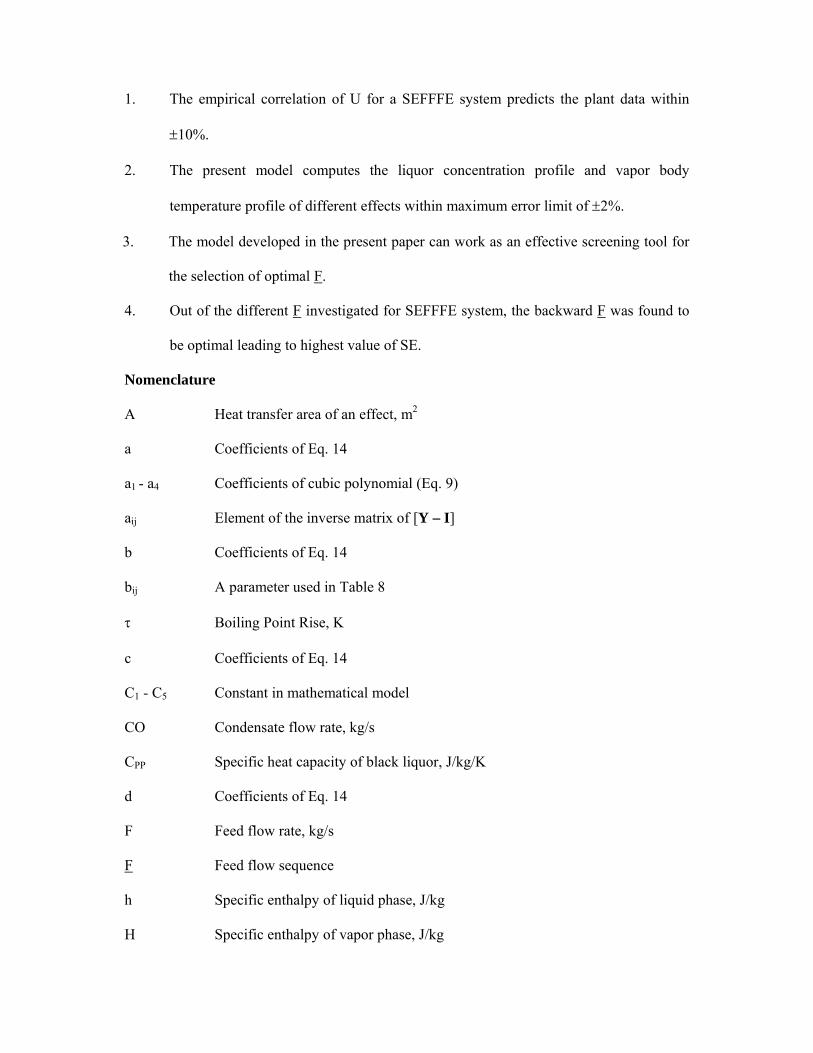
1. The empirical correlation of U for a SEFFFE system predicts the plant data within

±10%.

2. The present model computes the liquor concentration profile and vapor body

temperature profile of different effects within maximum error limit of ±2%.

3. The model developed in the present paper can work as an effective screening tool for

the selection of optimal F.

4. Out of the different F investigated for SEFFFE system, the backward F was found to

be optimal leading to highest value of SE.

Nomenclature

A Heat transfer area of an effect, m2

a Coefficients of Eq. 14

a1 - a4 Coefficients of cubic polynomial (Eq. 9)

aij Element of the inverse matrix of [Y – I]

b Coefficients of Eq. 14

bij A parameter used in Table 8

τ Boiling Point Rise, K

c Coefficients of Eq. 14

C1 - C5 Constant in mathematical model

CO Condensate flow rate, kg/s

CPP Specific heat capacity of black liquor, J/kg/K

d Coefficients of Eq. 14

F Feed flow rate, kg/s

F Feed flow sequence

h Specific enthalpy of liquid phase, J/kg

H Specific enthalpy of vapor phase, J/kg

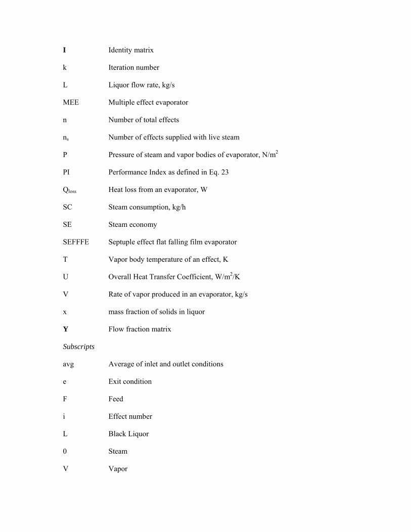
I Identity matrix

k Iteration number

L Liquor flow rate, kg/s

MEE Multiple effect evaporator

n Number of total effects

ns Number of effects supplied with live steam

P Pressure of steam and vapor bodies of evaporator, N/m2

PI Performance Index as defined in Eq. 23

Qloss Heat loss from an evaporator, W

SC Steam consumption, kg/h

SE Steam economy

SEFFFE Septuple effect flat falling film evaporator

T Vapor body temperature of an effect, K

U Overall Heat Transfer Coefficient, W/m2/K

V Rate of vapor produced in an evaporator, kg/s

x mass fraction of solids in liquor

Y Flow fraction matrix

Subscripts

avg Average of inlet and outlet conditions

e Exit condition

F Feed

i Effect number

L Black Liquor

0 Steam

V Vapor

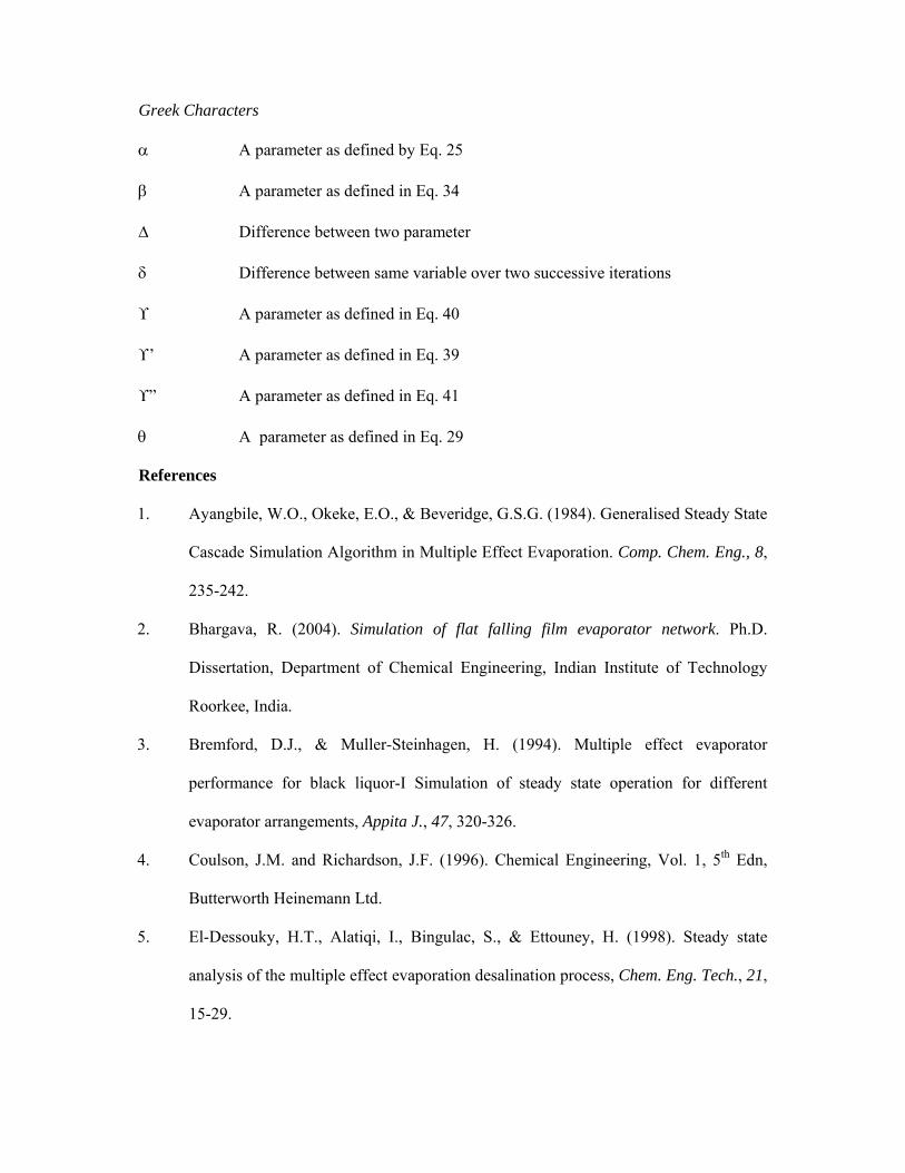
Greek Characters

α A parameter as defined by Eq. 25

β A parameter as defined in Eq. 34

Δ Difference between two parameter

δ Difference between same variable over two successive iterations

ϒ A parameter as defined in Eq. 40

ϒ’ A parameter as defined in Eq. 39

ϒ” A parameter as defined in Eq. 41

θ A parameter as defined in Eq. 29

References

1. Ayangbile, W.O., Okeke, E.O., & Beveridge, G.S.G. (1984). Generalised Steady State

Cascade Simulation Algorithm in Multiple Effect Evaporation. Comp. Chem. Eng., 8,

235-242.

2. Bhargava, R. (2004). Simulation of flat falling film evaporator network. Ph.D.

Dissertation, Department of Chemical Engineering, Indian Institute of Technology

Roorkee, India.

3. Bremford, D.J., & Muller-Steinhagen, H. (1994). Multiple effect evaporator

performance for black liquor-I Simulation of steady state operation for different

evaporator arrangements, Appita J., 47, 320-326.

4. Coulson, J.M. and Richardson, J.F. (1996). Chemical Engineering, Vol. 1, 5th Edn,

Butterworth Heinemann Ltd.

5. El-Dessouky, H.T., Alatiqi, I., Bingulac, S., & Ettouney, H. (1998). Steady state

analysis of the multiple effect evaporation desalination process, Chem. Eng. Tech., 21,

15-29.

6. El-Dessouky, H.T., Ettouney, H.M., & Al-Juwayhel, F. (2000). Multiple effect

evaporation-vapor compression desalination processes, Trans IChemE, 78, Part A,

662-676.

7. Harper, J.M., & Tsao, T.F. (1972). Evaporator strategy and optimization. In Computer

Programs for Chemical Engineering Education, VI Design, Ed. R. Jelinek, Aztec

Publishing, Austin, Texas.

8. Holland, C.D. (1975). Fundamentals and Modelling of Separation Processes. Prentice

Hall Inc., Englewood cliffs, New Jersey.

9. Itahara, S., & Stiel, L.I. (1966). Optimal Design of Multiple Effect Evaporators by

Dynamic Programming, Ind. Eng. Chem. Proc. Des. Dev., 5, 309.

10. Kern, D.Q. (1950). Process Heat Transfer, McGraw Hill.

11. Lambert, R.N., Joye, D.D., & Koko, F.W. (1987). Design calculations for multiple

effect evaporators-I linear methods, Ind. Eng. Chem. Res., 26, 100-104.

12. Mathur, T.N.S. (1992). Energy Conservation Studies for the Multiple Effect

Evaporator House of Pulp and Paper Mills. Ph.D. Dissertation, Department of

Chemical Engineering, University of Roorkee, India.

13. Nishitani, H., & Kunugita, E. (1979). The optimal flow pattern of multiple effect

evaporator systems. Comp. Chem. Eng., 3, 261-268.

14. Radovic, L.R., Tasic, A.Z., Grozanic, D.K., Djordjevic, B.D., & Valent, V.J. (1979).

Computer design and analysis of operation of a multiple effect evaporator system in

the sugar industry, Ind. Eng. Chem. Proc. Des. Dev, 18, 318-323.

15. Rao, N. J., & Kumar, R. (1985). Energy Conservation Approaches in a Paper Mill

with Special Reference to the Evaporator Plant. Proc. IPPTA Int. Seminar on Energy

Conservation in Pulp and Paper Industry, New Delhi, India, 58-70.

16. Ray, A.K., Rao, N.J., Bansal, M.C., & Mohanty, B. (1992). Design Data and

Correlations of Waste Liquor/Black Liquor from Pulp Mills”, IPPTA J., 4, 1-21.

17. Ray, A.K., & Singh, P. (2000). Simulation of Multiple Effect Evaporator for Black

Liquor Concentration, IPPTA J., 12, 53-63.

18. Stewart, G., & Beveridge, G. S. G. (1977). Steady State Cascade Simulation in

Multiple Effect Evaporation. Comp. Chem. Eng., 1, 3-9.

19. Süren, A. (1995). Scaling of black liquor in a falling film evaporator, Master Thesis,

Georgia Institute of Technology, Atlanta, GA.