Embed Size (px)
Citation preview
arX
iv:0
707.
0530
v3 [
gr-q
c] 2
Jan
200
8
Self-similar cosmological solutions with dark energy. II:
black holes, naked singularities and wormholes
1,2,3,4Hideki Maeda∗, 4Tomohiro Harada†, and 5,6B. J. Carr‡1Centro de Estudios Cientıficos (CECS), Arturo Prat 514, Valdivia, Chile
2Department of Physics, International Christian University,3-10-2 Osawa, Mitaka-shi, Tokyo 181-8585, Japan
3Graduate School of Science and Engineering, Waseda University, Tokyo 169-8555, Japan4Department of Physics, Rikkyo University, Tokyo 171-8501, Japan
5Astronomy Unit, Queen Mary, University of London, Mile End Road, London E1 4NS, UK6Research Center for the Early Universe, Graduate School of Science, University of Tokyo, Tokyo 113-0033, Japan
(Dated: February 16, 2013)
We use a combination of numerical and analytical methods, exploiting the equations derived in apreceding paper, to classify all spherically symmetric self-similar solutions which are asymptoticallyFriedmann at large distances and contain a perfect fluid with equation of state p = (γ − 1)µ with0 < γ < 2/3. The expansion of the Friedmann universe is accelerated in this case. We find aone-parameter family of self-similar solutions representing a black hole embedded in a Friedmannbackground. This suggests that, in contrast to the positive pressure case, black holes in a universewith dark energy can grow as fast as the Hubble horizon if they are not too large. There are alsoself-similar solutions which contain a central naked singularity with negative mass and solutionswhich represent a Friedmann universe connected to either another Friedmann universe or someother cosmological model. The latter are interpreted as self-similar cosmological white hole orwormhole solutions. The throats of these wormholes are defined as two-dimensional spheres withminimal area on a spacelike hypersurface and they are all non-traversable because of the absence ofa past null infinity.
PACS numbers: 04.70.Bw, 95.36.+x, 97.60.Lf, 04.40.Nr, 04.25.Dm
I. INTRODUCTION
The study of black holes in stationary and asymptoti-cally flat spacetimes has led to many remarkable insights,such as the “no hair” theorem and the discovery of thethermodynamic properties of black holes. In contrast,black holes in a Friedmann background have not beenfully investigated and many important open questionsremain. When the size of the black hole is much smallerthan the cosmological horizon, asymptotically flat blackhole solutions will presumably provide a good approxima-tion. However, for black holes comparable to the horizonsize – such as primordial black holes (PBHs) formed inthe early universe [1] – one would need to take into ac-count the effects of the cosmological expansion.
The main issue addressed in this paper is the growthof such “cosmological” black holes. Zel’dovich andNovikov [2] first discussed the possibility of self-similargrowth for a black hole in a Friedmann universe in 1967.This suggested that the size of a PBH might always bethe same fraction of the size of the particle horizon untilthe end of the radiation-dominated era, when they wouldhave a mass of order 1015M⊙. Since there is no evidencethat such huge black holes exist, this seemed to implythat PBHs never formed at all. More recently, the possi-
∗Electronic address:[email protected]†Electronic address:[email protected]‡Electronic address:[email protected]
bility of self-similar PBH growth in the quintessence sce-nario has led to the suggestion that PBHs could provideseeds for the supermassive black holes thought to residein galactic nuclei [3]. However, both these arguments arebased on a simple Newtonian analysis.
The first general relativistic analyses of self-similar cos-mological black holes was given by Carr and Hawking [4]for a radiation fluid in 1974. They showed that there isno self-similar solution which contains a black hole at-tached to an exact Friedmann background via a sonicpoint (i.e. in which the black hole forms by purely causalprocesses). This result was extended to the perfect fluidcase with p = (γ − 1)µ and 1 ≤ γ < 2 by Carr [5] andBicknell and Henriksen [6]. For a stiff fluid (γ = 2), itwas originally claimed by Lin et al. [7] that self-similarcosmological black holes could exist. However, Bicknelland Henriksen [8] subsequently showed that this solutiondoes not represent a black hole after all, since Lin et al.had misidentified the event horizon. Although Bicknelland Henriksen did construct some numerical self-similarsolutions, in these the stiff fluid turns into null dust at atimelike hypersurface, which seems physically implausi-ble. Indeed, we have recently proved rigorously the non-existence of self-similar cosmological black holes for botha stiff fluid and a scalar field [9].
In the present paper, we focus on fluids with 0 < γ <2/3. Although this equation of state violates the strongenergy conditions, it may still be very relevant for cos-mology – both in the early universe (when inflation oc-curred [10]) and at the current epoch (when the acceler-ation may be driven by some form of dark energy [11]).

2
Such matter exhibits “anti-gravity” – in the sense thatthe active gravitational mass in the Raychaudhuri equa-tion is negative – but the dominant, null and weak energyconditions still hold. Recently, the accretion of dark en-ergy or a phantom field onto a black hole has also beenstudied [12, 13], but the cosmological expansion is againneglected in these analyses.
The 0 < γ < 2/3 case is particularly important inthe cosmological context because there then exists a one-parameter family of self-similar solutions which are ex-actly asymptotic to the flat Friedmann model at largedistances [14]. In the positive pressure case, the solu-tions cannot be “properly” asymptotic Friedmann be-cause they exhibit a solid angle deficit at infinity, soit would be more accurate to describe them by “quasi-Friedmann” [15]. In the present paper, we obtain a one-parameter family of physically reasonable self-similar cos-mological black hole solutions numerically. This stronglysuggests that a black hole in a universe filled with darkenergy can grow in a self-similar manner. In ref. [14], thissystem was also numerically investigated but no blackhole solution was reported. This is because one needs toconsider the analytic extension of the solutions to findthe black holes and this was not done in ref. [14].
We also find that there exists a class of self-similarcosmological wormhole solutions. A wormhole is anobject connecting two (or more) infinities. Einstein’sequations certainly permit such solutions. For exam-ple, the well-known static wormhole studied by Morrisand Thorne [16] connects two asymptotically flat space-times. Although the concept of a wormhole is originallytopological and global, it is possible to define it locallyby a two-dimensional surface of minimal area on a non-timelike hypersurface. However, in any local definition,we inevitably face the problem of time-slicing, becausethe concept of “minimal area” is slice-dependent.
Hochberg and Visser [17] and Hayward [18] define awormhole throat on a null hypersurface, in which case,a light ray can travel from one infinity to another infin-ity. Their definition excludes the maximally extendedSchwarzschild spacetime from the family of wormholespacetimes. It also implies that in the non-static situ-ation the null energy condition (µ ≥ 0 for the presentmatter model) must be violated at the wormhole throat,so the existence of wormholes might seem implausi-ble [17, 18, 19]. However, their definition of a wormholeis physically reasonable only in the presence of a pastnull infinity, and in the cosmological situation this oftendoes not apply because there is a big-bang singularity.Thus, wormholes in their sense may be too restrictive inthe cosmological context.
This motivates us to define a wormhole throat on aspacelike hypersurface. Here we adopt the conventionaldefinition of traversability in which an observer can gofrom one infinity to another distinct infinity. Our numer-ical solutions are not wormholes in the sense of Hochbergand Visser [17] or Hayward [18] but they are wormholesin the sense that they connect two infinities. Also, al-
though dark energy violates the strong energy condition,the null energy condition is still satisfied in our worm-hole solutions. Numerical solutions containing a super-horizon-size black hole in a Friedmann universe filled witha massless scalar field provide another interesting exam-ple of this sort of wormhole [20]. These involve a worm-hole structure with two distinct null infinities, where allpossible energy conditions are satisfied.
We find that there are three types of cosmologicalself-similar wormhole solutions. The first connects twoFriedmann universes, the second a Friedmann and quasi-Friedmann universe, the third a Friedmann universe anda quasi-static spacelike infinity. In fact, solutions ofthe third type are naturally interpreted as a Friedmannuniverse emergent from a white hole. In order to ob-tain these results, we utilize the formulation and asymp-totic analyses presented in the accompanying paper [21](henceforth Paper I). The combination of these two pa-pers completes the classification of asymptotically Fried-mann spherically symmetric self-similar solutions withdark energy.
The plan of this paper is as follows. In Section II, wepresent the basic variables and describe the numericalresults. (Paper I provides the detailed formulation andfield equations.) In Section III, we classify the self-similarsolutions in terms of their physical properties. Section IVprovides a summary and discussion.
II. NUMERICAL RESULTS
We consider a spherically symmetric self-similar space-time with a perfect fluid and adopt comoving coordinates.The line element can be written as
ds2 = −e2Φ(z)dt2 + e2Ψ(z)dr2 + r2S2(z)dΩ2, (2.1)
where z ≡ r/t is the self-similar variable, R ≡ rS is theareal radius, and we adopt units with c = 1. The Einsteinequations imply that the pressure p, energy density µ andthe Misner-Sharp mass m must have the form
8πGµ =W (z)
r2, (2.2)
8πGp =P (z)
r2, (2.3)
2Gm = rM(z). (2.4)
We assume an equation of state p = (γ − 1)µ with0 < γ < 2/3. A crucial role is played by the velocityfunction V ≡ |z|eΨ−Φ, which is the velocity of the fluidrelative to the similarity surface of constant z. A simi-larity surface is spacelike for (1 − V 2)e2Φ < 0, timelikefor (1 − V 2)e2Φ > 0, and null for (1 − V 2)e2Φ = 0. Inthe last case, the surface is called a “similarity horizon”.We also use trapping horizon notation for describing thephysical properties of solutions. (See refs. [22, 23] for thedefinition of a trapping horizon.)
3
The basic field equations are derived from the Einsteinequations. Because of the self-similarity, they reduce to aset of three ordinary differential equations (ODEs) for S,S′ and W , together with a constraint equation. (This isdiscussed in Paper I and also ref. [24]). Another formula-tion of the field equations, involving a set of three ODEsfor M , S and W together with a constraint equation, isgiven in ref. [25].
We numerically evolve the ODEs given by Eqs. (2.27)and (2.28) in Paper I (henceforth referred to as (I.2.27)and (I.2.28)) from small positive z (which corresponds tolarge physical distance). We use asymptotically Fried-mann solutions in the form given by Eqs. (I.4.1) and(I.4.2), where Eqs. (I.4.13) and (I.4.14) specify the formof the perturbations. We set the gauge constants a0 andb0 in Eqs. (I.3.5) and (I.3.6) to be 1 for the Friedmann so-lution and this determines the gauge constants c0 and c1
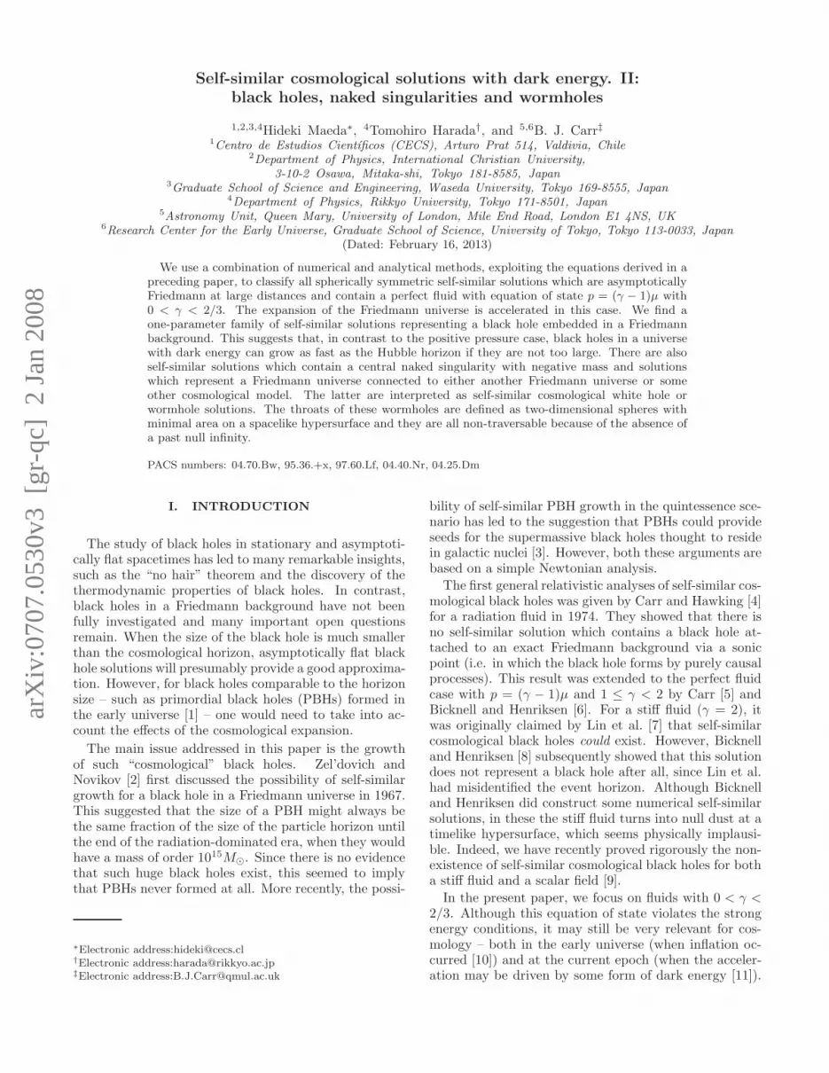
through Eqs. (I.3.11) and (I.3.12). A single free parame-ter A0 then characterizes these solutions. A0 representsthe deviation of the energy density from that of the Fried-mann universe at spatial infinity, with positive (negative)A0 corresponding to an overdensity (underdensity) there.We assume γ = 1/3 as a typical example and numericallyintegrate the ODEs using the constraint equation (I.2.31)or (I.2.32) to monitor the numerical accuracy.
As shown in Paper I, some of the solutions admit anextension beyond z = ∞ (which corresponds to a finitenon-zero physical distance). To assure this, we choosesuitable dependent variables and then expand these asTaylor series with respect to a new independent vari-able around z = ±∞. Paper I specifies the variableswhich satisfy this requirement for asymptotically quasi-Kantowski-Sachs and quasi-static solutions. This is ourkey technique for obtaining the extension of the solu-tion while retaining good numerical accuracy. In orderto display the solutions, we plot −1/z on the horizon-tal axis. The slightly different set of equations used byHarada and Maeda [25] are equivalent to those given inPaper I. In fact, we have constructed numerical codesto evolve both sets of ODEs independently and find ex-cellent agreement. Our numerical accuracy is checkedby the constraint equation, which is always satisfied towithin a factor of 10−7.
We show the numerical solutions in Figs. 1–5. Al-though we have used many other values for the parame-ter A0, we only show the results for A0 = −0.1, −0.08,−0.06, −0.0404, −0.03, −0.02, −0.01, 0, 0.01 and 0.02.A0 = 0 corresponds to the exact Friedmann solution.
Figure 1 shows the velocity function V . The thick linecorresponds to the exact Friedmann solution and thishas one similarity horizon. The solutions with positiveA0 also have one similarity horizon (where V = 1) andencounter curvature singularities with negative mass atfinite positive z, with V converging to 1 from below. Thesolutions with −0.0253 . A0 < 0 have two similarityhorizons and encounter curvature singularities with posi-tive mass at finite negative z, with V converging to 1 fromabove. The solutions with −0.0780 . A0 . −0.0253 also
0
0.5
1
1.5
2
-1 -0.5 0 0.5 1
V
−1/z
0.020.01
0-0.01-0.02-0.03
-0.0404-0.06-0.08-0.1
FIG. 1: V is plotted against −1/z for γ = 1/3. The thick linecorresponds to the exact Friedmann solution (A0 = 0), whichhas one similarity horizon.
have two similarity horizons. However, of these only thesolution with A0 ≃ −0.0404 converges to the asymptoti-cally Friedmann solution as z → 0−; the other solutionsare asymptotically quasi-Friedmann. The solutions withA0 . −0.0780 encounter curvature singularities with pos-itive mass at finite negative z, with V converging to1 from above. The number of similarity horizons de-pends on the value of A0: there are zero, one and twosimilarity horizons for A0 . −0.108, A0 ≃ −0.108 and−0.108 . A0 . −0.0780, respectively.
Figure 2 shows the functions W = 8πGµr2 andW/z2 = 8πGµt2. The thick line W/z2 = 12 correspondsto the exact Friedmann solution (A0 = 0) and has abig-bang singularity as z → +∞ and t → 0. W/z2
diverges at finite positive z for solutions with positiveA0, corresponding to the negative-mass curvature sin-gularities seen above. It also diverges at finite negativez for solutions with −0.0253 . A0 < 0, correspondingto the positive-mass singularities. The solutions with−0.0780 . A0 . −0.0253 have no singularity in W/z2;instead they converge to 12 as z → 0−, corresponding tothe asymptotically quasi-Friedmann solutions.
Figure 3 shows the functions S = R/r and zS. Notethat decreasing (increasing) S as a function of −1/zmeans that the spacetime is expanding (collapsing). Thethick line z2S = 1 corresponds to the exact Friedmannsolution. The curvature singularity at finite non-zero zin the solution with A0 & −0.0253 is a central singular-ity. There exists a collapsing region near this curvaturesingularity in the solution with −0.0253 . A0 < 0. Bycontrast, there exists a single local minimum in the pro-file of zS for the solution with A0 . −0.0253 and thiscorresponds to a wormhole throat. The solution with−0.0780 . A0 . −0.0253 has two different spacelike in-finities at z = 0+ and 0−, where zS diverges to +∞. Thesolution with A0 . −0.0780 also has two different space-

4
20
40
60
80
100
120
140
160
180
200
-0.6 -0.4 -0.2 0 0.2 0.4 0.6
W
−1/z
0.020.01
0-0.01-0.02-0.03
-0.0404-0.06-0.08
-0.1
(a)
0
5
10
15
20
-0.6 -0.4 -0.2 0 0.2 0.4 0.6
W/z
2
−1/z
0.020.01
0-0.01-0.02-0.03
-0.0404-0.06-0.08
-0.1
(b)
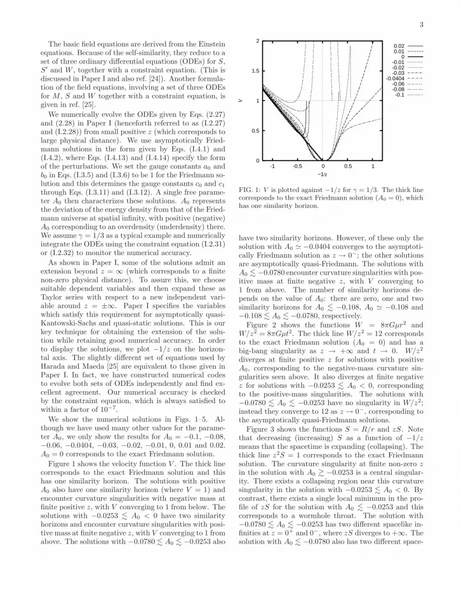
FIG. 2: (a) W = 8πGµr2 and (b) W/z2 = 8πGµt2 are plot-ted against −1/z for γ = 1/3. The thick line W/z2 = 12corresponds to the exact Friedmann solution (A0 = 0).
like infinities at z = 0+ and z = +∞. In the latter class,zS diverges but S is finite, so the solution extends intothe negative z (negative t) region, where S is negativefor positive R.
Figure 4 shows the functions M = 2Gm/r and zM =2Gm/t. The thick line z4M = 4 corresponds to theexact Friedmann solution. We can see that the curva-ture singularity at finite non-zero z in the solutions with−0.0253 . A0 < 0 or A0 . −0.0780 has positive mass,while that in the solution with positive A0 has negativemass. Note that zM is negative for positive m in the so-lutions with A0 . −0.0780, since negative z correspondsto negative t.
Figure 5 shows the function M/S = 2Gm/R. Notethat M/S > 1 and M/S < 1 correspond to the trappedand untrapped regions, respectively, and M/S = 1 in
-0.15
-0.1
-0.05
0
0.05
0.1
0.15
0.2
0.25
0.3
-0.6 -0.4 -0.2 0 0.2 0.4 0.6
S
−1/z
0.020.01
0-0.01-0.02-0.03
-0.0404-0.06-0.08
-0.1
(a)
-0.2
0
0.2
0.4
0.6
0.8
1
-0.6 -0.4 -0.2 0 0.2 0.4 0.6
zS
−1/z
0.020.01
0-0.01-0.02-0.03
-0.0404-0.06-0.08
-0.1
(b)
FIG. 3: (a) S = R/r and (b) zS = R/t are plotted forγ = 1/3. The thick line z2S = 1 corresponds to the exactFriedmann solution (A0 = 0).
the collapsing (expanding) region corresponds to a fu-ture (past) trapping horizon. The thick line correspondsto the exact Friedmann solution; this has a single pasttrapping horizon, corresponding to a cosmological trap-ping horizon. The solutions with positive A0 also have asingle past trapping horizon. Those with A0 . −0.0253have no trapping horizon and the spacetime is trappedeverywhere. Those with −0.0253 . A0 < 0 have one pasttrapping horizon and one future trapping horizon. Thelatter corresponds to a black hole trapping horizon.
From these numerical results, we classify asymptoti-cally Friedmann solutions as z → 0+ into six classes:(a) the flat Friedmann universe (A0 = 0); (b) a cos-mological naked singularity (A0 > 0); (c) a cosmologi-cal black hole (α1 ≤ A0 < 0); (d) a Friedmann-quasi-Friedmann wormhole (α3 < A0 < α1 with A0 6= α2); (e)a Friedmann-Friedmann wormhole (A0 = α2); and (f)
5
-0.2
0
0.2
0.4
0.6
0.8
1
-0.6 -0.4 -0.2 0 0.2 0.4 0.6
M
−1/z
0.020.01
0-0.01-0.02-0.03
-0.0404-0.06-0.08
-0.1
(a)
-2
-1.5
-1
-0.5
0
0.5
1
1.5
2
2.5
-0.6 -0.4 -0.2 0 0.2 0.4 0.6
zM
−1/z
0.020.01
0-0.01-0.02-0.03
-0.0404-0.06-0.08
-0.1
(b)
FIG. 4: (a) M = 2Gm/r and (b) zM = 2Gm/t are plottedfor γ = 1/3. The thick line z4M = 4 corresponds to the exactFriedmann solution (A0 = 0).
a cosmological white hole (A0 < α3). For the presentchoice of gauge constants, α1 ≃ −0.0253, α2 ≃ −0.0404and α3 ≃ −0.0780.
The solutions in class (b) describe a negative massnaked singularity in a Friedmann universe. Those in class(c) describe a positive mass black hole in a Friedmannuniverse. Those in class (d) contain a wormhole throatconnecting a Friedmann universe and a quasi-Friedmannuniverse. Class (e) has only one solution and this con-tains a wormhole throat connecting two Friedmann uni-verses. The solutions in class (f) describe a positive masswhite hole in a Friedmann universe which contains awormhole throat connecting a Friedmann universe anda quasi-static spacelike infinity.
The exact flat Friedmann solution, the only solution ofclass (a), is located at the threshold between classes (b)and (c), while we could not resolve the threshold solution
0
0.5
1
1.5
2
2.5
3
3.5
-0.6 -0.4 -0.2 0 0.2 0.4 0.6
M/S
−1/z
0.020.01
0-0.01-0.02-0.03
-0.0404-0.06-0.08
-0.1
FIG. 5: M/S = 2Gm/R is plotted for γ = 1/3. The thickline corresponds to the exact Friedmann solution (A0 = 0).
between classes (d) and (f). The solution of class (e) isobtained by fine-tuning the parameter A0. We investi-gate their properties and physically interpret them in thenext section.
III. PHYSICAL INTERPRETATION
A. Exact flat Friedmann universe
z=
z1
z = +0, t = ∞
z=
z 1, t
=0
z=
∞,r
=∞
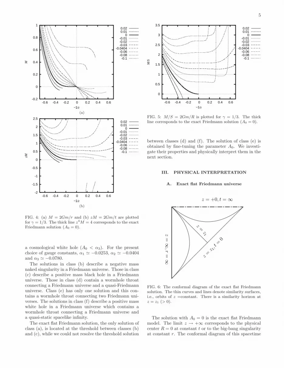
FIG. 6: The conformal diagram of the exact flat Friedmannsolution. The thin curves and lines denote similarity surfaces,i.e., orbits of z =constant. There is a similarity horizon atz = z1 (> 0).
The solution with A0 = 0 is the exact flat Friedmannmodel. The limit z → +∞ corresponds to the physicalcenter R = 0 at constant t or to the big-bang singularityat constant r. The conformal diagram of this spacetime

6
z=z1Friedmann
infinity
FIG. 7: The t-r plane of the exact flat Friedmann solution.A fluid element moves from the bottom to the top. r = 0 andr → +∞ correspond to spacelike infinity and the physicalcenter (R = 0), respectively. t = 0 corresponds to the big-bang singularity, which is represented by a zig-zag line. Thereis a similarity horizon at z = z1 (> 0), corresponding to acosmological event horizon.
and the t-r plane of the solution are shown in Figs. 6 and7, respectively. There is a similarity horizon at z = z1,where V = 1, corresponding to the cosmological eventhorizon and the initial singularity is null.
B. Cosmological naked singularity
z=
z1
z=
z∗
z = +0, t = ∞
z=
z 1, t
=0
FIG. 8: The conformal diagram of the cosmological nakedsingularity solution. There is a similarity horizon at z = z1
(> 0). z = z∗ (> 0) with 0 < t < ∞ corresponds to a timelikesingularity at which the mass is negative.
The solutions with A0 > 0 represent asymptoticallynegative-mass singularities as z → z∗ (0 < z∗ < ∞).
z=z*
z=z1
Friedmanninfinity
FIG. 9: The t-r plane of the cosmological naked singular-ity solution. r = 0 corresponds to spacelike infinity. Thereis a similarity horizon at z = z1 (> 0), corresponding to acosmological event horizon. z = z∗ (> 0) with 0 < t < ∞
corresponds to a timelike singularity of negative mass and isrepresented by a zigzag line.
From Fig. 3, we see that R,r > 0 everywhere and alsoR,t > 0 (i.e. the spacetime is expanding), where a commadenotes a partial derivative. Figures 1 and 5 show thatthere is a cosmological event horizon and a cosmologicaltrapping horizon. Near the singularity, V approaches 1from below according to Eq. (I.4.60) with negative V1.Figures 4 and 5 show that the singularity has negativemass and is in the untrapped region. This solution de-scribes a naked singularity embedded in a Friedmannbackground. The conformal diagram of the spacetimeand the t-r plane of the solution are shown in Figs. 8 and9, respectively. There is a similarity horizon at z = z1
and this corresponds to the cosmological event horizon.
C. Cosmological black hole
The solutions with α1 ≤ A0 < 0 (α1 ≃ −0.0253)are asymptotically quasi-Kantowski-Sachs as z → ±∞and asymptotically positive-mass singular as z → z∗(−∞ < z∗ < 0). Because the solutions are asymptoti-cally quasi-Kantowski-Sachs as z → +∞, they can be ex-tended analytically into the region with negative z. Sincethe Kantowski-Sachs solution has a curvature singularityat t = 0, the analytic extension in this case must be in-terpreted as an extension from the positive r to negativer region. In the extended region, S and M are negativebut the areal radius R = rS and mass m = rM/(2G) arepositive because r is negative.
From Fig. 3, we find that R,r > 0 holds everywhereand there exists a collapsing region (with R,t < 0) nearthe singularity. It is seen in Fig. 5 that there are twotrapping horizons, one in the expanding region and theother in the collapsing region. These are the cosmological

7
and black hole trapping horizons, respectively. Figure 10shows that the trapping horizon is degenerate for the crit-ical value A0 = α1. Figures 1 or 10 show that there isboth a cosmological and black hole event horizons. ForA0 = −0.01 and −0.02, we see that the black hole andcosmological event horizons are in the untrapped andtrapped regions, respectively. Near the singularity, Vapproaches 1 from above according to Eq. (I.4.60) withpositive V1. Figures 4 and 5 show that the singularityhas positive mass and is in the trapped region.
The forms of zS = R/t for the various horizons areplotted as functions of the parameter A0 in Fig. 11. Theratio of the black hole event horizon size to the cosmo-logical event horizon size goes from 0 to 0.36, while theratio of the black hole event horizon size to the back-ground Hubble horizon size goes from 0 to 0.70. On theother hand, the ratio of the cosmological trapping hori-zon size to the black hole trapping horizon size goes from0 to roughly 1.
This solution describes a black hole in a Friedmannbackground. Figures 12 and 13 show the conformal dia-gram and t-r plane for the cosmological black hole solu-tion. We can see that the initial singularity is null andthat there exists both a null and spacelike portion of theblack hole singularity. There are two similarity horizonsat z1 > 0 and z2 < 0. These correspond to the cosmo-logical and black hole event horizons, respectively.
D. Friedmann-quasi-Friedmann wormhole
The solutions with α3 < A0 < α1 (α3 ≃ −0.0780) arealso asymptotically quasi-Kantowski-Sachs as z → ±∞and the form of these solutions in the extended regioncan again be obtained numerically. Figure 14 shows thatW/z2 → 12 and z2S → constant as z → 0−. In theasymptotically Friedmann case (A0 = α2 ≃ −0.0404)the constant is −1. Otherwise the solutions are asymp-totically quasi-Friedmann as z → 0− and the constant isdifferent from −1.
From the profile of zS in Fig. 3, we see that a solutionin this class has a single throat at z = zt, characterizedby R,r = 0 and R,r < (>)0 for −1/z < (>) − 1/zt, i.e.the areal radius R has a minimum on the spacelike hy-persurface with constant t. As a result, the spacetimerepresents a dynamical wormhole with a throat connect-ing a Friedmann universe to another Friedmann or quasi-Friedmann universe. With A0 = α2, the solution has re-flection symmetry, so the wormhole throat connects twoexact Friedmann universes and is located at z = ±∞.Fine-tuning of A0 is required because the asymptoticallyFriedmann solution given by Eqs. (I.4.13) and (I.4.14) isnon-generic among the solutions of the linearized equa-tions for A, A′, B′ and B′′ in the region where V 2 → ∞(see Paper I).
This wormhole universe is born from the initial singu-larity at t = 0, around which the spacetime for fixed ris described by the quasi-Kantowski-Sachs solution. The
0
0.5
1
1.5
2
0 0.2 0.4 0.6 0.8 1 1.2
V
zS=R/t
-0.001-0.01-0.02
-0.0252
(a)
0
0.5
1
1.5
2
0 0.2 0.4 0.6 0.8 1 1.2
M/S
=2G
m/R
zS=R/t
-0.001-0.01-0.02
-0.0252
(b)
FIG. 10: (a) V and (b) M/S as functions of zS(= R/t) forthe cosmological black hole solutions.
profile of S in Fig. 3 shows that the spacetime is ex-panding everywhere and Fig. 4 shows that it has positivemass. From Figs. 1 and 5, there are two similarity hori-zons, corresponding to two cosmological event horizons,but there is no trapping horizon.
Figures 15 and 16 show the conformal diagram and t-rplane for the Friedmann-quasi-Friedmann wormhole so-lution. We can see that the initial singularity is null andthat there are two parts of future null infinity, both be-ing spacelike and having Friedmann and quasi-Friedmannasymptotics. There are two similarity horizons at z1 > 0and z2 < 0, both corresponding to cosmological eventhorizons. Figure 5 shows that the spacetime is trappedeverywhere, so there is no trapping horizon. This explicitexample shows that the wormhole definitions of Hochbergand Visser [17] or Hayward [18] are too restrictive.

8
0
0.2
0.4
0.6
0.8
1
1.2
1.4
-0.03 -0.025 -0.02 -0.015 -0.01 -0.005 0
zS=
R/t
A0
Cosmological event horizonBlack hole event horizon
Cosmological trapping horizonBlack hole trapping horizon
FIG. 11: The value of zS = R/t for various horizons is plottedas a function of the parameter A0 for the cosmological blackhole solutions with γ = 1/3.
z=
z1z
=z 2
z = z∗
z = +0, t = ∞
z=
z 1, t
=0
z=
±∞
,r
=±∞
z=
z2 , t
=0
FIG. 12: The conformal diagram of the cosmological blackhole solution. There are two similarity horizons at z = z1
and z = z2 (z2 < 0 < z1). z = z1 with 0 < t < ∞ is thecosmological event horizon, while z = z2 with 0 < t < ∞ isthe black hole event horizon. z = z∗ (< 0) with 0 < t < ∞
gives a spacelike singularity with positive mass.
Friedmann
z=z1
z=z*
z=z2
infinity
FIG. 13: The t-r plane of the cosmological black hole solution.r = 0+ corresponds to spacelike infinity.
0
5
10
15
20
-2 -1 0 1 2 3 4 5
W/z
2
−1/z
0.020.01
0-0.01-0.02-0.03
-0.0404-0.06-0.08
-0.1
(a)
-2
-1.5
-1
-0.5
0
0.5
1
1.5
-2 -1.5 -1 -0.5 0 0.5 1 1.5 2
z2S
−1/z
0.020.01
0-0.01-0.02-0.03
-0.0404-0.06-0.08
-0.1
(b)
FIG. 14: (a) W/z2 and (b) z2S are plotted for γ = 1/3.
E. Cosmological white hole
The solutions with A0 < α3 are asymptotically quasi-static as z → ±∞, so that S = R/r converges to a con-stant there (see Fig. 3). We can therefore extend themanalytically into the negative z region, which correspondsto negative t.
The variables S and W can be used to obtain the solu-tions in the extended region because they are finite in theasymptotically quasi-static solutions at z = ±∞. In theextended region, zS and zM are negative but the arealradius R = rS and mass m = rM/(2G) are positive be-cause t is negative.
The profile of zS = R/t in Fig. 3 shows that its min-imum value corresponds to a throat connecting a flatFriedmann infinity and a quasi-static infinity, so this de-scribes a dynamical wormhole. The spacetime is expand-ing everywhere and has positive mass from Fig. 4. Fig-

9
PSfrag
z=
z1z
=z 2
z = +0, t = ∞z = −0, t = ∞
z=
z 1, t
=0
z=
±∞
,r
=±∞
z=
z2 , t
=0
FIG. 15: The conformal diagram of the Friedmann-quasi-Friedmann wormhole solution. There are two similarity hori-zons, z = z1 and z = z2 (z2 < 0 < z1), both corresponding tocosmological event horizons. z = 0+ and z = 0− give twodistinct null infinities, described by Friedmann and quasi-Friedmann asymptotics, respectively. z = ±∞, however, isdescribed by the Kantowski-Sachs asymptotic as t increasesfrom 0 to ∞.
z=z1z=z2
z=zt
Friedmanninfinity (r=+0)
Quasi-Friedmanninfinity (r=-0)
FIG. 16: The t-r plane of the Friedmann-quasi-Friedmannwormhole solution. We show the solution with a wormholethroat at z = zt in the positive z region. r = 0+ and 0−
correspond to the Friedmann and quasi-Friedmann infinities,respectively. t = 0 corresponds to the big-bang singularity,represented by the quasi-Kantowski-Sachs solution.
ure 5 shows that it is trapped everywhere, so there is notrapping horizon.
As seen in Figs. 2 and 3, there is a central curvaturesingularity at z = z∗ in the negative z region and themass is positive there from Fig. 4. This corresponds tothe singular positive-mass asymptote discussed in PaperI. Near the singularity, V is approximated by Eq. (I.4.60)with positive V1 and approaches 1 from Fig. 1. The sin-gularity is spacelike because of the positive mass and re-sembles a Schwarzschild white hole singularity (althoughthere is no trapping horizon). This singularity is non-simultaneous, so it differs from the big-bang singularity.On the other hand, the singularity at t = 0 with z = z1
is massless and does correspond to the big-bang singular-ity. The solution describes a white hole in the Friedmann
universe.As seen in Fig. 1, the solutions can be classified into
three types, according to whether they have no similar-ity horizon (A0 ≤ α4), one degenerate similarity hori-zon (A0 = α4) or two non-degenerate similarity horizons(α4 < A0 < α3), where α4 ≃ −0.108. The degeneratecase is obtained by fine-tuning A0.
Figures 17 and 18 show the conformal diagram and t-r plane for these three types of Friedmann-quasi-staticwormhole solutions. In the case with similarity hori-zon(s), the singularity has both spacelike and null por-tions, which correspond to the white hole and initial sin-gularities, respectively, and there are two parts of futurenull infinity. One is spacelike and described by the Fried-mann asymptote and the other is null. In the case withno similarity horizon, the singularity and future null in-finity are both spacelike.
In closing this section, a comment should be madeabout what is meant by the term “wormhole”. It issometimes assumed that wormholes require negative en-ergy density and there are certainly theorems to this ef-fect [17, 18, 19]. Our solutions do not require negativeenergy density but this does not conflict with these theo-rems because we have a different definition of a wormholethroat.
The theorems claiming the violation of the null energycondition at a wormhole throat [17, 18] define the throaton a null hypersurface. In this case, the throat coincideswith a trapping horizon. In the present paper we definea wormhole throat on a spacelike hypersurface. In fact,our wormhole solutions do not have a trapping horizon atall, so they are not wormholes in the sense of Hochbergand Visser [17] or Hayward [18] even though they possesstwo distinct infinities. We discuss this problem in a moregeneral framework in a separate paper [26].
Here we also consider the threshold between theFriedmann-quasi-Friedmann solutions and the cosmolog-ical white hole solutions. Strictly speaking, the thresholdsolution with the exact parameter value A0 = α3 cannotbe achieved numerically. Among the asymptotic solu-tions obtained in Paper I, the constant-velocity asymp-tote will be the most plausible candidate for this thresh-old solution. The resulting conformal diagram would begiven by Fig. 19, admitting a null ray traveling from theconstant velocity infinity (z → +∞, r → +∞) to theFriedmann infinity (z → +0, t → ∞). However, this pos-sibility is clearly excluded because this diagram containsa traversable dynamical wormhole, which is prohibitedby the discussion in Hochberg and Visser [17] or Hay-ward [18].
IV. SUMMARY AND DISCUSSION
We have numerically investigated spherically symmet-ric self-similar solutions for a perfect fluid with p =(γ − 1)µ (0 < γ < 2/3) which are properly asymptotic to

10
z = z∗
z = +0, t = ∞
z = ±∞, t = ±0
(a)
PSfrag
z=
z1
z = z∗
z = +0, t = ∞
z=
z 1, t
=0
z=
z 1, t
=∞
z = ±∞, t = ±0
(b)
z=
z1
z=
z2
z = z∗
z = +0, t = ∞
z=
z 1, t
=0
z = ±∞, t = ±0
z=
z 2, t
=∞
(c)
FIG. 17: The conformal diagrams of the cosmological whitehole solutions with: (a) no similarity horizon; (b) one degen-erate similarity horizon z = z1 (> 0); and (c) two distinctsimilarity horizons z = z1 and z = z2 (0 < z1 < z2 < ∞). Foreach case, z = z∗ (< 0) is a spacelike singularity with positivemass. In (b), z = z1 with t = ∞ corresponds to future nullinfinity. In (c), z = z2 with t = ∞ corresponds to future nullinfinity.
the flat Friedmann model at large distances, in the sensethat there is no solid angle deficit. We have integratedthe field equations for the self-similar solutions and in-terpreted the solutions using the asymptotic analysis ofPaper I. The results are summarized in Table I.
We have seen that there is a class of asymptoticallyFriedmann self-similar black hole solutions and this con-trasts to the situation with positive pressure fluids orscalar fields, where there are no such solutions. Thissuggests that self-similar growth of PBHs is possible inan inflationary flat Friedmann universe with dark energy,which may support the claim in ref. [3]. This can be ex-plained by the fact that the pressure gradient of darkenergy is in the opposite direction to the density gradi-ent. It therefore gives an attractive force which pulls thematter inwards, whereas the gravitational force is repul-
z=zt
z=z*
Friedmanninfinity
FIG. 18: The t-r plane of the cosmological white hole solu-tion in the case without a similarity horizon. r = 0+ and+∞ correspond to the Friedmann and quasi-static infinities,respectively. There is a wormhole throat at z = zt in thepositive z region. z = z∗ (< 0) with 0 < t < ∞ correspondsto a spacelike singularity with positive mass, represented bya zigzag line.
z=
z1
z = +0, t = ∞
z=
z 1, t
=0
z=
∞,r
=∞
FIG. 19: The fictitious conformal diagram of the Friedmann-constant-velocity wormhole solution. There is a similarityhorizon at z = z1 (> 0), corresponding to the cosmologicalevent horizon. z = ∞ with 0 < t < ∞ corresponds to atimelike boundary of spacetime at infinity.
sive. So if the black hole is small and the density gradientsteep, it can accrete the surrounding mass effectively.
For γ = 1/3, we have found numerically that the ratioof the size of the black hole event horizon to the Hubblelength is between 0 and 0.70. This means that the size ofsuch a self-similar cosmological black hole has an upperlimit but it can be arbitrarily small, so black holes which

11
TABLE I: Self-similar solutions with γ = 1/3 which areasymptotic to a Friedmann universe at large distance. Thenumerical values are given by α1 ≃ −0.0253, α2 ≃ −0.0404,α3 ≃ −0.0780 and α4 ≃ −0.108 for the choice of the gaugeconstants a0 = b0 = 1. The terms similarity horizon,trapping horizon, Friedmann, quasi-static, quasi-Kantowski-Sachs, positive-mass singular, negative-mass singular are ab-breviated as SH, TH, F, QS, QKS, PMS and NMS, respec-tively. The last two columns give the number of similarityand trapping horizons, with 1(d) indicating one degeneratehorizon. We note that the spacetime for A0 = α3 has notbeen determined.
A0 Spacetime Asymptote # SH # TH
Naked singularity F-NMS 1 1
0 Friedmann universe F 1 1
Black hole F-QKS-PMS 2 2
α1 Black hole F-QKS-PMS 2 1 (d)
Wormhole F-QKS-QF 2 0
α2 Wormhole F-QKS-F 2 0
Wormhole F-QKS-QF 2 0
α3 ? ? ? ?
White hole F-QS-PMS 2 0
α4 White hole F-QS-PMS 1(d) 0
White hole F-QS-PMS 0 0
grow as fast as the universe cannot be too large. It shouldbe stressed that there is a one-parameter family of self-similar cosmological black hole solutions, so we do nothave to fine-tune the mass of the black hole to get self-similar growth. This means that self-similar black holegrowth is very plausible in a universe with dark energyof this kind. This is in contrast to the usual Newtonianargument for a positive pressure fluid [2, 20].
In addition to the black hole solutions, we have foundself-similar solutions which represent a Friedmann uni-verse connected to either another Friedmann universe orsome other cosmological model. They are interpretedas self-similar cosmological white hole or wormhole so-lutions. These are classified into three types, accord-ing to whether the other infinity is Friedmann, quasi-Friedmann, or quasi-static, among which the last type isinterpreted as a white hole in a Friedmann background.
These solutions provide intriguing examples of dynam-ical wormholes. Since they are cosmological solutions,they are not asymptotically flat and they do not havea regular past null infinity. Rather they are asymptoticto models which are expanding at spacelike infinity andhave an initial singularity.
In such situations a wormhole throat should be locallydefined as a two-sphere of minimal area on the spacelikehypersurfaces rather than a trapping horizon. Accordingto the conventional definition of traversability, none ofour numerical solutions represents a traversable worm-hole because of the absence of a past null infinity. Thestrong energy condition is violated there but the null,dominant and weak energy conditions are still all sat-isfied. Our wormhole solutions do not have a trappinghorizon: because there is no violation of the null energycondition, they are not dynamical wormholes in the senseof Hochberg and Visser [17] or Hayward [18].
Finally, we note that the homothetic (rather than co-moving) approach is another powerful method of study-ing self-similar solutions. In the positive pressure case,the homothetic and comoving approaches are comple-mentary, which leads to a comprehensive understandingof self-similar solutions [24, 27, 28]. A dynamical systemsapproach in the negative pressure case should also shedlight on various aspects of the problem.
Acknowledgments
The authors would like to thank S.A. Hayward,P. Ivanov, H. Kodama, H. Koyama, M. Siino andT. Tanaka for useful comments. HM and TH are sup-ported by the Grant-in-Aid for Scientific Research Fundof the Ministry of Education, Culture, Sports, Scienceand Technology, Japan (Young Scientists (B) 18740162(HM) and 18740144 (TH)). BJC thanks the ResearchCenter for the Early Universe at the University of Tokyofor hospitality received during this work. HM was alsosupported by the Grant No. 1071125 from FONDECYT(Chile). CECS is funded in part by an institutional grantfrom Millennium Science Initiative, Chile, and the gener-ous support to CECS from Empresas CMPC is gratefullyacknowledged.
[1] S.W. Hawking, Mon. Not. R. Astron. Soc. 152, 75 (1971).[2] Ya.B. Zel’dovich and I.D. Novikov, Sov. Astron. A. J. 10,
602 (1967).[3] R. Bean and J. Magueijo, Phys. Rev. D66, 063505 (2002).[4] B.J. Carr and S.W. Hawking, Mon. Not. R. Astron. Soc.
168, 399 (1974).[5] B.J. Carr, Ph.D. thesis, Cambridge University (1976).[6] G.V. Bicknell and R.N. Henriksen, Astrophys. J. 219,
1043 (1978).[7] D. Lin, B.J. Carr, and S.M. Fall, Mon. Not. R. Astron.
Soc. 177, 51 (1976).[8] G.V. Bicknell and R.N. Henriksen, Astrophys. J. 219,
1043 (1978).[9] T. Harada, H. Maeda, B.J. Carr, Phys. Rev. D74, 024024
(2006).[10] A.D. Linde, Particle Physics and Inflationary Cosmol-
ogy (Harwood Academic Publishers, Chur, Switzerland1990).
[11] S. Perlmutter et al., Astrophys. J. 517, 565 (1999);A.G. Riess et al., Astron. J. 116, 1009 (1998); Astron. J.

12
117, 707 (1999).[12] E. Babichev, V. Dokuchaev, Yu. Eroshenko, Phys. Rev.
Lett. 93, 021102 (2004).[13] E. Babichev, V. Dokuchaev, Yu. Eroshenko, J. Exp.
Theor. Phys. 100, 528 (2005).[14] A. Nusser, Mon. Not. R. Astron. Soc. 375, 1106 (2007).[15] H. Maeda, J. Koga and K-i. Maeda, Phys. Rev. D66,
087501 (2002).[16] M.S. Morris and K.S. Thorne, Am. J. Phys. 56, 395
(1988).[17] D. Hochberg and M. Visser, Phys. Rev. D58, 044021
(1998).[18] S.A. Hayward, Int. J. Mod. Phys. D8, 373 (1999).[19] M. Visser, Lorentzian Wormholes: From Einstein to
Hawking, (Springer-Verlag, Berlin, Germany, 1997).
[20] T. Harada and B.J. Carr, Phys. Rev. D72, 044021 (2005).[21] T. Harada, H. Maeda and B.J. Carr, arXiv:0707.0528
[gr-qc], to appear in Physical Review D (Paper I).[22] S.A. Hayward, Phys. Rev. D49, 6467 (1994).[23] S.A. Hayward, Phys. Rev. D53, 1938 (1996).[24] B.J. Carr and A.A. Coley, Phys. Rev. D62, 044023
(2000).[25] T. Harada and H. Maeda, Phys. Rev. D63, 084022
(2001).[26] H. Maeda, T. Harada and B.J. Carr, in preparation.[27] M. Goliath, U.S. Nilsson and C. Uggla, Class. Quant.
Grav. 15, 167; ibid. 2841 (1998).[28] B.J. Carr, A.A. Coley, M. Goliath, U.S. Nilsson and C.
Uggla, Class. Quant. Grav. 18, 303 (2001).


