Embed Size (px)
Citation preview

Daniele Gorla
Semantic Approaches toGlobal Computing Systems
PhD ThesisDottorato in Informatica ed Applicazioni, ciclo XVII
Dipartimento di Sistemi ed Informatica
Universita degli Studi di Firenze
Advisors:
Prof. Rocco De Nicola
Prof. Rosario Pugliese
International Reviewers: Members of the Jury:
Dr. Gerard Boudol Prof. Pierluigi Crescenzi
Prof. Michele Bugliesi Prof. Roberto Grossi
Prof. Davide Sangiorgi
Date of submission: December 31, 2004
Date of defence: February 15, 2005

2

3
Abstract
Programming computational infrastructures available globally for offering uni-form services has become one of the main issues in Computer Science. The chal-lenges come from the variable guarantees for communication, co-operation andmobility, resource usage, security policies and mechanisms, etc. that have to betaken into account. A key issue is the definition of innovative theories, compu-tational paradigms, linguistic mechanisms and implementation techniques for thedesign, realisation, deployment and management of global computational environ-ments and their application.
A successful contribution to this research line is K, an experimental lan-guage with primitives for programming global computers that combines the pro-cess algebra approach with the coordination-oriented one. Its main features areprocess distribution and mobility, remote operations and asynchronous communi-cation via multiple distributed tuple spaces. K has proved to be suitable forprogramming a wide range of distributed applications with agents and code mobil-ity, and has been implemented on the top of a runtime system written in Java.
In this thesis, we first presents some foundational calculi for mobility basedon K. Then, we concentrate on one of these calculi, namely µK, that re-tains most of the peculiar features of K, while being much simpler. We presenttwo approaches to study the behaviours of global computing systems expressed inµK: (non-standard) type systems and behavioural equivalences. Type systemspermit to control resource accesses, as well as data and process movements. Be-havioural equivalences, on the other hand, permit to state and verify properties ofdistributed applications. Finally, we focus on the expressive power of the calculi byproviding encodings of each calculus into a simpler one. The overall expressive-ness is then assessed via a formal comparison with the asynchronous π-calculus.

4

5
Acknowledgements
In the years of my PhD, I had the luck of being supervised by Rocco De Nicolaand Rosario Pugliese. Apart from their scientific support, that was really enor-mous, I could also benefit from their friendship, humanity and honesty. Theirexperience and their suggestions taught me the way theorems can be proved but,mainly, gave me the enthusiasm of pursuing research. I wish their teachings willalways remain fixed in my mind. Rocco also allowed me to work in the group ofFlorence, while living in Rome: this was extremely important for me and for myfamily.
I am also incredibly indebted with Anna Labella, my MS supervisor. Herfriendship and her support are at the basis of my PhD: she introduced me to Roccoand she always engaged me in collaborations at the Department of Informatics ofthe University of Rome “La Sapienza”. I also thank the deans of this departmentfor the office given me in these years.
My research benefited from the collaborations with several, first-class authors.A part from Rocco and Rosario, I mention (in alphabetical order) Michele Bore-ale, Chiara Braghin, Matthew Hennessy, Anna Labella, Vladimiro Sassone and theConcurrency and Mobility Group in Florence. Most of the work carried on withthem does not appear in this thesis; however, it strongly influenced all my research.In particular, Michele introduced me the field of semantics, while Matthew andVladimiro very friendly hosted me in the Department of Informatics of the Univer-sity of Sussex (Brighton, UK). Moreover, I also benefited from several discussionswith a lot of people: Cedric Fournet (that kindly hosted me at Microsoft Research,Cambridge – UK), Jose Fiadeiro, Antonia Lopez and all the researchers involvedin the projects we were part of.
I am very grateful to Gerard Boudol and Michele Bugliesi that referred thisthesis. Their constructive attitude and the time they spent on these pages produceda lot of precious suggestions that improved the quality of my work. I also thankthe members of my PhD jury for their efforts aimed at evaluating my work.
My research and my personal education required a lot of money, that wereprovided by several companies and institutions. First of all, I really thank theMicrosoft Research at Cambridge (UK) that financed my PhD grant within theproject NAPI. In these years, I had the opportunity to attend several conferences,schools and meetings. The money I spent were kindly provided by the EU andby the Italian MURST by means of several research projects: Agile (EU-FET-GC, Contract IST-2001-32747), Mikado (EU-FET-GC, Contract IST-2001-32222),TOSCA (MURST-Cofin) and NAPOLI (MURST-Cofin). The EU also paid my stayat Brighton in the summer 2003 with a Marie Curie fellowship.

6
Last but not least, I cannot describe the impact of my family in my work. Myparents always supported my education with their love (and their money) and al-ways encouraged me to take my own choices. My mother was a fundamentalpresence in our home and helped us even when her health suggested a rest. Mychildren, Martina and Niccolo, filled my life of joy. Finally, my wife Monica is theessence of my happiness: she gave me the strength to react against the difficultiesof everyday life, she had the patience of bearing me and she was always the firstsupporter of my works. This thesis is dedicated to all of them.

Contents
1 Introduction 91.1 Global Computers . . . . . . . . . . . . . . . . . . . . . . . . . . 91.2 Formal Methods for Global Computers . . . . . . . . . . . . . . . 111.3 The Language K . . . . . . . . . . . . . . . . . . . . . . . . 131.4 Overview of the thesis . . . . . . . . . . . . . . . . . . . . . . . 15
2 A Family of Process Languages 172.1 K . . . . . . . . . . . . . . . . . . . . . . . . . . . . . . . . 172.2 µK: micro K . . . . . . . . . . . . . . . . . . . . . . . . 222.3 K: core K . . . . . . . . . . . . . . . . . . . . . . . . . 232.4 K: local core K . . . . . . . . . . . . . . . . . . . . . 232.5 Related Work: Languages for GCs . . . . . . . . . . . . . . . . . 24
3 Types to Control Process Activities 293.1 Overview: the Approach and Key Principles . . . . . . . . . . . . 303.2 A Basic Type System . . . . . . . . . . . . . . . . . . . . . . . . 32
3.2.1 Static Semantics . . . . . . . . . . . . . . . . . . . . . . 323.2.2 Dynamic Semantics . . . . . . . . . . . . . . . . . . . . 343.2.3 Type Soundness . . . . . . . . . . . . . . . . . . . . . . 37
3.3 Dynamic Management of Capabilities . . . . . . . . . . . . . . . 413.3.1 Language Semantics . . . . . . . . . . . . . . . . . . . . 433.3.2 Type Soundness . . . . . . . . . . . . . . . . . . . . . . 473.3.3 Example: Subscribing On-line Publications . . . . . . . . 503.3.4 Variations on Capability Management . . . . . . . . . . . 523.3.5 Discussion on Capability Management . . . . . . . . . . 63
3.4 Fine-grained Controls on Process Activities . . . . . . . . . . . . 653.4.1 Fine-grained Types . . . . . . . . . . . . . . . . . . . . . 653.4.2 Static Semantics . . . . . . . . . . . . . . . . . . . . . . 683.4.3 Dynamic Semantics and Type Soundness . . . . . . . . . 693.4.4 Example: A Bank Account Management System . . . . . 73
3.5 Related Work . . . . . . . . . . . . . . . . . . . . . . . . . . . . 75
7

8 CONTENTS
4 Types for Confining Data and Processes 794.1 Controlling Data Movement via Types . . . . . . . . . . . . . . . 804.2 Static Inference and Checking . . . . . . . . . . . . . . . . . . . 814.3 Typed Operational Semantics . . . . . . . . . . . . . . . . . . . . 854.4 Type Soundness . . . . . . . . . . . . . . . . . . . . . . . . . . . 874.5 Example: Implementing a Multiuser System . . . . . . . . . . . . 914.6 Discussion and Related Work . . . . . . . . . . . . . . . . . . . . 96
5 Behavioural Theories 995.1 Touchstone Equivalences . . . . . . . . . . . . . . . . . . . . . . 1005.2 Bisimulation Equivalence . . . . . . . . . . . . . . . . . . . . . . 104
5.2.1 Soundness w.r.t. Barbed Congruence . . . . . . . . . . . 1075.2.2 Completeness w.r.t. Barbed Congruence . . . . . . . . . . 113
5.3 Trace Equivalence . . . . . . . . . . . . . . . . . . . . . . . . . . 1175.3.1 Soundness w.r.t. May Testing . . . . . . . . . . . . . . . 1205.3.2 Completeness w.r.t. May Testing . . . . . . . . . . . . . . 123
5.4 Verifying a Protocol for the Dining Philosophers . . . . . . . . . . 1295.5 Equational Laws and the Impact of Richer Contexts . . . . . . . . 1325.6 Related Work . . . . . . . . . . . . . . . . . . . . . . . . . . . . 134
6 Expressiveness of the Languages 1376.1 Technical Preliminaries . . . . . . . . . . . . . . . . . . . . . . . 1386.2 K vs µK . . . . . . . . . . . . . . . . . . . . . . . . . . 1406.3 µK vs K . . . . . . . . . . . . . . . . . . . . . . . . . . 1496.4 K vs K . . . . . . . . . . . . . . . . . . . . . . . . . 1596.5 A Comparison with the πa-calculus . . . . . . . . . . . . . . . . . 163
6.5.1 Encoding the πa-calculus in K . . . . . . . . . . . . 1646.5.2 Encoding K in the πa-calculus . . . . . . . . . . . . 169
6.6 Concluding Assessment and Related Work . . . . . . . . . . . . . 172
7 Conclusion and Future Work 177
A Symbols and Notations 179

Chapter 1
Introduction
Technological advances of both computers and telecommunication networks, anddevelopment of more efficient communication protocols are leading to a ever-increasing integration of computing systems and to diffusion of the so called globalcomputer (GC, for short). This is a massive networked and dynamically recon-figurable infrastructure interconnecting heterogeneous, typically autonomous andmobile components, that can operate on the basis of incomplete information.
A key research challenge is to devise theoretical models and calculi with a for-mal semantics for specifying, programming and reasoning about global computingsystems. These calculi could provide a sound basis for constructing GCs which are“sound by construction” and which behave in a predictable and analysable man-ner. The crux is to identify what abstractions are more appropriate and to supplyfoundational and effective tools to support development and certification (statingand proving correctness) of global computing applications. This thesis aims atpresenting a fully accounted work along this direction.
Before starting with the technical details, we shall carry on a more exhaustivediscussion about the key features of GC and describe the state-of-the-art in thisfield. A summary of the thesis is given at the end of this chapter.
1.1 Global Computers
GC merge the features of traditional distributed systems together with the featuresof open systems. They borrow from distributed systems the intrinsic concurrency,the distribution of components, the absence of a global state and the asynchronyin changes of local states. They borrow from open systems the possibility fornew entities (usually called agents or processes) of dynamically enter and exit thesystem, the heterogeneity and autonomy of components, the dynamic change ofsystem configuration and the mobility of programs/data.
Applications for GC distinguish themselves from traditional distributed appli-cations in terms of scalability (huge number of users and nodes), connectivity (bothavailability and bandwidth), heterogeneity (of operating systems and application
9

10 CHAPTER 1. INTRODUCTION
software), autonomy (of administration domains and mobile agents), and, mostly,in terms of the ability of dealing with dynamic and unpredictable changes of theirnetwork environment (e.g. availability of network connectivity, lack of resources,node failures, network reconfigurations and so on). GC are fostering a new style ofdistributed programming whose key principle is network awareness: applicationsnow have information on network settings and can adapt to their variation. Indeed,applications often need to be aware of the administrative domains where they arecurrently located, and need to know how to cross administrative boundaries or howto access remote resources. Moreover, distant communication and use of remoteresources is also affected, e.g., by the physical distance between locations and bycongestion or (temporary/permanent/intermittent) failure of the underlying com-munication network [34].
The explicit introduction of locations in the picture imposes some sensible pro-gramming choices. Indeed, locations are abstractions for components (i.e., pro-cesses or resources) which share some interface with the environment. The kind ofthis interface may be, however, of various nature. For example, one can considerlocations as units of communication (i.e. they provide address spaces for inter-processes exchanges), units of migration (i.e. co-located components move as awhole), units of failure (i.e. co-located components fail as a whole), units of secu-rity (i.e. co-located components share a security policy), and so on. Thus, everylanguage for GCs must clarify the intended meaning assigned to locations; usually,the constructs of the language are then tailored accordingly.
The explicit knowledge of the distributed framework underlying a GC leadsto another relevant consideration: programmers can refer localities when writingtheir programs. This fact requires the introduction in the language of constructsto deal with network awareness. Moreover, such constructs should be simple andpowerful, while respecting the underlying meaning assigned to localities.
A suitable abstraction to design and program network-aware applications ismobility. Its usefulness emerges when developing applications that can implementboth processes moving across the net to run over different hosts (mobile computa-tion) and mobile devices with intermittent access to the network (mobile comput-ing). In the literature, the term mobility is used to denote different mechanisms,ranging from simple ones (e.g., downloading of code [7]) to more sophisticatedones (supporting the migration of entire computations, e.g. [149, 2, 103]). Mo-bility has produced new interaction paradigms [73], like Remote Evaluation, CodeOn-Demand and Mobile Agents, that differ from traditional client-server patternsbecause they permit exchanging active units of behaviour and not just of raw data.These paradigms increase, e.g., network usage, fault-tolerance, service customisa-tion, software maintenance and possibility of disconnected operations. They couldbe used, e.g., in distributed information retrieval, advanced telecommunication ser-vices (like video-on-demand), e-commerce and so on.
To support this programming style, new commercial/prototype program-ming languages with suitable constructs have been designed (e.g. Agent TCL[82], Facile [143], Java [7], Obliq [33], Pict [144, 127], TACOMA [97], Tele-

1.2. FORMAL METHODS FOR GLOBAL COMPUTERS 11
script/Odissey [148, 76]); this activity has involved several important ICT com-panies (e.g. Dec, General Magic, IBM, Microsoft, Sun) and academic researchinstitutes. For a detailed analysis of several languages and calculi for mobility andfor a taxonomical comparison between them, see [21].
1.2 Formal Methods for Global Computers
GC programming has prompted the study of the foundations of languages with ad-vanced features, including mechanisms for process mobility, for coordinating andmonitoring the use of resources, and for supporting the specification and the im-plementation of security policies. In particular, several specification and analysistechniques have been developed to build safe and trustworthy systems, to demon-strate their conformance to specifications, and to analyse their behaviour.
Foundational calculi have been used to supply formal foundations to the de-sign of programming languages. A foundational calculus is both a kernel program-ming language and a computational model for describing and reasoning about thebehaviour of programs. It supplies a formal basis to identify and generate newprogramming abstractions and analytical tools. A well-known example of foun-dational calculus for programming languages is the λ-calculus (and its variants)[8]. Several foundational languages, presented as process calculi or strongly basedon them, have been developed that have improved the formal understanding of thecomplex mechanisms underlying network awareness and code mobility. We men-tion the Ambient calculus [41], the Dπ-calculus [90], the DJoin calculus [71], theSeal calculus [45] and Nomadic Pict [140]. Their programming models encompassabstractions to represent the execution contexts where applications roam and run,and primitive mechanisms for inter-process communication and coordination.
The most useful theoretical mechanisms to express properties of concurrentsystems are type systems, behavioural equivalences and (modal) logics. In thisthesis we shall explore the first two approaches; a study on modal logics for Kcan be found in [106].
Type Systems. The idea of statically controlling the execution of a program viatypes dates back in time. The traditional property enforced by types, i.e. typesafety, implies that every data will be used consistently with its declaration duringthe computation (e.g., an integer variable will always be assigned integer values).A similar approach has been incorporated in calculi for concurrent systems sincetheir origins; we would like to mention, among the others, the seminal works in[112, 111, 152, 126, 136]. The basic typing principles presented in these workshave been then enriched to enforce more sophisticated properties in [135, 101,102, 99, 100, 92, 95, 94, 20]. Essentially, in all these work, types monitor theusage of communication media and, hence, well-typed programs are guaranteed torespect some expected property (e.g., absence of communication errors due to aritymismatching, liveness, linear usage of resources, or uniform receptiveness).

12 CHAPTER 1. INTRODUCTION
The type systems developed for GC languages (see [154, 128, 129, 88, 38, 105,24, 25, 26, 43, 69, 59], among the others) evolve further to control resource accessand process mobility. Types should mainly monitor the use of communicationmedia and migrations. The main differences among the various type systems isthe way typing information is exploited (only at compile time or, partially, also atrun time) and the way it is stored in the system (centralised in some omniscientauthority, split in several disjoint parts and assigned to different locations, partiallysplit and partially shared between locations). In particular, we would like to remarksome crucial general points.
• A statically type checked language for GC is definitely interesting from atheoretical point of view, but is quite unusable in practise. Indeed, the netis usually too large to allow a preliminary type checking of all its nodes or,even worse, not all nodes accept to be type checked (e.g. malicious nodeshosting viruses or misbehaving processes). Hence, a certain amount of runtime overhead is necessary if we want to save the expressive power of thelanguages (indeed, one can easily imagine very strict syntactic rules that,even if protecting a net from misbehaviours, also reject legal nets). Never-theless, global type checking can be used as a tool to ensure that partiallywell-typed systems work correctly.
• The presence of a unique typing context (an omniscient authority) allowsfor a greater number of static checks but it is quite unrealistic especially forGCs, where different administrators are responsible for the assignment ofdifferent policies. Thus, for the sake of realism, the typing information mustbe somehow split between the domains of the calculi (i.e. the nodes of thenet). Again, maintaining some shared information simplifies and makes typechecking more efficient, but it is not always a possible assumption.
Logics. An approach that is somehow related to types is the use of modal andtemporal logics, i.e. standard first order logics equipped with reserved constructsto express modalities, i.e. properties of systems. The typical modalities used inconcurrency (see, e.g., [86, 114]) express the ability of performing some kind ofactions. This can be used, for example, for establishing deadlock freedom, live-ness and correctness with respect to a given specification. As we already said,the same properties can be enforced with a type system. Indeed, like a type, amodal formula is satisfied by all the terms that enjoy the properties described bythe formula. Differently from types, logics are ‘more abstract’ in that the formulaeonly focus on some crucial behaviour and ignores the remaining one, while typesusually consider the overall term, not only some ‘sensible’ parts.
Logics take also advantage from the theory developed to automatically checkthe satisfaction of a formula, by exploiting tools for model checking [51, 141, 150].
In the setting of GC, some more advanced logics have been recently pro-posed in literature [40, 42, 32, 66] to establish such properties as resources al-location, access to resources, information disclosure and spatial allocation of pro-cesses/resources.

1.3. THE LANGUAGE KLAIM 13
Behavioural Equivalences. Behavioural theories are a well-known and estab-lished tool to study system components in isolation, but compositionally [110, 65,146, 147, 15, 115, 113, 96, 14]. Behavioural equivalences are usually exploited toabstract away a process from its syntactic structure and isolate the essence of itsfunctionality. The theory can be used in several ways: to prove the soundness ofa protocol implemented in the language, to prove some form of correspondencebetween a process written in a language and its encoding in another language, orto provide the theoretical foundation of an optimisation procedure (that, e.g., takesa process and produces a more efficient, but still functionally equivalent, one).
In order to be interesting, equivalences have to be congruences, i.e. they shouldbe closed w.r.t. all the possible contexts of the language. A natural way to de-fine congruences is via an explicit universal quantification over language contexts;however, this makes proving equivalences hard. Sometimes, this problem can beovercome by defining the operational semantics of the languages via a labelledtransition system (LTS, for short), so that, when a system evolves, the action per-formed is made apparent. In this way, the interaction with an external context isrecorded in the labels and the universal quantification can be dropped: equivalenceproving is made tractable. Two well-known and studied (tractable) equivalencesare bisimulation [123, 109] and trace [91, 65].
Developing equivalences for GCs is a non trivial task. Indeed, a GC usually re-quires higher-order and asynchronous communication paradigms that complicatesthe behavioural theory (see, e.g., [134, 137]). Bisimulation equivalences for someGC calculi have been recently appeared in literature [85, 107, 28, 44, 108]
1.3 The Language K
Several foundational languages, presented as process calculi or strongly based onthem, have been developed that have improved the formal understanding of thecomplex mechanisms underlying GCs. In our view, a language for global com-puting should be equipped with primitives that support network awareness (i.e.locations can be explicitly referenced and operations can be remotely invoked), dis-connected operations (i.e. code can be moved from one location to the other andremotely executed), flexible communication mechanisms (like distributed reposi-tories [56, 49, 68] storing content addressable data), and remote operations (likeasynchronous remote communications). Among the proposals appeared in litera-ture in the last decade, we want to mention the Ambient calculus [41], Dπ [85],DJoin [71] and Nomadic Pict [140]. They are languages equipped with primitivesto represent at various abstraction levels the execution contexts of the net where ap-plications roam and run, they provide mechanisms for coordinating and monitoringthe use of resources, and they support the specification and the implementation ofsecurity policies. However, if one contrasts them with the above list of distinguish-ing features of languages for GCs, one realizes that all of them fall short for at leastone of the targets.

14 CHAPTER 1. INTRODUCTION
K (Kernel Language for Agents Interaction and Mobility, [57]) is an exper-imental language with programming constructs for GCs that combines the processalgebraic paradigm with the coordination-oriented one and that satisfies all the re-quirements we mentioned in the previous paragraph. It rests on an extension ofthe basic Linda coordination model [74] with multiple distributed tuple spaces. Atuple space is a multiset of tuples that are sequences of information items. Tuplesare anonymous and associatively selected from tuple spaces by means of a pattern-matching mechanism. The Linda model was originally proposed for parallel pro-gramming on isolated machines. Multiple, possibly distributed, tuple spaces havebeen advocated later [75] to improve modularity, scalability and performance. Theobtained communication model has a number of properties that make it appealingfor GCs (see, e.g., [56, 49, 68]). The model permits time uncoupling (data lifetime is independent of the producer process life time), destination uncoupling (theproducer of a datum does not need to know the future use or the destination of thatdatum) and space uncoupling (communicating processes need to know a single in-terface, i.e. the operations over the tuple space). As shown in [68], where severalmessaging models for mobile processes are examined, the blackboard approach,of which tuple spaces are variants, is one of the most appreciated, also because ofits flexibility. Evidence of the success gained by the tuple space paradigm is givenby the many tuple space based run-time systems, both from industries (JavaSpaces[6] and IBM TSpaces [151]) and from universities (PageSpace [50], WCL [131],Lime [125] and TuCSoN [121]).
K handles multiple distributed tuple spaces that are placed on nodes of anet. The nodes of a net can be thought of as physically distributed machines, or aslogical partitions of the same machine, or, broadly speaking, as shared resources.Each node can be accessed through its locality and contains a single tuple spaceand processes in execution. Localities can be dynamically created and are han-dled via sophisticated scoping rules a la π-calculus. Processes can be executedconcurrently both at the same node or at different nodes and can perform a few ba-sic operations over tuple spaces and nodes: retrieve/place tuples from/into a tuplespace, send processes for execution on (possibly remote) nodes, and create newnodes. Interprocess communication is asynchronous: the producer (i.e. sender)and the consumer (i.e. receiver) of a tuple do not need to synchronise.
K has a rich set of constructs that ease the task of programming and are atthe basis of the programming language X-K [11, 9], whose run-time system[12, 52] is written in Java. The features it offers have proved to be suitable for pro-gramming a wide range of distributed applications with agents and code mobility[57, 58] that, once compiled in Java, can be run over different platforms.
One significant design choice underlying K is the possibility of abstractingfrom the exact physical allocation of some resources in a net. Indeed, differentlyfrom most process languages, K also considers for execution open processes,i.e. processes containing unbound variables (that are traditionally considered asprogramming errors). Unbound variables can be thought of as the symbolic namesfor physical addresses (i.e., localities). The bindings between variables and locali-

1.4. OVERVIEW OF THE THESIS 15
ties are stored in the allocation environment of each node of the net. Thus, when a(open) process uses an unbound variable, the variable is translated to a locality viathe allocation environment of the node where the action is executed. In this way,programmers are not required to know the precise structure of the whole net; theycan structure programs over distributed environments while ignoring the preciseallocation of some resources.
K-derived Calculi. At least, two possible critiques can be moved to K,that somehow contrast each other.
• The design choices described above make the language quite heavy bothin the static and in the dynamic semantics (see the type systems and theoperational semantics of [57, 58, 59]). Thus, no behavioural theory has everbeen developed and, more generally, it can be hardly considered as a processcalculus.
• On the other hand, it is also quite far from a real programming languagein that it lacks standard constructs like ‘if-then-else’, ‘while-do’, ‘for’ andso on. Moreover, no default data type is provided (except from records, i.e.tuples); thus, every kind of data structure and all the operations they usuallyprovide must be explicitly implemented.
In [9], the second problem has been addressed and a fully-fledged programminglanguage, X-K, has been introduced. Its run-time system is written in Javaand, thus, can run over several kinds of platforms. This thesis aims to remedy tothe first critique. We distill from the K paradigm some basic calculi; then, wedevelop on them simple but meaningful type systems and semantic theories.
More precisely, in the next Chapter we present three calculi derived fromK. The first one is µK (micro-K) [80]. Mainly, it is obtained byremoving the allocation environments from K’s syntax. Thus, by followingthe π-calculus, we can further simplify the language and assume just one syntacticcategory of names (instead of distinguishing between localities and variables). Asecond simplification step yields K (core K) [10]. It is obtained fromµK by removing the primitive read and by considering only monadic data (i.e.tuples with only one field). Finally, by also excluding the possibility of remotecommunications, we obtain K (local-K) [62]. In the latter calculus, theonly remote operation is code migration; thus, it is very similar to Dπ, except forthe fact that the communication is asynchronous and based on a shared memoryparadigm.
1.4 Overview of the thesis
“Thesis of this thesis” The work we shall present here lays the semantic foun-dations of the K language. To this aim, we isolate a kernel calculus for Kthat retains most of the expressive power of the original language, and use it toformally study the semantic and type theoretic basis of the considered model.

16 CHAPTER 1. INTRODUCTION
Structure of the thesis In Chapter 2 we formally present K, i.e. its syntaxand operational semantics (via a structural equivalence and a reduction relation).A simple programming example is then given to illustrate the usability of the lan-guage features. Then, we formally present the three calculi µK, K andK; in particular, µK will be the elected reference calculus.
In Chapter 3 we present type systems to implement resource access and mo-bility control. We start with a very basic type system that controls the (local andremote) operations a process wants to perform when running in a given node. Then,we tune the basic setting to encompass more involved features, like dynamic modi-fication of policies and a fine-grained control over the legal operations. This Chap-ter is based on [80, 79]. In Chapter 4 we present another typing approach to controlthe movement of data and processes, as presented in [81, 61]. Data are tagged witha set of localities and they can cross only nodes whose addresses are in their tag.The execution of processes is then constrained accordingly.
In all the typing theories we shall present in this work, we follow an approachthat mixes static and dynamic checks. This choice will be motivated in Chapter 3.We want to anticipate that completely static disciplines can be developed: e.g., in[61] we adapt the confining types presented in Chapter 4 to Dπ and to (a variantof) the Ambient calculus, where static typing is only used. However, static typingsconflict with the principles underlying GC and tuple-spaces; thus, we are forced touse more dynamic techniques.
In Chapter 5 we turn our attention to the behavioural semantics of our lan-guages. To this aim, we first define a reduction barbed congruence and a may-testing equivalence. As usual, such congruences rely on an universal quantificationover language contexts and, thus, are difficult to handle. We define a labelled tran-sition system as an alternative (but equivalent) operational semantics and build upover it non standard (tractable) bisimulations and trace equivalences. The theoryis then exploited to prove properties of a well-known distributed protocol, namelythe “Dining philosophers”. The work of this Chapter is an adaption of [60].
In Chapter 6 we will see that µK is a very good candidate to be the kernelcalculus underlying K. Indeed, by means of a few encodings, we shall showthat µK is a good compromise between the expressive power of K and thatof a more basic process calculus, like the asynchronous π-calculus. By examiningthe properties enjoyed by the encodings, we shall also evaluate the impact of somedesign issues underlying our calculi. These results are based on [62].
In Chapter 7 we conclude the thesis and show possible directions for futurework.

Chapter 2
A Family of Process Languages
We now formally present the languages we shall work with, namely K [57] andthree calculi derived from it. The first one is µK, where, essentially, the dis-tinction between logical and physical names has been removed from K. FromµK, by only considering monadic communications and by removing the actionread, we obtain K. Finally, by also removing the possibility of performing re-mote inputs/outputs (thus, by only relying on migration for using remote resources)we obtain K.
2.1 K
The syntax of K is given in Table 2.1. We assume two disjoint countablesets: L of locality names l, l′, . . . andV of variables x, y, . . . , X,Y, . . . , self, whereself is a reserved variable (see below). Notationally, we prefer letters X,Y, . . .when we want to stress the use of a variable as a process variable and x, y, . . .otherwise. We will use u for basic variables and localities.
Processes, ranged over by P,Q,R, . . ., are the K active computational unitsand may be executed concurrently either at the same locality or at different locali-ties. Processes are built from the terminated process nil and from basic actions byusing action prefixing, parallel composition and recursion. Basic Actions, rangedover by a, permit removing/accessing/adding data from/to node repositories, acti-vating new threads of execution and creating new nodes. Action new is not indexedwith an address because it always acts locally; all the other actions explicitly in-dicate the (possibly remote) locality where they will take effect. Tuples, t, are thecommunicable objects: they are sequences of names and processes. Templates, T ,are patterns used to retrieve tuples and the pattern matching underlying the com-munication mechanism is the one used for L [74].
Nets, ranged over by N,M,H,K, . . ., are finite collections of nodes. A nodeis a triple l ::ρ C, where locality l is the address of the node, ρ is the allocationenvironment (a finite partial mapping from variables to names, used to implementdynamic binding of names) and C is the component located at l. Components,
17

18 CHAPTER 2. A FAMILY OF PROCESS LANGUAGES
N ::= 0∣∣∣ l ::ρ C
∣∣∣ N1 ‖ N2
∣∣∣ (νl)N
C ::= 〈t〉∣∣∣ P
∣∣∣ C1 | C2
P ::= nil∣∣∣ a.P
∣∣∣ P1 | P2
∣∣∣ X∣∣∣ rec X.P
a ::= in(T )@u∣∣∣ read(T )@u
∣∣∣ out(t)@u∣∣∣ eval(P)@u
∣∣∣ new(l)
t ::= u∣∣∣ P
∣∣∣ t1, t2
T ::= u∣∣∣ ! x
∣∣∣ ! X∣∣∣ T1, T2
Table 2.1: K syntax
ranged over by C,D, . . ., can be either processes or data, denoted by 〈t〉. In the net(νl)N, the scope of the name l is restricted to N; the intended effect is that if oneconsiders the net N1 ‖ (νl)N2 then locality l of N2 cannot be immediately referredto from within N1. We say that a net is well-formed if for each node l ::ρ C we havethat ρ(self) = l, and, for any pair of nodes l ::ρ C and l′ ::ρ′ C′, we have that l = l′
implies ρ = ρ′. Hereafter, we will only consider well-formed nets.Names and variables occurring in K processes and nets can be bound.
More precisely, prefix new(l).P binds l in P, and, similarly, net restriction (νl)Nbinds l in N. Prefix in(. . . , ! , . . .)@u.P binds variable in P; this prefix is similarto the λ-abstraction of the λ-calculus. Finally, rec X.P binds variable X in P. Aname/variable that is not bound is called free. The sets fn(·) and bn(·) (respectively,of free and bound names of a term) and fv(·) and bv(·) (of free/bound variables) aredefined accordingly. The set n(·) is the union of the free and bound names and vari-ables occurring in · . As usual, we say that two terms are alpha-equivalent, written=α, if one can be obtained from the other by renaming bound names/variables. Weshall say that u is fresh for if u < n( ). In the sequel, we shall work with termswhose bound variables are all distinct and whose bound names are all distinct anddifferent from the free ones.
Remark 2.1.1 The language presented so far slightly differs from [57]: the twodifferences are the absence of values and expressions, and the use of recursioninstead of process definitions. Values and expressions (e.g., integers, strings, ...)are not included only to simplify reasoning, while recursion is easier to deal within a theoretical framework (the syntax of a recursive term already contains all thecode needed to properly run the term itself).
Notations and Conventions. We write A , W to mean that A is of the form W;this notation is used to assign a symbolic name A to the term W. We shall use nota-tion u to denote sequences of names or variables; this will be sometimes written asui∈I , for an appropriate index-set I. Moreover, if u = (u1, ..., un), we shall assumethat ui , u j for i , j. If u1 = (u1
1, . . . , u1n) and u2 = (u2
1, . . . , u2m) then u1, u2 will
denote the sequence of pairwise distinct elements (u11, . . . , u
1n, u
21, . . . , u
2m). When
convenient, we shall regard a sequence simply as a set.We shall sometimes write in()@l, out()@l and 〈〉 to mean that the argument of

2.1. KLAIM 19
(S-PZ) N ‖ 0 ≡ N
(S-PC) N1 ‖ N2 ≡ N2 ‖ N1 ,
(S-PA) (N1 ‖ N2) ‖ N3 ≡ N1 ‖ (N2 ‖ N3)
(S-A) N ≡ N′ if N =α N′
(S-RC) (νl1)(νl2)N ≡ (νl2)(νl1)N
(S-E) N1 ‖ (νl)N2 ≡ (νl)(N1 ‖ N2) if l < fn(N1)
(S-A) l ::ρ C ≡ l ::ρ (C | nil)
(S-C) l ::ρ C1|C2 ≡ l ::ρ C1 ‖ l ::ρ C2
(S-R) l ::ρ rec X.P ≡ l ::ρ P[rec X.P/X]
Table 2.2: K Structural Equivalence
the actions or the datum are an empty sequence of items. We usually omit trailingoccurrences of process nil and write Π j∈J Wj for the parallel composition (both ‘|’and ‘‖’) of terms (components or nets, resp.) Wj. Similarly, we write . . . j∈J tomean
⋃j∈J. . ..
We also assume that allocation environments act as the identity on localitynames. This assumption simplifies the operational semantics.
Finally, for the sake of readability, in the examples we will omit trailingoccurrences of process nil, and use parameterised process definitions (that canbe easily implemented in our setting using out/in operations to pass/recover theparameters). Also, some kind of basic values, like integers and strings, will besilently assumed. They can be implemented by following [112].
The operational semantics relies on a structural congruence relation, ≡, bring-ing the participants of a potential interaction to contiguous positions, and a reduc-tion relation, 7−→, expressing the evolution of a net. The structural congruenceis the least congruence closed under the axioms given in Table 2.2. Most of therules are standard [112], while laws (S-A) and (S-C) are peculiar to oursetting. The first one states that nil is the identity for ‘|’; the second one turns aparallel between co-located components into a parallel between nodes (thus, it isalso used to achieve commutativity and associativity of ‘|’). The reduction relationis given in Table 2.3, where we use two auxiliary functions:
1. a tuple/template evaluation function, E[[ ]]ρ, to transform variables accord-ing to the allocation environment of the node performing the action whoseargument is . The main clauses of its definition are given below:
E[[ u ]]ρ =
u if u ∈ Lρ(u) if u ∈ dom(ρ)UNDEF otherwise
E[[ P ]]ρ = Pρ
where Pρ denotes the process obtained from P by replacing any free oc-currence of a variable x that is not within the argument of an eval with ρ(x).

20 CHAPTER 2. A FAMILY OF PROCESS LANGUAGES
(R-O)ρ(u) = l′ E[[ t ]]ρ = t′
l ::ρ out(t)@u.P ‖ l′ ::ρ′ nil 7−→ l ::ρ P ‖ l′ ::ρ′ 〈t′〉
(R-E)ρ(u) = l′
l ::ρ eval(P2)@u.P1 ‖ l′ ::ρ′ nil 7−→ l ::ρ P1 ‖ l′ ::ρ′ P2
(R-I)ρ(u) = l′ match(E[[ T ]]ρ, t) = σ
l ::ρ in(T )@u.P ‖ l′ ::ρ′ 〈t〉 7−→ l ::ρ Pσ ‖ l′ ::ρ′ nil
(R-R)ρ(u) = l′ match(E[[ T ]]ρ, t) = σ
l ::ρ read(T )@u.P ‖ l′ ::ρ′ 〈t〉 7−→ l ::ρ Pσ ‖ l′ ::ρ′ 〈t〉
(R-N) l ::ρ new(l′).P 7−→ (νl′)(l ::ρ P ‖ l′ ::ρ[l′/self] nil)
(R-P)N1 7−→ N′1
N1 ‖ N2 7−→ N′1 ‖ N2
(R-R)N 7−→ N′
(νl)N 7−→ (νl)N′
(R-S)N ≡ M 7−→ M′ ≡ N′
N 7−→ N′
Table 2.3: K Reduction Relation
Clearly, E[[ P ]]ρ is UNDEF if ρ(x) is undefined for some of these x.1 Weshall write E[[ t ]]ρ = t′ to denote that the evaluation of t using ρ succeedsand returns t′.
2. a pattern matching function, match(·, ·), to verify the compliance of a tuplew.r.t. a template and to associate values (i.e. names and processes) to vari-ables bound in templates. Intuitively, a tuple matches a template if they havethe same number of fields, and corresponding fields match (where a boundname matches any value, while two names match only if they are identical).Formally, function match is defined by the following rules:
match(l, l) = ε match(!x, l) = [l/x]
match(!X, P) = [P/X]match(T1, t1) = σ1 match(T2, t2) = σ2
match( T1,T2 , t1, t2 ) = σ1 σ2
1The definition of E[[ P ]]ρ given here slightly differs from the definition in [57]. There, E[[ P ]]ρalways succeeds since it leaves unresolved the x such that ρ(x) = UNDEF. In [57], processes withunresolved variables can occur as tuple fields (their free variables can be resolved successively) buttheir execution gets stuck when trying to perform an action involving unresolved variables. In thedefinition given here, unresolved processes cannot occur within evaluated tuples; this simplifies thework presented here without radically affecting the principles underlying K.

2.1. KLAIM 21
where we let ‘ε’ to be the empty substitution and ‘’ to denote substitutionscomposition. Here, a substitution σ is a mapping of names and processes forvariables; Pσ denotes the (capture avoiding) application of σ to P. More-over, we assume that Pσ yields a process written according to the syntax ofTable 2.1.
The intuition behind the operational rules of K is the following. In rule(R-O), the local allocation environment is used both to determine the name ofthe node where the tuple must be placed and to evaluate the argument tuple. Thisimplies that if the argument tuple contains a field with a process, the correspondingfield of the evaluated tuple contains the process resulting from the evaluation of itsfree variables. Hence, processes in a tuple are transmitted after the interpretationof their free variables through the local allocation environment. This correspondsto a static scoping discipline for the (possibly remote) generation of tuples. Adynamic linking strategy is adopted for the eval operation, rule (R-E). In thiscase the free variables of the spawned process are not interpreted using the localallocation environment: the linking of variables is done at the remote node. Rules(R-I) and (R-R) require existence of a matching datum in the target node.The tuple is then used to replace the free occurrences of the variables bound by thetemplate in the continuation of the process performing the actions. With action in,the matched datum is consumed while with action read it is not. Finally, in rule(R-N), the environment of a new node is derived from that of the creating onewith the obvious update for the self variable. Therefore, the new node inherits allthe bindings of the creating node.
Notice that, even if there exist prefixes for placing data to nodes, no synchro-nization takes place between (sending and receiving) processes: hence, the commu-nication paradigm is really asynchronous. On the contrary, a sort of synchroniza-tion takes place between a sending process and its target node (see rules (R-O)and (R-E)). A similar synchronization takes place between the node hostinga datum and the process looking for it (see rules (R-I) and (R-M)).
Remark 2.1.2 The main characteristic of K’s communication mechanisms isthe possibility of retrieving data while partially analysing them (by exploiting thepattern matching function). As we shall see in Chapter 6, the pattern matching isvery powerful and expressive. Nevertheless, its distributed implementation is quitelightweight: in X-K [9], the process performing an in/read first retrieves thetuple; it then performs the pattern matching locally and, in case of failure, restoresthe tuple at its original place.
Programming in K: A printing service. To illustrate K’s paradigm andits usefulness to implement distributed applications with mobile code, we now givea simple example. We suppose to have two departments modelled as network nodeswith addresses dep1 and dep2, respectively. We also have one printer associatedto each of them; this is again modelled as two distinct network nodes with address

22 CHAPTER 2. A FAMILY OF PROCESS LANGUAGES
prnt1 and prnt2. The logical name print is resolved both by ρ1 and by ρ2, theallocation environments of the departments; as expected, we let ρ1(print) = prnt1
and ρ2(print) = prnt2. Moreover, we let ρ1(self) = dep1 and ρ2(self) = dep2.The printers are installed by running the following code:
Inst , < start − up code > .out(“printer address : ”, print)@self
This process first executes some start-up activity and then, once the printer has beensuccessfully installed, it publishes its address. If executed at depi (for i = 1, 2), theresulting net will be
dep1 ::ρ1 . . . | 〈“printer address : ”, prnt1〉 ‖ prnt1 :: . . .‖ dep2 ::ρ2 . . . | 〈“printer address : ”, prnt2〉 ‖ prnt2 :: . . .
This reductions emphasise the use of the local allocation environment when per-forming actions out. Now, a client can send papers for printing in two ways:
1. he can retrieve (from a possibly remote node) the address of the printer ofthe first department and directly send his paper to the printer. This is imple-mented as
RemPrint , read(“printer address : ”, !y)@dep1.
out(“print”, paper)@y
2. he can spawn a process that locally requires the print. This can be imple-mented as
LocPrint , eval( out(“print”, paper)@print )@dep1
This solution relies on the dynamic handling of logical names; indeed, thename print is resolved only after migration by exploiting the association[print 7→ prnt1] in ρ1.
2.2 µK: micro K
The calculus µK has been derived in [80] from K by removing allocationenvironments and the possibility of having pieces of code as tuple fields.2 Its syntaxis given in Table 2.4. The removal of allocation environments makes it possible tomerge together names and variables. Thus, we only assume a countable set Nof names l, l′, . . . , u, . . . , x, y, . . . , X,Y, . . .. Names provide the abstract counterpartof the set of communicable objects and can be used as localities, basic variablesor process variables: we do not need to distinguish between these three kinds ofobjects anymore. Like before, we prefer letters l, l′, . . . when we want to stress theuse of a name as a locality, x, y, . . . when we want to stress the use of a name as a

2.3. CKLAIM: CORE KLAIM 23
N ::= 0∣∣∣ l :: C
∣∣∣ N1 ‖ N2
∣∣∣ (νl)N
C ::= like in Table 2.1
P ::= like in Table 2.1
a ::= like in Table 2.1
t ::= u∣∣∣ t1, t2
T ::= u∣∣∣ ! x
∣∣∣ T1, T2
Table 2.4: µK Syntax
basic variable, and X,Y, . . . when we want to stress the use of a name as a processvariable. We will use u for basic variables and localities.
Notice that µK can be considered as the largest sub-calculus of Kwhere tuples do not contain any process, allocation environments are empty andall processes are closed. These modifications sensibly simplifies the operationalsemantics of the language. The structural congruence is readily adapted from Ta-ble 2.2; the key laws to define the reduction relation are given in Table 2.5. Noticethat now tuples/templates evaluation function is useless and substitutions are (stan-dard) mappings of names for names. Hence, the definition of function match isgiven by the following laws:
match(l, l) = ε
match(!x, l) = [l/x]
match(T1, t1) = σ1 match(T2, t2) = σ2
match( T1,T2 , t1, t2 ) = σ1 σ2
2.3 K: core K
The calculus K has been introduced in [10] by eliminating from µK ac-tion read and by only considering monadic communications (i.e. tuples and tem-plates containing only one field). The formal syntax of K is given in Table 2.6.Notice that K is a sub-calculus of µK and thus it inherits from µKthe operational semantics.
2.4 K: local core K
K is the version of K where actions out and in can be only performedlocally, i.e. the only remote primitive is action eval (this is the principle underlyingthe language Dπ, [90]). The syntax of the new calculus can be derived from thesyntax of K given in Table 2.6 by using the following production for processactions:
a ::= in(T )∣∣∣ out(t)
∣∣∣ eval(P)@u∣∣∣ new(l)
2The calculus used here slightly differs from the calculus given in [80]: the differences are theabsence of values and expressions (to simplify reasoning) and the use of recursion. These simplifi-cations have been motivated in Remark 2.1.1.

24 CHAPTER 2. A FAMILY OF PROCESS LANGUAGES
(R-O) l :: out(t)@l′.P ‖ l′ :: nil 7−→ l :: P ‖ l′ :: 〈t〉
(R-E) l :: eval(P2)@l′.P1 ‖ l′ :: nil 7−→ l :: P1 ‖ l′ :: P2
(R-I)match(T, t) = σ
l :: in(T )@l′.P ‖ l′ :: 〈t〉 7−→ l :: Pσ ‖ l′ :: nil
(R-R)match(T, t) = σ
l :: read(T )@l′.P ‖ l′ :: 〈t〉 7−→ l :: Pσ ‖ l′ :: 〈t〉
(R-N) l :: new(l′).P 7−→ (νl′)(l :: P ‖ l′ :: nil)
and rules (R-P), (R-R) and (R-S) from Table 2.3
Table 2.5: µK Reduction Rules
We want to remark3 that K is a sub-calculus of K: indeed, it is thelargest sub-calculus of K closed under the predicate, defined as
N , N = 0 ∨ (N = (νl)N′ ∧ N′ ) ∨
(N = N1 ‖ N2 ∧ N1 ∧ N2 ) ∨ (N = l :: C ∧ C l)
C l , C = 〈l′〉 ∨ (C = P ∧ Pl) ∨
(C = C1|C2 ∧ C1 l ∧ C2 l)
Pu , (P = nil, X) ∨ (P = eval(Q)@v.R ∧ Qv ∧ Ru) ∨
(P = P1|P2 ∧ P1 u ∧ P2 u) ∨
(P = in(T )@u.Q, out(t)@u.Q, new(l).Q, rec X.Q ∧ Qu)
The only relevant cases are those for prefixes in/out/eval: they ensure that actionsin and out only specify as target node the node where the action is executed (i.e.the u decoratingu).
The operational semantics of K is obtained by replacing rules (R-O)and (R-I) of Table 2.5 with the following ones:
(R-O) l :: out(l′).P 7−→ l :: P | 〈l′〉
(R-I) l :: in(T ).P | 〈l′〉 7−→ l :: Pσ if match(T, l′) = σ
2.5 Related Work: Languages for GCs
To conclude this chapter, we shall describe some of the most successful calculiincluding features for code distribution and mobility. We present the languages bygrouping them according to the underlying design principles. Thus, we start withsome distributed versions of the CCS [110] and of the π-calculus [113]; then, we
3This allows us to put an arrow ‘→’ between K and K in Table 6.8 (see Chapter 6).

2.5. RELATED WORK: LANGUAGES FOR GCS 25
N ::= like in Table 2.4
C ::= like in Table 2.4
P ::= like in Table 2.4
a ::= in(T )@u∣∣∣ out(t)@u
∣∣∣ eval(P)@u∣∣∣ new(l)
t ::= u
T ::= u∣∣∣ !x
Table 2.6: K Syntax
present the Ambient calculus [41] and other calculi derived from it. Here we onlycomment on the design choices underlying the various languages. More technicalcomments on the typing theories and behavioural semantics for (some of) thesecalculi will be given at the end of Chapters 3, 4 and 5.
Distributed versions of CCS
In the eighties and nineties, many CCS-like process calculi have been enrichedwith localities to explicitly describe the distribution of processes [47, 54, 22, 46].The aim was mainly to provide these calculi with non interleaving semantics or,at least, to differentiate processes’ parallel components (thus obtaining more in-spective semantics than the interleaving one). This line of research is far from theprinciples of GC, where localities are used as a mean to make processes networkaware, thus enabling them to refer the network locations as target of remote com-munications or as destination of migrations. As we already said, localities in GCSare not only considered as units of distribution but, according to the case, as unitsof mobility, of communication, of failure or of security.
A more recent CCS-based calculus is [130]. There, processes run over thenodes of an explicit, flat and dynamically evolving net. Nodes can fail thus causingloss of all hosted processes. There are explicit operations to kill nodes and to querythe status of a node; thus, failures can be detected. The operational semanticsuses information on the state of nodes (either failed or alive), but it is otherwisevery close to that of CCS. The idea is that distribution is transparent in absence offailures.
Distributed versions of the π-calculus
Dπ [90]. Dπwas firstly introduced in [128]. The language was equipped with com-plex features like dynamically evolving, hierarchically structured nets and primi-tives for moving part of the hierarchy, for moving code and for killing alive loca-tions. The language was also equipped with a primitive to test the state of locations,thus enabling failure detection. The original language has been simplified in [90];the calculus contains primitives for code movement and creation of new locali-ties/channels in a net with a flat architecture. Communication occurs only betweenco-located processes; thus, processes must move to communicate.

26 CHAPTER 2. A FAMILY OF PROCESS LANGUAGES
Dπλ [153, 154]. Dπλ enhances Dπ by integrating the call-by-value λ-calculusand the π-calculus, together with primitives for process distribution and remoteprocess creation. The communication is higher-order, in that process code canbe transmitted and retrieved over channels. Localities are anonymous (i.e. notexplicitly referrable by processes) and simply used to express process distribution.Their function is to allow the development of fine-grained typing theories (thisaspect will be illustrated and discussed in Chapter 3). This design choice, togetherwith the absence of a migration primitive, makes Dπλ unsuited for programmingGCS. Indeed, it better models traditional distributed and multi-threaded systems,where distribution is transparent.
π1`-calculus [4]. The π1`-calculus extends the π-calculus to encompass distributionand mobility. Locations can host processes, can asynchronously fail and can bekilled by other processes. The language enables creation of new locations andchannels, permits testing for liveness of locations and supports code movement. Achannel c allocated at ` is accessed simply by naming c, provided that name c isknown and ` is alive.
DJoin [71]. In the Distributed Join calculus, located mobile processes are hierar-chically structured and form a tree-like structure evolving during the computation.Entire subtrees, and not only single processes, can move. Technically, nets areflat collections of named nodes, where the name of a node indicates the nestingpath; e.g., a node whose name is l1. · · · .lk.l represents a node referrable to viathe unique name l and that is nested in lk, that is a node contained in lk−1 and soon. Communication in DJoin takes place in two steps: firstly, the sending processsends a message on a channel; then, the ether (i.e. the environment containing allthe nodes) delivers the message to the (unique) process that can receive on thatchannel. Failures are modelled by tagging locality names: e.g. the (compound)name · · · .lΩi . · · · .l states that l is a node contained in a failed node li and, thus, litself is failed. The Ω at li has been caused by execution of the primitive halt by aprocess running at li. Failures can be detected by using the primitive f ail. Failednodes cannot host running computations but can receive data/code/sublocationsthat, however, once arrived in the failed node, become definitely stuck.
dpi [139]. It is a distributed process calculus similar to the DJoin in that it com-bines the channel-based communication mechanism of the π-calculus with the hi-erarchical organisation and mobility of localities. However, differently from theDJoin, channels are not explicitly allocated by the syntax and no notion of failureis present. Channels can be used remotely or locally; a channel is local if it isaccessed only by co-located processes.
Nomadic Pict [140, 145]. It is a distributed and agent-based version of P [127],a concurrent language based on the asynchronous π-calculus [93, 19]. The lan-guage relies on a net (a collection of named sites) where named agents can roam.

2.5. RELATED WORK: LANGUAGES FOR GCS 27
Both agents and sites are uniquely named. Channels are not located, but communi-cation between two agents can take place only if they are located at the same node(thus no low-level remote communication is allowed). However, the language alsoprovides a (high-level) primitive for remote communication, that transparently de-livers a message to an agent even if the latter is not co-located with the sender. Thisprimitive is then encoded in the low-level calculus by a central forwarding server,implemented by only using the low-level primitives.
Confined-λ [98]. Confined-λ is a higher-order functional language that supportsdistributed computing by allowing expressions at different localities to remotelycommunicate via located channels. Confined-λ is a typed language: the transmis-sible process abstractions can be parameterised with respect to channel names, andthe types of transmissible values permit restricting the subsystem where a valuecan freely move (for more comments on the type system, see Chapter 4).
Ambient-like languages
The Ambient Calculus [41]. The Ambient calculus is an elegant notation to modelhierarchically structured distributed applications. The calculus is centred aroundthe notion of connections between ambients, that are at the same time administra-tive domains and computational environments. The focus of the calculus is on themobility primitives, for entering, exiting and dissolving ambients. Each primitivecan be executed only if the ambient hierarchy is structured in a precise way; e.g.,an ambient n can enter an ambient m only if n and m are sibling, i.e. they areboth contained in the same ambient. Inter-processes communication happens in-side an ambient; it is asynchronous and anonymous (i.e. no named communicationmedium is used).
Remarkably, as shown in [41], the primitives in, out and open are enough toachieve Turing completeness: Turing machines and arithmetic can be coded in a di-rect way. These primitives can also encode communication, but explicit operationsfor sending and receiving messages are added for the sake of programmability.
Safe Ambients [105]. Even if elegant and concise, the Ambient calculus suffersfrom the lack of a rich equational theory. This is mainly caused by the so calledgrave interferences. Roughly speaking, these are cases where the inherent nonde-terminism of ambient movement goes wild. More precisely, an ambient systemis said interferent whenever it contains a sub-term that can reduce in two or moreways that are logically different. Hence, it turns out that it is extremely difficult towrite programs which preserve their behaviour in all contexts and so the algebraictheory of the calculus is poor.
In [105], several examples of interfering systems are provided. The analysisof their behaviour is then exploited to motivate the introduction of co-capabilities.In this way, the execution of each action must be authorised by the target ambi-ent; for example, if n wants to enter m (by exercising the capability in m), thenm has to accept it (by exercising the co-capability in m). Then, each movement

28 CHAPTER 2. A FAMILY OF PROCESS LANGUAGES
is executed as the effect of a synchronisation between a capability and the corre-sponding co-capability. In this way, grave interferences can be better controlledand the behavioural theory of the calculus gets richer.
[107] enhances the previous framework by controlling the execution of an ac-tion by also exploiting passwords. Now, to execute an action, it is both requiredthat the target ambient enables the action (via a co-capability) and that the exer-cising ambient provides a legal password to perform the action. This is a mean toachieve a sound and complete bisimulation, as further discussed in Chapter 5.
Boxed Ambients [25]. A major problem in the Ambient calculus is the open primi-tive. Indeed, by exercising it, the executing ambient embodies all the content of thedissolved ambient, including its capabilities and migration strategies. Of course,there is nothing wrong with that but it must be used very carefully. Unluckily, inAmbient its use is quite common, since it is the only mean to enable the commu-nication between processes located in different ambients.
The key observation leading to Boxed Ambient [25] is that the expressivenessof the paradigm and the underlying philosophy are maintained by allowing a veryconstrained form of remote communication. Indeed, a part from local exchanges,the calculus enables the execution of input/output actions towards the father (i.e.,the enclosing ambient) or the children (i.e., the enclosed ambients). Thus, the openprimitive is dropped and directed communications replace it.
However, the key design principles of Boxed Ambients introduce several formof non-local communication interferences (similar to the grave interferences of[105]). Thus, in [28] co-capabilities and passwords (akin to [107]) are added. Thebehavioural semantics of the calculus is simplified, even if its syntax and opera-tional semantics are slightly complicated.
The Seal Calculus [45]. Similarly to Boxed Ambients, the Seal calculus is a vari-ant of Ambient without the open primitive and with the possibility of having par-ent/child synchronous communication. Differently from all the previous variantsof Ambient, communication is channel-based (a la π-calculus). Moreover, wholeambients can be passed through a channel. This is the only way to program ambi-ent movements: indeed, no primitive such as in or out is present. Thus, an ambientcan move from n to m if it is sent along a channel by a process within n and isreceived by a process within m that puts it in execution. Hence, the calculus is sim-ilar to Safe Ambients, in that movement capabilities (i.e. output actions containingan ambient) can be reduced only if appropriate co-capabilities (input actions overthe same channel) are present in the receiving ambient.
Mobile Resources [77]. The calculus is a CCS-derived language whose generalstructure has been inspired by Ambient: resources are contained within a namedslot (the equivalent of an ambient) and, since resources can be slot themselves,there is a hierarchical nesting structure. Resources can be moved within the hierar-chy and their movement crosses slot boundaries with the assurance that no resourcecan be created (i.e. capacity constraints are respected).

Chapter 3
Types to Control ProcessActivities
As we said in the Introduction, code mobility is a fundamental aspect of globalcomputing; however it gives rise to a lot of relevant security problems, other thanattacks to inter-process communication over the communication channels (e.g.traffic analysis, message modifications/forging). For instance, malicious mobileprocesses can attempt to perform illegal actions while running in the nodes hostingthem. Hence, a server receiving a mobile process for execution needs to imposestrong requirements to ensure that the incoming process does not violate the accesscontrol policy it imposes on its code. Such problems have increasingly importancedue to the spreading of security critical applications, like, e.g., electronic commerceand on-line bank transactions.
Several alternative approaches have been exploited to enforce access controlpolicies in distributed computing systems, ranging from type systems [59, 38, 90]to control and data flow analysis [120, 67, 89], from abstract interpretation[83, 104] to proof carrying code [117]. The approaches may differ in the levelof trust required, the flexibility of the enforced policy and their costs to compo-nents producers and users. Some sensible and flexible language-based securitytechniques are investigated in [70].
In this chapter, we present the type theory we developed to control resourceaccesses and process mobility in µK. We start by intuitively illustrating ourapproach and by providing some key principles that drew our works (Section 3.1).Then, in Section 3.2, we present a basic capability-based type system that meets ourrequirements. Sections 3.3 and 3.4 contain two (orthogonal) evolutions of the basicsystem: the first one shows how our theory can be tailored to allow dynamic man-agement of capabilities, the second one refines our types to express finer-grainedpolicies. Finally, Section 3.5 reviews some related papers appeared in literature onthis subject, and contrasts our theory against them.
29

30 CHAPTER 3. TYPES TO CONTROL PROCESS ACTIVITIES
3.1 Overview: the Approach and Key Principles
The idea of statically controlling the execution of a program via types dates backin time. However, to better deal with global computing problems, we generalisedtraditional types to types describing process behaviours. Intuitively, these typesprovide information about the intentions of processes, namely the operations pro-cesses can perform at a specific locality (downloading/consuming tuples, produc-ing tuples, activating processes and creating new nodes). By using types, eachnode comes equipped with a policy, specified in terms of execution capabilities:the policy of node l describes the actions processes located at l are allowed to exe-cute. Type checking will guarantee that only processes whose intentions match therights provided by the node executing them are allowed to proceed.
Capabilities and Types
To formalise the intuitions we have just outlined, we first define capabilities andtypes.
Definition 3.1.1 (Capabilities and Types) The set of capabilities C isr, i, o, e, n. We let Π be the powerset of C and use π to range over Π.
Types, ranged over by δ, are functions mapping L into Π such that δ(l) , ∅only for finitely many ls.
For the sake of readability, a type mapping li to a non-empty πi, for i = 1, . . . , k,will be written as [li 7→ πi]i=1,...,k. Intuitively, r, i, o, e and n indicate the operationwhose name begins with it. For example, e is used to control process mobility; thus,the capability [l′ 7→ e] in the type of locality l will enable processes running at l toperform eval actions over l′. Notice that, once spawned from l to l′, a process cantake advantage of the capabilities offered by l′ and will not use anymore capabilitiesoffered by l. This models real-life scenarios and supports our view of policies asdescriptions of local behaviours. Thus, if l does not allow inputs from l′′ while l′
does, then the agent eval(in(· · · )@l′′)@l′ is perfectly legal at l.To simplify notation, we permit that n ∈ δ(l′) also if δ is the type of a node
l , l′; indeed, the fact that n ∈ δ(l′) or not is of no importance because the syntaxprescribes to execute action new always locally.
We now introduce an ordering relation over types to formalise degrees of re-strictions among policies of nodes. To this aim, we start with defining an orderingover sets of capabilities that will induce the desired ordering on types.
Definition 3.1.2 π1 vΠ π2 if and only if π2 ⊆ π1.
Thus, if π1 vΠ π2 then π1 enables at least the actions enabled by π2. Here, the order-ing v
Πis borrowed from [80]. However, the type theory we develop is completely
parametric with respect to the used ordering over capabilities and other alternativesare possible (see, e.g., [59]).

3.1. OVERVIEW: THE APPROACH AND KEY PRINCIPLES 31
By taking advantage of the fact that types are functions, we express subtypingin terms of the standard pointwise inclusion of functions.
Definition 3.1.3 (Subtyping) We say that δ1 is a subtype of δ2 (or that δ2 is asupertype of δ1), written δ1 δ2, if δ2(l) v
Πδ1(l) for every l ∈ L.
Subtyping formalises the idea that, if δ1 δ2, then δ1 expresses a less permissivepolicy than δ2. Notice that subtyping is easily decidable because we need to checkδ2(l) v
Πδ1(l) only for those l such that δ1(l) , ∅.
Typed syntax
The syntax of µK, as reported in Table 2.4, must be slightly modified to intro-duce typing information in the syntax. First, nodes must be equipped with a typedescribing their policy and become triples of the form
l ::δ C
Moreover, dynamically created nodes (via the action new) must also be associatedwith a policy. We can decide to assign them some kind of ‘default policy’ (e.g.,the policy of their creators) but, for the sake of flexibility, we prefer to explicitlyspecify a δ as argument of actions new, that now become
new(l : δ)
Finally, we also find it convenient to require an explicit declaration of how a namereceived via an action read/in is used by the continuation process. Thus, namesbound by templates are now annotated with a set of capabilities π and take the form
! x : π
Intuitively, in read(!x : π)@l.P process P only needs the capabilities [x 7→ π] tobe executed, i.e. π specifies the access rights corresponding to the operations thatP wants to perform over (the name that will replace) x.1
Our Approach
In order to justify our typing approach, we first sketch how a completely statictype system could be developed. We shall see, however, that this approach violatessome principles of global computing and of tuple spaces; this will lead us to a moresuitable typing approach.
First, for every action of the form eval(P)@l in the net, we have to verify that Pcomplies with δ, where δ is the type associated to the node with address l in the net.
1Notice that the π associated to x is not strictly necessary: it can be inferred by examining howthe continuation process P uses x. However, its presence enables a simpler static type checking.An example where a typing information is inferred from the continuation process will be given inSection 4.2; a similar approach can be used here.

32 CHAPTER 3. TYPES TO CONTROL PROCESS ACTIVITIES
This implies that a full knowledge of the net is needed during type checking. Theproblem here is that, in the setting of global computers, one would desire to havecheckings that could be performed locally, i.e. that could be carried on without anyremote information.
The case for actions out, read and in is even more problematic. Indeed, wehave to statically control the exchanges that can take place within a net. By follow-ing the approach of [126] for the π-calculus, we could associate to the tuple spaceof a node l a sorting that constraints the kind of tuples the node can host (i.e., thetuple space only hosts tuples ‘of the same shape’). While this can be acceptable fora channel, that traditionally represents a port or a method invocation, this is quiteunrealistic for a tuple space. Indeed, tuple spaces usually model large portions ofmemory, that can unlikely store data of the same kind.
We now sketch the solutions we propose to overcome the problems presentedabove. Actions eval are typed akin to [88], by deferring at runtime the typing ofspawned agents. Thus, when l tries to spawn a process P to l′ (whose policy is δ′),we require that
δ′ `l′ P
This judgement intuitively means that P can run at l′ without violating δ′.Compliance between the typing information in a tuple and that in a template is
checked when executing the corresponding actions in and read; thus, no sorting isassigned to tuple spaces. This does not make the semantics too inefficient because(R-I)/(R-R) already invoke function match. Thus, we only need to chargematch with the burden of verifying type compliance between the accessed tuple, t,and the template T used to access it.
3.2 A Basic Type System
We now formalise the intuitive ideas presented in the last section. As we alreadysaid, each node is decorated with a type that determines the access policy of thenode in terms of access rights on the other nodes of the net. We show the mixtureof static and dynamic checks needed to ensure the controls on resource accessesand processes mobility we aim at, and we prove soundness of our solution.
3.2.1 Static Semantics
A static type checker verifies whether the processes in the net do comply with theaccess control policies of the nodes where they are allocated. Thus, for each nodeof a net, say l ::δ C, the static type checker procedure can determine if the actionsthat C intends to perform when running at l are enabled by the access policy δ ornot. Moreover, the type checker verifies that the declarations made for localitiesbound by actions in and read are consistent with the way in which the continuationprocess uses them.

3.2. A BASIC TYPE SYSTEM 33
(T-N)
Γ `l nil
(T-D)
Γ `l 〈t〉
(T-V)
Γ `l X
(T-R)Γ `l P
Γ `l rec X.P
(T-P)Γ `l C1 Γ `l C2
Γ `l C1 | C2
(T-O)Γ(u) v
Πo Γ `l P
Γ `l out(t)@u.P
(T-E)Γ(u) v
Πe Γ `l P
Γ `l eval(Q)@u.P
(T-I)Γ(u) v
Πi upd(Γ, T ) `l P
Γ `l in(T )@u.P
(T-R)Γ(u) v
Πr upd(Γ, T ) `l P
Γ `l read(T )@u.P
(T-N)
Γ(l) vΠn δ Γ d [l′ 7→ Γ(l)] Γ d [l′ 7→ Γ(l)] `l P
Γ `l new(l′ : δ).P
Table 3.1: Static Inference Rules for the Basic Type System
The type judgement takes the form Γ `l C, where Γ is called type contextand it is indeed a type. It is used to keep track of the local policy of the nodewhere the inference takes place and to record the type annotations specified withina template T when typing the continuation of an action in or read. The updatingof a type context with the type annotations specified within a template T is denotedupd(Γ,T ) and is formally defined as
upd(Γ,T ) =
upd(upd(Γ,T1),T2) if T = T1,T2
Γ d [x 7→ π] if T = ! x : π,Γ otherwise
where d denotes the pointwise union of functions.We now comment on the type checking rules of Table 3.1. Rules (T-N),
(T-D) and (T-V) state that process nil, datum 〈t〉 and process variableX do not affect the behaviour of a component located in a node. Rule (T-R)type checks a recursive process by type checking its body, while rule (T-P)type checks in isolation parallel components located at the same node. The mainrules are those for action prefixing. In all these rules, the static checker verifies theexistence of the capability for executing the checked action in the current typingenvironment. In rule (T-O), this is the only check performed, together with thefact that the continuation type checks. A similar situation arises in rule (T-E);indeed, in general nothing can be statically said about the legacy of Q at u. Since ucan be instantiated at runtime (upon execution of a in/read binding u and prefixing

34 CHAPTER 3. TYPES TO CONTROL PROCESS ACTIVITIES
the eval action), the locality name replacing u (and hence its associated policy)will be known only at run-time. In rules (T-I) and (T-R), the continuationprocess P can intend to perform actions on the names bound by T , as specified bythe capabilities associated to u in T . Thus, P must be typed in the environmentobtained from Γ by adding such information on these names. In rule (T-N),we assume that the creating node owns over the created one all the capabilities itowns on itself2; thus, the continuation process P will be typed in the environment Γextended with the association [l′ 7→ Γ(l)]. Moreover, the check δ Γ d [l′ 7→ Γ(l)]verifies that the access policy δ for the new node is in agreement with (i.e., lesspermissive than) the policy Γ of the node executing the operation. This checkprevents a malicious node l from forging capabilities by creating a new node withmore powerful capabilities (where, e.g., sending a malicious process that takesadvantage of capabilities not owned by l).
Remark 3.2.1 Notice that the type checker does not verify whether each processinvocation (via a process variable X) is always associated with a recursive processdeclaration (i.e., a binder rec X). Indeed, this does not compromise the security weaim at: an undefined variable turns out to be stuck, since in the operational seman-tics no rule is given for it. Similarly, the type checker does not verify whether thebound names occurring in a process are all distinct; we assume they are. Controlof both these features can be integrated in a standard way in our type system; weomit it for the sake of simplicity.
To conclude, we define well-typed nets as nets where each node can success-fully pass a static type checking phase.
Definition 3.2.2 (Well-typedness) A net is well-typed if, for each (restricted ornot restricted) node l ::δ C, it holds that δ `l C.
3.2.2 Dynamic Semantics
As we have already illustrated, the operational semantics of Table 2.5 needs to bemodified by adding some runtime type checks. Since each node comes equippedwith one policy (that can be modified through computations, see later on), we wantto impose that all clones of the same node have the same policy. The simplest wayto enforce this requirement is to only deal with well-formed nets, i.e. nets wheredistinct nodes have pairwise different addresses; here and in the next chapter weonly consider well-formed nets. Clearly, well-formedness has to be preserved bythe operational semantics. Unfortunately, by inspecting the rules in Tables 2.2and 2.5, it turns out that this is not the case: by using rules (R-S) and
2It is necessary to modify the policy of the creating node to also allow operations over the createdone, otherwise the new node would be useless. Indeed, no other node of the net could perform anyoperation on it (since it is fresh, its name cannot be in the policy of any other node) and it couldnot perform any operation (since no code is located on it). Our solution was driven by the sake ofsimplicity.

3.2. A BASIC TYPE SYSTEM 35
matchδ(l′, l′) = εδ(l′) v
Ππ
matchδ(!x : π, l′) = [l′/x]
matchδ(T1, t1) = σ1 matchδ(T2, t2) = σ2
matchδ( T1, T2 , t1, t2 ) = σ1 σ2
Table 3.2: Typed Matching Rules
(S-C) it is possible to turn a well-formed net into an ill-formed one. Toovercome this problem, we remove (S-C) from the definition of structuralcongruence. However, notice that the main reduction rules can only be used whenthere is exactly one component located at each node; rule (S-C), possiblytogether with rule (S-A), ensured that this requirement was always satisfiable,also when the action is performed locally. Hence, we need to properly adapt the op-erational rules to cope with this deficiency. Our solution is to add a new reductionrule, (R-S), that permits splitting on-the-fly the parallel components runningat a node into clones, thus enabling the application of the main reduction rules.This temporarily turns a well-formed net into an ill-formed one; however, we shallprove that the reduction relation still relates well-formed nets only. In conclusion,(R-S) permits a compact and general formulation of the reduction rules with-out the need of explicitly considering all the parallel components running at a nodeand of having different rules for local and remote operations.
We are now ready to give the dynamic semantics of typed µK. The struc-tural congruence is readily adapted from Table 2.2 (remember that in µK theallocation environments ρ are all empty and, thus, omitted); we only need to setrules (S-A) and (S-R) to be
l ::δ C ≡ l ::δ C |nil l ::δ rec X.P ≡ l ::δ P[rec X.P/X]
and to ignore rule (S-C).Pattern-matching must now take into account typing information. Its formal
definition is given in Table 3.2, while the intuitions behind it have already be givenin Section 3.1. The main novelty is that, when l tries to replace a template field !xdeclared at π with the name l′, the capabilities owned by l over l′ must be at least(w.r.t. the ordering v
Π) π.
Finally, the µK operational semantics with types for resource access andprocess mobility control is the least relation induced by the rules in Table 3.3. Thekey points w.r.t. the relation defined in Table 2.5 are the premise of rule (R-E)and the introduction of the typed version of function match in rules (R-I) and(R-R). Also notice that in rule (R-N) the type of the creating node isextended to collect capabilities over the newly created node. All these featureshave been previously motivated; thus, we omit any further comment here.
We end this section by proving that the reduction relation preserves nets’ well-formedness. As usual, we shall write 7−→∗ to denote the reflexive and transitiveclosure of 7−→.
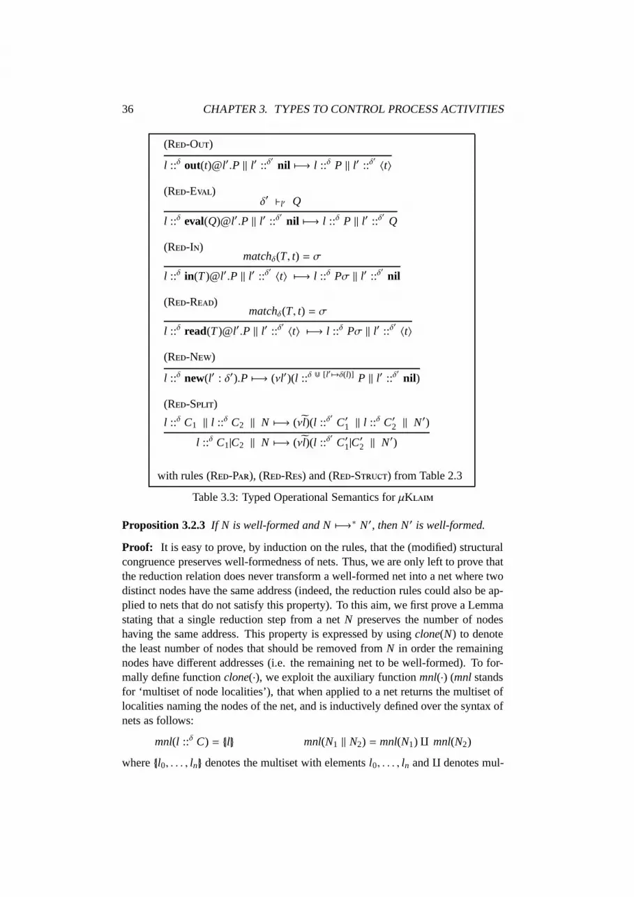
36 CHAPTER 3. TYPES TO CONTROL PROCESS ACTIVITIES
(R-O)
l ::δ out(t)@l′.P ‖ l′ ::δ′
nil 7−→ l ::δ P ‖ l′ ::δ′
〈t〉
(R-E)δ′ `l′ Q
l ::δ eval(Q)@l′.P ‖ l′ ::δ′
nil 7−→ l ::δ P ‖ l′ ::δ′
Q
(R-I)matchδ(T, t) = σ
l ::δ in(T )@l′.P ‖ l′ ::δ′
〈t〉 7−→ l ::δ Pσ ‖ l′ ::δ′
nil
(R-R)matchδ(T, t) = σ
l ::δ read(T )@l′.P ‖ l′ ::δ′
〈t〉 7−→ l ::δ Pσ ‖ l′ ::δ′
〈t〉
(R-N)
l ::δ new(l′ : δ′).P 7−→ (νl′)(l ::δ d [l′ 7→δ(l)] P ‖ l′ ::δ′
nil)
(R-S)
l ::δ C1 ‖ l ::δ C2 ‖ N 7−→ (νl)(l ::δ′
C′1 ‖ l ::δ C′2 ‖ N′)
l ::δ C1|C2 ‖ N 7−→ (νl)(l ::δ′
C′1|C′2 ‖ N′)
with rules (R-P), (R-R) and (R-S) from Table 2.3
Table 3.3: Typed Operational Semantics for µK
Proposition 3.2.3 If N is well-formed and N 7−→∗ N′, then N′ is well-formed.
Proof: It is easy to prove, by induction on the rules, that the (modified) structuralcongruence preserves well-formedness of nets. Thus, we are only left to prove thatthe reduction relation does never transform a well-formed net into a net where twodistinct nodes have the same address (indeed, the reduction rules could also be ap-plied to nets that do not satisfy this property). To this aim, we first prove a Lemmastating that a single reduction step from a net N preserves the number of nodeshaving the same address. This property is expressed by using clone(N) to denotethe least number of nodes that should be removed from N in order the remainingnodes have different addresses (i.e. the remaining net to be well-formed). To for-mally define function clone(·), we exploit the auxiliary function mnl(·) (mnl standsfor ‘multiset of node localities’), that when applied to a net returns the multiset oflocalities naming the nodes of the net, and is inductively defined over the syntax ofnets as follows:
mnl(l ::δ C) = |l| mnl(N1 ‖ N2) = mnl(N1) q mnl(N2)
where |l0, . . . , ln| denotes the multiset with elements l0, . . . , ln and q denotes mul-

3.2. A BASIC TYPE SYSTEM 37
tiset union. Now, for any µK net N, we can define clone(N) as the cardinalityof the multiset obtained by removing from mnl(N) one occurrence of each differentlocality occurring in it.
Lemma 3.2.4 If N 7−→ N′ then clone(N) = clone(N′).
Proof: We reason by induction on the length of the proof of the re-duction N 7−→ N′. The base case (i.e. one of the axioms (LTS-O),(LTS-E), (LTS-I), (LTS-R), (LTS-N) has been used) is ob-vious. In the inductive case, we reason by case analysis on the last ruleapplied. The cases of rules (LTS-P), (R-R) and (LTS-S) (itcan be easily seen that ≡ preserves clone(·)) easily follow by induction.Suppose now that the last applied rule is (R-S) and let N1 7−→ N2
be its premise. Then, due to the form of the nets involved in the rule,we have clone(N1) = clone(N) + 1 and clone(N2) = clone(N′) + 1.Since the proof of N1 7−→ N2 is shorter than that of N 7−→ N ′, we canapply induction and deduce that clone(N1) = clone(N2), from which itfollows that clone(N) = clone(N ′) that proves the thesis.
To conclude, note that a net N is well-formed if, and only if, clone(N) = 0. Hence,by using Lemma 3.2.4 and by a straightforward induction on the length of reductionsequences, the thesis easily follows.
3.2.3 Type Soundness
We first prove some standard results for type systems, i.e. weakening and substi-tutivity. Then, we show that (the modified) structural congruence preserves well-typedness; all these results will enable us to prove that the reduction relation pre-serves well-typedness. Then, we formalise the runtime errors we aim at eliminatingand prove that in well-typed nets runtime errors never occur. Finally, we can statethat a well-typed net never gives rise to runtime errors along any computation. Thisresult will be also generalised to deal with only partially well-typed nets.
Lemma 3.2.5 (Weakening) If Γ `l C then Γ′ `l C, for every Γ′ such that Γ Γ′.
Proof: Trivial.
Lemma 3.2.6 (Substitutivity)
1. If Γ `l C then, for any substitution σ, Γσ `l Cσ.
2. If Γ `l C and Γ `l Q, then Γ `l C[Q/X].
Proof:
1. The proof is by induction on length of the inference of the type judgement.The base cases (i.e., rules (T-N), (T-D) and (T-V)) are trivial.Let us examine the case in which the last rule used is (T-I); the casesfor (T-R), (T-O), (T-E), (T-N) and (T-P) are similar or

38 CHAPTER 3. TYPES TO CONTROL PROCESS ACTIVITIES
easier. By definition, C = in(T )@l′.P, Γ(l′) vΠi and upd(Γ,T ) `l P.
Without loss of generality, we can assume that dom(σ) ∩ bv(T ) = ∅ (oth-erwise, if this is not the case, we could rename the bound names); thuswe have that Cσ = in(Tσ)@(l′σ).(Pσ). Now, by induction, we have that(upd(Γ,T ))σ `l Pσ that easily implies upd(Γσ,Tσ) `l Pσ. Finally, it isclear that (Γσ)(l′σ) v
Πi; thus, we can apply rule (T-I) and conclude.
2. The proof proceeds by induction on length of the inference of the type judge-ment. The base cases, i.e. rules (T-N), (T-D) and (T-V), are triv-ial. If the last used rule is (T-R), the thesis easily follows by induction(recall that substitution application may require renaming of bound variablesto avoid capturing free names). If the last used rule is (T-P), the thesis fol-lows by induction using the fact that (C1|C2)σ = C1σ |C2σ. The cases whenthe last rule used is (T-I), (T-R), (T-O), (T-E) and (T-N)are similar; we examine only the first one. By definition, C = in(T )@l′.P,Γ(l′) v
Πi and upd(Γ,T ) `l P. By hypothesis, Γ `l Q; thus, by using
Lemma 3.2.5, we have that upd(Γ,T ) `l Q, since we can always assume thatbv(T ) ∩ fv(Q) = ∅. Then, by using the induction hypothesis, we get thatupd(Γ,T ) `l P[Q/X] and, by applying rule (T-I), we conclude.
Lemma 3.2.7 If N is well-typed and N ≡ N ′, then N′ is well-typed.
Proof: By mutual induction on the length of the inferences for N ≡ N ′ andN′ ≡ N. The base case covers the axioms in Table 2.2, except rule (S-C),and reflexivity of ≡. All the cases are trivial; just notice that the static typingis not affected if we coherently rename bound names within a net and that rule(S-R) relies on Lemma 3.2.6(2). The inductive step (for symmetry, transitivityand context closure) are easy.
Theorem 3.2.8 (Subject Reduction) If N is well-typed and N 7−→ N ′, then N′ iswell-typed.
Proof: By induction on the length of the inference of N 7−→ N ′.
Base Step: We reason by case analysis on the axioms (i.e. the first five rules) ofTable 3.3.
(LTS-O). Since by hypothesis N is well-typed, we have that δ `l out(t)@l′.P.Due to the form of the process involved, rule (T-O) has been the lastone applied to deduce the type judgement; hence we also have that δ `l P.Moreover, by applying (T-P) to δ′ `l′ C′ (that holds by hypothesis) andto δ′ `l′ 〈t〉 (axiom (T-D)), we get that δ′ `l′ C′ | 〈t〉. This suffices toconclude that N′ is well-typed.
(LTS-E). By reasoning like before, we can prove that δ′ `l′ P′ | Q. This easilyfollows by applying (T-P) to δ′ `l′ P′, that holds by hypothesis, and toδ′ `l′ Q, that is the premise of rule (R-E).

3.2. A BASIC TYPE SYSTEM 39
(LTS-I). Since it holds that δ′ `l′ nil, we are only left to prove that δ `l Pσ.Now, by hypothesis, we have that δ `l in(T )@l′.P, where rule (T-I) hasbeen the last one applied to infer the judgement; hence we also have thatupd(δ,T ) `l P. Now, let xi : πii∈I be the formal fields of T and lii∈I
be the corresponding names of t. By the premise of rule (LTS-I) and bythe definition of matchδ from Table 3.2, we have that matchδ(T, t) = σ,where σ = [li/xi]i∈I , and δ(li) vΠ πi for every i ∈ I. This means that [li 7→
πi]i∈I δ and upd(δ,T ) = δ d [xi 7→ πi]i∈I ; thus, (upd(δ,T ))σ = δ. ByLemma 3.2.6(1), we can conclude.
(LTS-R). Similar to the previous case.
(LTS-N). By hypothesis we have that δ `l new(l′ : δ′).P, where rule (T-N)has been the last one applied to infer the judgement. Hence we also havethat δ d [l′ 7→ δ(l)] `l P. The thesis follows by using Lemma 3.2.6(1) withsubstitution σ = [l′/l′].
Inductive Step: We reason by case analysis on the last applied operational rule ofTable 3.3.
(R-S). By hypothesis, we have that δ `l C1|C2. Due to the form of the pro-cess involved in the judgement, rule (T-P) has been the last one appliedto deduce the judgement; hence we also have that δ `l C1 and δ `l C2. Thus,we have that the net l ::δ C1 ‖ l ::δ C2 ‖ N is well-typed. By induction,we get that (νl)(l ::δ
′
C′1 ‖ l ::δ C′2 ‖ N′) is well-typed. It is easy to provethat δ(u) ⊆ δ′(u) for each u ∈ L; thus, the thesis directly follows by usingLemma 3.2.5.
(R-P). By hypothesis, N1 ‖ N2 is well-typed, hence N1 and N2 are well-typedtoo. Now, by induction, N ′1 is well-typed and hence N ′1 ‖ N2 is well-typed.
(R-R). By definition, (νl)N is well-typed if and only if N is well-typed; thissuffices to conclude by a straightforward induction.
(R-S). From the hypothesis, N is well-typed and N ≡ N1; by Lemma3.2.7, it follows that N1 is well-typed too. Now, by induction, we get thatN2 is well-typed. From this fact and from the hypothesis N2 ≡ N′, again byLemma 3.2.7, it follows that N ′ is well-typed.
Now, we introduce the notion of run-time error and state type safety, i.e. thatwell-typed nets do not give rise to run-time errors. Run-time errors are defined bythe rules in Table 3.4 in terms of predicate N that holds true when, within thenet N, a process P located at a node with address l attempts to perform an actionthat is not allowed by the access policy of the node. The rules are straightforward.
Notation 3.2.9 Here and in what follows, given an action a different from new, weuse arg(a) to denote its argument, tgt(a) its target location and cap(a) the capability

40 CHAPTER 3. TYPES TO CONTROL PROCESS ACTIVITIES
(EA)δ(tgt(a)) 6v
Πcap(a)
l ::δ a.P(EP)
N
N ‖ N′
(ER)N
(νl)N (ES)
N ≡ N′ N′
N
Table 3.4: Run-Time Error
corresponding to a. For example, if a is out(t)@l, then we have arg(a) = t, tgt(a) =l and cap(a) = o.
Theorem 3.2.10 (Type Safety) If N is well-typed then N does not hold.
Proof: We proceed by contradiction and prove, by induction on the length of theinference of N , that, if N , then N is not well-typed.
Base Step: In this case, the error is generated by using axiom (EA). Thismeans that N is a node of the form l ::δ a.P and δ(tgt(a)) 6v
Πcap(a).
Therefore, node l ::δ a.P, and hence N, is not well-typed otherwise rules(T-O), (T-E), (T-I), (T-R) or (T-N) would have failed.
Inductive Step: By case analysis on the last error rule used.
(EP). From the premise N of the rule and by induction, we have that N isnot well-typed. Hence, by definition, N ‖ N ′ is not well-typed too.
(ER). Similar.
(ES). From the premise N ′ of the rule and by induction, we have that N ′
is not well-typed. Then the thesis follows from the premise N ≡ N ′, by usingLemma 3.2.7.
Therefore, well-typed nets cannot immediately give rise to run-time errors. Now,by combining together the results shown so far, we get that well-typed nets nevergenerate run-time errors along sequences of reductions.
Corollary 3.2.11 (Global Type Soundness) If N is well-typed and N 7−→∗ N′,then N′ does not hold.
Proof: The proof proceeds by induction on the length of N 7−→∗ N′. The basestep is Theorem 3.2.10, while the inductive step follows from Theorems 3.2.8and 3.2.10.
Type soundness is one of the main goal of any type system. However, in ourframework it is formulated in terms of a property requiring the typing of whole nets.While this could be acceptable for LANs, where the number of hosts is usuallyrelatively small, it is unreasonable for WANs, where in general hosts are under the

3.3. DYNAMIC MANAGEMENT OF CAPABILITIES 41
control of different authorities. When dealing with larger nets, it is certainly morerealistic to reason in terms of parts of the whole net. Hence, we put forward amore local formulation of our properties and results. To this aim, we define therestriction of a net N to a set of localities S , written NS , as the subnet obtainedfrom N by deleting all nodes whose addresses are not in S . The wanted local typesoundness result can be formulated as follows.
Theorem 3.2.12 (Local Type Soundness) Let N be a net and S ⊆ fv(N). If NS iswell-typed and N 7−→∗ N′, then N′S does not hold.
Notice that in the previous statement, no assumption on the whole net N is made.The proof is similar to the proof of Corollary 3.2.11; in fact, local type soundnessis enforced by the dynamic checking performed when processes migrate, whichprevents ill-typed processes to get into NS .
3.3 Dynamic Management of Capabilities
The basic type system presented in the previous section suffers from the fact thatpolicies are fixed and can never change during computations. Indeed, mechanismssupporting modifications at run-time of access control polices and process capabil-ities turn out to be essential for dealing with pervasive network applications, like,e.g., those for e-commerce.
In this section, we discuss how our theory can be extended to take into accountvery flexible and sophisticated mechanisms to dynamically handle capabilities. Forthe sake of presentation, we will first introduce only the possibility for a policy tobe enlarged with new capabilities; then, we will argue on how implementing furtherdesirable features, like capability consumption, expiration and revocation.
Types and Grantings
As we have already said, actions new can only be performed locally. Hence, thecorresponding capability cannot be passed through. Since in this section we focuson capability passing, we only consider capabilities i, r, o and e, and, for the sake ofsimplicity, we assume that actions new are enabled everywhere. Types are definedlike in Definition 3.1.1 over this restricted set of capabilities. However, now typescan also change during computations; recall that the pointwise union of functionsδ1 and δ2, written δ1dδ2, is the type δ such that δ(u) = δ1(u)∪δ2(u) for each u ∈ L.
We allow capabilities to be passed at runtime by following the discretionaryaccess control model, where each principal owning a capability can pass it through.Policy modifications could be carried on by using specific primitives, like in [53].However, for the sake of economy, we prefer to merge it in the communicationprimitives. This means that capabilities are associated to tuples when performingan action out and are retrieved when performing actions in/read. More precisely,

42 CHAPTER 3. TYPES TO CONTROL PROCESS ACTIVITIES
each name occurring in a tuple argument of actions out is now equipped with agranting.
Definition 3.3.1 (Capabilities and Types – revisited) The set of capabilities C isr, i, o, e. We let Π be the powerset of C and use π to range over Π.
Types, ranged over by δ, are functions mapping L into Π such that δ(l) , ∅only for finitely many ls.
Definition 3.3.2 (Grantings) Grantings, ranged over by µ, are finite partial func-tions mapping L to Π.
Thus, the formal syntax of tuples from Table 2.4 is now changed to be
t ::= u : µ∣∣∣ t1, t2
Intuitively, grantings are used in actions out to point out some capabilities to bepassed through together with the names in the tuple. The intended meaning is that,if l retrieves a tuple 〈. . . , l′ : [· · · , l 7→ π, · · · ], . . .〉, then l receives the capability[l′ 7→ π].
We could decide to let dynamically acquired capabilities be exploitable onlyby the process that performed the in/read. However, this choice would imply thatthe policy of the node is not changed. Hence, our approach consists in changingthe policy of the node where the action was fired and sharing the new capabilitiesbetween all co-located processes. Moreover, since the exact moment in which anacquisition of capabilities takes place is unknown (because of the non determinismunderlying the operational semantics), we let all processes already in execution atl exploit the new capabilities. This choice is driven by the sake of fairness; indeed,it seems us unfair to assign new capabilities only to newly spawned processes.Unluckily, this choice requires more runtime checks. Indeed, an action that is stat-ically illegal could become legal upon acquisition of the capability enabling it. Forthis reason, if a process intends to perform an action not allowed by the policy ofthe node hosting it, the static typing system cannot reject the process since the ca-pability necessary to perform the action could in principle be dynamically acquiredby the node. In such cases, the typing system simply marks the action (turning ainto a) to require its dynamic checking. So, we shall define the operational se-mantics for nets written in an ‘intermediate language’, where marked actions canbe used to prefix a process. Notationally, we will write P (C and N, resp.) toemphasise that process P (component C and net N, resp.) may contain markedactions.
Finally, we also have to check grantings within actions out. This is necessaryto avoid capability forging like in
l ::δ out(l′ : [l 7→ π])@l.in(!x : π)@l
where [l′ 7→ π] 6 δ. If the first action was legal, the second action would addnew capabilities to δ and l would have enlarged its policy autonomously. This is a

3.3. DYNAMIC MANAGEMENT OF CAPABILITIES 43
clear security breach that must be avoided. Such an action out should be executedonly if δ(l′) v
Ππ. However, if we perform this check statically, dynamically ac-
quired capabilities could not be passed anymore; this somehow collides with thediscretionary access control, where a dynamically received capability becomes afirst-class capability (that must be handled like statically assigned ones). Thus, wedefer the check on grantings at run-time too.
3.3.1 Language Semantics
In this section, we present the static and the dynamic semantics of our calculus.For the sake of presentation, we will first introduce a basic setting where capabil-ities can only be acquired; in Section 3.3.4 we shall enrich it to deal with furtherdesirable features.
Static Semantics
We start with the static part of the language semantics. Informally, for each nodeof a net, say l ::δ C, the typing system determines if the actions that C intends toperform when running at l are enabled by the access policy δ or not. For example,capability e can be used to control process mobility: a process in C can migrate tol′ only if [l′ 7→ e] is a subtype of δ.
However, because a node can dynamically acquire capabilities when C ac-cesses data, some actions that can be permissible at run-time could be statically ille-gal; such actions are marked to be dynamically checked. The marking mechanismnever applies to actions whose targets are names bound by in/read, because suchactions can be statically checked, thus alleviating the burden of dynamic checkingand improving system performance. In fact, according to the syntax, whenever aname x is bound by an action in/read, it is annotated with a set of capabilities πthat specifies the operations that the continuation process is allowed to perform byusing x as the target address. Moreover, π also specifies the ‘minimal’ set of capa-bilities that the executing node must own or acquire over the net locality that willreplace x at run-time. Hence, our type system has to reject node
l1 ::[l′ 7→r] read(!x : o)@l′.read(!y)@x
because r does not belong to the annotation of x: this is a clear programming errorand the type system can statically check it. On the other hand, the type systemshould accept node
l2 ::[l′ 7→r] read(!x : o)@l′.out(t)@l′
because action out(t)@l′ can be marked and checked at run-time. In fact, if x isdynamically replaced with l′, l2 will acquire capability o over l′ and the processrunning at l2 can proceed; otherwise, the process will be suspended. In our sys-tem, the dynamic acquisition of capabilities is exploited exactly for relaxing the

44 CHAPTER 3. TYPES TO CONTROL PROCESS ACTIVITIES
(T-) (T-)Γ `L
l nil . nil Γ `Ll 〈t〉 . 〈t〉
(T-)X ∈ L
Γ `Ll X . X
(T-)
Γ `L∪Xl P . P
Γ `Ll rec X.P . rec X.P
(T-)
Γ `Ll C1 . C1 Γ `L
l C2 . C2
Γ `Ll C1 | C2 . C1 | C2
(T-)
cap(a) ∈ o, e Γ `Ll P . P
Γ `Ll a.P . markL(Γ)a.P
(T-)
cap(a) ∈ i, r upd(Γ, arg(a)) `L∪bn(arg(a))l P . P
Γ `Ll a.P . markL(Γ)a.P
(T-)
δ Γ d [l′ 7→ Γ(l)] Γ d [l′ 7→ Γ(l)] `L∪l′ l P . P
Γ `l new(l′ : δ).P . new(l′ : δ).P
Table 3.5: Typing Rules for Dynamic Capabilities Management
static type checking and admitting nodes like l2 while requiring on (part of) thema dynamic checking.
Type judgements for processes take the form Γ `Ll C . C. Here, L is a finite set
of names and it is used to keep track of bound names that have been freed duringthe inference as the result of removing a binding operator, i.e. in/read/new/rec.The environment Γ collects together the capabilities contained in the policy of land the type annotations for the names that have been freed in C. Intuitively, thejudgement Γ `L
l C . C states that, when C is located at l, the unmarked actions inC are admissible w.r.t. Γ. Instead, the marked actions in C cannot be deemed legalat compile time but could become permissible at run-time, after dynamic acquisi-tion of the necessary capabilities (via execution of actions in/read performed at l).When L is empty, we shall simply write Γ `l C . C.
Type judgements are inferred by using the rules in Table 3.5. The functionmarkL(Γ)· for marking process actions is defined as follows
markL(Γ)a =
a if Γ(tgt(a)) v
Πcap(a)
a if Γ(tgt(a)) 6vΠcap(a) and tgt(a) < L
where 6vΠ
denotes the negation of vΠ. Condition tgt(a) < L distinguishes actions
using localities as target from those using freed names, marking the formers andrejecting the latters (as previously explained).
The rules in Table 3.5 should be quite explicative, we only remark a few points.Rule (T-) says that located tuples always successfully pass the static type

3.3. DYNAMIC MANAGEMENT OF CAPABILITIES 45
µ = [li 7→ πi]i=1,...,k ∀ i = 1, . . . , k . δ(l) vΠπi
[[ l : µ ]]δ
[[ t1 ]]δ [[ t2 ]]δ
[[ t1, t2 ]]δ
Table 3.6: Checking Grantings
checking, regardless their contents. This choice simplifies the technical devel-opment; however, in order to check grantings therein, we require that no tupleis present in the net at the outset (data must all be produced via actions out, thatare dynamically checked). Rules (T-) and (T-) deal with recursive defini-tions and only accept processes whose process variables are bound by a rec. Rule(T-) deals both with process composition and with component composition.Rule (T-) deals with out and eval; as we already explained in Section 3.1, thearguments of these actions are not statically checked. Rule (T-) deals with ac-tions in and read; the type annotations in the formal fields of the template are usedto enrich the current type environment in order to type the continuation process.Action new is dealt with differently from the other actions by rule (T-) andis always statically checked (i.e. it is never marked). Indeed, new is always per-formed locally and the corresponding capability cannot be dynamically acquired.
We end this section by formalising the notion of well-typed net.
Definition 3.3.3 A net is well-typed if, for each node l ::δ C, there exists a compo-nent C such that δ `l C . C.
Dynamic Semantics
The first ingredient we need for defining the operational semantics is a mechanismto control the capabilities passed through while executing an action out from nodel′. This check is defined as the predicate [[ · ]]δ, that can be inferred by using therules in Table 3.6. [[ · ]]δ is parameterised with respect to δ, the policy of the nodel′ where the action out takes place. Intuitively, whenever a tuple passes the capa-bilities πi over l to li (thus, the tuple is of the form 〈. . . , l : [· · · , li 7→ πi, · · · ], . . .〉),we need to verify that l′ owned such capabilities.
Another ingredient we need is a formal way to say that a template and a tupledo match. The pattern-matching function, matchδl , is defined by the rules in Ta-ble 3.7 and is parameterised with the locality l and the access control policy δ ofthe node where it is invoked. A successful matching returns a type, used to extendthe type of the node executing the matching with the capabilities granted by thetuple, and a substitution, used to assign names to variables in the process invokingthe matching. We use σ to range over substitutions (with finite domain) of namesfor names, ε to denote the ‘empty’ substitution and to denote substitutions com-position. As usual, substitution application may require alpha-conversion to avoidcapturing of free names.
Notice that the node where the read/in is executed must be authorised to accessall the names occurring in the tuple accessed; this is verified by examining all the

46 CHAPTER 3. TYPES TO CONTROL PROCESS ACTIVITIES
(M1)l ∈ dom(µ)
matchδl (l′, l′ : µ) = 〈[ ], ε〉(M2)
δ(l′) ∪ µ(l) vΠπ
matchδl (! x : π, l′ : µ) = 〈[l′ 7→ π], [l′/x]〉
(M3)matchδl (T1, t1) = 〈δ1, σ1〉 matchδl (T2, t2) = 〈δ2, σ2〉
matchδl ( (T1, T2) , (t1, t2) ) = 〈δ1 d δ2, σ1 σ2〉
Table 3.7: Matching Rules for Dynamic Capabilities Management
grantings in the tuple. Indeed, the pattern-matching fails whenever l, the nodewhere the tuple is accessed, is not named in all the grantings within the tuple. Thisis explicitly required in the premise of rule (M1) and implicitly required by thefact that the µ(l) in the premise of rule (M2) must be defined. This feature permitscontrolling ‘immediate access’ to tuples, i.e. constraining the nodes from wheretuples can be accessed (see Section 3.3.3). Moreover, rule (M2) ensures that ifa read/in executed at l looks for a locality where performing the actions enabledby π, then locality l′ can be selected only if the union of the capabilities over l′
owned by l and of the capabilities over l′ granted to l by the tuple enables π. Thecapabilities granted by the tuple are then used to enrich the capabilities of l over l′.
Function matchδl satisfies the following property, whose proof can be easilydone by induction on the number of fields of the first argument of the function.
Proposition 3.3.4 If matchδl (T, t) = 〈δ′, σ〉 with dom(σ) = xii∈I , then δ′ = [li 7→πi]i∈I where, for every i ∈ I, ! xi : πi is a field of T , li : µi is the corresponding fieldof t and σ(xi) = li.
As we already said, the operational semantics relates µK nets that maycontain marked actions. It is given by a reduction relation, 7−→, which is the leastrelation induced by the rules in Table 3.8. Let us comment on the rules in Ta-ble 3.8. Rule (R-O) says that, before adding a tuple to a TS, the grantingswithin the tuple must be checked according to the policy δ of the node where theprocess performing the out runs. Rule (R-E) says that a process is allowedto migrate only if it successfully passes a type checking against the access policyof the target node. During this preliminary check, some process actions could bemarked to be effectively checked when at run-time. Rules (R-I) and (R-R)say that the process performing the operation can proceed only if pattern-matchingsucceeds. In this case, the access policy of the receiving node is enriched with thetype returned by the matching mechanism and the substitution returned along withthe type is applied to the continuation of the process performing the operation (andin the type annotations therein). Rule (R-M) says that the in-lined securitymonitor stops execution whenever the capability for executing a is missing.
Notice that Proposition 3.2.3 still holds in this framework. To conclude thissection, we informally present a simple but significant example where our settingturns out to be expressive and elegant; this informal presentation will be refinedin Section 3.3.3. Let lU be the address of a node representing the server of a

3.3. DYNAMIC MANAGEMENT OF CAPABILITIES 47
(R-O)[[ t ]]δ
l ::δ out(t)@l′.P ‖ l′ ::δ′
C′ 7−→ l ::δ P ‖ l′ ::δ′
C′|〈t〉
(R-E)δ′ `l′ Q . Q
l ::δ eval(Q)@l′.P ‖ l′ ::δ′
C′ 7−→ l ::δ P ‖ l′ ::δ′
C′|Q
(R-I)matchδl (T, t) = 〈δ′′, σ〉
l ::δ in(T )@l′.P ‖ l′ ::δ′
〈t〉 7−→ l ::δdδ′′
Pσ ‖ l′ ::δ′
nil
(R-R)matchδl (T, t) = 〈δ′′, σ〉
l ::δ read(T )@l′.P ‖ l′ ::δ′
〈t〉 7−→ l ::δdδ′′
Pσ ‖ l′ ::δ′
〈t〉
(R-N) l ::δ new(l′ : δ′).P 7−→ (νl′)(l ::δd[l′ 7→δ(l)] P ‖ l′ ::δ′
nil)
(R-M)l′ = tgt(a) δ(l′) v
Πcap(a) l ::δ a.P ‖ l′ ::δ
′
C′ 7−→ N
l ::δ a.P ‖ l′ ::δ′
C′ 7−→ N
with rule (R-S) from Table 3.3and rules (R-P), (R-R) and (R-S) from Table 2.3
Table 3.8: Operational Semantics with Dynamic Capabilities Management
given department and let lP be the address of a node representing the publisherof some on-line publications. We want to implement a protocol through whichthe department chief subscribes a ‘licence’ enabling all the department membersto access the on-line publications. In terms of access control, this means that theprotocol must extend the policy δ of node lU with the capability of reading papersfrom lP. Hence, upon completion of the protocol, lU ’s policy should become δ d[lP 7→ r]. Then, all the department members can spawn code over lU and thusretrieve lP papers by simply using the process
eval( read(paperTitle, !x)@lP .out(paperTitle, x)@lM )@lU
Action read(paperTitle, !x)@lP looks for a paper whose title is paperTitle andwhose body is a text B; if such a paper is found, it is copied in lM’s tuple space,where lM is the address of the department member who required the paper. In amore realistic scenario, the capability ‘read’ over lP will not be delivered foreverto lU . To model this scenario, we will also take into account means of managingcapabilities loss, in Section 3.3.4.
3.3.2 Type Soundness
In this section, we first present a type soundness result that involves whole nets;then, we point out the modifications needed to get a local type soundness result

48 CHAPTER 3. TYPES TO CONTROL PROCESS ACTIVITIES
relative to a subnet of a larger net.We start introducing the notion of executable nets that, intuitively, are nets
already containing all necessary marks (as if they have already passed a static typechecking phase).
Definition 3.3.5 A net is executable if, for each node l ::δ C, it holds that δ `l C .Cwhere, for inferring the type judgement, in addition to the rules in Table 3.5, onecan also use the rules
(T--) (T--)cap(a) ∈ o, e Γ `L
l P . P
Γ `Ll a.P . a.P
cap(a) ∈ i, r upd(Γ, arg(a)) `L∪bn(arg(a))l P . P
Γ `Ll a.P . a.P
that allow a process to already contain marked actions. For the sake of readability,the judgement Γ `l C . C will be written as Γ `l C.
Notice that executable nets are well-typed. Our main results will be stated in termsof executable nets; indeed, due to the dynamic acquisition of capabilities, well-formed nets that are statically deemed well-typed can still give rise to run-timeerrors. However, by marking those actions that should be checked at run-time,well-typed (and well-formed) nets can be transformed into executable nets that,instead, cannot give rise to run-time errors (see Corollary 3.3.11).
We now adapt the results in Section 3.2.3 to the new scenario. We only presentthe most relevant differences.
Lemma 3.3.6 (Weakening) If Γ `Ll C then Γ d Γ′ `L
l C.
Lemma 3.3.7 (Substitutivity)
1. If Γ `Ll C then, for any substitution σ, Γσ `L′
l Cσ where L′ = L − dom(σ).
2. If Γ `L∪Xl C, X < L and Γ `L
l Q, then Γ `Ll C[Q/X].
Proof:
1. The proof is by induction on length of the inference of the type judge-ment. The base cases (i.e., rules (T-), (T-) and (T-)) are ob-vious. Let us examine the case in which the last rule used is (T-) (thecases for (T-), (T-), (T-), (T-) and (T--/) aresimilar or easier). By hypothesis, for some process Q and action a suchthat Γ(tgt(a)) v
Πcap(a) ⊂ i, r, we have that C = a.Q and Γ `L
l a.Q;
thus, upd(Γ, arg(a)) `L∪bn(arg(a))l Q. Without loss of generality, we can
assume that dom(σ) ∩ bn(arg(a)) = ∅ (otherwise, if this is not the case,we could rename the bound names); thus we have (a.Q)σ = aσ.Qσ.Now, by induction, we have that (upd(Γ, arg(a)))σ `L′′
l Qσ, where L′′ =(L ∪ bn(arg(a))) − dom(σ) = (L − dom(σ)) ∪ bn(arg(a)) = L′ ∪ bn(arg(a)).Now, upd(Γσ, arg(aσ)) `L′′
l Qσ (indeed, it is easy to prove that (Γ1dΓ2)σ =(Γ1σ) d (Γ2σ)) and, by applying rule (T-), we conclude that Γσ `L′
laσ .Qσ, i.e. Γσ `L′
l (a.C)σ.

3.3. DYNAMIC MANAGEMENT OF CAPABILITIES 49
2. The proof proceeds by induction on length of the inference of the type judge-ment. The base cases (i.e., rules (T-), (T-) and (T-)) are obvi-ous. If the last used rule is (T-), the thesis easily follows by induction(recall that substitution application may require renaming of bound variablesto avoid capturing free names). If the last used rule is (T-), the thesis fol-lows by induction using the fact that (C1|C2)σ = C1σ |C2σ. The cases whenthe last rule used is (T-), (T-), (T-) or (T--/)are similar; we examine only the first one. By hypothesis, for some pro-cess P and action a such that Γ(tgt(a)) v
Πcap(a) ⊂ i, r, we have that
C = a.P and Γ `L∪Xl a.P; thus, for the premises of rule (T-), we
have that upd(Γ, arg(a)) `L∪X∪bn(arg(a))l P. By hypothesis, Γ `L
l Q thus,by using Lemma 3.3.6, we have that upd(Γ, arg(a)) `L
l Q. Moreover, wecan always assume that bn(arg(a)) ∩ fn(Q) = ∅; hence, it also holds thatupd(Γ, arg(a)) `L∪bn(arg(a))
l Q. Then, by using the induction hypothesis, we
get that upd(Γ, arg(a)) `L∪bn(arg(a))l P[Q/X] and, by applying rule (T-),
we obtain Γ `Ll a.(P[Q/X]), that is Γ `l (a.P)[Q/X].
Now we prove that the property of a net of being executable is an invariant bothof the structural congruence and of the reduction relation.
Lemma 3.3.8 If N is executable and N ≡ N ′ then N′ is executable.
Theorem 3.3.9 (Subject Reduction) If N is executable and N 7−→ N ′, then N′ isexecutable.
Proof: The proof proceeds by induction on the length of the inference of N 7−→N′. We only present the most peculiar cases.
(R-E). Since by hypothesis N is executable, we have that δ `l eval(Q)@l′.P.Due to the form of the process involved, rule (T-) has been the last oneapplied to deduce the last type judgement; hence we also have that δ `l P.Moreover, by applying (T-) to δ′ `l′ C′ (that holds by hypothesis) and toδ′ `l′ Q . Q′ (that is the premise of rule (R-E)), we get that δ′ `l′ C′ |Q′. This suffices to conclude that N ′ is executable.
(R-I). Since it holds that δ′ `l′ nil, we are only left to prove that δ d δ′′ `l Pσ.Now, by hypothesis, we have that δ `l in(T )@l′.P, where rule (T-) hasbeen the last one applied to infer the judgement; hence we also have thatupd(δ,T ) `bn(T )
l P. By definition, if xi : πii∈I are the formal fields of T ,we have that upd(δ,T ) = δ d [xi 7→ πi]i∈I . Moreover, by the premise ofrule (R-I) and by Proposition 3.3.4, we have that matchδl (T, t) = 〈δ′′, σ〉,where δ′′ = [li 7→ πi]i∈I and σ = [li/xi]i∈I . Now, upd(δ,T ) = δ d [xi 7→ πi]i∈I
implies that upd(δ,T )σ = δ d [li 7→ πi]i∈I = δ d δ′′. Thus, by applying
Lemma 3.3.7.1 to upd(δ,T ) `bn(T )l P, we conclude that δ d δ′′ `l Pσ.

50 CHAPTER 3. TYPES TO CONTROL PROCESS ACTIVITIES
(R-M). By hypothesis, we have that δ `l a.P. Due to the form of the processinvolved in the judgement, rule (T--) has been the last one appliedto deduce the judgement; hence we also have that upd(δ, arg(a)) `l P. Bythe premise of (R-M), we have that, when the reduction takes place,δ(tgt(a)) v
Πcap(a). Hence, by applying (T-)/(T-), we can derive
δ `l a.P, that, together with the hypothesis δ′ `l′ C′, implies that l ::δ a.P ‖l′ ::δ
′
C′ is executable. The thesis now follows by induction.
To prove type safety we still use the notion of run-time errors defined in Ta-ble 3.4. The rules are formally unchanged. Notice that, since marked actionsare checked at run-time, they cannot give rise to run-time errors. At most, whentheir execution is not permissible, the process that is trying to execute them blockswaiting for the acquisition of the corresponding capabilities by a parallel processrunning at the same node.
Theorem 3.3.10 (Type Safety) If N is executable then N does not hold.
Proof: Similar to the proof of Theorem 3.2.10.
Therefore, we can combine together the results shown so far as in Section 3.2.3.
Corollary 3.3.11 (Global Type Soundness) If N is executable and N 7−→∗ N′,then N′ does not hold.
Theorem 3.3.12 (Local Type Soundness) Let N be a net. If NS is executable andN 7−→∗ N′, then N′S does not hold.
3.3.3 Example: Subscribing On-line Publications
In this section, we take up the simple example presented at the end of Section 3.3.1in order to show µK’s programming style and a way to exploit its type systemfor establishing access control policies.
Suppose that a user U wants to subscribe a ‘licence’ to enable accessing on-line publications of a given publisher P. To model this scenario we use three local-ities, lU , lP and lC , respectively associated to U, P and to the repository containingP’s on-line accessible publications (this slightly differs from the informal scenariosketched in Section 3.3.1 – we explain later the reason why node lC is needed).First of all, U sends a subscription request to P including its address (together withan ‘out’ capability) and credit card number; then, U waits for a tuple that will de-liver it the capability r needed to access P’s publications and proceeds with the restof its activity. The behaviour described so far is implemented by the process
AU , out(“S ubscr”, lU : [lP 7→ o],CrCrd)@lP.in(“Acc”, !x : r)@lU .R
where process R may contain operations like read(. . .)@lC .

3.3. DYNAMIC MANAGEMENT OF CAPABILITIES 51
Once P has received the subscription request and checked (by possibly usinga third party authority) the validity of the payment information, it gives U a ‘read’capability over lC . P’s behaviour is modelled by the following process.
AP , rec X. ( in(“S ubscr”, !x : o, !y)@lP.
check credit card y of x and require the payment .out(“Acc”, lC : [x 7→ r])@x | X )
Concretely, the capability r will be delivered to U for a limited period of time (forexample, annual subscriptions would obtain read capabilities valid for one year) orfor a limited number of accesses. In Section 3.3.4 we shall present some simpleways to implement these features in our setting.
For processes AU and AP to behave in the expected way, the underlying netarchitecture, namely distribution of processes and access control policies, must beappropriately configured. A suitable net is:
lU ::[lU 7→o,i,r,e, lP 7→o] AU ‖ lP ::[lP 7→o,i,r,e,lC 7→o,i,r] AP
‖ lC ::[ ] 〈paper1〉 | 〈paper2〉 | . . .
where we have intentionally used AU to emphasise the fact that the statictype checking might have marked some actions occurring in AU , e.g. actionsread(. . .)@lC in R. Upon completion of the protocol, the net will be
lU ::[lU 7→o,i,r,e,lP 7→o,lC 7→r] R ‖ lP ::[lP 7→o,i,r,e,lC 7→o,i,r,lU 7→o] AP
‖ lC ::[ ] 〈paper1〉 | 〈paper2〉 | . . .
To conclude this section, we want to remark four features of this example thatshed light on some peculiarities of our framework.
1. P’s papers cannot be safely put in lP’s TS because otherwise the integrityof P’s publications could be compromised by the execution in lU of the le-gal process out(not−a−P ’s−paper)@lP. Indeed, differently from Section 3.4(see later on), our types do not provide support for restricting the kind of tu-ples over which actions can operate thus enabling out(“S ubscr”, lU : [lP 7→
o],CrCrd)@lP and disabling out(not−a−P ’s−paper)@lP.
2. Knowledge of address lC is not enough for reading papers: the ‘read’ capa-bility is needed. Indeed, security in the µK framework does not rely onname knowledge but on access control policies.
3. Once the ‘read’ capability over lC has been acquired, all processes eventuallyspawned at lU can access P’s on-line publications. In other terms, U obtainsa sort of ‘site licence’ valid for all processes running at lU . This fact shouldnot be considered as a security breach: indeed, in order to enter in lU , amobile process could be required to exhibit some credential (like a password[107]), that however we do not model in our framework. Moreover, noticethat this way of handling privileges is different from [59], where, by using

52 CHAPTER 3. TYPES TO CONTROL PROCESS ACTIVITIES
the same protocol, U would have obtained a sort of ‘individual licence’ forprocess R. In the next section we will present variations of our frameworkthat permit delivering different capabilities to co-located processes.
4. The licence delivered by P to U can be used only at lU since the grantingassociated to lC only delivers to lU the capability r over lC . Moreover, nointruder can interfere with the protocol between the user and the publisherbecause the tuple 〈“Acc”, lC : [lU 7→ r]〉 located at lU can only be retrievedby processes running at lU (see rules (M1) and (M2) in Table 3.7). A similarargument holds for the tuple 〈“S ubscr”, . . .〉 inserted by AU at lP.
3.3.4 Variations on Capability Management
Up to now, capabilities are always acquired by the node hosting the process per-forming actions in/read, and not by the process itself. This may be adequate insome cases, e.g. when a department subscribes a ‘site licence’ (i.e. valid for all itsmembers), and unrealistic in others, e.g. when a mobile process has to buy a goodon behalf of its owner. Moreover, capabilities can only increase; this does not fitwell to control wastable resources where one usually wants to count the number oftimes a given resource is used or to deliver accesses for a limited period of time.
In the next two subsections, we will show that our framework can be smoothlytailored for taking into account these different scenarios. For each variant, we shallfirst describe the scenario we want to model from an operational point of view (thatshould be more intuitive and that enables the presentation of a concrete examplemotivating the variation). Then, we shall discuss how the typing theory can beaccommodated to keep the results of Section 3.3.2 valid.
Variations on Capabilities Acquisition
In this section, we show an adaption of our framework that allows processes toacquire capabilities for themselves. We start by presenting a scenario where all thedynamically acquired capabilities are assigned to processes; then, we shall com-bine together the possibility of assigning capabilities to processes and to nodes.
(I) Acquisition by Processes. We start modifying our framework in such a waythat capabilities, in particular those dynamically acquired, can be associated toprocesses. To this aim, we annotate located processes with a type that specifies thecapabilities they own. Thus, a process can also use its own private capabilities, inaddition to the capabilities of the executing node that are shared by all co-locatedprocesses. Now, a µK node is of the form l ::δ AC, where AC is an annotatedcomponent generated from the following auxiliary syntactic productions
AC ::= 〈t〉∣∣∣ P δ
∣∣∣ AC1|AC2
Notice that only process components can be annotated.

3.3. DYNAMIC MANAGEMENT OF CAPABILITIES 53
(R-O′)[[ t ]]δdδ1
l ::δ out(t)@l′.P δ1 ‖ l′ ::δ′
AC′ 7−→ l ::δ P δ1 ‖ l′ ::δ′
AC′|〈t〉
(R-E′)δ′[δ1] `l′ Q . Q
l ::δ eval(Q)@l′.P δ1 ‖ l′ ::δ′
AC′ 7−→ l ::δ P δ1 ‖ l′ ::δ′
AC′| Q δ1
(R-I′)
matchδdδ1l (T, t) = 〈δ′′, σ〉
l ::δ in(T )@l′.P δ1 ‖ l′ ::δ′
〈t〉 7−→ l ::δ Pσ δ1dδ′′ ‖ l′ ::δ′
nil
(R-R′)
matchδdδ1l (T, t) = 〈δ′′, σ〉
l ::δ read(T )@l′.P δ1 ‖ l′ ::δ′
〈t〉 7−→ l ::δ Pσ δ1dδ′′ ‖ l′ ::δ′
〈t〉
(R-N′)
l ::δ new(l′ : δ′).P δ1 7−→ (νl′)(l ::δ P δ1d[l′ 7→δ1(l)] ‖ l′ ::δ′
nil)
(R-M′)
l′ = tgt(a) δ1(l′) vΠcap(a) l ::δ a.P δ1 ‖ l′ ::δ
′
AC′ 7−→ N
l ::δ a.P δ1 ‖ l′ ::δ′
AC′ 7−→ N
(R-S′1)
l ::δ AC1 ‖ l ::δ AC2 ‖ N 7−→ l ::δ AC′1 ‖ l ::δ AC′2 ‖ N′
l ::δ AC1|AC2 ‖ N 7−→ l ::δ AC′1|AC′2 ‖ N′
(R-S′2)
l ::δ P δ1 ‖ l ::δ Q δ1 ‖ N 7−→ l ::δ P′ δ2 ‖ l ::δ Q δ1 ‖ N′
l ::δ P|Q δ1 ‖ N 7−→ l ::δ P′ δ2 | Q δ1 ‖ N
plus rules (R-P), (R-R) and (R-S) from Table 3.8.[[ · ]] is defined in Table 3.6 and matchl(·, ·) is defined in Table 3.7
Table 3.9: Acquisition by Processes: Operational Semantics
The structural congruence is modified by replacing rules (S-A) and(S-A) in Table 2.2 with rules
(A′)P =α P′
l ::δ P δ′ ≡ l ::δ P′ δ′
(S-A′)
l ::δ AC ≡ l ::δ AC | nil δ′

54 CHAPTER 3. TYPES TO CONTROL PROCESS ACTIVITIES
Instead, the operational semantics is changed for managing the acquisition of ca-pabilities that now increases process type annotations while leaves types of nodesunchanged. In the initial configuration, all processes could have assigned the sameempty type or could have assigned different and more informative type annotations,reflecting different capabilities for the processes. Table 3.9 presents the modifiedreduction rules that should be self-explicative. Notice that in (R-M′) only thetype associated to the process is used to check admissibility of action a; indeed, thetype of the node does never change (i.e. it is statically known) and has already beenused in the static typing phase.
Let us now briefly revise the subscription example. If in the initial configura-tion all processes have assigned the empty type, the evolution of the net accordingto the modified semantics leads to
lU ::[lU 7→o,i,r,e,lP 7→o] R [lC 7→r] ‖ lP ::[lP 7→o,i,r,e,lC 7→o,i,r] AP
‖ lC ::[ ] 〈paper1〉 | 〈paper2〉 | . . .
where now R is the only process having the capability to access the papers stored atlC . Moreover, notice that the capability o over lU delivered by AU to AP disappearsupon completion of the parallel component running at lP that handles AU’s request.Indeed, at the end of its task such a component becomes nil [lU 7→o] and hencecan be removed by using rule (S-A′) above.
(II) Acquisition by Nodes and Processes. In practice, a (mobile) process couldacquire some capabilities and, from time to time, decide whether it wants to keepthem for itself or to share them with other processes running at the same node. Anexample of the first scenario is a mobile process that buys a book and obviouslywants the book to be delivered to its owner. An example of the second scenario isa process that subscribes a ‘site licence’ to enable accessing some on-line publica-tions to be shared with all members of a given department.
A simple way to model both cases is to use different acquisition actions de-pending on whether the acquisition should be made on behalf of the node or ofthe process. Hence, we could leave the operational semantics of actions in/readunchanged (i.e. as given in Section 3.3.1) apart for the replacement of processeswith annotated processes, add actions inpr(T )@u and readpr(T )@u to the syn-tax, and model their operational semantics by using rules akin to (R-I′) and(R-R′) in Table 3.9. In such a way, actions in/read would increase the typeof the node where they are executed while actions inpr/readpr would increase theprivate type of the executing process. Therefore, in this variant of the calculus,processes are more powerful because, whenever capabilities are acquired, they candecide to share these capabilities with the other co-located processes or not.
Of course, to control the new actions, we also need to introduce the corre-sponding capabilities and to extend the capability ordering relation. Finally, no-tice that, since node types can dynamically change (like in the original seman-tics), in rule (R-M′) the hypothesis δ1(l′) v
Πcap(a) must be replaced by

3.3. DYNAMIC MANAGEMENT OF CAPABILITIES 55
δ1(l′) ∪ δ(l′) vΠcap(a). Indeed, a marked action can be enabled both by the ca-
pabilities accumulated by the process and by the capabilities offered by the hostingnode.
Type Soundness. We now sketch how the results of Section 3.3.2 can be adaptedto the variant we have just presented (notice that the setting of Section 3.3.4(I) isclearly an instance of the theory we develop here). The static typing needs smoothextensions: it should consider annotated processes and it should let rule (T-)deal with actions inpr/readpr too. The first task can be carried on by adding thefollowing rule
(T-)Γ d δ `L
l P . P
Γ `Ll P δ . P δ
A marked annotated component AC is an annotated component that may containannotated marked processes of the form P δ. Then, well-typedness and exe-cutableness are defined like before, but take into account annotated components.
Definition 3.3.13 A net is well-typed if, for each node l ::δ AC, there exists acomponent AC such that δ `l AC . AC. A net is executable if, for each nodel ::δ AC, it holds that δ `l AC . AC (abbreviated as δ `l AC).
Finally, run-time errors are defined accordingly, by letting rule (EA) become
(EA′)δ(tgt(a)) ∪ δ′(tgt(a)) 6v
Πcap(a)
l ::δ a.P δ′
Thus, soundness of the revised framework can be formulated and proved like inTheorem 3.3.12. Notice that, by taking the set S to be fn(N), we easily obtain alsothe global type soundness of Corollary 3.3.11.
Managing Loss of Capabilities
In this subsection, we deal with some scenarios where capabilities can be lost. Thethree settings we shall present mainly differ in the formal definition of capabilitiesand in the way in which capabilities are lost. The main common feature is thatstatic typing is weakened since there are a lot of ingredients that can dynamicallychange. As it could be expected, more flexibility requires more run-time checks.
Since in this subsection we need to express capabilities removal, we introducenotation δ = δ1, δ2 to state that, for each u ∈ L, we have δ(u) = δ1(u) ∪ δ2(u),δ1(u) = δ(u) − δ2(u) and δ2(u) = δ(u) − δ1(u). A similar notation is exploited alsofor grantings.

56 CHAPTER 3. TYPES TO CONTROL PROCESS ACTIVITIES
(R-O′′)
[[ t ]]δδ1 = δ′1
l ::δ out(t)@l′.P δ1 ‖ l′ ::δ′
AC′ 7−→ l ::δ P δ′1 ‖ l′ ::δ′
AC′|〈t〉
(R-E′′)
δ1 = δ′1, δ′′1 δ′ `l′ Q . Q
l ::δ eval(Q)@l′.P δ1 ‖ l′ ::δ′
AC′ 7−→ l ::δ P δ′1 ‖ l′ ::δ′
AC′| Q δ′′1
(R-I′′)
matchδdδ1l (T, t) = 〈δ′′, σ, t′〉
l ::δ in(T )@l′.P δ1 ‖ l′ ::δ′
〈t〉 7−→ l ::δ Pσ δ1dδ′′ ‖ l′ ::δ′
nil
(R-R′′)
matchδdδ1l (T, t) = 〈δ′′, σ, t′〉
l ::δ read(T )@l′.P δ1 ‖ l′ ::δ′
〈t〉 7−→ l ::δ Pσ δ1dδ′′ ‖ l′ ::δ′
〈t′〉
(R-M′′)
l′ = tgt(a) δ1 = δ′1, [l
′ 7→cap(a)] l ::δ a.P δ′1 ‖ l′ ::δ′
AC′ 7−→ N
l ::δ a.P δ1 ‖ l′ ::δ′
AC′ 7−→ N
plus rules (R-N′), (R-S′1) and (R-S′2) from Table 3.9and rules (R-P), (R-R) and (R-S) from Table 2.3
Table 3.10: Consumption of Capabilities: Operational Semantics
Consumption. If we interpret the ‘acquisition of capabilities’ as the ‘purchaseof services/goods’, it seems natural that a process will lose the acquired capabil-ity once it uses the service. For example, by paying the price of a book a userpurchases one copy of the book; if he wants another copy, he has to pay again. Toenable multiple acquisitions and consumptions of capabilities, we should be able tocount the number of capabilities that nodes/processes have over each resource (thisis somehow similar to ‘affine’ capability types of [38]). To this aim, we modify oursemantic framework by working with multisets of capabilities, instead of sets; inparticular, Π now denotes the set of the multisets built upon i, e, r, o. All the oper-ations over and relations between sets used up-to now (i.e., union, subset inclusion,...) must be considered as operations over and relations between multisets.
We start considering the case of dynamic acquisition and consumption of ca-pabilities only by processes (see Section 3.3.4(I)). This means that node types arestatically known and left unchanged by the operational semantics. The operationalrules are modified as reported in Table 3.10. The main change is that process

3.3. DYNAMIC MANAGEMENT OF CAPABILITIES 57
capabilities must be deleted whenever used; this happens in rules (R-O′′),(R-E′′) and (R-M′′). Notice that the checking of grantings now deletesthe process capabilities passed in the tuple and returns the capabilities left. Itsformal definition updates Table 3.6 as follows:
µ = [li 7→ πi]i=1,...,k
δ1 = δ′1, [l 7→
⋃ki=1(πi − δ(l))]
∀ i = 1, . . . , k . (δ(l) ∪ δ1(l)) vΠπi
[[ l : µ ]]δδ1 = δ′1
[[ t1 ]]δδ1 = δ2[[ t2 ]]δδ2 = δ3
[[ t1, t2 ]]δδ1 = δ3
Finally, also pattern matching needs to be modified; now, when it is invokedby l on T and t, it returns a triple 〈δ′′, σ, t′〉. The difference is in the tuple t′
obtained by removing from the grantings within t all the capabilities granted to l(i.e., the capabilities collected in δ′′). This is necessary otherwise repeated accessesto a tuple via actions read would lead to a form of ‘capability forging’. Indeed,each time a process at l reads t, the capabilities in δ′′ would be delivered to theprocess. Since the read can be repeated an unbounded number of times (until 〈t〉 isavailable), it would be possible to acquire several times the capabilities in δ′′. Thenew formulation of function match relies on the following modification of rule(M2)
δ(l′) ∪ µ(l) vΠπ µ = µ′, [l 7→ (π − δ(l′))]
matchδl (! x : π, l′ : µ) = 〈[l′ 7→ (π − δ(l′))], [l′/x], l′ : µ′〉
where only the capabilities delivered by the tuple that are not already owned bythe executing node are used to enrich the policy of the executing process (this isneeded to avoid delivering the process capabilities already in δ). As concerns (M1),it is modified to additionally return the tuple passed as second argument to functionmatchδl , while (M3) is modified to additionally return the tuple resulting from theconcatenation of the two tuples returned by its premises.
Taking up the example of Section 3.3.3, we can now program the acquisition(and the consumption) of a fixed number of capabilities r over the on-line reposi-tory. The user explicitly requires a number k of capabilities r and the publisher willcharge on U’s credit card the cost of k accesses to its publications. The processesimplementing these behaviours are
AU , out(“S ubscr”, lU : [lP 7→ o],CrCrd, k)@lP.
in(“Acc”, !x : k × r)@lU .R
AP , rec X. ( in(“S ubscr”, !x : o, !y, !z)@lP.
check credit card y of x and charge the cost for z accesses .out(“Acc”, lC : [x 7→ z × r])@x | X )
where × r stands for the multiset with occurrences of capability r.
Type Soundness. Differently from Section 3.3.4, process capabilities do notplay any role in the static typing (thus, rule (T-) is missing): indeed, since they

58 CHAPTER 3. TYPES TO CONTROL PROCESS ACTIVITIES
can also decrease, it is statically impossible to rely on them to determine whethera given action will be legal at run-time or not. As an example, consider the netl ::[ ] P|Q [l′ 7→o], where P , out(t)@l′ and Q , out(t′)@l′. In this case, exactlyone between P and Q will be able to perform action out while the other processwill be blocked, depending on the execution order. However, it is impossible tostatically tell which one will evolve and which one will get stuck (and hence both ofthem have to be marked). Moreover, the static semantics differs from that presentedbefore because it has to mark all the actions, except those directly enabled by theaccess policy of the node where the inference takes place (i.e. those actions a suchthat δ(tgt(a)) v
Πcap(a), where δ is the type of the node). This is necessary to
properly handle nodes like l ::[l′ 7→i] in(!u : o)@l′.out(·)@l′.out(·)@u, whereaction in should be the only unmarked one after static typing. Indeed, if we usethe static typing of Section 3.3.1, the second action out would not be marked; thiscould generate a run-time error because if u is replaced by l′ upon execution of thein, then the acquired capability o (that enables the execution of the second actionout) would be consumed to perform the first action out.
Well-typed and executable nets are formally defined like in Definition 3.3.13;recall that process types are never used to infer judgements, because rule (T-)is missing here. Run-time errors are defined like in Section 3.3.4(II), i.e. by exploit-ing rule (EA′). Thus, type soundness can be still stated and proved similarlyto Theorem 3.3.12.
A more general framework. Finally, let us now briefly consider the generalsetting where both processes and nodes can dynamically acquire and consume ca-pabilities (see Section 3.3.4(II)). This scenario is the most expensive because astatic typing phase cannot be exploited at all and all actions must be checked atrun-time. In fact, since also node types can dynamically change, it is impossibleto statically determine if a given action will have the necessary capabilities at run-time. Moreover, both the type associated to a process and the type of the nodewhere the process is running can provide the process with the capability necessaryto perform a given action. In this case, the capability can be removed from the typeof the node or from the type of the process, and a strategy must be implemented.The operational rules can be easily modified to control capabilities and remove theused ones, but, to save space, we do not show the modified rules.
Validity duration. Another possible way of modelling capability lost is by in-troducing duration, as we already mentioned in the example of Section 3.3.3. Eachcapability can be assigned a validity duration by indexing it with a natural number(or ∞) representing a period of time during which the capability is valid, i.e. canbe used: a capability is available until its validity has not been expired. Thus, types(and grantings) map L to Π′, where Π′ is the powerset of C × (Nat ∪ ∞) and itis ranged over by p. For example, [l 7→ i10, o5, e∞] expresses the fact that it isstill possible to perform over l actions in for 10 time units, actions out for 5 timeunits and actions eval for ever. A capability associated to ∞ is called ‘persistent’

3.3. DYNAMIC MANAGEMENT OF CAPABILITIES 59
since its validity never expires; notationally, we write them without any annotation(notice that all the capabilities considered so far were indeed persistent).
The operational semantics of the basic framework needs to be modified tomodel time passing and the effect of time passing on validity durations. To pointout the passing of τ time units, we label net reductions with τ. All the rules inTable 3.8 except (R-P) and (R-S) represent computational steps andare assumed to be instantaneous; thus, the reductions occurring therein are labelledwith ‘0’. The reductions contained in rules (R-P) and (R-S) are insteadlabelled with a generic label τ. Of course, this choice is far from being realistic butit allows us to incorporate durations in our framework with very small modifi-cations and can model all real situations. Because of the intrinsic asynchronousnature of our nets, we assume that time can pass differently in different parts ofthe net but, at each node, time passes uniformly for all the processes running there.This behaviour is implemented by adding to the rules in Table 3.8 the followingone
(R-T) l ::δ Cτ−→ l ::(δ)−τ (C)−τ
Function (·)−τ is defined inductively as
(C1|C2)−τ = (C1)−τ | (C2)−τ
(〈t〉)−τ = 〈t′〉 with t′ obtained from t by replacing each µ with (µ)−τ
[ ]−τ = [ ]
([l 7→ p])−τ = [l 7→ p′]where p′ is obtained from p by:• subtracting τ to all the durations, and• deleting the capabilities with a non-positive duration
(δ d δ′)−τ = (δ)−τ d (δ′)−τ
(µ d µ′)−τ = (µ)−τ d (µ′)−τ
and it is the identity function in all the other cases. Thus, it can be easily seen thatwhen τ1 time units pass in l1 and τ2 time units pass in l2, the net l1 ::δ1 C1 ‖ l2 ::δ2
C2 evolves as follows:
l1 ::δ1 C1 ‖ l2 ::δ2 C2τ1−→ l1 ::(δ1)−τ1 (C1)−τ1 ‖ l2 ::δ2 C2τ2−→ l1 ::(δ1)−τ1 (C1)−τ1 ‖ l2 ::(δ2)−τ2 (C2)−τ2
Type Soundness. We can statically control only the operations that are enabledby persistent capabilities; all the other operations have to be marked, since it is notpossible to exactly know when they will be performed. In particular, all the actionshaving a variable as target must be marked. Moreover, to avoid forging capabilitydurations, we also need to ensure that a process delivers a capability with durationτ only if the capability is persistent or has a duration at least τ in the type of thenode where the process runs.

60 CHAPTER 3. TYPES TO CONTROL PROCESS ACTIVITIES
These tasks can be achieved by defining an ordering on Π′, written vΠ′
, asfollows
τ ≥ τ′
cτ vΠ′ cτ′
p1 ⊆ p2
p2 vΠ′ p1
p1 vΠ′ p′1 p2 vΠ′ p′2
(p1 ∪ p2) vΠ′
(p′1 ∪ p′2)
Clearly [[ · ]]δ, matchδl (·, ·) and markL(Γ)· now exploit this ordering. In particular,this fact implies that, since cap(a) returns a capability that is not annotated, action ais marked whenever a corresponding persistent capability is missing in the currenttyping environment. On the other hand, rule (R-M) still invokes v
Π, that can
be straightforwardly extended to annotated capabilities by ignoring durations.Well-typedness and executableness are still defined like in Definitions 3.3.3
and 3.3.5. Type soundness is then formulated and proved like in Corollary 3.3.11and Theorem 3.3.12: it relies on the run-time errors defined in Table 3.4, that arestill defined in terms of 6v
Π(properly extended to ignore validity durations). The
only difference is that, in stating and proving subject reduction (Theorem 3.3.9),
we also need to consider time passing, i.e. reductions of the formτ−→ . We omit the
easy details.
Revocation. We shall now touch upon a new scenario where capabilities can berevoked, i.e. a node can delete capabilities of other nodes. To rule out obviousnasty attacks, we allow l to remove a type δ from l′ only if l has previously passeda supertype of δ to l′ (notice that this complies with standard trends in discretionaryaccess control models). In doing so, we have also to take into account the fact thatseveral nodes could have passed δ to l′.
We let S to be the set of the finite subsets of L and we let s, s′, . . . to rangeover S. We now annotate capabilities, ranged over by c, with the identity of thedeliverers, thus obtaining the set of annotated capabilities Π′, ranged over by p.Formally, Π′ contains the subsets of r, i, o, e × S such that, if (c1, s1) ∈ p and(c2, s2) ∈ p, for some s1 , s2, then c1 , c2. Statically assigned capabilities takethe form (c, ∅) and are abbreviated as c. We let the preorder v
Π′on annotated
capabilities to be defined by the following rules:
s2 ⊆ s1 ∨ s1 = ∅
(c, s1) vΠ′(c, s2)
p1 ⊆ p2
p2 vΠ′ p1
p1 vΠ′ p′1 p2 vΠ′ p′2
(p1 ∪ p2) vΠ′
(p′1 ∪ p′2)
Grantings are left unchanged, i.e. they are finite partial functions from L to Π,while types now use annotated capabilities. We use γ to range over these annotatedtypes that, formally, are functions mapping L to Π′ such that γ(l) , ∅ only forfinitely many ls. E.g., the type [l 7→ (i, l1) , (o, l2, l3) ] used as access controlpolicy of node l′ enables actions in/out from l′ over l, and records that the capabil-ity i has been delivered by l1 while the capability o has been delivered by both l2
and l3. The subtyping relation between annotated types, ′, is defined like but ofcourse relies on v
Π′instead of v
Π. If γ1 and γ2 are annotated types, the extension

3.3. DYNAMIC MANAGEMENT OF CAPABILITIES 61
(R-O′′′)[[ t ]]pol(γ)
l ::γ out(t)@l′.P ‖ l′ ::γ′
C′ 7−→ l ::γ P ‖ l′ ::γ′
C′|〈t〉l
(R-E′′′)pol(static(γ ′)) `l′ Q . Q
l ::γ eval(Q)@l′.P ‖ l′ ::γ′
C′ 7−→ l ::γ P ‖ l′ ::γ′
C′|Q
(R-I′′′)matchpol(γ)
l (T, t) = 〈δ, σ〉
l ::δ in(T )@l′.P ‖ l′ ::δ′
〈t〉l′′
7−→ l ::γdδl′′
Pσ ‖ l′ ::δ′
nil
(R-R′′′)matchpol(γ)
l (T, t) = 〈δ, σ〉
l ::δ read(T )@l′.P ‖ l′ ::δ′
〈t〉l′′
7−→ l ::γdδl′′
Pσ ‖ l′ ::δ′
〈t〉l′′
(R-R)γ ′ = γ ′′, δl
l ::γ revoke(δ)@l′.P ‖ l′ ::γ′
C′ 7−→ l ::γ P ‖ l′ ::γ′′
C′
plus rules (R-N), (R-S), (R-P), (R-R) and (R-S)from Table 3.8, with γ in place of δ everywhere.[[ · ]] is defined in Table 3.6 and matchl(·, ·) is defined in Table 3.7
Table 3.11: Revocation of Capabilities: Operational Semantics
γ1 d γ2 is the annotated type γ′ such that γ′(u) = γ1(u) + γ2(u) for each u ∈ L,where p1 + p2 is inductively defined as
∅ + p = p
(c, s) + p =
(c, s ] s′) ∪ p′ if (c, s′) ∈ p and p′ = p − (c, s′)(c, s) ∪ p if (c, ) < p
((c, s) ∪ p) + p′ = (c, s) + (p + p′)
We let s1 ] s2 be s1 ∪ s2 if both si , ∅, and ∅ otherwise. Underlying the definitionof ] there is the assumption that, if a capability has been statically assigned to agiven node (and hence one of the si is the empty set), then no other node will everbe allowed to revoke it; a similar motivation inspired us the definition of v
Π′.
To enable capability revocations, we add operation revoke(δ)@` to the syntaxof µK actions. The new operational semantics is given in Table 3.11. The mainmodification w.r.t. Section 3.3.1 is a way to ‘sign’ a tuple with the identity of theproducer, so that, when capabilities contained in the tuple are acquired, the identityof the granter is properly recorded to enable their possible future revocation. Thiscan be obtained by letting located tuples take the form
〈t〉l
where l is the producer of the tuple. Then, when a policy is updated by exploiting

62 CHAPTER 3. TYPES TO CONTROL PROCESS ACTIVITIES
capabilities passed by a node l′′ (see rules (R-I′′′) and (R-R′′′)), the re-ceived capabilities are annotated with l′′, as expressed by notation δl
′′. Formally,for any u ∈ L, we let δl
′′(u) = (c, l′′) : c ∈ δ(u). In the first four rules ofTable 3.11, we used function pol(γ) that yields a simple (i.e., not annotated) typeδ by deleting from γ all capability annotations, and static(γ), that is the annotatedtype obtained from γ by removing all the capabilities that have not been staticallyassigned. Finally, rule (R-R) deals with revocations: it verifies that therevocated capabilities, δ, are present in the type γ ′ of l′, and that l was one of thegrantors of δ in γ ′.
We now show two possible uses of revoke in the example of Section 3.3.3. Thefirst use consists in an alternative way of implementing the subscription for a fixedperiod of time d. Indeed, if we do not introduce validity durations as previouslyshown, we can let P to manage timing information: once U’s capability r hasexpired, P can revoke it. A simplified process AP implementing this behaviour is
AP , rec X. ( X | in(“S ubscr”, !x : o, !y, !d)@lP.
check c.c. y of x and require the payment for duration d.out(“Acc”, lC : [x 7→ r])@x.out(x,Today() + d)@l′P.B )
B , rec Y. in(x, !s)@l′P.out(“check”, x,Today(),Today()≤ s)@l′P .( in(“check”, x,Today(), false)@l′P.revoke([lC 7→ r])@x| in(“check”, x,Today(), true)@l′P.out(x, s)@l′P.Y )
where l′P is a reserved locality where P stores timing information (we have silentlyused basic values representing dates and booleans, together with some obvious op-erations over them). Intuitively, process AP handles timing expirations by record-ing in l′P the expiration date of U’s subscription (given by function Today() + d).Then, process B repeatedly verifies the validity of the subscription by checkingwhether the current date (given by function Today()) is antecedent to the expira-tion date of U’s subscription. When expired, the capability enabling the access toP’s papers is revoked.
Another possible use of revoke in our example consists in revoking the accesscapability to a misbehaved user, e.g. a user that sold the acquired capability r to athird part at a lower price (thus being a tricky contender of P). Notice, however,that evidence of U’s crime cannot be implemented in our calculus (also in real lifethere would be an external authority entitled to discover the crime and inform thepublisher).
Type Soundness. We now adapt the static typing of Section 3.3.1 to the newscenario. First, notice that we do not need a specific capability to enable revoke:the operation is enabled only if l has previously delivered δ to l′, and this is checkedat run-time, see rule (R-R). Hence, the static typing system is modifiedadding the following rule
(T-)Γ `L
l P . P
Γ `Ll revoke(δ)@l′.P . revoke(δ)@l′.P

3.3. DYNAMIC MANAGEMENT OF CAPABILITIES 63
Moreover, rule (T-) now relies on ′.Like for the previous variants, the typing can only rely on statically assigned
capabilities; indeed, annotated capabilities can be revoked in unpredictable ways.Again, this forces us to also mark all those actions whose target is a variable be-cause we cannot know if the action will be enabled by a revocable capability ornot. This is why in rule (R-E′′′) we have used function static(·), that is alsoexploited to define well-typedness and executableness, as follows.
Definition 3.3.14 A net is well-typed if, for each node l ::γ C, there exists a com-ponent C such that
pol(static(γ)) `l C . C
A net is executable if, for each node l ::γ C, it holds that
pol(static(γ)) `l C . C
The definition of run-time errors now relies on the following variation of rule(EA)
pol(γ)(tgt(a)) 6vΠcap(a)
l ::γ a.P
and soundness of the revised framework can be formulated and proved like in The-orem 3.3.12.
To conclude, notice that, here and in the other variants on capability loss, thesoundness theorems can be essentially proved like in Section 3.3.2. This is due tothe fact that, for the static typing, we only consider the capabilities always avail-able, i.e. those capabilities that cannot be consumed, that never expires and thatcannot be revoked. The marking mechanism, that does never give rise to run-timeerrors, is exploited whenever capabilities that can become unavailable are required.
3.3.5 Discussion on Capability Management
We now briefly discuss some language design issues related to the management ofcapabilities. Our type theory is largely independent from the underlying language.More specifically, it is possible to define a type theory similar to the one for µKwe have presented in this section, whenever we have a language with the followingfeatures: (i) a set of (possibly remote) process operations and a set of correspond-ing capabilities, (ii) an ordering relation over capabilities, and (iii) some linguisticprimitives for exchanging capabilities.
Notice that, however, several choices were possible when defining most of thefunctions used throughout this section; we shall only comment on some of them.
• When a tuple is produced, no check is made to control that the capabilitiesdelivered through the tuple do agree with the access control policy of thenode where the tuple is being inserted. Such ‘compatibility’ check is desir-able if the point of view is taken that a node is responsible for the capabilities

64 CHAPTER 3. TYPES TO CONTROL PROCESS ACTIVITIES
it provides; clearly, this would give rise to a different notion of well-typednets. The check could be implemented by appropriately modifying the checkon grantings of Table 3.6 so that also the access control policy of the targetnode is taken into account.
• In rule (M2) only the capabilities actually required by the process enrich thetype of the node performing an action in/read. An alternative could be toenrich the type with all the capabilities delivered to the receiving node bythe producer of the tuple.
• The definition of grantings used here is simpler than that of [80]. In loc.cit.,we can write [l 7→ π] to mean that we want to pass to l all the capabilitiescurrently owned, except for those in π. By taking π = ∅, it is thus possible topass all the capabilities owned at run-time (that are statically unknown andunpredictable). Moreover, another way to make our theory more powerful isto add a reserved keyword others that could be used to denote all the nodes ofa net; thus, the granting [others 7→ π] would specify that the capabilities inπ are granted to any node. Both these features can be easily accommodatedin the theory presented in this section, but they require more run-time checksand more complicated definitions. Their integration in the framework wehave presented is an easy task and it is left to the interested reader.
The theory presented in Section 3.3.4 is perhaps the simplest way to modelcapabilities revocation. We conclude by sketching more elaborated scenarios.
• According to rule (R-R), the process revoke(δ)@l′.P is stuck if onlya subtype of δ is present in γ ′. If we want to avoid this block, we can definethe type γ1 u γ2 to be the greatest common subtype (w.r.t. ′) of both γ1 andγ2, and redefine (R-R) to be
γ ′ = γ ′′, (γ ′ u δl)
l ::γ revoke(δ)@l′.P ‖ l′ ::γ′
C′ 7−→ l ::γ P ‖ l′ ::γ′′
C′
Thus, we can remove from γ ′ the greatest subtype of δ delivered by l.
• The proposed formulation rules out direct attacks aimed at revoking as manycapabilities as possible to reduce the functionality of a system. These attackscan be mounted by executing actions revoke(δ)@l′ by a process runningat l, where l did not delivered δ to l′. However, one can easily imagine ascenario in which l spawns such a malicious process over an l′′ that deliveredδ to l′. A simple way to avoid this is to define two typing systems: thefirst one is `l, the other one, denoted by || l , is defined as the first one butwithout rule (T-). We still use `l in the definitions of well-typed and ofexecutable nets, while we use || l in rule (R-E) (in this way we blockincoming agents containing actions revoke). This solution can however be
3.4. FINE-GRAINED CONTROLS ON PROCESS ACTIVITIES 65
over-restricting: a better (but more complex) solution is to define || l in sucha way that revoke(δ)@l′ is deemed legal only if it is syntactically precededby an action out delivering l′ some supertype of δ.
• The last scenario we consider is when l1 delivers δ to l2 and then l2 deliversδ to l. Should it be legal for l1 to perform an action revoke over l? In theframework of Section 3.3.4 it is not. However, we could model this sce-nario by annotating capabilities with subsets of S; each such subset shouldrepresent all the (unordered) paths leading to the acquisition of the capabil-ity. E.g., if c is annotated with the set l1, l2 , l′1, l
′2, l′3 in the annotated
type of l, then c has been delivered to l through l1 and l2 and, independently,through l′1, l′2 and l′3. Clearly, the semantics has to be modified to enable allthe lis and l′js to perform actions revoke over l.
3.4 Fine-grained Controls on Process Activities
We now present a second evolution of the basic type system of Section 3.2; as wealready said, it can be readily combined with the theory of Section 3.3 to yield avery powerful and flexible mean to control program executions. The type systemwe present in this section mainly implements two ideas leading to a fine-grainedcontrol:
1. the type system exploits the source of mobile processes for granting themdifferent privileges, and
2. process capabilities regulate operations over parts of a tuple space (i.e., themultiset of all those tuples contained in the tuple space that can be describedby a given pattern).
These desirable features can be found in real systems like, e.g., UNIX, where dif-ferent users can have different privileges and different files can be manipulated bydifferent allowed operations.
3.4.1 Fine-grained Types
We start by adapting capabilities and types of Definition 3.1.1 to the new sce-nario. We want to implement policies such that, for example, if l trusts l′, then l’saccess control policy could accept processes coming from l′ (that will be calledl′-processes) and let them accessing any tuple in l’s TS. If l′ is not totally trusted,then l’s access control policy could grant l′-processes the capabilities for execut-ing in/read only over tuples that do not contain classified data, for example tuplesstarting with a field containing the value “public”.
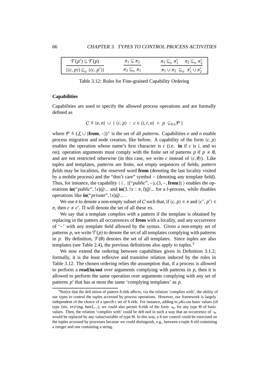
66 CHAPTER 3. TYPES TO CONTROL PROCESS ACTIVITIES
T (p′) ⊆ T (p)
〈c, p〉 vΠ〈c, p′〉
π1 ⊆ π2
π2 vΠ π1
π1 vΠ π′1 π2 vΠ π
′2
π1 ∪ π2 vΠ π′1 ∪ π
′2
Table 3.12: Rules for Fine-grained Capability Ordering
Capabilities
Capabilities are used to specify the allowed process operations and are formallydefined as
C , e, n ∪ 〈c, p〉 : c ∈ i, r, o ∧ p ⊆finP
where P , (L ∪ from,−)+ is the set of all patterns. Capabilities e and n enableprocess migration and node creation, like before. A capability of the form 〈c, p〉enables the operation whose name’s first character is c (i.e. in if c is i, and soon); operation arguments must comply with the finite set of patterns p if p , ∅,and are not restricted otherwise (in this case, we write c instead of 〈c, ∅〉). Liketuples and templates, patterns are finite, not empty sequences of fields; patternfields may be localities, the reserved word from (denoting the last locality visitedby a mobile process) and the “don’t care” symbol − (denoting any template field).Thus, for instance, the capability 〈 i , (“public”,−), (3,−, from) 〉 enables the op-erations in(“public”, !x)@... and in(3, !x : π, l)@... for a l-process, while disablesoperations like in(“private”, !x)@... .
We use π to denote a non-empty subset of C such that, if 〈c, p〉 ∈ π and 〈c′, p′〉 ∈π, then c , c′. Π will denote the set of all these πs.
We say that a template complies with a pattern if the template is obtained byreplacing in the pattern all occurrences of from with a locality, and any occurrenceof ‘−’ with any template field allowed by the syntax. Given a non-empty set ofpatterns p, we write T (p) to denote the set of all templates complying with patternsin p. By definition, T (∅) denotes the set of all templates. Since tuples are alsotemplates (see Table 2.4), the previous definitions also apply to tuples.3
We now extend the ordering between capabilities given in Definition 3.1.2;formally, it is the least reflexive and transitive relation induced by the rules inTable 3.12. The chosen ordering relies the assumption that, if a process is allowedto perform a read/in/out over arguments complying with patterns in p, then it isallowed to perform the same operation over arguments complying with any set ofpatterns p′ that has at most the same ‘complying templates’ as p.
3Notice that the definition of pattern fields affects, via the relation ‘complies with’, the ability ofour types to control the tuples accessed by process operations. However, our framework is largelyindependent of the choice of a specific set of fields. For instance, adding to µK basic values (oftype int, string, bool,...), we could also permit fields of the form −Θ, for any type Θ of basicvalues. Then, the relation ‘complies with’ could be defined in such a way that an occurrence of −Θwould be replaced by any value/variable of type Θ. In this way, a finer control could be exercised onthe tuples accessed by processes because we could distinguish, e.g., between a tuple field containinga integer and one containing a string.

3.4. FINE-GRAINED CONTROLS ON PROCESS ACTIVITIES 67
Types
Types, ranged over by ∆, are functions of the form
∆ : L ∪ any →fin ( ⊥ ∪ (L ∪ any, from →fin Π) )
where →fin means that the function maps only a finite subset of its domain tosignificant values (i.e. values different from ⊥ and ∅). With abuse of notation, weuse ⊥ to also denote the empty type, i.e. the function mapping any element of itsdomain to ⊥. Moreover, by letting λ to range over L ∪ any, from, we shall writeany ∆ different from ⊥ as a non-empty list [λi 7→ [λi j 7→ πi j ] j=1,...,ki]i=1,...,n; in thiscase, we shall denote the set λii=1,...,n as dom(∆).
Like before, types express the access control policies of nodes. Intuitively, ifthe type ∆ of a node with address l contains the element [l′ 7→ l′′ 7→ π], then l′-processes located at l are allowed to perform over l′′ only the operations enabledby π. The reserved word any is used to refer any node of the net. If it occurs inthe domain of ∆ then it collects the capabilities granted to processes coming fromany node of the net (i.e. [any 7→ l′′ 7→ π] grants all processes the capabilities πover l′′). If any is contained in the domain of ∆(l′), for some l′, then it is used fordenoting the operations that l′-processes located at l are allowed to perform overany node of the net (i.e. [l′ 7→ any 7→ π] grants l′-processes the capabilities πover all net nodes). The reserved word from stands for the last node visited bya process and is used to grant capabilities over this node whatever it is; thus, forinstance, [any 7→ from 7→ π] grants l′-process spawned at l the capabilities π overl′. The type ⊥ expresses total absence of capabilities.
We now revise the notion of subtyping; again, this notion is derived from thestandard preorder over functions, by also using the pointwise union of functions,denoted by d.
Definition 3.4.1 The subtyping relation, 6, is the least reflexive and transitive re-lation closed under the rule
∀ λ ∈ dom(∆1) : ∆1(λ) ∆2(λ) d ∆2(any)
∆1 6 ∆2
where extends the relation of Definition 3.1.3 to take into account associationsfor the reserved name any. Formally, it is the least reflexive and transitive relationclosed under the following rules:
m ≤ n ∀ i = 1, . . . ,m : π′i ∪ π′k vΠ πi
[λi 7→ πi]i=1,...,m [λ j 7→ π′j] j=1,...,n
λk = any
m ≤ n ∀ i = 1, . . . ,m : π′i vΠ πi
[λi 7→ πi]i=1,...,m [λ j 7→ π′j] j=1,...,n
∀ j.λ j , any

68 CHAPTER 3. TYPES TO CONTROL PROCESS ACTIVITIES
Notice that ⊥ 6 ∆ for any ∆, since dom(⊥) = ∅.We finally introduce the notion of well-formed types, that will be useful when
proving soundness of our system.
Definition 3.4.2 The type ∆ is l–well-formed whenever the following conditionshold:
1. If from ∈ dom(∆(λ)) then λ = any
2. For each λ ∈ dom(∆), it holds that ∆(λ) ∆(l)
Apart from technical reasons, this definition seems reasonable when considering∆ to be the type of locality l. Indeed, the first condition is not too restrictive,because the use of from is really necessary only when no knowledge of the lastnode visited by processes is available (i.e. when using any). The second conditionsays that l grants to λ-processes (for λ ∈ dom(∆)) no more capabilities than thosegranted to its local processes, i.e. those processes statically allocated at l. Thisseems reasonable because usually local code is more trusted than foreign codeand, hence, it is assigned more capabilities.
3.4.2 Static Semantics
For each node of a net, say l ::∆ C, the static type checker analyses the operationsthat the component C located at l intends to perform and determines whether theyare enabled by the access policy ∆ or not. A type context Γ is now a function ofthe form
L ∪ any →fin Π
The updating of a type context Γ with the type annotations specified within a tem-plate T is still denoted upd(Γ,T ) and is formally defined like in the previous sec-tions.
Type judgements for processes take the form Γ `∆l P and, like before, state that,within the context Γ, P can be safely executed once located at l, whose policy is ∆.Type judgements are inferred by using the rules in Table 3.13 that should be nowquite explicative. For operations out, in, read and eval, the inference requires thecapability associated to the operation to be enabled by the capabilities owned overthe target u or over all the net sites. Instead, for operation new, the capability nmust be owned by the site l executing the operation. In this case, it is assumed thatthe creating node owns over the created one all the capabilities it owns on itself.Moreover, the type ∆′, declared as the policy of the new node, must be well-formedfor l′ and less permissive than its creator’s type ∆. To this aim, we also need to addthe associations contained in Γ to ∆ when checking relation 6, since ∆′ is allowedto contain names that are in the domain of Γ but not in the domain of ∆: considerfor example the case of the process
in(!x : π)@l.new(l′ : [l′ 7→ x 7→ π′]). · · ·

3.4. FINE-GRAINED CONTROLS ON PROCESS ACTIVITIES 69
(T-N)
Γ `∆l nil
(T-D)
Γ `∆l 〈t〉
(T-V)
Γ `∆l X
(T-R)
Γ `∆l P
Γ `∆l rec X.P
(T-P)
Γ `∆l C1 Γ `∆l C2
Γ `∆l C1 | C2
(T-E)
Γ(u) ∪ Γ(any) vΠe Γ `∆l P
Γ `∆l eval(Q)@u.P
(T-O)
Γ(u) ∪ Γ(any) vΠ〈o, p〉 t ∈ T (p) Γ `∆l P
Γ `∆l out(t)@u.P
(T-I)
Γ(u) ∪ Γ(any) vΠ〈i, p〉 T ∈ T (p) upd(Γ, T ) `∆l P
Γ `∆l in(T )@u.P
(T-R)
Γ(u) ∪ Γ(any) vΠ〈r, p〉 T ∈ T (p) upd(Γ, T ) `∆l P
Γ `∆l read(T )@u.P
(T-N)
Γ(l) vΠn Γ d [l′ 7→ Γ(l)] `∆d [l7→l′ 7→∆(l)(l)]
l P
∆ is l′–well-formed ∆′ 6 ∆ d [l 7→ ([l′ 7→ ∆(l)(l)] d Γ])
Γ `∆l new(l′ : ∆′).P
Table 3.13: Inference Rules for the Fine-grained System
We conclude this section by defining well-typed nets w.r.t. the fine-grained typesystem.
Definition 3.4.3 A net N is well-typed if for each node l ::∆ C in N it holds that ∆is l–well-formed and ∆(l) `∆l C.
3.4.3 Dynamic Semantics and Type Soundness
Like in the previous sections, the operational semantics of Table 2.5 needs to bemodified by adding some runtime type checks. The structural congruence is readily

70 CHAPTER 3. TYPES TO CONTROL PROCESS ACTIVITIES
match∆(l)(l′, l′) = ε∆(l)(l′) ∪ ∆(l)(any) v
Ππ
match∆(l)(!u : π, l′) = [l′/u]
match∆(l)(T1, t1) = σ1 match∆(l)(T2, t2) = σ2
match∆(l)( T1, T2 , t1, t2 ) = σ1 σ2
Table 3.14: Matching Rules with Fine-grained Types
adapted from Section 3.2.2. With respect to Table 3.3, the main modifications affectthe pattern-matching predicate and the rules for actions eval and new. The reviseddefinition for pattern-matching readily extends the definition given in Table 3.2; forthe sake of clarity, its definition is given in Table 3.14. The main novelty is that,when trying to replace a formal field !u : π with a value l′, the capabilities ownedby l’s static code over any node can be added to the capabilities owned over l′ toobtain the needed capabilities in π.
The µK operational semantics with fine-grained types is the least relationinduced by the rules in Table 3.15. Let us comment on the key modifications. Rule(R-E) says that the migrating process Q must be checked against the unionof the capabilities that the access control policy ∆′ of the target node l′ assigns toprocesses coming from l and to processes coming from any node (in this last case,occurrences of from must be interpreted as l, as stated by the syntactic substitution∆′(any)[l/from] of from with l in function ∆′(any)).
To conclude, notice that Proposition 3.2.3 still holds in this framework.
Type Soundness.
We can now adapt the results of Section 3.2.3 to the setting of fine-grained types.The formulations of Lemmas 3.2.5 and 3.2.6 need to be slightly modified and theirproofs is carried-on like in Section 3.2.3; Lemma 3.2.7 is stated in the same wayand proved similarly.
Lemma 3.4.4 (Weakening) If Γ `∆l C then Γ′ `∆l C, for every Γ′ such that Γ Γ′.
Lemma 3.4.5 (Substitutivity)
1. If Γ `∆l C then, for any substitution σ, Γσ `∆l Cσ.
2. If Γ `∆l C and Γ `∆l Q, then Γ `∆l C[Q/X].
Theorem 3.4.6 (Subject Reduction) If N is well-typed and N 7−→ N ′, then N′ iswell-typed.
Proof: The proof is a smooth adaption of the corresponding one of Theorem 3.2.8;we only discuss the two most significant differences.

3.4. FINE-GRAINED CONTROLS ON PROCESS ACTIVITIES 71
(R-O)
l ::∆ out(t)@l′.P ‖ l′ ::∆′
nil 7−→ l ::∆ P ‖ l′ ::∆′
〈t〉
(R-E)
∆′(l) d (∆′(any)[l/from]) `∆′
l′ Q
l ::∆ eval(Q)@l′.P ‖ l′ ::∆′
nil 7−→ l ::∆ P ‖ l′ ::∆′
Q
(R-I)match∆(l)(T, t) = σ
l ::∆ in(T )@l′.P ‖ l′ ::∆′
〈t〉 7−→ l ::∆ Pσ ‖ l′ ::∆′
nil
(R-R)match∆(l)(T, t) = σ
l ::∆ read(T )@l′.P ‖ l′ ::∆′
〈t〉 7−→ l ::∆ Pσ ‖ l′ ::∆′
〈t〉
(R-N)
l ::∆ new(l′ : ∆′).P 7−→ (νl′)(l ::∆ d [l7→l′ 7→∆(l)(l)] P ‖ l′ ::∆′
nil)
(R-S)
l ::∆ C1 ‖ l ::∆ C2 ‖ N 7−→ (νl)(l ::∆′
C′1 ‖ l ::∆ C′2 ‖ N′)
l ::∆ C1|C2 ‖ N 7−→ (νl)(l ::∆′
C′1|C′2 ‖ N′)
with rules (R-P), (R-R) and (R-S) from Table 2.3
Table 3.15: Operational Semantics with Fine-grained Types
(R-E). Well-typedness of node l ::∆ P is inferred like in the previous case.We are only left to prove that ∆′(l′) `l′ Q since, by hypothesis, ∆′(l′) `l′ P′.By the premise of rule (R-E), we have that ∆′(l) d (∆′(any)[l/from]) `l′Q. If we prove that
∆′(l) d (∆′(any)[l/from]) ∆′(l′)
then we can conclude by using Lemma 3.4.4. Indeed, it suffices to provethat both ∆′(l) and ∆′(any)[l/from] are subtypes of ∆′(l′), since trivially thepointwise extension of partial functions respects this property. By l′–well-formedness of type ∆′, we have that:
• ∆′(l) ∆′(l′) (by condition 2. of Definition 3.4.2)
• let λ ∈ dom(∆′(any)[l/from]); then
– if λ , l then (∆′(any)[l/from])(λ) = ∆′(any)(λ) and, since

72 CHAPTER 3. TYPES TO CONTROL PROCESS ACTIVITIES
∆′(any) ∆′(l′) (again, by Definition 3.4.2(2)), it holds that∆′(l′)(λ) v
Π(∆′(any)[l/from])(λ)
– otherwise, it is easy to check that (∆′(any)[l/from])(l) is∆′(any)(l) ∪ ∆′(any)(from). By Definition 3.4.2(2), we have that∆′(l′)(l) v
Π∆′(any)(l). By Definition 3.4.2(1), we also know
that from < dom(∆′(l′)); hence, because ∆′(any) ∆′(l′) and byDefinition 3.4.1, it must be that ∆′(l′)(any) v
Π∆′(any)(l).
These facts amount to say that ∆′(any)[l/from] ∆′(l′).
(R-N). First of all, we have to prove that the types occurring in the resultingnet are still well-formed. Type ∆d[l 7→ l′ 7→ (∆(l)(l)−n)] is l–well-formed,since it is obtained from the l–well-formed type ∆ by adding capabilities tol-processes; type ∆′ is verified to be l′–well-formed by the static checker.Then, the fact that l ::∆ d [l7→l′ 7→∆(l)(l)] P is well-typed is proved similarly tothe case for (R-N) in Theorem 3.2.8; we leave the details to the reader.
The notion of run-time errors is adapted from Table 3.4 by upgrading rule(EA) as follows
∆(l)(tgt(a)) ∪ ∆(l)(any) 6vΠcap(a)
l ::∆ a.P
Theorem 3.4.7 (Type Safety) If N is well-typed then N does not hold.
Proof: Like in Theorem 3.2.10, we proceed by contradiction. The only relevantdifference is for the base case, where we have to reason on two sub-cases:
• a.P was part of a l′-process migrated to l. In this case, it cannot be ∆(l′) d(∆(any)[l
′/from]) `∆l a.P, otherwise, by Lemma 3.4.4, ∆(l) `∆l a.P and in
particular ∆(l)(tgt(a))∪∆(l)(any) vΠcap(a). But then, the premise of rule
(R-E) in Table 3.15 would not be satisfied and hence the migration ofthe l′-process containing a.P would have been blocked. This contradicts theassumption on the origin of process a.P.
• a.P was located at l at the outset. In this case, it must be that ∆(l)(tgt(a)) ∪∆(l)(any) 6v
Πcap(a), thus falsifying the premise of the static inference rule
for action a. This contradicts the well-typedness hypothesis.
Corollary 3.4.8 (Global Type Soundness) If N is well-typed and N 7−→∗ N′, thenN does not hold.
Theorem 3.4.9 (Local Type Soundness) Let N be a net. If NS is well-typed andN 7−→∗ N′, then N′S does not hold.

3.4. FINE-GRAINED CONTROLS ON PROCESS ACTIVITIES 73
3.4.4 Example: A Bank Account Management System
In this section, we use our approach to model the simplified behaviour of a bank ac-count management system. For ensuring compliance with the access control policyof the bank some aspects of our setting, such as the possibility of granting differentprivileges to processes coming from different source nodes and the dynamic typechecking of mobile processes when they migrate, have proved to be crucial.
We suppose that a bank is located at a node with address lB and can receiveand manage requests coming from many users located at nodes with addresseslU , lU′ , . . .. The bank must provide the users with typical account managing op-erations: opening/closing accounts, putting/getting money in/from accounts, andmaking statements of accounts. For simplicity, we shall omit some details andtechnical operations that in reality take place, like, e.g., charging taxes and dealingwith improper operations (like the attempt of getting more money than that reallyavailable).
For permitting the bank to check the operations that users intend to perform,we assume that users cannot perform remote operations over lB except for sendingprocesses. This can be achieved by using the type system presented in Section 3.3:the bank can pass its address, that should be fresh, only associated with the e capa-bility. Hence, if a user U wants to require an operation to the bank, it can only senda process to lB (thus virtually moving to the bank) which will interact locally withthe proper operation handler. The user process, once it has been accepted (i.e. afterits compliance with the bank access control policy has been checked), can requirethe operation by locally producing a tuple whose first field contains the name ofthe operation and whose second field contains the address of the user node (usedto identify the user that made the request). Depending on the operation, the tuplecould have other fields containing the amount of money involved in the operationand the account number receiving the money.
The node implementing the bank is illustrated in Table 3.16. First, the bankcreates a new node that will contain its clients accounts, stored as tuples of theform (userAddress, amount). This node acts just as a repository for tuples and willnot be used for spawning processes, thus it has assigned the empty type ⊥. Then,five different handler processes, one for each kind of operation, are concurrentlyspawned. Each handler continuously waits for a request. When such a requestarrives, the proper handler executes its task by remotely accessing the reservedlocality and then reports locally a confirmation of action completion. The clientprocess performing the request waits for such a confirmation and then brings it backto its original locality. This last operation is performed by means of a migrationthus providing the user node with the chance of controlling the operation.
Notice that, by taking advantage of the semantics of µK operations, thesimple handlers of Table 3.16 implement the mutual exclusion needed to ensurethe correctness of concurrent operations over shared data. Indeed, once a handlerH has withdrawn the tuple representing an account (i.e. once H has locked theaccount), the other handlers cannot perform other tasks on the same account until

74 CHAPTER 3. TYPES TO CONTROL PROCESS ACTIVITIES
lB ::∆B new(lS : ⊥).(OpenH(lS ) | PutH(lS ) | GetH(lS ) | ReadH(lS ) | CloseH(lS ))
where:
OpenH(u) , rec X.in(“open”, !x, !y)@l B.
(X | out(x, y)@u.out(“OKopen”, x, y)@l B)
PutH(u) , rec X.in(“put”, !x, !y, !w)@l B.
(X | in(w, !z)@u.out(w, z + y)@u.out(“OK put”, x, y,w)@l B)
GetH(u) , rec X.in(“get”, !x, !y)@l B.
(X | in(x, !z)@u.out(x, z − y)@u.out(“OKget”, x, y)@l B)
ReadH(u) , rec X.in(“read”, !x)@l B.
(X | read(x, !y)@u.out(“OKread”, x, y)@l B)
CloseH(u) , rec X.in(“close”, !x)@l B.
(X | in(x, !y)@u.out(“OKclose”, x, y)@l B)
∆B , [lB 7→ [lB 7→ i, o, r, n,any 7→ e ] ,
any 7→ [from 7→ e,lB 7→ 〈 o , (“open”, from,−),
(“put”, from,−,−),(“get”, from,−),(“read”, from),(“close”, from) 〉,
〈 i , (“OKopen”, from,−),(“OK put”, from,−,−),(“OKget”, from,−),(“OKread”, from,−),(“OKclose”, from,−) 〉
]]
Table 3.16: The node implementing the bank
H writes the updated tuple (i.e. H releases the lock).
The access control policy ∆B is so defined that ‘sensible’ operations over theaccounts of a user U (like getting some money and reading/closing the account)can only be requested by lU-processes, while operations like putting some moneycan be requested by processes coming from any node. Moreover, the only remoteoperation processes are allowed to perform is to came back to their source site.Therefore, a lU -process can request to the bank sensible operations only over U’saccounts and can deliver the confirmations only to lU . Typical processes acting onbehalf of a user U are illustrated in Table 3.17, where the parameter s denotes an

3.5. RELATED WORK 75
OpenR(s) , eval(out(“open”, l U, s)@lB.in(“OKopen”, l U, s)@lB.
eval(out(“OKopen”, s)@l U)@lU)@lB
PutR(s, lU′ ) , eval(out(“put”, l U , s, lU′ )@lB.in(“OK put”, l U, s, lU′ )@lB.
eval(out(“OK put”, s, l U′ )@lU )@lU)@lB
GetR(s) , eval(out(“get”, l U , s)@lB.in(“OKget”, l U , s)@lB.
eval(out(“OKget”, s)@l U)@lU )@lB
ReadR , eval(out(“read”, l U)@lB.in(“OKread”, l U, !x)@lB.
eval(out(“OKread”, x)@l U)@lU)@lB
CloseR , eval(out(“close”, l U)@lB.in(“OKclose”, l U , !x)@lB.
eval(out(“OKclose”, x)@l U)@lU)@lB
Table 3.17: Processes of a user U requesting bank operations
amount of money and the parameter lU′ denotes an account.The only possibility for a malicious node to illegally access U’s accounts is to
pass through lU , using a process like eval(eval(MaliciousReq)@lB)@lU . Hence,U has to protect itself from these attacks by granting an e capability over lB only toprocesses coming from totally trusted nodes: the access control policy of lU mustcontain the element [l 7→ lB 7→ e] only if U trusts the user located at l. However,U can trust l only if U trusts all l′ trusted by l (in fact, a node trusted by l cansend to l a process that is then allowed to spawn a process at U containing requestson U’s accounts). Notice that we do not aim at modelling here sophisticated trustmanagements; a wide literature on this topic is available and can be accommodatedin our setting.
Finally, notice that only the handler processes can access the node dynamicallycreated whose address is lS . Indeed, when such node is created, the operationalsemantics dynamically extends ∆B with [lB 7→ lS 7→ i, r, o] thus enabling all, andonly those, processes initially allocated at lB to perform in/read/out operationsover lS .
3.5 Related Work
There is a lot of work on type systems for security in calculi with process distri-bution and mobility. We conclude by surveying more strictly related work and bycontrasting it against the theory we have presented in this chapter.
A lot of type systems for GCs are strictly related to security; among the others,we mention those for controlling
• the types of the values exchanged in communications [39, 25, 90],
• Ambients mobility and ability to be opened [36, 37, 105, 69, 43],
• resource access via policies for mandatory and discretionary access control[26, 27],

76 CHAPTER 3. TYPES TO CONTROL PROCESS ACTIVITIES
• co-location of all processes that intend to access a given channel [139, 153],
• the effect of transmitted process abstractions over local channels [154, 87].
The research line closest to ours is that on the Dπ-calculus [90, 88, 129], wheretype systems control capabilities of mobile processes over located resources (i.e.communication channels). Differently from µK, node types describe permis-sions to use local channels (this is in sharp contrast with µK types that aim atcontrolling the remote operations that a network node can perform over the othernetwork nodes). For establishing well-typedness, the type system in [90] needsconsidering the whole net, while that in [88] only needs local information (becauseprocesses are dynamically checked whenever they migrate), and thus is similar toour approach. In [129], the global knowledge about the net is split into several parts(that are updated independently, but still in accordance with the global knowledge,via dynamic knowledge acquisition through communication) and, to reduce theamount of dynamic controls, a relation of trust among nodes is exploited (thus, noprocess coming from a trusted node is type checked).
[153] presents Dπλ, a process calculus that results from the integration of thecall-by-value λ-calculus and the π-calculus, together with primitives for processdistribution and remote process creation. Apart from the higher order and channel-based communication, the main difference with µK is that Dπλ localities areanonymous (i.e. not explicitly referrable by processes) and simply used to expressprocess distribution. Dπλ comes equipped with a type system that controls howprocesses use resources (i.e. channels) by guaranteeing that in well-typed systemsprocesses that intend to perform inputs at a given channel are co-located. In [154],a fine-grained type system for Dπλ is defined that permits controlling the effectof transmitted process abstractions (parameterised with respect to channel names)over local channels. Processes are assigned fine-grained types that, like interfaces,record the channels to which processes have access together with the correspondingcapabilities, and process abstractions are assigned dependent functional types thatabstract from channel names and types. This use of types is akin to µK’s one,though the differences between the underlying languages still remain.
Recently [87], the Dπ has been extended to allow high-order data to be trans-mitted. In the resulting formalism, called SafeDpi, parameterised code may be sentbetween sites using higher-order channels. A host location may protect it self byonly accepting code which conforms to a given type associated to the incomingport. A sophisticated static type system is then defined for these ports to restrictthe capabilities and access rights of any process launched by incoming code. De-pendent and existential types are used to add flexibility, allowing the behaviourof these launched processes to depend on the host’s instantiation of the incomingcode. However, similarly to [90, 154], the approach strongly relies on a global typ-ing environment to type the whole net. In our view, this is a too demanding requestin a global computing framework.
Finally, we want to mention some proposals for the Mobile Ambients calculusand its variants, albeit their network models and mobility mechanisms are very dif-

3.5. RELATED WORK 77
ferent from those of µK. As an example, we want to mention some differencesbetween the mobility control in Ambient and in µK deriving from their dif-ferent programming choices. Mobility in µK is, using Ambient terminology,objective (in that the moving process is spawned by an external process), whilemost of the work on Ambient–derived calculi uses subjective moves (explicitlyprogrammed in the moving entities). The mobility control defined in [105] for theSafe Ambient Calculus (similar to that presented in [38] for the Mobile Ambientcalculus) consists in identifying those ambients, called immobile, that cannot beopened and autonomously move, but can host local message exchanges and canreceive incoming ambients (that, however, cannot be opened therein). A somehowsimilar behaviour can be implemented in µK by setting the policy of a node lto be [l 7→ r, i, o, e, n]; however, this type cannot rule out remote communicationsusing l as the target node since l’s type cannot restrict actions remotely performed.[69] extends [105] by introducing ambient security levels: the types used there ruleout the movement through (and the opening of) ambients of lower security levels.We believe that this feature can be easily introduced in the µK setting.

78 CHAPTER 3. TYPES TO CONTROL PROCESS ACTIVITIES

Chapter 4
Types for Confining Data andProcesses
The major goal of language-based security is the design of languages that are flex-ible, expressive and safe. Unfortunately, these are often contrasting requirements.For example, mobile code deeply increases flexibility and thus expressiveness ofprogramming languages, but introduces new security problems related to unwantedaccesses to classified data. Standard security issues (like, e.g., secrecy and integrityof data and program code) are complicated by the presence of code mobility: theuse of cryptography, that is one of the most diffused techniques for ensuring secu-rity in distributed systems, must be strongly restricted in order to be safe. Indeed,malicious nodes can attack a mobile process and compromise its integrity throughcode modification or its secrecy through leakage of sensitive data. Similarly, mali-cious mobile processes might attempt to access or forge private data of the networknodes hosting them. Hence, we can hardly imagine to use mobile processes car-rying confidential data (e.g. private keys) with them, or host nodes with classifiedinformation accessible to all incoming processes (whatever their source node be).Hence, the use of security mechanisms that back up and supplement cryptographicmechanisms becomes a major issue when developing systems of distributed andmobile processes where the compliance with some security policies must be guar-anteed.
In this chapter, we define an approach that permits protecting the secrecy ofboth data residing on hosting nodes and of data carried by mobile processes, byrelying on program annotation. Our approach is inspired by Confined-λ [98] andrelies on annotating data with sets of node addresses, called regions, that specify thenetwork nodes that can interact with them. Also nodes may have annotations thatspecify which nodes can send data and spawn processes to them. Data annotationsenable programmers to control the set of nodes that can share specific data, andpermit shading them from other nodes. Node annotations, instead, enable nodeadministrators to control the set of data and processes each node can host; thus, thenode can refuse malicious processes and unwanted data.
79

80 CHAPTER 4. TYPES FOR CONFINING DATA AND PROCESSES
The language semantics is then designed to guarantee that computations pro-ceed while respecting the region constraints. For example, a process P can accessa datum d only if P’s execution does not export d outside its data region, say r,i.e. if P only writes d in network nodes included in r or, similarly, if P only carriesd while migrating to nodes included in r. Enforcing similar constraints requiresa form of code inspection that is performed, as much as possible, statically. Thisrelieves the runtime semantics of the burden to make expensive checks and, then,improves efficiency.
The approach we shall present here is largely independent of a specific model:indeed, in [61] we adapted our approach to other two paradigmatic calculi for GC,namely Dπ [90] and Mobile Ambients Calculus [41].
4.1 Controlling Data Movement via Types
We now set up a machinery based on typing that helps in protecting exchanged andlocal data in global computing applications. To this aim, we suggest annotatingdata with sets of network addresses, describing the sub-net where data can be used;these sets will be called regions and are formally defined as follows.
Definition 4.1.1 (Regions) Regions, r, are either finite subsets of names or thedistinct element >, used to refer to the whole net. The set of all regions is R; it ispartially ordered by the subset inclusion relation ⊆ and has > as top element.
The syntax of Table 2.4 is changed as follows:
N ::= . . .∣∣∣ l rd:: rp C
∣∣∣ . . .
t ::= [u]r
∣∣∣ . . .
The annotations allow programmers to fix the nodes that can share a given datum,and to avoid that the datum is accessed by untrusted processes (from untrustednodes). Also network nodes are annotated with regions that specify the nodes thatcan send data and those that can spawn processes to them. Thus, nodes are an-notated with two regions, say rd and rp. We should have rp ⊆ rd since acceptingprocesses is, in general, more dangerous than accepting data; however, no restric-tion on the model is imposed to deal with this issue. We shall assume that absenceof region annotations stands for >.
The language semantics guarantees that computations proceed according toregion constraints. This property, that we call safety, can be intuitively stated as “Anet N is safe if, for any datum d occurring in N associated to region r and for allpossible evolutions of N, it holds that d will only cross and reside at nodes whoseaddresses are in r”.
To better understand the properties we want to model and the impact of ourapproach on system security, we present a simple client/server example. Supposethat a client C requires a service to a server S . Once S has verified the credentials of

4.2. STATIC INFERENCE AND CHECKING 81
C (e.g. its identity or its credit card information), it sends back a secret password,that C can change. C could then access the service by using the last set password.This protocol can be modelled by assuming two network addresses, lC and lS ,hosting the processes PC and PS , respectively, defined as
PC , out(lC , [cc in f o]lC ,lS
)@lS .in(!y)@lC .< modi f y the password y and access the service >
PS , rec X.in(!x1, !x2)@lS .( X | < check the credit card in f o x2 > .
new(pwd).out([pwd]x1 ,lS
)@x1.
< handle password modi f ications and provide the service >)
We marked the information on C’s credit card with region lC , lS with the intentionthat only processes at the locations of C and S will be enabled to capture C’srequest. Thus, no attacks mounted from other nodes aimed at cancelling the requestcan take place. Similar considerations do hold for the restricted name pwd that Ssends back to C (it represents a secret password shared between processes at C’sand S ’s locations).
To make our theoretical framework properly working, we need to control theprocesses arriving at C’s and S ’s locations; this is why our typing discipline re-quires also nodes to be annotated with regions. Server S can then accept onlyprocesses coming from trusted nodes, but it should accept data coming from anyuser; this is necessary to model a setting where S accepts any service request, whileit supplies the service only to accredited users. Thus, lS ∈ rC
d and lC ∈ rSd (usually,
rSd = >), while rC
p = rSp = ∅.
It has to be said that we are implicitly assuming the ability of determining theorigin (the source node) of data and processes. By relying on it, we can then checkcompliance with region annotations.
4.2 Static Inference and Checking
The language presented in the previous section is a mean to program applicationswhere, during the computation, a datum can only appear in localities containedin its region annotation. The runtime semantics can enforce this requirement byperforming appropriate checks. These (runtime) checks are necessary because thepattern matching based communication does not permit making any static assump-tion on the actual structure of tuples hosted by a tuple space (see the discussionon this topic in the previous chapter). To make the semantics as efficient as possi-ble, a preliminary typing phase is introduced. The typing of µK nets aims atguaranteeing that:
1. a datum [l]r can be seen at (i.e. can cross) u if u ∈ r
2. a process retrieving a datum [l]r cannot exhibit l outside r.

82 CHAPTER 4. TYPES FOR CONFINING DATA AND PROCESSES
(T-E)
0 0
(T-N)N1 N′1 N2 N′2
N1 ‖ N2 N′1 ‖ N′2
(T-R)
N N′
(νl)N (νl)N′
(T-N)
rd, rp ∈ > ∪ 2L ∅ ` P l ∅ ` P′
l rd:: rp P l rd:: rp P′
Table 4.1: Static Typing for Confining Data and Processes (Nets)
The typing phase performs check 1. statically and annotates bound names occur-ring in templates with regions to enable efficient execution of check 2. at runtime.To better distinguish the annotations put by the programmers/administrators fromthose put by the type system, we shall write the latter ones as superscripts and theformer ones as subscripts. Hence, the syntax of templates from Table 2.4 becomes
T ::= u∣∣∣ [! x]r
∣∣∣ T1,T2
Intuitively, [! x]r states that the datum replacing x will cross at most the localitiesin r.
The typing procedure for µK nets is given in Table 4.1. Net typings arewritten N N′. The typing step includes a type checking phase, to verify that netsare written according to the region annotations therein, and a type inference phase,to annotate parameters occurring in templates. Intuitively, the inference phase takesa net N and returns a net N′ obtained from N by annotating all the parameters witha region containing the nodes that the received values will cross. E.g., in processin(!x)@l.out([x]r)@l′ the declaration !x of variable x must be associated to regionr that, in turn, must contain l′ (and l, of course). The type checker verifies that eachprocess located at a node l contains only data that can be seen by l (this is done bythe judgement l) and verifies that actions out and eval send data/code to nodeswhere the data/code can appear without violating the region annotations.
Judgement relies on an auxiliary procedure Γ ` P u Γ′ ` P′ defined in
Table 4.2, where the type environment Γ is a finite map from variables to regions.The procedure Γ ` P u Γ
′ ` P′ determines, for each parameter in P, a re-gion annotation describing the use of that parameter in the continuation process(i.e. where it will be sent); P′ is then obtained by decorating P with those annota-tions. Such regions are determined by the type inference by considering the localitywhere the process runs (the u decorating u) and by examining the localities wherethe variables can appear upon execution of actions out and/or eval.
Notice, however, that care is needed to avoid inconsistencies on names occur-ring in a process. As an example, consider the nodes (both of them are legal)
l :: in(!x)@l′.in(!y)@l′′.out([x]l,y)@l (?)
l :: in(!y)@l′.out([y]l,y)@l (??)

4.2. STATIC INFERENCE AND CHECKING 83
(T-N)
Γ ` nil u Γ ` nil
(T-P)Γ ` C1 u Γ
′ ` C′1 Γ′ ` C2 u Γ′′ ` C′2
Γ ` C1|C2 u Γ′′ ` C′1|C
′2
(T-D)u ∈ reg(t)
Γ ` 〈t〉 u Γ ` 〈t〉
(T-R)
Γ ` P u Γ′ ` P′
Γ ` rec X.P u Γ′ ` rec X.P′
(T-V)
Γ ` X u Γ ` X
(T-N)Γ ` P u Γ
′ ` P′
Γ ` new(l).P u Γ′ l ` new(l).P′
(T-I)Γ ] x : ux ∈ bn(T ) ` P u Γ
′ ] x : rxx ∈ bn(T ) ` P′
Γ ` in(T )@u′.P u Γ′bn(T ) ` in(T ′)@u′.P′
(∗)
(T-R)Γ ] x : ux ∈ bn(T ) ` P u Γ
′ ] x : rxx ∈ bn(T ) ` P′
Γ ` read(T )@u′.P u Γ′bn(T ) ` read(T ′)@u′.P′
(∗)
(T-O)u, u′ ⊆ reg(t) = r Γ ` P u Γ
′ ` P′
Γ ` out(t)@u′.P u Γ′ + x : rx ∈ fn(t) ` out(t)@u′.P′
(T-E)u ∈ reg(P1) Γ ` P1 u′ Γ
′ ` P′1 Γ′ ` P2 u Γ′′ ` P′2
Γ ` eval(P1)@u′.P2 u Γ′′ + x : u′x ∈ fn(P1) ` eval(P′1)@u′.P′2
(∗) is: T ′ obtained from T by replacing each !x with [! x]r′x ,
for r′x =
> if (rx − x) ∩ bn(T ) = ∅rx − x otherwise
Table 4.2: Static Typing for Confining Data and Processes (Components)
Blindly annotating these nodes would result in
l :: in([!x]l,y)@l′.in([!y]l)@l′′.out([x]l,y)@l
l :: in([!y]l,y)@l′.out([y]l,y)@l
Here, the occurrence of y in the regions of !x and !y respectively escaped its binder;thus, the y occurring in the annotations are not the same as the y bound in actionin. The solution we designed to accept (?) is to assign !x the region annotation >.This is reasonable since in([!x]l,y)@l′ means ‘retrieve a datum from l′ and share it

84 CHAPTER 4. TYPES FOR CONFINING DATA AND PROCESSES
with a generic locality of the net’ (indeed y can be dynamically replaced with anylocality name). The solution we designed to accept (??) is to remove y from !yregion annotation and assume that a locality can always occur in the node havingthat locality as address.
The anomaly (?) can also appear when using action new, e.g. in
l :: in(!x)@l′.new(l′′).out([x]l,l′′ )@l
This would result in the annotated process
l :: in([!x]l,l′′ )@l′.new(l′′).out([x]l,l′′)@l
where, again, the l′′ occurring in the annotation associated to !x by the inferencesystem escapes from the binder new that declares l′′. For the sake of simplicity, weovercome this problem like before, i.e. by assigning > to the region annotation of!x.
To rule out anomalies like (?), in Table 4.2 we use function ΓS , for S a finiteset of names, that is inductively defined as
∅ S , ∅
(Γ ] x : r)S ,
ΓS ] x : > if S ∩ r , ∅ΓS ] x : r otherwise
where ] denotes union between environments with disjoint domains.Function + extends the information of an environment through another envi-
ronment; formally
Γ + ∅ , Γ
Γ + x : r ,
Γ′ ] x : r ∪ r′ if Γ = Γ′ ] x : r′Γ otherwise
Γ + (x : r ] Γ′) , (Γ + x : r) + Γ′
Notice that only the entries in the domain of Γ are considered for the extension.Finally, we exploit the auxiliary function reg( ) that returns the intersection of
the data regions occurring in its argument. Its formal definition is
reg([u]r) , r
reg(t1, t2) , reg(t1) ∩ reg(t2)
reg(nil) = reg(X) , >
reg(new(l).P) , reg(P) − l
reg(out(t)@u.P) , reg(t) ∩ reg(P)
reg(in(T )@u.P) = reg(read(T )@u.P)
= reg(rec X.P) , reg(P)
reg(P1|P2) = reg(eval(P1)@u.P2) , reg(P1) ∩ reg(P2)

4.3. TYPED OPERATIONAL SEMANTICS 85
match(l, [l]r) = εr ⊆ r′
match([!x]r, [l]r′) = [l/x]
match(T1, t1) = σ1 match(T2, t2) = σ2
match((T1, T2), (t1, t2)) = σ1 σ2
Table 4.3: Pattern-matching for Confining Data and Processes
Before concluding this section, we briefly comment on some typing rules. Itcan be easily seen that typing P1|P2 and P2|P1 yields the same typing; this relieson commutativity of sets union, since Γ grows up by union of regions. In rule(T-N), the resulting environment is Γ′l to rule out anomalies like (?). Inrules (T-I) and (T-R), the procedure should type P in the environment Γextended by associating each x ∈ bn(T ) to region u. At the end of this typingphase, the region annotation rx calculated for x is associated to the parameter !x.Notice that x can occur in x’s region rx, generating anomalies like (??); to avoidthis, the annotation for x must be obtained from rx − x. Moreover, it is possiblethat x occurs in region annotations for other names bound in the template or withinΓ′, because of anomalies like (?); thus, the environment resulting from this phasemust be Γ′bn(T ) and the annotation for !x must be x : (rx − x) bn(T ). In rule(T-O), the type checker verifies that t can stay both in the hosting locality u andin the target locality u′. The continuation process P is typed in the environmentΓ, thus obtaining the annotated process P′ and the environment Γ′. Hence, afterthe typing, the environment must be Γ′ extended with the information that thenames occurring in t could be seen at reg(t). Similar observations also hold forrule (T-E) too; in particular, the check that the process can cross the localitywhere it is hosted is performed whenever the process is going to migrate.
We deem well-typed those nets that successfully passed a typing phase.
Definition 4.2.1 A net N is well-typed if there exists a net N ′ such that N′ N.
4.3 Typed Operational Semantics
Like in the previous chapter, we shall only consider for execution well-formednets, i.e. nets where no node is cloned. Moreover, we need some run-time check toconfine data and process. Mainly, this is obtained by properly adapting the pattern-matching function (see Table 4.3) and rules (R-O) and (R-E). The keyfeature of the pattern-matching is to ensure that, when a name l associated to regionr′ has to be retrieved by means of a bound variable !x that will be used in r, it mustbe that r ⊆ r′. This fact, together with the static inference, ensures that data areproperly used through the computation.
The structural congruence relation, ≡, is modified to include node annotationsand to remove rule (S-C), like in the previous chapter. The reduction relation
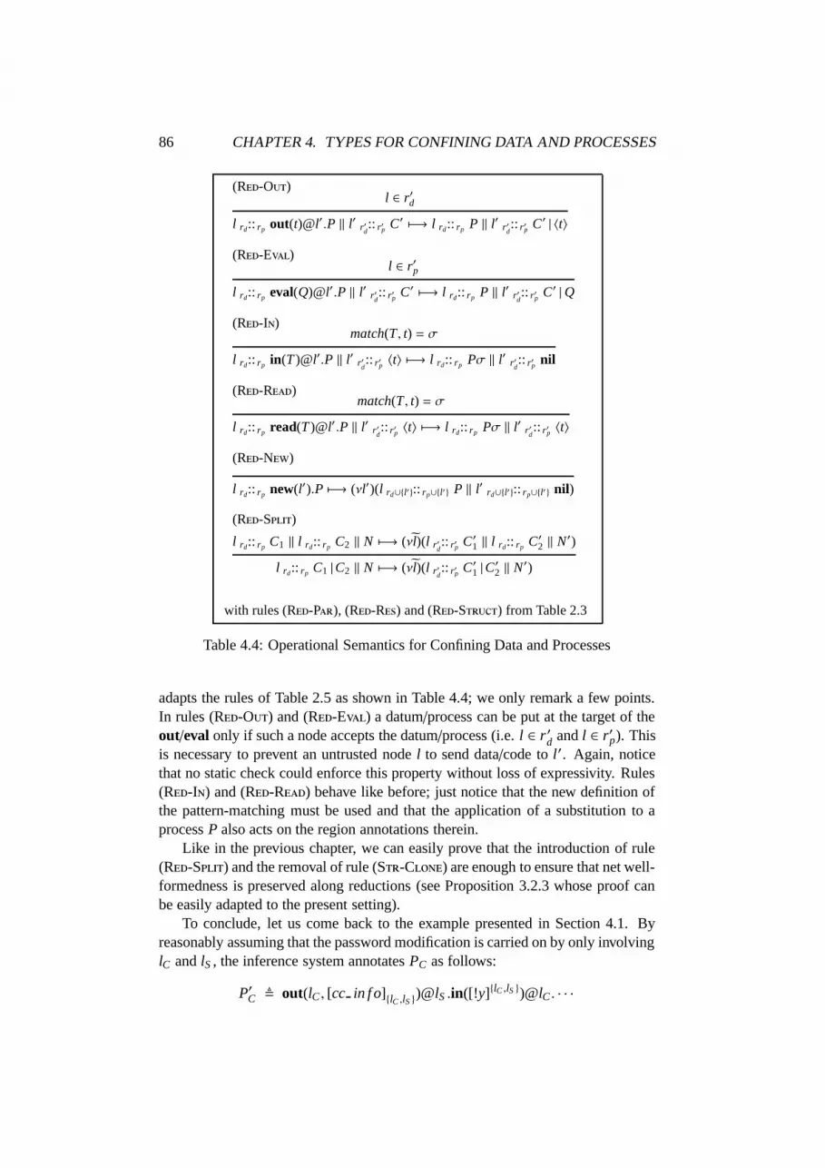
86 CHAPTER 4. TYPES FOR CONFINING DATA AND PROCESSES
(R-O)l ∈ r′d
l rd:: rp out(t)@l′.P ‖ l′ r′d:: r′p C′ 7−→ l rd:: rp P ‖ l′ r′d
:: r′p C′ | 〈t〉
(R-E)l ∈ r′p
l rd:: rp eval(Q)@l′.P ‖ l′ r′d:: r′p C′ 7−→ l rd:: rp P ‖ l′ r′d
:: r′p C′ |Q
(R-I)match(T, t) = σ
l rd:: rp in(T )@l′.P ‖ l′ r′d:: r′p 〈t〉 7−→ l rd:: rp Pσ ‖ l′ r′d
:: r′p nil
(R-R)match(T, t) = σ
l rd:: rp read(T )@l′.P ‖ l′ r′d:: r′p 〈t〉 7−→ l rd:: rp Pσ ‖ l′ r′d
:: r′p 〈t〉
(R-N)
l rd:: rp new(l′).P 7−→ (νl′)(l rd∪l′:: rp∪l′ P ‖ l′ rd∪l′:: rp∪l′ nil)
(R-S)
l rd:: rp C1 ‖ l rd:: rp C2 ‖ N 7−→ (νl)(l r′d:: r′p C′1 ‖ l rd:: rp C′2 ‖ N′)
l rd:: rp C1 |C2 ‖ N 7−→ (νl)(l r′d:: r′p C′1 |C
′2 ‖ N′)
with rules (R-P), (R-R) and (R-S) from Table 2.3
Table 4.4: Operational Semantics for Confining Data and Processes
adapts the rules of Table 2.5 as shown in Table 4.4; we only remark a few points.In rules (R-O) and (R-E) a datum/process can be put at the target of theout/eval only if such a node accepts the datum/process (i.e. l ∈ r ′d and l ∈ r′p). Thisis necessary to prevent an untrusted node l to send data/code to l′. Again, noticethat no static check could enforce this property without loss of expressivity. Rules(R-I) and (R-R) behave like before; just notice that the new definition ofthe pattern-matching must be used and that the application of a substitution to aprocess P also acts on the region annotations therein.
Like in the previous chapter, we can easily prove that the introduction of rule(R-S) and the removal of rule (S-C) are enough to ensure that net well-formedness is preserved along reductions (see Proposition 3.2.3 whose proof canbe easily adapted to the present setting).
To conclude, let us come back to the example presented in Section 4.1. Byreasonably assuming that the password modification is carried on by only involvinglC and lS , the inference system annotates PC as follows:
P′C , out(lC , [cc in f o]lC ,lS )@lS .in([!y]lC ,lS )@lC . · · ·

4.4. TYPE SOUNDNESS 87
Similarly, if we assume that credit card checking is performed locally by the serverand never used anymore, PS is annotated as:
P′S , rec X.in([!x1]lS , [!x2]lS )@lS . · · · .new(p).out([p]x1 ,lS )@x1. · · ·
Now, the dynamic checks of rule (R-I) are respected; thus, the resulting net canevolve as expected:
lC rCd:: rC
pP′C ‖ lS rS
d:: rS
pP′S
7−→ ∗ lC rCd:: rC
pin([!y]lC ,lS )@lC . · · · ‖
lS rSd:: rS
pP′S | < check cc in f o > .new(p).out([p]
lC ,lS )@lC . · · ·
7−→ ∗ lC rCd:: rC
p< modi f y password p and access the service > ‖
lS rSd:: rS
pP′S | < handle pwd modi f ications and
provide the service >
4.4 Type Soundness
Our main results state that well-typedness is preserved along reductions and thatwell-typed nets do respect region annotations. The proof of the first result, i.e.subject reduction, is similar to the corresponding proofs in the previous chapter;thus, we only highlight the differences. About the second result, i.e. safety, weneed a more sophisticated theory that we shall discuss with some details later on.
Lemma 4.4.1 (Subject Congruence) If N is well-typed and N ≡ N ′ then N′ iswell-typed.
Lemma 4.4.2 (Substitutivity) If Γ ] xi : rii ∈ I ` P u Γ′ ] xi : r′i i ∈ I ` P′
and σ = [li/xi]i ∈ I , then Γσ ` Pσ uσ Γ′σ ` P′σ .
Proof: Notice that it suffices to prove the claim for |I| = 1; indeed, a straightfor-ward induction on |I|, together with the fact that [li/xi]i=1,...,n = [l1/x1] . . . [ln/xn],can cover the more general case.
Thus, we consider only Γ] x : r ` P u Γ′] x : r′ ` P′ and we proceed
by induction on the length of the inference used to derive it. The base case is whenrules (T-N) or (T-D) are used: in both cases it is trivial to conclude. Letus consider the inductive case and reason by case analysis on the last rule used toinfer the judgement. We explicitly show the most significant case, i.e. when using(T-I); the remaining cases are similar or easier. By definition, P = in(T )@u′.Qand P′ = in(T ′)@u′.Q′, where Γ ] x : r ] y : uy ∈ bn(T ) ` Q u Γ
′′ ] x :r′′′ ] y : r′′y ∈ bn(T ) ` Q′ and T ′ is defined by (∗) in Table 4.2. By hypothesis,x < bn(T ); thus, by induction,
Γσ ] y : uσy ∈ bn(T ) ` Qσ uσ Γ′′σ ] y : r′′σy ∈ bn(T ) ` Q′σ

88 CHAPTER 4. TYPES FOR CONFINING DATA AND PROCESSES
Moreover, Γ′ = Γ′′bn(T ) and thus Γ′σ = (Γ′′bn(T ))σ = (Γ′′σ)bn(T ). Hence, byusing rule (T-I), we can conclude.
Theorem 4.4.3 (Subject Reduction) If N is well-typed and N 7−→ N ′, then N′ iswell-typed.
Proof: The proof proceeds by induction on the length of the inference. We onlyconsider the most peculiar cases.
(R-O). By hypothesis, N = l rd:: rp out(t)@l′.P ‖ l′ r′d:: r′p C′ and there exists a
net M such that M N. By definition, M = l rd:: rp out(t)@l′.Q ‖ l′ r′d:: r′p C′′
where ∅ ` out(t)@l′.Q l ∅ ` out(t)@l′.P and ∅ ` C′′ l′ ∅ ` C′ . Bythe premises of rule (T-O), ∅ ` Q l ∅ ` P and l′ ∈ r. This suffices toconclude that N′ = l rd:: rp P ‖ l′ r′d
:: r′p P′ | 〈t〉 is well-typed.
(R-I). By hypothesis, N results from the typing of a net M = l rd :: rp
in(T )@l′.Q ‖ l′ r′d:: r′p 〈t〉. By assuming that match(T, t) = σ, that must
hold because of the premise of rule (R-I), the main thing to prove isthat the well-typedness of l rd :: rp in(T )@l′.P implies the well-typedness ofl rd:: rp Pσ. By the premise of rule (T-I), it holds that
x : lx ∈ bn(T ) ` Q l x : rxx ∈ bn(T ) ` P
Hence, by Lemma 4.4.2, ∅ ` Q σ l ∅ ` P σ; this suffices to conclude.
(R-S). By hypothesis, we have that N = l rd :: rp C1|C2 ‖ N′′ results fromthe typing of a net M = l rd :: rp D1|D2 ‖ M′′. In particular, ∅ ` D1|D2 l
∅ ` C1|C2 that, by rule (T-P), implies that ∅ ` D1 l Γ ` C1 andΓ ` D2 l ∅ ` C2 . However, Γ must be ∅ as well; indeed, it can be easilychecked that Γ1 ` C l Γ2 ` C′ implies dom(Γ1) = dom(Γ2). Hence,l rd:: rp C1 ‖ l rd:: rp C2 ‖ N′′ is well-typed and, by induction, (νl)(l r′d
:: r′p C′1 ‖
l rd :: rp C′2 ‖ N′) is well-typed. This implies that (νl)(l r′d:: r′p C′1|C
′2 ‖ N′) is
well-typed, as required.
We now turn to type safety. As we have already said, it states that well-typedness guarantees absence of immediate violations of data regions. However,the wanted safety property requires that data regions are respected along all pos-sible computations. To properly formalise this property we need to define a finersemantics. Indeed, deeming a net to be safe when “for any node l rd :: rp P it holdsthat l occurs in the region of each datum in P” would not be satisfactory because theregions annotating data disappear upon data withdrawal. Thus, it would becomeimpossible to formalise the requirement that the region specification associated toa datum when it is produced is respected during all the datum life-time (i.e. alsoafter its retrieval). For example, consider the net
N = l rd:: rp in([!x]r′ )@l′.P ‖ l′ r′d:: r′p 〈[l
′′]r〉

4.4. TYPE SOUNDNESS 89
Upon execution of action in, the net becomes N ′ = l rd:: rp P′ ‖ l′ r′d:: r′p nil, where
P′ = P[l′′/x]. Now, the new occurrences of l′′ in P′ are not annotated anymore with
region r. Hence, in N′ we have no mean to formalise the statement that l can usel′′ by respecting the original annotation r.
To overcome this problem, we design a tagged language, where each occur-rence of a locality in a process is tagged with a region determining its visibility. Tothis aim, we slightly adapt the syntax of µK, by letting
u ::= [l]r
∣∣∣ x
We can now formalise when a net is safe. To this aim, we extend function regdefined in Section 4.2 by taking into account also the locality tags when calculatingthe region intersection. For example, reg(out([[l]r1
]r2)@[l′]r3
.P) = r1 ∩ r2 ∩ r3 ∩
reg(P).
Definition 4.4.4 (Safety) A net N is safe if, for any l rd :: rp C in N, it holds thatl ∈ reg(C).
The tagged operational semantics generalises that in Table 4.4; indeed, pro-cesses like out([[l]r1
]r2)@[l′]r3
or in([l]r1)@[l′]r2
can evolve. These terms mayarise upon application of substitutions that now map names into names tagged withregions. We let the application of the substitution to a region to replace names withplain names only (hence omitting their tags) thus ensuring that regions are still setsof names. The reduction relation, however, ignores the tags and considers taggednames as plain ones. This should have been somehow expected because, as we saidbefore, the only role of tags is to enable formalising and checking that a net is safe.To avoid confusion, we use the arrow 7−→→ to relate tagged terms.
The typing procedure for tagged terms is denoted by and its most significantrules are given in Table 4.5 (the other ones are smooth adaptations of those inTable 4.2). We use functions pid(u) and reg(u) to denote, respectively, the plainidentifier and the region of the tagged identifier u. The intuition underlying isthat, whenever an identifier occurs at a locality, the locality must be included in theregion tagging the identifier.
Given a plain net N, we use tag(N) to denote the set containing all the well-typed (w.r.t. ) tagged nets obtained by tagging localities in N. Given a taggednet N, we denote with untag(N) the plain net obtained from N by removing all thelocality tags. Notice that tag(N) is not empty because it contains at least the netobtained by tagging each locality in N with >. We call the latter net the outsettagging of N.
Predictably, the tagged language and the original one are strongly related.Moreover, the typing of tagged terms is preserved along (tagged) reductions. Thefollowing results formalise these properties.
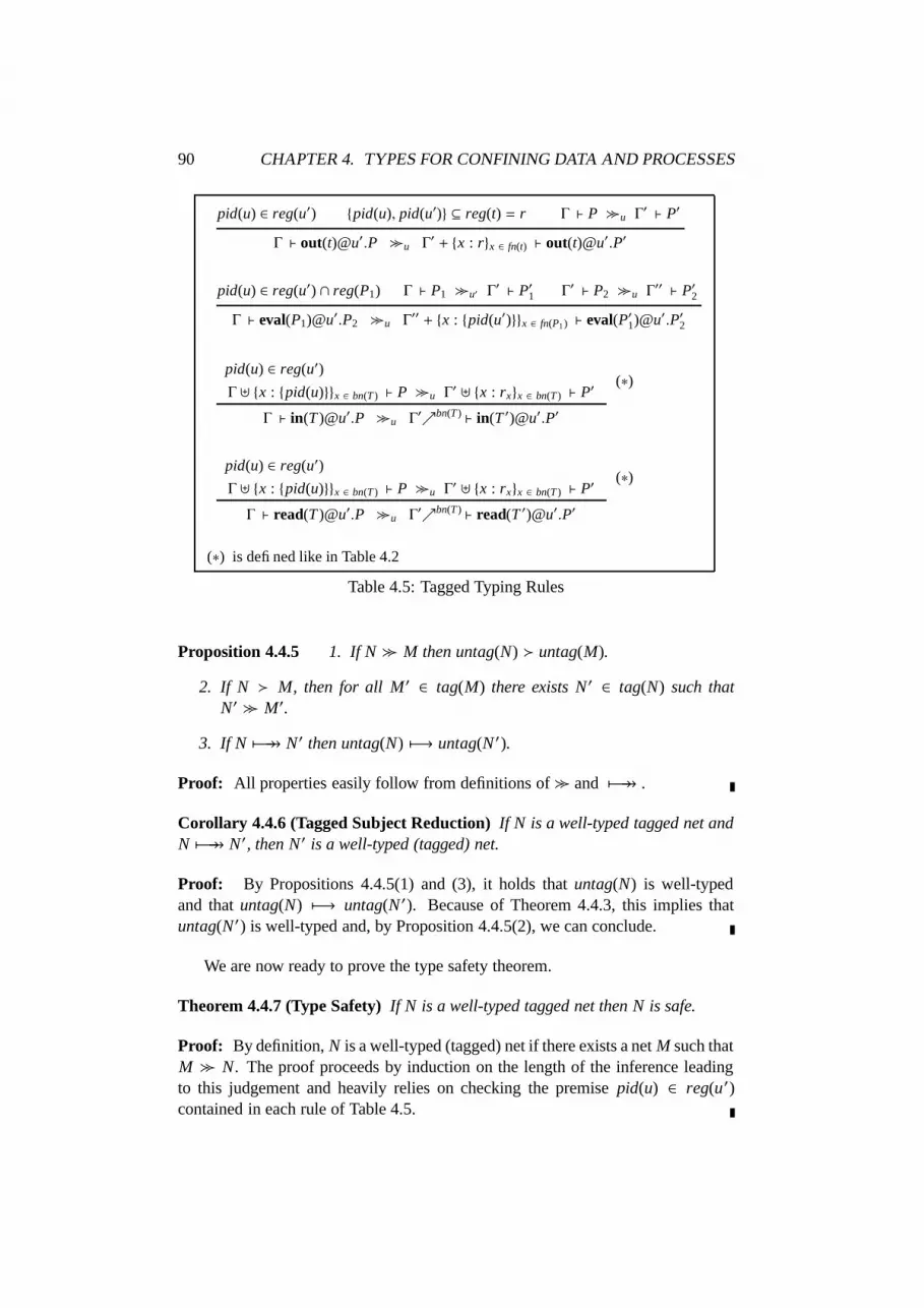
90 CHAPTER 4. TYPES FOR CONFINING DATA AND PROCESSES
pid(u) ∈ reg(u′) pid(u), pid(u′) ⊆ reg(t) = r Γ ` P u Γ′ ` P′
Γ ` out(t)@u′.P u Γ′ + x : rx ∈ fn(t) ` out(t)@u′.P′
pid(u) ∈ reg(u′) ∩ reg(P1) Γ ` P1 u′ Γ′ ` P′1 Γ′ ` P2 u Γ
′′ ` P′2
Γ ` eval(P1)@u′.P2 u Γ′′ + x : pid(u′)x ∈ fn(P1) ` eval(P′1)@u′.P′2
pid(u) ∈ reg(u′)
Γ ] x : pid(u)x ∈ bn(T ) ` P u Γ′ ] x : rxx ∈ bn(T ) ` P′
Γ ` in(T )@u′.P u Γ′bn(T ) ` in(T ′)@u′.P′
(∗)
pid(u) ∈ reg(u′)
Γ ] x : pid(u)x ∈ bn(T ) ` P u Γ′ ] x : rxx ∈ bn(T ) ` P′
Γ ` read(T )@u′.P u Γ′bn(T ) ` read(T ′)@u′.P′
(∗)
(∗) is defined like in Table 4.2
Table 4.5: Tagged Typing Rules
Proposition 4.4.5 1. If N M then untag(N) untag(M).
2. If N M, then for all M′ ∈ tag(M) there exists N′ ∈ tag(N) such thatN′ M′.
3. If N 7−→→ N′ then untag(N) 7−→ untag(N ′).
Proof: All properties easily follow from definitions of and 7−→→ .
Corollary 4.4.6 (Tagged Subject Reduction) If N is a well-typed tagged net andN 7−→→ N′, then N′ is a well-typed (tagged) net.
Proof: By Propositions 4.4.5(1) and (3), it holds that untag(N) is well-typedand that untag(N) 7−→ untag(N ′). Because of Theorem 4.4.3, this implies thatuntag(N′) is well-typed and, by Proposition 4.4.5(2), we can conclude.
We are now ready to prove the type safety theorem.
Theorem 4.4.7 (Type Safety) If N is a well-typed tagged net then N is safe.
Proof: By definition, N is a well-typed (tagged) net if there exists a net M such thatM N. The proof proceeds by induction on the length of the inference leadingto this judgement and heavily relies on checking the premise pid(u) ∈ reg(u′)contained in each rule of Table 4.5.

4.5. EXAMPLE: IMPLEMENTING A MULTIUSER SYSTEM 91
Corollary 4.4.8 (Type Soundness) Let N be a (plain) well-typed net and N ′ be itsoutset tagging. Then N′ 7−→→∗ N′′ implies that N′′ is safe.
Proof: By Proposition 4.4.5(2) and by the fact that N ′ ∈ tag(N), it holds that N′
is a well-typed tagged net. We now proceed by induction on the length of 7−→→∗.The base case is Theorem 4.4.7; the inductive case trivially follows by exploitingCorollary 4.4.6.
The results given above can be generalised by requiring only a subnet of thewhole net to be well-typed. By using the convention that absence of a regionannotation means >, a not well-typed net can be executed according to the (taggedversions of) rules in Table 4.4 by safely considering all its variable annotations as>. We call r-subnet of N the net formed by all the nodes l rd :: rp P in N such thatl∪ rd ∪ rp ⊆ r. Notice that such a net is not necessarily defined for all r; of courseit is always defined for r = > and coincides with N (in this case Theorem 4.4.9coincides with Corollary 4.4.8).
Theorem 4.4.9 (Localised Type Soundness) Let N be a plain net and N ′ be itsoutset tagging. If the r-subnet of N ′ is defined and well-typed, and if N ′ 7−→→∗N′′,then the r′-subnet of N′′ is defined and safe, where r′ = r ∪ L and L is the set ofnode addresses created during the computation.
Proof: By exploiting Theorem 4.4.7, we only need to show that the r ′-subnet ofN′′ is defined and well-typed. We just consider the case for N ′ 7−→→ N′′; the moregeneral case is recovered by using an inductive argument similar to that in Corol-lary 4.4.7. The proof proceeds like that of Theorem 4.4.3. Just notice that, whenthe operational rule used to infer the reduction is (the tagged version of) (R-O)or (R-E) resp., the premise l ∈ r′d or l ∈ r′p respectively turns out to be crucialto maintain well-typedness. Moreover, the only non trivial case for establishingif the r′-subnet is defined is when the operational rule used is (R-N). In thiscase, the claim is easily proved since the new node is assigned the regions of thecreating one.
To conclude, we want to remark that the language can be easily extended toenable explicit specification of the regions of the new nodes. In this case, existenceof the r′-subnet should be ensured by adding a premise to rule (R-N) requiringthat the regions of the new node are included in those of the creating node.
4.5 Example: Implementing a Multiuser System
In this section we use the framework presented so far to program a simple butmeaningful example. We present the behaviour of a simple UNIX-like multiusersystem, where users can login (exploiting a password-based approach) and usethe system functionalities, which consist in reading/writing files or executing pro-grams. For the sake of presentation, we shall present the system in three steps and,

92 CHAPTER 4. TYPES FOR CONFINING DATA AND PROCESSES
finally, we shall merge them together. Let lS be the address of the server, > be itsdata trust region and ∅ be its process trust region (thus no user can spawn code tolS ).
User Identification. We start with programming the identification of differentusers via passwords. Localities play the role of user IDs. Let lp be a private repos-itory used by lS to record the registered users and their passwords. Thus, lp hoststhe tuples
〈l1, [pwd1]l1,lp,lS 〉 | . . . | 〈ln, [pwdn]ln,lp,lS
〉
Let l be a user wanting to log in lS . If l is already known to lS (i.e. it is one ofthe lis), then l can use a process like
out(“login”, l, [pwd]l,lS )@lS .in(“logged”)@lS . . . .
for communicating with the server process
Login(lp) , rec X.in(“login”, !u, !z)@lS .(X |read(u, z)@lp.out([“logged”]
lS ,u)@lS )
Intuitively, l requires a connection by sending its user ID (its locality) and its pass-word; the server checks if this information is correct and sends back an ack, acti-vating the continuation of the computation at l. Notice that the region annotationsof pwd and “logged” rule out attacks of a nasty intruder aimed at cancelling therequest of login or the corresponding ack, and preserve the secrecy of the password.
If the user is not registered at lS yet, he can send an “hello” request to the servercontaining its address and wait for a password
out([“hello”]l,lS , l)@lS .in(“registered”, !pwd)@lS . . . .
The server then handles this request with the process
NewUser(lp) , rec X.in(“hello”, !u)@lS .(X |new(pwd).out(u, [pwd]
u,lS ,lp)@lp.
out(“registered”, [pwd]lS ,u
)@lS )
Of course, a locality l′ different from l can send to lS a request for a new passwordpretending to be l: the only difference with the “hello” message given above is thatthe message now should contain also l′ in the data region. However, the server willreport the new password to l and the region associated to the password will ensurethat pwd will not leave l. Thus, l′ cannot withdraw pwd: it can only try to send aprocess to l for acting at l with the new password. This can be possible only if ltrusts l′, implying that l accepts this ‘suspicious’ activity of l′.
We now show the use of our typing theory in the setting just presented. Inparticular, we give evidence of how we can prevent attacks aimed at cancellingmessages and activities of malicious users pretending to play the role of other users.

4.5. EXAMPLE: IMPLEMENTING A MULTIUSER SYSTEM 93
• Let lcanc be a locality hosting a process that aims at interfering with the lo-gin procedure above by performing action in(“hello”, !x)@lS . In this way,it removes the hello message sent by an unregistered user l willing to beconnected with the server lS . The system is modelled as follows
lcanc :: in(“hello”, !x)@lS .DONE ‖ lS :: NewUser(lp)‖ l :: out([“hello”]
l,lS , l)@lS .in(“registered”, !pwd)@lS . · · ·
7−→ lcanc :: in(“hello”, !x)@lS .DONE‖ l :: in(“registered”, !pwd)@lS . · · ·
‖ lS :: NewUser(lp) | 〈[“hello”]l,lS , l〉
7−→/ lcanc :: DONE ‖ l :: in(“registered”, !pwd)@lS . · · ·
‖ lS :: NewUser(lp)
Notice that the last transition cannot take place. As expected, the intruderrunning at lcanc is not enabled to withdraw the tuple 〈[“hello”]
l,lS , l〉 because
lcanc < l, lS (see the definition of pattern-matching in Table 4.3).
• Let now lpret be a locality pretending to act on behalf of l, by trying to acquirea log to lS under the identity of l. Let us examine the possible evolutions ofthe system:
lpret :: out(“hello”, l)@lS .in(“registered”, !pwd)@lS .DONE‖ lS :: NewUser(lp)
7−→7−→7−→7−→ lpret :: in(“registered”, !pwd)@lS .DONE‖ lS :: NewUser(lp)| 〈“registered”, [pwd]
lS ,l〉
7−→/ lpret :: DONE ‖ lS :: NewUser(lp)
Again, the last reduction cannot take place because lpret < lS , l.The only way for lpret to withdraw the tuple 〈“registered”, [pwd]
lS ,l〉
is to spawn a process to l (if it exists in the net) executing actionin(“registered”, !pwd)@lS (that would be enabled, because l ∈ lS , l). Sucha migration, however, should be authorised by l (indeed, it can take placeonly if lpret ∈ rl
p, where rlp is the node region controlling migrations to l).
The File System. We now consider a server handling a file system where differentusers can write/read data. Let l f be a private repository used by lS to store the files.A file named N, whose content is the string S , that can be read by users in r andwritten by users in r′, is stored in l f as the component
CN , 〈N , [“read”]r∪lS ,l f, [“written”]r′∪lS ,l f
〉∣∣∣ 〈N, S 〉
Intuitively, “read” and “written” are just dummy data used to properly store regionsr and r′. Then, the server handles requests for reading and writing files with the

94 CHAPTER 4. TYPES FOR CONFINING DATA AND PROCESSES
following processes
Read(l f ) , rec X.in(“read”, !u, !n)@lS .(X | read(n, !zr , !zw)@l f .
read(n, !z)@l f .out([zr]l f ,lS ,u, n, z)@u )
Write(l f ) , rec X.in(“write”, !u, !n, !z)@lS .(X | read(n, !zr , !zw)@l f .
in(n, !z′)@l f .out(n, z)@l f .out([zw]u,l f ,lS
, n)@u )
Intuitively, the first action in collects the request for reading/writing the file namedn performed by locality u; then the following read action, once type checked,verifies if the locality replacing u has the read/write privilege on file n (see below).Finally, the required operation is performed (the content of the file is read or theold content is replaced with the new one) and an acknowledgement (containing thekind of operation performed, the name of the file and, in the “read” case, also itscontent) is sent back to u.
We now show how our types can control read accesses to files. There are twofeatures devoted to this aim: the type inference phase carried on process Read(l f )and the runtime checks of the operational semantics (in particular, the premise ofrules (R-I) and (R-R)). We first give the type inference; recall that absenceof region annotations stands for >.
lS , u ⊆ s Γ1 ` nil lS Γ1 ` nil
Γ1 ` out ([zr]s, n, z)@u lS Γ2 ` out ([zr]s, n, z)@u
Γ3 ` read (n, !z)@l f .out([zr]s, n, z)@u lSΓ4 ` read (n, [!z]s)@l f .out([zr]s, n, z)@u
Γ5 ` read (n, !zr, !zw)@l f .read(n, !z)@l f .out([zr]s, n, z)@u lSΓ6 ` read (n, [!zr]s, [!zw]lS )@l f .read(n, [!z]s)@l f .out([zr]s, n, z)@u
∅ ` in (“read”, !u, !n)@l S .read(n, !zr, !zw)@l f .
read(n, !z)@l f .out([zr]s, n, z)@ulS ∅ ` in (“read”, [!u] ls, !n)@lS .read(n, [!zr]s, [!zw]lS )@l f .
read(n, [!z]s)@l f .out([zr]s, n, z)@u
where we let s , l f , lS , u and
Γ1 , Γ3 ] z : lS Γ2 , Γ1 + zr : s, n : s, z : sΓ3 , Γ5 ] zr : lS , zw : lS Γ4 , u : lS , n : s, zr : s, zw : lS Γ5 , u : lS , n : lS Γ6 , u : lS , n : s
We now call TRead(l f ) the process obtained from the typing inference above.Let l be a user wanting to read a file named FILE associated to a read regionρ = l f , lS , l, . . .. FILE is then stored at l f as the component
CFILE , 〈FILE , [“read”]ρ , [“written”]ρ′ 〉∣∣∣ 〈FILE, content〉

4.5. EXAMPLE: IMPLEMENTING A MULTIUSER SYSTEM 95
The evolution of user l is
l :: out(“read”, l, FILE)@lS .in(“read”, FILE, !cont)@l.P‖ l f :: CFILE ‖ lS :: TRead(l f )
7−→7−→ l :: in(“read”, FILE, !cont)@l.P ‖ l f :: CFILE
‖ lS :: TRead(l f ) | read(FILE, [!zr]l f ,lS ,l, [!zw]lS )@l f . · · ·
Now, action read(FILE, [!zr]l f ,lS ,l, [!zw]lS )@l f is enabled, because l f , lS , l is asubset of ρ; thus, the content of FILE will be transferred to l that, in turn, willbe enabled to retrieve it (by binding content to the variable cont) and use it in P.Notice that, if a user l′ < ρ had tried to carry on the same task, these actions wouldnot have been enabled, since l f , lS , l′ * ρ.
Executing Code-on-Demand. In this last setting, a user can dynamically down-load some code from the server to perform a given task. The server stores all thedownloadable processes as executable (named) files in a private locality lc. Foreach executable file named N, whose code is P and that is downloadable by nodesin r, the server stores in lc the component
CN , 〈N, [“downloaded”]r∪lS ,lc〉∣∣∣
rec X.in(req,N, !u)@lc .(X | read(N, !ze)@lc.eval( eval(out([ze]
lc,lS ,u,N)@u.P)@u )@lS )
Then, when a user wants to download some code, the server handles its requestwith the process
Execute(lc) , rec X.in(“execute”, !u, !n)@lS .out(req, n, u)@lc .X
Notice that lc cannot directly send P for execution to u because (the locality asso-ciated to) u cannot have lc in its trust region (since lc is fresh). Thus, P must firstlycross lS and then, if lS is in the process trust region of u (which we assume it is thecase), the code-on-demand procedure successfully terminates, by also reporting anack to the user.
The System. Finally, we can put together the activities shown so far to obtain theimplementation of the whole server. Thus, the (not yet typed) initial configurationof lS would be
lS > :: ∅ new(lp).new(l f ).new(lc) .< set up lp with the identites and passwords o f the users > .< set up l f with the data o f the f ile system > .< set up lc with the downloadable processes > .( NewUser(lp)
∣∣∣ Login(lp)∣∣∣ Read(l f )
∣∣∣Write(l f )
∣∣∣ Execute(lc) )
Our example simplifies UNIX behaviour in two major aspects: first, we did notrequire that a user must login before using the functionalities offered by the system;

96 CHAPTER 4. TYPES FOR CONFINING DATA AND PROCESSES
second, the files/programs are put by the system and not by the users. Both thesechoices were driven by the aim of simplifying the presentation, but our settingcould be easily enriched with more refined and realistic features.
Finally, we want to remark that, by exploiting the dummy data “downloaded”,“read” and “written”, we have been able to enforce an access control policy byonly using region annotations. This confirms that, in spite of its simplicity, theapproach we have presented in this chapter is very powerful.
4.6 Discussion and Related Work
In this chapter, we presented a programming notation aiming at protecting the se-crecy of both host and process data in global computing applications. By exploitinga preliminary compilation and some (unavoidable) runtime checks, we ensured thatdata can cross only nodes which are allowed to see them. The technique developedis good enough to assume only a local knowledge of the net during the compilationand work even when misbehaving entities are present in the system.
We want to remark that our theory permits to naturally implement a securitymechanism based on sandboxes. We already noticed that nodes can be seen aslogical partitions of a single physical machine. By exploiting this intuition, one cansplit each machine into an appropriate number of nodes each with its own securitypolicy. In this way, fine grained security policies can be programmed to guaranteethat untrusted processes (e.g., coming from unchecked nodes) are accepted onlyat dedicated nodes and that from these nodes remote operations and spawning ofthreads are not permitted.
The system we presented here is quite simple and easily implementable (typesare just sets and operations on types are unions, intersections, subset inclusions,...). Also its runtime semantics is reasonable, since it only involves efficientlyimplementable operations on sets. Moreover, by accepting more runtime checks,node regions could be handled more dynamically by defining primitives for addingand removing nodes from regions (in this way, e.g., nodes could choose whether totrust newly created ones). The problem is that, in this richer framework, none ofthe two guarantees illustrated at the beginning of Section 4.2 could be issued afterstatic checks. The type system would then only permit inferring the regions of thearguments of process actions, and render dynamic checks more efficient.
Related Work
Our work has been inspired by that on Confined-λ [98], a higher-order functionallanguage that supports distributed computing by allowing expressions at differentlocalities to communicate via channels. To limit the movement of values, program-mers can assign a type (i.e. a region) to them; a type system is defined that guaran-tees that each value can roam only within the allowed region. There are howeversome differences with our approach. First of all, we consider tuple spaces, another

4.6. DISCUSSION AND RELATED WORK 97
communication media that require a more dynamic typing mechanism. Then, wepermit annotating only the relevant data while in [98] a programmer must declarea type for any constant, function and channel. When typing a net, we do not relyon any form of global knowledge of the system; only the annotations in the processare considered. On the contrary, the type system in [98] assumes a global typingenvironment for handling shared channels; this somehow conflicts with the featuresof a global computing setting. Finally, we also give ‘localised’ formulations of thesoundness theorem stating that well-typedness of a given subnet is preserved alsoin presence of untyped contexts. This is a crucial property for global computingsystems where little assumptions on the behaviour of the context can be made.
The group types, originally proposed for the Ambients calculus [38] and thenrecast to the π-calculus [35], have purposes similar to our region annotations. Agroup type is just a name that can be dynamically created but cannot be commu-nicated (i.e. the scope of a group name cannot be extended). It permits to controlname visibility in different regions of a net: a fresh name belonging to a freshgroup can never be communicated to any process outside the scope of the group.Group types can then be used to handle processes and ambients movements, and ingeneral to prevent accidental or malicious leakage of private names without usingmore complex dependent types. However, differently from our approach, whenexploiting group types some global knowledge is still necessary for taking intoaccount the types of the names occurring free in a net.
Group types have also been used in region-based memory management wherethe focus is on efficiency, rather than on distribution and mobility. For instance, in[55] a connection between memory regions and group types is established and avariant of the π-calculus equipped with group types is used as a device to simplifythe proof of correctness of dynamic memory management.
Finally, we want to consider a lower level approach to protect visibility ofdata via encryption. Encrypted data can appear everywhere in the net, but can beeffectively used only by those users that know the decryption key. At an abstractlevel, we can consider the content of an encrypted message to be visible only withinthe region containing the nodes knowing the decryption key. Thus, it might appearthat our approach could be implemented by resorting to cryptographic primitives.However, we would like to stress an important difference. When encryption isused, the producer of encrypted data can control the access to (plain) data onlyby controlling visibility of the decryption key. But this can be hardly controlled:once a decryption key has been passed on, information leakage can reveal the key,thus breaking the controllability of data. By exploiting our approach, the dataproducer can decide in advance which are the users enabled to access the data; thisinformation is preserved during any evolution of the system. However, it shouldbe noticed that indirect information flows can be generated; for an account of theseproblems and some possible solutions we refer the interested reader to [84, 89].

98 CHAPTER 4. TYPES FOR CONFINING DATA AND PROCESSES

Chapter 5
Behavioural Theories
Programming computational infrastructures available globally for offering uniformservices has become one of the main issues in computer science, as we have largelyargued in the Introduction. On the foundational side, the demand is on the devel-opment of tools and techniques to build safer and trustworthy global systems, toanalyse their behaviour, and to demonstrate their conformance to given specifica-tions. Indeed, theoretical models and calculi can provide a sound basis for buildingsystems which are “sound by construction” and which behave in a predictable andanalysable manner. The crux is to equip the abstractions for global computers witheffective tools to support development and certification of global computing appli-cations.
Semantic theories, needed for stating and proving observable properties, shouldreflect all (or most of) the distinctive features of global systems at user’s applica-tion level; hence, they should ignore issues such as routing or network topology,because they are hardly observable at the user level.
In this chapter, we define some sensible semantics theories for µK and de-velop for them some tractable proof techniques. Given the direct correspondenceof µK with X-K, we believe that the tractable behavioural equivalenceswe develop here provide powerful tools to write sound programs for global com-puters. First, programs written in X-K are mapped down to µK; here theyare verified, by using behavioural equivalences to formalise and prove properties;finally, they can run on an actual global computer, like the Internet, by exploitingtheir Java-based translation [12].
We develop the semantic theories by defining behavioural equivalences overterms as the maximal congruences induced by some basic observables that aredictated by the relevant features of global computers. The approach can be sum-marised as follows:
1. Define a set of observables (values, normal forms, actual communications,. . . ) to which a term can evaluate by means of successive reductions.
2. Define a basic equivalence over terms by stating that two terms are equivalentif and only if they exhibit the same set of basic observables.
99

100 CHAPTER 5. BEHAVIOURAL THEORIES
3. Consider the largest congruence over the language induced by the basicequivalence or by its co-inductive closure.
A similar approach has already been used to study models of concurrent systems(e.g., CCS [115, 15] and π-calculus [133, 5]). Obviously, the designation of thebasic observables is critical. Thus, we draw inspiration from everyday experience:a user can observe the behaviour of a global computer (at the application level) bytesting
i. whether a specific site is up and running (i.e., it provides some data of anykind),
ii. whether a specific information is present in (at least) a site, or
iii. whether a specific information is present in a specific site.
Other calculi for global computers rely on (barbed) congruences induced by similarobservables: for example, Ambient [41] uses a barb that is somehow related to i.above, while the barbs in Dπ-calculus [85] are strongly related to iii. .
A question that naturally arises is whether these observables yield ‘interesting’congruences. The three basic observables, together with the discriminating powerprovided by µK contexts, all yield the same congruence, when used similarly.This is for us already an indication of the robustness of the resulting semantic the-ories. Moreover, as we will show, the observables are still sufficiently powerfulto give rise to interesting semantic theories also when considering lower-level fea-tures like, e.g., failures. Due to its intuitive appeal, in the rest of this chapter weshall mainly use the first kind of observable.
A major drawback of the approach relying on basic observables and contextclosures is that the resulting congruences are defined via universal quantificationover all language contexts, and this makes their checking very hard. It is then im-portant to devise proof techniques that avoid such quantification. We shall define alabelled transition system (with labels indicating the performed action) and exploitthe labels to avoid quantification over contexts. We shall present tractable charac-terisations of two ‘touchstone’ congruences, namely barbed congruence and maytesting, in terms of (non-standard) labelled bisimilarity and trace equivalence, re-spectively. In doing this, we have to face the problems raised by the presence ofexplicit localities and by the fact that µK is asynchronous (both in the com-munication and in the mobility paradigm) and higher-order (because processes canmigrate).
5.1 Touchstone Equivalences
In this section we present (weak) equivalences yielding sensible semantic theoriesfor µK. The approach we follow relies on the definition of an observation(also called barb) that intuitively formalises the possible interactions of a process.

5.1. TOUCHSTONE EQUIVALENCES 101
We use observables to define equivalence relations that identify those nets thatcannot be taken apart by any basic observation after any reduction in any context.Notationally, we shall use |=⇒ to denote the reflexive and transitive closure of 7−→.
Definition 5.1.1 (Barbs and Contexts)Predicate N ↓ l holds true if and only if N ≡ (νl)(N′ ‖ l :: 〈t〉) for some l, N′
and t such that l < l.Predicate N ⇓ l holds true if and only if N |=⇒ N ′ for some N′ such that N′ ↓ l.A context C[·] is a µK net with an occurrence of a hole [·] to be filled in
with any net. Formally,
C[·] ::= [·]∣∣∣ N ‖ C[·]
∣∣∣ (νl)C[·]
We have chosen the basic observables by taking inspiration from those used forthe asynchronous π-calculus [5]. One may wonder if our choice is “correct” andargue that there are other alternative notions of basic observables that seem quitenatural, as we have discussed before. A first alternative could be to consider asequivalent two nets if they make available the same set of data, possibly in differentnodes (this choice can be defended as follows: when a user looks for a paper in theweb he may not be interested whether he finds the paper in author’s web pages or inpublisher’s one). A second alternative could be to consider as equivalent two nets ifthey have exactly the same data at the same localities. Later on, we shall prove thatthe congruences induced by these alternative observables do coincide. This meansthat our results are quite independent from the observable chosen and vindicatesour choice. Moreover, notice that, by using other kinds of observation predicates,more sophisticated equivalences should come into the picture. For example, in[15] it is shown how must testing and fair testing can be obtained in CCS by onlychanging the basic observable.
Now, we say that a binary relation < between nets is
• barb preserving, if N<M and N ⇓ l imply M ⇓ l;
• reduction closed, if N < M and N 7−→ N ′ imply M |=⇒ M′ and N′ < M′,for some M′;
• context closed, if N < M implies C[N]< C[M] for every context C[·].
Our touchstone equivalences should at the very least relate nets with the same ob-servable behaviour; thus, they must be barb preserving. However, an equivalencedefined only in terms of this property are too weak: indeed, the set of barbs changesduring computations or when interacting with an external environment. Moreover,for the sake of compositionality, our touchstone equivalences should also be con-gruences. These requirements lead us to the following definitions.
Definition 5.1.2 (May testing) ' is the largest symmetric, barb preserving andcontext closed relation between nets.

102 CHAPTER 5. BEHAVIOURAL THEORIES
Definition 5.1.3 (Barbed congruence) is the largest symmetric, barb preserv-ing, reduction and context closed relation between nets.
We want to remark that the above definition of barbed congruence is the standardone, see [96, 124]. May testing is, instead, usually defined in terms of observers,experiments and possible successes of experiment [65]. However, if we let '′ de-note the equivalence on µK nets defined a la [65], we can prove that the twodefinitions do coincide. Moreover, the inclusions between our touchstone equiv-alences reflect the inclusions that hold in the π-calculus. To define may testinglike in [65], we let test be a fresh and reserved name used to report success ofan experiment (i.e. a computation) of a net and an observer. The latter is a netcontaining (i) a node whose address is test that can only host the datum 〈test〉,and (ii) processes that may emit the datum 〈test〉 at test. A computation reportssuccess if, along its execution, a datum 〈test〉 at node test appears; this is writtenOK===⇒ .
Definition 5.1.4 N '′ M if, for any observer K, it holds that N ‖ KOK===⇒ if and
only if M ‖ KOK===⇒ .
Proposition 5.1.5 ⊂ ' = '′.
Proof: That is a sub-relation of ' trivially follows from their definitions.The inclusion is strict because the latter equivalence abstracts from the branchingstructure of the equated nets, while the former one does not (because of reductionclosure). This is standard in process calculi, e.g., in CCS and in π-calculus.
We start proving that ' ⊆ '′ . Let N ' M and pick up any observer K such that
N ‖ KOK===⇒ . Then, by contextuality, N ‖ K ' M ‖ K and, by barb preservation,
N ‖ K ⇓ test (that comes from N ‖ KOK===⇒ ) implies that M ‖ K ⇓ test.
Since test is a name occurring only in K (by definition of observers), it must be
M ‖ KOK===⇒ , as required.
Viceversa, we need to prove that '′ is barb preserving and context closed. LetN '′ M.
Barb preservation. Let N ⇓ l, i.e. N |=⇒ (νl)(N′ ‖ l :: 〈t〉) and consider K ,test :: in(T )@l.out(test)@test, where T is a template matching against
t and such that fn(T ) ∩ l = ∅. Then, N ‖ KOK===⇒ that, by hypothesis, implies
M ‖ KOK===⇒ . Now, because of freshness of test, this is possible only if
M ⇓ l.
Context closure. The proof is by induction on the structure of the context C[·].The base case is trivial. For the inductive case, we have two possibilities:
• C[·] , D[·] ‖ H. By induction, D[N] '′ D[M]; we pick up an
observer K and prove that C[N] ‖ KOK===⇒ implies C[M] ‖ K
OK===⇒

5.1. TOUCHSTONE EQUIVALENCES 103
(by symmetry, this suffices). We now consider the observer H ‖ K; by
Definition 5.1.4, by induction and by the fact thatD[N] ‖ (H ‖ K)OK===⇒
we have that D[M] ‖ (H ‖ K)OK===⇒ . The thesis easily follows by rule
(S-PA) and because ≡ ⊆ '′.
• C[·] , (νl)D[·]. By induction, D[N] '′ D[M]; we pick up an observer
K and we prove that C[N] ‖ KOK===⇒ implies C[M] ‖ K
OK===⇒ . Since
l is bound, we can assume, up-to alpha-equivalence, that l < fn(K); in
particular, l , test. Now, C[N] ‖ KOK===⇒ if and only if D[N] ‖
KOK===⇒ (and similarly when replacing N with M). This suffices to
conclude.
Traditionally [146, 147], barbed congruence and may testing are, respectively,the bottom and the top element of the lattice induced by the subset inclusion be-tween (weak) equivalences on a given process calculus. Practically all the inter-esting weak equivalences that have been developed in process calculi fall betweenthese two kinds of equivalences. Moreover, a part from the theorical interest, itis worth to study both these equivalences because the former one enjoys a moreeffective proof technique, while the latter one often sufficies to express propertiesof programs (mainly, those properties that can be expressed in terms of reachabil-ity of a particular state). Hence, we do not have any preference among these twoequivalences and we consider both of them as a benchmark for µK.
The problem behind the definition of barbed congruence and may testing is thatcontext closure makes it hard to prove equivalences due to the universal quantifica-tion over contexts. In the following sections, we shall provide two tractable char-acterisations of these equivalences, as a bisimulation-based and as a trace-basedequivalence.
Before doing this, we show that we can change observables without changingthe congruences they induce; this proves the robustness of our touchstone equiv-alences and supports our choice. Other two reasonable observables in a globalcomputing framework can be existence of a specific (visible) datum in some nodeof a net, or existence of a specific datum in a specific node of a net.
Definition 5.1.6 (Alternative Touchstone Equivalences) Let 1, 2 '1 and '2
be the reduction barbed congruences and the may testing equivalences obtainedby replacing the observable of Definition 5.1.1, respectively, with the followingones:
1. N ↓ 〈t〉 iff N ≡ (νl)(N′ ‖ l :: 〈t〉) for some l and l such that l, t ∩ l = ∅
2. N ↓l 〈t〉 iff N ≡ (νl)(N′ ‖ l :: 〈t〉) for some l such that l, t ∩ l = ∅
We now prove that, thanks to contextuality, 1 and 2 coincide with , and that '1
and '2 coincide with '.

104 CHAPTER 5. BEHAVIOURAL THEORIES
Proposition 5.1.7 1 = 2 = and '1 = '2 = '.
Proof: Notice that we only need to consider barb preservation. Indeed, contex-tuality and reduction closure (in the case of barbed congurence) are ensured bydefinition. We just work with barbed congruences; the proofs for may testing canbe then extracted straightforwardly.
2 ⊆ 1. Let N 2 M. Suppose that N ⇓ 〈t〉. This implies that ∃ l : N ⇓l 〈t〉.Hence, by hypothesis, M ⇓l 〈t〉 that, by definition, implies M ⇓ 〈t〉.
1 ⊆ . Let N 1 M and N ⇓ l, i.e. N |=⇒ (νl)(N′ ‖ l :: 〈t〉). Then M ⇓ l, otherwisethe context [·] ‖ l′ :: in(T )@l.out(l′)@l′ (for l′ fresh and T matching againstt such that fn(T ) ∩ l = ∅) would break 1.
⊆ 2. This case is similar.
5.2 Bisimulation Equivalence
To coinductively capture barbed congruence, we introduce a labelled transitionsystem (LTS) to make apparent the action a net is willing to perform in order toevolve. For the sake of presentation, we introduce the syntactic category of inertcomponents
I ::= nil∣∣∣ 〈t〉
for grouping those components that are unable to perform any basic operation. The
labelled transition relation,α−→ , is defined as the least relation over nets induced
by the inference rules in Table 3.8. Transition labels take the form
χ ::= τ∣∣∣ (νl) I @ l α ::= χ
∣∣∣ . l∣∣∣ t / l
We will write bn(α) for l if α = (νl) I @ l and for ∅, otherwise; fn(α) is definedaccordingly.
Let us now briefly comment on some rules of the LTS; most of them are adaptedfrom the π-calculus [124]. Rule (LTS-E) signals existence of nodes (labelnil @ l ) or of data (label 〈t〉 @ l). Rules (LTS-O) and (LTS-E) express theintention of spawning a component and require the existence of the target nodeto complete successfully (rule (LTS-S)). Similarly, rules (LTS-I) (given inan early style) and (LTS-R) express the intention of performing an input; thisinput is actually performed (rule (LTS-C)) only if the chosen datum is presentin the target node. Notice that, in the right hand side of these rules, existence ofthe node target of the action can be assumed: indeed, if l provides datum 〈t〉, thisimplies that l does exist. Rule (LTS-O) signals extrusion of bound names; as insome presentation of the π-calculus, this rule is used to investigate the capability ofprocesses to export bound names, rather than to extend the scope of bound names.To this last aim, law (S-E) is used; in fact, in rule (LTS-C) labels do not

5.2. BISIMULATION EQUIVALENCE 105
(LTS-O)
l :: out(t)@l′.P. l′−−→ l :: P ‖ l′ :: 〈t〉
(LTS-E)
l :: eval(Q)@l′.P. l′−−→ l :: P ‖ l′ :: Q
(LTS-I)match(T, t) = σ
l :: in(T )@l′.Pt / l′−−−→ l :: Pσ ‖ l′ :: nil
(LTS-R)match(T, t) = σ
l :: read(T )@l′.Pt / l′−−→ l :: Pσ ‖ l′ :: 〈t〉
(LTS-N)
l :: new(l′).Pτ−→ (νl′)(l :: P ‖ l′ :: nil)
(LTS-E)
l :: II @ l−−−→ l :: nil
(LTS-C)
N1t / l′−−−→ N′1 N2
〈t〉 @ l′−−−−−→ N′2
N1 ‖ N2τ−→ N′1 ‖ N′2
(LTS-S)
N1. l−→ N′1 N2
nil @ l−−−−−→ N′2
N1 ‖ N2τ−→ N′1 ‖ N′2
(LTS-R)
Nα−→ N′ l < n(α)
(νl)Nα−→ (νl)N′
(LTS-O)
N(νl) 〈t〉 @ l′
−−−−−−−→ N′ l ∈ fn(t) − l, l′
(νl)N(νl,l) 〈t〉 @ l′
−−−−−−−−→ N′
(LTS-P)
N1α−→ N2 bn(α) ∩ fn(N) = ∅
N1 ‖ Nα−→ N2 ‖ N
(LTS-S)
N ≡ Mα−→ M′ ≡ N′
Nα−→ N′
Table 5.1: µK Labelled Transition System (LTS)
carry any restriction on names, whose scope must have been previously extended.Rules (LTS-R), (LTS-P) and (LTS-S) are standard.
To simplify the proofs, we consider a slightly extended structural congruence:it is defined like in Table 2.2 (with the obvious adaption of K nodes to µKones) plus the rule
(S-RN) (νl)N ≡ (νl)(N ‖ l :: nil)
saying that any restricted name can be used as the address of a node1. In whatfollows, we shall only consider nets where each bound name is associated to anode; by virtue of rule (S-RN) this is always possible. This is necessary,otherwise our semantic theories would distinguish names restricted at the outset
1Restricted names can be thought of as private network addresses, whose corresponding nodescan be activated when needed, and successively deactivated, by the owners of the resource (i.e. thenodes included in the scope of the restriction).
Moreover, notice that we did not included this rule from the beginning (i.e., in Table 2.2) becauseit would have created problems when dealing with types: the type of a restricted node derives fromthe type of its creator and rule (S-RN) does not keep this information into account.

106 CHAPTER 5. BEHAVIOURAL THEORIES
from those created during computations: the former ones are not necessarily theaddress of a node, while the latter ones are (see rules (R-N) and (LTS-N)).
Notation 5.2.1 We shall write Nα−→ to mean that there exists a net N ′ such that
Nα−→ N′. Alternatively, we could say that N can perform a α-step. Moreover, we
shall usually denote relation composition by juxtaposition; thus, e.g., Nα−→α′
−→ M
means that there exists a net N ′ such that Nα−→ N′
α′
−→ M. We shall use the conven-tion that putting a bar over a relation means that such a relation does not hold (e.g.
N 6α−→ N′ means that N cannot reduce to N ′ performing α). As usual, we let =⇒ to
stand forτ−→∗,α=⇒ to stand for =⇒
α−→ =⇒ , and
α=⇒ to stand for =⇒ , if α = τ, and
forα=⇒ , otherwise.
The LTS we have just defined is ‘correct’ w.r.t. the operational semantics ofµK, as stated by the following Proposition. Notice that 7−→ is the actual se-mantics of µK; the LTS of Table 5.1 can be thought of as a technical devicedeployed to give a tractable formulation of barbed congruence.
Proposition 5.2.2 N 7−→ M if and only if Nτ−→ M.
Proof: Both the directions are proved by an easy induction on the lenght of theshortest inference leading to the judgements.
Now, we prove some relationships between transitions of the LTS and the syntac-tical form of the net performing them.
Proposition 5.2.3 The following facts hold:
1. Nnil @ l−−−−−→ N′ if and only if N ≡ N′′ ‖ l :: nil; moreover, N′′ ≡ N′ ≡ N.
2. N(νl) 〈t〉 @ l−−−−−−−→ N′ if and only if N ≡ (νl)(N′′ ‖ l :: 〈t〉) for l < l; moreover,
N′ ≡ N′′ ‖ l :: nil.
Proof: In both statements, the ‘if’ part is straightforward, by using (LTS-E)and (LTS-S)/(LTS-P)/(LTS-O)/(LTS-R). For the converse, the firstclaim is proved by a straightforward induction on the inference. The second claimis proved in a slightly more elaborated way. Indeed, we need a double induction:one on the cardinality of l, and the other on the inference length. We leave thedetails to the reader.
We now characterise barbed congruence by using the labels of the LTS insteadof the universal quantification over all contexts. In this way, we obtain an alterna-tive characterisation of in terms of a labelled bisimilarity.

5.2. BISIMULATION EQUIVALENCE 107
Definition 5.2.4 (Bisimilarity) A symmetric relation < between µK nets is a(weak) bisimulation if for each N < M it holds that:
1. if Nχ−→ N′ then, for some M′, M
χ=⇒ M′ and N′ < M′;
2. if N. l−→ N′ then, for some M′, M ‖ l :: nil =⇒ M′ and N′ < M′;
3. if Nt / l−−→ N′ then, for some M′, M ‖ l :: 〈t〉 =⇒ M′ and N′ < M′.
Bisimilarity, ≈, is the largest bisimulation.
Our bisimulation is somehow inspired by that in [119]. The key idea is that,
since sending operations are asynchronous, the evolution N. l−→ N′ can be simu-
lated by a net M (in a context where locality l is present) through execution ofsome internal actions that lead to M′. Indeed, since we want our bisimulation to bea congruence, a context that provides the target locality of the sending action mustnot tell apart N and M. Hence, for N ‖ l :: nil to be simulable by M ‖ l :: nil,it must hold that, upon transitions, N ′ be simulable by M′. Similar considerationshold also for input actions (third item of Definition 5.2.4), but the context now is[·] ‖ l :: 〈t〉.
Remarkably, though µK is higher order (processes occur as arguments inprocess actions, namely in the eval), the LTS and the bisimulation we developeddo not use labels containing processes. Thus, the bisimulation relies only on astandard quantification over names (in the input case) and we strongly conjecturethat it is decidable, under proper assumptions: techniques similar to those in [116]could be used here. Moreover, the presence of rule (LTS-S) in the LTS doesnot compromise the tractability of ≈: as standard, (LTS-S) can be dropped,once we accept to have more rules in the LTS.
5.2.1 Soundness w.r.t. Barbed Congruence
The key result of this subsection is Lemma 5.2.7 that will easily allow us to con-clude that bisimilarity is a sound proof technique for barbed congruence. To provethis result, we need some technical tools. First of all, we introduce the notion ofbisimulation up-to structural congruence: it is defined as a labelled bisimulationexcept for the fact that the < in the consequents of Definition 5.2.4 is replaced bythe relation ≡ < ≡. Lemma 5.2.5 shows that a bisimulation up-to ≡ is a bisimula-tion. Then, Lemma 5.2.6 characterises all the possible executions of the net C[N]in terms of the evolutions of N and C[·] separately.
Lemma 5.2.5 If N ≈ M then for any nets N ′ and M′ such that N ≡ N′ andM ≡ M′ it holds that N′ ≈ M′.
Proof: Let < , (N1,N2) : Ni ≡ N′i and N′1 ≈ N′2 . We shall prove that
< is a labelled bisimulation. Let N1α−→ M1; by (LTS-S) we have that N ′1 ≡

108 CHAPTER 5. BEHAVIOURAL THEORIES
N1α−→ M1. We only consider the case for α = χ; the other cases are similar. By
hypothesis, N′2χ−→ M2 for some M2 such that M1 ≈ M2. Then, N2 ≡ N′2
χ=⇒ M2 and
(M1,M2) ∈ < because of reflexivity of ≡.
Lemma 5.2.6 C[N]α−→ N if and only if one of the following conditions hold:
1. Nα−→ N′ with n(α) ∩ bn(C[·]) = ∅, or
2. C[0]α−→ C′[0], or
3. N(νl) 〈t〉 @ l−−−−−−−→ N′ with α = (νl′, l) 〈t〉 @ l , C[·] , C1[(νl′)C2[·]] and fn(α) ∩
bn(C1[·],C2[·]) = ∅, or
4. C[·] , C1[C2[·] ‖ H] with Hnil @ l−−−−−→ H′, N
. l−→ N′ and l < bn(C2[·]), or
5. C[·] , C1[C2[·] ‖ H] with H. l−→ H′, N
nil @ l−−−−−→ N′ and l < bn(C2[·]), or
6. C[·] , C1[C2[·] ‖ H] with H(νl) 〈t〉 @ l−−−−−−−→ H′, N
t / l−−→ N′ and l, t ∩ bn(C2[·]) =
∅, or
7. C[·] , C1[C2[·] ‖ H] with Ht / l−−→ H′, N
(νl) 〈t〉 @ l−−−−−−−→ N′ and l < bn(C2[·])
Moreover, the resulting net N is, respectively, structurally equivalent to C[N ′], orC′ [N], or C1[C2[N′]], or C[N′], or C1[C2[N] ‖ H′], or C1[(νl)C2[N′ ‖ H′]] (cases6 and 7.). Finally, α = τ in cases 4., 5., 6., and 7. .
Proof: The “if” part is trivial, by using the LTS of Table 5.1 and by observing that
Mα−→ M′ with n(α) ∩ bn(D[·]) = ∅ implies D[M]
α−→D[M′]. The “only if” part is
proved by induction on the length of the inference ofα−→ . In the base case (length
1), it must be C[·] , [·]; hence, obviously C[N] , Nα−→ N′ , C[N′] (and hence we
fall in case 1. of this Lemma). For the inductive step, we reason by case analysison the last rule applied in the inference:
(LTS-R). In this case, it must be
D[N]α−→ N′ l < n(α)
C[N] , (νl)D[N]α−→ (νl)N′
We can now apply induction and reason by analysis on the used case of thislemma.
1. Nα−→ N′, n(α) ∩ bn(D[·]) = ∅ and N′ ≡ D[N′]. Hence, we still fall in
case 1. by using the context C[·] , (νl)D[·].
2. D[0]α−→D′ [0] and N′ ≡ D′[N]. Hence, we still fall in case 2. with
contexts C[·] , (νl)D[·] and C′[·] , (νl)D′ [·].

5.2. BISIMULATION EQUIVALENCE 109
3. N(νl) 〈t〉 @ l′−−−−−−−−→ N′, α , (νl′, l) 〈t〉@ l′ ,D[·] , D1[(νl′)D2[·]] and n(α)∩
bn(D1[·],D2[·]) = ∅; moreover, N′ ≡ D1[D2[N′]]. Hence, we still fallin case 3. by using the contexts C1[·] , (νl)D1[·] and C2[·] , D2[·].
4. D[·] , D1[D2[·] ‖ H] with Hnil @ l−−−−−→ H′, N
. l−→ N′ and l < bn(D2[·]);
moreover, D[N]τ−→D[N′]. Hence we still fall in case 4. by using the
contexts C1[·] , (νl)D1[·] and C2[·] , D2[·].
5. 6. and 7. are similar.
(LTS-O). In this case, it must be
D[N](νl) 〈t〉 @ l−−−−−−−→ N l′ ∈ t − l, l
C[N] , (νl′)D[N](νl′ ,l) 〈t〉 @ l−−−−−−−−−→ N
We can now apply induction and reason by analysis on the used case of thislemma; we have to consider only the first three cases.
1. N(νl) 〈t〉 @ l−−−−−−−→ N′, l, t ∩ bn(D[·]) = ∅ and N , D[N′]. Hence, we fall in
case 3. by using the contexts C1[·] , [·] and C2[·] , D[·].
2. D[0](νl) 〈t〉 @ l−−−−−−−→D′ [0] and N , D′[N]. Hence, we still fall in case 2.
with contexts C[·] , (νl2)D[·] and C′ [·] , D′ [·].
3. N(νl1) 〈t〉 @ l−−−−−−−−→ N′, D[·] , D1[(νl2)D2[·]], l = l1, l2 and t, l ∩
bn(D1[·],D2[·]) = ∅; moreover, N , D1[D2[N′]]. Hence, we stillfall in case 3. by using the contexts C1[·] , [·] and C2[·] , D[·].
(LTS-P). In this case, one of the following inferences should hold:
Kα−→ K′ bn(α) ∩ n(D[N]) = ∅
C[N] , D[N] ‖ Kα−→ D[N] ‖ K′
orD[N]
α−→ N′ bn(α) ∩ n(K) = ∅
C[N] , D[N] ‖ Kα−→ N′ ‖ K
By using the first inference, we fall in case 2. with resulting context C′ [·] ,D[·] ‖ K′. By using the second inference, we can apply inductive argumentssimilar to those used in the (LTS-R) case, but now the context C[·] weconsider is D[·] ‖ K instead of (νl)D[·].
(LTS-S). In this case, one of the following inferences should hold:
K. l−→ K′ D[N]
nil @ l−−−−−→D[N]
C[N] , D[N] ‖ Kτ−→ D[N] ‖ K′
orK
nil @ l−−−−−→ K D[N]
. l−→ N′
C[N] , D[N] ‖ Kτ−→ N′ ‖ K
To apply induction, notice that we only have to consider the first two casesof this lemma, since the actions fired by D[N] are different from τ and haveno restricted names. For the first reduction, we have the following cases.

110 CHAPTER 5. BEHAVIOURAL THEORIES
1. Nnil @ l−−−−−→ N and l < bn(D[·]). Hence, we fall in case 5. by using
C1[·] , [·], C2[·] , D[·] and H , K.
2. D[0]nil @ l−−−−−→D[0]; hence, we still fall in case 2. with resulting context
C′[·] , D[·] ‖ K′.
For the second reduction, we have similar cases; we just list the differences.
1. N′ , D[N′] and we fall into case 4. .
2. N′ , D′ [N] and the resulting context is C′[·] , D′[·] ‖ K.
(LTS-C). In this case, one of the following inferences should hold:
D[N]t / l−−→ N′ K
〈t〉 @ l−−−−−→ K′
C[N] , D[N] ‖ Kτ−→ N′ ‖ K′
or Kt / l−−→ K′ D[N]
〈t〉 @ l−−−−−→ N′
C[N] , D[N] ‖ Kτ−→ N′ ‖ K′
Like before, we just have two possible inductive cases for each reduction(namely, the first two of this lemma). For the first reduction we have thefollowing cases.
1. Nt / l−−→ N′, l, t∩bn(D[·]) = ∅ and N′ , D[N′]. Hence, we fall in case
6. by using C1[·] , [·], C2[·] , D[·] and H , K.
2. D[0]t / l−−→D′ [0] and N′ , D′ [N]. Hence, we still fall in case 2. with
resulting context C′[·] , D′ [·] ‖ K′.
For the second reduction, we have similar cases. The only difference is thatcase 1. in the induction leads to case 7. in the conclusion.
(LTS-S). In this case, it must be
C[N] ≡ M1α−→ M2 ≡ N
C[N]α−→ N
We now proceed by induction on the structure of context C[·]. The base case(for C[·] , [·]) trivially falls in case 1. of this Lemma. For the inductivecase, let us reason by case analysis on the structure of C[·]:
C[·] , (νl)D[·]. We furtherly identify three possible sub-cases:
• if M1 , (νl)M and l ∈ bn(α), for some M ≡ D[N], then we can
apply the structural induction to D[N]α′
−→ M′, for some M′ ≡ M2
and α = (νl)α′, and fall in one of the first two cases of this Lemma.By using rule (LTS-O), we can conclude that C[N]
α−→ N falls
in cases 2. or 3. of this Lemma.

5.2. BISIMULATION EQUIVALENCE 111
• if M1 , (νl)M and l < bn(α), for some M ≡ D[N], then we canapply the structural induction to D[N]
α−→ M′, for some M′ such
that M2 ≡ (νl)M′, falling in one of the cases of this Lemma. Then,
by using (LTS-R), we can conclude that C[N]α−→ N falls in the
same case of this Lemma.• otherwise, we can prove that C[N] ≡ M′1
α−→ M2 such that M′1 ,
(νl)M by using a no longer inference (but possibly using morestructural laws). Hence, we can reduce this case to the previousone.
C[·] , D[·] ‖ K. Because of the structure of C[·], it can be one of the fol-lowing cases:
• Kα−→ K′ and N ≡ D[N] ‖ K′. In this case, we are trivially in case
2. of this Lemma.• D[N]
α−→ N′ and N ≡ N′ ‖ K. In this case, we use the structural
induction.• If α = τ then other four cases are possible:
– D[N]. l−→ N′, K
nil @ l−−−−−→ K and N ≡ N′ ‖ K. By structural
induction, it can be that either N. l−→ N′, or D[0]
. l−→D′[0].
In both cases is easy to conclude.
– D[N](νl) 〈t〉 @ l−−−−−−−→ N′, K
t / l−−→ K′ and N ≡ (νl)(N′ ‖ K′). This
case is similar to the previous one.
– D[N]nil @ l−−−−−→D[N], K
. l−→ K′ and N ≡ D[N] ‖ K′. By struc-
tural induction, it can be one of the first two cases of thisLemma and we can easily conclude.
– D[N]t / l−−→ N′, K
(νl) 〈t〉 @ l−−−−−−−→ K′ and N ≡ (νl)(N′ ‖ K′). This
case is similar to the previous one.
Lemma 5.2.7 ≈ is a congruence relation.
Proof:We start by proving that ≈ is substitutive w.r.t. to the net contexts C[·], namely
that N ≈ M implies C[N] ≈ C[M] for each C[·]. To this aim, we prove that
< , (C[N],C[M]) : N ≈ M
is a bisimulation up-to ≡. Let C[N]α−→ N; according to Lemma 5.2.6 we have to
examine seven cases.
1. Nα−→ N′ for n(α) ∩ bn(C[·]) = ∅; we reason by case analysis on α.
α = χ. By hypothesis of bisimilarity, Mχ=⇒ M′ and N′ ≈ M′. Hence,
trivially, C[M]χ=⇒ C[M′] and, by definition of <, it holds that
C[N′]< C[M′].

112 CHAPTER 5. BEHAVIOURAL THEORIES
α = . l . By hypothesis of bisimilarity, M ‖ l :: nil =⇒ M ′ and N′ ≈ M′.Since l < bn(C[·]), we have that C[M] ‖ l :: nil ≡ C[M ‖ l ::nil] =⇒C[M′] and C[N′]< C[M′] up-to structural equivalence.
α = t / l . By hypothesis, l, t ∩ bn(C[·]) = ∅; thus, C[M] ‖ l :: 〈t〉 ≡C[M ‖ l :: 〈t〉]. By hypothesis of bisimilarity, M ‖ l :: 〈t〉 =⇒ M ′ andN′ ≈ M′. Thus, C[M] ‖ l1 :: 〈l2〉 =⇒ C[M′] and C[N′] < C[M′] up-to≡.
2. C[0]α−→ C′[0]; trivially, C[M]
α−→ C′[M]. Moreover, by definition of <, we
have that
• if α = χ then C′[N]< C′[M].
• if α = . l , then C[M] ‖ l :: nil =⇒ C′[M] and C′[N]< C′[M].
• if α = t / l , then C[M] ‖ l :: 〈t〉 =⇒C′ [M] and C′[N]< C′[M]
3. N(νl) 〈t〉 @ l−−−−−−−→ N′, α = (νl′, l) 〈t〉 @ l , C[·] , C1[(νl′)C2[·]], for n(α) ∩
bn(C1[·],C2[·]), and N , C1[C2[N′]]. By hypothesis of bisimilarity,
M(νl) 〈t〉 @ l=========⇒ M′ and N′ ≈ M′; thus, C[M]
α=⇒ C1[C2[M′]]. The thesis
easily follows.
4. By hypothesis, C[·] , C1[C2[·] ‖ H] with Hnil @ l−−−−−→ H′, N
. l−→ N′, for l <
bn(C2[·]), and N ≡ C[N′]. By Proposition 5.2.3, H ≡ H′ ≡ H ‖ l :: nil; thus,C[M] ≡ C[M ‖ l :: nil]. By hypothesis of bisimilarity, M ‖ l :: nil =⇒ M ′
and N′ ≈ M′. Hence, C[M] =⇒C[M′] and N < M′ up-to ≡.
5. C[·] , C1[C2[·] ‖ H] with H. l−→ H′, N
nil @ l−−−−−→ N′ and l < bn(C2[·]).
By hypothesis of bisimilarity, Mnil @ l=======⇒ M and N′ ≈ M′. Hence,
C[M] =⇒C1[C2[M] ‖ H′]. The thesis easily follows.
6. C[·] , C1[C2[·] ‖ H] with H(νl) 〈t〉 @ l−−−−−−−→ H′, N
t / l−−→ N′, for l, t ∩ bn(C2[·]) =
∅, and N ≡ C1[(νl)(C2[N′] ‖ H′)]. By Proposition 5.2.3, H ≡ (νl)(H′′ ‖ l ::〈t〉) and H′ ≡ H′′ ‖ l :: nil; thus, C[M] ≡ C1[(νl)(C2[M ‖ l :: 〈t〉] ‖ H′′)].By hypothesis of bisimilarity, M ‖ l :: 〈t〉 =⇒ M ′ and N′ ≈ M′. HenceC[M] =⇒C1[(νl)(C2[M′] ‖ H′′)] and N < C1[(νl)(C2[M′] ‖ H′)] up-to ≡.
7. C[·] , C1[C2[·] ‖ H] with Ht / l−−→ H′, N
(νl) 〈t〉 @ l−−−−−−−→ N′, for
l, t∩bn(C2[·]) = ∅, and N ≡ C1[(νl)(C2[N′] ‖ H′)]. By hypothesis of bisim-
ilarity, M(νl) 〈t〉 @ l=========⇒ M′ and N′ ≈ M′. Hence, C[M] =⇒C1[(νl)C2[M′ ‖ H′]]
and N < C1[(νl)(C2[M′] ‖ H′)] up-to ≡.
We are left with proving that ≈ is an equivalence relation. Reflexivity andsymmetry follow by definition. To prove transitivity, we consider the relation < ,

5.2. BISIMULATION EQUIVALENCE 113
(N1,N2) : N1 ≈≈ N2 and prove that it is a bisimulation. Let N1 ≈ M ≈ N2,
N1α−→ N′1 and let us reason by case analysis on α:
α = χ. In this case, Mχ=⇒ M′ for some M′ such that N′1 ≈ M′. If M′ ≡ M, then we
conclude up-to ≡. Otherwise, it must be that N2χ=⇒ N′2 and M′ ≈ N′2; hence
N′1 ≈≈ N′2 and N′1 < N′2.
α = . l . By hypothesis, M ‖ l :: nil =⇒ M′ and N′1 ≈ M′. By context closure, wehave that M ‖ l :: nil ≈ N2 ‖ l :: nil; hence, N2 ‖ l :: nil =⇒ N′2 and M′ ≈ N′2.It is easy to conclude that N ′1 < N′2.
α = t / l . Similarly, M ‖ l :: 〈t〉 =⇒ M′ and N′1 ≈ M′. Moreover, N2 ‖ l ::〈t〉 =⇒ N′2 and M′ ≈ N′2, that implies N′1 < N′2.
Theorem 5.2.8 (Soundness of ≈ w.r.t. ) If N ≈ M then N M.
Proof: We shall now prove that ≈ is barb preserving, reduction closed and con-textual. By definition, this implies that ≈ ⊆ .
• If N ⇓ l then N(νl) 〈t〉 @ l=========⇒ , for some t and l such that l < l; hence, by
hypothesis of bisimilarity, M(νl) 〈t〉 @ l=========⇒ and thus M ⇓ l (these implications
rely on Proposition 5.2.3 and Definition 5.2.4).
• By Proposition 5.2.2, N 7−→ N ′ implies that Nτ−→ N′; this, in turn, implies,
by hypothesis of bisimilarity, that M =⇒ M ′ (and, again, by Proposition 5.2.2this means M |=⇒ M′) and N′ ≈ M′.
• By Lemma 5.2.7, it holds that C[N] ≈ C[M], for all net contexts C[·].
5.2.2 Completeness w.r.t. Barbed Congruence
We now want to prove the converse, namely that all barbed congruent processes arealso bisimilar. To this aim, we need three technical results. The first one gives somesimple equations that hold true w.r.t. barbed congruence. The second result givesan alternative characterisation of the contextuality property of Definition 5.1.3. Thethird result states that we can throw away fresh localities hosting restricted datawithout breaking barbed congruence.
Proposition 5.2.9 The following facts hold:
1. (νl′)( l :: in(T )@l′.P ‖ l′ :: 〈t〉 ) (νl′)(l :: Pσ), whenever match(T, t) = σ
2. l :: out(t)@l′.P ‖ l′ :: nil l :: P ‖ l′ :: 〈t〉
3. l :: eval(Q)@l′.P ‖ l′ :: nil l :: P ‖ l′ :: Q
4. (νl)N N whenever l < fn(N)

114 CHAPTER 5. BEHAVIOURAL THEORIES
Proof: The first three equations can be easily proved by providing a proper bisim-ulation containing each of them; this fact, together with Theorem 5.2.8, proves part(1)/(2)/(3). The last equation is proved by first observing that ≡ ⊆ (this can beeasily proved). Then, (νl)N ≡ (νl)(N ‖ l :: nil) ≡ N ‖ (νl)(l :: nil) N ‖ 0 ≡ N(indeed, (νl)(l :: nil) 0, as it can be easily verified). Thus, by inclusion of ≡ in and by transitivity of , the claim holds.
Lemma 5.2.10 A relation < is contextual if and only if1. N < M implies that N ‖ l :: P < M ‖ l :: P for any name l and process P,
and
2. N < M implies that (νl)N < (νl)M for any name l
Proof: It is trivial to prove that contextuality implies points (1) and (2) of thisLemma. For the converse, let us assume N < M and pick up a context C[·]. Wenow proceed by induction on the structure of C[·]. The base case is trivial. For theinductive case, we identify two possibilities:
1. C[·] , D[·] ‖ K. By induction, we have that D[N] < D[M]. We nowproceed by induction on the structure of K. The base case is trivial, up-to ≡.For the inductive case, it can be either K , l :: P ‖ K ′ or K , (νl)K′. In thefirst case, by point (1) of this Lemma, it holds that D[N] ‖ l :: P<D[M] ‖l :: P; then, by second induction, we can conclude C[N] < C[M]. In thesecond case, we can always assume that l is fresh for D[·], N and M (thisis always possible, up-to alpha-equivalence). By second induction, we havethat D[N] ‖ K′ < D[M] ‖ K′ and, by point (2) of this Lemma, we canconclude up-to ≡.
2. C[·] , (νl)D[·]. By induction we have that D[N] < D[M]; thus, by point(2) of this Lemma, it holds that (νl)D[N] < (νl)D[M], i.e. C[N]< C[M].
Lemma 5.2.11 If (νl)(N ‖ l f :: 〈l〉) (νl)(M ‖ l f :: 〈l〉) and l f is fresh for N andM, then N M.
Proof: It suffices to prove that
< , (N,M) : l f < n(N,M) ∧ (νl)(N ‖ l f :: 〈l〉) (νl)(M ‖ l f :: 〈l〉)
is barb preserving, reduction closed and contextual. Let N < M.
Barb preservation. Let N ⇓ l′ for l′ , l. Then, it trivially holds that (νl)(N ‖l f :: 〈l〉) ⇓ l′, (νl)(M ‖ l f :: 〈l〉) ⇓ l′ and M ⇓ l′ (indeed, l′ , l f because offreshness of l f ).
Now, let N ⇓ l, i.e. N(νl) 〈t〉 @ l=========⇒ . We can consider the context C[·] ,
[·] ‖ l′f :: in(!x)@l f .in(T )@x.out()@l′f , where l′f is fresh and T has been
obtained from t by replacing therein each name of l with !y (for some yfresh). Now, C[(νl)(N ‖ l f :: 〈l〉)] ⇓ l′f ; hence, by hypothesis, C[(νl)(M ‖
l f :: 〈l〉)] ⇓ l′f . Because of freshness of l f and l′f , it must be that M ⇓ l.

5.2. BISIMULATION EQUIVALENCE 115
Reduction closure. Let N 7−→ N ′; thus, (νl)(N ‖ l f :: 〈l〉) 7−→ (νl)(N′ ‖ l f ::〈l〉). By hypothesis, this fact implies that (νl)(M ‖ l f :: 〈l〉) |=⇒ M such that(νl)(N′ ‖ l f :: 〈l〉) M. Since l f < n(M), l f :: 〈l〉 is not involved in thetransition; thus it follows that M |=⇒ M ′ and M ≡ (νl)(M′ ‖ l f :: 〈l〉). Thus,the claim is proved up-to ≡.
Contextuality. According to Lemma 5.2.10, we have to prove just two cases.
1. For any l′ and P, it holds that N ‖ l′ :: P< M ‖ l′ :: P.
Let us first assume that l < fn(l′ :: P). In this case, it is easy to concludebecause (νl)(N ‖ l f :: 〈l〉) ‖ l′ :: P ≡ (νl)(N ‖ l′ :: P ‖ l f :: 〈l〉) (andsimilarly when replacing N with M), by transitivity of and because≡ ⊆ .
We now consider the case in which l ∈ fn(P) but l′ , l. We use thecontext C[·] , (νl f )([·] ‖ l′ :: in(!x)@l f .out(x)@l′f .P[x/l] ‖ l′f :: nil),where l′f is a fresh name. Then, C[(νl)(N ‖ l f :: 〈l〉)] (νl f , l)(N ‖l′ :: out(l)@l′f .P ‖ l′f :: nil) (νl f , l)(N ‖ l′ :: P ‖ l′f :: 〈l〉) (νl)(N ‖ l′ :: P ‖ l′f :: 〈l〉). These equalities hold true by using, resp.,Proposition 5.2.9(1), (2) and (4). Similarly, C[(νl)(M ‖ l f :: 〈l〉)] (νl)(M ‖ l′ :: P ‖ l′f :: 〈l〉). By transitivity, C[(νl)(N ‖ l f :: 〈l〉)] C[(νl)(M ‖ l f :: 〈l〉)] implies that (νl)(N ‖ l′ :: P ‖ l′f :: 〈l〉) (νl)(M ‖l′ :: P ‖ l′f :: 〈l〉) and thus N ‖ l′ :: P< M ‖ l′ :: P.
The case for l′ = l is dealt with similarly. It uses context C[·] ,(νl f )([·] ‖ l′f :: in(!x)@l f .eval(P[x/l])@x.out(x)@l′f ), where l′f is afresh name, and Proposition 5.2.9(3).
2. For any l′, it holds that (νl′)N < (νl′)M.
Let l′ , l, l f . Then (νl′, l)(N ‖ l f :: 〈l〉) ≡ (νl)((νl′)N ‖ l f :: 〈l〉) (andsimilarly when replacing N with M). By transitivity of and because≡ ⊆ we can easily conclude.
Let l′ = l , l f . Then we consider the context C[·] , (νl f )([·] ‖ l′f ::in(!x)@l f .new(l′′).out(l′′)@l′f ), for l′f and l′′ fresh. Then C[(νl)(N ‖l f :: 〈l〉)] (νl′′)((νl)N ‖ l′f :: 〈l′′〉) (and similarly when replacingN with M). Thus, we can conclude that (νl′′)((νl)N ‖ l′f :: 〈l′′〉) (νl′′)((νl)M ‖ l′f :: 〈l′′〉) that implies (νl)N < (νl)M.
Finally, let l′ = l f , l. Then we consider the context C[·] ,(νl f )([·] ‖ l′f :: in(!x)@l f .out(x)@l′f ), for l′f fresh. Then C[(νl)(N ‖l f :: 〈l〉)] (νl)((νl f )N ‖ l′f :: 〈l〉) (and similarly when replacing Nwith M). Thus, we can conclude.
Theorem 5.2.12 (Completeness of ≈ w.r.t. ) If N M then N ≈ M.
Proof: It is enough to prove that is a bisimulation. We now pick up a transition
Nα−→ N′ and reason by case analysis on α.

116 CHAPTER 5. BEHAVIOURAL THEORIES
α = τ. This case is simple because of reduction closure.
α = (νl) 〈t〉@ l . Let t = l1, · · · , ln and l = l′1, . . . , l′k; then, we pick up k fresh
names x1, . . . , xk and we turn t into a template T where each l′i in t is re-placed with !xi in T . Now, consider the context
C[·] , [·] ‖ l :: in(T )@l.Produce1l1f. · · · .Producen
lnf‖
nΠi=1
lif :: nil
with the lif s fresh and
Produceilif,
new(l′′i ).out(l′′i )@lif if li < l
out(li)@lif otherwise
where the l′′i s are all different (fresh) names. Hence, we have that
C[N] |=⇒ (νl1, . . . , ln)(N′ ‖nΠi=1
lif :: 〈li〉) , N
where
li ,
l′′i if li < lli otherwise
By contextuality and reduction closure, it must be that C[M] |=⇒ M suchthat N M. This implies that M ⇓ lif , for each i; but this is possible only
if M(νl′) 〈t′〉 @ l==========⇒ M′, for some t′ matching T . We are left with proving that
(νl′)t′ =α (νl)t and that N′ M′.
By definition of T , each li < l is the i-th field of T ; thus, it must also be thei-th field of t′. We have two sub-cases:
• l = ∅: this case is simple. Indeed, we have that (νl′)t′ = t′ = t;moreover, because of freshness of the li
f s and of the l′′i s, we can state
that M ≡ (νl′′1 , . . . , l′′n )(M′ ‖
nΠi=1
lif :: 〈l′′i 〉). Thus, M〈t〉 @ l======⇒ M′ and, by
Lemma 5.2.11 iterated n times, N ′ M′.
• l , ∅: we now prove that the remaining fields of t′ must be bound. Letli ∈ l and, by contradiction, assume that the i-th field of t′, say l, is free.By definition of Producei
lif, we have that li = li in N. This implies that
lif hosts in M the (free) datum 〈l〉. But then the context
[·] ‖ l f :: in(l)@lif .out()@l f
for l f fresh, would falsify N M. Contradiction.
To conclude, we can rename the l′ to l (this is possible since we areassuming that bound names are pairwise distinct and different from the

5.3. TRACE EQUIVALENCE 117
free ones, and hence l ∩ n(M) = ∅). Thus, M(νl) 〈t〉 @ l=========⇒ M′′ and
N (νl1, . . . , ln)(M′′ ‖nΠi=1
lif :: 〈li〉); by Lemma 5.2.11 iterated n times,
we obtain N′ M′′, as required.
α = nil @ l . We now consider the context C[·] , [·] ‖ l f :: eval(nil)@l.new(l′).out(l′)@l f , for l f fresh, and the reduction C[N] |=⇒ (νl′)(N′ ‖ l f :: 〈l′〉). Like
before, we have that Mnil @ l=======⇒ M′ and (νl′)(N′ ‖ l f :: 〈l′〉) (νl′)(M′ ‖
l f :: 〈l′〉) that suffices to conclude.
α = . l . We consider the context [·] ‖ l :: nil and the reduction N ‖ l :: nil 7−→N′. Then, by contextuality and reduction closure, M ‖ l :: nil |=⇒ M ′ andN′ M′. This suffices to conclude (see Definition 5.2.4.2).
α = t / l . This case is similar to the previous one; we just consider the context[·] ‖ l :: 〈t〉 and the reduction N ‖ l :: 〈t〉 7−→ N ′.
Corollary 5.2.13 (Tractable Characterisation of Barbed Congruence) ≈ = .
5.3 Trace Equivalence
In this section, we develop a tractable characterisation of may testing. For somewell-known process calculi, may testing coincides with trace equivalence [65, 14];in this section, we show how a similar result is obtained also in the setting ofµK. To the best of our knowledge, this is the first tractable characterisation ofmay testing for a distributed language with process mobility.
The idea behind trace equivalence is that N and M are related if and only if thesets of their traces coincide. Put in another form, if N exhibits a sequence of visibleactions %, then M must exhibit % as well, and viceversa. In an asynchronous setting[16, 48], this requirement must be properly weakened, since the discriminatingpower of asynchronous contexts is weaker: in the asynchronous π-calculus, forexample, contexts cannot observe input actions.
To define a proper trace equivalence we slightly modify the LTS of Table 5.1by adding the rule
(LTS-R)N
t / l−−→ N′ l = t − fn(N)
N(νl) t / l−−−−−→ N′ ‖Π
l′∈ll′ :: nil
that permits distinguishing the reception of a free name from the reception of abound name (this is akin to the asynchronous π-calculus in [16]). In the lattercase, the received bound names l must be fresh for the receiving net and, becauseof law (S-RN), they can be considered as addresses of nodes; of course,bn((νl) t / l ) = l. Notice that rule (LTS-R) is not needed by the bisimulation

118 CHAPTER 5. BEHAVIOURAL THEORIES
we introduced in the previous section to capture barbed congruence. Thus, the newtransition system exploits the following labels:
µ ::= τ∣∣∣ φ φ ::= (νl) I @ l
∣∣∣ . l∣∣∣ (νl) t / l
where φ collects together all the visible labels. Clearly, rules (LTS-R), (LTS-P)and (LTS-S) from Table 5.1 must now exploit µ instead of α. Then, we definea complementation function over the visible labels of the LTS. Formally,
. l = nil @ l nil @ l = . l
(νl) t / l = (νl) 〈t〉@ l (νl) 〈t〉@ l = (νl) t / l
We let % to range over (possibly empty) sequences of visible actions, i.e.
% ::= ε∣∣∣ φ · %
where ε denotes the empty sequence of actions and ‘·’ represents concatena-
tion. As usual, Nε=⇒ denotes N =⇒ and N
φ·%==⇒ denotes N
φ=⇒
%=⇒ . A
naive formulation of trace equivalence such as “N%=⇒ if and only if M
%=⇒ ”
would be too strong in an asynchronous setting: for example, it would distinguishN , l :: in(!x)@l1.in(!y)@l2 and M , l :: in(!y)@l2.in(!x)@l1, which are insteadmay testing equivalent. Like in [16], a weaker trace equivalence can be defined asfollows.
Definition 5.3.1 (Trace Equivalence) is the largest symmetric relation between
µK nets such that, whenever N M, it holds that N%=⇒ implies M
%′
==⇒ , forsome %′ %.
The crux is to identify a proper ordering on the traces such that may testing isexactly captured by . The ordering is obtained as the reflexive and transitiveclosure of the ordering 0 defined in Table 5.2. The intuition behind %′ % is that,if a context can interact with a net that exhibits %, then the context can interact withany net that exhibits %′. The ordering 0 relies on the function (νl)%, that is usedin laws (L1), (L2) and (L3) when moving/removing a label of the form (ν l) t / l .In this case, the information that l are fresh received names must be kept in theremaining trace. The formal definition is by induction on l:
(ν∅)% , %
(νl′)% ,
% if l′ < fn(%)%1 · (νl′) t′ / l′′ · %2 if % = %1 · (νl′) t′ / l′′ · %2
and l′ ∈ t′ − fn(%1, l′′, l′)⊥ otherwise
(νl1, l2, . . . , ln)% , (νl1)((νl2, . . . , ln)%)

5.3. TRACE EQUIVALENCE 119
(L1) % · (νl)%′ 0 % · (νl) • 4 l · %′ if (νl)%′ , ⊥
(L2) % · (νl)(φ · •4 l · %′) 0 % · (νl) • 4 l · φ · %′
if (νl)(φ · •4 l · %′) , ⊥
(L3) % · (νl)%′ 0 % · (νl) • 4 l · •4 l · %′ if (νl)%′ , ⊥
(L4) % · . l · (νl) • 4 l · %′ 0 % · (νl) • 4 l · %′
(L5) % · . l′ · (νl) I @ l · %′ 0 % · (νl) I @ l · . l′ · %′ if l′ < l
where in laws (L1), (L2), (L3) and (L4), •4 l stands for either . l or t / l(and hence •4 l in law (L3) stands for either nil @ l or 〈t〉@ l , resp.)
Table 5.2: The Ordering Relation on Traces
To better understand the motivations underlying this definition, consider the fol-lowing example that justifies the side condition of law (L1) (similar argumentsalso hold for laws (L2) and (L3)). In the trace (νl′) l′ / l · 〈l′〉@ l′′ performedby a net N, the input action cannot be erased. Indeed, since l′ is fresh (see themeaning of label (νl′) l′ / l ), N cannot get knowledge of l′ without performingthe input and, consequently, cannot perform the action 〈l′〉 @ l′′ . On the otherhand, if N could receive l′ from a communication with another node l′′′ (thus, itcan perform action l′ / l′′′ after l′ / l ), then the first input action can be erasedand (νl′) l′ / l′′′ · 〈l′〉@ l′′ 0 (νl′) l′ / l · l′ / l′′′ · 〈l′〉@ l′′ .
The intuition behind the rules in Table 5.2 now follows. The first three lawshave been inspired by [16], while the last three ones are strictly related to the dif-ference between a ‘pure’ name and a name that is used as a node address. Law(L1) states that an input, an output or a migration cannot be directly observed; atmost, the effect of an output can be observed (by accessing the datum produced bythe output). Law (L2) states that the execution of an input/output/migration canbe delayed along computations without being noticed by any observer. Law (L3)states that two adjacent ‘complementary’ actions can be deleted (by using a termi-nology burrowed from CCS [110], we say that φ and φ′ are complementary if theycan synchronise to yield a τ – see rules (LTS-C) and (LTS-S)). Law (L4)states that an input from l always enables outputs/migrations to l; indeed, if a datumfrom l has been retrieved, then l exists and any output/migration to it is enabled.Of course, an output/migration to l always enables other outputs/migrations to l.Similarly, law (L5) states that, if an output/migration to l′ is enabled after an actionφ of the form (νl) I @ l , then the output/migration can be fired before φ, since l′
was already present. However, this is not possible if l′ has been created before φand φ extruded it (i.e., if l′ ∈ l).
Remarkably, may testing in the (synchronous/asynchronous) π-calculus [14,16] cannot distinguish bound names from free ones; thus, a bound name can bereplaced with any name in a trace. This is not the case here: indeed, bound names

120 CHAPTER 5. BEHAVIOURAL THEORIES
can be always considered as addresses of nodes, while free names cannot. Thismakes a difference for an external observer; thus, a law like
% · 〈l′′〉@ l · (%′[l′′/l′]) 0 % · (νl′)〈l′〉@ l · %′
(that, mutatis mutandis, holds for the asynchronous π-calculus [16]) does not holdfor µK.
5.3.1 Soundness w.r.t. May Testing
To prove that trace equivalence exactly captures may testing we rely on the classicaldefinition of the latter equivalence [65], as proposed in Definition 5.1.4. By using
the LTS,OK===⇒ corresponds to
〈test〉 @ test=============⇒ ; when it is convenient, we still use
OK to denote label 〈test〉@ test . We start by extending the complementationfunction of labels to traces as expected:
% =
ε if % = εφ · %′ if % = φ · %′
Remarkably, % = %. The first Lemma describes a sufficient and a necessary condi-tion for the success of an experiment.
Lemma 5.3.2 Let N be a net and K be an observer. Then
1. N%=⇒ and K
% ·OK=====⇒ imply that N ‖ K
OK===⇒ ;
2. N ‖ KOK===⇒ implies that there exists a % such that N
%=⇒ and K
% ·OK=====⇒ .
Proof:
1. The proof is by induction on the length of %. The base step is trivial. For theinductive step, we have that % = φ · %′ and we consider the possibilities forφ. All the cases are trivial, except for the following two:
• φ = (νl) t / l . Now, we have that N =⇒ N ′(νl) t / l−−−−−→ N′′
%′
==⇒ , for
l ∩ fn(N′) = ∅; moreover, K =⇒ K′(νl) 〈t〉 @ l−−−−−−−→ K′′
%′·OK=====⇒ . By induction,
N′′ ‖ K′′OK===⇒ . Now, by Proposition 5.2.3(2), K ′ ≡ (νl)(K′′′ ‖ l ::
〈t〉) and K′′ ≡ K′′′ ‖ l :: nil; thus, N ‖ K =⇒ (νl)(N′ ‖ K′′′ ‖ l ::
〈t〉)τ−→ (νl)(N′′ ‖ K′′)
OK===⇒ (indeed, since K is an observer, it can only
emit test at test; thus, test < l).
• φ = (νl) 〈t〉@ l . This case is symmetric.
2. By definition, it must be that N ‖ K(τ−→ )nH
OK−→ ; the proof is by induction
on n. The base step is simple: % = ε. For the inductive step, we have twosub-cases:

5.3. TRACE EQUIVALENCE 121
• N ‖ Kτ−→ N′ ‖ K′(
τ−→ )n−1H. By induction, N′
%′
==⇒ and K′%′·OK=====⇒ , for
some %′. There are six possibilities for the first τ-step:
(a) Nτ−→ N′ and K′ ≡ K: in this case, we can pick up % = %′.
(b) N′ ≡ N and Kτ−→ K′: like before.
(c) N. l−→ N′ and K
nil @ l−−−−−→ K′: we can pick up % = . l · %′.
(d) Nnil @ l−−−−−→ N′ and K
. l−→ K′: we can pick up % = nil @ l · %′.
(e) Nt / l−−→ N′ and K
〈t〉 @ l−−−−−→ K′: we can pick up % = t / l · %′.
(f) N〈t〉 @ l−−−−−→ N′ and K
t / l−−→ K′: we can pick up % = 〈t〉@ l · %′.
• N ‖ Kτ−→ (νl)(N′ ‖ K′)(
τ−→ )n−1H, for l , ∅. Since H ≡ (νl′)H′
for some H′ (indeed, τ-steps cannot remove restrictions), it must be
test < l. Thus, N′ ‖ K′(τ−→ )n−1H′
OK−→ and, by induction, N′
%′
==⇒ and
K′%′·OK=====⇒ , for some %′. There are only two possibilities for the first
τ-step:
(a) N(νl) 〈t〉 @ l−−−−−−−→ N′ and K
t / l−−→ K′. By definition of the LTS, we have
to extend the scope of l before passing it by using rule (S-E).Thus, l ∩ fn(K) = ∅ and, by rule (LTS-R), we have that
K(νl) t / l−−−−−→ K′. Thus, we can pick up % = (νl) 〈t〉@ l · %′.
(b) Nt / l−−→ N′ and K
(νl) 〈t〉 @ l−−−−−−−→ K′: this case is symmetric.
The next Lemma states that the laws in Table 5.2 are ‘sound’, in the sensethat, if an observer can observe a trace % (i.e., that can provide %), then it can alsoobserve any trace %′ %.
Lemma 5.3.3 Let %′ % and N%=⇒ ; then, N
%′
==⇒ .
Proof: By definition, %′(0)n%; we proceed by induction on n. The base step istrivial, by reflexivity. For the inductive step, we let %′(0)n−1%′′ 0 %; it suffices to
prove that N%=⇒ implies that N
%′′
==⇒ . Indeed, by induction, the latter judgement
implies that N%′
==⇒ , as required. We reason by case analysis on the law in Table 5.2used to infer %′′ 0 %. Notice that all the laws hide a double formulation that ismade explicit in this proof.
(L1).a: % , %1 · (νl) t / l · %2 and %′′ , %1 · (νl)%2. By definition,
N%1==⇒ N′
(νl) 〈t〉 @ l−−−−−−−→ N′′
%2==⇒ ; moreover, N′ ≡ (νl)(N′′′ ‖ l :: 〈t〉) and
N′′ ≡ N′′′ ‖ l :: nil. Now, if l = ∅ or l < fn(%2), then it must be
that N′%2==⇒ and, hence, N
%′′
==⇒ . Otherwise, we only consider the casefor l = l′; the more general case, where |l| > 1, is only notationally

122 CHAPTER 5. BEHAVIOURAL THEORIES
more complex and can be recovered with a straightforward induction. Byhypothesis, %2 , %3 · (νl′) t′ / l′′ · %4 for l′ ∈ t′ − fn(%3, l′′, l′); thus,
N′′%3==⇒ N′′1
(νl′) 〈t′〉 @ l′′−−−−−−−−−→ N′′2
%4==⇒ . Now, N′
%3==⇒ (νl′)(N′′1 ‖ l :: 〈t〉 ‖ l′′ :: 〈t′〉)
and hence N%1·%3·(νl′,l′) 〈t′〉 @ l′′ ·%4===================⇒ , i.e. N
%′′
==⇒ .
(L1).b: % , %1 · . l · %2 and %′′ , %1 · %2. By definition, N%1==⇒ N′
nil @ l−−−−−→ N′′
%2==⇒ ;
moreover, N′ ≡ N′′ and hence N%1·%2====⇒ , as required.
(L2).a: % , %1 · (νl) t / l · φ · %2 and %′′ , %1 · (νl)(φ · t / l · %2). By definition,
N%1==⇒ N′
(νl) 〈t〉 @ l−−−−−−−→ N′′
φ=⇒ N′′′
%2==⇒ ; moreover, N′ ≡ (νl)(N ‖ l :: 〈t〉)
and N′′ ≡ N ‖ l :: nil. Now, if l = ∅ or l ∩ fn(φ) = ∅, then it must be that
N′φ·(νl) 〈t〉 @ l ·%2============⇒ and, hence, N
%′′
==⇒ . Otherwise, it must be φ = (νl′) t′ / l′′ ;
thus, N′′(νl′) 〈t′〉 @ l′′
===========⇒ N′′′. Now, if we let l1 = l∩ (t′ − l′) and l2 = l− l1, we
have that N′(νl1,l′) 〈t′〉 @ l′′
=============⇒ (νl2)(N′′′ ‖ l :: 〈t〉)(νl2) 〈t〉 @ l−−−−−−−−→ N′′′ ‖ l :: nil
%2==⇒ ,
and hence N%′′
==⇒ .
(L2).b: % , %1 · . l · φ · %2 and %′′ , %1 · φ · . l · %2. By definition,
N%1==⇒ N′
nil @ l−−−−−→ N′′
φ=⇒ N′′′
%2==⇒ ; moreover, N′ ≡ N′′ ≡ N′′ ‖ l :: nil.
This implies that N′′′ ≡ N′′′ ‖ l :: nil (since nodes cannot disappear along
reductions) and N%1·φ· nil @ l ··%2=============⇒ , as required.
(L3).a: % , %1 · (νl) t / l · 〈t〉 @ l · %2 and %′′ , %1 · (νl)%2. By definition,
N%1==⇒ N′
(νl) 〈t〉 @ l−−−−−−−→ N′1 =⇒ N′2
t / l−−→ N′′
%2==⇒ ; moreover, N′ ≡ (νl)(N ‖ l :: 〈t〉)
and N′1 ≡ N ‖ l :: nil. Thus, N′ =⇒ (νl)(N′2 ‖ l :: 〈t〉)τ−→ (νl)(N′′ ‖ l ::
nil) , N3. Now, if l = ∅ or l ∩ fn(%2) = ∅, then N3%2==⇒ and, hence, N
%′′
==⇒ .
Otherwise, we reason like in case (L1).a to obtain that N3(νl)%2====⇒ and, again,
N%′′
==⇒ .
(L3).b: % , %1 · . l · nil @ l · %2 and %′′ , %1 · %2. By definition,
N%1==⇒ N′
nil @ l−−−−−→ N′′
. l===⇒ N′′′
%2==⇒ ; moreover, N′ ≡ N′′ ‖ l :: nil. This
implies that N′ =⇒ N′′′ and we can easily conclude.
(L4).a: % , %1 · (νl) t / l · %2 and %′′ , %1 · . l · (νl) t / l · %2. By definition,
N%1==⇒ N′
(νl) 〈t〉 @ l−−−−−−−→ N′′
%2==⇒ ; moreover, N′ ≡ (νl)(N′′′ ‖ l :: 〈t〉) and N′′ ≡
N′′′ ‖ l :: nil. Thus, easily, N%1==⇒ N′
nil @ l−−−−−→
(νl) 〈t〉 @ l−−−−−−−→ N′′
%2==⇒ , as required.
(L4).b: % , %1 · . l · %2 and %′′ , %1 · . l · . l · %2. Similar to case (L4).a.

5.3. TRACE EQUIVALENCE 123
(L5).a: % , %1 · (νl) 〈t〉 @ l · . l′ · %2 and %′′ , %1 · . l′ · (νl) 〈t〉 @ l · %2, for
l′ < l. By definition, N%1==⇒ N1
(νl) t / l−−−−−→ N2 =⇒ N3
nil @ l′−−−−−→ N4
%2==⇒ ; moreover,
N3 ≡ N3 ‖ l′ :: nil ≡ N4. Since l′ < l, we have that l′ must be a node alsoin N2 and in N1, i.e., N2 ≡ N2 ‖ l′ :: nil and N1 ≡ N1 ‖ l′ :: nil. Hence,
N%1==⇒ N1
nil @ l′−−−−−→
(νl) 〈t〉 @ l−−−−−−−→ N2 =⇒ N4
%2==⇒ , as required.
(L5).b: % , %1 · nil @ l · . l′ · %2 and %′′ , %1 · . l′ · nil @ l · %2. Similar to case(L5).a.
Now, the main theorem follows.
Theorem 5.3.4 (Soundness of w.r.t. ') If N M then N ' M.
Proof: Let K be an observer such that N ‖ KOK===⇒ . By Lemma 5.3.2.2, there
exists % such that N%=⇒ and K
% ·OK=====⇒ . By Definition 5.3.1, there exists %′ %
such that M%′
==⇒ . By suffix closure of (that can be easily proved), we have that
%′ · test / test % · test / test . By Lemma 5.3.3, K%′ ·OK=====⇒ . By
Lemma 5.3.2.1, M ‖ KOK===⇒ , as required by Definition 5.1.4. Thus, N '′ M that,
by Proposition 5.1.5, implies that N ' M.
5.3.2 Completeness w.r.t. May Testing
To start, we define the canonical observer of a trace %, written q(%), as
q(%) = C[test :: P]
where the actual observer process P and context C[·] enabling the observation arereturned by O∅(%) = 〈P;C[·]〉, which is inductively defined as follows
OL(ε) = 〈out(test)@test.nil; [·]〉
OL( nil @ l · %) = 〈eval(nil)@l.P;C[·]〉where OL(%) = 〈P;C[·]〉
OL((νl1, . . . , ln) 〈t〉@ l · %) = 〈in(tli ←!xii=1,...,n)@l.(P[ x1/l1 , . . . ,xn/ln ]);C[·]〉
where OL∪l1,...,ln(%) = 〈P;C[·]〉, andx1, . . . , xn are fresh names, andtli ←!xii=1,...,n is the template obtained
from t by replacingeach li with !xi

124 CHAPTER 5. BEHAVIOURAL THEORIES
OL( . l · %) =
〈P;C[·] ‖ l :: nil〉 if l < L
〈P;C[·]〉 otherwise
where OL(%) = 〈P;C[·]〉
OL((νl) t / l · %) =
〈new(l).out(t)@l.P;C[·] ‖ l :: nil〉 if l < L
〈new(l).out(t)@l.P;C[·]〉 otherwise
where OL(%) = 〈P;C[·]〉
L is the (finite) set of names extruded by the trace, i.e. those names created bythe net that emitted % and offered as a datum in a visible location. We used theconvention that new(l).out(l′)@l stands for out(l′)@l whenever l = ∅. The contexthas only to provide localities where
• the observed net can place data/code (when % is of the form . l · %′)
• the observer process can place data that the observed net needs (when % is ofthe form (νl) t / l · %′).
However, the context should not provide a locality l′ whenever l′ ∈ L. In this case,the observed net already provides l′; indeed, if l′ ∈ L, then l′ has been extruded byan action (νl′, l) 〈t〉@ l in %.
The key property of the canonical observer for % is that it always reports successwhen run in parallel with a net that offers %, as stated by the following Proposition.
Proposition 5.3.5 q(%)%·OK====⇒ .
Proof: The proof is by induction on |%| and easily follows by definition of canon-ical observers.
Now, we distinguish the label . l generated by rule (LTS-O) from the samelabel generated by rule (LTS-E). We shall write . l the former and . l the latter.This is needed for technical reasons (see the case (iv) in the proof of Lemma 5.3.7);the two labels are exactly the same. We start by adapting Lemma 5.3.2(2) in orderto exclude labels of the form . l.
Lemma 5.3.6 If N ‖ q(%)OK===⇒ , then there exists a %′ such that N
%′
==⇒ ,
q(%)%′ ·OK=====⇒ and %′ does not contain labels of the form . l.
Proof: By Lemma 5.3.2(2), we know that there exists a trace %′′ such that N%′′
==⇒
and q(%)%′′ ·OK======⇒ . The proof now proceeds by induction on the number of labels
of the form . l (for a generic l) in %′′. The base step is trivial. For the inductivestep, we have that %′′ = %1 · . l · %2 such that %1 does not contain labels of the form. . We consider two cases:

5.3. TRACE EQUIVALENCE 125
• There are no intruded names2 in %1. Thus, %1 does not contain labels of the
form (νl) 〈t〉 @ l′′ , for l , ∅. Let q(%) , C[test :: P]%1==⇒ C′[test ::
out(t)@l.P]. l−→ C′[test :: P] ‖ l :: 〈t〉
%2==⇒ . By definition of canoni-
cal observers, it must be that C′ [·] ≡ C′[·] ‖ l :: nil; indeed, for everyaction out at l in a canonical observer, a node with address l is always pro-vided, except when l is a name intruded by the observer (i.e., extruded by
the trace), that is not the case here. Thus, q(%)%1·%2====⇒ . On the other side,
N%1==⇒ N′
nil @ l−−−−−→ N′′
%2==⇒ , where N′ ≡ N′′; thus, N
%1·%2====⇒ . The thesis holds
by induction on %1 · %2 that has one label of the form . less than %′′.
• There are intruded names in %1 and these are l1, . . . , lk. If l < l1, . . . , lk,then the proof is like in the case above; otherwise, let l be li. Since li has been
intruded, it must be that q(%)%3==⇒ K
(νli ,l) t / l′′−−−−−−−→ K′ ‖ li :: nil
%4==⇒ C[test ::
out(t′)@li.P], where %1 = %3 · (νli, l) 〈t〉 @ l′′ · %4 and C[test :: P] ‖ li ::
〈t′〉%2==⇒ . Now, N
%3==⇒ N1
(νli ,l) 〈t〉 @ l′′−−−−−−−−−−→ N2
%4==⇒ N3
nil @ li−−−−−→ N4
%2==⇒ , for some
N2 ≡ N2 ‖ li :: nil (this is always possible because in N1 name li is restrictedand can be used as address of a node, by using law (S-RN)). Moreover,N3 ≡ N4; thus, since the node with address li in K′ ‖ li :: nil cannot disappear
during computations, it holds that q(%)%3·(νli ,l) t / l′′ ·%4·%2===============⇒ , i.e. q(%)
%1·%2====⇒ ,
and correspondingly N%1%2===⇒ . Like before, we can apply induction to %1 · %2
and conclude.
The main Lemma to prove completeness of trace equivalence w.r.t. may testingis the following one, stating that q(%) can report success only upon execution of atrace %′ such that %′ %.
Lemma 5.3.7 Letq(%)%′ ·OK=====⇒ , where test < n(%′) and %′ does not contain labels
of the form . l. Then, %′ %.
Proof: The proof is by induction on |%|. The base step is trivial. For the inductivestep, let % be φ · %′′; let us reason on the possibilities for φ.
(i) φ , nil @ l . By construction, q(%) , C[test :: eval(nil)@l.P], where
〈P;C[·]〉 = O∅(%′′). The trace q(%)%′ ·OK=====⇒ can be produced only in two
ways:
1. %′ , %1 · . l · %2, where C[0]%1==⇒ C′ [0] and C′[test :: P]
%2·OK=====⇒ .
Thus, q(%′′) , C[test :: P]%1·%2·OK=======⇒ ; by induction, this implies that
%1 · %2 %′′. Now, % , φ · %′′ φ · %1 · %2 %1 · φ · %2 , %′, where
2By symmetry of denomination w.r.t. extruded names, we call intruded a name received via rule(LTS-R), i.e. name l′ is intruded in % if % = %′ · (νl′, l) t / l · %′′.

126 CHAPTER 5. BEHAVIOURAL THEORIES
the first inequality holds by prefix closure of (i.e., the inverse of )while the second inequality holds by repeated applications of law (L5).Indeed, since C[·] is just a parallel of nodes with no components, %1
only contains labels of the form nil @ ; thus, %1 only contains labelsof the form . .
2. %′ , %1 · %2, where C[0]%1· nil @ l=========⇒ C′[0] and C′[test :: P]
%2·OK=====⇒ .
Thus, q(%′′) , C[test :: P]%1· nil @ l ·%2·OK==============⇒ ; by induction, this im-
plies that %1 · . l · %2 %′′. Now, by prefix closure, by repeated
applications of law (L5) (like in the previous case) and by law (L3), wehave that % , φ · %′′ φ · %1 · . l · %2 %1 · . l · φ · %2 %1 · %2 , %′,as required.
(ii) φ , . l . By construction, q(%) , C[test :: P] ‖ l :: nil, where 〈P;C[·]〉 =
O∅(%′′). Now, we have that %′ , %1 · %2, where C[test :: P]%1==⇒ C′[test ::
P′] and C′ [test :: P′] ‖ l :: nil%2·OK=====⇒ . Now, q(%′′) , C[test ::
P]%1·%
′2·OK
=======⇒ , where %′2 is the trace obtained from %2 by removing all the la-bels nil @ l from it and by possibly adding a label of the form . l . Indeed,since it is not necessarily the case that C[·] ≡ . . . ‖ l :: nil, it can be that somelabels nil @ l cannot be generated by C′[test :: P′]; similarly, it could benecessary to add a label . l if, in the production of %2, C′[test :: P′] needsl to place some data/process. Hence, by induction, we have that %1 · %
′2 %
′′.
We now have the desired % φ · %1 · %′2 φ · %1 · %2 %1 · %2. Notice that the
second inequality has been obtained by repeated applications of laws (L4)and (L2) (as many times as the number of labels nil @ l removed from %2
to obtain %′2) and by possibly applying laws (L4), (L2) and (L3) (if a labelof the form . l has been introduced in %′2). The last inequality relies on law(L1).
(iii) φ , (νl1, . . . , ln) 〈t〉@ l . By construction, q(%) , C[test :: in(tli ←
!xii=1,...,n)@l.(P[ x1/l1 , . . . ,xn/ln ])], where 〈P;C[·]〉 = Ol1,...,ln(%
′′). Now, we
have that %′ , %1 · (νl1, . . . , ln) t / l ·%2, where q(%)%1==⇒C′[test :: in(tli ←
!xii=1,...,n)@l.(P[ x1/l1 , . . . ,xn/ln ])]
(νl1,...,ln) t / l−−−−−−−−−→ C′ [test :: P] ‖ Π
i=1,...,nli ::
nil%2·OK=====⇒ . Let us now pick up any l′ ∈ l1, . . . , ln; we say that l′ oc-
curs in target position in %′′ if %′′ contains labels of the form . l′ or / l′ .By an easy inspection of the definition of canonical observers, it holds thatq(%′′) is structurally equivalent to C[test :: P] ‖ l′ :: nil, if l′ occurs intarget position in %′′, or to C[test :: P], otherwise.
We now proceed like in case (ii) above and let q(%′′)%1·%
′2·OK
=======⇒ where %′2 isobtained from %2 by removing actions nil @ l′ and by possibly adding anaction . l′ , for each l′ occurring in target position in %′′. The proof is then

5.3. TRACE EQUIVALENCE 127
similar, but uses (L5) to place φ at its right place and needs to be iterated foreach l′ occurring in target position in %′′.
(iv) φ , (νl) t / l . By construction, q(%) , C[test :: new(l).out(t)@l.P] ‖ l ::nil, where 〈P;C[·]〉 = O∅(%′′). This case is the most tedious: q(%) has alot of possible evolutions and, thus, %′ can be of several forms. However,by hypothesis %′ does not contain labels of the form . ; in particular, itdoes not contain . l. Hence, the action out(t)@l does not generate anyvisible action and forces q(%) to reduce to (νl)(C[test :: P] ‖ l :: 〈t〉)in order to report success. We have to keep into account whether and howC[test :: P] and l :: 〈t〉 interact, and whether and how l are extruded. Wehave 6 possibilities in total.
1. l :: 〈t〉 is not involved in the generation of %′ and l′ ⊆ l are extruded byC[test :: P].
Remark: here and in the rest of this proof we shall always letl′ be a single name l′. The case for l′ = ∅ is simpler, while thecase for |l′| > 1 is only notationally more complex.
In this case, we have that %′ , %1 · (νl′, l′′) 〈t′〉 @ l′′ · %2 and
q(%′′)%1·(νl′′) 〈t′〉 @ l′′ ·%2·OK===================⇒ . By using induction and prefix closure,
we have that % φ ·%1 · (νl′′) t′ / l′′ ·%2 %1 · (νl′, l′′) t′ / l′′ ·%2 , %′,where the second inequality relies on law (L1) and the names in l− l′disappear, since they are not extruded by %′ (and, thus, they do notoccur therein).
2. the first contribution of l :: 〈t〉 in %′ is with label nil @ l and l′ ⊆ l areextruded. We have three sub-cases.
(a) the datum 〈t〉 is not used: in this case, %′ , %1 · (νl′, l′′) 〈t′〉@ l′′ ·
%2 · nil @ l · %3 and q(%′′)%1·(νl′′) 〈t′〉 @ l′′ ·%2·%
′3·OK
=====================⇒ , where %′3 hasbeen obtained from %3 like in (ii) before.By induction and prefix closure, we can prove that % φ · %1 ·
(νl′′) t′ / l′′ · %2 · %′3 . l · φ · %1 · (νl′′) t′ / l′′ · %2 · %
′3 %1 ·
(νl′, l′′) t′ / l′′ ·%2 · . l ·%3 , %′, where the second inequality holds
by law (L4), the third inequality holds by law (L1) and because l′
does not appear in what follows and the fourth one is obtained byusing (L2), (L3) and (L4) like in case (ii) above.
Remark: it could also be %′ , %1 · nil @ l · %2 ·
(νl′, l′′) 〈t′〉@ l′′ ·%3. This case can be easily adapted, by
considering q(%′′)%1·%
′2·(νl
′′) 〈t′〉 @ l′′ ·%′3·OK=====================⇒ , where %′i has
been obtained from %i like in (ii).
(b) it then offers the datum via a label (νl1) 〈t〉 @ l , for l1 = l − l′
and l′ have been previously extruded: in this case, %′ , %1 ·

128 CHAPTER 5. BEHAVIOURAL THEORIES
nil @ l · %2 · (νl′, l2) 〈t′〉 @ l′′ · %3 · (νl1) 〈t〉 @ l · %4 and
q(%′′)%1·%
′2·(νl2) 〈t′〉 @ l′′ ·%′3·%
′4·OK
=======================⇒ , where the %′i s have been ob-tained from the corresponding %is like in (ii) above. The proofproceeds like in the previous cases, by using (L4), (L2) and (L3).Moreover, like in case 2.(a), the proof is not radically changed ifwe consider %′ , %1 ·(νl′, l2) 〈t′〉@ l′′ ·%2 · nil @ l ·%3 ·(νl1) 〈t〉@ l ·%4.
(c) the datum 〈t〉 is then passed to C[test :: P] with a communicationand l′ ⊆ l are extruded: in this case, %′ , %1 · nil @ l · %2 ·
(νl′, l′′) 〈t′〉@ l′′ ·%3 ·%4 andq(%′′)%1·%
′2·(νl
′′) 〈t′〉 @ l′′ ·%′3· t / l ·%′4·OK============================⇒ ,
where the %′is have been obtained from the corresponding %is like
in (ii) above. Then, % . l · φ · %1 · %′2 · (νl
′′) 〈t′〉 @ l′′ · %′4 ·
〈t〉@ l · %′3 %1 · . l · %2 · (νl′, l′′) 〈t′〉@ l′′ · φ · 〈t〉@ l · %4
%1 · . l · %2 · %3 · %4 , %′, where the first step relies on induction,prefix closure and law (L4), the second step on laws (L2), (L4) and(L3) used as needed, and the third one on rule (L3). The situationin which the extrusion of l′ proceeds the label nil @ l is similar.
Remark: if l′ is extruded after the communication, %3 willbe of the form . . .· 〈l′〉@ l ′′ ·. . .; hence, %3 is . . .· l′ / l ′′ · . . . .Now, (νl′)%3 = . . . · (νl′) l′ / l ′′ · . . . and the proof carrieson in the same way.
3. the first contribution of l :: 〈t〉 in %′ is with (νl1) 〈t〉 @ l ,where l1 = l − l′ and l′ have been previously extruded: in thiscase, %′ , %1 · (νl′, l′′) 〈t′〉 @ l′′ · %2 · (νl1) 〈t〉 @ l · %3 and
q(%′′)%1·(νl′′) 〈t′〉 @ l′′ ·%2·%
′3·OK
=====================⇒ , where %′3 has been obtained from %3
like in (ii). The thesis follows by induction, prefix closure, law (L2)and by possibly repeated applications of laws (L4), (L2) and (L3).
4. the first contribution of l :: 〈t〉 to the production of %′ is by passing thedatum to C[test :: P] with a communication and l′ ⊆ l are extruded:the proof of this case can be adapted from case 2.(c) above.
Finally, we can prove that trace equivalence is a sound proof technique for maytesting (see Theorem 5.3.4) that exactly captures it.
Theorem 5.3.8 (Completeness of w.r.t. ') If N ' M then N M.
Proof: Let % be a trace of N, i.e. N%=⇒ . By Proposition 5.3.5, q(%)
% ·OK=====⇒ ; thus,
by Lemma 5.3.2.1, N ‖ q(%)OK===⇒ . By Proposition 5.1.5 and Definition 5.1.4, it
holds that M ‖ q(%)OK===⇒ . By Lemma 5.3.6, there exists %′ such that M
%′
==⇒ ,
q(%)%′ ·OK=====⇒ and %′ does not contain labels of the form . l. By Lemma 5.3.7

5.4. VERIFYING A PROTOCOL FOR THE DINING PHILOSOPHERS 129
(notice that, since test is fresh, it holds that test < n(%′)), %′ % as required byDefinition 5.3.1; thus, N M.
Corollary 5.3.9 (Tractable Characterisation of May Testing) = ' .
5.4 Verifying a Protocol for the Dining Philosophers
We now use the proof techniques we have just presented to state and prove the prop-erties of a ‘classical’ problem in distributed systems, namely the ‘Dining Philoso-phers’.3 In what follows, we shall use bisimulation, that is finer but easier to prove.All the work can be done with trace equivalence as well.
The problem. The dining philosophers is a “classical” synchronisation prob-lem; its luck derives from the fact that it naturally models many synchronisationproblems arising when allocating resources in concurrent/distributed systems. Theproblem can be described as follows. Some, say n, philosophers spend their livesalternating between thinking and eating. They are seated around a circular tableand there is a fork placed between each pair of neighbouring philosophers. Eachphilosopher has access to the forks at his left and right; if a philosopher wants toeat, he has to acquire both the forks near to him (this is possible only if none ofhis neighbours are using the forks); when done eating, the philosopher puts bothforks back down on the table and begins thinking. The challenge in the diningphilosophers problem is to design a protocol so that the philosophers do not dead-lock (i.e. the entire set of philosophers does not stop and wait indefinitely), andso that no philosopher starves (i.e. each philosopher eventually gets his hands ona pair of forks). Additionally, the protocol should be as efficient as possible – inother words, the time that philosophers spend waiting to eat should be minimised.
Our solution. We now propose a protocol in µK to solve the problem, inthe same spirit as Dijkstra’s solution. We shall associate each philosopher with adistinct locality taken from the set l1, . . . , ln. We also use a restricted locality lto record in a tuple of length n the allocation of the forks (i.e. the status of eachphilosopher); more precisely, if the i-th component of this tuple is t then the i-thphilosopher is thinking, if it is e the i-th philosopher is eating. The access to sucha tuple will allow the processes to act on resources allocation in mutual exclusion.The node li will then host the following process (implementing the behaviour ofthe i-th philosopher):
rec X. think . in(Ti)@l.out(ti)@l . eat . in(T ′i )@l.out(t′i )@l.X
3Historically, the problem was first formulated and solved by Dijkstra in 1965 and was used tomotivate the use of semaphores.

130 CHAPTER 5. BEHAVIOURAL THEORIES
where
Ti ,
t, t, !x3, . . . , !xn−1, t
!x1, . . . , !xi−2, t, t, t, !xi+2, . . . , !xn
t, !x2, . . . , !xn−2, t, t
if i = 1if 1 < i < nif i = n
ti ,
e, t, x3, . . . , xn−1, t
x1, . . . , xi−2, t, e, t, xi+2, . . . , xn
t, x2, . . . , xn−2, t, e
if i = 1if 1 < i < nif i = n
T ′i ,
e, t, !y3, . . . , !yn−1, t
!y1, . . . , !yi−2, t, e, t, !yi+2, . . . , !yn
t, !y2, . . . , !yn−2, t, e
if i = 1if 1 < i < nif i = n
t′i ,
t, t, y3, . . . , yn−1, t
y1, . . . , yi−2, t, t, t, yi+2, . . . , yn
t, y2, . . . , yn−2, t, t
if i = 1if 1 < i < nif i = n
Intuitively, the first in action verifies that the neighbours of the i-th philosopher arenot eating and simultaneously acquires the lock on the tuple; then the out actionsets the status of the i-th philosopher to e, while releasing the lock. Then, thefollowing in and out actions release the resources used upon completion of theeating phase and the protocol iterates.
For the sake of simplicity, we do not model the think phase, while the eat phaseis just an out action over some (fresh) locality l′. Hence, if the system starts withall the philosophers in a thinking state, the net implementing the system is
N , (νl)( l :: 〈t, . . . , t〉 ‖nΠi=1
li :: Pi )
Pi , rec X.in(Ti)@l.out(ti)@l.out(li)@l′.in(T ′i )@l.out(t′i )@l.X
Soundness of our solution. We shall now verify the correctness of our protocol,namely that (1) no deadlock nor starvation ever occur, (2) resources are properlyused (namely, no neighbouring philosophers eat at the same time) and (3) the pro-tocol enables the highest level of parallelism (i.e. it is possible for b n
2c philosophersto eat together).
1. We shall prove thatN ‖ l′ :: nil ≈ N ‖ l′ :: 〈li〉 (5.1)
for each i = 1, . . . , n. Equation (5.1) can be proved by showing that the re-lations <i
1 , (N′ , N′ ‖ l′ :: 〈li〉) : N ‖ l′ :: nil =⇒ N′ ∪ Id are weak
bisimulations (up-to ≡); this can be done easily. This means that computa-tions from N can never get stuck (hence deadlock will never occur) and thateach philosopher can eat an unbounded number of times (hence starvationcannot occur).
Deadlock freedom: To prove it, we proceed by contradiction; hence, let ussuppose that there exists a computation from N leading to deadlock.

5.4. VERIFYING A PROTOCOL FOR THE DINING PHILOSOPHERS 131
Since the computation is finite, we can find an integer k which is anupper bound to the number of steps performed by N before reachingthe deadlock. But then, we can iterate k + 1 times Equation (5.1) and
Theorem 5.2.7 to obtain that N ‖ l′ :: nil ≈ N ‖k+1Πj=1
l′ :: 〈li〉. This
equivalence is however contradicted by letting N ‖ l′ :: nil to follow thecomputation leading to deadlock. Indeed, since N ‖ l′ :: nil performsat most k steps in such computation, it is impossible for it to producek + 1 data in l′ (recall that l′ is fresh for N); on the other hand, no com-
putation from N ‖k+1Πj=1
l′ :: 〈li〉 will ever remove data from l′ (because l′
has been chosen fresh for N). Thus, the resulting nets exhibit differentdata in l′ and cannot be equivalent.
Starvation freedom: The proof is similar. Indeed, if there exists a computa-tion from N starving philosopher i by letting him to eat at most k times,
then such a computation contradicts N ‖ l′ :: nil ≈ N ‖k+1Πj=1
l′ :: 〈li〉.
2. Let l′′ be a fresh locality. We define
M , l :: 〈t, . . . , t〉 ‖nΠi=1
li :: Pi
C[·] , l′′ :: nil ‖ (νl, l′)[·]D[·] , l′′ :: nil ‖ (νl, l′)( [·] ‖ l :: in(e, e, !x3, . . . , !xn)@l.out()@l′′
| in(!x1, e, e, !x4, . . . , !xn)@l.out()@l′′
| . . .
| in(e, !x2, . . . , !xn−1, e)@l.out()@l′′ )
Notice that N , (νl)M and hence C[M] , l′′ :: nil ‖ (νl′)N. We haverestricted node l′ because we are not interested in observing who is eating(and because this simplifies the formulation of Equation (5.2) below); welater show that this fact implies that N must access resources properly. Wewant to prove that
C[M] ≈ D[M] (5.2)
i.e. D[M] will never produce data at l′′ (since C[M] cannot). Intuitively,D[M] can produce a datum at l′′ if it happens that two adjacent philosopherseat simultaneously; hence Equation (5.2) implies that no resource is evermisused. The above equation can be proved by showing that the relation<2 , (C[M′] , D[M′]) : C[M] =⇒ C[M′] is a bisimulation; again, this isan easy task.
Now, suppose that there exists a computation from N misusing the
resources; this means that Nα1−→ . . .
αk−→ N′ and N′ is a net where two
adjacent philosophers are eating simultaneously. Thus N ′ , (νl)(l ::〈. . . , e, e, . . .〉 ‖ . . .) where the two e are adjacent modulo n. But then
D[M]α′1−→ . . .
α′k−→ D[M′] where N′ , (νl)M′, α′i = αi if l′ is not the target of

132 CHAPTER 5. BEHAVIOURAL THEORIES
αi, and α′i = τ otherwise. Hence, D[M′]τ−→
τ−→
〈〉 @ l′′−−−−−→ , thus contradicting
Equation (5.2).
3. The easiest way to prove that b n2c philosophers can eat simultaneously is to
show a computation from N leading to a tuple in l with exactly b n2c items of
kind e, while respecting the correct use of resources. The wanted reductionis obtained by letting the even philosophers accessing in turn the status tu-ple. This is always possible since an even philosopher is always surrounded(modulo n) by two, not eating, odd philosophers. Hence we have that
Nτ−→
τ−→ l :: 〈t, e, t, t, . . . , t〉 ‖
i,2Π
i=1,...,nli :: Pi ‖
l2 :: out(l2)@l′.in(T ′2)@l.out(t′2)@l.P2τ−→
τ−→ l :: 〈t, e, t, e, t, t, . . . , t〉 ‖
i,2,4Π
i=1,...,nli :: Pi ‖
l2 :: out(l2)@l′.in(T ′2)@l.out(t′2)@l.P2 ‖
l4 :: out(l4)@l′.in(T ′4)@l.out(t′4)@l.P4
. . .τ−→
τ−→ l :: 〈t, e, t, e, . . .〉 ‖
i oddΠ
i=1,...,nli :: Pi ‖
i evenΠ
i=1,...,nli :: out(li)@l′.in(T ′i )@l.out(t′i )@l.Pi
5.5 Equational Laws and the Impact of Richer Contexts
In this section, we want to discuss some equational laws that can be easily provedby exploiting both bisimulation and trace equivalence. We concentrate on bisim-ulation that is finer (by virtue of Proposition 5.1.5 and Theorems 5.2.8 and 5.3.8).The first law is inspired by the asynchronous π-calculus [5]
l′ :: rec X.in(!x)@l.out(x)@l.X ≈ l′ :: nil
and states that (repeatedly) accessing a datum and putting it back in its originallocation is observationally equivalent to performing no operation. Of course, thisheavily exploits the fact that communication in µK is asynchronous.
We have also the following four significant laws (the last one can be easilyderived from the second and the third one):
l :: out(t)@l′.P ‖ l′ :: nil ≈ l :: P ‖ l′ :: 〈t〉 (5.3)
l :: eval(Q)@l′.P ‖ l′ :: nil ≈ l :: P ‖ l′ :: Q (5.4)
l :: P|Q ‖ l′ :: nil ≈ l :: P ‖ l′ :: Q (5.5)
l :: eval(Q)@l′.P ‖ l′ :: nil ≈ l :: P|Q ‖ l′ :: nil (5.6)
Laws 5.3 and 5.4 state that it is impossible to know when data and processes havebeen allocated – either at the outset or during computations. Law 5.5 states that,

5.5. EQUATIONAL LAWS AND THE IMPACT OF RICHER CONTEXTS 133
once the net is fixed, the actual distribution of processes is irrelevant, while law 5.6states that remotely executing a process is observationally equivalent to executingthe process locally. At a first sight, these laws could be quite surprising and seemto contradict the design principles at the basis of µK. However, they can beexplained by observing the net at a very high level, namely at the level of the userapplications. Indeed, we are observing the functionalities a net offers to a terminaluser. Therefore, the allocation of processes cannot be observed (law 5.5) and theadvantages of exploiting mobile processes (e.g. efficiency, reduced network load,support for disconnected operations) cannot be perceived at all (law 5.6).
In many circumstances this level of abstraction is exactly what we need. Forexample, when we studied the ‘Dining philosophers’, we were interested in theoverall behaviour of the system and in the properties it enjoyed; thus, we couldignore the implementation details and take into account only the functional aspectsof the protocol. If we want more details on the distributed environment underlyinga µK application, we have to refine the observational level. Consequently,to study lower-level aspects like, e.g., routing problems or failures, we have toadapt the language and the semantic theories we developed in this chapter. To thisaim, we have studied three variants of µK where (i) communication can onlytake place locally, (ii) failures (of both components and nodes) can occur, and (iii)dynamically evolving connections between nodes are explicitly modelled. Lateron, we shall give some hints on the first two variants and leave the more elaboratedtreatment of the third scenario for [63]. Predictably, laws 5.5 and 5.6 do not holdin these lower-level settings.
Local Communications. In the setting of K the above rules do not hold.Indeed, by letting 'l be may testing in K, it is very easy to check that
l :: P ‖ l′ :: nil 6'l l :: nil ‖ l′ :: Pl :: eval(Q)@l′.P ‖ l′ :: nil 6'l l :: P|Q ‖ l′ :: nil
This is reasonable because, since communications are local, by moving a processwe also change its execution environment. Thus, at the very least, its observablebehaviour will change according to the node where it runs. Notice that, in order todisprove laws 5.5 and 5.6 we have used may testing; because of Proposition 5.1.5(that holds also for K), 6'l implies 6l.
Failures. Now, we consider another setting and enrich µKwith a mechanismfor modelling various forms of failures. This is achieved by adding the followingrules to the definition of the reduction relation and of the LTS:
(R-F) l :: C 7−→ 0 (LTS-F) l :: Cτ−→ 0
These rules model corruption of data (message omission) if C , 〈t1〉| . . . |〈tn〉, node(fail-silent) failure if l :: C collects all the components located at l, and abnormal

134 CHAPTER 5. BEHAVIOURAL THEORIES
termination of some processes running at l otherwise. In this way, we model fail-ures as disappearance of a resource (a datum, a process or a whole node). This is asimple, but realistic, way of representing failures, specifically fail-silent and mes-sage omission, in a global computing scenario [34]. Indeed, while the presenceof data/nodes can be ascertained, their absence cannot because in such a scenariothere is no practical upper bound to communication delays. Thus, failures cannotbe distinguished from long delays and should be modelled as totally asynchronousand undetectable events.
Again, it is easy to prove that laws 5.5 and 5.6 given for µK do not holdanymore in this more concrete setting. Indeed, the failure of l′ can easily mod-ify the overall behaviour of the equated nets. We now examine what happens tothe characterisation of barbed congruence and may testing in this new framework.The definition of the bisimulation equivalence does not need to be modified toexactly capture barbed congruence. Indeed, the recursive closure of both barbedcongruence and bisimulation already forces the corruption of the same data andthe failure of the same nodes to take place at the same time; as regards processabnormal termination, it will be the evolution of the involved nets that will affectthe equivalence. About trace equivalence, the characterisation breaks down: traceequivalence is only a sound (but not complete) proof technique for may testing.The problem is that Lemmas 5.3.6 and 5.3.7 do not hold anymore in the lower-level setting. This does not mean that trace equivalence is strictly finer than maytesting, even if we believe this; it only means that the proof of Theorem 5.3.8 mustbe carefully re-examined. A more precise statement on this aspect is left for futurework.
If we let ≈ f , f , f and ' f denote labelled bisimilarity, barbed congruence,trace equivalence and may testing for the calculus with failures, we have
Theorem 5.5.1 ≈ f = f and f ⊆ ' f .
Proof: The proof is formally identical to those of Theorems 5.2.8, 5.2.12and 5.3.4, but now a τ-step or a reduction can be also generated by applying rule(LTS-F) and (R-F) respectively.
5.6 Related Work
We conclude by reviewing related work on observational equivalences for calculiwith process distribution and mobility (many of them are surveyed in [46]). Inthe nineties, many CCS-like process calculi have been enriched with localities toexplicitly describe the distribution of processes. The aim was mainly to providethese calculi with non interleaving semantics or, at least, to differentiate processes’parallel components (thus obtaining more inspective semantics than the interleav-ing ones). This line of research is far from the one in which µK falls, wherelocalities are used as a mean to make processes network aware thus enabling them

5.6. RELATED WORK 135
to refer to the network locations as target of remote communication or as desti-nation of migrations. Localities are not only considered as units of distributionbut, according to the case, as units of mobility, of communication, of failure or ofsecurity.
[130] and [4] extend, resp., CCS and π-calculus with process distribution andmobility. In both cases, processes run over the nodes of an explicit, flat and dy-namically evolving net architecture. Nodes can fail thus causing loss of all hostedprocesses. There are explicit operations to kill nodes and to query the status ofa node. Failures can be detected, which is suitable for distributed computing butclashes with the assumptions underlying global computing. In both papers, a la-belled bisimulation (akin to the bisimulation in the CCS and π-calculus) is given tocapture a standardly defined barbed congruence.
Another distributed version of the π-calculus is presented in [85]; the result-ing calculus contains primitives for code movement and creation of new locali-ties/channels in a net with a flat architecture. Over the LTS defining the semanticsof the calculus, a typed bisimulation (with a tractable formulation) is defined thatexactly capture typed barbed equivalence. The use of types illustrates the impor-tance of having the rights to observe a given behaviour: indeed, different typings(i.e. observation rights) generate different bisimulations, that are finer as long asthe typing is less restrictive. Clearly, typed equivalences can be also introducedin the framework of µK. This would result in a very powerful and interestingformalism, considering the impact that the types presented in Chapter 3 have in thesemantics of the calculus. We leave this aspect for a future work; nevertheless, westrongly conjecture that this could be done without too many problems, by mergingtogether the theory presented in this chapter with the ideas put forward in [85].
In the Distributed Join calculus [71], located mobile processes are hierarchi-cally structured and form a tree-like structure evolving during the computation.Entire subtrees, not only single processes, can move). Technically, nets are flatcollections of named nodes, where the name of a node indicates the nesting path ofthe node; e.g., a node whose name is l1. · · · .lk.l represents a node referrable to viathe unique name l and that is contained in lk, that is a node contained in lk−1 and soon. Communication in DJoin takes place in two steps: firstly, the sending processsends a message on a channel; then, the ether (i.e. the environment containing allthe nodes) delivers the message to the (unique) process that can receive on thatchannel. The fact that in the whole net there is a unique process capable to receiveat a given channel makes DJoin communication somehow similar to µK one,in that DJoin channels have a role similar to that of µK localities. Failures aremodelled by tagging locality names: e.g. the (compound) name · · · .lΩi . · · · .l statesthat l is a node contained in a failed node li and, thus, l itself is failed. The Ω at li
has been caused by execution of the primitive halt by a process running at l i. Fail-ures can be detected by using the primitive f ail. Failed nodes cannot host runningcomputations but can receive data/code/sublocations that, however, once arrived inthe failed node, become definitely stuck. Some interesting laws and properties areproved using a contextual barbed equivalence, but no tractable characterisation of

136 CHAPTER 5. BEHAVIOURAL THEORIES
the equivalence is given and it is not even obvious how to extend the characteri-sation of barbed bisimulation for the (non-distributed) Join calculus introduced in[72] to account for distribution and agent mobility.
The Ambient calculus [41] is an elegant notation to model hierarchically struc-tured distributed applications. Though the definition of its reduction semanticsis very simple, the formulation of a reasonable, possibly tractable, observationalequivalence is a very hard task. The calculus is centred around the notion of con-nections between ambients, that are containers of processes and data. Each prim-itive can be executed only if the ambient hierarchy is structured in a precise way;e.g., an ambient n can enter an ambient m only if n and m are sibling, i.e. they areboth contained in the same ambient. This fact greatly complicates the definitionof a tractable equivalence. Recently, in [108], a bisimulation capturing Ambient’sbarbed congruence has been defined. This has been done by structuring the syn-tax into two levels, namely processes and nets (where the latter ones are particularcases of the former ones), and by exploiting an involved LTS (using three differentkinds of labels some of which containing process contexts). However, the definedbisimulation is not standard and suffers from a quantification over all the possibleprocesses (to fill in the ‘holes’ generated by the operational semantics).
Similar bisimulations have also been developed for calculi derived from Am-bient, like, e.g., Safe Ambients [107], Boxed Ambients [28], the Seal Calculus[44] and the calculus of Mobile Resources [77]. Moreover, in the last three papers,bisimulation is only a sound but not complete proof technique for barbed congru-ence.
To conclude, we want to remark that, to the best of our knowledge, no charac-terisation of may testing in terms of trace equivalence has even been given for anasynchronous, distributed language with process mobility. In [142], a theory formay testing (and the corresponding characterisation) is developed for the ActorsModel [3]. However, the work is done by reducing Actors to a typed asynchronousπ-calculus and the trace-based characterisation follows [16].

Chapter 6
Expressiveness of the Languages
To conclude this thesis, we now try to assess the expressive power of tuple basedcommunications and to evaluate the theoretical impact of the linguistic primitivesproposed for the language K. This task is performed by studying the possibilityof encoding each of the calculi presented in Chapter 2 in a more basilar one. A tightcomparison between these calculi and the asynchronous π-calculus [93, 19], namedπa-calculus, is also provided. At the end of this chapter, we shall use these resultsto justify the use of µK throughout the previous chapters of the thesis. For themoment, we just say that it represents a good compromise between the expressivepower of K and that of the πa-calculus.
To assess the quality of our encodings, we shall use some well-establishedcriteria (see, e.g., [119]), namely full abstraction and semantical equivalence. Tothis aim, we assume a family of equivalences EQ.
Full Abstraction w.r.t. EQ: An encoding enc(·) of language X into language Ysatisfies this property if for every pair of X-terms T1 and T2 it holds thatT1 EQX T2 if and only if enc(T1) EQY enc(T2).
Semantical Equivalence w.r.t. EQ: An encoding enc(·) of language X into lan-guage Y satisfies this property if for every X-term T it holds thatT EQZ enc(T ), for some language Z containing both X and Y.
In the above definitions, EQ is not a precise equivalence but a family of equiva-lences in that it has to be properly instantiated to the various languages considered,yielding EQX, EQY and EQZ. The stronger the equivalence the better the encod-ing, in that it more strongly attests that the target language has similar expressivepower to the source one. Moreover, we have that if an encoding is semanticalequivalent w.r.t. EQ then it is also fully abstract w.r.t. the same equivalence. Thus,an encoding enjoying semantical equivalence is ‘better’ then an encoding enjoyingfully abstraction. Finally, if we want to establish semantical equivalence betweena language Y that is a sub-language of X, then the natural choice forZ is X itself.
137

138 CHAPTER 6. EXPRESSIVENESS OF THE LANGUAGES
The equivalences we use in this chapter are barbed bisimilarity and barbedcongruence; these are uniformly defined equivalences on process calculi often con-sidered their ‘touchstone’ semantic theories. Barbed bisimilarity equates two termsthat offer the same observable behaviour along all possible computations, whilebarbed congruence is obtained by closing the former under all possible languagecontexts. As usual, see e.g. [138], barbed bisimilarity is coarser then barbed con-gruence. It often turns out that a ‘half-way’ solution between the two notions aboveis the appropriate one; it relies on what we call translated barbed congruence, writ-ten tr. We say that an encoding enc(·) from language X to language Y is fullyabstract w.r.t. tr whenever the set of contexts in Y considered for context clo-sure is formed by using only the translation via enc(·) of contexts in X. Indeed,if we consider the encoding as a protocol (i.e. a precise sequence of message ex-changes), translated contexts represent opponents conforming to the protocol. Toassess the expressiveness of languages, this result suffices since it precisely saysthat the source language can be faithfully compiled in the target one.
6.1 Technical Preliminaries
In this section, we list all the technical tools we need to carry on the proofs in thischapter. We start by presenting all the machineries for µK; the correspondingnotions for K and K are derived easily and are postponed to the end ofthis section.
As we already said, we shall assess the quality of our encodings by using anotion of translated barbed congruence. Once fixed an encoding enc(·) from acertain languageZ into µK, this equivalence is defined like barbed congruencebut it only consider those contexts that are the encoding (via enc) of a source one.By following [13], we shall denote this barbed congruence as tr
µK (because thecontexts considered are always translated, via enc). However, in the proofs, it willbe convenient to keep track of the number of τ-steps that a net requires to simulatethe other while establishing barbed congruence. This gives rise to a preorder on
nets that we call barbed expansion. Recall from Notation 5.2.1 that Nτ−→ N′ stands
for either N ≡ N′ or Nτ−→ N′.
Definition 6.1.1 (Barbed Expansion Preorder) A preorder < between µKnets is a barbed expansion if, for each N1<N2, it holds that:
1. if N1 ↓ l then N2 ⇓ l;
2. if N2 ↓ l then N1 ↓ l;
3. if N1τ−→ N′1 then N2
τ=⇒ N′2 and N′1<N′2, for some N′2;
4. if N2τ−→ N′2 then N1
τ−→ N′1 and N′1<N′2, for some N′1;
5. C[N1] < C[N2], for every context C[·].
The expansion preorder, .µK , is the largest barbed expansion (when notationallyuseful, we write N.µK M as M&µKN).

6.1. TECHNICAL PRELIMINARIES 139
Like barbed congruence, barbed expansion can be defined by requiring closureonly under a subset of language contexts. In particular, once fixed an encodingenc(·) from a certain languageZ into µK, we define .tr
µK , the translated barbedexpansion, to be the largest relation defined like .µK , but where context closureonly consider those contexts C[·] such that C[·] = enc(D[·]) and D[·] is a Z-context. We let enc(D[·]) be defined as a standard net encoding that replaces [·]with [·]. We now establish an ordering among the relations introduced so far.
Proposition 6.1.2 ≡ ⊂ .µK ⊂ µK and ≡ ⊂ .trµK ⊂ tr
µK .
Proof: We just prove the first statement; the second one is similar. The inclusion≡ ⊂ .µK is simple: proving ‘⊆’ is straightforward, while the first four statementsof Proposition 6.1.6 can be used to prove that the reverse inclusion does not hold.The inclusion .µK ⊂µK holds by definition.
In what follows, we shall use some well-established proof techniques, namelyup-to expansion techniques. We say that < is a barbed congruence up-to .µK if itis defined like in Definition 5.1.3 but reduction and context closure are weakenedand consider &µK<.µK (instead of <) in the closure. The translated versions ofbarbed congruence and expansion are modified similarly. Formally, we have thefollowing definitions.
Definition 6.1.3 (Barbed Congruence up-to .µK) A symmetric relation betweenµK nets < is a barbed congruence up-to .µK if, whenever N1 < N2, it holdsthat:
• if N1 ↓ l then N2 ⇓ l;
• if N1τ−→ N′1 then there exists N′2 such that N2 =⇒ N′2 and N′1 &µK<.µK N′2;
• for every context C[·], it holds that C[N1] &µK<.µK C[N2].
Definition 6.1.4 (Translated Barbed Congruence up-to .trµK) A symmetric re-
lation between µK nets < is a translated barbed congruence up-to .trµK if,
whenever N1 < N2, it holds that:
• if N1 ↓ l then N2 ⇓ l;
• if N1τ−→ N′1 then there exists N′2 such that N2 =⇒ N′2 and N′1 &
trµK<.
trµK N′2;
• C[N1] &trµK<.
trµK C[N2], for every translated context C[·].
Proposition 6.1.5 (Up-to Techniques) The following facts hold:
1. if< is a barbed congruence up-to .µK , then< ⊆ µK .
2. if< is a translated barbed congruence up-to .trµK , then < ⊆ tr
µK .

140 CHAPTER 6. EXPRESSIVENESS OF THE LANGUAGES
Proof: The proofs of the two claims are similar; we just show the first one. Itsuffices to prove that = , (N,M) : N&µK<.µK M is barb preserving, reductionclosed and closed under translated contexts. We consider N&µKN1 < M1.µK M.
Let Nτ−→ N′. Then, by hypothesis, N1
τ−→ N2 and N′&µKN2. Now, if N1 ≡ N2,
we can state that N′&µKN1; hence, M =⇒ M and N′ = M. On the other hand, if
N1τ−→ N2 then M1
τ=⇒ M2 and N2 &µK<.µK M2. Then, M
τ=⇒ M′ and M2.µK M′;
hence, by transitivity of .µK (that can be easily proved), we obtain N ′ < M′, asrequired. Now, let N ↓ l; then, N1 ↓ l. Then, M1 ⇓ l, i.e. M1 =⇒ M2 ↓ l. Now,M =⇒ M′ and M2 .µK M′; thus, M′ ⇓ l and, hence, M ⇓ l, as required. Finally,context closure holds by definition.
We now give some simple laws that greatly simplify our proofs.
Proposition 6.1.6 The following facts hold:
1. (νl′)(l :: Pσ ‖ l′ :: nil) .µK (νl′)(l :: in(T )@l′.P ‖ l′ :: 〈t〉) whenevermatch(T, t) = σ
2. l :: P ‖ l′ :: 〈t〉 .µK l :: out(t)@l′.P ‖ l′ :: nil
3. l :: P ‖ l′ :: Q .µK l :: eval(Q)@l′.P ‖ l′ :: nil
4. (νl′)(l :: P ‖ l′ :: nil) .µK l :: new(l′).P
5. (νl)(l :: I) .µK 0 .µK (νl)(l :: I).
Technicalities for K and K. Most of the theory presented for µKcan be easily adapted to K and K. In particular, an LTS for K canbe obtained from the rules in Table 3.8 by removing the rule for action read andby only considering monadic tuples/templates. The LTS for K is furtherlyobtained by replacing the rules of K for actions out and in with the followingones:
l :: out(l′).Pτ−→ l :: P | 〈l′〉
match(T, l′) = σ
l :: in(T ).Pl′ / l−−−→ l :: Pσ
Then, we denote with cK the restriction of µK to K nets; clearly, cK ⊆
µK . Relations .cK , trcK and tr
cK are defined similarly. Finally, we define similarrelations .lcK and lcK for K. Clearly, all the properties stated and provedin this section for µK can be faithfully rephrased to deal with the sub-relationscontaining only K or K nets.
6.2 K vs µK
Intuitions There are two differences between K and µK: pres-ence/absence of allocation environments and presence/absence of higher-order

6.2. KLAIM VS µKLAIM 141
communications. Intuitively, allocation environments are translated into tuples ofthe TS allocated at a reserved locality env. If the allocation environment ρ of lmaps x to l′, then a tuple 〈l, x, l′〉 is stored at env. Hence, when performing an ac-tion out/in/read, all the (originally) free variables occurring in the tuple/templatemust be translated according to the current allocation environment. This is madepossible by adding a sequence of actions read to properly translate the free vari-ables. Notice, however, that a renaming of the free variables with fresh ones isnecessary not to capture occurrences of the same variables within the scope of pre-fixed actions eval (this is necessary to correctly implement the dynamic binding ofthese variables). Informally, the K node
l1 ::ρ1 P
withP , out(x, l′)@y.eval(out(x, l′)@y)@x (6.1)
and ρ1 such that ρ1(x) = l1 and ρ1(y) = l2, is translated into the µK net
l1 :: P′ ‖ env :: 〈l, x, l1〉 | 〈l, y, l2〉 | . . .
whereP′ , read(l, x, !x′)@env.read(l, y, !y′)@env.
out(x′, l′)@y′.eval(out(x, l′)@y)@x′(6.2)
Since the name binding discipline implemented for actions out is static, thetheory developed for the higher-order π-calculus [134] by means of triggers can besmoothly integrated to the present setting. In loc.cit., a HOπ-calculus process
a〈p〉 | a(X).X
is translated to(νc)( a〈c〉 | !c().p′) | a(x). x〈〉
where a〈p〉 sends process p on channel a and p′ is the translation of p (for a moreprecise syntax and semantics of the π-calculus see Section 6.5.1). The idea of thisencoding is to assign a fresh pointer c to p and distribute it in place of p. Suchpointer is then used by the interested processes to activate as many copies of p asneeded. This idea can be faithfully adapted to K. For example, the net
l1 ::ρ1 out(P)@l1 ‖ l2 ::ρ2 in(!X)@l1.X
where P is defined like in (6.1), is translated into
l1 :: new(l).eval(Pl)@l.out(l)@l1 ‖ l2 :: in(!x)@l1.out(l2)@x ‖ env :: . . .
wherePl , rec X.in(!z)@l.( X | eval(P′)@z )
and P′ is defined like in (6.2).

142 CHAPTER 6. EXPRESSIVENESS OF THE LANGUAGES
As this intuitive discussion should have clarified, name translation and handlingof higher-order data are compatible issues. In particular, the full abstraction resultof [134] can be established in our framework as well. Nevertheless, a formal pre-sentation of the complete encoding turns out to be notationally overcomplicated.Thus, from now on, we only consider the first-order fragment of K, i.e. thoseK nets that do not contain processes in tuple fields.
Formal development We now formalise the way in which we can simulate inµK the translation via allocation environments of free variables to localitynames. This is done by the encoding presented in Table 6.1, where env is a re-served name.
As already said, env’s TS collects tuples of the form 〈l, x, l′〉 to properly recordthe associations in l’s allocation environment. Moreover, node env also containsanother kind of tuples, i.e. pairs 〈l′, l〉 stating that the allocation environment of l′
coincides with l’s one, except for the self entry. This is useful when l′ is a nodecreated by l. Indeed, we do not duplicate the allocation environment of l in env forl′, but we just put a “link” to the original environment; we shall say that l is an aliasfor l′. Clearly, this solution imposes the special handling of variable self, that isnot implemented as the other entries of an allocation environment but is automati-cally resolved by the encoding (see the second case for the encoding of action evaland the side conditions (∗∗) and (∗ ∗ ∗) for actions out, in and read). Moreover, if lcreated l′ that, in turn, created l′′, then env contains the tuples 〈l′, l〉 and 〈l′′, l〉 (seethe encoding of action new). This is necessary because the allocation environmentof l′ is, in fact, the environment of l. Thus, when performing an action out/in/read,the translation of the (originally) free variables must be preceded by an action readthat retrieves the link to the proper allocation environment.
Notice that, when a locality l is present in N, its allocation environment isexplicitly stored in env and l is clearly linked to itself (i.e., the tuple 〈l, l〉 is storedin env). Notice also that, by definition of 〈(0)〉, the tuple space of env is neverempty. This will turn out to be fundamental in order to obtain a fully abstractionresult. Moreover, notice that structurally equivalent nets (like 0 and 0 ‖ 0) mayhave different encodings. Nevertheless, this is not a problem, since we work withtranslated barbed congruence, that ignores this fact.
The main encoding relies on an auxiliary encoding for node components. Then,the component C located in l is encoded as 〈(C)〉l;fv(C). This encoding uses env foroperations related to environments, keeps track of the locality where the componentis located (to statically resolve occurrences of variable self and to dynamicallyenable the encoded term to properly translate the free variables occurring in actionsout/in/read) and records the originally free variables occurring in C. This lastinformation is necessary because the encoding proceeds compositionally; thus, itis necessary to distinguish which variables were free ‘at the beginning’ from thosethat are temporarily free but will be bound by a binding prefix during the encoding

6.2. KLAIM VS µKLAIM 143
Encoding Nets (where env is a reserved name):
〈(0)〉 , env :: 〈〉
〈(N1 ‖ N2)〉 , 〈(N1)〉 ‖ 〈(N2)〉
〈((νl)N)〉 , (νl)〈(N)〉
〈(l ::ρ C)〉 , l :: 〈(C)〉l;fv(C) ‖ env :: 〈l, l〉 |x,selfΠ
(x,l′)∈ρ〈l, x, l′〉
Encoding Components:
〈( 〈t〉 )〉u;V , 〈t〉
〈(C1|C2)〉u;V , 〈(C1)〉u;V | 〈(C2)〉u;V
〈(nil)〉u;V , nil
〈(X)〉u;V , X
〈(rec X.P)〉u;V , rec X.〈(P)〉u;V
〈(new(l).P)〉u;V , new(l).read(u, !y)@env.out(l, y)@env.〈(P)〉u;V y is fresh
〈(eval(Q)@v.P)〉u;V ,
eval(〈(Q)〉v;V)@v.〈(P)〉u;V
eval(〈(Q)〉u;V)@u.〈(P)〉u;V
read(u, !y)@env.read(y, v, !z)@env.eval(〈(Q)〉z;V)@z.〈(P)〉u;V
if v ∈ L
if v = self
if (∗)
〈(out(t)@v.P)〉u;V , read(u, !y)@env.read(y, x1, !y1)@env. · · · where (∗∗)· · · .read(y, xn, !yn)@env.out(t′)@v′.〈(P)〉u;V
〈(in(T )@v.P)〉u;V , read(u, !y)@env.read(y, x1, !y1)@env. · · · where (∗ ∗ ∗)· · · .read(y, xn, !yn)@env.in(T ′)@v′.〈(P)〉u;V
〈(read(T )@v.P)〉u;V , read(u, !y)@env.read(y, x1, !y1)@env. · · · where (∗ ∗ ∗)· · · .read(y, xn, !yn)@env.read(T ′)@v′.〈(P)〉u;V
(∗) v ∈ V − self and y, z are fresh
(∗∗) x1, · · · , xn = (fv(t, v) − self) ∩ V and y, y1, · · · , yn are fresh andt′ = t[u, y1, · · · , yn/self, x1, · · · , xn] and v′ = v[u, y1, · · · , yn/self, x1, · · · , xn]
(∗ ∗ ∗) x1, · · · , xn = (fv(T, v) − self) ∩ V and y, y1, · · · , yn are fresh andT ′ = T [u, y1, · · · , yn/self, x1, · · · , xn] and v′ = v[u, y1, · · · , yn/self, x1, · · · , xn]
Table 6.1: Encoding K into µK

144 CHAPTER 6. EXPRESSIVENESS OF THE LANGUAGES
phase. To clarify this point, consider the following process
P , in(!x1)@l.out(x1, x2)@l
located at l′. In this process, only x2 is (originally) free. But to encode P, we needto first encode the (sub)process out(x1, x2)@l that has two free variables: x1 andx2. Hence, if we encode such a process as
read(l′, !y)@env.read(y, x1, !y1)@env.read(y, x2, !y2)@env.out(y1, y2)@l
we would change the overall behaviour. Indeed, the binding of the first argumentof action out to the argument of action in (programmed in P) would be lost. Theright solution is
read(l′, !y)@env.read(y, x2, !y2)@env.out(x1, y2)@l
that, once prefixed by (the encoding of) action in(!x1)@l, properly binds variablex1.
To prove properties of this encoding, we first introduce a notion of normal formof an encoding 〈(N)〉, written 〈〈(N)〉〉. Essentially, the normal form of an encoding isthe net resulting from the execution of (what we can call) administrative τ-steps.Informally, these are the τ-steps introduced by the encoding and that do not corre-spond to any τ-step in the source net. Normal forms enjoy the desirable propertyof being prompt, i.e. any top-level action they intend to perform corresponds to ananalogous action in the source term. This fact will greatly simplify our proofs.
Intuitively, 〈〈(N)〉〉 is obtained from 〈(N)〉 by firing as many top-level ‘administra-tive’ actions read (introduced to implement allocation environments) as possible.For example, if ρ is the allocation environment of l and the side condition (∗ ∗ ∗) ofTable 6.1 holds, we let
〈〈(read(T )@v.P)〉〉l;V , read(l′, xk, !yk)@env. · · · .read(l′, xn, !yn)@env.read(T ′)@v′.〈(P)〉l;V
where l′ is the alias for l, x1, · · · , xk−1 ⊆ dom(ρ) and xk < dom(ρ). The ideaunderlying this normalisation is that, if 〈〈(read(T )@v.P)〉〉l;V has a top-level actionof the form read(·, x, !y)@env, then there exists a variable in (fv(T, v)−self)∩Vthat cannot be resolved in ρ; thus, the original action read(T )@v gets stuck. Hence,as expected, also its encoding gets stuck when it tries to resolve variable x.
The above definition can be made more formal; however, for the sake of sim-plicity, we think that this intuitive presentation suffices. Just notice that the normal-isation procedure behaves similarly when the translated action is a in/out/eval, andit extends homomorphically to complex processes and nets. The following resultstates that the reduction to normal forms is performed while respecting & tr
µK .
Lemma 6.2.1 〈(N)〉 &trµK 〈〈(N)〉〉.

6.2. KLAIM VS µKLAIM 145
Proof: To prove the thesis, we need to show that
< , (C[H],C[K]) : 〈(N)〉 (· / env−−−−−→)∗ H (
· / env−−−−−→)∗ K (
· / env−−−−−→)∗ 〈〈(N)〉〉
∧ C[·] is a context translated via 〈(·)〉
is contained in &trµK . Let us pick up a pair (C[H],C[K]) ∈ < and prove that it
satisfies the requirements of the definition of &trµK .
Let C[H]χ−→ H and let us reason by case analysis on χ.
χ = nil @ l . In this case, H ≡ C[H]; moreover, since H and K have the same
addresses, it trivially holds that C[K]χ−→ C[K] and the thesis follows up-to
≡.
χ = (νl) 〈t〉@ l . If the datum is provided by the context, then the thesis is easy
to prove. Otherwise, suppose that H(νl′) 〈t〉 @ l−−−−−−−−→ H′ and let l be obtained
from l′ by adding some names l′′ bound by C[·]. Then, by definition of
the encoding and of relation <, it must be that N(νl′) 〈t〉 @ l−−−−−−−−→ N′ and that
〈(N′)〉 (· / env−−−−−→)∗ H′ (
· / env−−−−−→)∗ K′ (
· / env−−−−−→)∗ 〈〈(N′)〉〉, where K
(νl′) 〈t〉 @ l−−−−−−−−→ K′.
In conclusion, C[H] ≡ (νl′′)C1[H]χ−→ C1[H′], where C1[·] is still a translated
context; moreover, C[K]χ−→ C1[K′] and C1[H′]< C1[K′], as required.
χ = τ. According to Lemma 5.2.6, we have six possible sub-cases, that we nowexamine separately.
1. Hτ−→ H′ and H ≡ C[H′]. There are two possibilities for this τ-step: it
can be either generated by an action read over env or not.
(a) In the first case, by construction, it can be that K hasbeen obtained from H by firing also such an action read;
hence, C[K]ε−→ C[K] and C[H′] < C[K]. Otherwise,
K can mimic this τ-step and reduce to a K ′ such that
〈(N)〉 (· / env−−−−−→)∗ H′ (
· / env−−−−−→)∗ K′ (
· / env−−−−−→)∗ 〈〈(N)〉〉 and the thesis
follows.
(b) On the other hand, if the τ-step of H did not involved any exchangeover env, it must be that K can perform the same action. Indeed,actions not involving env can only increase while passing fromH to K (no action over a locality different from env is touchedand some new action over a locality different from env could beenabled by the removal of some prefixing read over env). Thus,
Kτ−→ K′ such that H′ (
· / env−−−−−→)∗ K′. We can conclude, once we
prove that there exists a K net M such that 〈(M)〉 (· / env−−−−−→)∗ H′
and K′(· / env−−−−−→)∗ 〈〈(M)〉〉. But this is not difficult: if H performs
a τ-step without involving env, this means that N (that exists by

146 CHAPTER 6. EXPRESSIVENESS OF THE LANGUAGES
definition of<) can perform a top-level τ-step over l, see the defi-nition of the encoding in Table 6.1. Then, the M we were lookingfor is the τ-reduct of N obtained from firing the action whose en-coding has been fired by H.
2. C[·]τ−→ C′[·] and H ≡ C′[H]. This case is trivial.
3. H. l−→ H′, C[·] ≡ C[ · ‖ l :: nil] and H ≡ C[H′]. Clearly, l , env,
otherwise H could have performed the τ-step without the contributionof the context. By definition of the normalisation and of the relation<, K has as many sending actions as H (possibly, it has some moresending action resulting from the removal of some prefix read); thus,
K. l−→ K′ such that H′(
· / env−−−−−→)∗ K′ and hence C[K]
τ−→ C[K′]. Like in
case 1.(b) above, we can find a net M such that 〈(M)〉 (· / env−−−−−→)∗ H′ and
K′(· / env−−−−−→)∗ 〈〈(M)〉〉: indeed, it is the . l -reduct of N obtained from
firing the action whose encoding has been fired by H.
4. Hnil @ l−−−−−→ H′, C[·] ≡ C′[ · ‖ L], L
. l−→ L′ and H ≡ C′ [H ‖ L′]. This case
is simpler.
5. Ht / l−−→ H′, C[·] ≡ C′[ · ‖ l :: 〈t〉] and H ≡ C′[H′]. Again, l , env,
otherwise H could have performed the τ-step without the contributionof the context. The proof is like in case 3. above.
6. H(νl) 〈t〉 @ l−−−−−−−→ H′, C[·] ≡ C′[ · ‖ L], L
t / l−−→ L′ and H ≡ C′[(νl)(H′ ‖ L′)].
Like before.
The converse, i.e. that each χ-move of C[K] can be properly replied to byC[H], can be proved similarly. To prove closeness under translated contexts, letD[·] be a translated context; we have to prove that D[C[H]] < D[C[K]], butthis holds by definition of <, once we consider the context D[C[·]] that is still atranslated context.
Now, we can consider the operational correspondence. Through this proof, weshall write ENVρl to indicate the tuples allocated at env to implement the allocation
environment ρ of node l, i.e. 〈l, l〉 |x,selfΠ
(x,l′)∈ρ〈l, x, l′〉. To better understand the fol-
lowing proofs, notice that translated contexts comply with the expected interactionprotocol with env. In particular, they cannot count how many times a given datumappears in env and cannot tell env :: ENVρl | 〈l
′, l〉 and env :: ENVρl | ENVρl′ apart.
Lemma 6.2.2 (Operational Correspondence) Let N be a K net. Then
1. N 7−→ N′ implies that 〈〈(N)〉〉 7−→ ∗&trµK 〈〈(N
′)〉〉
2. 〈〈(N)〉〉 7−→ N′ implies that N 7−→ N′′ and N′ &trµK 〈(N
′′)〉

6.2. KLAIM VS µKLAIM 147
Proof:
1. The proof is by induction on the length of the inference for N 7−→ N ′. Forthe base case, we just consider two representative cases, i.e. when N evolvesby exploiting rules (R-I) and (R-N); the other ones are similar oreasier.
In the first case, we have that N , l ::ρ in(T )@u.P ‖ l′ ::ρ′ 〈t〉, and welet V = fv(in(T )@u.P). By hypothesis, ρ(u) = l′ and E[[ T ]]ρ is defined andyields T ′; thus, fv(T, u) ⊆ dom(ρ). By construction, we have that
〈〈(N)〉〉 , l :: in(T ′)@l′.〈(P)〉l;V ‖ l′ :: 〈t〉 ‖ env :: ENVρl | ENVρ′
l′
Moreover, we also know that match(T ′, t) = σ. By using Lemma 6.2.1, wecan conclude that 〈〈(N)〉〉 7−→ 〈(l ::ρ Pσ ‖ l′ ::ρ′ nil)〉 , 〈(N′)〉 &tr
µK 〈〈(N′)〉〉, as
required.
When N evolves exploiting rule (R-N), then N , l ::ρ new(l′).P andN′ , (νl′)(l ::ρ P ‖ l′ ::ρ[l′/self] nil). It is easy to show that
〈〈(N)〉〉 7−→∗ (νl′)(l :: 〈(P)〉l,fv(P) ‖ l′ :: nil ‖ env :: ENVρl | 〈l′, l〉)
&trµK (νl′)(l :: 〈(P)〉l,fv(P) ‖ l′ :: nil ‖ env :: ENVρl | ENVρl′ ) &
trµK 〈〈(N
′)〉〉
We now consider the inductive step; we only discuss the case in whichthe last rule applied is (R-S). In this case, N 7−→ N ′ becauseN ≡ M, M 7−→ M′ and M′ ≡ N′. It is easy to see that structurallyequivalent nets have encodings related by .tr
µK; thus, 〈〈(N)〉〉 &trµK 〈〈(M)〉〉 and
〈〈(M′)〉〉 &trµK 〈〈(N
′)〉〉. By induction, we know that 〈〈(M)〉〉 7−→∗ M′′ &trµK 〈〈(M′)〉〉,
for some M′′. These two facts together imply that 〈〈(N)〉〉 7−→∗ N for some Nsuch that N &tr
µK M′′. By transitivity of &trµK , we can conclude.
2. The proof is by induction on the length of the inference for 〈〈(N)〉〉 7−→ N ′.We only examine the base cases for (R-I) and (R-N). The key obser-vation is that, because of normalisation, 〈〈(N)〉〉 can evolve via rule (R-I)only if
〈〈(N)〉〉 , l :: in(T ′)@l′.〈(P)〉l;V ‖ l′ :: 〈t〉 ‖ env :: ENVρl | ENVρ′
l′
where V = fv(in(T ′)@l′.P) and match(T ′, t) = σ; moreover, we also havethat
N′ ≡ l :: 〈(Pσ)〉l;V ‖ l′ :: nil ‖ env :: ENVρl | ENVρ′
l′
Now, it must be that N , l ::ρ in(T )@u.P ‖ l′ ::ρ′ 〈t〉, where ρ(u) = l′ andE[[ T ]]ρ = T ′. This suffices to infer N 7−→ l ::ρ Pσ ‖ l′ ::ρ′ nil , N′′ andN′ ≡ 〈(N′′)〉.
The case for (R-N) is proved like before. Indeed, N , l ::ρ new(l′).P,〈〈(N)〉〉 , 〈(N)〉 and N′ ≡ l :: read(l, !y)@env.out(l′, y)@env.〈(P)〉l,fv(P) ‖ l′ ::

148 CHAPTER 6. EXPRESSIVENESS OF THE LANGUAGES
nil ‖ env :: ENVρl | 〈l′, l〉. Thus, N 7−→ (νl′)(l ::ρ P ‖ l′ ::ρ[l′/self] nil) , N′′
and
N′ &trµK (νl′)(l :: 〈(P)〉l,fv(P) ‖ l′ :: nil ‖ env :: ENVρl | 〈l
′, l〉)
&trµK (νl′)(l :: 〈(P)〉l,fv(P) ‖ l′ :: nil ‖ env :: ENVρl | ENVρ
′
l′ ) , 〈(N′′)〉
that can be easily proved.
Theorem 6.2.3 (Full Abstraction w.r.t. Translated Barbed Congruence)N K M if and only if 〈(N)〉 tr
µK 〈(M)〉.
Proof: We start with the ‘if’ part and prove that < , (N,M) :〈〈(N)〉〉 tr
µK 〈〈(M)〉〉 is barb preserving, reduction closed and contextual. Indeed, byLemma 6.2.1, 〈(·)〉 &tr
µK 〈〈(·)〉〉; hence, the hypothesis 〈(N)〉 trµK 〈(M)〉 implies that
〈〈(N)〉〉 trµK 〈〈(M)〉〉, as needed.
• Let N ↓ l; since the encoding and the normalisation preserve the barbs(this can be easily seen by the definitions of 〈(·)〉 and 〈〈(·)〉〉), we have that〈〈(N)〉〉 ↓ l. Then, by hypothesis, 〈〈(M)〉〉 ⇓ l, i.e. 〈〈(M)〉〉 7−→∗ M′ ↓ l.Now, by Lemmas 6.2.2.2 and 6.2.1, we have that there exists a net M ′′ suchthat M 7−→∗ M′′ and M′ &tr
µK 〈〈(M′′)〉〉. By Definition 5.1.1 and Proposi-tion 5.2.3.2/.3, we can conclude that M ′′ ↓ l and hence M ⇓ l.
• Let N 7−→ N′; by Lemma 6.2.2.1 this implies that 〈〈(N)〉〉 7−→∗ &trµK 〈〈(N
′)〉〉.By hypothesis, we have that 〈〈(M)〉〉 7−→∗ &tr
µK M′, for some M′ such that〈〈(N′)〉〉 tr
µK M′. By Lemmas 6.2.2.2 and 6.2.1, we have that there existsa net M′′ such that M 7−→∗ M′′ and M′ &tr
µK 〈〈(M′′)〉〉. Now, since .trµK ⊆
trµK (that can be easily verified) and by transitivity of tr
µK , we have that〈〈(N′)〉〉 tr
µK 〈〈(M′′)〉〉; thus, N′ < M′′, as required.
• Let us pick up a translated context C[·]; this means that C[·] , 〈(D[·])〉.Now, if either D[N] or D[M] are undefined (i.e. they give rise to a ill-defined net) then we do not have to consider D[·] for context closure of<. Otherwise, we have to prove that D[N] < D[M] by knowing thatC[〈〈(N)〉〉] tr
µK C[〈〈(M)〉〉]. By Lemma 6.2.1 (that can be easily extendedto contexts) we have that C[·] &tr
µK 〈〈(D[·])〉〉 and hence C[·] &trµK 〈〈(D)〉〉[·];
thus, 〈〈(D)〉〉[〈〈(N)〉〉] trµK 〈〈(D)〉〉[〈〈(M)〉〉], i.e. 〈〈(D[N])〉〉 tr
µK 〈〈(D[M])〉〉. Bydefinition, we obtain the required D[N]<D[M].
Conversely, we can similarly prove that < , (〈〈(N)〉〉, 〈〈(M)〉〉) : N K M isbarb preserving, reduction closed and contextual. We omit the details, since theyare an easy adaption of the above steps. The only tricky part is barb preservationwhen 〈〈(N)〉〉 ↓ env; however, since 〈〈(M)〉〉 always has at least one (possibly useless)datum at env, we also have that 〈〈(M)〉〉 ↓ env, as required.

6.3. µKLAIM VS CKLAIM 149
To conclude this section, we want to stress that we need env not to be emptyto preserve, e.g., the equivalence 0 K (νl)(l ::[self 7→l] nil). Once translated, thesetwo nets become env :: 〈〉 and (νl)(l :: nil ‖ env :: 〈l, l〉), respectively, that areequivalent w.r.t. tr
µK exactly because translated contexts cannot tell tuples 〈〉 and〈l, l〉 apart when located at env.
6.3 µK vs K
As we already said, there are two main differences between µK and K:presence/absence of action read and polyadic/monadic communications. In thissection we prove that action read and polyadic exchanges are not essential featuresof the paradigm; to the best of our knowledge, our work is the first result of thiskind in a L-based setting.
We start with the easier task: proving that read actions can be implemented inK. Essentially, read behaves like in except for the fact that it does not removethe accessed datum. It is easy to prove that
l :: read(T )@l′.P µK l :: in(T )@l′.out(T )@l′.P
where l , l, !x , x and T1,T2 , T1, T2. This implementation of action read canbe extended to complex nets in the obvious way, i.e. structurally; it can be theneasily proved that the resulting encoding enjoys semantical equivalence w.r.t. µK .We omit the details on this aspect to leave space to the second difference betweenµK and K, namely the use of polyadic/monadic data.
To softly introduce the reader to our encoding, first let us examine Mil-ner’s well-known encoding of polyadic into monadic communications for the syn-chronous π-calculus [112]. We have that:
a〈b, c〉 | a(x, y)
becomes(νn) a〈n〉. n〈b〉. n〈c〉 | a(n).n(x).n(y)
with n fresh. Hence, a fresh name (n) is exchanged by exploiting a common chan-nel (a); n is then used to pass the sequence of values. In the asynchronous π-calculus [93], Honda and Tokoro propose a slightly more complex encoding:
a〈b, c〉 | a(x, y)
is rendered as
(νn)( a〈n〉 | n(n1).( n1〈b〉 | n(n2). n2〈c〉 ))| a(n).(νn1, n2)( n〈n1〉 | n1(x).( n〈n2〉 | n2(y) ))
The schema is similar to the one for the synchronous calculus. However, sinceoutput sequentialisation is not possible, different channels are needed to send thedifferent values in the sequence.

150 CHAPTER 6. EXPRESSIVENESS OF THE LANGUAGES
Our encoding somehow refines Honda’s one because it also has to considerthe presence of pattern-matching. Hence, when encoding a polyadic communica-tion (of µK) into a monadic one (of K) we are faced with the problem ofstarting to access a tuple and, while scanning it, finding out that it does not matchwith the specified template. The solution is to then put back the part of the tu-ple retrieved and restart the process; of course, this introduces divergence in theencoding. The full encoding is given in Table 6.2.
Remark. The encoding in Table 6.2 is defined only for nets in which each tupleis located alone on a different clone of the node hosting it (thus, for example,〈|l :: 〈t1〉|〈t2〉|〉 is not defined). To overcome this problem and let the encoding easy,we let 〈|N|〉 to be 〈|N′|〉 where N′ ≡ N but 〈|N′|〉 is defined. Notice that such N ′
can be always found for each N by only using rule (S-C), but is not unique,in general (indeed, we can also split processes located at the same locality). Toovercome this fact, we can consider the N ′ (unique up-to rearrangements of parallelcomponents) obtained from N by only using (S-C) to isolate located data.
The focus of the encoding is in the implementation of tuples and in the trans-lation of actions in/out. A tuple 〈t〉 is translated into a (monadic) reference to afresh locality l where a process, Rl(t), sequentially produces the fields of the tupleand the length of the tuple plus one (this is used to properly implement the patternmatching mechanism). The fields are requested sequentially by the (translation ofa) in action by using localities 1, 2, . . . , n, . . .; this is necessary to maintain the orderof the data in the tuple, since our calculus is asynchronous. Once the process R l(t)has accepted the request for the i-th field, it produces such a field together with anacknowledgement implemented via the reserved locality go.
Once the process translating an in action acquires the reference to (the localityhosting the process handling) a tuple, it first verifies whether the accessed tupleand the template used to retrieve it have the same number of fields. If it is the case,it sequentially asks for all the fields of the tuple. For the i-th tuple field u i, theencoding of the input non-deterministically chooses whether accepting u i (becauseit matches the i-th template parameter T i), thus proceeding with the tuple scanning,or refusing it and re-establishing the original scenario (with the reference put backin its original location and the process handling the tuple rolled back). In the lattercase, notice that the input has not been fired and hence the process implementingit recursively starts back its task. Clearly, this protocol is not divergent free; theintuition underlying it is illustrated in Table 6.3.
We now prove some interesting properties of 〈|·|〉. In particular, we prove thata polyadic net N and its encoding are semantical equivalent w.r.t. barbed bisimu-lation (clearly, they cannot be equivalent w.r.t. any equivalence that is a congru-ence). We also prove that the encoding is adequate w.r.t. barbed congruence, butit is not fully abstract (at least, when considering all the possible monadic con-

6.3. µKLAIM VS CKLAIM 151
Encoding Nets:
〈|0|〉 , 0
〈|l :: C|〉 ,
(νl′)(l :: 〈l′〉 ‖ l′ :: Rl′ (t) ) if C , 〈t〉 and l′ is freshl :: 〈|P|〉 if C = P
〈|N1 ‖ N2|〉 , 〈|N1|〉 ‖ 〈|N2|〉
〈|(νl)N|〉 , (νl)〈|N|〉
Encoding Processes:
〈|nil|〉 , nil
〈|X|〉 , X
〈|rec X.P|〉 , rec X.〈|P|〉
〈|P1|P2|〉 , 〈|P1|〉 | 〈|P2|〉
〈|new(l).P|〉 , new(l).〈|P|〉
〈|eval(Q)@l.P|〉 , eval(〈|Q|〉)@l.〈|P|〉
〈|out(t)@l.P|〉 , eval(nil)@l.new(l′).out(l′)@l.eval(Rl′ (t))@l′.〈|P|〉 l′ fresh
〈|in(T )@l.P|〉 , rec X.in(!x)@l.Q0l,x,X(T ; P) x, X fresh
where
• Rl(u1, . . . , un) , S l(u1, . . . , un) | Lnl
• S l(u1, . . . , un) ,nΠi=1
in(i)@l.new(li).out(go)@l.out(li)@l.out(ui)@li li fresh
• Lnl , in(len)@l.new(llen).out(go)@l.out(llen)@l.out(n + 1)@llen llen fresh
• Qkl,x,X(T1, . . . , Tn; P) ,
out(len)@x.in(go)@x.in(!xlen)@x.( if k = 0in(n + 1)@xlen.Q1
l,x,X(T1, . . . , Tn; P)| in(!y)@xlen.eval(Ln
l )@x.out(x)@l.X )
out(k)@x.in(go)@x.in(!xk)@x.( if 1 ≤ k ≤ nin(Tk)@xk.Qk+1
l,x,X(T1, . . . , Tn; P)
| in(!y)@xk.eval( Lnx | S x(T1, . . . , Tk) )@x.out(x)@l.X )
〈|P|〉 if k = n + 1
with xlen, y and xk fresh variables
• T ,
u if T = ux if T = !x
• len, go, 1, . . . , n, . . . are pairwise distinct reserved localities
Table 6.2: Encoding The Polyadic Calculus into the Monadic Calculus

152 CHAPTER 6. EXPRESSIVENESS OF THE LANGUAGES
Tuple Consumer (with template T ) Tuple Handler (for tuple t)
Acquire the lock over a tuple
Ask for t’s length −−−−−−−−→
←−−−−−−−− Provide t’s length kIf k = |T | then proceed,
otherwise release the lockand roll back the tuple handler
Ask for t’s first field −−−−−−−−→
←−−−−−−−− Provide t’s first field f1If the first field of T matches f1 and an ack go
then proceed, otherwise release the lockand roll back the tuple handler
. . . . . . . . .
Ask for t’s last field −−−−−−−−→
←−−−−−−−− Provide t’s the last field fkIf the last field of T matches fk and an ack go
then FINISH, otherwise release the lockand roll back the tuple handler
Table 6.3: The Protocol to Encode Polyadic Communications
texts in the context closure). Like for the π-calculus,1 a fully abstract encodingseems very hard to achieve. The problem is that putting two encoded terms ina generic context (i.e., a context not necessarily corresponding to the encodingof any term) can break the equivalence. In our setting, consider the polyadic netN , l :: in(!x)@l.out(x)@l; in Chapter 5 (Section 5) we proved that N µK l :: nil.However, 〈|N|〉 6cK 〈|l :: nil|〉 because of, e.g., context [ ] ‖ l :: 〈l〉|〈2〉 that providesa link to an ‘unfair’ tuple handler (actually, it provides a non-restricted locality andthe handler only provides the length of a tuple but not its fields). Indeed, the pro-tocol of Table 6.3 cannot succeed because N gets blocked in Q1
... since no go willbe ever produced at l.
We believe that, by relying on sophisticated typing theories (like, e.g., in [152])to consider in the context closure only those contexts that do not violate the ex-change protocol implemented by the encoding, a (restricted) fully abstraction resultdoes hold. However, as we have already said in Chapter 3, it seems us unreason-able for a tuple-based language to assume that the repository of a node containsonly data (i.e. tuples) of the same kind (i.e. with the same shape). So, even iftheoretically possible, fully abstraction (w.r.t. an equivalence that is a congruence)would be in contrast with the principles underlying the tuple-space paradigm.
We now give the theoretical results. They rely on some preliminary steps,
1[152] shows that Milner’s encoding (sketched before) is not fully abstract w.r.t. bisimulation.

6.3. µKLAIM VS CKLAIM 153
describing the operational correspondence between polyadic nets and their encodedmonadic nets.
Proposition 6.3.1 The following facts hold.
1. If Nnil @ l−−−−−→ N′ then 〈|N|〉
nil @ l−−−−−→ 〈|N′|〉; viceversa, if 〈|N|〉
nil @ l−−−−−→ M then
Nnil @ l−−−−−→ N′ and M , 〈|N′|〉.
2. If N(νl) 〈t〉 @ l−−−−−−−→ N′ then 〈|N|〉
(νl′) 〈l′〉 @ l−−−−−−−−→ (νl)(〈|N′|〉 ‖ l :: nil ‖ l′ :: Rl′ (t)); vicev-
ersa, if 〈|N|〉(νl′) 〈l′〉 @ l−−−−−−−−→ M then N
(νl) 〈t〉 @ l−−−−−−−→ N′ and M ≡ (νl)(〈|N′|〉 ‖ l :: nil ‖
l′ :: Rl′ (t)).
3. If N. l−→ N′ then 〈|N|〉
. l===⇒ 〈|N′|〉. Viceversa, if 〈|N|〉
. l−→ M, then N
. l−→ N′ and
M &cK 〈|N′|〉.
4. If Nt / l−−→ N′ then 〈|N|〉
l′ / l−−−→ 〈|C|〉[l′′ :: Q0
l,l′,X(T ; P)[in(!x)@l.Q0l,x,X(T ; P)/X]],
where N ≡ C[l′′ :: in(T )@l.P] for some C[·], l′′, T and P such that fn(l, t) ∩bn(C[·]) = ∅ and match(T, t) = σ.
Viceversa, if 〈|N|〉l′ / l−−−→ N1 then N ≡ C[l′′ :: in(T )@l.P] for some C[·], l′′,
T , and P such that l < bn(C[·]). Moreover, for every t s.t. fn(t)∩bn(C[·]) = ∅
and match(T, t) = σ, it holds that Nt / l−−→ C[l′′ :: Pσ].
Proof: All the statements can be proved by induction on the inference length. Theproof is long and standard, thus we omit it.
Lemma 6.3.2 (Preservation of Execution Steps) If N is a polyadic net and
Nτ−→ N′ then 〈|N|〉 =⇒ &cK〈|N′|〉.
Proof: The proof is by induction on the length of the inference forτ−→ . There are
three base cases: when using (LTS-N), (LTS-S) and (LTS-C). The firstone is straightforward; we now inspect the other cases.
(LTS-S). We have that N , N1 ‖ N2τ−→ N′1 ‖ N′2 , N′ because N1
. l−→ N′1 and
N2nil @ l−−−−−→ N′2. In this case, we use Proposition 6.3.1.1 and .3 to conclude
that 〈|N|〉 =⇒ 〈|N′1|〉 ‖ 〈|N′2|〉 ‖ l :: 〈|P|〉 ≡ 〈|N′|〉.
(LTS-C). We have that N , N1 ‖ N2τ−→ N′1 ‖ N′2 , N′ because N1
〈t〉 / l−−−−→ N′1
and N2〈t〉 @ l−−−−−→ N′2. Then, by using Proposition 6.3.1.2 and .4 and Proposi-
tion 6.1.6.5, we can say that 〈|N|〉 =⇒ (νl′)(〈|N′|〉 ‖ l′ :: nil) &cK〈|N′|〉 becausel′ < n(N) and, thus, l′ < n(〈|N′|〉).
For the inductive case, we analyse the last rule used, namely (LTS-P), (LTS-R)and (LTS-S). All the cases are easy.

154 CHAPTER 6. EXPRESSIVENESS OF THE LANGUAGES
Let us now consider the converse; to this aim, we need a slightly more involved.We start with a definition needed to consider the intermediate states in the executionof a communication. Recall that l ∈ fl(N) if and only if N ≡ N ′ ‖ l :: nil.
Definition 6.3.3
1. A K net M is a partial reduct of a µK net N whenever N ≡ l1 ::
in(T )@l2.P ‖ l2 :: 〈t〉 and 〈|N|〉τ=⇒ M
τ=⇒&cK 〈|N|〉.
2. A K net M is a partial state of a µK net N whenever N ≡ (ν l)(N1 ‖
· · · ‖ Nn ‖ N), M ≡ (νl)(M1 ‖ · · · ‖ Mn ‖ 〈|N|〉) and for all i it holds thatfl(Ni) ⊆ fl(N) and that Mi is a partial reduct of Ni.
A pleasant property of partial reducts (that turns out to be crucial for the proof ofTheorem 6.3.7) now follows.
Lemma 6.3.4 If M is a partial reduct of N ≡ l1 :: in(T )@l2.P ‖ l2 :: 〈t〉 and
Mτ−→ M′, then either M′ is a partial reduct of N, or M′ &cK 〈|N|〉, or M′ &cK l1 ::
〈|Pσ|〉 ‖ l2 :: nil, where σ = match(T, t).
Proof: By Definition 6.3.3.1 and by inspection on the possible reductions.
Lemma 6.3.5 (Reflection of Execution Steps) If N is a polyadic net and
〈|N|〉τ−→ M then either N
τ−→ N′ and M &cK 〈|N′|〉, or M is a partial state of N.
Proof: The proof is by induction on the length of the inference for 〈|N|〉τ−→ M
having τ as label. There are three base cases:
(LTS-S). In this case it holds that 〈|N|〉 , 〈|N1|〉 ‖ 〈|N2|〉τ−→ M. Then, by def-
inition, 〈|N1|〉. l−→ M1, 〈|N2|〉
nil @ l−−−−−→ M2 and M , M1 ‖ M2. By Proposi-
tion 6.3.1.3, we know that N1. l−→ N′1 and M1 &cK 〈|N′1|〉. Thus, N
τ−→ N′1 ‖
N2 , N′ and M &cK 〈|N′|〉.
(LTS-C). In this case it holds that 〈|N|〉 , 〈|N1|〉 ‖ 〈|N2|〉τ−→ M1 ‖ M2 , M
because 〈|N1|〉l′ / l−−−→ M1 and 〈|N2|〉
〈l′〉 @ l−−−−−→ M2. This case is not possible, since
no encoding of a net can directly offer a non-restricted datum.
(LTS-N). This case trivially falls in the first possibility of this Lemma.
For the inductive case, we reason on the last rule used in the inference.
(LTS-P). In this case it holds that 〈|N|〉 , 〈|N1|〉 ‖ 〈|N2|〉τ−→ M′ ‖ 〈|N2|〉 , M be-
cause 〈|N1|〉τ−→ M′. By induction, either N1
τ−→ N′1 and M′ &cK 〈|N′1|〉, or M′ is
a partial state of N1. In the first case, we have that Nτ−→ N′1 ‖ N2 , N′ and
M &cK 〈|N′|〉. In the second case, M is a partial state of N, by definition.
(LTS-R). We now identify two possible sub-cases:

6.3. µKLAIM VS CKLAIM 155
• 〈|N|〉 , 〈|(νl)N1 |〉 , (νl)〈|N1|〉τ−→ (νl)M1 , M because 〈|N1|〉
τ−→ M1. This
case easily follows by induction.
• 〈|N|〉 , (νl)M1τ−→ (νl)M2 , M because M1
τ−→ M2 but M1 is not the
encoding of any polyadic net. In this case, locality l is fresh for N andhas been introduced by the encoding. It is then easy to see that l is thereference for a datum located in a node of N, i.e. M1 , l1 :: 〈l〉 ‖ l ::Rl(t), and N , l1 :: 〈t〉. But then no τ-step can be performed by M1
(LTS-S). In this case we have that 〈|N|〉 ≡ M1τ−→ M2 ≡ M. Let AN ,
bn(〈|N|〉) − n(N) be the (restricted) names introduced by the encoding; wethen proceed by induction on k, the number of names in AN touched by rules(S-RC) and (S-E) in deriving 〈|N|〉 ≡ M1. We shall refer to this lat-ter induction as the internal induction, while the induction on the number ofrules used to infer
τ−→ will be called the external one.
Base. If k = 0, then we can claim that M1 , 〈|N′′|〉 for some N′′ ≡ N (thiscan be proved by an easy induction on the length of 〈|N|〉 ≡ M1). Thethesis holds by using this fact and a straightforward external induction.
Induction. Let l ∈ AN . Then 〈|N|〉 , C[(νl)(l′ :: 〈l〉 ‖ l :: Rl(t))] for some tand l′. By using Lemma 5.2.6 and a simple analysis over the definitionof the involved processes, it can only be one of the following cases:
• C[0]τ−→ C′[0] and M ≡ C′[(νl)(l′ :: 〈l〉 ‖ l :: Rl(t))]. But then
〈|N|〉 , C[(νl)(l′ :: 〈l〉 ‖ l :: Rl(t))]τ−→ M can be inferred without
touching l with rules (S-RC) and (S-E) Hence, by inter-nal induction, we can conclude.
• C[·] , C1[C2[·] ‖ H] where H. l′−−→ H′, l′ < bn(C2[·]) and
M ≡ C1[(νl)(C2[l′ :: 〈l〉 ‖ l :: Rl(t)] ‖ H′)]. Like in the previ-
ous case, 〈|N|〉 , C[(νl)(l′ :: 〈l〉 ‖ l :: Rl(t))]τ−→ M can be inferred
without touching l with rules (S-RC) and (S-E) Hence,by internal induction, we can conclude.
• C[·] , C1[C2[·] ‖ H] where Hl / l′−−−→ H′ and M ≡ C1[C2[(νl)(l′ ::
nil ‖ l :: Rl(t)] ‖ H′)]. By Proposition 6.3.1.4, H , E[l′′ ::rec X.in(!x)@l′.Q0
l′,x,X(T ; P)], for some E[·], l′′, T and P, wherecontext E[·] does not bind l and l′; moreover, H′ ≡ E[l′′ :: P′],where P′ , Q0
l′,l,X(T ; P)[rec X.in(!x)@l′.Q0l′ ,x,X(T ; P)/X]. Thus,
M ≡ C1[C2[(νl)(l′ :: nil ‖ l :: Rl(t))]‖ l′′ :: P′ ‖ l′ :: nil ‖ E[l′′ :: nil]]
Now, we have that
N ≡ D[(l′ :: 〈t〉 ‖ l′′ :: in(T )@l′.P) ‖ l′ :: nil ‖ F[l′′ :: nil]]for E[·] , 〈|F[·]|〉 and C1[C2[·]] , 〈|D|〉[ · ]. By definition, we havethat M is a partial state of N.

156 CHAPTER 6. EXPRESSIVENESS OF THE LANGUAGES
We then need a Lemma that relates the behaviour (both the barbs and the re-ductions) of a partial state M of N to the behaviour of the encoding of N.
Lemma 6.3.6 Let M be a partial state of N.
1. If N ↓ l then M ⇓ l; moreover, if Nτ−→ N′ then M =⇒ 〈|N′|〉.
2. If M ↓ l then N ↓ l.
3. If Mτ−→ M′, then N
τ−→ N′ for some N′ such that M′ &tr
cK M′′, where M′′ is apartial state of N′.
Proof:
1. By exploiting Proposition 6.3.1.3 and Lemma 6.3.2 respectively, this case issimple, once noticed that M =⇒&cK 〈|N|〉 (by definition of partial states).
2. By definition, N ≡ (νl)(N1 ‖ · · · ‖ Nn ‖ N) and M ≡ (νl)(M1 ‖ · · · ‖ Mn ‖
〈|N|〉), where Mi is a partial reduct of Ni. By construction, we know that Mi
can only host data on restricted locations; thus, Mi 6↓ l. This implies that〈|N|〉 ↓ l and l < l; because of Proposition 6.3.1.2, N ↓ l and hence N ↓ l.
3. We know that N ≡ (νl)(N1 ‖ · · · ‖ Nn ‖ N), M ≡ (νl)(M1 ‖ · · · ‖ Mn ‖ 〈|N|〉),and for all i = 1, . . . , n it holds that fl(Ni) ⊆ fl(N) and that Mi is a partialreduct of Ni. The crucial observation is that there are only two possiblecases:
Miτ−→ M′i and M′ ≡ (νl)(M1 ‖ · · · ‖ Mi−1 ‖ M′i ‖ Mi+1 ‖ · · · ‖ Mn ‖ 〈|N|〉).
By Lemma 6.3.4 we have three possible sub-cases:
(a) M′i is a partial reduct of Ni: in this case, M′ is still a partial stateof N. By construction, (N,M′) ∈ <.
(b) M′i &cK 〈|Ni|〉: by contextuality of .cK , it holds that
M′ &cK (νl)(M1 ‖ · · · ‖ Mi−1 ‖ Mi+1 ‖ · · · ‖ Mn ‖ 〈|Ni ‖ N|〉) , M′′.Now, M′′ is a partial state of N and, hence, (N,M ′) ∈ < up-to.µK .
(c) Ni ≡ l1 :: in(T )@l2.P ‖ l2 :: 〈t〉 and M′i &cK l1 :: 〈|Pσ|〉 ‖ l2 ::nil , N′, where σ = match(T, t): in this case, we can considerNi
τ−→ l1 :: Pσ ‖ l2 :: nil , N′i and have that M′i &cK 〈|N′|〉.
Thus, Nτ−→ (νl)(N1 ‖ Ni−1 ‖ Ni+1 ‖ · · · ‖ Nn ‖ N′i ‖ N) and
M′ &cK (νl)(M1 ‖ · · · ‖ Mi−1 ‖ Mi+1 ‖ · · · ‖ Mn ‖ 〈|N′i ‖ N |〉) , M′′.Since M′′ is a partial state for N′, we have that (N′,M′) ∈ < up-to.µK .
〈|N|〉τ−→ M and M′ ≡ (νl)(M1 ‖ · · · ‖ Mn ‖ M).By Lemma 6.3.5, we have two possible sub-cases:

6.3. µKLAIM VS CKLAIM 157
(a) Nτ−→ N′ and M &cK N′: in this case, N
τ−→ (νl)(N1 ‖ · · · ‖ Nn ‖
N′) , N′ and M′ &cK (νl)(M1 ‖ · · · ‖ Mn ‖ 〈|N′|〉); thus, (N′,M′) ∈< up-to .µK .
(b) M is a partial state of N: by definition, we have that N ≡ (νl′)(H1 ‖
· · · ‖ Hh ‖ H), M ≡ (νl′)(K1 ‖ · · · ‖ Kh ‖ 〈|H|〉), and for allj = 1, . . . , h it holds that fl(H j) ⊆ fl(H) and that K j is a partialreduct of H j. Thus, N ≡ (νl, l′)(N1 ‖ · · · ‖ Nn ‖ H1 ‖ · · · ‖ Hh ‖
H) and M′ ≡ (νl, l′)(M1 ‖ · · · ‖ Mn ‖ K1 ‖ · · · ‖ Kh ‖ 〈|H|〉),where Mi is a partial reduct of Ni and K j is a partial reduct ofH j. Moreover, we also have that fl(H j) ⊆ fl(H) (by definition) andthat fl(Ni) ⊆ fl(H) (this easily follows from fl(Ni) ⊆ fl(N) and bydefinition of N). Thus, M′ is a partial state of N; this suffices toconclude (N,M′) ∈ <.
To conclude this section, we can formulate a restricted full abstraction result,by following [13]. In particular, we shall consider for full abstraction the translatedbarbed congruence.
Theorem 6.3.7 (Full Abstraction w.r.t. Translated Barbed Congruence)N µK M if and only if 〈|N|〉 tr
cK 〈|M|〉.
Proof: For the ‘if’ direction, it suffices to prove that relation< defined as follows
< , <1 ∪ <2 ∪ <3
<1 , (N,M) : 〈|N|〉 cK 〈|M|〉<2 , (N,M) : ∃M. 〈|N|〉 cK M ∧ M partial state of M<3 , (N,M) : ∃N. N cK 〈|M|〉 ∧ N partial state of N
is barb preserving, reduction closed (up-to .trcK) and closed under translated con-
texts (again, up-to .trcK). Notice that<1 is symmetric, while<2 and<3 are mutu-
ally symmetric; thus, < is symmetric. We pick up (N,M) ∈ < and reason by caseanalysis on whether (N,M) ∈ <1, (N,M) ∈ <2 or (N,M) ∈ <3.
1. Let N ↓ l (the case for M ↓ l is similar). By definition and Proposi-tion 6.3.1.2, we have that 〈|N|〉 ↓ l that implies 〈|M|〉 ⇓ l, i.e. 〈|M|〉 7−→∗ M′ ↓ l.According to Lemma 6.3.5, we have two possibilities:
(a) M 7−→∗ M′′ and M′ &trcK 〈|M
′′|〉. In this case, by definition of &trcK , we
have that 〈|M′′|〉 ↓ l and hence M ⇓ l.
(b) M′ is a partial reduct of M. By Lemma 6.3.6.2, M ↓ l.
Now, let N 7−→ N′; then, 〈|N|〉 7−→∗ N &trcK 〈|N
′|〉. By definition of reductionclosure, 〈|M|〉 7−→∗ M and N
trcK M. According to Lemma 6.3.5, we have
two possibilities:

158 CHAPTER 6. EXPRESSIVENESS OF THE LANGUAGES
(a) M 7−→∗ M′ and M &trcK 〈|M
′|〉. In this case is simple: because of Propo-sition 6.1.2 and by transitivity, we can obtain 〈|N ′|〉 trcK 〈|M′|〉 and,hence, (N′,M′) ∈ <1.
(b) M′ is a partial reduct of M. By construction, (N ′,M) ∈ <2 (notice that,if the starting move was from M instead of being from N, the inclusionwould have been in<3).
We are left with context closure; this case is simple because, if we takeany µK context C[·], by definition of<1 and because 〈|C|〉[〈|·|〉] = 〈|C[·]|〉,we have that (C[N],C[M]) ∈ <1.
2. Let (N,M) ∈ <2; by definition, there exists a partial reduct of M, M, suchthat 〈|N|〉 cK M. Let us start with N ↓ l; hence, M ⇓ l, i.e. M 7−→∗ M′ ↓ l.Now, by using Lemma 6.3.6.3, we have that M 7−→∗ M′ for some M′ suchthat M′ &tr
cK M′′, where M′′ is a partial state of M′. By definition of .trcK , we
have M′′ ↓ l and, by Lemma 6.3.6.2, M′ ↓ l; this suffices to conclude M ⇓ l.
Now, let N 7−→ N′; then, by Lemma 6.3.2, 〈|N|〉 7−→∗ N &trcK 〈|N
′|〉. Byreduction closure, M 7−→∗ M′ and N
trcK M′, that implies 〈|N′|〉 trcK M′.
By Lemma 6.3.6.3, M 7−→∗ M′ and M′ is an expansion of a partial stateof M′, say M′′. By Proposition 6.1.2 and transitivity, 〈|N ′|〉 trcK M′′; thissuffices to conclude that (N ′,M′) ∈ <2.
We are left with dealing with context closure; by definition, we have that〈|C|〉[M] trcK 〈|C[N]|〉. If we prove that 〈|C|〉[M] is a partial state of C[M],we can conclude the desired (C[N],C[M]) ∈ <2. Since M is a partial stateof M, we have that M ≡ (νl)(M1 ‖ · · · ‖ Mn ‖ M), M ≡ (νl)(M1 ‖ · · · ‖
Mn ‖ 〈|M|〉), and for all i = 1, . . . , n it holds that fl(Mi) ⊆ fl(M) and that Mi isa partial reduct of Mi. Let l′ = bn(〈|C|〉[ · ]) ∩ fn(M1, . . . , Mn) = bn(C[·]) ∩fn(M1, . . . ,Mn); then, C[·] ≡ (νl′)D[·] and 〈|C|〉[ · ] ≡ (νl′)〈|D|〉[ · ]. Thus,C[M] ≡ (νl′)(M1 ‖ · · · ‖ Mn ‖ D[M]) and 〈|C|〉[M] ≡ (νl′)(M1 ‖ · · · ‖ Mn ‖
〈|D|〉[M]); clearly, 〈|C|〉[M] is a partial state of C[M].
3. Finally, let (N,M) ∈ <3; by definition, there exists a partial reduct of N, N,such that 〈|M|〉 cK N. Let us start with barb preservation and let N ↓ l; byLemma 6.3.6.1, N ⇓ l, i.e. N 7−→∗ N′ ↓ l. Now, 〈|M|〉 ⇓ l that, like in case 1.above, implies M ⇓ l, as required.
Now, let N 7−→ N′; then, Lemma 6.3.6.1, N 7−→∗ N′ &trcK 〈|N
′|〉. Byreduction closure, 〈|M|〉 7−→∗ M and N′ trcK M, that implies 〈|N′|〉 trcK M.By Lemma 6.3.5, we have two possibilities:
(a) M 7−→∗ M′ and M &trcK 〈|M
′|〉. By Proposition 6.1.2 and transitivity, wecan conclude that (N′,M′) ∈ <1.
(b) M 7−→∗ M′ and M is a partial state of M′. By construction, (N′,M′) ∈<2.
Context closure is proved like in case 2. above.

6.4. CKLAIM VS LCKLAIM 159
Encoding Nets:
[0] , 0 [(νl)N] , (νl)[N]
[N1 ‖ N2] , [N1] ‖ [N2] [l :: C] , l :: [C]l
Encoding Components:
[〈l′〉]u , 〈l′〉 [C1 | C2]u , [C1]u | [C2]u
[nil]u , nil [X]u , X
[eval(Q)@u′.P]u , eval([Q]u′ )@u′.[P]u [rec X.P]u , rec X.[P]u
[out(u2)@u1.P]u , eval(out(u2))@u1.[P]u [new(l).P]u , new(l).[P]u
[in(T )@u′.P]u , eval(in(T ).eval([P]u)@u)@u′
Table 6.4: Encoding K in K
We are left with the ‘only if’ direction; this can be done similarly to the ‘if’direction. We leave the details to the reader.
6.4 K vs K
The encoding of K into K is given in Table 6.4. The only relevantcases are those for the translation of actions in and out of K. In the first case,a remote action out is replaced with a migration to the target locality and a localaction. In the second case, a remote action in is replaced with a migration to thetarget locality, a local in and a migration back to the original node. The subscript uin [·]u is needed to keep track of the original node where the result of the (remote)action will be sent back.
To the best of our knowledge, this is the first result clearly showing that remote(input and output) operations do not add expressiveness to a distributed languagewith code mobility. Having remote operations simplifies programming. Havingonly migrations allows for finer dynamic checks against incoming agents (see, e.g.,[129] or the theory presented in Chapters 3 and 4).
In order to carry on the proofs, we introduce an auxiliary notion. We definea function between K nets, nrmL(·), called the normalisation w.r.t. a set oflocalities L, as follows
nrmL(N1 ‖ N2) , nrmL(N1) ‖ nrmL(N2)
nrmL((νl)N) , nrmL∪l(N)
nrmL(l :: C1 | C2) , nrmL(l :: C1) ‖ nrmL(l :: C2)
nrmL(l :: 〈·〉) , l :: 〈·〉

160 CHAPTER 6. EXPRESSIVENESS OF THE LANGUAGES
nrmL(l :: P) ,
l :: P′ ‖ l′ :: Q if P = a.P′ and a = eval(Q)@l′ and l′ ∈ Land Q = in(T ).eval([P]l)@l
l :: P if P , |
Essentially, the normalisation of an encoding replaces all the encodings of actionsin occurring at top level (i.e., as the first action of a process) with the net resultingfrom the execution of their first actions (i.e., the migration over the locality targetof the in), provided that this execution is possible (i.e., the target locality of theinput exists in the net).
Now, it is easy to prove the following Proposition. For the sake of readability,we write nrmL([N]) as [N]L and [N]fl(N) as [N].
Proposition 6.4.1 Let N be a K net and M be a K net. Then
1. fl(M) = fl([M]L), whenever L ⊆ fl(M)
2. M &lcK nrmL(M), whenever L ⊆ fl(M)
3. [N]L ‖ l :: nil &lcK [N]L∪l ‖ l :: nil
4. [N] &lcK [N]
Lemma 6.4.2 Let N be a K net and fl(N) ⊆ L. Then
1. if N(νl) I @ l−−−−−−→ N′ then [N]L
(νl) I @ l========⇒ [N′]L∪l
2. if N. l−→ N′ then [N]L
. l===⇒ [N′]L
3. if Nl2 / l1−−−−→ N′ then either [N]L
l2 / l1======⇒ [N′]L, or [N]L ≡ C[l ::
eval(in(T ).eval([P]l)@l)@l1] where match(T, l2) = σ, l1 < L, l1, l2 ∩bn(C[·]) = ∅ and [N′]L ≡ nrmL(C[l :: [Pσ]l])
4. if [N]L(νl) I @ l−−−−−−→ N′, then N
(νl) I @ l−−−−−−→ N′′ and N′ &lcK [N′′]L∪l
5. if [N]Ll2 / l1−−−−→ N′, then N
l2 / l1−−−−→ N′′ and N′ &lcK [N′′]L
6. if [N]L. l−→ N′ then
(a) either N. l−→ N′′ and N′ &lcK [N′′]L
(b) or N ≡ C[l′ :: in(T )@l.Q] for l < bn(C[·]) ∪ L and N ′ ≡[ C[l′ :: nil ‖ l :: in(T ).eval([P]l)@l] ]L
Proof: All the statements are proved by induction over the length of the inferenceused to derive the transition; the proof is standard.

6.4. CKLAIM VS LCKLAIM 161
Lemma 6.4.3 (Operational Correspondence) Let N be a K net. Then
1. if Nτ−→ N′, then [N] =⇒&lcK [N′]
2. if [N]τ−→ N′, then N
τ−→ N′′ and N′ &lcK [N′′]
Proof: Both the claims are proved by induction on the inference length. Theinductive steps are easy: they rely on the fact that .lcK is a pre-congruence and onthe observation that N ≡ M implies [N] ≡ [M]. Thus, we only present the basecases for both the claims.
In the first claim, the τ-step can be inferred by using rules (LTS-N),(LTS-S) or (LTS-C). The first case is simple; hence, let us consider theother two.
(LTS-S): in this case, N , N1 ‖ N2τ−→ N′1 ‖ N′2 , N′, where N1
. l−→ N′1 and
N2nil @ l−−−−−→ N′2. The key observation is that fl(Ni) ⊆ fl(N) = fl(N′1 ‖ N′2) =
fl(N′); let us call L the set fl(N). By Lemma 6.4.2.1 and .2, we have that
[N2]Lnil @ l=======⇒ [N′2]L and [N1]L
. l−→ [N′1]L. Thus, [N] =⇒ [N′1 ‖ N′2] ,
[N′].
(LTS-C): in this case, N , N1 ‖ N2τ−→ N′1 ‖ N′2 , N′, where N1
l2 / l1−−−−→ N′1
and N2〈l2〉 @ l1−−−−−−→ N′2. Again, we have that fl(Ni) ⊆ fl(N) = fl(N′); let us call
L the set fl(N). By Lemma 6.4.2.1 we have that [N2]L〈l2〉 @ l1========⇒ [N′2]L.
Moreover, according to Lemma 6.4.2.3, we have two cases. The case
for [N1]Ll2 / l1======⇒ [N′1]L is simple. The case when [N1]L ≡ C[l ::
eval(in(T ).eval([P]l)@l)@l1] cannot occur. Otherwise, we would have thatl1 < L; but this cannot be the case since, by Proposition 5.2.3.2, we knowthat N2 ≡ N′2 ‖ l1 :: 〈l2〉. Hence l1 ∈ fl(N2) ⊆ fl(N) , L.
The second claim is similar. We reason by case analysis on the possible basecases. The case for rule (LTS-N) is simple and we only inspect the other twoones. In what follows, we let L to be fl(N).
(LTS-S): in this case, [N] , M1 ‖ M2τ−→ N′1 ‖ N′2 , N′, where M1 ,
[N1]L. l−→ N′1 and M2 , [N2]L
nil @ l−−−−−→ N′2. By Lemma 6.4.2.1 we have that
N2nil @ l−−−−−→ N′′2 and N′2 &lcK [N′′2 ]L. We now identify two possible sub-cases:
(a) C = [P]l. Then, by Lemma 6.4.2.6(a) we have that N1. l−→ N′′1 and
N′1 &lcK [N′′1 ]L. Thus, N , N1 ‖ N2τ−→ N′1 ‖ N′2 , N′′ and
N′ &lcK [N′′1 ‖ N′′2 ] , [N′′].
(b) C , in(T ).eval([Q]l′ )@l′. By Lemma 6.4.2.6(b) we know that N1 ≡
C[l′ :: in(T )@l.Q], with l < bn(C[·]) ∩ L. This case cannot occurbecause, by By Proposition 5.2.3.1, we know that N2 ≡ N′2 ‖ l :: nil;hence, l ∈ L.

162 CHAPTER 6. EXPRESSIVENESS OF THE LANGUAGES
(LTS-C): in this case, [N] , M1 ‖ M2τ−→ N′1 ‖ N′2 , N′, where M1 ,
[N1]Ll2 / l1−−−−→ N′1 and M2 , [N2]L
〈l2〉 @ l1−−−−−−→ N′2. By Lemma 6.4.2.4 we have
that N2〈l2〉 @ l1−−−−−−→ N′′2 and N′2 &lcK [N′′2 ]L; by Lemma 6.4.2.5 we have that
N1l2 / l1−−−−→ N′′1 and N′1 &lcK [N′′1 ]L. Thus, N , N1 ‖ N2
τ−→ N′′1 ‖ N′′2 , N′′
and N′ &lcK [N′′1 ]L ‖ [N′′2 ]L , [N′′].
Theorem 6.4.4 Let N be a K net. Then, N cK [N].
Proof: By Lemma 6.1.5.1, it suffices to prove that
< , (C[N],C[[N]]) : N is a K net and C[·] is a K context
is barb preserving, reduction closed (up-to .cK) and context closed. Clearly, weconsider here the restriction of µK and .µK to K nets; all the proofs devel-oped for µK can be faithfully rephrased to deal with the sub-relations contain-ing only K nets.
Barb preservation and context closure are simple. Let us consider C[N] 7−→ N.According to Lemma 5.2.6, we have six possible sub-cases:
1. N 7−→ N′ and N ≡ C[N′]. Because of Lemma 6.4.3.1, we know that[N] =⇒ &cK [N′]; thus, we can conclude up-to .cK .
2. C[·] 7−→ C′ [·] and N ≡ C′[N]. This case is trivial.
3. N. l−→ N′, C[·] ≡ C[ · ‖ l :: nil] and N ≡ C[N′]. Because of Lemma 6.4.2.2,
we know that [N]. l===⇒ &cK [N′] and we can easily conclude.
4. Nnil @ l−−−−−→ N′, C[·] ≡ C′ [ · ‖ H], H
. l−→ H′ and N ≡ C′[N′ ‖ L′]. This case
relies on Lemma 6.4.2.1 and is simple.
5. Nl′ / l−−−→ N′, C[·] ≡ C′[ · ‖ l :: 〈l′〉] and N ≡ C′[N′]. The proof relies
on Lemma 6.4.2.3 to show that C[[N]] =⇒ C′[[N′]]; now it is easy toconclude.
6. N(νl) 〈l′〉 @ l−−−−−−−−→ N′, C[·] ≡ C′[ · ‖ H], H
l′ / l−−−→ H′ and N ≡ C′[(νl)(N′ ‖ H′)].
This case relies on Lemma 6.4.2.1 and is simple.
To conclude, let us consider C[[N]] 7−→ N. According to Lemma 5.2.6, westill have six possible sub-cases:
1. [N] 7−→ N′ and N ≡ C[N′]. Because of Lemma 6.4.3.3, we know thatN 7−→ N′′ and N′ &lcK [N]; this suffices to conclude up-to .cK (indeed, byconsidering both N′ and [N] as K nets, we have that N ′ &cK [N]).
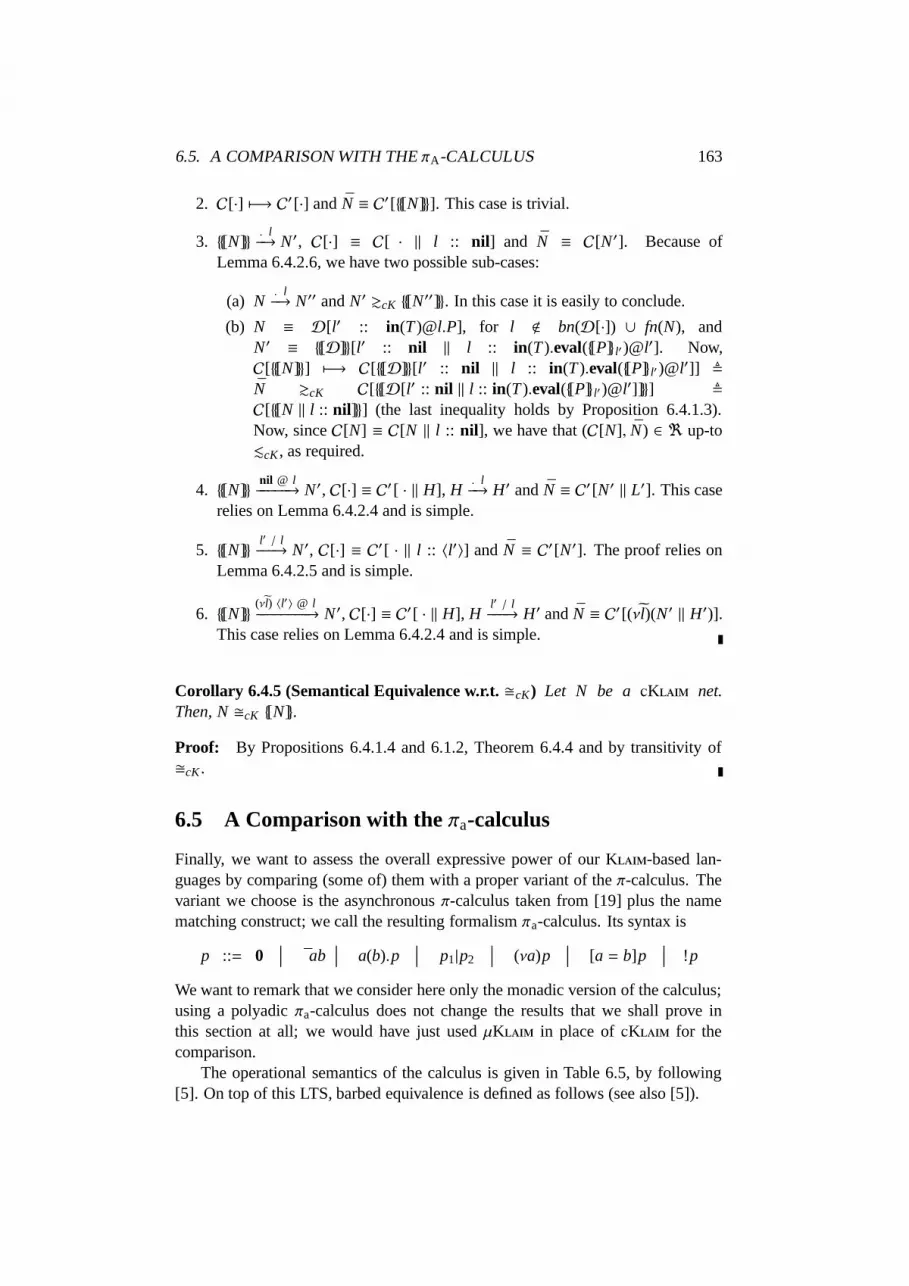
6.5. A COMPARISON WITH THE πA-CALCULUS 163
2. C[·] 7−→ C′ [·] and N ≡ C′[[N]]. This case is trivial.
3. [N]. l−→ N′, C[·] ≡ C[ · ‖ l :: nil] and N ≡ C[N′]. Because of
Lemma 6.4.2.6, we have two possible sub-cases:
(a) N. l−→ N′′ and N′ &cK [N′′]. In this case it is easily to conclude.
(b) N ≡ D[l′ :: in(T )@l.P], for l < bn(D[·]) ∪ fn(N), andN′ ≡ [D][l′ :: nil ‖ l :: in(T ).eval([P]l′ )@l′]. Now,C[[N]] 7−→ C[[D][l′ :: nil ‖ l :: in(T ).eval([P]l′ )@l′]] ,N &cK C[[D[l′ :: nil ‖ l :: in(T ).eval([P]l′ )@l′]]] ,
C[[N ‖ l :: nil]] (the last inequality holds by Proposition 6.4.1.3).Now, since C[N] ≡ C[N ‖ l :: nil], we have that (C[N], N) ∈ < up-to.cK , as required.
4. [N]nil @ l−−−−−→ N′, C[·] ≡ C′ [ · ‖ H], H
. l−→ H′ and N ≡ C′ [N′ ‖ L′]. This case
relies on Lemma 6.4.2.4 and is simple.
5. [N]l′ / l−−−→ N′, C[·] ≡ C′[ · ‖ l :: 〈l′〉] and N ≡ C′[N′]. The proof relies on
Lemma 6.4.2.5 and is simple.
6. [N](νl) 〈l′〉 @ l−−−−−−−−→ N′, C[·] ≡ C′[ · ‖ H], H
l′ / l−−−→ H′ and N ≡ C′[(νl)(N′ ‖ H′)].
This case relies on Lemma 6.4.2.4 and is simple.
Corollary 6.4.5 (Semantical Equivalence w.r.t. cK) Let N be a K net.Then, N cK [N].
Proof: By Propositions 6.4.1.4 and 6.1.2, Theorem 6.4.4 and by transitivity ofcK .
6.5 A Comparison with the πa-calculus
Finally, we want to assess the overall expressive power of our K-based lan-guages by comparing (some of) them with a proper variant of the π-calculus. Thevariant we choose is the asynchronous π-calculus taken from [19] plus the namematching construct; we call the resulting formalism πa-calculus. Its syntax is
p ::= 0∣∣∣ ab
∣∣∣ a(b).p∣∣∣ p1|p2
∣∣∣ (νa)p∣∣∣ [a = b]p
∣∣∣ !p
We want to remark that we consider here only the monadic version of the calculus;using a polyadic πa-calculus does not change the results that we shall prove inthis section at all; we would have just used µK in place of K for thecomparison.
The operational semantics of the calculus is given in Table 6.5, by following[5]. On top of this LTS, barbed equivalence is defined as follows (see also [5]).

164 CHAPTER 6. EXPRESSIVENESS OF THE LANGUAGES
abab−→ 0 a(b).p
ac−→ p[c/b]
pµ−→ p′
[a = a]pµ−→ p′
pµ−→ p′
!pµ−→ !p | p′
pµ−→ p′ b < fn(µ)
(νb)pµ−→ (νb)p′
pab−→ p′ a , b
(νb)pa(b)−→ p′
p =α p′µ−→ q′ =α q
pµ−→ q
pab−→ p′ q
ab−→ q′
p | qτ−→ p′ | q′
(∗)
pa(b)−→ p′ q
ab−→ q′ b < fn(q)
p | qτ−→ (νb)(p′ | q′)
(∗)pµ−→ p′ bn(µ) ∩ fn(q) = ∅
p | qµ−→ p′ | q
(∗)
and the obvious symmetric versions of the rules marked with (∗)
Table 6.5: A LTS for the πa-calculus
Definition 6.5.1 (Asynchronous Barbed Equivalence) Asynchronous barbedequivalence, πa , is the largest symmetric relation between πa-calculus processessuch that p πa q implies that
1. whenever p ↓ a, it holds that q ⇓ a,
where p ↓ a , (∃b . pab−→ ∨ p
a(b)−→ ) and p ⇓ a , (p =⇒↓ a)
2. whenever pτ−→ p′, it holds that q =⇒ q′ and p′ πa q′
3. for all names n and for all πa-calculus process r, it holds that (νn)p πa
(νn)q and p|r πa q|r.
6.5.1 Encoding the πa-calculus in K
We now provide an encoding of the πa-calculus in K; it is given in Table 6.6.Like in the previous section, we need a normalisation function between Knets that makes the encoding prompt. It is defined as follows:
nrmL((νl)N) , nrmL∪l(N)
nrmL(N1 ‖ N2) , nrmL(N1) ‖ nrmL(N2)
nrmL(l :: 〈·〉) , l :: 〈·〉
nrmL(l :: C1 | C2) , nrmL(l :: C1) ‖ nrmL(l :: C2)
nrmL(l :: P) ,
l :: P′ ‖ l′ :: 〈l′′〉 if P = out(l′′)@l′.P′ and l′ ∈ L(νl′) (nrmL∪l′ (l :: P′)) if P = new(l′).P′
l :: P if P , | and no previous case holds

6.5. A COMPARISON WITH THE πA-CALCULUS 165
Top-level Encoding:
[[p]]L , proc :: [[p]] ‖ Πn∈L
n :: nil if fn(p) ⊆ L
and proc is a reserved name
Encoding πa-calculus processes:
[[0]] , nil [[(νa)p]] , new(a).[[p]]
[[ ab]] , out(b)@a.nil [[a(b).p]] , in(!b)@a.[[p]]
[[p1|p2]] , [[p1]] | [[p2]] [[!p]] , rec X.([[p]] | X)
[[[a = b]p]] , new(l).out(a)@l.in(b)@l.[[p]]
Table 6.6: Encoding πa-calculus in K
Essentially, the normalisation replaces all actions new with the net resulting fromthe creation of the new nodes and all actions out over existing localities with thenet containing the datum produced by the action. When a net is the encoding ofa πa-calculus process, the continuation of each action out is nil and function nrmdoes not need to be iterated on it.
For the sake of readability, we write nrmL([[p]]L) as [[[p]]]L. Some simple butcrucial properties of nrmL(·) are given in the following proposition, whose proof issimple.
Proposition 6.5.2 Let P be a K process and p be a πa-calculus process. Then
1. if l , l′ then nrmL((νl′)(l :: P)) = nrmL(l :: new(l′).P)
2. [[[p]]]L ‖ l :: nil &cK [[[p]]]L∪l
3. [[p]]L &lcK [[[p]]]L
We now prove a tight correspondence between πa-calculus processes and theirencodings. We start with a correspondence between the labelled semantics of thetwo calculi and then give their operational correspondence.
Lemma 6.5.3 Let p be a πa-calculus process and fn(p) ⊆ L. Then
1. if pab−→ p′ then [[[p]]]L
〈b〉 @ a=======⇒ [[[p′]]]L
2. if pa(b)−→ p′ then [[[p]]]L
(νb) 〈b〉 @ a==========⇒ [[[p′]]]L∪b
3. if pab−→ p′ then [[[p]]]L
b / a=====⇒ N and [[[p′]]]L∪b ≡ N ‖ b :: nil
4. if [[[p]]]L〈b〉 @ a−−−−−→ N then p
ab−→ p′ and N ≡ [[[p′]]]L
5. if [[[p]]]L(νb) 〈b〉 @ a−−−−−−−−→ N then p
a(b)−→ p′ and [[[p′]]]L∪b ≡ N ‖ b :: nil
6. if [[[p]]]Lb / a−−−→ N then p
ab−→ p′ and [[[p′]]]L∪b .cK N ‖ b :: nil

166 CHAPTER 6. EXPRESSIVENESS OF THE LANGUAGES
Proof: By induction on the length of the inferences.
Lemma 6.5.4 (Operational Correspondence) Let p be a πa-calculus process andfn(p) ⊆ L. Then
1. pτ−→ p′ implies that [[[p]]]L =⇒ [[[p′]]]L
2. [[[p]]]Lτ−→ N implies that p
τ−→ p′ and N &cK [[[p′]]]L
Proof: Both the claims are proved by induction on the inference occurring inthe premise. The first statement is quite simple. We give the base cases for thesecond statement. We want to remark that, thanks to the normalisation procedure,the only possible base case is when using rule (LTS-C). Thus, [[[p]]]L , N1 ‖
N2τ−→ N′1 ‖ N′2 , N, because N1
b / a−−−→ N′1 and N2
〈b〉 @ a−−−−−→ N′2. By definition, it must
be that Ni , [[[pi]]]L, for i = 1, 2; moreover, a, b ⊆ fn(N2) ⊆ L. By Lemma 6.5.3.6
and .4, we have that p1ab−→ p′1 and [[[p′1]]]L .cK N′1 ‖ b :: nil, and p2
ab−→ p′2 and
N′2 ≡ [[[p′2]]]L. Thus, p , p1|p2τ−→ p′1|p
′2 , p′. Moreover, N ≡ N′1 ‖ b :: nil ‖
N′2 &cK [[[p′1]]]L ‖ [[[p′2]]]L , [[[p′]]]L, as required.
We now prove that full abstraction can be obtained when considering only thefollowing subset of K contexts, called translated:
C[·] ::= [·]∣∣∣ C[·] ‖ [[p]]L
∣∣∣ (νl)C[·]
Basically, we only permit parallel components resulting from the encoding of πa-calculus processes. This ensures that each free name occurring in any parallelcomponent is also the address of a node in the component itself; this is crucial toprove full abstraction.
Theorem 6.5.5 Let fn(p, q) ⊆ L. Then p πa q if and only if [[[p]]]L trcK [[[q]]]L.
Proof: We start with proving that [[[p]]]L trcK [[[q]]]L implies p πa q. Let < ,
(p , q) : [[[p]]]L trcK [[[q]]]L; we prove that < ⊆ πa . Let p < q. For reduction
closure, we take pτ−→ p′; by Lemma 6.5.4.1 it holds that [[[p]]]L =⇒ [[[p′]]]L. Thus,
[[[q]]]L =⇒ N and [[[p′]]]L trcK N. Then, by using Lemma 6.5.4.2, it can be easily
verified that q =⇒ q′ and [[[q′]]]L .cK N. This suffices to conclude that p′ < q′
since, by the fact that .cK ⊆ cK ⊆ trcK and by transitivity of trcK , it holds that
[[[p′]]]L trcK [[[q′]]]L (notice that, as it is standard in the π-calculus, fn(p′) ⊆ fn(p)
and, thus, fn(p′) ⊆ L – and similarly for q and q′).
We now consider barb preservation; let p ↓ a because pab−→ . By Lemma 6.5.3.1
it holds that [[[p]]]Lb @ a======⇒ ; thus, [[[q]]]L
b @ a======⇒ . Hence, by Lemma 6.5.3.4 and
reduction closure (just proved), it holds that qab==⇒ ; thus, by definition, q ⇓ a. The
case for p ↓ a because pa(b)−→ is similar, but relies on Lemma 6.5.3.2 and .5.
Finally, we have to prove closure under parallel composition and restriction.Let us examine the two conditions separately.

6.5. A COMPARISON WITH THE πA-CALCULUS 167
• We want to prove that (νn)p < (νn)q by knowing that (νn)([[[p]]]L) trcK(νn)([[[q]]]L). By definition, we have that (νn)([[[·]]]L) , [[[(νn) · ]]]L−n andfn((νn) · ) , fn(·) − n. Thus, fn((νn)p, (νn)q) ⊆ L − n and hence[[[(νn)p]]]L−n
trcK [[[(νn)q]]]L−n. By definition of <, this suffices to con-
clude.
• We want to prove that p|r < q|r by knowing that [[[p]]]L ‖ [[[r]]]L′ trcK
[[[q]]]L ‖ [[[r]]]L′ . By definition of [[·]]· and by Proposition 6.5.2.2, itholds that [[[·]]]L ‖ [[[r]]]L′ &cK [[[·]]]L∪L′ ‖ [[[r]]]L∪L′ , [[[ · ‖ r]]]L∪L′ . Thus,[[[p ‖ r]]]L∪L′
trcK [[[q ‖ r]]]L∪L′ and fn(p|r, q|r) = fn(p, q) ∪ fn(r) ⊆ L ∪ L′.
This suffices to conclude.
We are left with proving the converse, i.e. p ≈πa q implies that [[[p]]]L trcK
[[[q]]]L. Let< , ([[[p]]]L , [[[q]]]L) : p ≈πa q; we prove that < is a barbed congru-
ence, up-to .cK . For reduction closure, we let [[[p]]]Lτ−→ N; by Lemma 6.5.4.2
it holds that pτ−→ p′ and N &cK [[[p′]]]L. Then, q =⇒ q′ and p′ πa q′. By
Lemma 6.5.4.1, we know that [[[q]]]L =⇒ [[[q′]]]L; this suffices to conclude up-to .cK .Barb preservation can be proved easily. By Proposition 5.2.3.2 (or .3), [[[p]]]L ↓ a
implies that [[[p]]]L(νb) 〈b〉 @ a−−−−−−−−→ ; by Lemma 6.5.3.4 (or .5) and by definition of barbs
in the πa-calculus, this implies that p ↓ a. Then, q ⇓ a; by using Lemma 6.5.3.1(or .2) and Lemma 6.5.4.1, we obtain the desired [[[q]]]L ⇓ a.
To conclude, we have to prove that, for every translated context C[·], it holdsthat C[[[[p]]]L]< C[[[[q]]]L]. The key observation is that, by definition of translatedcontext, it holds that C[·] ≡ (νn)([·] ‖ [[r]]L′ ). Moreover, by hypothesis, we knowthat (νn)(p|r) πa (νn)(q|r). Hence,
C[[[[·]]]L] ≡ (νn)([[[·]]]L ‖ [[r]]L′ )&cK (νn)([[[·]]]L ‖ [[[r]]]L′ ) by Prop. 6.5.2.3&cK (νn)([[[·]]]L∪L′ ‖ [[[r]]]L∪L′ ) by Prop. 6.5.2.2, (νn)(nrmL∪L′ ([[ · |r]]L∪L′ )), nrmL′′ ((νn)[[ · |r]]L∪L′ ) for L′′ , (L ∪ L′) − n
, nrmL′′ ((νn)(proc :: [[ · |r]] ‖ Πl′∈L∪L′
l′ :: nil))
≡ nrmL′′ ((νn)(proc :: [[ · |r]])) ‖ Πl′∈L′′
l′ :: nil
= nrmL′′ (proc :: [[(νn)( · |r)]]) ‖ Πl′∈L′′
l′ :: nil by Prop. 6.5.2.1
≡ [[[(νn)( · |r)]]]L′′
Notice that, if fn(·) ⊆ L and fn(r) ⊆ L′ (these hold by definition of the encoding),then fn((νn)( · |r)) ⊆ (L ∪ L′) − n , L′′. Thus, C[[[[p]]]L] &cK [[[(νn)(p|r)]]]L′′
< [[[(νn)(q|r)]]]L′′ .cK C[[[[q]]]L]. This suffices to conclude, up-to .cK .
Corollary 6.5.6 (Full Abstraction w.r.t. Translated Barbed Equivalence) Letfn(p, q) ⊆ L. Then p πa q if and only if [[p]]L
trcK [[q]]L.

168 CHAPTER 6. EXPRESSIVENESS OF THE LANGUAGES
Proof: Trivial, by Theorem 6.5.5, Proposition 6.5.2.3 and by observing that .cK ⊆
cK ⊆ trcK .
Remark 6.5.7: On full abstraction w.r.t. barbed equivalence. We have alreadysaid that translated full abstraction seems us the best possible result for the encod-ing of Table 6.6. Indeed, there is a key design issue that breaks full abstraction: inπ-calculus, knowing a name implies that communications can be performed upona channel with that name and these actions succeed whenever a parallel compo-nent performs a complementary action. This is not the case in K (and in thecalculi derived from it). Indeed, it is not necessarily the case that each free nameis associated to a locality (while each name in a π-calculus process is associatedto a channel). This aspect can break full abstraction: e.g., consider the followingπa-calculus equivalence
p , a(x).( x | x.b) πa a(x).( ( x | x.b) ⊕ b ) , q
where ⊕ denotes internal choice. However,
[[p]]L 6cK [[q]]L
Indeed, [[q]]L can produce a datum at node b, while [[p]]L cannot: if the namereceived in the input (that replaces x) is not a node of the net, the encoding of theoutput over x will never produce a datum. Thus, the input from x is blocked andthe following output on b will never produce a datum.
We think that no ‘reasonable’ encoding of πa-calculus in K (nor any othercalculus derived from K) can be given: checking existence of nodes beforefiring an output is a too low-level feature that cannot be implemented in such anabstract setting as the π-calculus. There are two ways in which we can recover fullabstraction.
1. We can make K higher-level: a simple way to do this is to add thefollowing structural rule to those given in Table 2.3
l :: nil ≡ 0
In this way, we recover the π-calculus’ philosophy that each name is alwaysassociated to a communication medium (up-to ≡).
Another possibility is to consider a typed language, where types ensurethat, if a locality name is eventually used as target of an operation, then anode whose address is that name is present in the net. This strongly resem-bles Dπ’s framework [90].
2. We can make the πa-calculus lower-level: some names are channels, whilethe other ones are just communicable objects. This can be formalised bystructuring the syntax of the πa-calculus as follows:
Systems S ::= ∃a∣∣∣ (νa)S
∣∣∣ S 1 | S 2
∣∣∣ pProcesses p ::= . . .

6.5. A COMPARISON WITH THE πA-CALCULUS 169
Encoding Nets:
([0]) , ! ex〈〉 ([N1 ‖ N2]) , ([N1]) | ([N2])
([(νl)N]) , (νl)(([N]) | ! ex l) ([l :: C]) , ([C])l | ! ex l
Encoding Processes:
([nil])u , 0 ([〈l〉])u , u l
([X])u , X ([rec X.P])u , rec X.([P])u
([C1|C2])u , ([C1])u | ([C2])u ([new(l).P])u , (νl)(([P])u | ! ex l)
([out(u′).P])u , u u′ | ([P])u ([in(!x).P])u , u(x).([P])u
([in(u′).P])u , rec X.u(x).(νc)( c | [x = u′]c.([P])u | c.( u x | X)) (∗)
([eval(Q)@u′.P])u , rec X.ex(x).(νc)( c | [x = u′]c.(([P])u | ([Q])u′) | c.X ) (∗)
(∗) for x, X fresh
Table 6.7: Encoding K in πa-calculus
where the particle ∃a implements the presence of a channel with name a.The operational semantics of Table 6.5 must be then modified by followingthe lines of the LTS in Table 3.8 (by adding a check of existence of a channelbefore firing an output action). We call π∃a this lower-level calculus.
6.5.2 Encoding K in the πa-calculus
We now present an encoding of the simplest K-based calculus, namely K-, in the πa-calculus. The encoding is somehow inspired from the encoding ofK in µK (for the handling of names) and of µK in K (for theencoding of the name matching construct of K).
We can follow the correspondence between channels and localities that wepointed out in Section 6.5.1 and translate each locality to a channel. Output actionsperformed at l, as well as data located at l, can be translated to output particlesof the πa-calculus l . Similarly, input actions performed at l can be translated toinput prefixes of the πa-calculus l(x). . Finally, any action new(l′) is translatedto a restriction (νl′). Thus, the correspondence between the two calculi is quitestraightforward up to now.
A first feature that distinguish K from πa-calculus is the communicationparadigm and, mainly, the name matching of K (that happens while retriev-ing a datum). This issue can encoded quite easily, if we accept divergence: processin(l′).P running at l can be translated into a process that first retrieves a datum at land then checks if it is l′; if the check succeeds, the process continues, otherwise itplaces back the accessed datum and looks for another one.
A second feature that distinguish K from πa-calculus is the allocation ofprocesses and their movements, together with the check of locality existence before

170 CHAPTER 6. EXPRESSIVENESS OF THE LANGUAGES
migration. Process distribution is relevant in K to establish where actionsout and in have to take place. Thus, we can define a parameterised encoding forprocesses, ([P])u, where u is the locality where P runs. Then, if P is of the formout(u′).Q, we translate it to uu′ | ([Q])u, while, if P is of the form in(!x).Q, wetranslate it to u(x).([Q])u. A process P of the form eval(Q)@u′.R running at u istranslated to the parallel composition of ([R])u and ([Q])u′ , if existence of locality u′
is ascertained.The last feature we have to model is the distinction between names that are
addresses of network nodes and raw names. The former ones can be then usedas target of remote operations (in the case of K only actions eval), whilethe latter ones cannot. By using a π-calculus terminology, only the first ones areNames (we intentionally used the capital letter), while the latter ones are just val-ues. However, the status of a name (without the capital letter) can change accordingto the context: a Name will always remain such in any context, while a value l canbecome a Name if the context provides a node with address l.
To deal with this sophisticated feature (that, as we have already discussed inRemark 6.5.7, creates a relevant gap between πa-calculus and K-based calculi),we use a reserved channel ex to record existence of localities. Thus, if l is a Namein the K net considered for translation, then channel ex will repeatedly offerl in the encoded net, i.e. the encoding will contain a process of the form
! ex l , (νc)( c l | !c(x)( c x | ex x))
The encoding is reported in Table 6.7. There, we also assume the possibilityof writing πa-calculus processes with recursion – that can be implemented throughreplication, as usual – and we write c and c to mean output and input of dummydata. In the translation of actions in(l) and eval, the fresh restricted channel c isused to implement a form of internal choice. In both cases, the first addendumcan evolve only if the name matching succeeds. On the other hand, the secondaddendum can always be executed: this fact introduces divergence in the encoding.Notice, however, that exactly one of the two addendum can evolve. Finally, like inthe encoding of K in µK, the fact that ex always provides data is necessaryto obtain a fully abstraction result w.r.t. translated contexts. Again, translatedcontexts do not have a full discriminating power over this channel.
The proof of soundness somehow follows proofs already given in the chapter;we only sketch the main steps and leave the details to the interested reader. First,the translated barbed expansion in the πa-calculus, written .tr
πa, can be defined by
following Definition 6.1.1. By following Proposition 6.1.2, it can be proved that.trπa⊂trπa
and, by following Lemma 6.1.5, that translated barbed congruence up-to .tr
πais contained in tr
πa. Then, we can prove that each K reduction is
preserved by its encoding.
Lemma 6.5.8 If N 7−→ N′, then ([N]) =⇒&trπa
([N′]).
Now, since the encoding ([·]) is divergent, we can follow the ideas of Section 6.3and define partial reducts and partial states. Notice that, since divergence can orig-

6.5. A COMPARISON WITH THE πA-CALCULUS 171
inate both from the encoding of name matching and of migrations, we have twopossible cases for partial reducts.
Definition 6.5.9
1. A πa-calculus process p is a partial reduct of a K net N whenever
• N ≡ l :: in(l′).P | 〈l′〉 andp trπa
(νc)( c | [x = l′]c.([P])u | c.(l x | ([in(T ).P])l)) | ! ex l, or
• N ≡ l :: eval(Q)@l′.P ‖ l′ :: nil andp trπa
(νc)( c | [x = l′]c.(([P])l | ([Q])l′ ) | c.([eval(Q)@l′.P])l )| ! ex l | ! ex l′.
2. A πa-calculus process p is a partial state of a K net N whenever N ≡(νl)(N1 ‖ · · · ‖ Nn ‖ N), p ≡π (νl)(p1 ‖ · · · ‖ pn ‖ ([N])) and for all i it holdsthat pi is a partial reduct of Ni (where ≡π is Milner’s structural equivalence,see [112]).
The pleasant property of µK’s partial reducts is here stronger.
Lemma 6.5.10 Let p be a partial reduct of N. Then,
• N ≡ l :: in(l′).P | 〈l′〉 and pτ−→ p′ imply that either p′ &tr
πa([N]), or p′ &tr
πa
([P])l | ! ex l.
• N ≡ l :: eval(Q).P ‖ l′ :: nil and pτ−→ p′ imply that either p′ &tr
πa([N]), or
p′ &trπa
([P])l | ([Q])l′ | ! ex l | ! ex l′.
We can now state the reflection of reduction steps.
Lemma 6.5.11 If 〈|N|〉τ−→ p, then either N
τ−→ N′ and p &tr
πa〈|N′|〉, or p is a partial
state of N.
Finally, it is easy to see that the encoding faithfully translates the barbs; it onlyadds new barbs on ex but no translated context can fully observe them. Hence, theproof of the following concluding theorem can be carried on easily.
Theorem 6.5.12 (Full Abstraction w.r.t. Translated Barbed Congruence)N lcK M if and only if ([N]) tr
πa([M]).
Proof: For the ‘if’ direction, it suffices to prove that relation
< , (N,M) : ([N]) trπa
([M])∪ (N,M) : ∃ p. ([N]) trπa
p ∧ p partial state of M∪ (N,M) : ∃ p. 〈|M|〉 trπa
p ∧ p partial state of N

172 CHAPTER 6. EXPRESSIVENESS OF THE LANGUAGES
is barb preserving, reduction closed (up-to .lcK) and closed under translated con-texts (again, up-to .lcK). For the ‘only if’ direction, it suffices to prove that relation
< ,⋃
N lcK M ( ([N]), ([M]) )∪ ( ([N]), p) : p partial state of M∪ (p, ([M])) : p partial state of N
is barb preserving, reduction closed (up-to .trπa
) and closed under translated con-texts (again, up-to .tr
πa).
6.6 Concluding Assessment and Related Work
The main results of this chapter are summarised in Table 6.8. There, a labelled
arrow between two calculi, XP−→ Y, means that the language X can be encoded in
the language Y and the encoding enjoys property P. The arrow is dotted if theencoding can introduce divergence, i.e. infinite sequences of reductions that in thesource term were not present.
According to Palamidessi [122], each ‘reasonable’ encoding enc(·) should en-joy at the very least the following properties:
1. homomorphic w.r.t. the parallel operator, i.e. enc(N ‖ M) = enc(N) ‖enc(M) (this is needed in order to maintain the degree of parallelism duringthe translation);
2. preserving renaming, i.e. for every permutation of names σ in the sourcelanguage there exists a permutation of names θ in the target language suchthat enc(Pσ) = (enc(P))θ (this ensures that the translation does not dependon the names involved);
3. preserving the basic observables, i.e. it has to preserve the visible behavioursof the encoded terms;
4. preserving termination, i.e. it has to turn each terminating term in a termi-nating term.
All the encodings we have presented in this chapter enjoy properties 2. and 3. .About property 4., it is not enjoyed by the encodings of µK in K and ofK into the πa-calculus. This is related to the fact that, in our opinion, theform of name matching present in the K-based calculi (that, in turn, has beeninherited by L [74]) is very powerful: it allows to perform boolean tests onnames while retrieving them. A similar feature led to the separation result of [122]between the synchronous and the asynchronous π-calculus. About property 1., itis not enjoyed by the encoding of the πa-calculus in K (where, however, wehave [[N ‖ M]] ≡ [[N]] ‖ [[M]]) and by the encoding of K in µK. In this casewe have a centralised entity (the locality env) that coordinates the translation of

6.6. CONCLUDING ASSESSMENT AND RELATED WORK 173
KLAIM µKLAIM CKLAIM
πa-calculus
L-CKLAIM
F. A. w.r.t. ≅tr
F. A. w.r.t. ≅tr
S. E. w.r.t. ≅
F. A. w.r.t. ≅tr
F. A. w.r.t. ≅tr
where: F.A. stands for Fully Abstract,S .E. stands for Semantically Equivalent,→ stands for the identity encoding,d stands for a divergent encoding,−→ stands for a divergence-free encoding.
Table 6.8: Overview of our Results
names. According to Nestmann [118], the presence of such centralised authoritiesnot necessarily implies that the encoding developed is weak: in practice, indeed,the resolution of names in Internet (through the so called DNS) requires some formof centralised knowledge to turn logical names in IP addresses. Hence, we believethat in this framework, property 1. is not strictly necessary.
Concluding assessment. We can now define a hierarchy of the properties en-joyed by our encodings. This can be done by relying on the properties pointed outin [122] and by the facts that tr is coarser than and that semantical equivalenceimplies fully abstraction (w.r.t. the same equivalence). If we let ‘’ mean ‘betterthan’, we have that
S .E. w.r.t. −−−−−−−−−→
F.A. w.r.t. tr
−−−−−−−−−→ F.A. w.r.t. tr
− − − − − →
174 CHAPTER 6. EXPRESSIVENESS OF THE LANGUAGES
Thus, the encoding of K in K is the best we can imagine: it doesnot introduce divergence and it turns a source net in a barbed congruent target net.The fact that barbed congruence is a fine-grained equivalence makes our result evenstronger. Hence, the two calculi have exactly the same expressive power; the useof remote communications is only to ease programming.
The encoding of K in µK and of πa-calculus in K are still goodresults. Hence, the source and the target languages have comparable expressivepower. Moreover, the complexity of the code generated by the encoding procedureis quite limited, especially in the second encoding.
The weaker results are the encodability of µK in K and of Kin πa-calculus; this is not surprising since, as we already said, this is related tothe expressive form of name matching we used. A part from divergence, we alsohave that the encoding of polyadic communication of µK into monadic oneof K is not simple and efficient. Table 6.2 substantiates this claim: a lotof monadic exchanges are necessary to implement each polyadic communication.While this could be acceptable from a theoretical point of view, it is hardly usablein practice. To conclude, we believe that, in a L-like framework, these twoforms of communication are not freely interchangeable. Hence, µK is rathermore expressive than K.
Clearly, the results in this paper do not prove that µK and K aremore powerful than K and πa-calculus, respectively. To this aim, we shouldpresent some impossibility results similar to that in [122]. We are now working onproving an impossibility result for an encoding of K in the πa-calculus; webelieve that, due to the check of existence of the target of a communication (thatis performed in K and not in πa-calculus), this result should hold. Aboutthe encodability of a polyadic communication through monadic communications(µK into K), we think that a divergence-free encoding should not exist.Indeed, the fields of a polyadic datum can only be accessed one by one; in thisway, we are forced to split the atomic activity of function match into a field-by-field compliance checking. Such checking must be suspended whenever the datumaccessed does not match with the template used to retrieve it, and the inputtingprocess must be rolled back, to let it try to access another datum. Then, the pos-sibility of repeatedly accessing the same (non-matching) datum clearly leads todivergence. Again, this is not a formal argument but we find it quite convincing.
Finally, as we have already said, tr is enough to state expressiveness results.On the other hand, an encoding can be also considered as a formal descriptionof how a language primitive can be implemented by means of other primitives;then, the complexity of the encoding can be used as a measure of the power ofthe primitive. We plan to investigate this aspect in a future work. However, wecan already say that tr will be too weak in such setting: preorders based on somenotion of cost (maybe relying on whether an action is remote or not) should beused instead.

6.6. CONCLUDING ASSESSMENT AND RELATED WORK 175
Related work. The works on encodings of process calculi that are strictly relatedto our approach have been discussed throughout the chapter. We want to concludeby examining the impact on expressiveness of alternative operators that have con-sidered when designing K.
In [29] three different semantics for the output operation are studied in thesetting of a simple Linda-based process calculus: instantaneous output (an outputprefix immediately unleashes the corresponding tuple in the TS), ordered output(a reduction is needed to turn an output prefix into the corresponding tuple in theTS) and unordered output (two reductions are needed to turn an output into anavailable tuple, i.e. one to send the tuple to the TS and another one to make thetuple available in the TS). According to this terminology, the semantics of Koutput operation is ordered.
In [29] it is proved that the instantaneous semantics yields the most expressivesetting. We believe that the instantaneous semantics would simplify the theory de-veloped in this paper. For example, the proofs for the encoding of the πa-calculusinto Kwould be simpler: the encoding would be prompt and no normalizationwould be needed. However, instantaneous tuple emission is unrealistic, especiallyin a global computing scenario where remote operations are enabled. On the otherhand, unordered outputs are very close to the practice of global computers (con-sider, e.g., sending e-mail messages). We believe that the theory presented in thispaper can be tailored to deal with such semantics. However, in [30] it is proved thatthe simple Linda-based process calculus considered in [29] is Turing powerful un-der the instantaneous and ordered semantics but not with the unordered semantics.The output operation of K represents a compromise between expressivenessand implementability.
The calculi considered in this paper do not have a general non-deterministicchoice operator. This composition mechanism of ‘classical’ process calculi (e.g.CCS, CSP, ACP, π-calculus) is useful for specifying systems but is hardly imple-mentable (this is especially true in distributed environments), thus it is missing inmany languages designed while taking implementation issues into account. Forexample, the πa-calculus is often presented without nondeterministic choice. Froma theoretical point of view, one may wonder if the addition of (restricted forms of)the non-deterministic choice operator to the considered calculi would change theirexpressive power.
Since the same issue has been deeply studied in the setting of the πa-calculus,let us first briefly summarize some relevant results. [119] presents two encodingsof the πa-calculus with input-guarded choice (where each summand begins withan input action) into ‘pure’ πa-calculus, and [118] defines an encoding of a variantof the π-calculus with separate choice (where all summands begin with the samekind of action) in the πa-calculus. [122] shows that no ‘reasonable’ encoding ofthe π-calculus with mixed choice (where each summand begins with an action)in the πa-calculus can be ever given. Since synchronous communication can beencoded through asynchronous communication, [93, 19, 31], it follows that, in thesetting of the πa-calculus, the introduction of (some forms of) non-deterministic

176 CHAPTER 6. EXPRESSIVENESS OF THE LANGUAGES
choice changes the expressive power of the language. Similar conclusions can bedrawn for the K-based languages we considered. By following [119, 118],we could implement restricted non-deterministic choice. However, we have to saythat a restricted form of choice is provided implicitly by K and all its variantsthrough actions read/in actions: their semantics is determined by the availabilityof tuples matching a given template, and in case of multiple matching the choice isinternally determined.

Chapter 7
Conclusion and Future Work
This thesis collects some foundational work on calculi based on the paradigm putforward by the language K. To sum up, the main contributions contained inthis thesis are:
• the definition of a family of foundational calculi based on K,
• the presentation of type systems for security driven by global computingrequirements,
• the development of non-trivial, but still tractable, notions of behaviouralequivalences,
• the assessment of the calculi presented from the point of view of their ex-pressiveness.
The strength and the usefulness of these efforts should be witnessed by the exam-ples provided throughout the thesis. In particular, we took into account severalscenarios, ranging from e-commerce to on-line banking, from multiuser systems todistributed protocols. Moreover, the encodings used to carry on the analysis of theexpressive power of the calculi should also have improved the understanding of theK and the appreciation of its specific design choices, that make it significantlydifferent from the standard process calculi and from the other calculi for GC.
Further developments. While writing this thesis, we extended the work onK-derived calculi with several issues like dynamic inter-node connections [60],failures [63] and more flexible forms of pattern-matching [64]. We did not includehere such results to save space. However, it is worth saying that the work we havejust presented was the basis for all these enhancements. This fact furtherly sub-stantiates the claim that this thesis acts as a crucial foundational work within theK project.
177

178 CHAPTER 7. CONCLUSION AND FUTURE WORK
Future work. In addition to the work covered by this thesis, we studied otherpossible approaches to security in calculi with mobility, that could be integratedwith the work presented here. We now conclude by discussing the most interestingissues.
In Chapter 3, we expressed node policies in a very simple way, essentially assets of process actions. More sophisticated possibilities are available. For example,we could exploit the theory developed in [23], where we study the impact of r ole-based access control (RBAC, [132]) mechanisms within a distributed π-calculus.The policies we used in this paper can be defined in a more flexible way by usingthe RBAC approach. Moreover, in [78] we work on a very simple distributed calcu-lus with code mobility where several fine-grained policies are expressed by using,e.g., finite automata. By properly modifying the types presented in Chapter 3, webelieve that the theory developed in loc.cit. can be adapted to the K setting.
A concrete issue that we totally ignored in this thesis is the use of cryptogra-phy. As we have already remarked several times, cryptography is a fundamentallower-level tool to ensure that GCs work properly. Thus, in [17, 18], we workedon the Spi-calculus [1], a cryptographic version of the π-calculus, to develop asound and complete axiomatisation for finite processes under a bisimulation-basedsemantics; then, we used some equational laws to show the correctness of the pro-tocol K. Clearly, cryptography is an orthogonal issue with respect to thetopics covered by this thesis. A challenging direction for future research is to studythe integration of cryptographic primitives in a calculus with mobile agents, likeK.

Appendix A
Symbols and Notations
In Chapter 2:L : locality names (in K)V : locality variables (in K)N : names (in µK, K and K)ρ : allocation environments (finite mappings of names for variables)
fn(·), bn(·) : free and bound namesfv(·), bv(·) : free and bound variables (in K)E[[ · ]]ρ : the evaluation function of a tuple/template w.r.t. ρmatch : the pattern-matching function (between a template and a tuple)σ : . substitutions of names and processes for variables in K
. substitutions of names for names in µK, K andK
ε : the empty substitution : the composition of substitutions≡ : the structural congruence relation7−→ : the reduction relation
In Chapter 3:C : the set of process capabilitiesπ : sets of capabilitiesΠ : the powerset of C (i.e., the set of all the πs)vΠ
: an ordering on Πd : the pointwise union of functionsΓ : typing environments
upd : the extension of a type environment with the typing annotationsfor the names bound in a template
: the run-time error predicate
179

180 APPENDIX A. SYMBOLS AND NOTATIONS
In Sections 3.2 and 3.3:δ : types and type environments : the subtyping relation
matchδ : the typed pattern-matching function
In Section 3.4:p : a finite set of template patternsP : the set of all template patterns
T (·) : the set of all templates complying with a set of patterns∆ : types⊥ : the empty type6 : the subtyping relation
match∆(l) : the typed pattern-matching function
In Chapter 4:r : regions (i.e., finite subsets of L)> : all the net (i.e., the largest region)R : the set of all regions : the type annotation procedure] : the union of functions with disjoint domains+ : the extension of information in a typing environment
reg(·) : a function returning the intersection of regions in ·S : turning each region r in > within a typing environment ,
if r ∩ S , ∅ : tagged typing annotation
7−→→ : tagged reduction relation
In Chapter 5:↓, ⇓ : strong and weak basic observable (or barb)C[·] : net context : reduction barbed congruence' : may testing≈ : (labelled) bisimulation
−→ , =⇒ : strong and weak labelled transitionsτ : silent actionI : inert node componentsα : labels for the bisimulation : trace equivalenceµ : labels for the trace equivalence% : traces (i.e., sequences of visible actions)ε : empty trace· : concatenation of traces : ordering relation on traces· : complementation on traces
q(%) : canonical observer for trace %

181
In Chapter 6:. : expansion preorder
tr : translated reduction barbed congruence.tr : translated expansion preorder〈(·)〉 : encoding K in µK〈〈(·)〉〉 : normalisation of 〈(·)〉〈|·|〉 : encoding µK in K[·] : encoding K in K[·] : normalisation of 〈(·)〉[[·]] : encoding πa-calculus in K
[[[·]]] : normalisation of [[·]]([·]) : encoding K in πa-calculus

182 APPENDIX A. SYMBOLS AND NOTATIONS

Bibliography
[1] M. Abadi and A. D. Gordon. A calculus for cryptographic protocols: The Spicalculus. Information and Computation, 148(1):1–70, 1999. An extended abstractappeared in the Proc. of the 4th ACM Conf. on Computer and CommunicationsSecurity, 1997.
[2] A. Acharya, M. Ranganathan, and J. Saltz. Sumatra: A Language for Resource-aware Mobile Programs. In J. Vitek and C. Tschudin, editors, Mobile Object Sys-tems: Towards the Programmable Internet, volume 1222 of LNCS, pages 111–130.Springer, 1997.
[3] G. Agha. A Model of Concurrent Computation in Distributed Systems. MIT Press,1986.
[4] R. Amadio. On modelling mobility. Theoretical Computer Science, 240(1):147–176, 2000.
[5] R. M. Amadio, I. Castellani, and D. Sangiorgi. On bisimulations for the asyn-chronous π-calculus. Theoretical Computer Science, 195(2):291–324, 1998. Anextended abstract appeared in Proc. of CONCUR ’96, LNCS 1119: 147–162.
[6] K. Arnold, E. Freeman, and S. Hupfer. JavaSpaces Principles, Patterns and Prac-tice. Addison-Wesley, 1999.
[7] K. Arnold and J. Gosling. The Java Programming Language. Addison-Wesley,1996.
[8] H. P. Barendregt. The Lambda Calculus, volume 103 of Studies in Logic and theFoundations of Mathematics. North Holland, 1984 (revised edition).
[9] L. Bettini. Linguistic Constructs for Object-Oriented Mobile Code Programmingand their Implementations. PhD thesis, Dip. di Matematica, Univ. di Siena, 2003.
[10] L. Bettini, V. Bono, R. De Nicola, G. Ferrari, D. Gorla, M. Loreti, E. Moggi,R. Pugliese, E. Tuosto, and B. Venneri. The KLAIM project: Theory and practice.In C. Priami, editor, Global Computing: Programming Environments, Languages,Security and Analysis of Systems, number 2874 in LNCS, pages 88–150. Springer,2003.
[11] L. Bettini, R. De Nicola, G. Ferrari, and R. Pugliese. Interactive Mobile Agentsin X-K. In P. Ciancarini and R. Tolksdorf, editors, Proc. of the 7th IEEEWorkshops on Enablings Technologies: Infrastructure for Collaborative Enterprises(WETICE), pages 110–115. IEEE Computer Society, 1998.
[12] L. Bettini, R. De Nicola, and R. Pugliese. Klava: a Java Package for Mobile Code.Software — Practice and Experience, 32:1365–1394, 2002.
183

184 BIBLIOGRAPHY
[13] M. Boreale. On the expressiveness of internal mobility in name-passing calculi.Theoretical Comput. Sci., 195(2):205–226, 1998. An extended abstract appeared inProceedings of CONCUR ’96, LNCS 1119: 163–178.
[14] M. Boreale and R. De Nicola. Testing equivalences for mobile processes. Informa-tion and Conputation, 120:279–303, 1995. An extended abstract appeared in Proc.of CONCUR ’92, LNCS 630.
[15] M. Boreale, R. De Nicola, and R. Pugliese. Basic observables for processes. Infor-mation and Conputation, 149(1):77–98, 1999.
[16] M. Boreale, R. De Nicola, and R. Pugliese. Trace and testing equivalence on asyn-chronous processes. Information and Computation, 172:139–164, 2002.
[17] M. Boreale and D. Gorla. On compositional reasoning in the spi-calculus. InM. Nielsen and U. Engberg, editors, Proceedings of FoSSaCS ’02, volume 2303of LNCS, pages 67–81. Springer-Verlag, 2002.
[18] M. Boreale and D. Gorla. Process calculi and the verification of security proper-ties. Journal of Telecommunication and Information Technology— Special Issue onCryptographic Protocol Verification, (4):28–40, 2002.
[19] G. Boudol. Asynchrony and the π-calculus (note). Rapport de Recherche 1702,INRIA Sophia-Antipolis, 1992.
[20] G. Boudol. Typing the use of resources in a concurrent calculus. In R. K. Shya-masundar and K. Ueda, editors, Proceedings of ASIAN ’97, volume 1345 of LNCS,pages 239–253. Springer, 1997.
[21] G. Boudol, I. Castellani, F. Germain, and M. Lacoste. Models of distribution andmobility: state of the art. MIKADO Global Computing Project, IST-2001-32222.Deliverable D1.1.1, reference RR/WP1/1. 2002.
[22] G. Boudol, I. Castellani, M. Hennessy, and A. Kiehn. A theory of processes withlocalities. Formal Aspects of Computing, 6:165–200, 1994.
[23] C. Braghin, D. Gorla, and V. Sassone. A distributed calculus for role-based accesscontrol. In Proceedings of 17th CSFW. IEEE Computer Society, 2004. Full versionas Tech. Rep. 08/2004, Dip. di Informatica, Univ. di Roma “La Sapienza”.
[24] M. Bugliesi and G. Castagna. Secure safe ambients. In Proceedings of POPL ’01.ACM, 2001.
[25] M. Bugliesi, G. Castagna, and S. Crafa. Boxed ambients. In Proceedings of TACS’01, number 2215 in LNCS, pages 38–63. Springer, 2001.
[26] M. Bugliesi, G. Castagna, and S. Crafa. Reasoning about security in mobile am-bients. In Proceedings of CONCUR ’01, number 2154 in LNCS, pages 102–120.Springer, 2001.
[27] M. Bugliesi, D. Colazzo, and S. Crafa. Types for discretionary access control. InProceedings of CONCUR’04, number 3170 in LNCS, pages 225–239. Springer,2004.
[28] M. Bugliesi, S. Crafa, M. Merro, and V. Sassone. Communication interferencein mobile boxed ambients. In M. Agrawal and A. Seth, editors, Proceedings ofFSTTCS’02, volume 2556 of LNCS, pages 71–84. Springer, 2002.

BIBLIOGRAPHY 185
[29] N. Busi, R. Gorrieri, and G. Zavattaro. Comparing three semantics for linda-likelanguages. Theoretical Computer Science, 240(1):49–90, 2000.
[30] N. Busi, R. Gorrieri, and G. Zavattaro. On the expressiveness of linda coordinationprimitives. Information and Computation, 156(1-2):90–121, 2000.
[31] D. Cacciagrano and F. Corradini. On synchronous and asynchronous communi-cation paradigms. In Proc. of ICTCS’01, number 2202 in LNCS, pages 256–268.Springer, 2001.
[32] L. Caires and L. Cardelli. A Spatial Logic for Concurrency. Information and Com-putation, 186(2):194–235, 2003. Earlier, this work appeared split in two parts,respectively in Proc. of TACS’01, LNCS 2215, and Proc. of CONCUR’02, LNCS2421.
[33] L. Cardelli. A language with distributed scope. Computing Systems, 8(1):27–59,1995.
[34] L. Cardelli. Abstractions for mobile computation. In J. Vitek and C. Jensen, editors,Secure Internet Programming: Security Issues for Mobile and Distributed Objects,number 1603 in LNCS, pages 51–94. Springer, 1999.
[35] L. Cardelli, G. Ghelli, , and A. D. Gordon. Secrecy and group creation. In Proc. ofCONCUR’00, number 1877, pages 365–379. Springer, 2000.
[36] L. Cardelli, G. Ghelli, and A. D. Gordon. Mobility types for mobile ambients.In J. Wiederman, P. van Emde Boas, and M. Nielsen, editors, Proc. of ICALP’99,volume 1644 of LNCS, pages 230–239. Springer, 1999.
[37] L. Cardelli, G. Ghelli, and A. D. Gordon. Ambient groups and mobility types. InJ. van Leeuwen, O. Watanabe, M. Hagiya, P. Mosses, and T. Ito, editors, Proc. ofIFIP-TCS’00, volume 1872 of LNCS, pages 333–347. Springer, 2000.
[38] L. Cardelli, G. Ghelli, and A. D. Gordon. Types for the ambient calculus. Informa-tion and Computation, 177(2):160–194, 2002.
[39] L. Cardelli and A. D. Gordon. Types for mobile ambients. In Proc. of POPL’99,pages 79–92. ACM, 1999.
[40] L. Cardelli and A. D. Gordon. Anytime, Anywhere: Modal Logics for MobileAmbients. In Proc. of POPL’00. ACM, 2000.
[41] L. Cardelli and A. D. Gordon. Mobile ambients. Theoretical Comput. Sci.,240(1):177–213, 2000. An extended abstract appeared in Proc. of FoSSaCS ’98,number 1378 of LNCS, pages 140-155.
[42] L. Cardelli and A. D. Gordon. Logical Properties of Name Restriction. In S. Abram-sky, editor, Proc. of TLCA’01, number 2044 in LNCS. Springer, 2001.
[43] G. Castagna, G. Ghelli, and F. Z. Nardelli. Typing mobility in the seal calculus.In Proceedings of CONCUR ’01, number 2154 in LNCS, pages 82–101. Springer,2001.
[44] G. Castagna and F. Z. Nardelli. The Seal Calculus Revisited: contextual equivalenceand bisimilarity. In M. Agrawal and A. Seth, editors, Proceedings of FSTTCS’02,volume 2556 of LNCS, pages 85–96. Springer, 2002.

186 BIBLIOGRAPHY
[45] G. Castagna and J. Vitek. Seal: A framework for secure mobile computations. InH. Bal, B. Belkhouche, and L. Cardelli, editors, Internet Programming Languages,number 1686 in LNCS, pages 47–77. Springer, 1999.
[46] I. Castellani. Process algebras with localities. In J. Bergstra, A. Ponse, andS. Smolka, editors, Handbook of Process Algebra, pages 945–1045. Elsevier Sci-ence, 2001.
[47] I. Castellani and M. Hennessy. Distributed bisimulations. Journal of the ACM,36:887–911, 1989.
[48] I. Castellani and M. Hennessy. Testing theories for asynchronous languages. InV. Arvind and R. Ramanujam, editors, Proceedings of FSTTCS ’98, volume 1530of LNCS, pages 90–101, 1998.
[49] S. Castellani, P. Ciancarini, and D. Rossi. The ShaPE of ShaDE: a coordinationsystem. Technical Report UBLCS 96-5, Dip. di Scienze dell’Informazione, Univ.di Bologna, Italy, 1996.
[50] P. Ciancarini, R. Tolksdorf, F. Vitali, D. Rossi, and A. Knoche. Coordinating mul-tiagent applications on the WWW: A reference architecture. IEEE Transactions onSoftware Engineering, 24(5):362–366, 1998.
[51] R. Cleaveland. Tableau-based model checking in the propositional µ-calculus. ActaInformatica, 27(8):725–747, 1990.
[52] Concurrency and Mobility Group at Dipartimento di Sistemi e Informatica, Univer-sita di Firenze. K web page. http://music.dsi.unifi.it.
[53] M. Coppo, M. Dezani, E.Giovannetti, and R. Pugliese. Dynamic and Local Typingfor Mobile Ambients. In Proc. of IFIP-TCS’04. Kluwer, 2004.
[54] F. Corradini and R. De Nicola. Locality based semantics for process algebra. ActaInformatica, 34:291–324, 1997.
[55] S. Dal Zilio and A. D. Gordon. Region analysis and a pi-calculus with groups. InProc. of MFCS’00, number 1893, pages 409–424. Springer, 2000.
[56] N. Davies, S. Wade, A. Friday, and G. Blair. L2imbo: a tuple space based platformfor adaptive mobile applications. In Int. Conference on Open Distributed Process-ing/Distributed Platforms (ICODP/ICDP’97), 1997.
[57] R. De Nicola, G. Ferrari, and R. Pugliese. K: a Kernel Language for AgentsInteraction and Mobility. IEEE Transactions on Software Engineering, 24(5):315–330, 1998.
[58] R. De Nicola, G. Ferrari, and R. Pugliese. Programming Access Control: The KlaimExperience. In C. Palamidessi, editor, Proceedings of CONCUR’00, volume 1877of LNCS, pages 48–65. Springer, 2000.
[59] R. De Nicola, G. Ferrari, R. Pugliese, and B. Venneri. Types for Access Control.Theoretical Computer Science, 240(1):215–254, 2000.
[60] R. De Nicola, D. Gorla, and R. Pugliese. Basic observables for a calculus for globalcomputing. Technical report. 07/2004, Dip. di Informatica, Univ. di Roma “LaSapienza”. An extended abstract will appear in Proc. of ICALP’05.

BIBLIOGRAPHY 187
[61] R. De Nicola, D. Gorla, and R. Pugliese. Confining data and processes in globalcomputing applications. Science of Computer Programming. To appear.
[62] R. De Nicola, D. Gorla, and R. Pugliese. On the expressive power of KLAIM-basedcalculi. Proc. of EXPRESS’04, ENTCS, 128(2):117–130, 2004. Full version asTech. Rep. 09/2004, Dip. di Informatica, Univ. di Roma “La Sapienza”; to appearin Theoretical Computer Science.
[63] R. De Nicola, D. Gorla, and R. Pugliese. Global computing in a dynamic networkof tuple spaces. In J. Jacquet and G. Picco, editors, Proc. of 7th International Con-ference on Coordination Models and Languages (COORDINATION 2005), volume3454 of LNCS, pages 157–172. Springer, 2005.
[64] R. De Nicola, D. Gorla, and R. Pugliese. Pattern matching over a dynamic net-work of tuple spaces. In M. Steffen and G. Zavattaro, editors, Proc. of 7th IFIP In-ternational Conference on Formal Methods for Object Oriented-based DistributedSystems (FMOODS 2005), volume 3535 of LNCS, pages 1–14. Springer, 2005.
[65] R. De Nicola and M. Hennessy. Testing equivalence for processes. TheoreticalComputer Science, 34:83–133, 1984.
[66] R. De Nicola and M. Loreti. A Modal Logic for Mobile Agents. ACM Transac-tions on Computational Logic, 2004. An extended abstract appeared in Proc. ofAMAST’00, LNCS 1816.
[67] P. Degano, F. Levi, and C. Bodei. Safe ambients: Control flow analysis and security.In Proc. of ASIAN’00, volume 1961 of LNCS, pages 199–214. Springer, 2000.
[68] D. Deugo. Choosing a Mobile Agent Messaging Model. In Proceedings of ISADS’01, pages 278–286. IEEE Computer Society, 2001.
[69] M. Dezani-Ciancaglini and I. Salvo. Security types for mobile safe ambients. InProceedings of ASIAN’00, volume 1961 of LNCS, pages 215–236. Springer, 2000.
[70] G. M. F. B. Schneider and R. Harper. A language-based approach to security.In Informatics: 10 Years Ahead, 10 Years Back. Conference on the Occasion ofDagstuhl’s 10th Anniversary, volume 2000 of LNCS, page 86. Springer, 1989.
[71] C. Fournet, G. Gonthier, J.-J. Levy, L. Maranget, and D. Remy. A calculus ofmobile agents. In U. Montanari and V. Sassone, editors, Proceedings of CONCUR’96, volume 1119 of LNCS, pages 406–421. Springer, 1996.
[72] C. Fournet and C. Laneve. Bisimulations for the join-calculus. Theoretical Com-puter Science, 266(1-2):569–603, 2001.
[73] A. Fuggetta, G. Picco, and G. Vigna. Understanging code mobility. IEEE Transac-tions on Software Engineering, 24(5):342–361, 1998.
[74] D. Gelernter. Generative communication in linda. ACM Transactions on Program-ming Languages and Systems, 7(1):80–112, 1985.
[75] D. Gelernter. Multiple tuple spaces in Linda. In E. Odijk, M. Rem, and J.-C. Syre,editors, Proceedings of PARLE ’89, volume 366 of LNCS, pages 20–27. Springer-Verlang, 1989.
[76] General Magic, Inc. Odyssey, 1998. http://www.genmagic.com/-
technology/odyssey.html.

188 BIBLIOGRAPHY
[77] J. Godskesen, T. Hildebrandt, and V. Sassone. A calculus of mobile resources. InL. Brim, P. Jancar, M. Kretınsky, and A. Kucera, editors, Proceedings of CON-CUR’02, volume 2421 of LNCS, pages 272–287. Springer, 2002.
[78] D. Gorla, M. Hennessy, and V. Sassone. Security policies as membranes in systemsfor global computing. In J. Rathke, editor, Proc. of 3rd EATCS Workshop on Foun-dations of Global Ubiquitous Computing (FGUC’04), ENTCS. Elsevier, 2004. Fullversion as Research Rep. 02/2004, Dep. Informatics, Univ. of Sussex; to appear inLogical Methods in Computer Science.
[79] D. Gorla and R. Pugliese. Enforcing security policies via types. In D. Hutter,G. Mueller, W.Stephan, and M. Ullman, editors, Proc. of 1st Intern.Conf. on Se-curity in Pervasive Computing (SPC’03), volume 2802 of LNCS, pages 88–103.Springer-Verlag, 2003. Full version as Tech. Rep. 05/2004, Dip. di Informatica,Univ. di Roma “La Sapienza”.
[80] D. Gorla and R. Pugliese. Resource access and mobility control with dynamic priv-ileges acquisition. In J. Baeten, J. Lenstra, J. Parrow, and G. Woeginger, editors,Proceedings of ICALP’03, volume 2719 of LNCS, pages 119–132. Springer-Verlag,2003. Full version as Tech. Rep. 06/2004, Dip. di Informatica, Univ. di Roma “LaSapienza”.
[81] D. Gorla and R. Pugliese. Controlling data movement in global computing ap-plications. In Proc. of the 19th ACM-SIGAPP Symposium on Applied Computing(SAC’04), pages 1462–1467. ACM, 2004.
[82] R. S. Gray. Agent Tcl: A flexible and secure mobile-agent system. PhD Thesis.Technical Report PCS-TR98-327, Dartmouth College, Computer Science, Hanover,NH, 1997.
[83] R. R. Hansen, J. G. Jensen, F. Nielson, and H. R. Nielson. Abstract interpretationof mobile ambients. In Proc. of SAS’99, number 1694 in LNCS, pages 134–148.Springer, 1999.
[84] M. Hennessy. The security pi-calculus and non-interference. In Proc. of MFPS XIX,ENTCS, 2003. Full version to appear in Journal of Logic and Algebraic Program-ming.
[85] M. Hennessy, M. Merro, and J. Rathke. Towards a behavioural theory of access andmobility control in distributed systems. In Proceedings of FoSSaCS ’03, volume2620 of LNCS, pages 282–299. Springer, 2003. Full version as COGS ComputerScience Technical Report, 2002:01.
[86] M. Hennessy and R. Milner. Algebraic Laws for Nondeterminism and Concurrency.Journal of the ACM, 32(1):137–161, 1985.
[87] M. Hennessy, J. Rathke, and N. Yoshida. SafeDpi: a language for controlling mo-bile code. In Proceedings of FoSSaCS’04, volume 2987 of LNCS, pages 241–256.Springer, 2004.
[88] M. Hennessy and J. Riely. Type-safe execution of mobile agents in anonymousnetworks. In J. Vitek and C. Tschudin, editors, Mobile Object Systems: Towards theProgrammable Internet, volume 1222 of LNCS, pages 111–130. Springer, 1997.

BIBLIOGRAPHY 189
[89] M. Hennessy and J. Riely. Information flow vs. resource access in the asynchronouspi-calculus. In U. Montanari, J. Rolim, and E. Welzl, editors, Proceedings ofICALP’00, volume 1853 of LNCS, pages 415–427. Springer, 2000. Full versionto appear in ACM TOPLAS.
[90] M. Hennessy and J. Riely. Resource Access Control in Systems of Mobile Agents.Information and Computation, 173:82–120, 2002.
[91] C. Hoare. Communicating sequential processes. In R. McKeag and A. Macnaghten,editors, On the construction of programs – an advanced course, pages 229–254.Cambridge university press, 1980.
[92] K. Honda. Types for dyadic interaction. In E. Best, editor, Proceedings of CONCUR’93, volume 715 of LNCS, pages 509–523. Springer, 1993.
[93] K. Honda and M. Tokoro. An object calculus for asynchronous communication.In P. America, editor, Proceedings of ECOOP ’91, volume 512 of LNCS, pages133–147. Springer, 1991.
[94] K. Honda, V. Vasconcelos, and N. Yoshida. Secure information flow as typed pro-cess behaviour. In G. Smolka, editor, Proceedings of ESOP ’00, volume 1782 ofLNCS, pages 180–199. Springer, 2000.
[95] K. Honda, V. T. Vasconcelos, and M. Kubo. Language primitives and type dis-cipline for structured communication-based programming. In C. Hankin, editor,Proceedings of ESOP ’98, volume 1381 of LNCS, pages 122–138. Springer, 1998.
[96] K. Honda and N. Yoshida. On reduction-based process semantics. TheoreticalComputer Science, 152(2):437–486, 1995. An extract appeared in Proc. of FSTTCS’93, LNCS 761.
[97] D. Johansen, F. Schneider, and R. Renesse. What TACOMA Taught Us. In D. Milo-jicic, F. Douglis, and R. Wheeler, editors, Mobility, Mobile Agents and Process Mi-gration - An edited Collection. Addison-Wesley, 1998.
[98] D. Kirli. Confined mobile functions. In Proceedings of 14th CSFW. IEEE ComputerSociety, 2001.
[99] N. Kobayashi. A partially deadlock-free typed process calculus. ACM Transac-tion on Programming Languages and Systems, 20(2):436–482, 1998. An extendedabstract previously appeared in the Proc. of LICS ’97, pages 128–139.
[100] N. Kobayashi. Type systems for concurrent processes: From deadlock-freedom tolivelock-freedom, time-boundedness. In J. van Leeuwen, O. Watanabe, M. Hagiya,P. Mosses, and T. Ito, editors, Proceedings of IFIP TCS 2000, volume 1872 of LNCS,pages 365–389. Springer, 2000.
[101] N. Kobayashi, B. C. Pierce, and D. N. Turner. Linearity and the pi-calculus. InProceedings of POPL ’96, pages 358–371. ACM, 1996.
[102] N. Kobayashi, S. Saito, and E. Sumii. An implicitly-typed deadlock-free processcalculus. In C. Palamidessi, editor, Proceedings of CONCUR ’00, volume 1877 ofLNCS, pages 489–503. Springer, 2000.
[103] D. Lange and M. Oshima. Programming and Deploying Java mobile Agnets withAglets. Addison-Wesley, 1998.

190 BIBLIOGRAPHY
[104] F. Levi and S. Maffeis. An abstract interpretation framework for analysing mobileambients. In Proc. of SAS’01, number 2126 in LNCS, pages 395–411. Springer,2001.
[105] F. Levi and D. Sangiorgi. Controlling interference in ambients. In Proceedings ofPOPL ’00, pages 352–364. ACM, 2000.
[106] M. Loreti. Languages and Logics for Network Aware Programming. PhD thesis,Universita di Siena, 2002. Available at http://music.dsi.unifi.it.
[107] M. Merro and M. Hennessy. Bisimulation congruences in Safe Ambients. In Pro-ceedings of POPL ’02. ACM, 2002.
[108] M. Merro and F. Z. Nardelli. Bisimulation proof methods for mobile ambients.In J. Baeten, J. Lenstra, J. Parrow, and G. Woeginger, editors, Proceedings ofICALP’03, volume 2719 of LNCS. Springer, 2003.
[109] R. Milner. Calculi for synchrony and asynchrony. Theoretical Computer Science,25:267–310, 1983.
[110] R. Milner. Communication and Concurrency. Prentice Hall, 1989.
[111] R. Milner. Sorts in the π-calculus (extended abstract). In E. Best and G. Rozenberg,editors, Proc. of the 3rd Workshop on Concurrency and Compositionality, volume191 of GMD-Studien. GMD Bonn, St. Augustin, 1991.
[112] R. Milner. The polyadic π-calculus: A tutorial. In F. Bauer, W. Brauer, andH. Schwichtenberg, editors, Logic and Algebra of Specification, volume 94 of SeriesF: Computer and System Sciences. NATO Advanced Study Institute, 1993.
[113] R. Milner, J. Parrow, and D. Walker. A Calculus of Mobile Processes, I and II.Information and Computation, 100(1):1–40, 41–77, 1992.
[114] R. Milner, J. Parrow, and D. Walker. Modal logics for mobile processes. TheoreticalComputer Science, 114:149–171, 1993.
[115] R. Milner and D. Sangiorgi. Barbed bisimulation. In W. Kuich, editor, Proceedingsof ICALP ’92, volume 623 of LNCS, pages 685–695. Springer, 1992.
[116] U. Montanari and M. Pistore. Finite state verification for the asynchronous pi-calculus. In R. Cleaveland, editor, Proc. of TACAS’99, volume 1579 of LNCS,pages 255–269. Springer, 1999.
[117] G. Necula. Proof-carrying code. In Proc. of POPL ’97, pages 106–119, 1997.
[118] U. Nestmann. What is a ‘good’ encoding of guarded choice? Information and Com-putation, 156:287–319, 2000. An extended abstract appeared in the Proceedings ofEXPRESS ’97, volume 7 of ENTCS.
[119] U. Nestmann and B. C. Pierce. Decoding choice encodings. Information and Com-putation, 163:1–59, 2000. An extended abstract appeared in the Proceedings ofCONCUR ’96, LNCS 1119, pages 179–194.
[120] F. Nielson, H. R. Nielson, R. R. Hansen, and J. G. Jensen. Validating firewalls inmobile ambients. In J. C. Baeten and S. Mauw, editors, Proceedings of CONCUR’99, volume 1664 of LNCS, pages 463–477. Springer, 1999.
[121] A. Omicini and F. Zambonelli. Coordination for internet application development.Autonomous Agents and Multi-agent Systems, 2(3):251–269, 1999.

BIBLIOGRAPHY 191
[122] C. Palamidessi. Comparing the expressive power of the synchronous and the asyn-chronous π-calculi. Mathematical Structures in Computer Science, 13(5):685–719,2003. An extended abstract appeared in Proc. of POPL’97, ACM Press.
[123] D. Park. Concurrency and automata on infinite sequences. In P. Deussen, editor, 5thGI Conference, volume 104 of LNCS. Springer, 1981.
[124] J. Parrow. An introduction to the pi-calculus. In J. Bergstra, A. Ponse, andS. Smolka, editors, Handbook of Process Algebra, pages 479–543. Elsevier Sci-ence, 2001.
[125] G. Picco, A. Murphy, and G.-C. Roman. L: Linda Meets Mobility. In D. Garlan,editor, Proc. of the 21st Int. Conference on Software Engineering (ICSE’99), pages368–377. ACM, 1999.
[126] B. C. Pierce and D. Sangiorgi. Typing and subtyping for mobile processes. Mathe-matical Structures in Computer Science, 6(5):409–454, 1996. An extract appearedin Proc. of LICS ’93: 376–385.
[127] B. C. Pierce and D. N. Turner. Pict: A programming language based on the pi-calculus. In G. Plotkin, C. Stirling, and M. Tofte, editors, Proof, Language andInteraction: Essays in Honour of Robin Milner. MIT Press, 2000.
[128] J. Riely and M. Hennessy. A typed language for distributed mobile processes. InProceedings of POPL ’98. ACM, 1998.
[129] J. Riely and M. Hennessy. Trust and partial typing in open systems of mobile agents.In Proceedings of POPL ’99, pages 93–104. ACM, 1999. Full version to appear inJournal of Automated Reasoning, 2003.
[130] J. Riely and M. Hennessy. Distributed processes and location failures. TheoreticalComputer Science, 266:693–735, 2001.
[131] A. Rowstron. WCL: A web co-ordination language. World Wide Web Journal,1(3):167–179, 1998.
[132] R. Sandhu, E. Coyne, H. Feinstein, and C. Youman. Role-Based Access ControlModels. IEEE Computer, 29(2):38–47, 1996.
[133] D. Sangiorgi. Expressing Mobility in Process Algebras: First-Order and Higher-Order Paradigms. PhD thesis, 1993. CST-99-93 (also published as ECS-LFCS-93-266).
[134] D. Sangiorgi. Bisimulation in higher-order process calculi. Information and Compu-tation, 131:141–178, 1996. An early version appeared in Proc. of PROCOMET’94,pages 207–224.
[135] D. Sangiorgi. The name discipline of uniform receptiveness. Theoretical ComputerScience, 221(1–2):457–493, 1999. An abstract appeared in the Proc. of ICALP ’97,LNCS 1256, pages 303–313.
[136] D. Sangiorgi. Reasoning about concurrent systems using types. In W. Thomas,editor, Proceedings of FoSSaCS ’99, volume 1578 of LNCS, pages 31–40. Springer,1999.
[137] D. Sangiorgi. Asynchronous process calculi: the first-order and higher-orderparadigms (tutorial). Theoretical Computer Science, 253(2):311–350, 2001.

192 BIBLIOGRAPHY
[138] D. Sangiorgi and D. Walker. The π-calculus: a Theory of Mobile Processes. Cam-bridge University Press, 2001.
[139] P. Sewell. Global/local subtyping and capability inference for a distributed pi-calculus. In K. G. Larsen, S. Skyum, and G. Winskel, editors, Proceedings of ICALP’98, volume 1443 of LNCS, pages 695–706. Springer, 1998.
[140] P. Sewell, P. Wojciechowski, and B. Pierce. Location independence for mobileagents. In H. Bal, B. Belkhouche, and L. Cardelli, editors, Proceedings of ICCL’98, volume 1686 of LNCS. Springer, 1999.
[141] C. Stirling and D. Walker. Local model checking in the modal mu-calculus. Theo-retical Computer Science, 89(1):161–177, 1991.
[142] P. Thati, R. Ziaei, and G. Agha. A Theory of May Testing for Actors. In Proc. ofFMOODS’02, pages 147–162. Kluwer, 2002.
[143] B. Thomsen, L. Leth, and T.-M. Kuo. A Facile tutorial. In U. Montanari andV. Sassone, editors, Proceedings of CONCUR ’96, volume 1119 of LNCS, pages278–298. Springer, 1996.
[144] D. N. Turner. The Polymorphic Pi-Calculus: Theory and Implementation. PhDthesis, 1996. CST-126-96 (also published as ECS-LFCS-96-345).
[145] A. Unyapoth and P. Sewell. Nomadic Pict: Correct communication infrastructuresfor mobile computation. In Proceedings of POPL ’01, pages 116–127. ACM, 2001.
[146] R. van Glabbeek. The linear time - branching time spectrum. In J. Baeten andJ. Klop, editors, Proceedings of CONCUR’90, volume 458 of LNCS, pages 278–297. Springer, 1990.
[147] R. van Glabbeek. The linear time - branching time spectrum II; the semantics of se-quential systems with silent moves. In E. Best, editor, Proceedings of CONCUR’93,volume 715 of LNCS, pages 66–81. Springer, 1993.
[148] J. E. White. Telescript Technology: The Foundation for the Electronic Marketplace.White paper, General Magic, Inc., Mountain View, CA, 1994.
[149] J. E. White. Mobile Agents. In J. Bradshaw, editor, Software Agents. AAAI Pressand MIT Press, 1996.
[150] G. Winskel. A note on model checking the modal ν-calculus. In G. Ausiello,M. Dezani-Ciancaglini, and S. R. D. Rocca, editors, Proc. of the 16th ICALP, vol-ume 372 of LNCS, pages 761–772. Springer, 1989.
[151] P. Wyckoff, S. McLaughry, T. Lehman, and D. Ford. Tspaces. IBM Systems Journal,37(3):454–474, 1998.
[152] N. Yoshida. Graph types for monadic mobile processes. In V. Chandru andV. Vinay, editors, Proceedings of FSTTCS ’96, volume 1180 of LNCS, pages 371–386. Springer, 1996.
[153] N. Yoshida and M. Hennessy. Subtyping and locality in distributed higher orderprocesses. In J. C. Baeten and S. Mauw, editors, Proceedings of CONCUR ’99,volume 1664 of LNCS, pages 557–572. Springer, 1999.
[154] N. Yoshida and M. Hennessy. Assigning types to processes. Information andComputation, 174(2):143–179, 2002. An extended abstract appeared in Proc. ofLICS’00, pagg. 334-348.


![[Semantic dementia]](https://img.pdfslide.net/doc/110x75/6356be55debc1859f6037bda/semantic-dementia.jpg)


