Syracuse UniversitySURFACEElectrical Engineering and Computer ScienceTechnical Reports College of Engineering and Computer Science

8-1991

Semi-Distributed Load Balancing for MassivelyParallel Multicomputer SystemsIshfaq AhmadSyracuse University, School of Computer and Information Science

Arif Ghafoor

Follow this and additional works at: http://surface.syr.edu/eecs_techreports

Part of the Computer Sciences Commons

This Report is brought to you for free and open access by the College of Engineering and Computer Science at SURFACE. It has been accepted forinclusion in Electrical Engineering and Computer Science Technical Reports by an authorized administrator of SURFACE. For more information,please contact surface@syr.edu.

Recommended CitationAhmad, Ishfaq and Ghafoor, Arif, "Semi-Distributed Load Balancing for Massively Parallel Multicomputer Systems" (1991). ElectricalEngineering and Computer Science Technical Reports. Paper 103.http://surface.syr.edu/eecs_techreports/103

SU-CIS-91-30

Semi-Distributed Load Balancing for Massively Parallel Multicomputer Systems

Ishfaq Alunad and Arif Ghafoor

August1991

School of Computer and Information Science Syracuse University

Suite 4-//6, Center for Science and Technology Syracuse, New York 13244-4100

Semi-Distributed Load Balancing for

Massively Parallel Multicomputer Systems

lshfaq Ahmad

School of Computer and Information Science, Syracuse University, Syracuse, NY 13244

email: iahmad@top.cis.syr.edu

Arif Ghafoor

School of Electrical Engineering., Purdue University, West Lafayette, IN 47907

email: ghafoor@dynamo. ecn.purdue. edu

Abstract

This paper presents a semi-distributed approach, for load balancing in large parallel and distrib­

uted systems, which is different from the conventional centralized and fully distributed approaches.

The proposed strategy uses a tw<rlevel hierarchical control by partitioning the interconnection struc­

ture of a distributed or multiprocessor system into independent symmetric regions (spheres) centered

at some control points. The central points, called schedulers, optimally schedule tasks within their

spheres and maintain state information with low overhead. We consider interconnection structures

belonging to a number of families of distance transitive graphs for evaluation, and using their algebraic

characteristics, show that identification of spheres and their scheduling points is, in general, an NP­

complete problem. An efficient solution for this problem is presented by making an exclusive use of a

combinatorial structure known as the Hadamard Matrix. Pedormance of the proposed strategy has

been evaluated and compared with an efficient fully distributed strategy, through an extensive simula­

tion study. In addition to yielding high pedormance in terms of response time and better resource

utilization, the proposed strategy incurs less overhead in terms of control messages. It is also shown to

be less sensitive to the communication delay of the underlying network.

Key Words :Interconnection Networks, Load Balancing, Multicomputer Systems, Network Partition­

ing, Parallel Processors, Pedormance Evaluation, Task Scheduling.

1. Introduction

As a result of evolutionary advancements in computation and communication technology, one

can foresee future supercomputers consisting of thousands of processors [13]. With the advent of

processor-memory chips and high speed channels, it is now possible to build large and dense systems

and exploit massive parallelism to solve complex scientific and engineering problems. One class of

these higWy parallel systems is multicomputers, which comprise a large number of computing nodes

interconnected by a message passing network. Multicomputers have become very popular during the

last decade and more than hundred types of such systems are currently in use. The first and second

generation of these systems have witnessed systems with as many as 64 nodes and 256 nodes, and the

third generation is projected towards systems comprising more than one thousand nodes [2]. In addi­

tion to providing enhanced availability, scalability, and resource sharing, these massively parallel sys­

tems can theoretically multiply the computational power of a single processor by a large factor. The

key advantage of these systems, however, is that they allow concurrent execution of workload charac­

terized by computation units known as processes or tasks, which can be independent programs or

partitioned modules of a single program. From a pedormance perspective, task response time,

throughput and resource utilization are critical measures that need to be optimized while keeping the

control overhead within a reasonable value. When designing a message passing multicomputer sys-

-1-

tern, the problem ofload balancing on the computing nodes of the system becomes an important issue.

The problem becomes more challenging, in a system consisting of hundreds or thousands of nodes due

to the overhead resulting from collection of state information, communication delays, saturation ef­

fect, high probability of node failures etc. Inefficient scheduling can lead to a load imbalance on vari­

ous nodes which can significantly increase the response times of tasks scheduled at heavily loaded

nodes. Dynamic load balancing has been considered the inevitable solution for this problem because

the time dependent fluctuations in the load patterns across the system need to be balanced dynamical­

ly [4], [5], [8], [9], [14], [18]. [25], [29], [35], [37].

For large-scale multicomputer systems, we propose a new strategy for task scheduling and load

balancing. Our approach, which is semi-distributed in nature, is based on partitioning of the inter­

connection network into independent and symmetric spheres. Each sphere comprises a group of

nodes and has a central control point, which we call a scheduler. Accordingly, a load balancing algo­

rithm and an information building algorithm are presented that are executed only by the schedulers.

The work load submitted to the system, which is characterized by arrival of tasks, is optimally bal­

anced within and among these spheres. Similarly, an information building algorithm is employed by

each scheduler to accumulate state information of the local sphere, as well as remote spheres. Both the

scheduling and information building algorithms are simple and incur low overheads. The number of

schedulers which need to execute the scheduling and information building algorithms is relatively

small, resulting in a low control overhead. At the same time the schedulers are sufficiently enough to

effectively manage the load within their spheres. We show that, in general, an optimal determination

(we describe this determination in section 4.1) of the centers or schedulers is an NP -complete problem.

However, for a class of interconnection structures, known as distance transitive graphs (DT) [24], which

possess a remarkable partitioning property, we propose an efficient semi-distributed design based on

a combinatorial structure known as the Hadamard Matrix. Through an extensive simulation study, we

show that for large-scale systems the proposed strategy yields better performance in terms of response

time and resource utilization as compared to an efficient fully distributed load balancing strategy as

well as no load balancing. The overhead due to exchange of control messages and the impact of com­

munication delay on response time is also evaluated.

The proposed semi-distributed strategy is applicable to both large parallel and distributed sys­

tems. For example, a hypercube topology can be extended beyond a parallel processing environment

by assuming that the virtual communication network topology of a distributed system is isomorphic to

the hypercube provided the number of nodes in the system is Z'. An example of such a system is the

virtual machine loosely synchronous communication system (VMLSCS) employing the CrOS III operat­

ing system in which independent nodes can communicate via node-addressed messages [20]. For

virtual topology, if the number of nodes in the system is not equal to Z', virtual nodes can be added to

complete the topology [23]. The results can also be extended to a number of of DT graphs with a

different number of nodes.

The rest of the paper is organized as follows. In the next section we present a brief overview of

existing task scheduling and load balancing strategies and discuss their limitations for large-scale

-2-

systems. In section 3, we give an algebraic characterization of distance transitive interconnection net­

works. In section 4, we state the problem of constructing the set of spheres and their centers. In the

same section, the use of Hadamard Matrices for network partitioning and for the selection of schedul­

ers is discussed. The system model for load balancing using the proposed semi-distributed strategy is

presented in section 5. Simulation results and comparisons are given in section 6. Section 7 concludes

this paper.

2. Related Work and Motivation for a New Approach

The task scheduling problem has been extensively reported in the literature. Generally, task

scheduling techniques can be classified into two categories. In the first category, an application com­

prising a task or a set of tasks with a priori knowledge about their characteristics, is scheduled to the

system nodes before run time. This type of scheduling problem is better described as the assignment

or mapping problem [6]. The assignment can be done in a number of ways using heuristics, graph

theoretic models [6], clustering [7], integer programming [36], or by many other optimization tech­

niques, depending upon the nature of the application and the target system. These types of techniques

have also been termed as static scheduling techniques [40].

The second class of task scheduling, which takes into account the notion of time, is used to assign

tasks to processors by considering the current state of the system. The state information concerning

current load on individual nodes and the availability of resources is time dependent. These types of

strategies, do not assume a priori knowledge about the tasks and are known as dynamic scheduling

strategies. An essential property of a dynamic strategy is to balance the load across the system by

transferring load from heavily loaded nodes to lightly loaded nodes. Most of the existing dynamic load

balancing techniques employ centralized [11], [33] or fully distributed models [4], [8], [9], [12], [14],

[25], [28], [29], [35], [37], [38]. In a centralized model, a dedicated node gathers the global information

about the state of the system and assigns tasks to individual nodes. On the other hand, in a fully dis­

tributed model each node executes a scheduling algorithm by exchanging state information with other

nodes. Many variants of fully distributed load balancing strategies [36], also known as adaptive load

sharing, exist employing a variety of policies for exchanging information and scheduling disciplines.

Most of the studies have shown that simple heuristics [14], [17], [35], [ 43] yield good performance. One

classification [42] has segregated dynamic load balancing into server initiated and receiver initiated

classes. This classification depends upon the load transfer request which can be initiated by an over­

loaded node or under-loaded node. Many fully distributed algorithms belong to either of the two

classes. For example the bidding algorithm [35], [38] belongs to the sender-initiated category while the

drafting algorithm [34] belongs to the server-initiated. It has been shown [15] that the sender-initiated

algorithms perform better under low to medium loading conditions while receiver initiated algorithms

perform better at high load provided the task transfer delay is not very high. A number of load balanc­

ing algorithms are compared in [44] using a simulation model that takes into account the traces of

actual job statistics. A hierarchical scheme has also been proposed in [ 41] but it has many drawbacks

such as higher overhead and underutilization of the system resources. Most of these schemes are effi-

-3-

cient and yield a near optimal performance for small systems ranging from a few nodes to a few tens of

nodes [44]. A performance model using simulation, queuing and statistical analysis has been proposed

in [1] to determine and analyze the performance of sender-initiated fully distributed strategies.

A little attention has been paid to designing load balancing strategies for large systems consisting

of thousands of nodes. For these systems, centralized and fully distributed strategies are not very suit­

able due to the following reasons:

• While using fully distributed schemes, optimal scheduling decisions are difficult to make [4], [9].

This is because a rapidly changing environment, with arrivals and departures from individual

nodes, causes a great degree of randomness and unpredictability in the system state. Since, each

node in the system makes autonomous decisions, no node can envision the precise state of the whole

system. Thus, a node has to make either a probabilistic decision or make some kind of guess about

the system state.

• The second problem with fully distributed models is that communication delays can tum a correct

scheduling decision into a wrong choice. For instance, a task after going through communication

set up times, queueing and transmission delays over multiple links may find that the destination

node that was originally conceived of as the best choice has become highly loaded due to arrivals

from some other nodes [37]. These scenarios result in occasional wrong decisions and the system

can enter into the state of instability or task thrashing [8] a phenomenon when tasks keep on migrat­

ing without getting executed at any node.

• Fully distributed algorithms use small amount of information about the state of the system. Since

gathering large amount of state information may decrease the accuracy, it becomes more appropri­

ate to collect small amount of information with greater accuracy [9]. Small systems can yield good

performance with limited information [14] but this may not be true for large systems. If the most

heavily and the most lightly loaded sections of a large network are a far apart, a fully distributed

algorithm with limited amount of information may have to be executed for a number of times to

balance the load among these sections. Reduced amount of information results in a smaller range of

scheduling options and hence a narrow scope of sending a task to a suitable node.

• The control overhead also depends on the system load and can be high at heavy loading conditions.

As a result, a load balancing policy may perform worse than no load balancing case [16].

• Despite the fact that fully distributed algorithms incur less overhead due to message exchange, this

overhead linearly increases with the system size [5], [44]. This may result in a proportional increase

in the average response time and extra communication traffic which can impede regular communi­

cation activity.

• With a few exceptions [17], most researchers have ignored the overhead of the scheduling algorithm

which can delay the processing of a task. This overhead is also a linearly increasing function of the

system size, since each node executes the same algorithm.

• Saturation effect in large distributed systems is a widely cited phenomenon [17], [29] which deterio­

rates the performance as the system grows in size. An incremental increase in system resources may

-4-

result in a decrease in throughput [8]. It is known that, with distributed algorithms, the response

time does not improve with an increase in system size beyond a few tens of nodes [44].

• Centralized algorithms do have the potential of yielding optimal performance [11], [34], [44] but

require accumulation of global information which can become a formidable task [37].

• The storage requirement for maintaining the state information also becomes prohibitively high with

a centralized model of a large system [5].

• For a large system consisting of hundred or thousand node, the central scheduler can become a

bottleneck and hence can lower the throughput [5].

• Centralized models are also highly vulnerable to failures. The failure of any software or hardware

component of the central scheduler can stop the operation of the whole system.

It has been shown [ 44), that neither fully distributed nor centralized strategies always yield optimal

performance. It is, therefore, expected that there exists a trade-off between centralized and fully dis­

tributed scheduling mechanisms. Some recent studies have also stressed the need to build large sys­

tems with hierarchical architecture [10), [41). The aim ofthis paper is to present a semi-distributed

strategy exploiting the advantages of both centralized and fully distributed models. The proposed

strategy is a two level load balancing strategy. At the first level, load is balanced among different

spheres of the system thus providing a "distributed environment" among spheres. At the second level,

load balancing is carried out within individual spheres where the scheduler of each sphere acts as a

centralized controller for its own sphere. The design of such a strategy involves the following steps:

• Formulating a network partitioning strategy for creating symmetric spheres,

• Identifying the control nodes (schedulers) for controlling their individual spheres,

• Designing an algorithm for performing optimal task scheduling and load balancing within a sphere

as well as among spheres and

• Developing efficient means for collecting state information at inter sphere and intra sphere levels

that should result in a small message traffic.

In order to meet these design objectives, we first describe some of the network topologies and

their algebraic characteristics which can be used for building large systems.

3. Network Topologies for Large Systems and their Algebraic Characteristics

In this section, we describe some of the network topologies belonging to the classical infinite fami­

lies of Distance Transitive (DT) graphs which can used to build large parallel and distributed systems

[24]. We also introduce the notion of sphere of locality and present some definitions and terminology

which are used to characterize these topologies and their property of symmetry. The reason for analyz­

ing DT graphs that many of the existing and previously proposed interconnection networks, including

the Hypercube topology, are indeed distance-transitive. We show that distance-transitivity is a high­

ly desirable property since these graphs are shown to be node-symmetric which helps in designing

parallel and distributed systems with semi-distributed control. We focus on a class of DT graphs

which are governed by two algebraic structures known as the Hamming [22] and the Johnson Associ­

ation Schemes [24]. The graphs belonging to these schemes include the Hamming graph (the hyper-

-5-

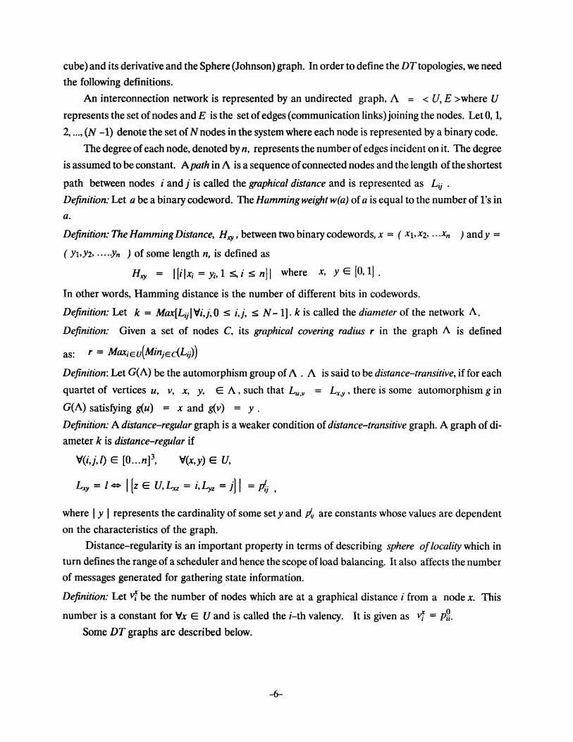
cube) and its derivative and the Sphere (Johnson) graph. In order to define the DTtopologies, we need

the following definitions.

An interconnection network is represented by an undirected graph, A = < U, E >where U

represents the set of nodes and E is the set of edges (communication links) joining the nodes. Let 0, 1,

2, ... , (N -1) denote the set of N nodes in the system where each node is represented by a binary code.

The degree of each node, denoted by n, represents the number of edges incident on it. The degree

is assumed to be constant. A path in A is a sequence of connected nodes and the length of the shortest

path between nodes i and j is called the graphical distance and is represented as L;j .

Definition: Let a be a binary codeword. The Hamming weight w(a) of a is equal to the number of l's in

a.

Definition: The Hamming Distance, Hxy, between two binary codewords, x = ( xhx2, .. . xn ) andy = ( YhY2· ·····Yn ) of some length n, is defined as

Hxy = l[ilx; = y;, 1 s, i s n) 1 where x, Y E [0, 1) .

In other words, Hamming distance is the number of different bits in codewords.

Definition: Let k = Max[LijiVi,j,O s i,j, s N-1]. k is called the diameter of the network A.

Definition: Given a set of nodes C, its graphical covering radius r in the graph A is defined

as: r = Max;eu(Minjec(Lij))

Definition: Let G(A) be the automorphism group of A . A is said to be distance-transitive, if for each

quartet of vertices u, v, x, y, E A , such that Lu,v = Lx,y , there is some automorphism gin

G(A) satisfying g(u) = x and g(v) = y .

Definition: A distance-regular graph is a weaker condition of distance-transitive graph. A graph of di­

ameter k is distance-regular if

V(i,j,l) E [O ... n]3, V(x,y) E U,

Lxy = I @ I {z E U, Lxz = i, Lyz = i} I = Jf;j ,

where I y I represents the cardinality of some set y and pij are constants whose values are dependent

on the characteristics of the graph.

Distance-regularity is an important property in terms of describing sphere of locality which in

turn defines the range of a scheduler and hence the scope ofload balancing. It also affects the number

of messages generated for gathering state information.

Definition: Let vf be the number of nodes which are at a graphical distance i from a node x. This

number is a constant for Vx E U and is called the i-th valency. It is given as vf = P3. Some DT graphs are described below.

-6-

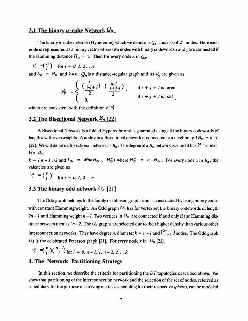
3.1 The binary n-cube Network Qn

The binary n-cube network (Hypercube), which we denote as Q", consists of 2" nodes. Here each

node is represented as a binary vector where two nodes with binary codewords x andy are connected if

the Hamming distance Hxy = 1. Then for every node x in Qn,

vf =( 7 ) for i = 0, 1, 2 .. n

and Lxy = Hx, and k = n. Qn is a distance-regular graph and its P;j are given as

( I ) ( n-1 ) i-j+1 i+j-1 2 -2- '

0,

which are consistent with the definition of vf .

3.2 The Bisectional Network Bn [22]

if i + j + I is even

if i + j + I is odd '

A Bisectional Network is a folded Hypercube and is generated using all the binary codewords of

lengthn with even weights. Anodexin aBisectional network is connected to a neighboryifHx, = n -1

[22]. We will denote a Bisectional network as Bn. The degree of a Bn network is nand it has 2n-l nodes.

For Bn,

k = ( n - 1 )12 and Lxy = Min(Hxy , Hi},) where Hi}, = n- Hxy . For every node x in Bn, the

valencies are given as

vf =(n,.) for i = 0, 1, 2 .. n.

3.3 The binary odd network On [21]

The Odd graph belongs to the family of Johnson graphs and is constructed by using binary codes

with constant Hamming weight. An Odd graph On has for vertex set the binary codewords of length

2n -1 and Hamming weight n -1. 1\vo vertices in On are connected if and only if the Hamming dis­

tance between them is 2n- 2. The On graphs are selected due to their higher density than various other

interconnection networks. They have degree n, diameter k = n -1 and (~ = f ) nodes. The Odd graph

03 is the celebrated Peterson graph [21]. For every node x in On [21],

0 =( ~ )( n .-1) . 1 1 z for z = 0, n -1, 1, n- 2, 2, .. k

4. The Network Partitioning Strategy

In this section, we describe the criteria for partitioning the DT topologies described above. We

show that partitioning of the interconnection network and the selection of the set of nodes, referred as

schedulers, for the purpose of carrying out task scheduling for their respective spheres, can be modeled

-7-

as a problem which is NP-hard. Subsequently, we propose an efficient solution, for partitioning and

finding the set of schedulers for these networks, based on a combinatorial structure called Hadamard

design. The proposed solution is "efficient" in that the size of the selected set of schedulers is consider­

ably small and it is of the order oflogarithm of the size of the networks. This results in a small number

of scheduling points and hence lower overhead resulting from message exchanges. We will denote this

set as C. Due to the smaller number of nodes in set C, the storage requirements for maintaining status

information about other members of the set Cis also small. At the same time, we show that the whole

network is uniformly covered and each sphere is symmetric and equal in size.

Based on this partitioning, we then propose a semi-distributed scheduling and load balancing

mechanism. In the proposed scheme, each sphere is assigned a scheduler which is responsible for (a)

assigning tasks to individual nodes of the sphere, (b) transferring load to other spheres, if required ,

and (c) maintaining the load status of the sphere and nodes. A scheduler is responsible for optimally

assigning tasks within its sphere depending upon the range of the scheduler which is, in turn, deter­

mined by the size of the sphere. Tasks can also migrate between spheres depending upon the degree of

imbalance in the loads of spheres. For the proposed scheme, each scheduler is located at the center of

each sphere. The details of the scheduling algorithm and information maintenance scheme are de­

scribed in section 5.

4.1. The Network Partitioning Problem

As mentioned above, C is the desired set of scheduling nodes. There can be various possible

options to select C and devise a semi-distributed scheduling strategy based on this set. However, the

performance of such a strategy depends on the "graphical locations" of the scheduler nodes (distances

between them) of C and the range of scheduling used by these nodes. The range of scheduling quanti­

fies the graphical distance within which a scheduler assigns tasks to the nodes of its sphere. In order to

characterize spheres and describe network partitioning, we need the following definitions.

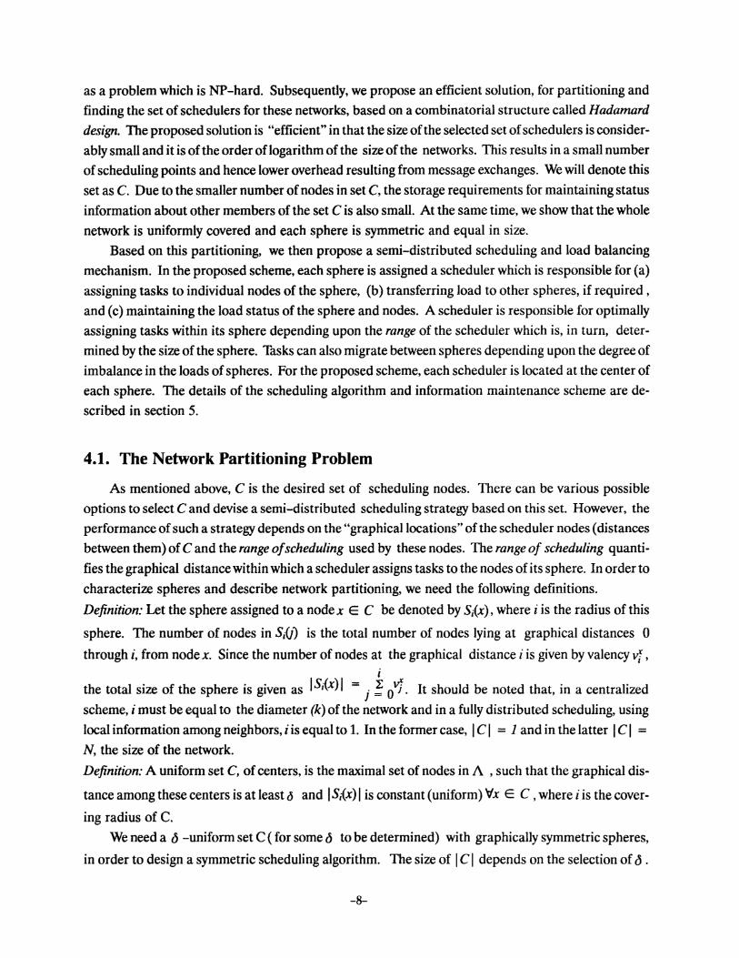
Definition: Let the sphere assigned to a nodex E C be denoted by S,{x), where i is the radius ofthis

sphere. The number of nodes in S,-(j) is the total number of nodes lying at graphical distances 0

through i, from node x. Since the number of nodes at the graphical distance i is given by valency vf , i

the total size of the sphere is given as IS,{x)l = j! 0vJ. It should be noted that, in a centralized

scheme, i must be equal to the diameter (k) of the network and in a fully distributed scheduling, using

local information among neighbors, i is equal to 1. In the former case, I C I = 1 and in the latter I C I =

N, the size of the network.

Definition: A uniform set C, of centers, is the maximal set of nodes in A , such that the graphical dis-

tanceamongthesecenters is at least() and IS;(x)l is constant(uniform) Vx E C, where iis the cover­

ing radius of C.

We need a d -uniform set C (for some d to be determined) with graphically symmetric spheres,

in order to design a symmetric scheduling algorithm. The size of I C I depends on the selection of d .

-8-

Intuitively, larger 6 yields smaller I C I, but spheres with larger size. It can also be observed that

reducing I C I increases the sphere size and vice versa. In addition, a number of other considerations

for load balancing are given below:

(1) Since a scheduler needs to distribute tasks to all the nodes in the sphere, the diameter of the sphere

should be as small as possible.

(2) I C I should be small, so that the global overhead of load balancing algorithm in terms of message

exchange among schedulers, maintenance of information and storage requirements is small.

(3) The size of the sphere should be small, firstly, because a scheduler (x) needs to send/receive I S;(x) I messages and, secondly, because information storage and maintenance requirements within the

sphere increase with the increase in sphere size.

We now describe the complexity of selecting a d -uniform

set (C).

Theorem 1: For a given value of 6 > 2,

(a) Finding a uniform set C in an arbitrary graph is NP-hard.

(b) Determining the minimum sphere size is also NP-hard.

Proof: (a) For the proof, see [39].

(b) Finding the minimum sphere size, I St_x) I Vx E C, requires us to determine the minimum value off,

which is equal to the covering radius of the set C. Since all the above topologies are represented using

binary codes, the problem of determining the set Cis equivalent to finding a sub code with the desired

covering radius in a code, say F. For Qn. F is the complete binary code. For a bisectional network, Bn,

F represents all the codewords of length n with even weights whereas for an odd graph, On. F repre­

sents a constant weight code of weight n with length n -1. However finding the covering radius of a sub

code, say C, in a code F is an NP-hard problem [30]. Since finding the minimum sphere size requires

determining the covering radius, the complexity of the whole problem will not be less than NP-hard.

Q.E.D.

The above theorem provides a rather pessimistic view for finding a set C for give F. However, we

present an interesting solution to select the set C in DT graphs using a combinatorial structure called

Hadamard Matrix. This matrix is described in the following section. The proposed solution for On with

6 = k, and for Qn and Bn with 6 = 1/k, is optimal in the sense that the set I C I is minimal.

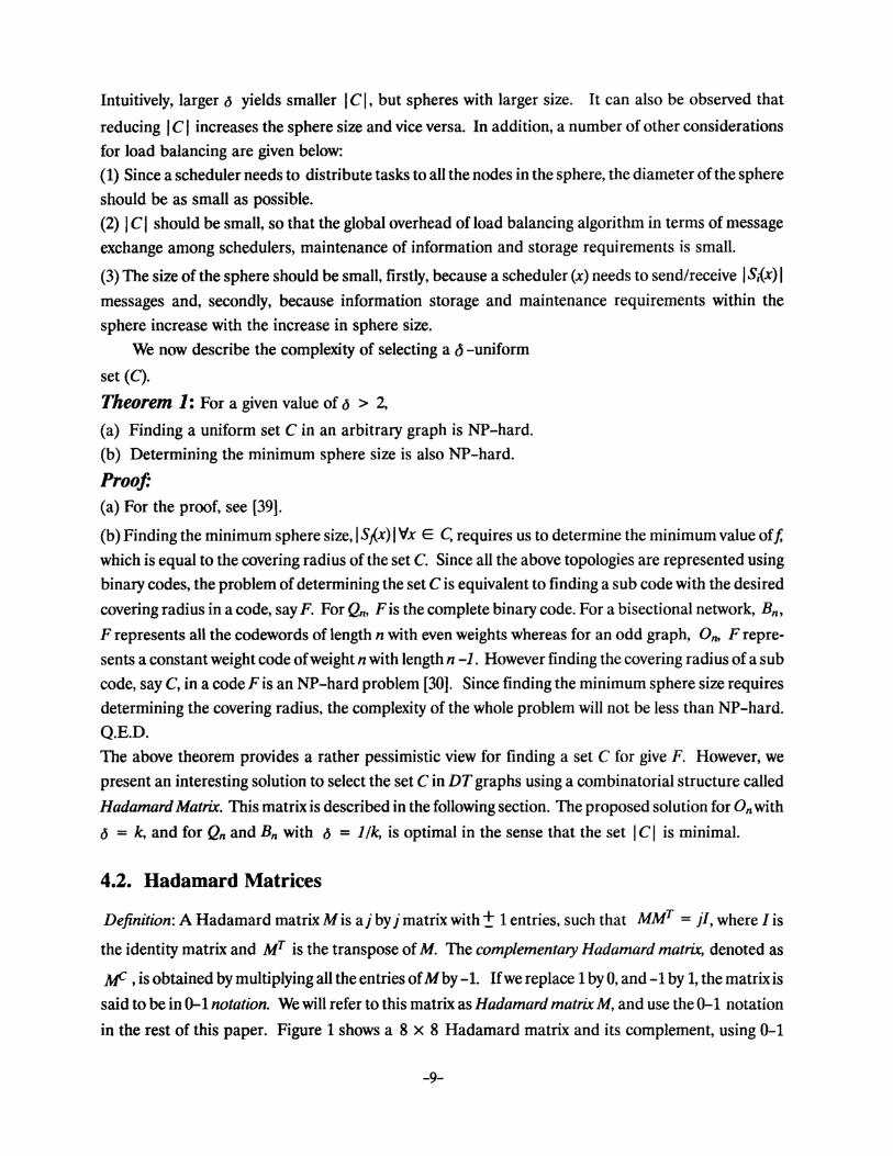
4.2. Hadamard Matrices

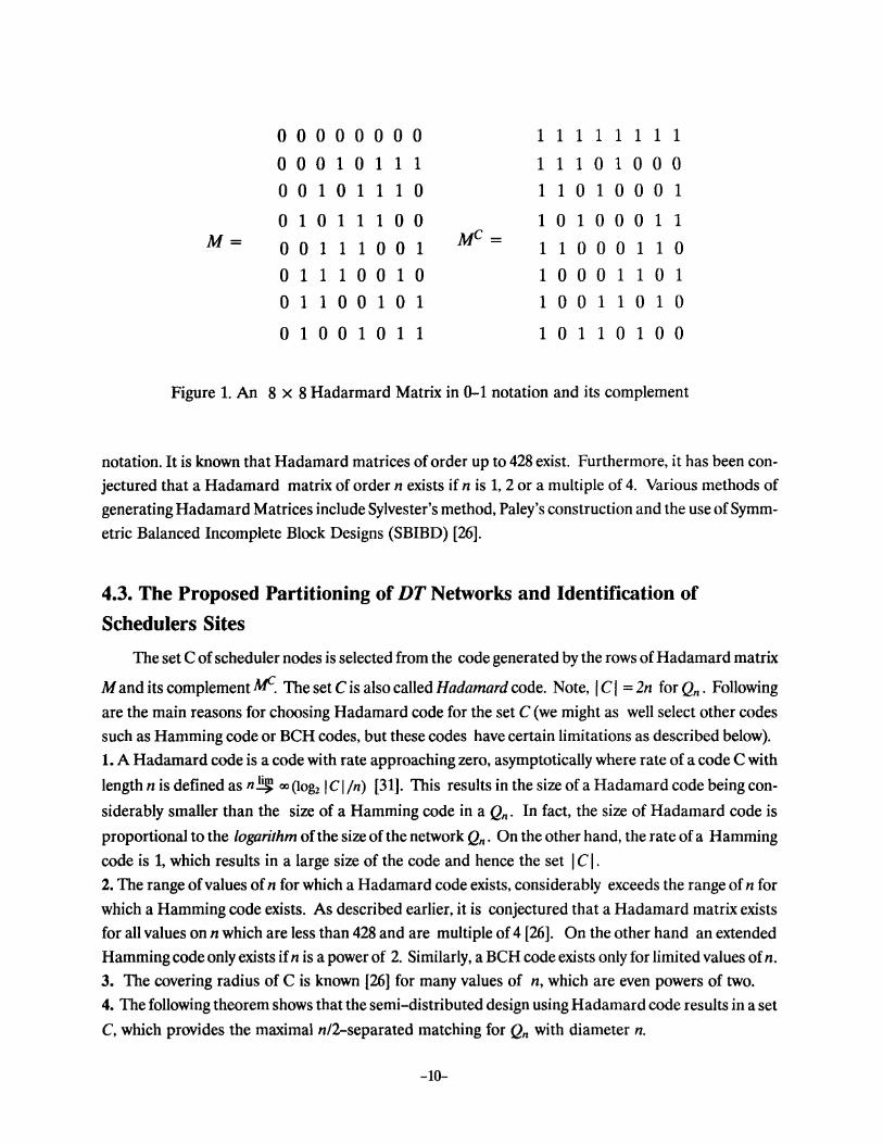
Definition: A Hadamard matrix M is aj by j matrix with± 1 entries, such that MMT = jl, where I is

the identity matrix and MT is the transpose of M. The complementary Hadamard matrix, denoted as

~ , is obtained by multiplying all the entries of Mby -1. If we replace 1 by 0, and -1 by 1, the matrix is

said to be in 0-1 notation. We will refer to this matrix as Hadamard matrix M, and use the 0-1 notation

in the rest of this paper. Figure 1 shows a 8 x 8 Hadamard matrix and its complement, using 0-1

-9-

0 0 0 0 0 0 0 0 1 1 1 1 1 1 1 1

0 0 0 1 0 1 1 1 1 1 1 0 1 0 0 0 0 0 1 0 1 1 1 0 1 1 0 1 0 0 0 1

0 1 0 1 1 1 0 0 1 0 1 0 0 0 1 1 M= 0 0 1 1 1 0 0 1 UC= 1 1 0 0 0 1 1 0

0 1 1 1 0 0 1 0 1 0 0 0 1 1 0 1

0 1 1 0 0 1 0 1 1 0 0 1 1 0 1 0

0 1 0 0 1 0 1 1 1 0 1 1 0 1 0 0

Figure 1. An 8 x 8 Hadarmard Matrix in 0-1 notation and its complement

notation. It is known that Hadamard matrices of order up to 428 exist. Furthermore, it has been con­

jectured that a Hadamard matrix of order n exists if n is 1, 2 or a multiple of 4. Various methods of

generating Hadamard Matrices include Sylvester's method, Paley's construction and the use of Symm­

etric Balanced Incomplete Block Designs (SBIBD) [26].

4.3. The Proposed Partitioning of DT Networks and Identification of

Schedulers Sites

The set C of scheduler nodes is selected from the code generated by the rows of Hadamard matrix

M and its complement AfC. The set Cis also called Hadamard code. Note, I C I = 2n for Qn. Following

are the main reasons for choosing Hadamard code for the set C (we might as well select other codes

such as Hamming code or BCH codes, but these codes have certain limitations as described below).

1. A Hadamard code is a code with rate approaching zero, asymptotically where rate of a code C with

length n is defined as n~ oo (log2 1 Cl fn) [31 ]. This results in the size of a Hadamard code being con­

siderably smaller than the size of a Hamming code in a Qn. In fact, the size of Hadamard code is

proportional to the logarithm of the size of the network Qn. On the other hand, the rate of a Hamming

code is 1, which results in a large size of the code and hence the set I C 1. 2. The range of values of n for which a Hadamard code exists, considerably exceeds the range of n for

which a Hamming code exists. As described earlier, it is conjectured that a Hadamard matrix exists

for all values on n which are less than 428 and are multiple of 4 [26]. On the other hand an extended

Hamming code only exists if n is a power of 2. Similarly, a BCH code exists only for limited values of n.

3. The covering radius of C is known [26] for many values of n, which are even powers of two.

4. The following theorem shows that the semi-distributed design using Hadamard code results in a set

C, which provides the maximal n/2-separated matching for Qn with diameter n.

-10-

Theorem 2: Letx,y E C. Then for Qn, Lxy = n/2. and Cis the maximal possible set, with n/2-sep­

arated matching.

Proof The Hamming distance between any two rows of a Hadamard matrix is n/2, that is for Qn,

Lxy = Hxy . In order to prove that the cardinality of the set is the maximum possible, assume the

contrary is true, and suppose there exists some codeword z, such that Hzx = n/2, for all x E C. A

simple counting argument reveals that there must be at least n(n-1 )14 l's at those n/2 columns where z

has O's. If these 1's are distributed among all rows ofM, then there are at least (n-l)-n(n-2)/[4(n-1)]

rows which can not be filled to obtain this Hamming distance. Therefore the node z is at a graphical

distance less than n/2 from these row. Q.E.D.

Due to the above mentioned advantages, we use Hadamard codes to construct the set C. Since, a

Hadamard code exists only when n is a multiple of 4, selection of the set C can be made by modifying

this untruncated code in various ways, to form the remainder of values. These modifications are de­

scribed below.

Case a: Qn with n mod 4 = 1. For this case, we consider the set C obtained from Hadamard

matrices M and~ (in 0-1 notation) of size n-1. The modified set C for the network under consider­

ation by appending an all O's and an alll's column, toM and~ respectively, at any fixed position, say

at extreme left.

Case b: Qn with n mod 4 = 2. This case is treated the same way as the Case (a), except we consider

the set C obtained from Hadamard matrices (in 0-1 notation) of size n-2 and append two columns 0

and 1 toM and 1 and 0 to~. However, the all O's row in M is augmented with bits 00 rather than with

bits 01. Similarly, the all l's row in ~ is augmented with bits 11 rather than with bits 10.

Case c: Qn with n mod 4 = 3. For this case, the set C consists of the rows of the truncated matrices

M and~ in 0-1 notation. The truncated matrices (in 0-1 notation) are generated by discarding the

all..Q row and column.

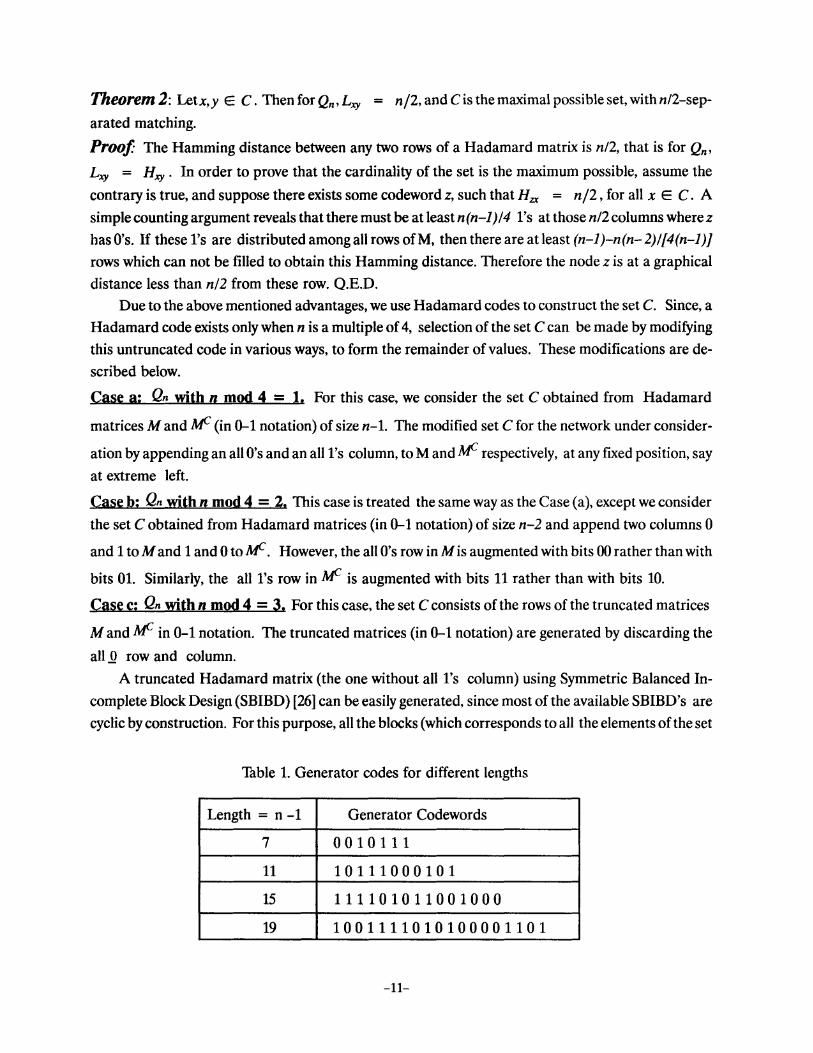
A truncated Hadamard matrix (the one without alll's column) using Symmetric Balanced In­

complete Block Design (SBIBD) [26] can be easily generated, since most of the available SBIBD's are

cyclic by construction. For this purpose, all the blocks (which corresponds to all the elements of the set

Table 1. Generator codes for different lengths

Length = n -1 Generator Codewords

7 0010111

11 10111000101

15 111101011001000

19 1001111010100001101

-11-

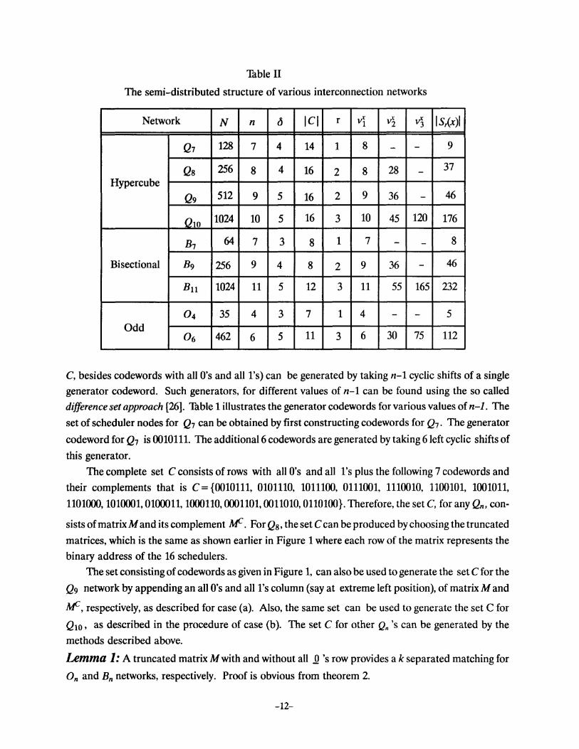
'Thble II

The semi-distributed structure of various interconnection networks

Network N n d ICI r v1 v2 vj IS,(x)l

Q, 128 7 4 14 1 8 - - 9

Qs 256 8 4 16 2 8 28 - 37

Hypercube Qg 512 9 5 16 2 9 36 - 46

Qw 1024 10 5 16 3 10 45 120 176

B, 64 7 3 8 1 7 - - 8

Bisectional Bg 256 9 4 8 2 9 36 - 46

Bn 1024 11 5 12 3 11 55 165 232

04 35 4 3 7 1 4 - - 5 Odd

11 6 30 75 112 06 462 6 5 3

C, besides codewords with all O's and a111's) can be generated by taking n-1 cyclic shifts of a single

generator codeword. Such generators, for different values of n-1 can be found using the so called

difference set approach [26]. 'Thble 1 illustrates the generator codewords for various values of n-1. The

set of scheduler nodes for Q1 can be obtained by first constructing codewords for Q1 . The generator

codeword for Q1 is 0010111. The additional6 codewords are generated by taking 6left cyclic shifts of

this generator.

The complete set C consists of rows with all O's and all l's plus the following 7 codewords and

their complements that is C= {0010111, 0101110, 1011100, 0111001, 1110010, 1100101, 1001011,

1101000, 1010001,0100011, 1000110,0001101,0011010, 0110100}. Therefore, the set C, for any Qn, con-

sists of matrixM and its complement JJC. For Q8, the set C can be produced by choosing the truncated

matrices, which is the same as shown earlier in Figure 1 where each row of the matrix represents the

binary address of the 16 schedulers.

The set consisting of codewords as given in Figure 1, can also be used to generate the set C for the

Q9 network by appending an all O's and alll's column (say at extreme left position), of matrix M and

JJC, respectively, as described for case (a). Also, the same set can be used to generate the set C for

Q10 , as described in the procedure of case (b). The set C for other Qn 'scan be generated by the

methods described above.

Lemma 1: A truncated matrix M with and without all .Q 's row provides a k separated matching for

On and Bn networks, respectively. Proof is obvious from theorem 2.

-12-

Lemma 1 can be used to partition an On graph into 2n -1 spheres. For instance, for 0 6, the gener­

ator codeword for 0 6 is 10111000101. The additional tO codewords generated by taking 10 left cyclic

shifts of this generator, constitute the set C for 0 6 • The set C for Bisectional networks Bn can be gener-

ated by taking only the matrix M for Qn (without JJC matrix ). For example, in the above example of

Q7 , we can take 8 rows of M to from the set C for B1 . Therefore in a Bn network the set Cis half the size

of that for Qn.

The topological characteristics and semi-distributed structure for Q7 , Qs , Q9 , Q10, B1, B9, Bu.

04 and 06 networks are summarized in Thble II which shows the number of nodes N, the degree n of

each node, the distance d between schedulers, the cardinality of the set C, the covering radius r, va­

lencies vf and the size of sphere I S,{x) I, for each network. In case the number of node is not divisible

by the number of schedulers ( as is the case for Bu), the difference in sphere sizes does not exceed 1.

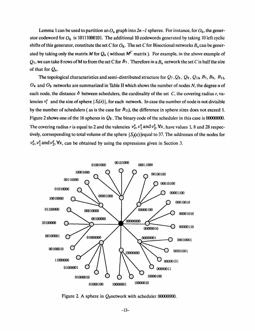
Figure 2 shows one of the 16 spheres in Qs . The binary code of the scheduler in this case is 00000000.

The covering radius r is equal to 2 and the valencies 0o. vi and~. 'Vx, have values 1, 8 and 28 respec­

tively, corresponding to total volume of the sphere I Sj(x) !equal to 37. The addresses of the nodes for

0a, vi and~. Vx, can be obtained by using the expressions given in Section 3.

1000 1000

00110000

01010000

10010000

01100000

10100000

00100001

00100010

11000000

01000001

01001000

01000010

01000100

00101000 000 11000

00010010

00001010

00000110

00010001

00001001

10000100

10000001 10000010

Figure 2. A sphere in Qsnetwork with scheduler 00000000.

-13-

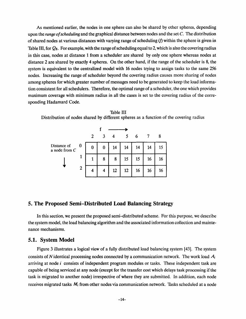
As mentioned earlier, the nodes in one sphere can also be shared by other spheres, depending

upon the range of scheduling and the graphical distance between nodes and the set C. The distribution

of shared nodes at various distances with varying range of scheduling (j) within the sphere is given in

'Thble Ill, for Qs. For example, with the range of scheduling equal to 2, which is also the covering radius

in this case, nodes at distance 1 from a scheduler are shared by only one sphere whereas nodes at

distance 2 are shared by exactly 4 spheres. On the other hand, if the range of the scheduler is 8, the

system is equivalent to the centralized model with 16 nodes trying to assign tasks to the same 256

nodes. Increasing the range of scheduler beyond the covering radius causes more sharing of nodes

among spheres for which greater number of messages need to be generated to keep the load informa­

tion consistent for all schedulers. Therefore, the optimal range of a scheduler, the one which provides

maximum coverage with minimum radius in all the cases is set to the covering radius of the corre­

sponding Hadamard Code.

'Thble m Distribution of nodes shared by different spheres as a function of the covering radius

f 2 3 4 5 6 7 8

0 0 14 14 14 14 15 Distance of a node from C

0

! 1

1 8 8 15 15 16 16

4 4 12 12 16 16 16 2

S. The Proposed Semi-Distributed Load Balancing Strategy

In this section, we present the proposed semi-distributed scheme. For this purpose, we describe

the system model, the load balancing algorithm and the associated information collection and mainte­

nance mechanisms.

5.1. System Model

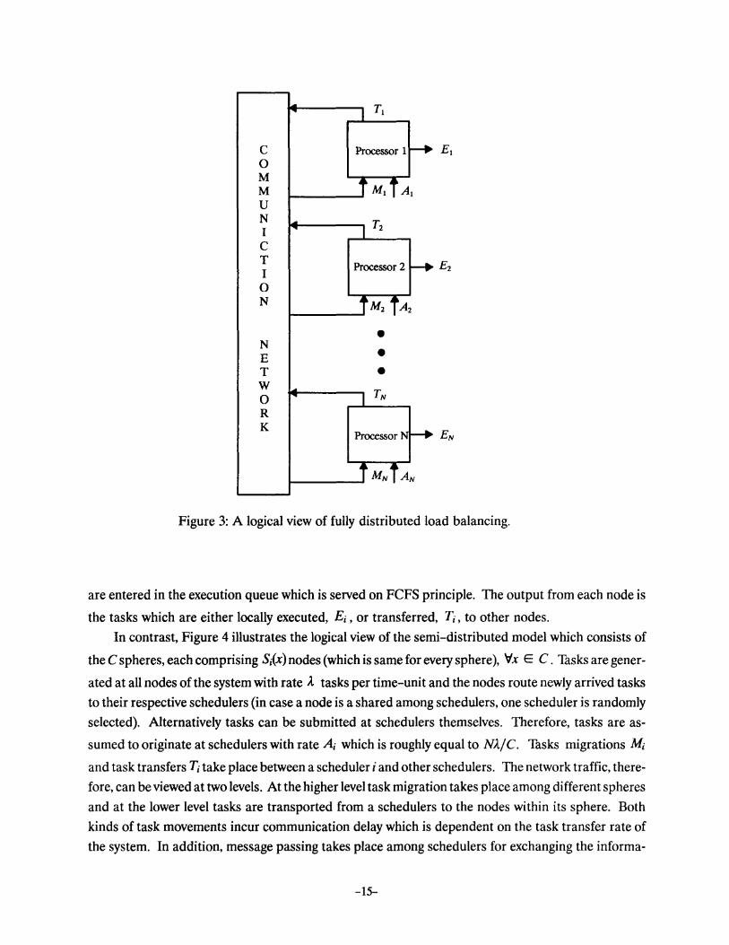
Figure 3 illustrates a logical view of a fully distributed load balancing system [43]. The system

consists of N identical processing nodes connected by a communication network. The work load A;

arriving at node i consists of independent program modules or tasks. These independent task are

capable of being serviced at any node (except for the transfer cost which delays task processing if the

task is migrated to another node) irrespective of where they are submitted. In addition, each node

receives migrated tasks M; from other nodes via communication network. Tasks scheduled at a node

-14-

Tt

c Processor 1 Et 0 M M At u N T2 I c T

Processor 2 E2 I 0 N A2

• N E • T • w

TN 0 R K

EN Processor

Figure 3: A logical view of fully distributed load balancing.

are entered in the execution queue which is served on FCFS principle. The output from each node is

the tasks which are either locally executed, E; , or transferred, T;, to other nodes.

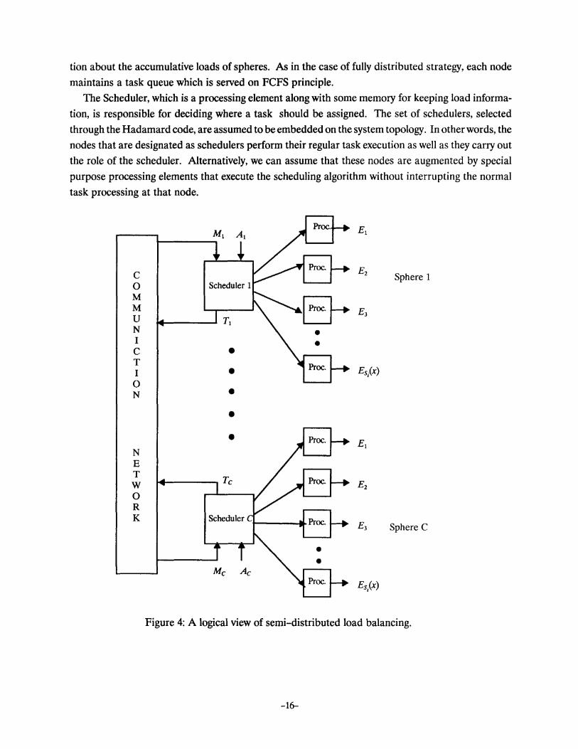
In contrast, Figure 4 illustrates the logical view of the semi-distributed model which consists of

the C spheres, each comprising S,{x) nodes (which is same for every sphere), 'Vx E C. Tasks are gener­

ated at all nodes ofthe system with rate A. tasks per time-unit and the nodes route newly arrived tasks

to their respective schedulers (in case a node is a shared among schedulers, one scheduler is randomly

selected). Alternatively tasks can be submitted at schedulers themselves. Therefore, tasks are as­

sumed to originate at schedulers with rate A; which is roughly equal to NA.jC. Tasks migrations Mi

and task transfers T; take place between a scheduler i and other schedulers. The network traffic, there­

fore, can be viewed at two levels. At the higher level task migration takes place among different spheres

and at the lower level tasks are transported from a schedulers to the nodes within its sphere. Both

kinds of task movements incur communication delay which is dependent on the task transfer rate of

the system. In addition, message passing takes place among schedulers for exchanging the informa-

-15-

tion about the accumulative loads of spheres. As in the case of fully distributed strategy, each node

maintains a task queue which is served on FCFS principle.

The Scheduler, which is a processing element along with some memory for keeping load informa­

tion, is responsible for deciding where a task should be assigned. The set of schedulers, selected

through the Hadamard code, are assumed to be embedded on the system topology. In other words, the

nodes that are designated as schedulers perform their regular task execution as well as they carry out

the role of the scheduler. Alternatively, we can assume that these nodes are augmented by special

purpose processing elements that execute the scheduling algorithm without interrupting the normal

task processing at that node.

c 0

£2 Sphere 1

M M £3 u N I c T I • Es;(x) 0 N •

• £1

N E T w £2 0 R K

£3 Sphere C

Figure 4: A logical view of semi-distributed load balancing.

-16-

5.2. State Information Exchange

The state information maintained by a scheduler is the accumulative load of its sphere which in

turn is the total number of tasks being serviced in that sphere at that time. This load index is adjusted

every time a task enters a sphere or finishes execution. In addition, a linked list is maintained in a non

decreasing order which sorts the nodes of sphere according to their loads. The load of a node is the

number of tasks in the execution queue of that node. The first element of the list points to the most

lightly loaded node of the sphere. The list is adjusted whenever a task is scheduled at a node or a task

finishes its execution. It is possible that a node is shared by more than one scheduler. In that case, the

scheduler that assigns the task to the shared node informs other schedulers to update their linked lists

and load entries. Similarly, a node has to inform all of its schedulers whenever it finishes a task.

5.3. The Load Balancing Algorithm

As mentioned earlier, at the second level, load balancing is done optimally within the spheres by

schedulers. Because of the sorted list maintained by the scheduler, a task is always scheduled at a node

with the lowest load. At the higher level, load balancing is achieved by exchanging tasks among spheres

so that the cumulative load between spheres is also equalized. Whenever a scheduler receives a task

from the outside world or from another scheduler, it executes the scheduling algorithm. Associated

with the scheduling algorithm are two parameters, namely threshold-! and threshold-2 which are used

to decide task migration. The two thresholds are adjustable system parameters which are set depend­

ing upon a number of factors (described later). Threshold-! is the load of the most lightly loaded node

within the sphere when the task is not to be scheduled within the local sphere. Threshold-2 is the

difference between the cumulative load of the local sphere and the cumulative load of the remote

sphere when the task is to be migrated to a remote sphere. The load balancing algorithm is executed by

a schedulers at the time it receives a locally generated task. It consists of the following steps.

Step 1. Check the load value of the node pointed by the first element of the linked list. This load is the

most lightly loaded node in the local sphere.

Step 2. If the load of the most lightly loaded node is less than or equal to threshold-I, then go to step 3.

Otherwise go to step 6.

Step 3. Schedule the task at that node.

Step 4. Updated the linked list by adding the new load to the original value and adust the list accord­

ingly.

Step 5. Increment the accumulative load of the sphere. Stop.

Step 6. Check the accumulative load of other spheres.

Step 7. If the difference between the cumulative load of the local sphere and the cumulative load of the

most lightly loaded remote sphere is less than threshold-2, send the task to that remote sphere where t

is executed without further migration to any other sphere. If there are more than one such spheres,

select one randomly. If there is no such sphere, then go to step 3. Stop.

-17-

Threshold-1 determines whether the task should be scheduled in the local sphere or a remote

sphere should be considered for transferring the task. Suppose the load threshold is set to one. Then if

an idle node is available in the sphere, that node is obviously the best possible choice. Even if the most

lightly loaded node already contains one task in its local queue, the probability of that node becoming

idle during the time task migrates from the scheduler to that node, is high. The scheduler considers

task migration to another sphere only if the load of the most lightly loaded node in its sphere is greater

than the threshold-1. Threshold-2 determines if there is significant difference between the accumula­

tive load of the local sphere and that of the remote sphere. One of the remote spheres, which meets the

threshold-2 criteria, is randomly selected. The reason for selecting a sphere randomly is to avoid the

most lightly loaded sphere becoming a victim of task dumping from other spheres. Choice of the load

thresholds should be made according to the system load and the task transfer rate. In our simulation

study, the values for threshold-1 have been varied between 1 and 2 and threshold-2 is varied from 1 to

6. The reason for selecting two threshold is to reduce the complexity of the scheduling algorithm. The

algorithm stops at step 5 if a node with load less than threshold-1 is present in the local sphere. This

also avoids generation of unnecessary messages for information collection from other schedulers, as

shown in step 6 of the algorithm.

6. Performance Evaluation and Comparison

For the performance evaluation of the proposed strategy, we have simulated various DT networks

such as Q7 , Qs , Q9 , Qw, B7 , B9 and 06. The simulation package written for this purpose runs on an

Encore Multimax. For comparison we have selected the no load balancing strategy and a fully decen­

tralized strategy. For the no load balancing strategy, tasks arrive at all nodes of the system with a

uniform arrival rate and are executed on the FCFS basis, without any load balancing. In the fully

distributed strategy, the control is fully decentralized and every node executes the same load balancing

algorithm. Tasks can migrate between nodes depending upon the decision taken by the algorithm at

each individual node. When a task arrives at a node, that node gets the load status from its immediate

neighbors. The load status of a node is the number of tasks scheduled at that node. If the local load is

less than the load of the most lightly loaded neighbor, the task is executed locally. Otherwise the task is

migrated to the neighbor with the lowest load. A task is allowed to make many migrations until it finds

a suitable node or the number of migrations made by the task exceed a predefined transfer limit.

Several variants of this algorithm, such as Shortest [14], [44], Contracting Within Neighborhood [27] and

Greedy strategy [12] have also been reported. The basic idea behind this algorithm is to schedule the

task at a node with minimum load. We believe that, for a fully distributed strategy, load exchange

between neighbors is both realistic and efficient - as pointed out in a comparison [27] where this

strategy is found to perform better than another fully distributed strategy known as Gradient Model

[28]. For simulation, task arrival process has been modeled as a Poisson process with average arrival

rate of A. tasks/unit-time which is identical for all nodes. The execution and communication times of

-18-

tasks have been assumed to be exponentially distributed with a mean of 1/ 1-ls time-units/task and

1/ !Jc time-units/task, respectively. The performance measures selected are mean response time of a

task and average number of control messages generated per task. In each simulation run, 20,000 to

100,000 tasks were generated depending upon the size of the network. The steady-state results are

presented with 95 percent confidence interval, with the size of the interval varying up to 5 percent of the

mean value of a number of independent replications. Extensive simulations have been performed to

determine the impact of the following parameters:

• The system load.

• The channel communication rate.

• Size and topology of the network.

• Comparison with other schemes.

The detail of the impact of these parameters is given in the following sections.

6.1. Response Time Performance

The mean response time of a task is the major performance criteria. 1b analyze the impact of

system load, defined as l/l.t, on mean response time, the system load is varied from 0.1 to 0.9. The

parameters selected in simulation are those that produced the best achievable performance for both

strategies. For different networks, the task transfer limit for the fully distributed strategy, for instance,

is equal to the diameter which produced the best results through simulation.

The communication delay incurred during task migration drastically effects the task response

time and a higher value of task transfer rate benefits both the strategies. However, to make meaning­

ful and fair comparisons and not ignoring the impact of communication delay at all, the task transfer

rate is selected as 20 task/time-unit compared to service rate of 1 task/time-unit. Nevertheless, the

impact of transfer delay, with higher and lower values of task transfer rates, is evaluated separately and

is presented in section 6.4.

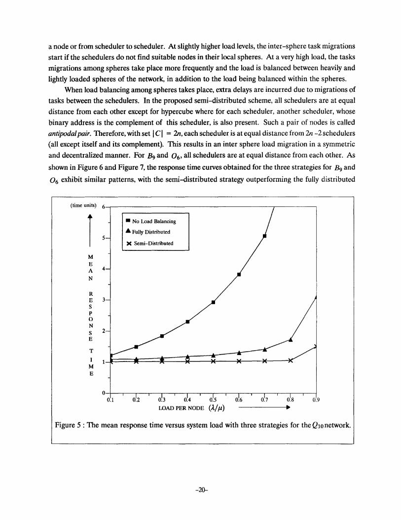
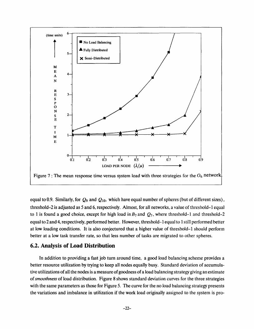
Figure 5, 6, and 7 show the average response time curves versus varying load condition for Q1o, B9 and 0 6 , respectively. Both fully and semi-distributed strategies yield a significant improvement

in response time over the no load balancing strategy at all loading conditions. For Q10, consisting of

1024 nodes, the average response time of the proposed semi-distributed strategy is superior to the fully

distributed strategy, at all loading conditions as shown in Figure 5. It is to be noted that for utilization

ratio up to 0.8, the response time curve with semi-distributed strategy is rather smooth and the average

response time is almost equal to 1.0, which is in fact the average service time of a task. This implies that

with the semi-distributed strategy the load balancing is optimal and tasks are serviced virtually with­

out any queuing delays. This is due to the fact that under low loading conditions, a scheduler is usually

able to find a node whose load index is less than or equal to threshold-1 which is set to one in this case.

For Q10, the sphere size is 176 and the probability of finding an idle node in a sphere is very high. In

other words, the scheduler always makes use of an idle node in its own sphere. The only delay incurred

before a task gets executed is the communication delay resulting from task transfer from a scheduler to

-19-

a node or from scheduler to scheduler. At slightly higher load levels, the inter-sphere task migrations

start if the schedulers do not find suitable nodes in their local spheres. At a very high load, the tasks

migrations among spheres take place more frequently and the load is balanced between heavily and

lightly loaded spheres of the network, in addition to the load being balanced within the spheres.

When load balancing among spheres takes place, extra delays are incurred due to migrations of

tasks between the schedulers. In the proposed semi-distributed scheme, all schedulers are at equal

distance from each other except for hypercube where for each scheduler, another scheduler, whose

binary address is the complement of this scheduler, is also present. Such a pair of nodes is called

antipodal pair. Therefore, with set I C I = 2n, each scheduler is at equal distance from 2n -2 schedulers

(all except itself and its complement). This results in an inter sphere load migration in a symmetric

and decentralized manner. For B9 and 0 6 , all schedulers are at equal distance from each other. As

shown in Figure 6 and Figure 7, the response time curves obtained for the three strategies for B9 and

0 6 exhibit similar patterns, with the semi-distributed strategy outperforming the fully distributed

(time units) 6_,...-----------------------r---------,

l M

E A

N

R E s p 0 N s E

T

I M E

5

4

3

2

• No Load Balancing

.A. Fully Distributed

)( Semi-Distributed

01~--~~--~~~~--r--r--~~-,-~-~--r--r--~~

0.1 ~4 ~5 ~6 0.9

LOAD PER NODE (A./p.)

Figure 5 : The mean response time versus system load with three strategies for the Q10 network.

-20-

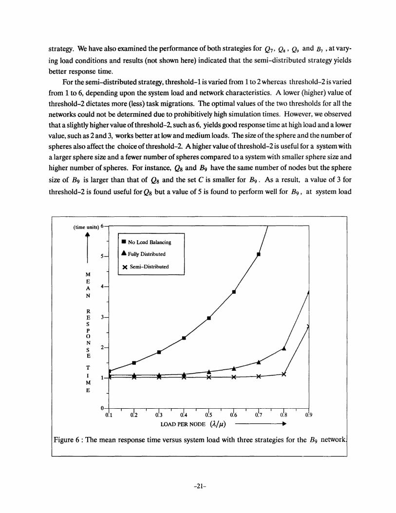
strategy. We have also examined the performance of both strategies for Q7 , Q8 , Q9 and B7 , at vary­

ing load conditions and results (not shown here) indicated that the semi-distributed strategy yields

better response time.

For the semi-distributed strategy, threshold-1 is varied from 1 to 2 whereas threshold-2 is varied

from 1 to 6, depending upon the system load and network characteristics. A lower (higher) value of

threshold-2 dictates more (less) task migrations. The optimal values of the two thresholds for all the

networks could not be determined due to prohibitively high simulation times. However, we obsetved

that a slightly higher value of threshold-2, such as 6, yields good response time at high load and a lower

value, such as 2 and 3, works better at low and medium loads. The size of the sphere and the number of

spheres also affect the choice of threshold-2. A higher value of threshold-2 is useful for a system with

a larger sphere size and a fewer number of spheres compared to a system with smaller sphere size and

higher number of spheres. For instance, Q8 and B9 have the same number of nodes but the sphere

size of B9 is larger than that of Q8 and the set C is smaller for B9 . As a result, a value of 3 for

threshold-2 is found useful for Qs but a value of 5 is found to perform well for B9 , at system load

(time units) 6

l • No Load Balancing

5 .t. Fully Distributed

)( Semi-Distributed

M E A 4

N

R E 3 s p 0 N s 2

E

T I 1 M E

0.1 0.2 0.3 0.4 0.5 0.6 0.8 0.9

WAD PER NODE (A/ /l)

Figure 6 : The mean response time versus system load with three strategies for the B9 network

-21-

(time units) 6

l • No Load Balancing

A Fully Distributed 5

X Semi-Distributed

M E A 4

N

R E 3 s p 0 N s 2 E

T

M 1

E

0 0.1 0.9

LOAD PER NODE ().j p)

Figure 7 : The mean response time versus system load with three strategies for the 06 network

equal to 0.9. Similarly, for Q9 and Q10 , which have equal number of spheres (but of different sizes),

threshold-2 is adjusted as 5 and 6, respectively. Almost, for all networks, a value of threshold-1 equal

to 1 is found a good choice, except for high load in B7 and Q7 , where threshold-1 and threshold-2

equal to 2 and 4, respectively, performed better. However, threshold-1 equal to 1 still performed better

at low loading conditions. It is also conjectured that a higher value of threshold-1 should perform

better at a low task transfer rate, so that less number of tasks are migrated to other spheres.

6.2. Analysis of Load Distribution

In addition to providing a fast job turn around time, a good load balancing scheme provides a

better resource utilization by trying to keep all nodes equally busy. Standard deviation of accumula­

tive utilizations of all the nodes is a measure of goodness of a load balancing strategy giving an estimate

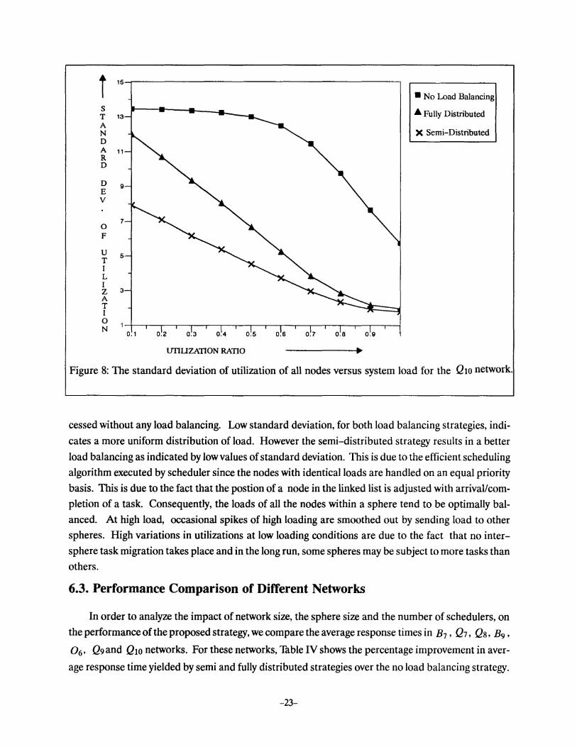
of smoothness of load distribution. Figure 8 shows standard deviation curves for the three strategies

with the same parameters as those for Figure 5. The curve for the no load balancing strategy presents

the variations and imbalance in utilization if the work load originally assigned to the system is pro-

-22-

s T 13 A N D A 11 R D

D E v

0 F

9

7

5

3

u T I L I z A T I 0 N 1-r~--r-.--.~-.--~.---~--.-.-.--.-.--.-.-~

0.1

UTIUZATION RATIO

• No Load Balancing

.t. Fully Distributed

X Semi-Distributed

Figure 8: The standard deviation of utilization of all nodes versus system load for the Qto network.

cessed without any load balancing. Low standard deviation, for both load balancing strategies, indi­

cates a more uniform distribution of load. However the semi-distributed strategy results in a better

load balancing as indicated by low values of standard deviation. This is due to the efficient scheduling

algorithm executed by scheduler since the nodes with identical loads are handled on an equal priority

basis. This is due to the fact that the postion of a node in the linked list is adjusted with arrivaVcom­

pletion of a task. Consequently, the loads of all the nodes within a sphere tend to be optimally bal­

anced. At high load, occasional spikes of high loading are smoothed out by sending load to other

spheres. High variations in utilizations at low loading conditions are due to the fact that no inter­

sphere task migration takes place and in the long run, some spheres may be subject to more tasks than

others.

6.3. Performance Comparison of Different Networks

In order to analyze the impact of network size, the sphere size and the number of schedulers, on

the performance of the proposed strategy, we compare the average response times in B7 , Q7, Qs, B9 ,

0 6 , Q9and Q10 networks. For these networks, Table IV shows the percentage improvement in aver­

age response time yielded by semi and fully distributed strategies over the no load balancing strategy.

-23-

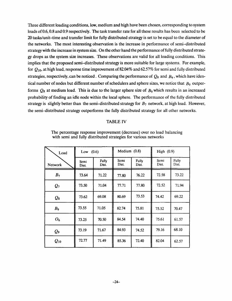
Three different loading conditions, low, medium and high have been chosen, corresponding to system

loads of0.6, 0.8 and 0.9 respectively. The task transfer rate for all these results has been selected to be

20 tasks/unit-time and transfer limit for fully distributed strategy is set to be equal to the diameter of

the networks. The most interesting observation is the increase in pedormance of semi-distributed

strategy with the increase in system size. On the other hand the pedormance of fully distributed strate­

gy drops as the system size increases. These observations are valid for all loading conditions. This

implies that the proposed semi-distributed strategy is more suitable for large systems. For example,

for Q10, at high load, response time improvement of 82.04% and 62.57% for semi and fully distributed

strategies, respectively, can be noticed. Comparing the performance of Q8 and B9 , which have iden­

tical number of nodes but different number of schedulers and sphere sizes, we notice that B9 outper­

forms Q8 at medium load. This is due to the larger sphere size of B9 which results in an increased

probability of finding an idle node within the local sphere. The performance of the fully distributed

strategy is slightly better than the semi-distributed strategy for B1 network, at high load. However,

the semi-distributed strategy outperforms the fully distributed strategy for all other networks.

TABLE IV

The percentage response improvement (decrease) over no load balancing with semi and fully distributed strategies for various networks

~ Low (0.6) Medium (0.8) High (0.9)

Semi Fully Semi Fully Semi Fully Dist. Dist. Dist. Dist. Dist. Dist. k

B1 73.64 71.22 77.80 76.22 72.58 73.22

Q7 73.50 71.04 77.71 77.80 72.52 71.94

Qs 73.62 69.08 80.69 73.53 74.42 69.22

B9 73.55 71.05 82.74 75.81 75.52 70.47

06 73.25 70.50 84.54 74.40 75.61 61.57

Q9 73.19 71.67 84.93 74.52 79.16 68.10

Qto 72.77 71.49 85.36 72.40 82.04 62.57

-24-

6.4. Sensitivity To Communication Delay

The response time performance of a load balancing strategy can degrade because of the commu­

nication delays incurred during task migration. Moreover, high transmission delay not only slows task

migration but also results in an increased queuing delay in the communication queues. The impact of

communication delay on the task response time is determined by the ratio of mean communication

delay to mean service time. If this ratio is high, load balancing does not prove beneficial since its

average response time may even exceed the response time obtained with no load balancing [32]. If fully

distributed load balancing is carried out with slow communication, the state of the system can change

by the time a task migration completes, and the task may have to be remigrated to another node. This

may result in task thrashing. a phenomenon in which tasks keep on migrating between nodes without

setting down. On the other hand, with the semi-distributed load balancing scheme, a task migrates

only from a scheduler to a node and/or from scheduler to scheduler. However, since both schemes are

susceptible to the communication rate of the underlying network, we present the response time per­

formance for varying task transfer rates at medium and high system load, for all seven networks.

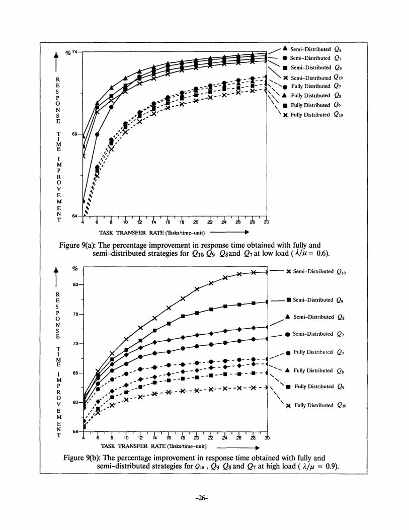
For Q10 Q9, Q8, and Q7, the curves for percentage improvement in average response time, over

the no load balancing strategy, versus varying task transfer rates, have been obtained with both the

strategies. These curves for low and high loads are shown in Figure 9(a) and Figure 9(b ), respectively.

These results also help us examine the performance of hypercube topology of varying size under differ­

ent loading and communication conditions. Task transfer rates are varied from 4 task/time-unit to 30

tasks/time-unit; by increasing the task transfer rate beyond 30 tasks/time-unit, the performance im­

provement has been found to be negligible. The results indicate that even at a very slow task transfer

rate, the response time improvement with the semi-distributed strategy is better than the improve­

ment gained with the fully distributed strategy. At system load equal to 0.6, the response time improve­

ment yielded by the fully distributed scheme decreases with increase in system size whereas for the

semi-distributed scheme, Qs and Q7 yield the best and the worst performances, respectively. How­

ever, all networks perform better with the semi-distributed strategy. At high load, the difference in the

performance of both strategies is significantly high. Figure 9(b) clearly indicates that the response

time improvement, with the proposed strategy, is enhanced for the larger systems. On the other hand,

with the fully distributed load balancing, the performance decreases with increase in system size.

From Figure 9(a), we also observe that, with the exception of Q7 , the other three networks perform

reasonably good under the semi-distributed scheme, even at very slow task transfer rate. In contrast,

Figure 9(b) indicates that the performance of the semi-distributed scheme keeps on increasing with

the increase in task transfer rate whereas the performance of the fully distributed scheme saturates if

the task transfer rate is increased beyond 20 tasks/time-unit.

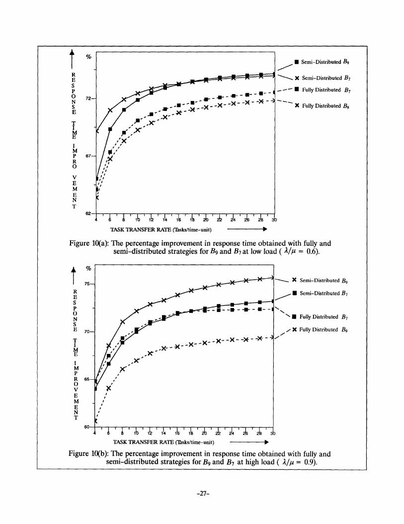
Figure lO(a) and Figure lO(b) present percentage response time improvement at low and high

load, respectively, for the two Bisectional networks, B9 and B7 • From Figure lO(a), we notice the pro­

posed scheme performs consistently better for B9 whereas it shows some dependency towards the task

-25-

- e Semi-Distributed Q7 t % 74-~------~=:;~;~~~~j~i~~9~ A Semi-Distributed Q8

~ • Semi-Distributed Q9

, ""- X Semi-Distributed Qut R E s p 0 N s E

T I M E

I M p R 0 v E M E N T

TASK TRANSFER RATE ('Thsksltime-unit)

',''e Fully Distributed Q7

~ '\' A Fully Distributed Qs

\~ • Fully Distnbuted Q9

'\ X Fully Distributed QlO

Figure 9(a): The percentage improvement in response time obtained with fully and semi-distributed strategies for Qtn Qg Qsand Q7 at low load ( A./ IJ. = 0.6).

t R E s p 0 N s E

T I M E

I M p R 0 v E M E N T

%

83

78

73

68

63

.,... e Fully Distributed Q7 ........ -.. -.. -·- -:--_ ... -... -•-• __ ... -.--·-- -- ....

, ..e, _ • ... _ -+- _ +- - •. _ -• _ -• _ ..... _ -11- _ , ........ A Fully Distributed Q8 ·- ... - . --· -- ' ,,' ... ~- __ ..... -- ' Q • ,.-: .. , -• _ * _ * _ ~-_ K-- )(- -)E- -)E-- '\ • Fully Distributed 9

,' .- )( _)(--* \ ,' .. , ,' - ' /J( :,:x- X Fully Distributed Qto , ,~ , . , ,

1 1

TASK TRANSFER RATE (Thsks/time-unit)

Figure 9(b ): The percentage improvement in response time obtained with fully and semi-distributed strategies for QlO , Qg Qs and Q1 at high load ( J..j p. = 0.9).

-26-

t R E s p 0 N s E

T I

r I M p R 0

v E M E N T

%

72

67

~ • Semi-Distributed B9

~---~t:::::..-:--.Jt'~llt='==Jl==Jt=:Jt==!~~ ............... X Semi-Distributed B1

--- • Fully Distributed B1 ---- ·-- ·--·----·-- .. - -)E- ->E-- ---- ... _ -• ---->E _-:>E--)(- -:>E- X Fully Distributed B9

.... -,)('-~ ... -- v-'

, '" ~--_,x--

,'x' I I

I I

.. ,' ,'X

I I I I

•' I I I I

•,' , ,

TASK TRANSFER RATE (Thsks!time-unit)

Figure lO(a): The percentage improvement in response time obtained with fully and semi-distributed strategies for B9 and B1 at low load ( A./ f.l = 0.6).

t %

75

R E s p 0 N s E 70

T I M E

I M p R 65 0 v E M E N T

60

I I

I

K'

,x--,X",

)(- -)(- -)(- -)E- ->E--'>I- -X--

-~-~

TASK TRANSFER RATE (Thsks/time-unit) ..

~ • Semi-Distributed B1

' ' ' • Fully Distributed B1

./ X Fully Distributed B9 ./

../

Figure lO(b): The percentage improvement in response time obtained with fully and semi-distributed strategies for B9 and B7 at high load ( A./ f.l = 0.9).

-27-

i R E s p 0 N s E

T I

if I M p R 0 v E M E N T

%

70

I I

I

I I

I

I I

I I

, , ,

TASK TRANSFER RATE (Disks/time-unit)

---- X Fully Distributed

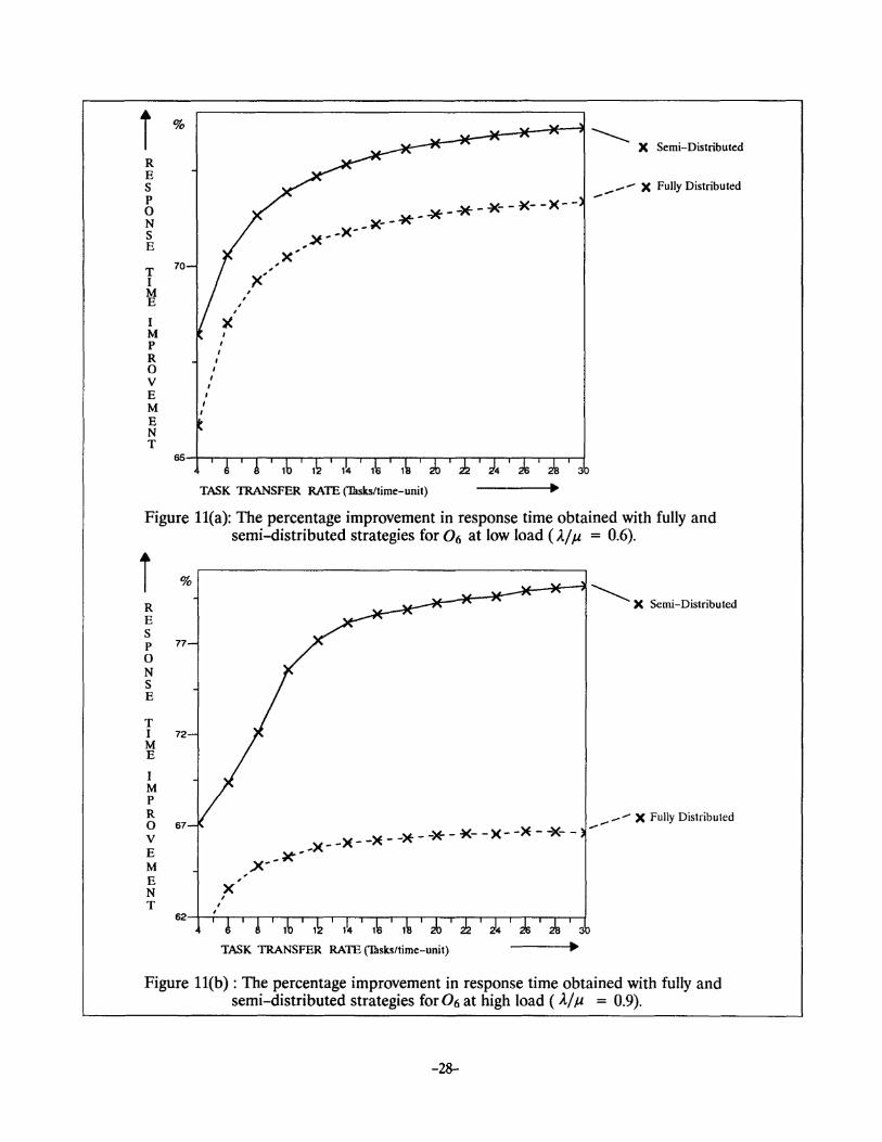
Figure ll(a): The percentage improvement in response time obtained with fully and semi-distributed strategies for 0 6 at low load (A./ It = 0.6).

i R E s p 0 N s E

T

%

77

I 72 M E

I M p R 0 v E M E N T

67

x ' '

~.-1~~-*"-74r-"l ~X Semi-Distributed

_ .... X Fully Distributed .... -

)(- -)(- ->E- ->t- ->E-- ~-- )(- ->E- -i<--

,,x--~ --

~-r.'~-..-.-.. -.-..-~~--,--~,.-,.-,-,~~

Figure ll(b) : The percentage improvement in response time obtained with fully and semi-distributed strategies for 06 at high load ( l/ It = 0.9).

-28-

transfer rate for the B7 network. Earlier we noticed the same results for the Q1 , as shown in Figure

9(a), which lead to the conclusion that the smaller systems are more susceptible to task transfer rate,

under the proposed scheme. At high load, the response time improvements, obtained with both the

strategies are almost identical for the B7 network whereas the results are substantially different for

the B9 network. This reconfirms our conclusion that larger systems perform better under the pro­

posed strategy. The results shown in Figure ll(a) and Figure ll(b) for the 0 6 network also reconfirm

these results. These results also indicate that the gain in performance over no load balancing is even

better at high loading conditions.

6.5. The Message Overhead

The exchange of control information, which is essential for any load balancing algorithm, should

be carried out in an efficient way. In order to design a state information collection policy, one must

decide what type of information is required and how frequently that information should be inter­

changed. In addition, the information exchange policy should meet at least two objectives. The first

objective is to ensure that the information is accurate and sufficient! enough for the proper operation

of the scheduling algorithm. The second objective should be to limit the amount and frequency of the

information interchange within an acceptable level so that the resulting overhead is not too high. In a

completely decentralized policy, every node needs to maintain its own view of the system state such as

load status of neighbors. Consequently, the frequency and amount of these message exchanges can

cause extra channel traffic which can slow down the information exchange activity as well as normal

task migration. In order to have an updated information, the control messages need to be handled on

some form of priority basis. If a task makes a large number of migrations, all the intermediate nodes

generate extra messages and the overhead increases proportionally. Clearly a trade-off is at work

here. One needs to have sufficient information available to the scheduler while reducing the resulting

overhead. In addition to average task response time, this message overhead, therefore, is another per­

formance measure of a load balancing policy. One of the goals of the proposed strategy is to reduce

this control overhead. We define this overhead as the average number of messages generated per task

(this was calculated by dividing the total number of generated messages by the total number of tasks).

As explained in section 5, in the proposed strategy, this overhead results from two types of informa­

tions , that is, the load status of individual nodes within the spheres and the accumulative load of the

spheres. If a node is shared among more than one spheres, then the scheduler assigning the task to that

node informs the schedulers of other spheres to update their load entries for that node. Upon finishing

a task, a node informs all of its schedulers. This results in a consistent load information about all the

nodes and yet the number of messages generated is considerably small. At the sphere level, a scheduler

communicates with other schedulers only when it considers a task migration.

As mentioned earlier the number of schedulers is only of the order of log N. Therefore, the num­

ber of such messages is also small. However, the number of messages also depend on other factors

such as system load, the two thresholds and partitioning strategy which in turn determines the size of

-29-

N u M E R

0 F

M E s s

- Semi-Distributed c:::J Fully Distributed

A 0~-+~~~~~~~~~~~ G E s 0.1 0.2 0.3 0.4 0.5 0.6 0. 7 0.8 0.9 1.0

UTILIZATION RATIO •

Figure 12: The average number of messages per task versus system load for B1.

r N u M E R

0 F

M E s s A G E s

- Semi-Distributed c:::J Fully Distributed

0.1 0.2 0.3 0.4 0.5 0.6 0.7 0.8 0.9 1.0 UTILIZATION RATIO •

Figure 13: The average number of messages per task versus system load for Q7.

N u M E R

0 F

M E s s A G E s

Semi-Distributed Fully Distributed

0.1 0.2 0.3 0.4 0.5 0.6 0.7 0.8 0.9 1.0 UTIUZATIONRATIO •

Figure 14: The average number of messages per task versus system load for Qs.

-30-

the sphere, number of spheres and sharing of nodes among spheres. It is difficult to analyze the com­

bined effect of all these factors, however, simulation results presented in this section enable us to

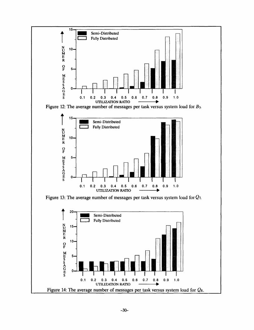
briefly explain the impact of these factors, individually. In Figure 12 to 18, the average number of

control messages, with varying system load, are plotted for B1, Q1, Qs, Bg, Qg, Q10 and 06 net­

works, respectively. These figures indicate that the overhead is low at low loading conditions. This is

due to the fact, that at low load, the schedulers do not communicate with each other since a suitable

node is available within the local sphere, most of the time. Consequently, the overhead at low loading

condition is only a result of message exchanges between nodes and schedulers, whenever the load sta­

tus of a shared node is updated among schedulers.

As the load increases from medium to high, the probability of finding a task within a local sphere

decreases and scheduler start communicating with each other, depending upon the values of the two

thresholds. If the two thresholds have high values, then the frequency of such information exchange

decreases and consequently the overhead decreases. However, this can result in a higher response

time. It should be pointed out that the two threshold for the results depicted in Figure 12 to Figure 18

have been adjusted not with the objective of reducing the overhead; rather these results present the

overhead with threshold values that produced good response times. In contrast, the fully distributed

strategy induces high overhead which almost doubles the overhead incurred by the semi-distributed

strategy, except for 0 6 and Qto where the overhead resulting from the semi-distributed strategy is

high due to high degree of sharing of nodes among spheres.

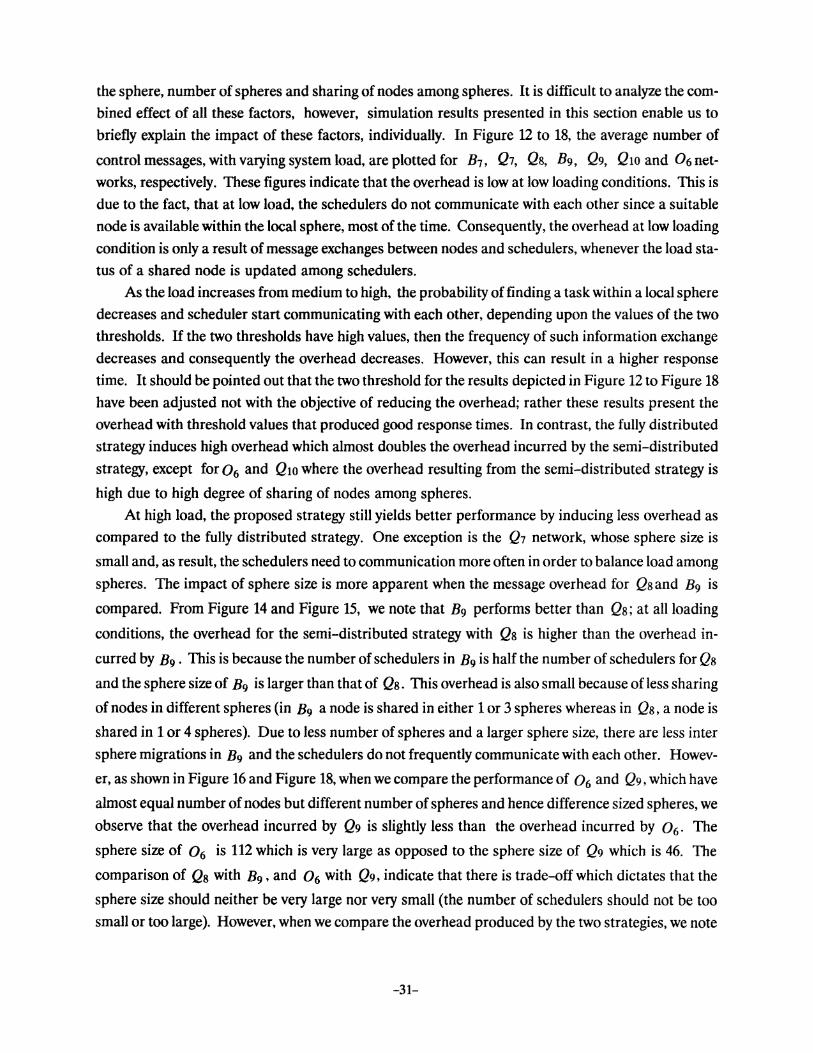
At high load, the proposed strategy still yields better performance by inducing less overhead as

compared to the fully distributed strategy. One exception is the Q7 network, whose sphere size is

small and, as result, the schedulers need to communication more often in order to balance load among

spheres. The impact of sphere size is more apparent when the message overhead for Qs and B9 is

compared. From Figure 14 and Figure 15, we note that B9 performs better than Qs; at all loading

conditions, the overhead for the semi-distributed strategy with Qs is higher than the overhead in­

curred by B9 • This is because the number of schedulers in B9 is half the number of schedulers for Qs

and the sphere size of B9 is larger than that of Qs. This overhead is also small because of less sharing

of nodes in different spheres (in B9 a node is shared in either 1 or 3 spheres whereas in Qs, a node is

shared in 1 or 4 spheres). Due to less number of spheres and a larger sphere size, there are less inter

sphere migrations in B9 and the schedulers do not frequently communicate with each other. Howev­

er, as shown in Figure 16 and Figure 18, when we compare the performance of 0 6 and Qg, which have

almost equal number of nodes but different number of spheres and hence difference sized spheres, we

observe that the overhead incurred by Q9 is slightly less than the overhead incurred by o6 . The

sphere size of 0 6 is 112 which is very large as opposed to the sphere size of Q9 which is 46. The

comparison of Qs with B9 , and 0 6 with Qg, indicate that there is trade-off which dictates that the

sphere size should neither be very large nor very small (the number of schedulers should not be too

small or too large). However, when we compare the overhead produced by the two strategies, we note

-31-

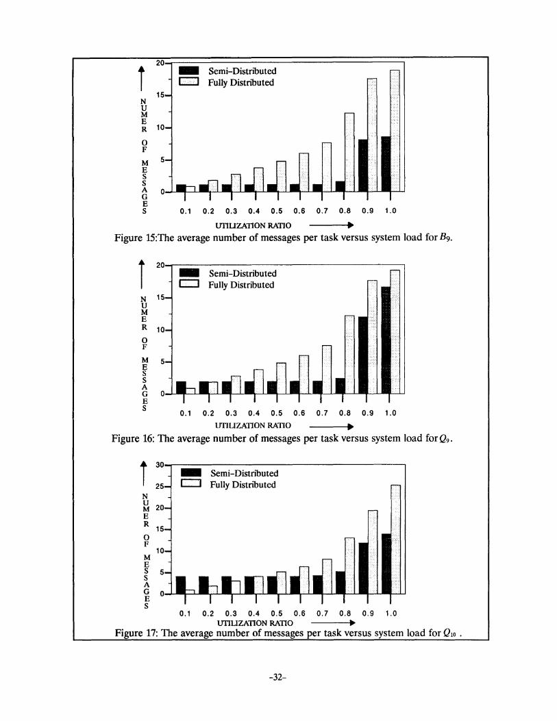
r N u M E R

0 F

M E s s A G E s

20 - Semi-Distributed c:J Fully Distnbuted

0.1 0.2 0.3 0.4 0.5 0.6 0.7 0.8 0.9 1.0

UTILIZATION RATIO liJJo

Figure 15:The average number of messages per task versus system load for B9.

r 20 - Semi-Distributed

c:J Fully Distributed N 15 u M E R 10 0 F

M 5 E s s A G 0 E s

0.1 0.2 0.3 0.4 0.5 0.6 0.7 0.8 0.9 1.0

UTILIZATION RATIO 1iJJo

Figure 16: The average number of messages per task versus system load for Q9.

r 30 - Semi-Distributed 25 c:J Fully Distributed

N u

20 M E R

15 0 F

10 M E s 5 s A G 0 E s

0.1 0.2 0.3 0.4 0.5 0.6 0.7 0.8 0.9 1.0 UTILIZATION RATIO IJJo

Figure 17: The average number of messages per task versus system load for 01o .

-32-

I 20 - Semi-Distributed

c::J Fully Distributed

N 15 u M E R 10 0 F

M 5 E s s A G 0 E s 0.1 0.2 0.3 0.4 0.5 0.6 0.7 0.8 0.9 1.0

UTILIZATION RATIO • Figure 18:The average number of messages per task versus system load for06.

that the proposed strategy consistently performs better than the fully distributed strategy. As shown in

Figure 12, the conclusion is valid even for B7 where sphere size is very small. The conclusion also

holds for Q10, as shown in Figure 17, where the sphere size is very large.

7. Conclusions

In this paper, we have proposed a new load balancing approach for large-scale multicomputer

systems and have presented the concept of a semi-distributed control. The study was centered around

a class of interconnection structures which are distance-transitive. The use of Hadamard matrix re­

sults in an efficient strategy for partitioning these systems for load balancing. We have evaluated the

performance of the proposed strategy through an extensive simulation study. By comparing with a

fully distributed strategy, we have shown that the proposed strategy yields a better performance in

terms of average response time, resource utilization and average number of control messages gener­

ated.

One of the conclusions drawn from the comparative performance of Hypercube, Bisectional and

Odd graphs is that the network topology has a rather low effect on response time. In other words, for

the three kinds of graphs under study, the proposed strategy using different number of spheres with

different sizes performs equally good. This is true for a wide range of task transfer rate of the commu­

nication network. We also notice that the proposed strategy performs better as the system size in­

creases. This was observed by comparing the performance of Hypercube as well as Bisectional graphs.

The proposed partitioning strategy results in a small number of spheres which remain of E>( log N ). For instance the number ofspheres for Qu is 24 and remains the same for Q12• Q13 and Q14·

The next higher value of the number of spheres is 32. Similar techniques are applied to Bisectional and

Odd graphs.

-33-

References

[1] Ishfaq Ahmad, Arif Ghafoor and Kishan Mehrotra, "Performance Prediction for Distributed

Load Balancing in Multicomputer Systems," Thchnical Report no. SU-CIS-91-12, School of

Computer and Information Science, Syracuse University, April1991.

[2] William C. Athas and Charles L. Seitz, "Multicomputers: Message-Passing Concurrent Comput­

ers," IEEE Computer, August 1988, pp. 9-24.

[3] E. Bannai and'[ Ito, Algebraic Combinatorics and association schemes. Benjamin-Cummings

(1984).

[4] Amnon Barak and Amnon Shiloh," A Distributed Load balancing Policy for a Multicomputer,"

Software Practice and Experience, vol. 15(9), Sept. 1985, pp. 901-913.

[5] Katherine M. Baumgartner, Ralph Kling and Benjamin Wah," A Global Load Balancing Strategy

for a Distributed System," in Proc. of Int'l. Cont on Future Trends in Distributed Computing Sys­tems, Hong Kong, 1988 pp. 93-102.

[6] Shahid H. Bokhari, "Dual Processor Scheduling with Dynamic Reassignments," IEEE Trans. on Software Eng. vol. SE-5, July 1979, pp. 341-349.

[7] Nicholas S. Bowen, Christos Nikolaou and Arif Ghafoor, "On the Assignment Problem of Arbi­

trary Process Systems to Heterogeneous Distributed Computer Systems," To appear in IEEE

Trans. on Computers.

[8] Raymong M. Bryant and Raphael A. Finkel, "A Stable Distributed Scheduling Algorithm," in

Proc. of 2nd Int'l. Cont on Distributed Computing Systems, 1981, pp. 314-323.

[9] Thomas L. Casavant and John G. Kuhl, "Analysis of Three Dynamic Load-Balancing Strategies

with Varying Global Information Requirements," in Proc. of 7-th Int'l. Cont on Distributed Com­

puting Systems, 1987, pp. 185-192.

[10] 'Ibny F. Chan,"Hierarchical Algorithms and Architectures for Parallel Scientific Computing," in

Int'l. Conference on Supercomputing, 1990, pp. 318-329.

[11] Yaun-Chien Chow and Walter H. Kohler,"Models for Dynamic Load balancing in Homogeneous

Multiple Processor Systems," IEEE Trans. on Computers, vol. c-36, no. 6, May, 1982, pp. 667-679.

[12] Shyamal Chowdhury, ''The Greedy Load Sharing Algorithm," Journal of Parallel and Distributed Computing, no. 9, May 1990, pp. 93-99.

[13] DARPA, "Strategic Computing: New Generation Computing technology," Defence Advance Re­search Project Agency, Arlington, VA, Oct. 1983

[14] Derek L. Eager, Edward D. Lazowska and John Zahorjan,"Adaptive Load Sharing in Homoge­

neous Distributed Systems," IEEE Trans. on Software Eng. ,vol. SE-12, May 1986, pp. 662-675.

[15] ,"A Comparison of Receiver Initiated and Sender Initiated Adaptive

Load Sharing," ACM Performance Evaluation, March 1986, pp. 53-68.

[16] Kemal Efe and Bojan Groselj, "Minimizing Control Overhead in Adaptive Load Sharing," in

Proc. of 9-th Inti. Cont on Distributed Computing Systems, 1989, pp. 307-315

-34-

[17] Ahmed K. Ezzat, R. Daniel Bergerson and John L. Pokoski, "Task Allocation Heuristics for Dis­

tributed Computing Systems, "in Proc. of 6-th Int'l. Cant on Distributed Computing Systems,

1986, pp. 337-346.

[18] Donald Ferguson, Yechiam Yemini and Christos Nickolaou "Microeconomic Algorithms for

Load Balancing in Distributed Computer Systems, " in Proc. of 8-th Int'l. Cant on Distributed

Computing Systems, 1988, pp. 491-499

[19] G. C. Fox, A. Kolawa and R. Williams, "The Implementation of a Dynamic Load Balancer, "in

Proc. of SIAM Hypercube Multiprocessors Cont. 1987, pp. 114-121.

[20] G. Fox, M. Johnson, G. Lyzenga, S. Otto, J. Salmon, and D. Walker, Solving Problems on Concur­

rent Processors, Volume I: General Techniques and Regular Problems, Prentice Hall, Englewood

Cliffs, New Jersey, 1988.

[21] Arif Ghafoor and Theodore Bashkow, "A Study of Odd Graphs as Fault-Tolerant Interconnec­

tion Networks," IEEE Trans. on Computers, vol. 40, no. 2, February 1991, pp. 225-232.

[22] Arif Ghafoor, Theodore Bashkow and Imran Ghafoor, "Bisectional Fault-Tolerant Communica­

tion Architecture for Supercomputer Systems," IEEE Trans. on Computers, vol. 38, no. 10, Octo­

ber 1989, pp. 1425-1446.

[23] Arif Ghafoor and P. Bruce Berra, "An Efficient Communication Structure for Distributed Com­

mit Protocols," IEEE Jour. on Selected Areas of Communications, vol. 7, no. 3, April. 1989, pp.

375-389.

[24] Arif Ghafoor, Sohail Sheikh and Patrick Sole, "Distance-Transitive Graphs for fault-Tolerant

Multiprocessor Systems," n Proc. of 1989 Int'l. Cant on Parallel Processing, 1989, pp. I-176 I-179.

[25) Anna Ha'c and Theodore J. Johnson," Sensitivity Study of the Load Balancing Algorithm in a

Distributed System," Journal of Parallel and Distributed Computing, October 1990, pp. 85-89.

[26] M. Hall Jr., Combinatorial Theory, 2nd Ed., John Wiley and Sons, New York, 1986.1

[27] L.V. Kale, "Comparing the performance of two dynamic load distribution methods," Proceedings

of Int'l. Cant on Parallel Processing, 1988, pp. 8-12.

[28] Frank C. H. Lin and Robert M. Keller, "Gradient Model: A demand Driven Load Balancing

Schem," in Proc. of 6-th Int'l Cant on Distributed Computing Systems, 1986, pp. 329-336.

[29] M. Livny and M. Melman, "Load Balancing in Homogeneous Broadcast Distributed Systems," in

Proc. of ACM Computer Network Performance Symposium, April 1982, pp. 47-55.

[30] AM. McLoughlin, 'The Complexity of Computing the Covering Radius of a Code," IEEE Trans.

on Inform. Theory, col IT -30, Nov., 1984, pp. 800-804.

[31] F. J. MacWilliams and N.J. A Sloane, The Theory of E"or-Co"ecting Codes, vols. I and II, New

York: North Holland, 1977.

[32] R. Mirchandancy, D. Towsly and J. A Stankovic, "Analysis of Effect of Delays on Load Sharing,"

IEEE Trans. on Computers, vol. 38. no. 11, Nov. 1989, pp. 1513-1525.

[33] Lionel M. Ni and Kai Hwang, "Optimal Load Balancing in a Multiple Processor System with

Many Job Classes," IEEE Trans. on Software Eng., vol. SE-11, May 1985, pp. 491-496.

-35-

[34] L. M. Ni, C. Xu and T.B. Gendreau, "A distributed Drafting Algorithm for Load Balancing,"

IEEE Trans. on Software Eng., vol. SE-11, no. 10, October 1985. pp. pp. 1153-1161.

[35] Krithi Ramamritham, John A. Stankovic and Wei Zhao, "Distributed Scheduling of Tasks with

Deadlines and Resource Requirements," IEEE Trans. on Computers, vol. 38, no. 8, Aug. 1989, pp.

1110-1123.

[36] Daniel A. Reed and Richard M. Fujimoto, Multicomputer Networks, Message-Based Parallel Pro­

cessing, The MIT Press, Cambridge, Massachusetts, 1987.

[37] Kang G. Shin andY. -C. Chang, "Load Sharing in Distributed Real-Time Systems with State­

Change Broadcasts," IEEE Trans. on Computers, vol. 38, no. 8, Aug. 1989, pp. 1ll4-1142.

[38] John A. Stankovic and I. S. Sidhu, "An Adaptive Bidding Algorithm for Processes, Clusters and

Distributed Groups, "in Proc. of 4-th Int'l. Cont on Distributed Computing Systems, 1984, pp.

49-59.

[39] L. J. Stochmeyer and V. V. Vazirani, "NP-Completeness of some Generalization of the Maximum

Matching problems," Information Proc. Letters, vol. 15, 1982. pp 14-19.

[40] A. N. Tantawi and D. Towsley, "Optimal Static Load Balancing in Distributed Computer Sys­

tems," Journal of the ACM, April 1985, pp. 445-465.

[41] A.M. Van Tilborg and L. D. Wittie, "Wave Scheduling- Decentralized Task Scheduling of Task

Forces in Multicomputers," IEEE Trans. on Computers, vol. C-33, no. 9, Sept. 1984, pp. 835-844.

[ 42] Y-TWang and RJ. T. Morris, "Load Sharing in Distributed Systems," IEEE Trans. on Computers,

vol. C-34, March 1985. pp. 204-217.

[43] Jian Xu and Kai Hwang, "Heuristic Methods for Dynamic Load Balancing in a Message-Passing

Supercomputer,"in Proc. of Supercomputing '90, November 1990, pp. 888-897.

[44] Songnian Zhou, "Performance Studies of Dynamic Load Balancing in Distributed Systems,"

Ph.D. Dissertation, Univ. of California, Berkeley, Sept. 1987.

-36-