Limitations of Learning True Signature in

Presence of Malicious Noise

Alexander Aprelkin

Technische Universitaet Muenchen

Abstract. Malware programs can be identified by a learning algorithmusing malware signatures. An adversary can aim to prevent learning of atrue malware signature providing noise into training data. In this paperwe study software instances as instances of an intersection-closed conceptclass. We analyze how XInclusion-Exclusion Algorithm can learn truesignature and deal with malicious noise. For this purpose we use onlinelearning model. As result we provide mistake bounds for XInclusion-Exclusion Algorithm applied on software instances.

1 Introduction

Detecting malware based on its signature becomes a very important issue, owingto the assumption that in future viruses and other malware programs will spreadin the network and use more sophisticated and fast ways of infecting computersthan in recent years. Signatures that uniqely identify malware and let intrusiondetection systems distinguish it from non-malicious traffic represent a wide fieldof research.

Many algorithms are designed to analyze incoming traffic based on machinelearning signature-generation and comparing new traffic instances with the builthypothesis. Some of them derive a semantic signature of a malware programusing function call analysis and grammatical inference methods [SSp]. Otheralgorithms are based on pure syntactical analysis of a given binary program.

Every learning-based algorithm can under special conditions be forced byan adversary to make a certain amount of mistakes before deriving the truesignature succeds [VBS08]. Malicious noise can, on the other hand, be handledthrough introduction of learning-based algorithms that take such noisy trafficinto account [A97].

We will show how software instances can be represented as elements of anintersection-closed class and what assumptions can we derive for the mistakebound from learning them in online learning model. Mistakes correspond directlyto the amount of times the algorithm has to update its hypothesis. XInclusion-Exclusion-Algorithm [A97] presented in this paper is an extension of the TotalRecall Algorithm, firstly introduced in [HSW90]. It can be applied on the prob-lem of learning the true signature in presence of malicious noise if each softwareinstance is an element of an intersection-closed class. The appropriate mistakebound will be given in Section 5 of this paper.

According to our research, XInclusion-Exclusion Algorithm presented in thispaper has not yet been applied for meaningful practical issues suprisingly enoughand still represents an open field of activity, which we are interested in.

2 Preliminary concepts and definitions

2.1 Learning model

Definition 1. In the online learning model a learner gets one example pertime step and interacts after prediction of a label for it with a teacher, whichis also called an oracle. If the learner’s prediction for the new example is notidentical with the teacher’s answer, the learner’s hypothesis has to be updatedusing the previous knowledge and the last example. Otherwise it does not haveto be updated. This example is called a counterexample. [Ang88] [A97]

Definition 2. The online learning model has an instance or example do-

main X. A concept is a subset C ⊆ X and is an element of a concept class C.A concept class C is defined as a subset of 2X . Elements of a concept are calledexamples or instances. A target concept is a concept, which the learning al-gorithm intends to learn. A concept function returns true, if its argument is amember of the concept and false otherwise. We denote the concept function withargument x of concept C as C(x) [HSW90]

An element is defined to be labeled, according to application of target conceptfunction on it. The label is positive (true, or ”+”) if the function evaluates totrue and negative (false or ”-”) otherwise.

Example 1. Consider the concept {abc, bcd, cde, dfe}. Let one element of it be(abc,+), what means that the element ”abc” has a positive label.

In every trial i the learner produces a hypothesis function Hi and predictsthe label of a new given instance. After the prediction the learner receives acorrect label of the instance from an oracle. If Hi is different from the targetconcept C, then Hi(xi) will not be equal Ct(xi). In this case, if the oracle labelli = Ct(xi), the counterexample xi is correct, otherwise i.e. if li 6= Ct(xi), it isnoisy. In other words, if the oracle lies, the learner recevies noise.

Definition 3. A concept class C is intersection-closed if⋂

C∈C′

C ∈ C for every

C ′ ⊆ C and ∅ ∈ C. [A97] [ACB98]

Definition 4. The closure of a set S ⊆ 2X is defined as Closure(S) =⋂

C∈C,S⊆C

C.

[A97] [ACB98]

For example, for the closure of all positive examples we write:

Closure(S,+) := Closure({x : (x,+) ∈ S}).

The Closure Algorithm [ACB98] always produces the smallest closure of aset over a concept class. An extension for the Closure Algorithm for noisy caseis provided in [ACB98]. We will use the standard Closure Algorithm mistakebound, because the mistake bound results for the extended Closure Algorithmis also based and dependent on the standard Closure Algorithm mistake bound.

Definition 5. For every intersection-closed class C there exists a finite nested

difference of concepts [A97], which is defined as follows:

C =< C1, ..., Ck >= C1\(C2\(C3...\Ck)) for C1, ..., Ck ∈ C

We define:

C0 := X , C(xi) := li, i = max{j ≥ 0 : x ∈ Cj} andli is ”+” if i odd, and ”-” if i even.

Each Ci is also called a shell. A concept class of nested differences with K shellsis defined as C(K) = {< C1, ..., CK >: Ci ∈ C}

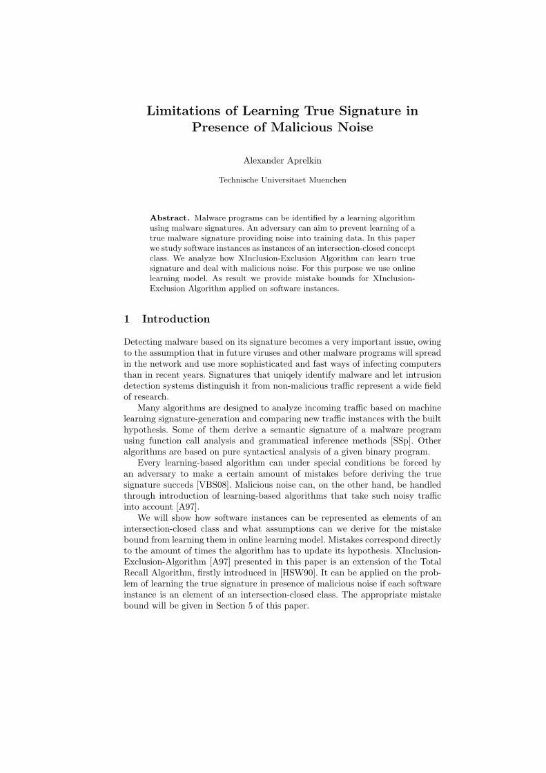
Example 2. For example, nested rectangles is a well known intersection-closedconcept class, which can be easily imagined by people.Each odd (black) nested rectangle from the outside can represent positive la-

Fig. 1. Intersection-closed concept class of nested rectangles

beled instances, each even (white) - the set of negative labeled instances.C =< C1, ..., C4 >= C1\(C2\(C3\C4)) = {Two black filled polygons}. This setcontains only positive examples in a noise-free case.

Definition 6. A linear space is an algebraical object, which consists of a setand two operations, addition and multiplication, with certain properties. A de-tailed definition is provided in [R2000].

An example of a linear space is the space {0, 1}m, m ∈ N. It has space dimension

m. [R2000]

We write MB(A, C, N) for maximal number of mistakes, the algorithm A makes,until it succesfully learns a concept C ∈ C, while N examples are noisy. If thereis no noise, we write MB(A, C). [A97]

2.2 Signature model

2.2.1 General model of signature and reflecting sets Data and codelook nearly the same as byte sequences and are located in the same memoryaccording to the von Neumann model. So, exploits are possible that manipulatedata and code. Therefore, we have to concentrate on the possible maliciousprograms as byte sequences.

Let us consider the alphabet Σ, which can be Unicode or ASCII characters,for instance. A byte sequence over this alphabet is a subset P ⊂ Σ∗. We willrefer to elements from P as programs.

Definition 7. A signature is a function over a byte sequence, which decideswhether the given byte sequence is malicious or not, i.e. we define signatureas σ : P → {0, 1}, where 0 means that the program is Malicious and 1 Non-Malicious.

Signatures are used to uniquely identify malware and to distinguish it fromnon-malicious programs. Normally each signature algorithm or function analyzesthe code for some patterns for each of the interesting attributes, which thealgorithm assumes to exist in the malicious program.

Signatures can be very complex and range from simple syntactical matchingof byte patterns in the program to semantical analysis of what program possiblyattempts to do, for example, what system calls can be made and what variablescan be influenced. Semantic signatures are considered to be less vulnerable thanthe syntactic, because the first ones are resistent against minor binary changesin the program.

Definition 8. We define attributes as boolean functions P → {0, 1} and con-sider signatures as conjunctions over the attributes.

If all attributes evaluate to true, the signature also evaluates to true. Thisconcludes that attributes define which byte sequences or other properties have tobe present or to be hold in the true signature and not which have to be absent.We define instances of software as it was done in [VBS08].

Definition 9. A software instance is a m-tuple i ∈ {0, 1}m, where m is the

total number of all possible attributes. The i-th 0 or 1 defines, whether the i-thattribute is present in the software instance. The instance space is defined asI = {i ∈ {0, 1}m}. If the set of attributes G is fixed and finite, so an m exists.

We define labels of the instances the following way: an example is labeledpositive, if it is malicious and negative if not. A hypothesis function classifiesan instance of being labeled positive or negative. False positive predictionerror means that a non-malicious instance is classiied as malicious one. Falsenegative means that a malicious instance is classified to be non-malicious.

Definition 10. A signature function is called a true signature if it achieves0 false positives and 0 false negatives.

Example 3. Let us consider the following example of a syntactical signature:let the attribute set G be {att1, att2, att3, att4, att5}, where the attributes aredefined as: att1=”x00”, att2=”xFE \ xA9”, att3=”xFF \ xFF”, att4=”xFF\ xAE”, att5=”xAA \ x01”. Let the true signature function be σ(p) = {1 ifatt1 ∧ att2 ∧ att3 = true and 0 otherwise}, what means that all attributes haveto be present in a byte sequence in order to let this byte sequence be evaluated asmalicious. An instance p1 could be for example (0, 1, 1, 1, 0), which means thatin p1 att1, att5 are not present, but att2, att3 and att4 are present. Therefore,p1 is a non-malicious program, as the conjunction over the attributes att1, att2and att3 evaluates to false.

In contrast, instance p2 = (1, 1, 1, 0, 1) would be evaluated as a maliciousone.

The true signature function corresponds to the target concept function inthe learning theory. True signature evaluates to true on those instances, whichare elements of the target concept. Attributes in the true signature are calledcritical attributes. All of these attributes must evaluate to true in maliciousinstances.

Some of critical attributes can be very expensive to identify, owing to theirequal likelihood of occurence with other attributes. A set of such similar at-tributes is referred to as the reflecting set of a given critical attribute. Thefollowing definition of reflecting set is taken from [VBS08].

Definition 11. Let PrA[S′] be the probability of a function S′ to be a true signa-ture in the output of learning algorithm A. Let C1, .., Cj denote sets of attributes,such that a critical attribute sr is contained in one of sets Cr ∈ {C1, ..., Cj}. Eachof elements in the set Cr can replace sr in the true signature.

Functions obtained through replacing critical attributes si with attributes fromsets C1, .., Cj that way build the set T . Suppose Wm is the set of maliciousinstances and Wnm the set of non-malicious instances that the algorithm A hasalready seen. W = Wm

⋃Wnm is the set of all seen instances.

Tw will represent the set of functions in T that classify the set W the rightway, i.e. functions that correctly distinguish between malious and non-maliciousinstances.

The sets C1, .., Cj are reflecting sets for a signature function S ∈ Tw andthe algorithm A, if for all pairs of true signature candidate functions T, T ′ ∈ Tw

for all sets W , PrA[T ] = PrA[T ′].

Example 4. Suppose that the true signature is ”xFE” ∧ ”xA9”. Critical at-tributes of this signature are ”xFE” and ”xA9”. A learning algorithm has alreadyseen some instances.

It now has built a hypothesis ”xFE” ∧ ”xA9”, but is unsure, if it could bethe unique true signature, because ”xFE” ∧ ”x0E”, ”xA2” ∧ ”xA9” and ”xA2”∧ ”x0E” also appear to be correct hypothesis.

So, the set Tw contains ”xFE” ∧ ”xA9”, ”xFE” ∧ ”x0E”, ”xA2” ∧ ”xA9”,”xA2” ∧ ”x0E”, the set of potential signatures.

One can see, that the set {”xFE”, ”xA2”} is a reflecting set for ”xFE” andthe set {”xA9”, ”x0E”} is the reflecting set for ”xA9”, because for all pairs offunctions T, T ′ ∈ Tw, the probability of being a true signature is equal.

Indeed,

• Pr[”xFE” ∧ ”xA9”] = Pr [”xFE” ∧ ”x0E”], because ”xA9” as well as ”x0E”can be replaced by ”x0E” or ”xA9” respectively in the true signature.

• Pr[”xFE” ∧ ”xA9”] = Pr [”xA2” ∧ ”xA9”],• Pr[”xFE” ∧ ”xA9”] = Pr [”xA2” ∧ ”x0E”],• Pr[”xFE” ∧ ”x0E”] = Pr [”xA2” ∧ ”xA9”],• Pr[”xFE” ∧ ”x0E”] = Pr [”xA2” ∧ ”x0E”] and• Pr[”xA2” ∧ ”xA9”] = Pr [”xA2” ∧ ”x0E”] with the same argumentation.

So, the algorithm has no possibility to distinguish between candidate truesignature function S to be the true signature and another candidate true signa-ture function S1, if each of their critical attributes is chosen from the respectivelysame reflection sets.

We assume that the adversary can manipulate and exploit the inability of learn-ing algorithm to distinguish between the attributes in a reflecting set. Thereforethe adversary would try to introduce such traffic, that forces the learning algo-rithm to learn a false signature, whose attributes are from the reflecting sets ofthe critical attributes of the true signature.

We furthermore assume, that an attacker can construct or find reflecting setsfor each of critical attributes. [VBS08]

2.2.2 Semantic signature The use of a semantic signature is very powerfulin detecting malware. We now show, how a semantic signature can be derived.

In [SSp] an inductive inference algorithm of constructing a true signature fordifferent types of attacks is provided. Using a disassembler a binary program isconverted into a graph of control flow and data dependence. This graph is thendivided into subgraphs and subblocks. Each of these subblocks contains a groupof sequentially called functions in the considered program which appear to leadto the same semantical security goal.

Definition 12. Abstract finite state transducer is a 6-tuple (Σ,Q, q, F, Γ, δ),where Σ is a finite set of input symbols, Q is a finite set of states, q ∈ Q isthe initial state, F ⊆ Q is a finite set of final states, Γ is a finite set of outputsymbols and δ is a transition function δ : Q × Σ → Q × Γ .

After the combination procedure, a conversion to abstract finite state trans-ducer takes place. Each subblock corresponds to one state of the transducer.

Two syntanctically different programs with same security vulnerabilities wouldresult in a same transducer.

Input symbols of the transducer are numbers of group of functions and outputsymbols are arguments to the group of functions. Final states of the transducercorrespond to subblocks which security goal is accomplished in or which pro-gram terminates in. Transducer can accept and reject strings using final states.Strings can be built as a concatenation of input and output symbols of eachtransition along the way from the initial state q to a final state. We define ourabstract finite state transducer to accept those strings which are built along theway from the initial state until an accepting state. Other strings will be rejected.

As in the transducer model the position of each state is important, a signatureargument has to contain the input symbol, the output symbol, and the numberrepresenting the depth of the state in the tranducer. The position of an input-output-token in a resulting string can be defined by this number.

Example 5. Groups of functions and arguments can be associated with numbersas follows:

1 Open file2 Write to file3 Read from file4 Exit5 Create a new process...33 Kill a process...

1 One argument, a string2 One argument, an integer greater than 1003 Two arguments, an integer greater than 100 and a string4 One argument, a string with length greater than 256...512 One argument, a string with length 5...

Attributes can be represented as a subset J ⊂ N×N×N, where the first numberrepresents input, the second output, the third the depth of state in transducer,i.e. the position in the string. This set is countable and has cardinality m.

A list of such attributes gives us again same representation as for generalsignature. True signature can then be defined as an element of space {0, 1}m

.An i-th one is set, if the correspondent i-th argument is present in the truesignature.

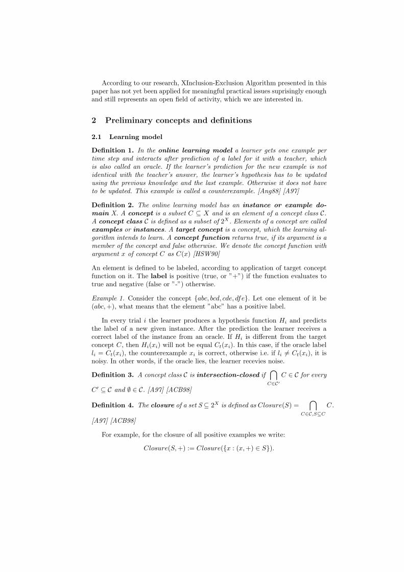
For instance, an j-th attribute in set G of attributes could be a 3-tuple(3, 512, 2). This combination means that the function group number 3 is calledand executed with security arguments 512, and it occured at the second position

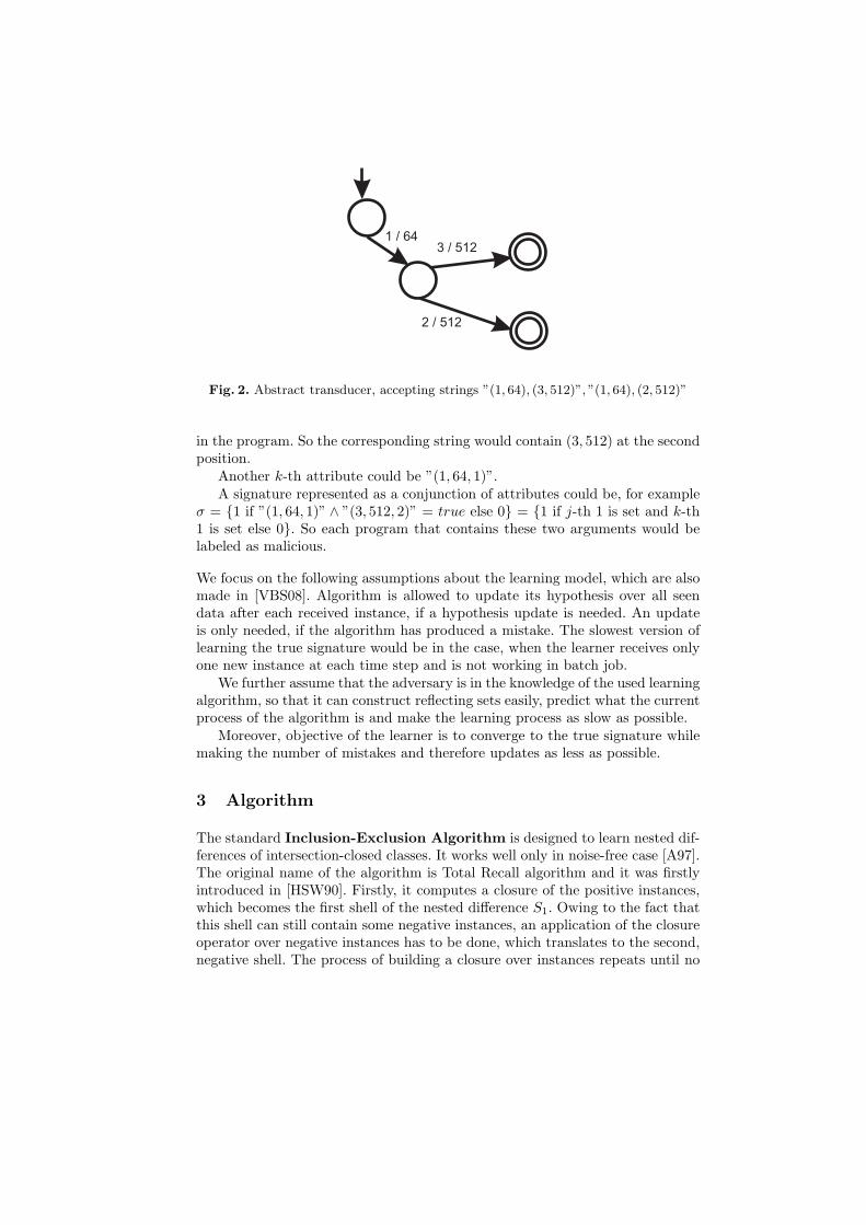
1 / 643 / 512

2 / 512

Fig. 2. Abstract transducer, accepting strings ”(1, 64), (3, 512)”, ”(1, 64), (2, 512)”

in the program. So the corresponding string would contain (3, 512) at the secondposition.

Another k-th attribute could be ”(1, 64, 1)”.A signature represented as a conjunction of attributes could be, for example

σ = {1 if ”(1, 64, 1)” ∧ ”(3, 512, 2)” = true else 0} = {1 if j-th 1 is set and k-th1 is set else 0}. So each program that contains these two arguments would belabeled as malicious.

We focus on the following assumptions about the learning model, which are alsomade in [VBS08]. Algorithm is allowed to update its hypothesis over all seendata after each received instance, if a hypothesis update is needed. An updateis only needed, if the algorithm has produced a mistake. The slowest version oflearning the true signature would be in the case, when the learner receives onlyone new instance at each time step and is not working in batch job.

We further assume that the adversary is in the knowledge of the used learningalgorithm, so that it can construct reflecting sets easily, predict what the currentprocess of the algorithm is and make the learning process as slow as possible.

Moreover, objective of the learner is to converge to the true signature whilemaking the number of mistakes and therefore updates as less as possible.

3 Algorithm

The standard Inclusion-Exclusion Algorithm is designed to learn nested dif-ferences of intersection-closed classes. It works well only in noise-free case [A97].The original name of the algorithm is Total Recall algorithm and it was firstlyintroduced in [HSW90]. Firstly, it computes a closure of the positive instances,which becomes the first shell of the nested difference S1. Owing to the fact thatthis shell can still contain some negative instances, an application of the closureoperator over negative instances has to be done, which translates to the second,negative shell. The process of building a closure over instances repeats until no

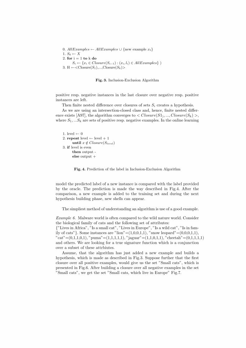
0. AllExamples← AllExamples ∪ {new example xt}1. S0 ← X2. for i = 1 to k do

Si ← {xi ∈ Closure(Si−1) : (xi, li) ∈ AllExamples} )3. H ←<Closure(S1),...,Closure(Sk)>

Fig. 3. Inclusion-Exclusion Algorithm

positive resp. negative instances in the last closure over negative resp. positiveinstances are left.

Then finite nested difference over closures of sets Si creates a hypothesis.

As we are using an intersection-closed class and, hence, finite nested differ-ence exists [A97], the algorithm converges to < Closure(S1), ..., Closure(Sk) >,where S1, ...Sk are sets of positive resp. negative examples. In the online learning

1. level ← 02. repeat level ← level + 1

until x /∈ Closure(Slevel)3. if level is even

then output -else output +

Fig. 4. Prediction of the label in Inclusion-Exclusion Algorithm

model the predicted label of a new instance is compared with the label providedby the oracle. The prediction is made the way described in Fig.4. After thecomparison, a new example is added to the training set and during the nexthypothesis building phase, new shells can appear.

The simpliest method of understanding an algorithm is use of a good example.

Example 6. Malware world is often compared to the wild nature world. Considerthe biological family of cats and the following set of attributes:{”Lives in Africa”, ”Is a small cat”, ”Lives in Europe”, ”Is a wild cat”, ”Is in fam-ily of cats”}. Some instances are ”lion”=(1,0,0,1,1), ”snow leopard”=(0,0,0,1,1),”cat”=(0,1,1,0,1), ”puma”=(1,1,1,1,1), ”jaguar”=(1,1,0,1,1), ”cheetah”=(0,1,1,1,1)and others. We are looking for a true signature function which is a conjunctionover a subset of these attrbiutes.

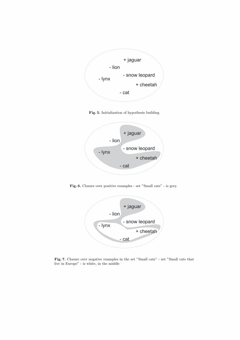
Assume, that the algorithm has just added a new example and builds ahypothesis, which is made as described in Fig.3. Suppose further that the firstclosure over all positive examples, would give us the set ”Small cats”, which ispresented in Fig.6. After building a closure over all negative examples in the set”Small cats”, we get the set ”Small cats, which live in Europe” Fig.7.

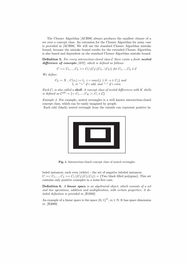
- lion

+ jaguar

- cat

- snow leopard- lynx

+ cheetah

Fig. 5. Initialization of hypothesis building

- lion

+ jaguar

- cat

- snow leopard- lynx

+ cheetah

Fig. 6. Closure over positive examples - set ”Small cats” - is grey.

- lion

+ jaguar

- cat

- snow leopard- lynx

+ cheetah

Fig. 7. Closure over negative examples in the set ”Small cats” - set ”Small cats thatlive in Europe” - is white, in the middle

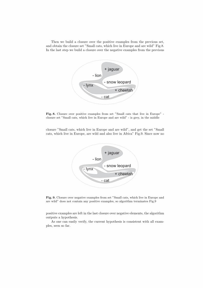
Then we build a closure over the positive examples from the previous set,and obtain the closure set ”Small cats, which live in Europe and are wild” Fig.8.In the last step we build a closure over the negative examples from the previous

- lion

+ jaguar

- cat

- snow leopard- lynx

+ cheetah

Fig. 8. Closure over positive examples from set ”Small cats that live in Europe” -closure set ”Small cats, which live in Europe and are wild” - is grey, in the middle

closure ”Small cats, which live in Europe and are wild”, and get the set ”Smallcats, which live in Europe, are wild and also live in Africa” Fig.9. Since now no

- lion

+ jaguar

- cat

- snow leopard- lynx

+ cheetah

Fig. 9. Closure over negative examples from set ”Small cats, which live in Europe andare wild” does not contain any positive examples, so algorithm terminates Fig.9

positive examples are left in the last closure over negative elements, the algorithmoutputs a hypothesis.

As one can easily verify, the current hypothesis is consistent with all exam-ples, seen so far.

Assume that now a new example ”puma” arrives. The prediction algorithmstarts from the level 0. Level is at the beginning incremented by one. Checkif puma is in the set ”Small cats” succeeds. Level goes to two. Now puma isalso in the set ”Small cats, which live in Europe”. Level increments and now isthree. Puma is in the set ”Small cats, which live in Europe and are wild” as well.Level goes to four. Now, as we assume that pumas do not live in Africa, example”puma” is not in the current hypothesis set that is ”Small cats, which live inEurope, Africa and are wild”, therefore the prediction terminates and outputs”+”, since current level four is an even number.

After that, the oracle provides the real label to the example ”puma”, whichcan be either ”+” or ”-”. A new hypothesis function is then built the way asdescribed above even if the label was predicted correctly.

- lion+ jaguar

- cat

- snow leopard- lynx

+ cheetah

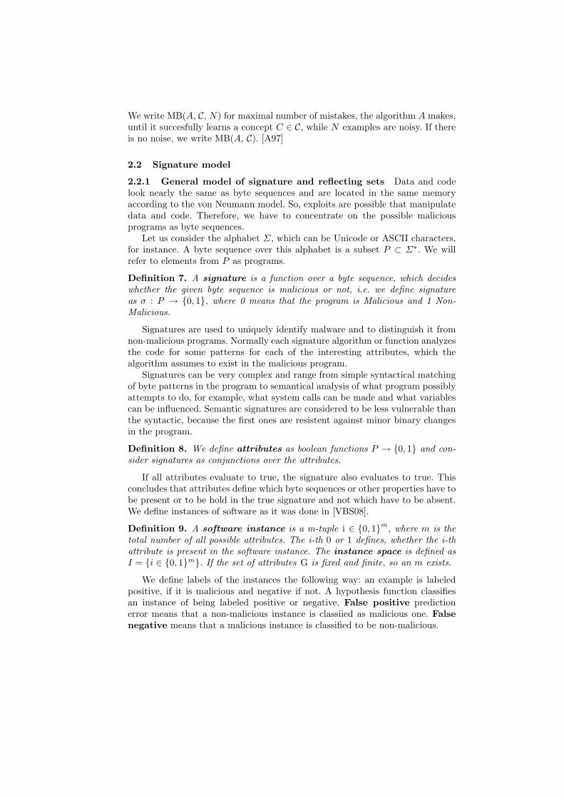
- leopard

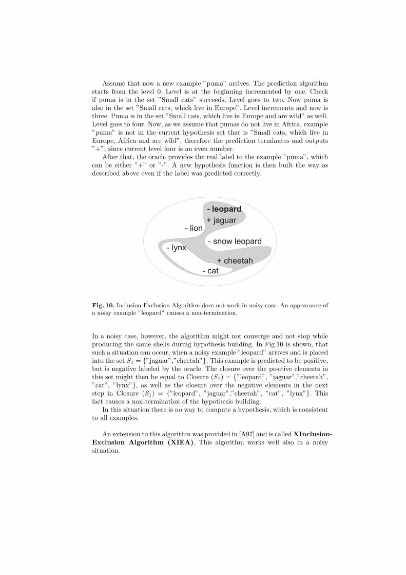
Fig. 10. Inclusion-Exclusion Algorithm does not work in noisy case. An appearance ofa noisy example ”leopard” causes a non-termination.

In a noisy case, however, the algorithm might not converge and not stop whileproducing the same shells during hypothesis building. In Fig.10 is shown, thatsuch a situation can occur, when a noisy example ”leopard” arrives and is placedinto the set S1 = {”jaguar”,”cheetah”}. This example is predicted to be positive,but is negative labeled by the oracle. The closure over the positive elements inthis set might then be equal to Closure (S1) = {”leopard”, ”jaguar”,”cheetah”,”cat”, ”lynx”}, as well as the closure over the negative elements in the nextstep in Closure (S1) = {”leopard”, ”jaguar”,”cheetah”, ”cat”, ”lynx”}. Thisfact causes a non-termination of the hypothesis building.

In this situation there is no way to compute a hypothesis, which is consistentto all examples.

An extension to this algorithm was provided in [A97] and is called XInclusion-Exclusion Algorithm (XIEA). This algorithm works well also in a noisysituation.

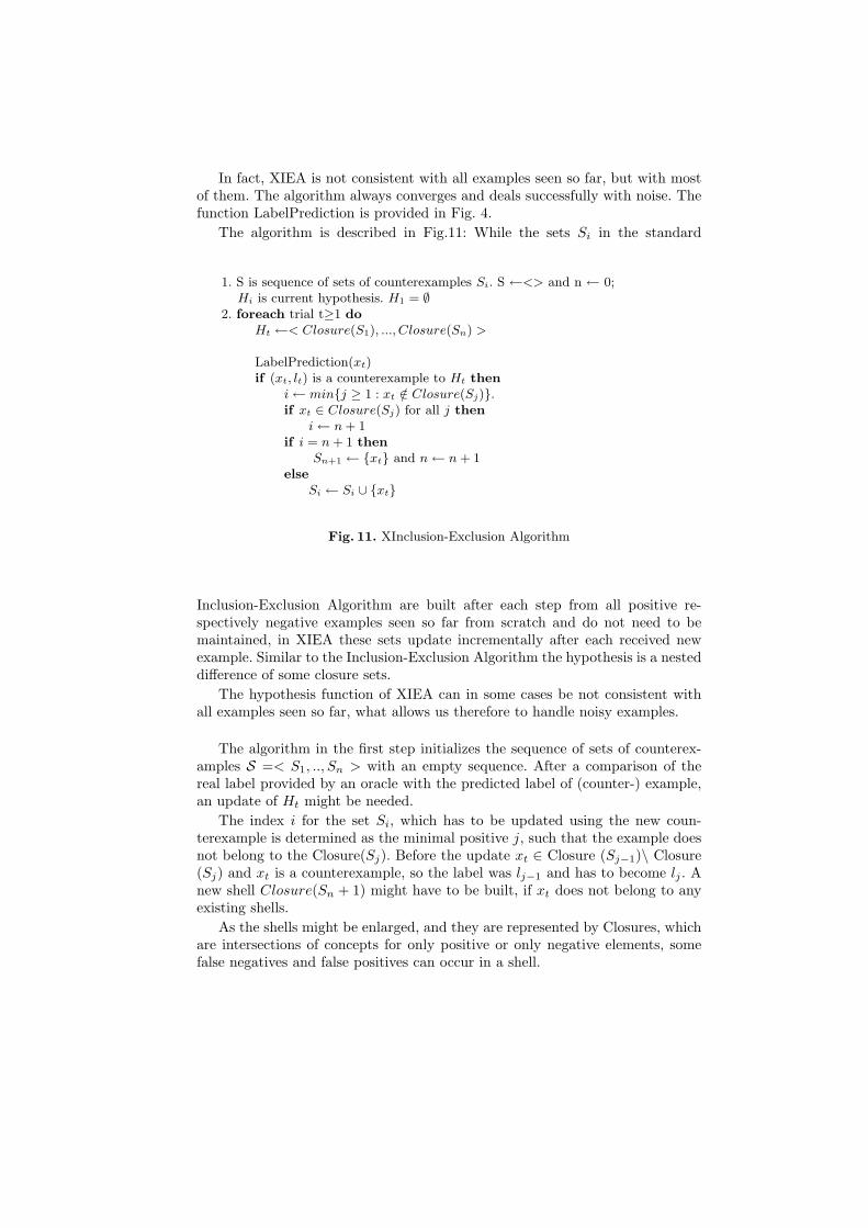
In fact, XIEA is not consistent with all examples seen so far, but with mostof them. The algorithm always converges and deals successfully with noise. Thefunction LabelPrediction is provided in Fig. 4.

The algorithm is described in Fig.11: While the sets Si in the standard

1. S is sequence of sets of counterexamples Si. S ←<> and n ← 0;Hi is current hypothesis. H1 = ∅

2. foreach trial t≥1 do

Ht ←< Closure(S1), ..., Closure(Sn) >

LabelPrediction(xt)if (xt, lt) is a counterexample to Ht then

i← min{j ≥ 1 : xt /∈ Closure(Sj)}.if xt ∈ Closure(Sj) for all j then

i← n + 1if i = n + 1 then

Sn+1 ← {xt} and n← n + 1else

Si ← Si ∪ {xt}

Fig. 11. XInclusion-Exclusion Algorithm

Inclusion-Exclusion Algorithm are built after each step from all positive re-spectively negative examples seen so far from scratch and do not need to bemaintained, in XIEA these sets update incrementally after each received newexample. Similar to the Inclusion-Exclusion Algorithm the hypothesis is a nesteddifference of some closure sets.

The hypothesis function of XIEA can in some cases be not consistent withall examples seen so far, what allows us therefore to handle noisy examples.

The algorithm in the first step initializes the sequence of sets of counterex-amples S =< S1, .., Sn > with an empty sequence. After a comparison of thereal label provided by an oracle with the predicted label of (counter-) example,an update of Ht might be needed.

The index i for the set Si, which has to be updated using the new coun-terexample is determined as the minimal positive j, such that the example doesnot belong to the Closure(Sj). Before the update xt ∈ Closure (Sj−1)\ Closure(Sj) and xt is a counterexample, so the label was lj−1 and has to become lj . Anew shell Closure(Sn + 1) might have to be built, if xt does not belong to anyexisting shells.

As the shells might be enlarged, and they are represented by Closures, whichare intersections of concepts for only positive or only negative elements, somefalse negatives and false positives can occur in a shell.

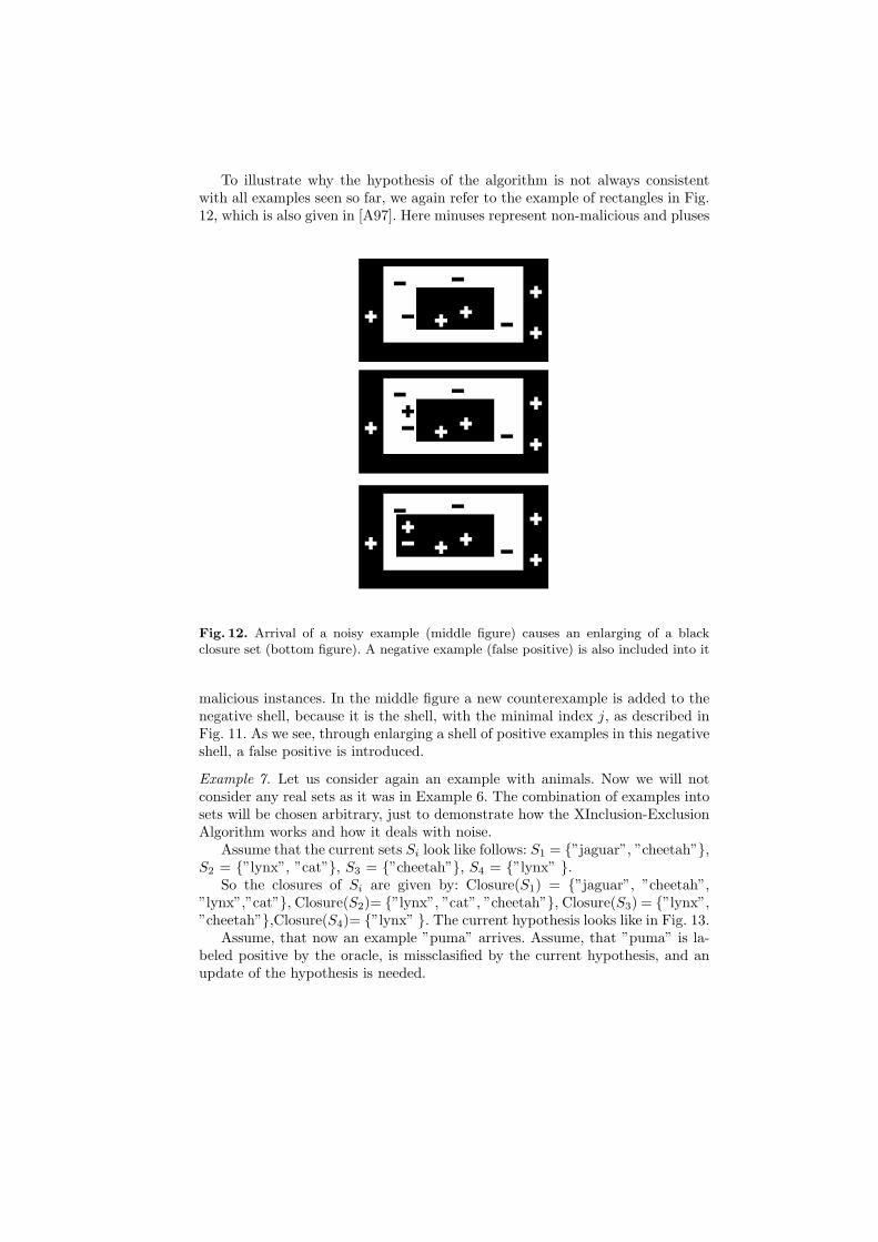
To illustrate why the hypothesis of the algorithm is not always consistentwith all examples seen so far, we again refer to the example of rectangles in Fig.12, which is also given in [A97]. Here minuses represent non-malicious and pluses

Fig. 12. Arrival of a noisy example (middle figure) causes an enlarging of a blackclosure set (bottom figure). A negative example (false positive) is also included into it

malicious instances. In the middle figure a new counterexample is added to thenegative shell, because it is the shell, with the minimal index j, as described inFig. 11. As we see, through enlarging a shell of positive examples in this negativeshell, a false positive is introduced.

Example 7. Let us consider again an example with animals. Now we will notconsider any real sets as it was in Example 6. The combination of examples intosets will be chosen arbitrary, just to demonstrate how the XInclusion-ExclusionAlgorithm works and how it deals with noise.

Assume that the current sets Si look like follows: S1 = {”jaguar”, ”cheetah”},S2 = {”lynx”, ”cat”}, S3 = {”cheetah”}, S4 = {”lynx” }.

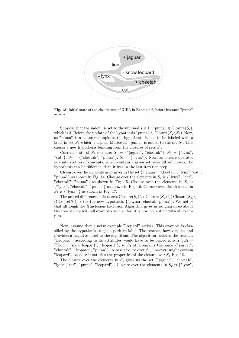
So the closures of Si are given by: Closure(S1) = {”jaguar”, ”cheetah”,”lynx”,”cat”}, Closure(S2)= {”lynx”, ”cat”, ”cheetah”}, Closure(S3) = {”lynx”,”cheetah”},Closure(S4)= {”lynx” }. The current hypothesis looks like in Fig. 13.

Assume, that now an example ”puma” arrives. Assume, that ”puma” is la-beled positive by the oracle, is missclasified by the current hypothesis, and anupdate of the hypothesis is needed.

- lion

+ jaguar

- cat

- snow leopard- lynx

+ cheetah

Fig. 13. Initial state of the closure sets of XIEA in Example 7, before instance ”puma”arrives

Suppose that the index i is set to the minimal j ≥ 1 : ”puma” /∈ Closure(Sj),which is 3. Before the update of the hypothesis ”puma” ∈ Closure(S2\S3). Now,as ”puma” is a counterexample to the hypothesis, it has to be labeled with alabel in set S3 which is a plus. Moreover, ”puma” is added to the set S3. Thiscauses a new hypothesis building from the closures of sets Si.

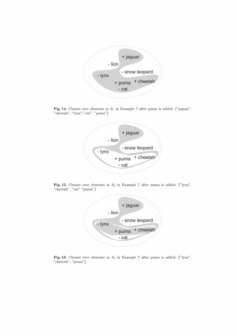
Current state of Si sets are: S1 = {”jaguar”, ”cheetah”}, S2 = {”lynx”,”cat”}, S3 = {”cheetah”, ”puma”}, S4 = {”lynx”}. Now, as closure operatoris a intersection of concepts, which contain a given set, over all subclasses, thehypothesis can be different, than it was in the last iteration step.

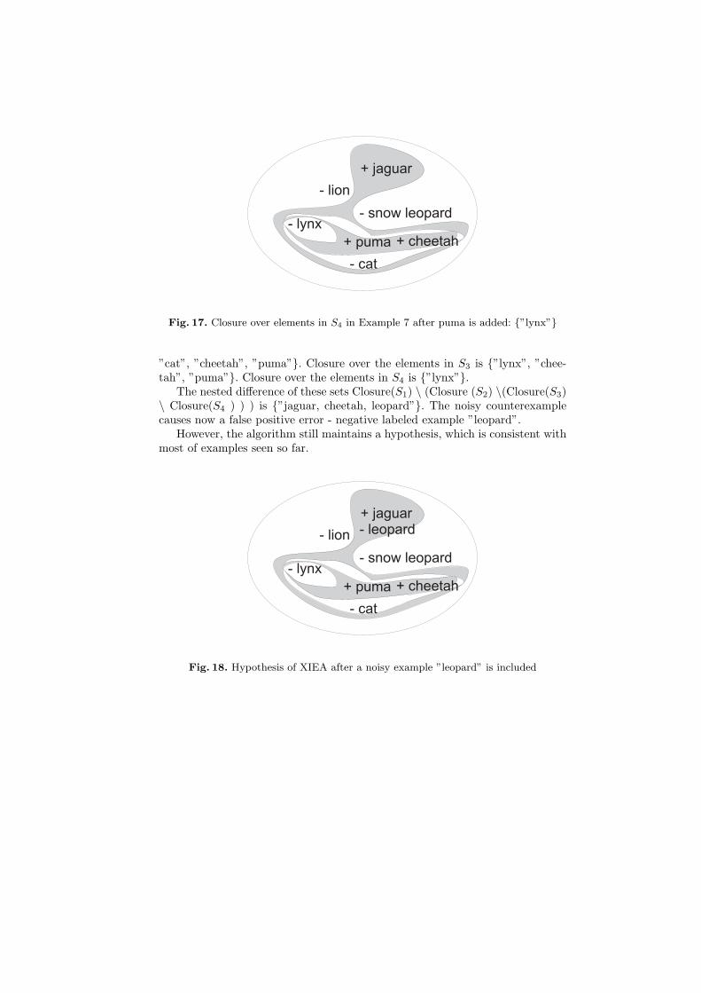
Closure over the elements in S1 gives us the set {”jaguar”, ”cheetah”, ”lynx”,”cat”,”puma”} as shown in Fig. 14. Closure over the elements in S2 is {”lynx”, ”cat”,”cheetah”, ”puma”} as shown in Fig. 15. Closure over the elements in S3 is{”lynx”, ”cheetah”, ”puma”} as shown in Fig. 16. Closure over the elements inS4 is {”lynx” } as shown in Fig. 17.

The nested difference of these sets Closure(S1) \ ( Closure (S2) \ ( Closure(S3)\(Closure(S4)) ) ) is the new hypothesis {”jaguar, cheetah, puma”}. We noticethat although the XInclusion-Exclusion Algorithm gives us no guarantee aboutthe consistency with all examples seen so far, it is now consistent with all exam-ples.

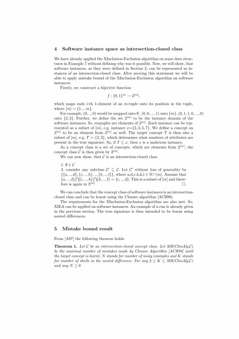
Now, assume that a noisy example ”leopard” arrives. This example is clas-sified by the hypothesis to get a positive label. The teacher, however, lies andprovides a negative label to the algorithm. The algorithm believes the teacher.”Leopard”, according to its attributes would have to be placed into X \ S1 ={”lion”, ”snow leopard”, ”leopard”}, so S1 still remains the same {”jaguar”,”cheetah”, ”leopard”, ”puma”}. A new closure over S1, however, might contain”leopard”, because it satisfies the properties of the closure over S1 Fig. 18.

The closure over the elements in S1 gives us the set {”jaguar”, ”cheetah”,”lynx”,”cat”, ”puma”, ”leopard”}. Closure over the elements in S2 is {”lynx”,

- lion

+ jaguar

- cat

- snow leopard- lynx

+ cheetah+ puma

Fig. 14. Closure over elements in S1 in Example 7 after puma is added: {”jaguar”,”cheetah”, ”lynx”,”cat”, ”puma”}.

- lion

+ jaguar

- cat

- snow leopard- lynx

+ cheetah+ puma

Fig. 15. Closure over elements in S2 in Example 7 after puma is added: {”lynx”,”cheetah”, ”cat” ”puma”}

- lion

+ jaguar

- cat

- snow leopard- lynx

+ cheetah+ puma

Fig. 16. Closure over elements in S3 in Example 7 after puma is added: {”lynx”,”cheetah”, ”puma”}

- lion

+ jaguar

- cat

- snow leopard- lynx

+ cheetah+ puma

Fig. 17. Closure over elements in S4 in Example 7 after puma is added: {”lynx”}

”cat”, ”cheetah”, ”puma”}. Closure over the elements in S3 is {”lynx”, ”chee-tah”, ”puma”}. Closure over the elements in S4 is {”lynx”}.

The nested difference of these sets Closure(S1) \ (Closure (S2) \(Closure(S3)\ Closure(S4 ) ) ) is {”jaguar, cheetah, leopard”}. The noisy counterexamplecauses now a false positive error - negative labeled example ”leopard”.

However, the algorithm still maintains a hypothesis, which is consistent withmost of examples seen so far.

- lion

+ jaguar

- cat

- snow leopard- lynx

+ cheetah+ puma

- leopard

Fig. 18. Hypothesis of XIEA after a noisy example ”leopard” is included

4 Software instance space as intersection-closed class

We have already applied the XInclusion-Exclusion algorithm on some data struc-tures in Example 7 without defining why was it possible. Now, we will show, thatsoftware instances, as they were defined in Section 2, can be represented as in-stances of an intersection-closed class. After proving this statement we will beable to apply mistake bound of the XInclusion-Exclusion algorithm on softwareinstances.

Firstly, we construct a bijective function

f : {0, 1}m → 2[m],

which maps each i-th 1-element of an m-tuple onto its position in the tuple,where [m] = {1, ...m}.

For example, (0, .., 0) would be mapped onto ∅ , (0, 0, ..., 1) onto {m}, (0, 1, 1, 0, ..., 0)onto {2, 3}. Further, we define the set 2[m] to be the instance domain of thesoftware instances. So, examples are elements of 2[m]. Each instance can be rep-resented as a subset of [m], e.g. instance x={2, 3, 5, 7}. We define a concept on2[m] to be an element from 2[m] as well. The target concept T is then also asubset of [m], e.g. T = {2, 3}, which determines what numbers of attributes arepresent in the true signature. So, if T ⊆ x, then x is a malicious instance.

As a concept class is a set of concepts, which are elements from 2[m], theconcept class C is then given by 2[m].

We can now show, that C is an intersection-closed class.

1. ∅ ∈ C2. consider any subclass C′ ⊆ C. Let C′ without loss of generality be{{a, .., d}, {c, .., h}, .., {k, .., l}}, where a,d,c,h,k,l ∈ N∩ [m]. Assume that{a, .., d}

⋂{c, .., h}

⋂{k, .., l} = {c, .., d}. This is a subset of [m] and there-

fore is again in 2[m]�.

We can conclude that the concept class of software instances is an intersection-closed class and can be learnt using the Closure algorithm [ACB98].

The requirements for the XInclusion-Exclusion algorithm are also met. So,XIEA can be applied on software instances. An example of a run is already givenin the previous section. The true signature is then intended to be learnt usingnested differences.

5 Mistake bound result

From [A97] the following theorem holds:

Theorem 1. Let C be an intersection-closed concept class. Let MB(ClosAlg,C)be the maximal number of mistakes made by Closure Algorithm [ACB98] untilthe target concept is learnt. N stands for number of noisy examples and K standsfor number of shells in the nested difference. For any 2 ≤ K ≤ MB(ClosAlg,C)and any N ≥ 0

MB(XInclusionExclusionAlg, C(K), N) ≤ (2N + K)MB(ClosAlg, C) - K(K−1)2

A proof is given in [A97]. As mentioned in [ACB98], if C is a set of allsubspaces of a d-dimensional linear space, then MB(ClosAlg, C) = d. In ourcase, {0, 1}m

is a linear space with dimension m, as stated above in Section2. It has only two subspaces, the smallest linear space, vector {0}m

and itself.Thus, the correspondent concept class C = 2[m] contains all subspaces of {0, 1}m

.Therefore, MB(ClosAlg, C) = m.

Theorem 2. Let A be a deterministic signature learning algorithm. An adver-sary can introduce a sequence of instances into training data, such that A isforced make at least n log k mistakes, where k is the size of reflecting sets and nis the number of bits in the true signature which evaluate to true.

This theorem is proven for the noise-free case in [VBS08].Now, we can combine the results from above theorems and construct a state-

ment for mistake bounds of XInclusion-Exclusion Algorithm, which contains theproperties of malware signature.

Since XInclusion-Exclusion Algorithm is a deterministic algorithm, the resultof Theorem 2 holds in a noise-free case, which means:

n log k ≤ MB(XInclusionExclusionAlg, C(K)).

If noise is allowed, the lower mistake bound of XInclusion-Exclusion Algorithmcan be even greater and especially

n log k ≤ MB(XInclusionExclusionAlg, C(K), N).

On the other hand, using the Theorem 1,

MB(XInclusionExclusion, C(K),N) ≤ (2N + K) MB(ClosAlg,C) - K(K−1)2 .

Substituting the dimension m into the last equation gives:

MB(XInclusionExclusion, C(K),N) ≤ (2N + K)m) - K(K−1)2 )

K represents the number of nested differences, therefore there could be at least Kattributes set to 1 in the target concept, so that each of them can be distinguishedfrom another in the way that each of them can be maximally in a separate shell.So

K ≤ n,

where n is number of attributes in the true signature which have to evaluate totrue.

As K can only be between 2 and MB(ClosAlg,C) according to the condi-tions of Theorem 2, we assume that the number of attributes n is bounded byMB(ClosAlg, C) from above to apply Theorem 1. So,

n ≤ MB(ClosAlg,C)

and

K ≤ MB(ClosAlg,C)

Using these inequalities we can state,

(2N + K) MB(ClosAlg,C) - K(K−1)2 ≤ (2N + MB(ClosAlg,C))MB(ClosAlg,C) -

n(n−1)2 .

The equality holds if number of attributes in the target concept equalsMB(ClosAlg,C) and each attribute corresponds to a separate shell.

Again, substituting m into the last inequality and using the results of Theo-rem 1 and Theorem 2 gives:

n log k ≤ MB(XInclusionExclusion, C(K),N) ≤ (2N + m)m - n(n−1)2 .

So we have obtained a mistake bound for the XInclusion-Exclusion Algorithm,which is dependent on the properties of signatures: number n of attributes thatevaluate to true in the true signature, size of reflection sets k and total numberof attributes m.

6 Conclusion

We analyzed the learnability of the true signature and software instances asinstances of an intersection-closed concept class. For this purpose we used theXInclusion-Exclusion Algorithm in the online learning model and have shownthat the algorithm can be applied on software instances. We also focused on themistake bounds for this algorithm dependent on properties of software instancesin presence of malicious noise.

References

[A97] P. Auer. Learning Nested Differences in the Presence of Malicious Noise. The-oretical Computer Science 185(1):159-175, Elsevier Science Publishers Ltd, Essex,UK, 1997

[ACB98] P. Auer, N. Cesa-Bianchi. On-line learning with malicious noise and the clo-sure algorithm. Annals of Mathematics and Artificial Intelligence 23(83-99), KluwerAcademic Publishers, Hingham, MA, USA, 1998

[VBS08] S. Venkataraman, A. Blum, D. Song. Limits of Learning-based Signature Gen-eration with Adversaries. In Proceedings of the 15th Annual Network & DistributedSystem Security Symposium, 2008

[HSW90] D. Helmbold, R. Sloan, M.K.Warmuth. Learning Nested Differences ofInteresection-Closed Classes. Machine Learning 5:165-196, Kluwer Academic Pub-lishers, Boston, 1990

[SSp] J. Shin, D. F. Spears. The Basic Building Blocks of Malware. Machine Learning5:165-196, University of Wyoming, Laramie.

[Ang88] D. Angluin. Queries and concept learning. Machine Learning. 2(4):314-342,April 1988.

[R2000] K. Rosen. Handbook of discrete and combinatorial mathematics. CRC Press,USA, 2000.