Semiparametric Estimation of Lifetime Equivalence Scales

Krishna Pendakur

Department of Economics

Simon Fraser University

Burnaby, BC, CANADA, V5A 1S6 pendakur@sfu.ca

Received: ; Accepted:

Abstract

Pashardes (1991) and Banks, Blundell and Preston (1994) use parametric methods

to estimate lifetime equivalence scales. Their approaches put parametric restrictions on

the differences in within-period expenditure needs across household types, the intertem-

poral allocation of expenditure, and the shapes of commodity demand equations. This

paper puts parametric structure only on the differences in within-period expenditure

needs across household types. This implies structure on the intertemporal allocation of

expenditure, but leaves the shapes of commodity demand equations unrestricted. Semi-

parametric methods are used to estimate within-period and lifetime equivalence scales

with Canadian expenditure data, and to test the restrictions imposed on within-period

expenditure functions. Estimated lifetime equivalence scales are similar in size to those

estimated by Banks, Blundell and Preston, and exhibit equal lifetime costs for first and

second children.

JEL classification: C14; C43; D11; D12; D63

Keywords: Equivalence scales; Semiparametric estimation; Consumer demand

_________

I acknowledge the financial support of the Social Sciences and Humanities Research

Council of Canada through its Equality, Security and Community research initiative. I

am grateful for the comments of two anonymous referees and for the ideas and encourage-

ment of my colleagues: Doug Allen, Richard Blundell, Tom Crossley, David Donaldson,

Panayiota Lyssioutou, Federico Perali, Joris Pinkse, Ian Preston, Thanassis Stengos, and

John Wald. Of course, any errors that remain are my own.

1

1. Introduction

Equivalence scales that evaluate differences in expenditure needs across household types

are of great empirical and policy interest, but are difficult to measure. Although under

certain circumstances demand analysis can reveal within-period equivalence scales, the real

object of interest is lifetime equivalence scales which reveal differences in lifetime expenditure

needs across household types. To the extent that households can save and borrow to move

expenditure across periods, within-period equivalence scales may be a poor indicator of

lifetime differences in expenditure needs.

Since an agent’s solution to the intertemporal allocation problem may result in within-

period utility levels that are different over time, lifetime utility may be more appropriate

than within-period utility as a measure of well-being from the policy point of view. If tax-

transfer systems seek to redistribute in order to achieve a more equal distribution of lifetime

utility, then lifetime equivalence scales may be more useful to policy-makers than within-

period equivalence scales. In addition, the use of lifetime equivalence scale allows the policy

maker to drop the age of children (and adults) from equivalence scales because households

are left to solve the intertemporal problem themselves.

Pashardes (1991) and Banks, Blundell and Preston (1994) use parametric methods to

estimate lifetime equivalence scales. Their approaches put parametric restrictions on the

differences in within-period expenditure needs across household types, the intertemporal al-

location of expenditure, and the shapes of within-period commodity demand equations. This

paper puts parametric structure only on the differences in within-period expenditure needs

across household types. This implies structure on the intertemporal allocation of expen-

diture, but leaves the shapes of within-period commodity demand equations unrestricted.

2

Semiparametric methods are used to estimate within-period and lifetime equivalence scales

with Canadian expenditure data.

This paper investigates the lifetime equivalence scales that result if within-period absolute

equivalence scales are exact. The absolute equivalence scale is the dollar amount necessary

to compensate a household for the presence of children or other household characteristics1 .

An absolute equivalence scale is exact if and only if it is the same at every utility level.

Under certain conditions, if the within-period absolute equivalence scale is exact, then the

lifetime absolute equivalence scale must also be exact, and is equal to the present discounted

value of all the within-period absolute equivalence scales in each period of the household’s life.

Further, if within-period absolute equivalence scales are exact, then household commodity

demand equations must have the same shape across household types. However, no additional

restrictions are placed on the shapes of household commodity demand equations. Thus, the

estimation of exact absolute equivalence scales is amenable to semiparametric methods.

Using semiparametric methods developed in Blundell, Duncan and Pendakur (1998) and

Pendakur (1999) and Canadian expenditure data, within-period absolute equivalence scales

are estimated under the restriction that they are exact, and lifetime equivalence scales are

calculated. Since exactness of the equivalence scale implies semiparametric shape restrictions

on commodity demand equations, these restrictions are tested against a fully nonparametric

alternative, which provides a partial test of the model.

Although the maintained assumption that within-period absolute equivalence scales are

exact is a strong one, I am able to strengthen its plausibility in two ways. First, the observable

restrictions implied by the existence of exact absolute within-period equivalence scales are

tested against a fully nonparametric alternative. These restrictions are not rejected by the

data for many inter-household comparisons. Second, estimation is conducted on a sample

1 There is a large literature on ‘ratio’ equivalence scales, which give the ratio of expenditures across householdtypes. For a discussion of the relationship between absolute and relative equivalence scales, see Blackorbyand Donaldson (1994).

3

consisting of households whose heads have no post-secondary education. In comparison with

the entire population, this population subsample has lower mean income, lifetime wealth and

total expenditure, and lower variance in total expenditure. The assumption that child costs

do not vary with utility may be more plausible for this subsample.

Semiparametric estimates of lifetime equivalence scales suggest that, compared with the

reference childless couple household, the lifetime equivalence scale for couples with one and

two children is approximately $39,000 and $77,000 of real expenditure, respectively. These

lifetime scales amount to approximately 12% of lifetime real expenditure for each child for

the average childless couples.

2. Lifetime Expenditure Functions

Define pt = [pt1,...,ptM ]

0 as an M − vector of prices, zt = [zt1,...,ztL]0 as an L − vector of

demographic characteristics, and ut as utility, all indexed to time period t. The within-

period expenditure function e(pt, ut, zt) gives the total expenditure required for a household

with demographic characteristics zt facing prices pt to achieve utility level ut. Define a vector

of reference characteristics z = [z1,...,zL]0, and write the within-period expenditure function

for the reference household as e(pt, ut) = e(pt, ut, z).

Consider an agent2 with an intertemporally additive direct lifetime utility function in an

environment of perfect information and perfect credit markets (see Keen 1990 and Pashardes

1991). Define lifetime utility as U =PTt=1 β

tut where βt is the time preference discount from

period 1 to period t.3 Define ρt as the credit market discount from period 1 to period t. An

2 For this analysis, I assume that the agent is a finitely lived household, maximising a household welfarefunction. If the household welfare function is maximin over household member utilities, then ut gives theutility of each household member in time period t. Alternatively, we may interpret ut as the equally distributedequivalent utility for the household welfare function over household member utilities.3 The assumption that lifetime utility U is the discounted sum of within-period utility is important forthis application. If, for example, U = f(

PT

t=1βtut, Z), then solving for lifetime expenditures which hold

U constant while varying Z becomes intractable, even with the restrictions developed below. I thank ananonymous referee for noticing the importance of the form of lifetime utility.

4

agent will choose ut as follows:

minut

L =TXt=1

ρte(pt, ut, zt)− λ

ÃTXt=1

βtut −U!. (1)

The solution(s) to (1) are given by solving the first order conditions

∂e(pt, ut, zt)

∂u=

βt

ρtλ (2)

TXt=1

βtut = U.

These conditions require that agents equate the credit market and time preference dis-

counted marginal price of utility across periods. The dependence of the marginal price of

utility, ∂e(pt, ut, zt)/∂u, on utility and demographic characteristics in time t allows the agent

to get more lifetime utility by shifting expenditure towards periods where the marginal price

of utility is low.

Defining ut∗ as the set of utilities that satisfy the first order conditions (2), we can

write out the lifetime expenditure function using these solved values. Denoting the price

profile P = [p1; ...; pT ], the demographic profile, Z = [z1; ...; zT ] and a reference demographic

profile Z = [z1; ...; zT ], the lifetime expenditure function E(P,U,Z) is given by:

E(P,U,Z) =TXt=1

ρte(pt, ut∗, zt), (3)

and we write the lifetime reference expenditure function as E(P,U) = E(P,U,Z).

Define the absolute lifetime equivalence scale, D(P,U, Z), as the difference between life-

time expenditures for the reference household and a nonreference household:

D(P,U, Z) = E(P,U,Z)−E(P,U). (4)

To economise on terminology, the term lifetime scale will be used to refer to the absolute

lifetime equivalence scale. We say that lifetime scale is exact if and only if it is independent

of lifetime utility. In this case, we denote the exact lifetime scale as ∆(P,Z) = D(P,U,Z)

where D is independent of U .

5

Consider an information environment of ordinal noncomparability, where we can trans-

form utility arbitrarily by a function φ(ut, zt). Because φ is independent of prices, it has no

effect on within-period behaviour (see, eg, Pollak and Wales 1979). However, it does have an

effect on the intertemporal allocation of utility because it may affect the marginal price of

utility. It also has an effect on lifetime scales because it affects the cost of demographic char-

acteristics. Thus, to estimate lifetime scales, the function φ must be known, and it cannot

be estimated from within-period demand behaviour.

Pashardes (1991) measures lifetime scales4 by assuming that within-period expenditure

function is given by the Almost Ideal model. This solution imposes that the log of e is linear

in φ and that φ(ut, zt) = ut. Thus, the model restricts the log of expenditures to be linear

in utility, and restricts the unobservable function φ to be independent of z and equal to

utility. The former restriction implies that within-period expenditure share equations are

linear in the log of total expenditure, a functional form that has been shown to fit actual

expenditure data quite poorly (see, for example, Blundell, Pashardes and Guglielmo, 1993;

Banks, Blundell and Lewbel, 1997).

Banks, Blundell and Preston (1994) relax both of these restrictions used by Pashardes.

They use quasi-panel estimates of the intertemporal substitution elasticity, which identifies φ

up to a z-dependent linear transformation of u, and assume that within-period expenditure

share equations are quadratic in the log of total expenditure. Because φ is still only partially

identified, they further assume that the effects of zt on φ are such that the estimated lifetime

scales “are plausible”.

Three drawbacks to the approach of Banks, Blundell and Preston (1994) remain: (1)

they must restrict the dependence of e on φ and the dependence of φ on z (though less than

Pashardes does); (2) they require a fully parametric estimation framework; (3) they require

4 Pashardes (1991) shows lifetime ratio equivalence scales, which give the ratio of lifetime expenditure acrosshousehold types, evaluated at mean lifetime utility. Blackorby and Donaldson (1994) note that, conditionalon utility, any ratio equivalence scale can be converted to an absolute equivalence scale.

6

quasi-panel or panel data. In this paper, I show that a simple restriction on within-period

expenditure functions structures the effect of zt on φ in a simple way and allows estimation

of lifetime scales without parametric structure using only cross-sectional data.5

The model presented below assumes that within-period expenditures satisfy absolute

equivalence scale exactness (AESE), which requires that differences in expenditure needs

across household types are independent of utility. With respect to drawback (1), the as-

sumption of AESE requires that φ is independent of z but allows φ to depend arbitrarily

on u. Thus, imposing AESE a priori structures the unobservable effects of zt on φ. How-

ever, this part of the assumption of AESE cannot be tested. With respect to drawback (2),

AESE structures within-period demands so that within-period scales are estimable with-

out parametric structure on the shape of demand curves. With respect to drawback (3),

AESE structures the intertemporal allocation problem such that the lifetime scale simplifies

dramatically and becomes estimable with only cross-sectional data.

3. Absolute Equivalence Scale Exactness

Define the within-period absolute equivalence scale, d(pt, ut, zt), as the difference in expen-

ditures across household types, holding utility constant:

d(pt, ut, zt) = e(pt, ut, zt)− e(pt, ut). (5)

To economise on terminology, the term within-period scale will be used to refer to the absolute

within-period equivalence scale, unless otherwise indicated. We say that the within-period

scale is exact if and only it is independent of utility. In this case, we denote the exact

within-period scale as δ(pt, zt) = d(pt, ut, zt) with d independent of ut.

5 Labeaga, Preston and Sanchis-Llopis (2002) estimate the costs of babies using Spanish panel data onexpenditures, and make the very important improvement of relaxing the certainty assumption. However, as isstandard in quasi-panel demand estimation under uncertainty, they impose quasi-homotheticity on householdpreferences to ensure that the marginal utility effects in the frisch demand system can be treated as fixedeffects.

7

Blackorby and Donaldson (1994) show that if the within-period scale is exact, then e is

given by

e(pt, ut, zt) = e(pt, ut) + δ(pt, zt). (6)

Blackorby and Donaldson call this condition Absolute Equivalence Scale Exactness (AESE)6

, and it requires that a household with characteristics zt needs δ(pt, zt) more dollars than a

household with reference characteristics to be equally well off.

Blackorby and Donaldson (1994) also show that AESE structures the information envi-

ronment in a specific way. If all arbitrary monotonic transformations of utility φ(ut, zt) were

permissible, then the within-period scale would depend on the exact transformation used.

The within-period scale is only independent of these transformations if φ is independent of

z.7 Thus, AESE requires that φ is independent of z, and given this, no further structure

on the information environment is needed to identify within-period scales.

3.1 Lifetime Expenditures Given AESE

Under AESE, the lifetime scale simplifies considerably. Substituting (6) into the lagrangean

(1), we get

minut

L =TXt=1

ρte(pt, ut) +TXt=1

ρtδ(pt, zt)− λ

ÃTXt=1

βtut − U!

(7)

The first order conditions given AESE are:

∂e(pt, ut)

∂u=

βt

ρtλ (8)

TXt=1

βtut = U

6 Absolute Equivalence Scale Exactness is related to the separability required for Rothbarth equivalence scalesand to the demographic separability conditions proposed by Deaton and Ruiz-Castillo (1988). See Blackorbyand Donaldson (1994) for a comparison.7 Blackorby and Donaldson (1994) express their information structure in a different way. They say that AESErequires ‘income difference comparability’, which is a combination of ordinal full comparability (OFC) at asingle utility level plus the structure that AESE puts on expenditure functions for each household type. OFCat all utility levels is obviously sufficient for OFC at a single utility level, and is much easier to compare withthe previous empirical work.

8

Under AESE within-period absolute equivalence scales are utility invariant, which forces

the marginal price of utility to be the same for all household types at any given level of

within-period utility.

From (8), we can see that zt (and therefore Z) does not enter the first order condition.

Thus, at given any level of lifetime utility U , the intertemporal allocation of utility ut∗ is

invariant to demographics in any period, which greatly simplifies the lifetime scale.

The lifetime expenditure function given AESE is:

E(P,U,Z) =TXt=1

ρte(pt, ut∗, zt) (9)

=TXt=1

ρt³e(pt, ut∗) + δ(pt, zt)

´

= E(P,U) +TXt=1

ρtδ(pt, zt),

and the lifetime scale is given by

∆(P,Z) = D(P,U, Z) =TXt=1

ρtδ(pt, zt). (10)

Here, we see that lifetime scales given AESE are independent of lifetime utility, so that the

lifetime scale is exact and equal to the present value of all the exact within-period scales.

Although equation (8) implies that under AESE the intertemporal allocation of utility

is the same for households with different demographic profiles at any given level of lifetime

utility, equation (8) does not imply that agents do not save for childrearing. Recall that from

equation (6), the definition of AESE, the expenditure required to get to any particular level

of within-period utility may be very high in the presence of children. Thus, although the

allocation of utility across periods is identical across demographic profiles, the allocation of

expenditure across periods can vary greatly across demographic profiles.

AESE structures the intertemporal allocation problem in which agents equalise the dis-

counted marginal price of utility across periods by making that price independent of de-

mographics. One might hope that this would allow testing of AESE in an intertemporal

9

model of demand. Labeaga, Preston and Sanchis-Llopis (2002) explore how AESE structures

the intertemporal demand problem, and show that in the standard quasi-panel estimation

framework proposed first by Browning, Deaton and Irish (1985), AESE does not impose

any testable restrictions. In particular, quasi-panel estimation of (frisch) demand systems

already assumes that all households have quasi-homothetic preferences and that preferences

are ordinally equivalent to preferences satisfying AESE. These restrictions are necessary to

ensure that marginal utility enters each (frisch) demand equation as a fixed effect, which

allows estimation under uncertainty.

Although AESE does not impose testable restrictions in the standard quasi-panel (frisch)

demand estimation framework, it does impose restrictions in a cross-sectional (marshallian)

demand estimation framework. This is because in cross-sectional estimation marginal util-

ity need not enter as a fixed effect, and AESE is therefore not necessarily a maintained

assumption. The next section describes how AESE restricts marshallian demands.

3.2 Observable Implications of AESE

In this section, I show that AESE imposes structure on the shape of demand curves across

household types which allows the semiparametric estimation of exact within-period scales

and the partial testing of the restriction (6).

The t superscript on all variables will be suppressed for this subsection. Let the within-

period indirect utility function V (p, x, z) give the utility level of a household with character-

istics z facing prices p with total expenditure x, and let V (p, x) = V (p, x, z). Given AESE,

Blackorby and Donaldson (1994) show that:

V (p, x, z) = V (p, x− δ(p, z)) . (11)

Define Marshallian commodity demand equations hj(p, x, z) as quantity of commodity j

demanded by a household with characteristics z facing prices p with total expenditure x, and

10

let hj(p, x) = hj(p, x, z). Applying Roy’s Identity to (11), demand equations are as follows:

hj(p, x, z) = hj (p, x− δ(p, z)) +∂δ(p, z)

∂pj. (12)

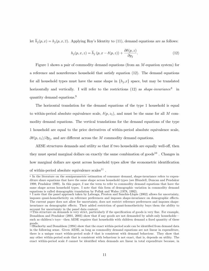
Figure 1 shows a pair of commodity demand equations (from an M-equation system) for

a reference and nonreference household that satisfy equation (12). The demand equations

for all household types must have the same shape in hj ,x space, but may be translated

horizontally and vertically. I will refer to the restrictions (12) as shape-invariance8 in

quantity demand equations.9

The horizontal translation for the demand equations of the type 1 household is equal

to within-period absolute equivalence scale, δ(p, z1), and must be the same for all M com-

modity demand equations. The vertical translations for the demand equations of the type

1 household are equal to the price derivatives of within-period absolute equivalence scale,

∂δ(p, z1)/∂pj, and are different across the M commodity demand equations.

AESE structures demands and utility so that if two households are equally well-off, then

they must spend marginal dollars on exactly the same combination of goods10 . Changes in

how marginal dollars are spent across household types allow the econometric identification

of within-period absolute equivalence scales11 .

8 In the literature on the semiparametric estimation of consumer demand, shape-invariance refers to expen-diture share equations that have the same shape across household types (see Blundell, Duncan and Pendakur1998; Pendakur 1999). In this paper, I use the term to refer to commodity demand equations that have thesame shape across household types. I note that this form of demographic variation in commodity demandequations is called demographic translation by Pollak and Wales (1978, 1992).9 I note that the panel approach taken by Labeaga, Preston and Sanchis-Llopis (2002) allows for uncertainty,imposes quasi-homotheticity on reference preferences and imposes shape-invariance on demographic effects.The current paper does not allow for uncertainty, does not restrict reference preferences and imposes shape-invariance on demographic effects. Their added restriction of quasi-homotheticity buys them the ability toaccount for uncertainty in the panel data context.10This structure on demands is very strict, particularly if the specification of goods is very fine. For example,Donaldson and Pendakur (2001, 2003) show that if any goods are not demanded by adult-only households–such as children’s toys–then AESE requires that households with children demand a fixed quantity of thesegoods.11Blackorby and Donaldson (1994) show that the exact within-period scale can be identified from demand datain the following sense. Given AESE, as long as commodity demand equations are not linear in expenditure,there is a unique exact within-period scale δ that is consistent with demand behaviour. They show thatany other within-period scale that is consistent with behaviour is not exact, that is, depends on utility. Theexact within-period scale δ cannot be identified when demands are linear in total expenditure because, in

11

Estimation of δ does not require specifying the shape of reference demand equations, as

would be required in a parametric approach. Under AESE, the shape of demand equations

is not critical to estimating lifetime scales. Rather, the distances between demand equations

across household types give the values of the exact within-period scales δ. Thus, estimation

of δ is amenable to semiparametric techniques, which are used in the next sections to estimate

exact within-period and lifetime scales.

4. The Data

Data from the 1990 and 1992 Canadian Family Expenditure Surveys (Statistics Canada,

1990, 1992) are used to estimate commodity demand equations for food, rent, clothing,

transportation operation12 , household operation and personal care at fixed prices13 . The

data come with weights that reflect the sampling frame, and the weights are incorporated

into the estimation of all the estimation14 .

Six household types are used: (i) childless single adults; (ii) childless adult couples; (iii)

adult couples with one child where the child is aged less than ten; (iv) adult couples with two

children where both children are aged less than ten; (v) adult couples with one child where

the child is aged ten to eighteen; and (vi) adult couples with two children where the eldest

child is aged ten to eighteen. Only households where all members are full-year members are

used.

this case, marginal dollars are always spent the same way, so that there are no changes to allow econometricidentification.12I use transportation expenditures net of vehicle purchases so that the transportation demand equationrepresents the flow of transportation services purchased.13In order to create a large enough sample for nonparametric estimation, I pool observations from the 1990and 1992 Family Expenditure Surveys and so treat all observations as if they are facing a single relative pricevector. Actual price changes over 1990-1992 for the five commodity groups used in this paper were (StatisticsCanada, 1993):

Food Rent Cloth. Trans. HH Op. Pers.4.4% 6.3% 10.4% 6.4% 5.3% 6.2%The transport price is a Fisher index of the prices of private transport operation and public transportation.

Clothing is the clear outlier to the pattern of stability in relative prices over this period. To pool observationsacross these two years, I deflate all demands and expenditures in 1992 by 6.2%, the Fisher index for the aboveprice changes.14Unweighted estimation and testing gives essentially identical results to those reported in the text.

12

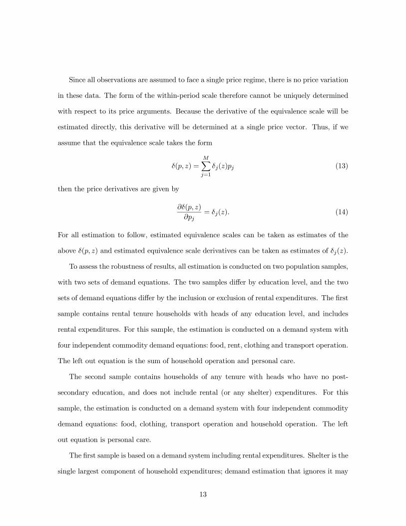
Since all observations are assumed to face a single price regime, there is no price variation

in these data. The form of the within-period scale therefore cannot be uniquely determined

with respect to its price arguments. Because the derivative of the equivalence scale will be

estimated directly, this derivative will be determined at a single price vector. Thus, if we

assume that the equivalence scale takes the form

δ(p, z) =MXj=1

δj(z)pj (13)

then the price derivatives are given by

∂δ(p, z)

∂pj= δj(z). (14)

For all estimation to follow, estimated equivalence scales can be taken as estimates of the

above δ(p, z) and estimated equivalence scale derivatives can be taken as estimates of δj(z).

To assess the robustness of results, all estimation is conducted on two population samples,

with two sets of demand equations. The two samples differ by education level, and the two

sets of demand equations differ by the inclusion or exclusion of rental expenditures. The first

sample contains rental tenure households with heads of any education level, and includes

rental expenditures. For this sample, the estimation is conducted on a demand system with

four independent commodity demand equations: food, rent, clothing and transport operation.

The left out equation is the sum of household operation and personal care.

The second sample contains households of any tenure with heads who have no post-

secondary education, and does not include rental (or any shelter) expenditures. For this

sample, the estimation is conducted on a demand system with four independent commodity

demand equations: food, clothing, transport operation and household operation. The left

out equation is personal care.

The first sample is based on a demand system including rental expenditures. Shelter is the

single largest component of household expenditures; demand estimation that ignores it may

13

be misleading. However, shelter expenditures are also less flexible than other expenditures,

which suggests that demand estimation which includes shelter may also be misleading.

The second sample differs by the exclusion of shelter expenditures, which may be exoge-

nous to current household budgeting15 . For example, if moving costs are high, households

will often choose the same accomodation year after year, even if total expenditure (or income

or utility) varies from year to year.

The second sample also differs in that it only includes households headed by people in the

lower part of the education distribution, a population that has lower expected lifetime wealth,

and lower variance in lifetime wealth, than the entire sample. The a priori plausibility of

AESE’s fixed absolute equivalence scales is strengthened for this sample because here we

require that absolute equivalence scales be fixed across a sample of households with low

mean and variance of lifetime wealth, rather than across the entire population of households.

Table 1 offers data means for the six household types used in this paper. The demand

equations modelled in this paper make up the bulk of household current consumption. The

demands modeled in sample 1 make up between 65% and 70% of current consumption, and

those modeled in sample 2 make up 45% to 51% of current consumption.

15If shelter expenditures are weakly separable from the goods in the estimated demand system, then we mayexclude them. However, if they are not, then estimation should condition on shelter expenditures. This isdifficult to do in the semiparametric context.

14

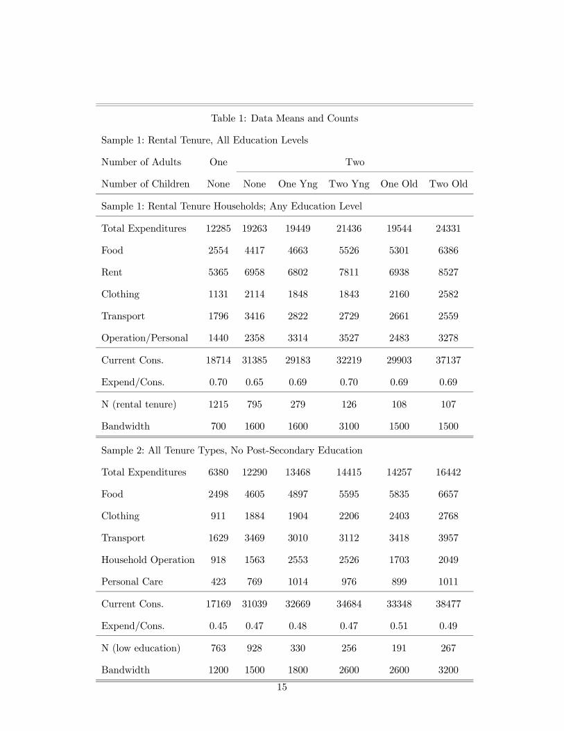
Table 1: Data Means and Counts

Sample 1: Rental Tenure, All Education Levels

Number of Adults One Two

Number of Children None None One Yng Two Yng One Old Two Old

Sample 1: Rental Tenure Households; Any Education Level

Total Expenditures 12285 19263 19449 21436 19544 24331

Food 2554 4417 4663 5526 5301 6386

Rent 5365 6958 6802 7811 6938 8527

Clothing 1131 2114 1848 1843 2160 2582

Transport 1796 3416 2822 2729 2661 2559

Operation/Personal 1440 2358 3314 3527 2483 3278

Current Cons. 18714 31385 29183 32219 29903 37137

Expend/Cons. 0.70 0.65 0.69 0.70 0.69 0.69

N (rental tenure) 1215 795 279 126 108 107

Bandwidth 700 1600 1600 3100 1500 1500

Sample 2: All Tenure Types, No Post-Secondary Education

Total Expenditures 6380 12290 13468 14415 14257 16442

Food 2498 4605 4897 5595 5835 6657

Clothing 911 1884 1904 2206 2403 2768

Transport 1629 3469 3010 3112 3418 3957

Household Operation 918 1563 2553 2526 1703 2049

Personal Care 423 769 1014 976 899 1011

Current Cons. 17169 31039 32669 34684 33348 38477

Expend/Cons. 0.45 0.47 0.48 0.47 0.51 0.49

N (low education) 763 928 330 256 191 267

Bandwidth 1200 1500 1800 2600 2600 3200

15

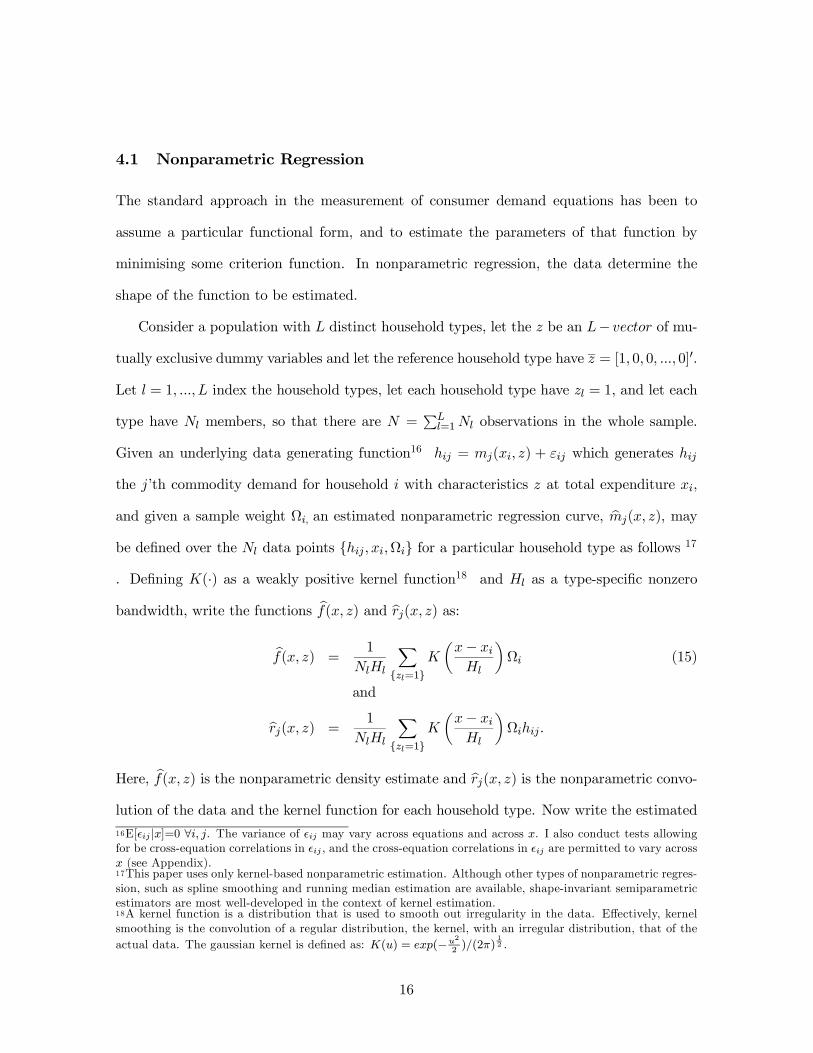
4.1 Nonparametric Regression

The standard approach in the measurement of consumer demand equations has been to

assume a particular functional form, and to estimate the parameters of that function by

minimising some criterion function. In nonparametric regression, the data determine the

shape of the function to be estimated.

Consider a population with L distinct household types, let the z be an L− vector of mu-tually exclusive dummy variables and let the reference household type have z = [1, 0, 0, ..., 0]0.

Let l = 1, ..., L index the household types, let each household type have zl = 1, and let each

type have Nl members, so that there are N =PLl=1Nl observations in the whole sample.

Given an underlying data generating function16 hij = mj(xi, z) + εij which generates hij

the j’th commodity demand for household i with characteristics z at total expenditure xi,

and given a sample weight Ωi, an estimated nonparametric regression curve, bmj(x, z), maybe defined over the Nl data points hij, xi,Ωi for a particular household type as follows 17

. Defining K(·) as a weakly positive kernel function18 and Hl as a type-specific nonzero

bandwidth, write the functions bf(x, z) and brj(x, z) as:bf(x, z) =

1

NlHl

Xzl=1

K

µx− xiHl

¶Ωi (15)

and

brj(x, z) =1

NlHl

Xzl=1

K

µx− xiHl

¶Ωihij.

Here, bf(x, z) is the nonparametric density estimate and brj(x, z) is the nonparametric convo-lution of the data and the kernel function for each household type. Now write the estimated

16E[²ij |x]=0 ∀i, j. The variance of ²ij may vary across equations and across x. I also conduct tests allowingfor be cross-equation correlations in ²ij , and the cross-equation correlations in ²ij are permitted to vary acrossx (see Appendix).17This paper uses only kernel-based nonparametric estimation. Although other types of nonparametric regres-sion, such as spline smoothing and running median estimation are available, shape-invariant semiparametricestimators are most well-developed in the context of kernel estimation.18A kernel function is a distribution that is used to smooth out irregularity in the data. Effectively, kernelsmoothing is the convolution of a regular distribution, the kernel, with an irregular distribution, that of theactual data. The gaussian kernel is defined as: K(u) = exp(−u2

2 )/(2π)12 .

16

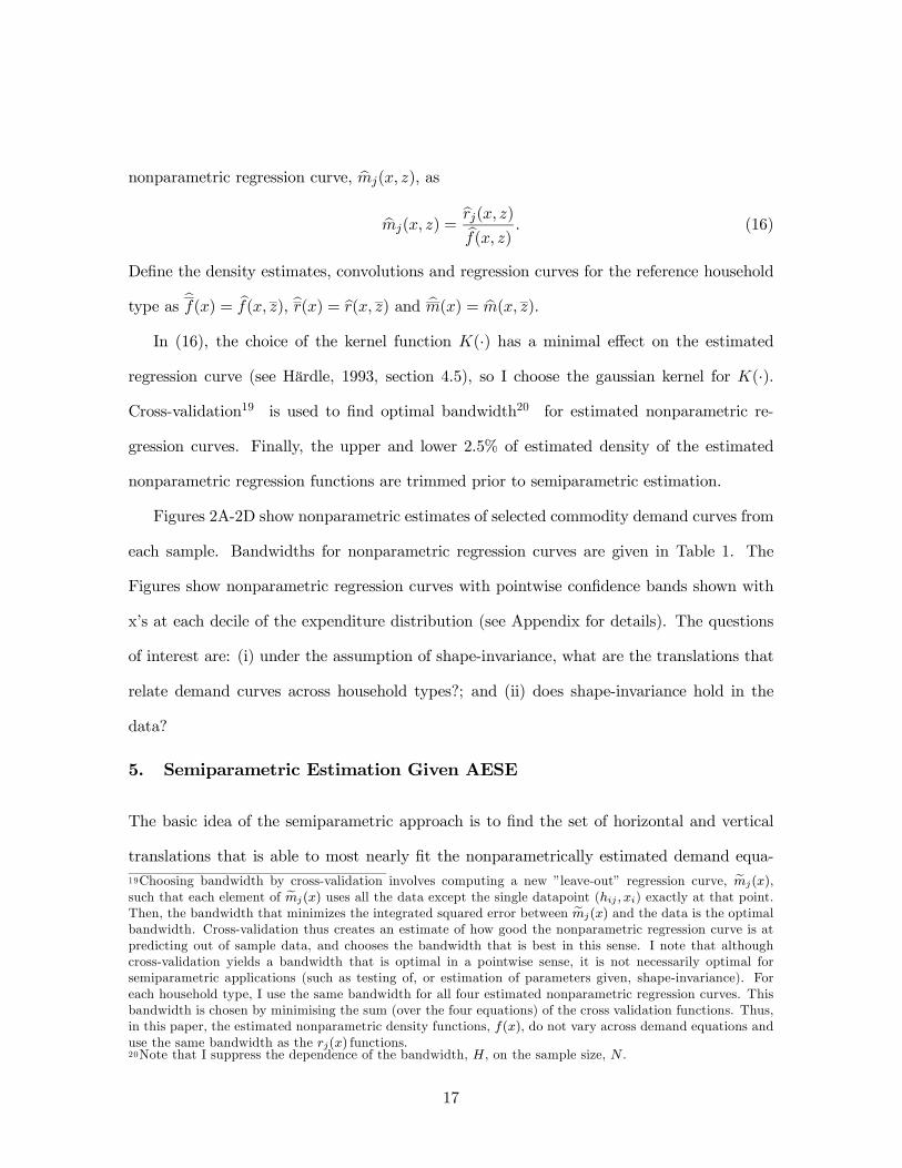
nonparametric regression curve, bmj(x, z), asbmj(x, z) = brj(x, z)bf(x, z) . (16)

Define the density estimates, convolutions and regression curves for the reference household

type as bf(x) = bf(x, z), br(x) = br(x, z) and bm(x) = bm(x, z).In (16), the choice of the kernel function K(·) has a minimal effect on the estimated

regression curve (see Härdle, 1993, section 4.5), so I choose the gaussian kernel for K(·).Cross-validation19 is used to find optimal bandwidth20 for estimated nonparametric re-

gression curves. Finally, the upper and lower 2.5% of estimated density of the estimated

nonparametric regression functions are trimmed prior to semiparametric estimation.

Figures 2A-2D show nonparametric estimates of selected commodity demand curves from

each sample. Bandwidths for nonparametric regression curves are given in Table 1. The

Figures show nonparametric regression curves with pointwise confidence bands shown with

x’s at each decile of the expenditure distribution (see Appendix for details). The questions

of interest are: (i) under the assumption of shape-invariance, what are the translations that

relate demand curves across household types?; and (ii) does shape-invariance hold in the

data?

5. Semiparametric Estimation Given AESE

The basic idea of the semiparametric approach is to find the set of horizontal and vertical

translations that is able to most nearly fit the nonparametrically estimated demand equa-19Choosing bandwidth by cross-validation involves computing a new ”leave-out” regression curve, emj(x),such that each element of emj(x) uses all the data except the single datapoint (hij , xi) exactly at that point.Then, the bandwidth that minimizes the integrated squared error between emj(x) and the data is the optimalbandwidth. Cross-validation thus creates an estimate of how good the nonparametric regression curve is atpredicting out of sample data, and chooses the bandwidth that is best in this sense. I note that althoughcross-validation yields a bandwidth that is optimal in a pointwise sense, it is not necessarily optimal forsemiparametric applications (such as testing of, or estimation of parameters given, shape-invariance). Foreach household type, I use the same bandwidth for all four estimated nonparametric regression curves. Thisbandwidth is chosen by minimising the sum (over the four equations) of the cross validation functions. Thus,in this paper, the estimated nonparametric density functions, f(x), do not vary across demand equations anduse the same bandwidth as the rj(x) functions.20Note that I suppress the dependence of the bandwidth, H, on the sample size, N .

17

tions of two household types. The search algorithm is a simple gridsearch across a span

of translations which seeks the minimum value of a loss function proposed by Pinkse and

Robinson (1995). This loss function measures the distance between demand functions after

translation.

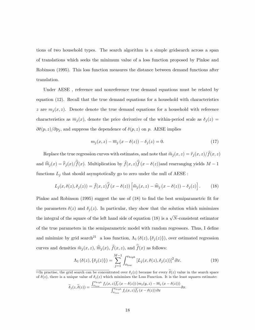
Under AESE , reference and nonreference true demand equations must be related by

equation (12). Recall that the true demand equations for a household with characteristics

z are mj(x, z). Denote denote the true demand equations for a household with reference

characteristics as mj(x), denote the price derivative of the within-period scale as δj(z) =

∂δ(p, z)/∂pj , and suppress the dependence of δ(p, z) on p. AESE implies

mj(x, z)−mj (x− δ(z))− δj(z) = 0. (17)

Replace the true regression curves with estimates, and note that bmj(x, z) = brj(x, z)/ bf(x, z)and bmj(x) = brj(x)/bf(x). Multiplication by bf(x, z)bf (x− δ(z))and rearranging yields M − 1functions Lj that should asymptotically go to zero under the null of AESE :

Lj(x, δ(z), δj(z)) = bf(x, z)bf (x− δ(z))h bmj(x, z)− bmj (x− δ(z))− δj(z)

i. (18)

Pinkse and Robinson (1995) suggest the use of (18) to find the best semiparametric fit for

the parameters δ(z) and δj(z). In particular, they show that the solution which minimizes

the integral of the square of the left hand side of equation (18) is a√N-consistent estimator

of the true parameters in the semiparametric model with random regressors. Thus, I define

and minimize by grid search21 a loss function, Λ1 (δ(z), δj(z)), over estimated regressioncurves and densities bmj(x, z), bmj(x), bf(x, z), and bf(x) as follows:

Λ1 (δ(z), δj(z)) =M−1Xj=1

Z xhigh

xlow

[Lj(x, δ(z), δj(z))]2 ∂x. (19)

21In practise, the grid search can be concentrated over δj(z) because for every eδ(z) value in the search spaceof δ(z), there is a unique value of δj(z) which minimises the Loss Function. It is the least squares estimate:

eδj(z,eδ(z)) = R xhighxlowfj(x, z)fj (x− δ(z)) (mj(y, z)−mj (x− δ(z)))R xhigh

xlowfj(x, z)fj (x− δ(z))∂x

∂x.

18

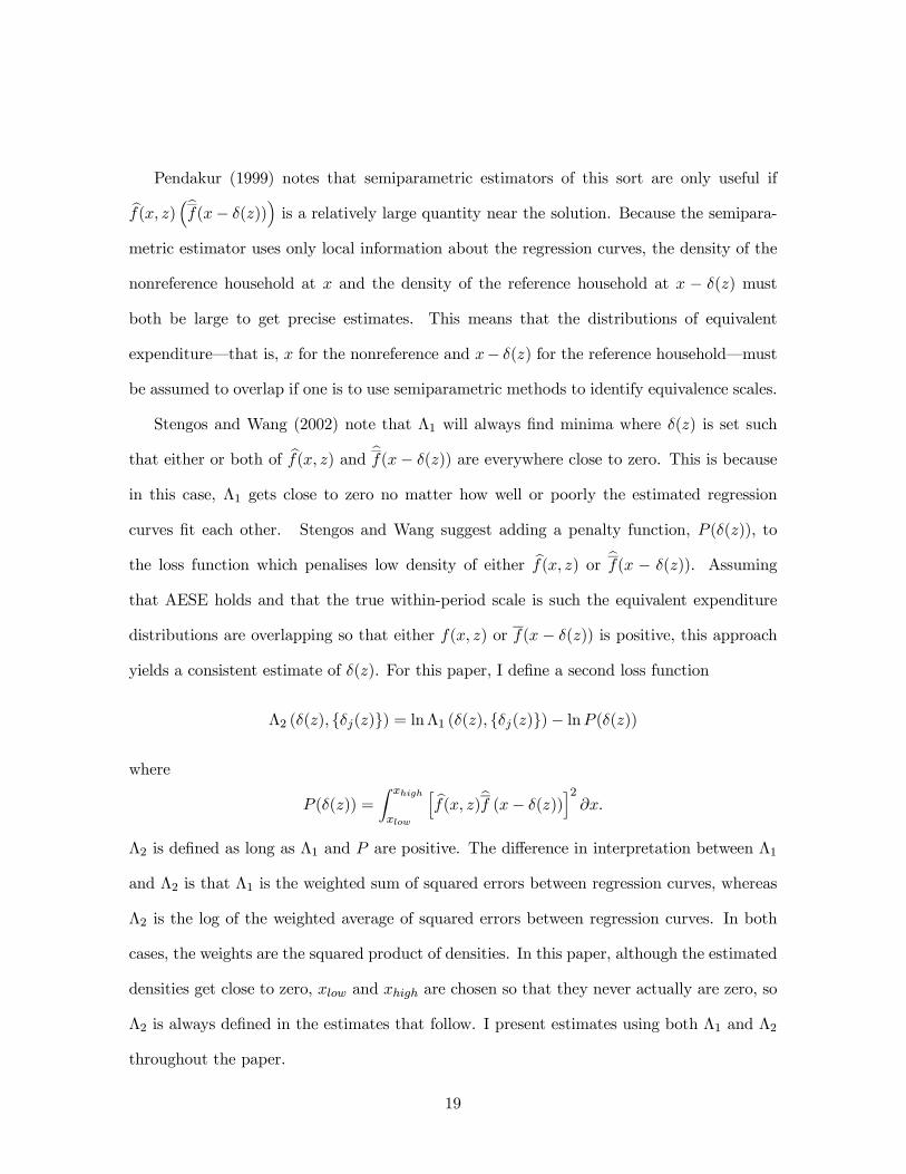
Pendakur (1999) notes that semiparametric estimators of this sort are only useful if

bf(x, z)³bf(x− δ(z))´is a relatively large quantity near the solution. Because the semipara-

metric estimator uses only local information about the regression curves, the density of the

nonreference household at x and the density of the reference household at x − δ(z) must

both be large to get precise estimates. This means that the distributions of equivalent

expenditure–that is, x for the nonreference and x− δ(z) for the reference household–must

be assumed to overlap if one is to use semiparametric methods to identify equivalence scales.

Stengos and Wang (2002) note that Λ1 will always find minima where δ(z) is set such

that either or both of bf(x, z) and bf(x− δ(z)) are everywhere close to zero. This is because

in this case, Λ1 gets close to zero no matter how well or poorly the estimated regression

curves fit each other. Stengos and Wang suggest adding a penalty function, P (δ(z)), to

the loss function which penalises low density of either bf(x, z) or bf(x − δ(z)). Assuming

that AESE holds and that the true within-period scale is such the equivalent expenditure

distributions are overlapping so that either f(x, z) or f(x− δ(z)) is positive, this approach

yields a consistent estimate of δ(z). For this paper, I define a second loss function

Λ2 (δ(z), δj(z)) = lnΛ1 (δ(z), δj(z))− lnP (δ(z))

where

P (δ(z)) =Z xhigh

xlow

h bf(x, z)bf (x− δ(z))i2∂x.

Λ2 is defined as long as Λ1 and P are positive. The difference in interpretation between Λ1

and Λ2 is that Λ1 is the weighted sum of squared errors between regression curves, whereas

Λ2 is the log of the weighted average of squared errors between regression curves. In both

cases, the weights are the squared product of densities. In this paper, although the estimated

densities get close to zero, xlow and xhigh are chosen so that they never actually are zero, so

Λ2 is always defined in the estimates that follow. I present estimates using both Λ1 and Λ2

throughout the paper.

19

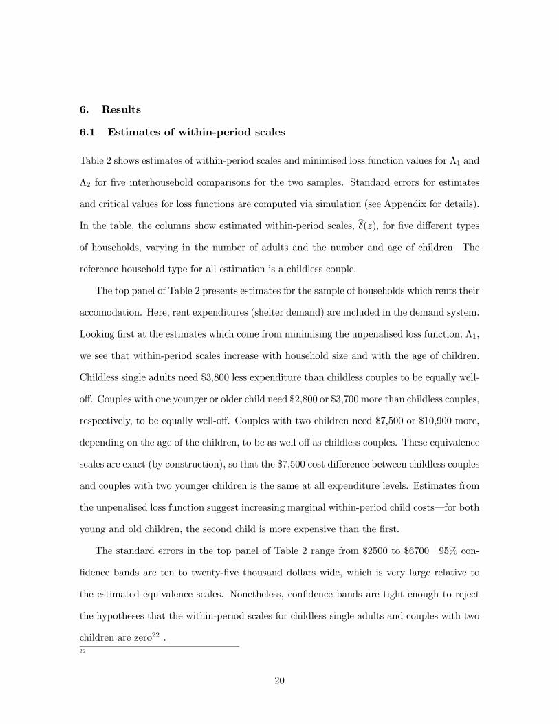
6. Results

6.1 Estimates of within-period scales

Table 2 shows estimates of within-period scales and minimised loss function values for Λ1 and

Λ2 for five interhousehold comparisons for the two samples. Standard errors for estimates

and critical values for loss functions are computed via simulation (see Appendix for details).

In the table, the columns show estimated within-period scales, bδ(z), for five different typesof households, varying in the number of adults and the number and age of children. The

reference household type for all estimation is a childless couple.

The top panel of Table 2 presents estimates for the sample of households which rents their

accomodation. Here, rent expenditures (shelter demand) are included in the demand system.

Looking first at the estimates which come from minimising the unpenalised loss function, Λ1,

we see that within-period scales increase with household size and with the age of children.

Childless single adults need $3,800 less expenditure than childless couples to be equally well-

off. Couples with one younger or older child need $2,800 or $3,700 more than childless couples,

respectively, to be equally well-off. Couples with two children need $7,500 or $10,900 more,

depending on the age of the children, to be as well off as childless couples. These equivalence

scales are exact (by construction), so that the $7,500 cost difference between childless couples

and couples with two younger children is the same at all expenditure levels. Estimates from

the unpenalised loss function suggest increasing marginal within-period child costs–for both

young and old children, the second child is more expensive than the first.

The standard errors in the top panel of Table 2 range from $2500 to $6700–95% con-

fidence bands are ten to twenty-five thousand dollars wide, which is very large relative to

the estimated equivalence scales. Nonetheless, confidence bands are tight enough to reject

the hypotheses that the within-period scales for childless single adults and couples with two

children are zero22 .22

20

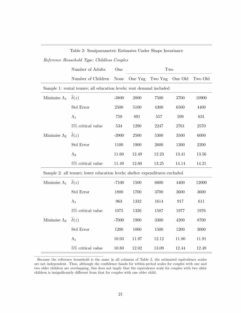
Table 2: Semiparametric Estimates Under Shape Invariance

Reference Household Type: Childless Couples

Number of Adults One Two

Number of Children None One Yng Two Yng One Old Two Old

Sample 1: rental tenure; all education levels; rent demand included

Minimise Λ1 bδ(z) -3800 2800 7500 3700 10900

Std Error 2500 5100 4300 6500 4400

Λ1 759 891 557 599 631

5% critical value 534 1290 2247 2761 2570

Minimise Λ2 bδ(z) -3900 2500 5300 3500 6000

Std Error 1100 1900 2600 1300 2200

Λ2 11.60 12.49 12.23 13.41 13.56

5% critical value 11.49 12.60 13.25 14.14 14.21

Sample 2: all tenure; lower education levels; shelter expenditures excluded

Minimise Λ1 bδ(z) -7100 1500 6600 4400 12000

Std Error 1800 1700 3700 3600 3600

Λ1 963 1332 1614 917 611

5% critical value 1075 1326 1587 1977 1976

Minimise Λ2 bδ(z) -7000 1900 3300 4200 8700

Std Error 1200 1000 1500 1200 3000

Λ1 10.93 11.97 12.12 11.80 11.91

5% critical value 10.80 12.02 13.09 12.44 12.49

Because the reference household is the same in all columns of Table 2, the estimated equivalence scalesare not independent. Thus, although the confidence bands for within-period scales for couples with one andtwo older children are overlapping, this does not imply that the equivalence scale for couples with two olderchildren is insignificantly different from that for couples with one older child.

21

Looking next at the results for sample 1 which minimise the penalised loss function, Λ2,

we see qualitatively similar results in that within-period scales increase with household size

and with the age of children. Here, the estimated within-period scales for childless single

adults and for couples with one child are similar to those estimated with the unpenalised

loss function. However, the estimates for couples with two children are somewhat smaller.

The estimated within-period scales for a couple with two young children and with two older

children are $5300 and $6000, respectively, which suggests approximately the same marginal

within-period cost for the first and second child.

The estimates using the penalised loss function are also much more precisely estimated,

which is due to the fact that they favour estimates which are informed by a lot of data. The

simulated standard errors are about half as large as those simulated with the unpenalised

estimator.

The bottom panel of Table 2 presents estimates for the sample of households of any

accomodation tenure where the household head has no post-secondary education. Here,

shelter expenditures (including rent) are excluded from the demand system.

Looking first at the results using the unpenalised loss function, Λ1, we see that childless

single adults need $7,100 less expenditure than childless couples to be equally well-off. Es-

timated within-period scales again suggest that young children cost less than older children

and that the second child costs more than the first child.

Turning now to the results using the penalised loss function, Λ2, we see a similar estimate

of the within-period scale for childless single adults and for couples with one child, but much

smaller estimated within-period scales for couples with two children. For couples with young

children, the estimated within-period scales are $1900 and $3300 for one and two children,

respectively. For couples with older children, the estimated within-period scales are $4200

and $8700 for one and two children, respectively. These estimates suggest approximately

constant marginal within-period child costs.

22

Three differences between the results for the two samples should be noted. First, because

estimates for sample 2 exclude shelter from total expenditure in the demand system and

use a lower expenditure population sample, the equivalence scales here are larger relative to

average household expenditure than those in the top panel. Average household expenditure

for childless couples is more than 50% larger in sample 1 than in sample 2 (see Table 1).

Second, the estimates in the bottom panel have smaller standard errors, allowing for tighter

confidence bands. Third, because sample 2 is characterised by lower variance of education,

expenditure and lifetime wealth than sample 1, the exactness assumption is more intuitively

plausible.

If we take the penalised estimates as more trustworthy, two broad conclusions may be

reached. First, these results suggest that the marginal cost of children is approximately

constant. Second, these results suggest that families the with older children have much

greater within-period scales than families with younger children. However, because young

children become older children, this distinction may be misleading. In the next section, I

calculate lifetime scales by adding up within-period absolute equivalence scales.

6.2 Estimates of lifetime scales

Given AESE, perfect foresight and perfect credit markets, knowledge of the exact within-

period scales shown in Table 2 allows the calculation of lifetime scales as∆(P,Z) =PTt=1 ρ

tδ(pt, zt)

where ρt is the credit market discount from period 1 to period t. These lifetime scales are

measured in real expenditure. Table 4 shows lifetime scales for selected demographic profiles

based on the estimates in Table 2 and a real interest rate of 3% per year. Relative prices are

assumed constant throughout the fifty year adult lifetime.

For comparison, Table 3 shows estimated lifetime scales from Pashardes (1991) and from

Banks, Blundell and Preston (1994). Their lifetime scales are not exact, that is, they depend

on the level of lifetime utility at which interhousehold comparisons are made. Lifetime

23

scales from Pashardes (1991) and Banks, Blundell and Preston (1994) are evaluated at mean

expenditure for childless couples23 .

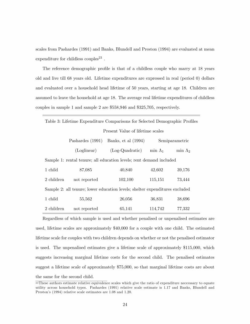
The reference demographic profile is that of a childless couple who marry at 18 years

old and live till 68 years old. Lifetime expenditures are expressed in real (period 0) dollars

and evaluated over a household head lifetime of 50 years, starting at age 18. Children are

assumed to leave the household at age 18. The average real lifetime expenditures of childless

couples in sample 1 and sample 2 are $558,946 and $325,705, respectively.

Table 3: Lifetime Expenditure Comparisons for Selected Demographic Profiles

Present Value of lifetime scales

Pashardes (1991) Banks, et al (1994) Semiparametric

(Loglinear) (Log-Quadratic) min Λ1 min Λ2

Sample 1: rental tenure; all education levels; rent demand included

1 child 87,085 40,840 42,602 39,176

2 children not reported 102,100 115,151 73,444

Sample 2: all tenure; lower education levels; shelter expenditures excluded

1 child 55,562 26,056 36,831 38,696

2 children not reported 65,141 114,742 77,332

Regardless of which sample is used and whether penalised or unpenalised estimates are

used, lifetime scales are approximately $40,000 for a couple with one child. The estimated

lifetime scale for couples with two children depends on whether or not the penalised estimator

is used. The unpenalised estimates give a lifetime scale of approximately $115,000, which

suggests increasing marginal lifetime costs for the second child. The penalised estimates

suggest a lifetime scale of approximately $75,000, so that marginal lifetime costs are about

the same for the second child.23These authors estimate relative equivalence scales which give the ratio of expenditure neccessary to equateutility across household types. Pashardes (1991) relative scale estimate is 1.17 and Banks, Blundell andPreston’s (1994) relative scale estimates are 1.08 and 1.20.

24

Although the estimates of lifetime scales do not vary much across the samples, their rela-

tive importance does differ. Consider the size of the lifetime scales using penalised estimates

relative to the lifetime real expenditure of the average childless couple. For sample 1, the

lifetime scale for a couple with one child represents approximately 7% of real lifetime expen-

diture; for sample 2, the lifetime scale for a couple with one child represents almost 12% of

real lifetime expenditure (shelter expenditures are not included for sample 2).

Looking at the estimates for sample 1, the semiparametric estimates of lifetime scales

for couples with one child are quite similar to those of Banks, Blundell and Preston (1994),

but suggest much lower lifetime scales than Pashardes (1991). However, whereas Banks,

Blundell and Preston (1994) find increasing marginal costs for the second child, the penalised

semiparametric estimates find approximately constant marginal lifetime child costs.

Turning to the estimates for sample 2, the comparison with Banks, Blundell and Preston

has the opposite pattern. The penalised semiparametric estimates are much the same as

for sample 1, but the scale from Banks, Blundell and Preston suggests much lower lifetime

costs. This is due to the fact that they report ratio scales which scale expenditure rather

than translate expenditure. It should be noted that the estimates of Banks, Blundell and

Preston (1994) and Pashardes (1991) are based on samples that more closely resemble my

sample 1. Thus, I am inclined to take the closeness of my sample 1 estimates to those of

Banks, Blundell and Preston as corroborative.

If we take the penalised estimates as more trustworthy, and take the sample 2 estimates

as more useful given the strictness of AESE, these results suggest that the lifetime cost of

one child is approximately $39,000 and the lifetime cost of two children is about $77,000.

The semiparametric estimates of within-period scales shown in Table 2 and the calcu-

lations of lifetime scales shown in Table 3 are contingent on AESE holding in the data. If

the AESE restrictions (12) do not hold in the demand data, then AESE cannot hold in the

within-period expenditure function, and the estimates of within-period and lifetime scales

25

are rendered meaningless. The next section tests the null hypothesis given by the AESE

restrictions (12) against a fully nonparametric alternative.

6.3 Tests of Exactness

Table 2 shows the minimised value of the loss functions, Λ1 and Λ2. The shape-invariance

restrictions are tested by asking whether or not the minimised values of these loss functions

are large compared with loss functions simulated in an environment where shape-invariance

holds by construction (see Appendix 1 for details). Below each of the minimised loss function

values, Table 2 shows the 5% critical value of the loss function from simulated distributions

where shape-invariance holds by construction. The 5% critical value is equal to the 95’th

percentile of the simulated distribution.

Looking first at the results for sample 1, for the comparison of childless single adults to

childless couples, the minimised values of Λ1 and Λ2 are both high relative to the distribu-

tions of loss function values where shape-invariance holds by construction. So, we reject the

hypothesis that shape-invariance, and therefore AESE, holds for this interhousehold com-

parison.

For the other comparisons, the observed minimised values of Λ1 and Λ2 are smaller than

the 5% critical values. Thus, for these inter-household comparisons shape-invariance, and

therefore AESE, is not rejected by the data.

Of course, failing to reject the hypothesis of shape-invariance could be due to either the

truth of AESE or to imprecision in estimation resulting from a paucity of data. The fact that

the only rejection is for the comparison of childless single adults and childless couples–the

two largest household types–should caution us to consider the latter possibility.

It should be noted that non-rejection of AESE does not imply acceptance of AESE for

reasons pointed out by Pollak and Wales (1979) and Blundell and Lewbel (1991). Only the

ordinal features of the utility function can be tested–the equality of indirect utility across

26

household types in equation (11) is untestable. Thus, it is helpful to have estimates for which

the a priori plausibility of AESE is stronger. For this we turn to the results for sample 2.

For sample 2, most of the minimised loss function values are lower than the 5% critical

value. Two exceptions are the penalised semiparametric estimate for single childless adults

and the unpenalised semiparametric estimate for couples with one young child. If we take

the penalised estimates as more trustworthy, then for this sample of less educated and lower

expenditure households, we do not reject the shape invariance restrictions implied by AESE

for comparisons of childless couples and couples with children. Thus, the lifetime scales

reported in Table 3 may be meaningful.

7. Conclusions

If within-period expenditure functions satisfy Absolute Equivalence Scale Exactness (AESE),

then within-period equivalence scales, defined as the difference in expenditure needs across

household types, are independent of utility. Under perfect information and credit markets,

if within-period expenditure functions satisfy AESE, then lifetime equivalence scales equal

the present value of exact within-period scales and are independent of lifetime utility.

Given AESE, commodity demand equations must have the same shape across household

types, and within-period scales are identifiable from demand data via semiparametric esti-

mation. Within-period scales are estimated using semiparametric methods and Canadian

expenditure data. These scales increase with the age and number of children. The hypothe-

ses that commodity demand equations have the same shape across household types are not

rejected for most interhousehold comparisons. Therefore the restrictions implied by Absolute

Equivalence Scale Exactness are not rejected.

Using semiparametric estimates of exact within-period scales, lifetime scales are approx-

imately $39,000 for one child and $77,000 for two children. These lifetime scales amount to

approximately 12% of lifetime real expenditure for each child for the average childless couple.

27

REFERENCES

Banks, James, Richard Blundell and Ian Preston (1994), “Estimating the In-tertemporal Costs of Children” in R. Blundell, I. Preston, and I. Walker (eds),The Economics of Household Behaviour, Cambridge University Press, Cambridge, pp.51-69.

Banks, James, Richard Blundell and Arthur Lewbel (1994b), “Quadratic Engel Curves,Indirect Tax Reform and Welfare Measurement”, University College of London Discus-sion Paper 94-04.

Banks, Blundell and Lewbel (1997), “Quadratic Engel Curves and Consumer Demand”,Review of Economics and Statistics, 79(4), pp 527-539.

Blackorby, Charles an David Donaldson (1989), “Adult Equivalence Scales, Interper-sonal Comparisons of Well-Being and Applied Welfare Economics”, University of BritishColumbia, Department of Economics Discussion Paper 89-24.

— (1991), “Adult-Equivalence Scales, Interpersonal Comparisons of Well-Being and Applied Welfare Economics,” in J. Elster and J. Roemer (eds),Interpersonal Comparisons of Well-Being, Cambridge University Press, Cambridge, pp164-199.

— (1993), “Adult Equivalence Scales and the Economic Implementation of InterpersonalComparisons of Well-Being”, Social Choice and Welfare, 10, pp 335-361.

— (1994), “Measuring the Costs of Children: A Theoretical Framework,” in R. Blundell,I. Preston, and I. Walker (eds), The Economics of Household Behaviour, CambridgeUniversity Press, Cambridge, pp. 51-69.

Blundell, Richard, Martin Browning and Costas Meghir (1994), “Con-sumer Demand and the Life-Cycle Allocation of Household Expenditures“,Review of Economic Studies, 61(1), January 1994, pp 57-80.

Blundell, Richard, Alan Duncan and Krishna Pendakur (1998), “Semiparametric Esti-mation of Consumer Demand”, Journal of Applied Econometrics, 13, pp 435-461.

Blundell, Richard and Arthur Lewbel (1991), “Information Content of EquivalenceScales”, Journal of Econometrics, 50, pp 49-68.

Blundell, Richard, Panos Pashardes and Weber Guglielmo (1993), “What Do We LearnAbout Consumer Demand Patterns from Micro Data?”, American Economic Review,83(3), June, pages 570-97.

Browning, Martin (1989), “The Effects of Children on Demand Behaviour and House-hold Welfare”, Unpublished mimeo, McMaster University.

— (1992), “Children and Household Behaviour”, Journal of Economic Literature, 30,Sep, pp 1434-75.

Dickens, Richard, Vanessa. Fry and Panos Pashardes (1993), “Nonlinearities, Aggrega-tion and Equivalence Scales”, Economic Journal, 103, March 1993, pp 359-368.

Donaldson, David and Krishna Pendakur (2001), ”Expenditure-Dependent EquivalenceScales”, unpublished working paper, Department of Economics, Simon Fraser Univer-sity, available at www.sfu.ca~/pendakur.

28

Donaldson, David and Krishna Pendakur (2003), ”Equivalent-Expenditure Functionsand Expenditure-Dependent Equivalence Scales”, Journal of Public Economics, forth-coming.

Gozalo, Pedro (1997), “Nonparametric Bootstrap analysis with applications to demo-graphic effects in demand functions”, Journal of Econometrics, 81, pp 357-393.

Härdle, Wolfgang and G. Kelly (1987), “Nonparametric Kernel Regression Estimation—Optimal Choice of Bandwidth”, Statistics, 18, pp 21-35.

Härdle, Wolfgang (1993), Applied Nonparametric Regression, Cambridge UniversityPress, New York.

Härdle, Wolfgang and J.S. Marron (1990), “Semiparametric Comparison of RegressionCurves”, Annals of Statistics, 18(1), pp 63-89.

Keen, Michael (1990), “Welfare Analysis and Intertemporal Substitution”,Journal of Public Economics, 42(1), pages 47-66.

Kneip, Alois (1994), “Nonparametric Estimation of Common Regressors for SimilarCurve Data”, Annals of Statistics, 22(3), pp 1386-1427.

Kneip, Alois and Joachim Engel (1995), “Model Estimation in Nonlinear RegressionUnder Shape Invariance”, Annals of Statistics, 23(2), pp 551-570.

Jorgenson, Dale, Lawrence Lau and Tom Stoker (1960), “The Trancendental Log-arithmic Model of Aggregate Consumer Behaviour”, reprinted in Robert Bassmanand George Rhodes (eds)., Advances in Econometrics: A Research Manual, JAI Press,Greenwich, CT, 1982.

Labeaga, Jose, Ian Preston and Juan A. Sanchis-Llopis (2002), ”Demand, Childbirthand the Cost of Babies: Evidence from Spanish Panel Data” unpublished working paper,Department of Economics, University College London.

Lewbel, Arthur (1989), “Identification and Estimation of Equivalence Scales UnderWeak Separability”, Review of Economic Studies. 52(6), pp 311-316.

— (1989b), “Household Equivalence Scales and Welfare Comparisons”,Journal of Public Economics, 39(3), August pages 377-91.

— (1991), “Cost of Characteristics Indices and Household Equivalence Scales”,European Economic Review, 35(6), August 1991, pages 1277-93.

Nelson, Julie (1991), “Independent of a Base Equivalence Scale Estimation”. unpub-lished mimeo, University of California, Davis.

Pashardes, Panos (1991), “Contemporaneous and Intertemporal Child Costs”Economic Journal.

Pashardes, Panos (1995), “Equivalence Scales in a Rank-3 Demand System”,Journal of Public Economics, 58, pp 143-158.

Pendakur, Krishna (1999), “Semiparametric Estimates and Tests of Base-IndependentEquivalence Scales”, Journal of Econometrics, 88(1), pages 1-40.

Phipps, Shelley (1996), “Canadian Child Benefits: Behavioural Consequences and In-come Adequacy”, Canadian Public Policy 21(1).

29

— (1990), “Price Sensitive Equivalence Scale for Canada”, unpublished, Dalhousie Uni-versity.

Pinkse, C.A.P. and P.M. Robinson (1995), “Pooling Nonparametric Estimates of Re-gression Functions with a Similar Shape”, in G. Maddala, P. Phillips and T.N. Srinivisan(eds), Advances in Econometrics and Quantitative Economics, pp. 172-195.

Pollak, Robert and Terence J. Wales (1978), “Estimation of Complete Demand Sys-tems from Household Budget Data: The Linear and Quadratic Expenditure Systems”,American Economic Review, 68(3), June 1978, pp 348-359.

- (1979), “Welfare Comparisons and Equivalence Scales” American Economic Review,69(2), May 1979, pp 216-21.

- (1992), Demand System Specification and Estimation, Oxford University Press, Lon-don, UK.

Pollak, Robert (1991), “Welfare Comparisons and Situation Comparisons”,Journal of Econometrics, 50, pp 31-48.

Stengos, Thanassis and Dianqin Wang (2002), “Estimates of Semiparametric IncomeEquivalence Scales” unpublished working paper, Department of Economics, Universityof Guelph.

U.S. House of Representatives, Committee on Ways and Means (1994), “Where YourMoney Goes...The 1994-1995 Green Book”, Washington D.C, U.S. Government Printers.

Working, H. (1943), “Statistical Laws of Family Expenditure”,Journal of the American Statistical Association, 38, pp 43-56.

8. Appendix: Simulation Methodology

8.1 Confidence Bands for Nonparametric Regression Curves

Pointwise confidence bands for nonparametric regression curves in Figures 2A-2C are esti-

mated via Smooth Conditional Moment Bootstrap. See Gozalo (1997) for details.

8.2 Distributions for Semiparametric Estimates

I estimate small-sample distributions for estimated equivalence scales, equivalence scale deriv-

atives and loss functions via monte carlo simulations, following Pendakur (1999). Under

shape-invariance, the underlying true regression curves are related by horizontal and vertical

shifts, δ(z) and δk(z). I construct bootrap samples maintaining this restriction, and sim-

ulate the distribution of the semiparametric estimates of δ(z), δk(z) and L(δ(z);δk(z)).

Although Pinkse and Robinson (1995) show that these random variables are asymptotically

30

normal, the small sample simulations suggest that while δ(z) and δk(z) have roughly sym-

metric distributions, the distribution of L(δ(z);δk(z)) is right-hand skewed. Thus, standard

errors for L(δ(z);δk(z)) should be interpreted with caution: standard errors may be difficult

to interpret when the distribution is non-normal.

To estimate the small-sample distributions of semiparametric estimates computed on N1

reference and N2 nonreference data points, I use the percentile-t method as follows.

Step 1: Estimate the reference and nonreference nonparametric regression curves, bmj(x)and bmj(x), over each data point, xi, for theM−1 independent commodity demand equations.Create empirical errors as ²ij = hij − bmij . For each observation of xi, there is therefore aquadruple of the M − 1 empirical errors.

To generate the simulated error distribution, use Gozalo’s (1997) Smooth Conditional

Moment (SCM) Bootstrap as follows. Estimate the conditional second and third moments

of the error distributions as nonparametric regressions of ²2ij and ²3ij . Use these moments to

generate a mean zero simulated error distribution with second and third moments matching

those in the empirical error distribution via the Golden Section (see Gozalo 1997).

For each of the N1 and N2 xi, computeM−1 restricted nonparametric regression curves,mNULLj (xi), that satisfy the null hypothesis of shape-invariance. These are computed by

translating the nonreference data by the estimated δ(z) and δk(z), and estimating the

pooled nonparametric regression equations on the reference data and the translated nonref-

erence data (see Pinkse and Robinson 1994, Theorem 3).

Step 2: Draw two bootstrap samples of sizes N1 and N2 from the simulated error distri-

bution, and add these to the null-restricted nonparametric regression curves to generate a

bootstrap sample. The bootstrap sample satisfies shape invariance by construction. Minimise

the loss function (19) to generate bootstrap estimates of δ(z), δk(z) and L(δ(z);δk(z)).

Repeat Step 2 one thousand times. Use distribution of bootstrap estimates to compute

standard errors and percentiles of the distributions of δ(z), δi(z) and Λ1 and Λ2 reported in

31

Table 2.

I assessed the robustness of the SCM Bootstrap method in three different ways. First,

to allow for the possibility that the empirical error distribution was not drawn from a mean

zero distribution, I conducted simulations both recentering the empirical errors as suggested

by Gozalo (1997) and not recentering the empirical errors. Not recentering the errors tends

to slightly shrink the confidence bands around estimates, but does not affect any broad

conclusions. Because errors are presumed mean zero, I report recentered estimates in the

text. Second, I conducted all simulations using the wild bootstrap (see Härdle 1993 or

Härdle and Mammen 1991), which is essentially an SCM bootstrap with moment estimation

bandwidths pushed to zero. Here, confidence bands are somewhat wider for estimated δ(z),

but the results of testing AESE were unchanged. Third, I conducted tests allowing for

conditional cross equation correlations in the SCM Bootstrap, but these did seem not change

the critical values of test statistics at all.

32

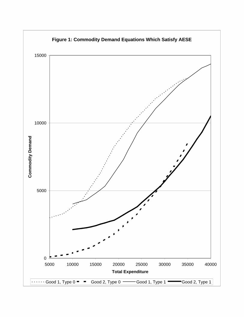
Figure 1: Commodity Demand Equations Which Satisfy AESE

0

5000

10000

15000

5000 10000 15000 20000 25000 30000 35000 40000

Total Expenditure

Co

mm

od

ity

Dem

and

Good 1, Type 0 Good 2, Type 0 Good 1, Type 1 Good 2, Type 1

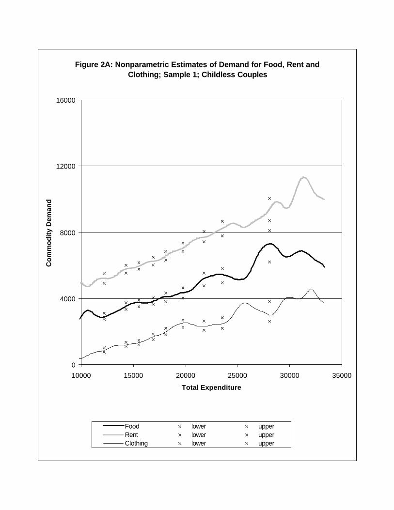
Figure 2A: Nonparametric Estimates of Demand for Food, Rent and Clothing; Sample 1; Childless Couples

0

4000

8000

12000

16000

10000 15000 20000 25000 30000 35000

Total Expenditure

Co

mm

od

ity

Dem

and

Food lower upperRent lower upperClothing lower upper

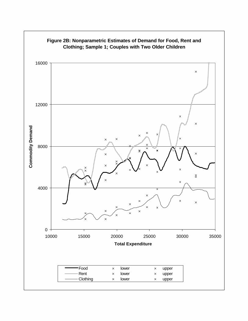
Figure 2B: Nonparametric Estimates of Demand for Food, Rent and Clothing; Sample 1; Couples with Two Older Children

0

4000

8000

12000

16000

10000 15000 20000 25000 30000 35000

Total Expenditure

Co

mm

od

ity

Dem

and

Food lower upperRent lower upperClothing lower upper

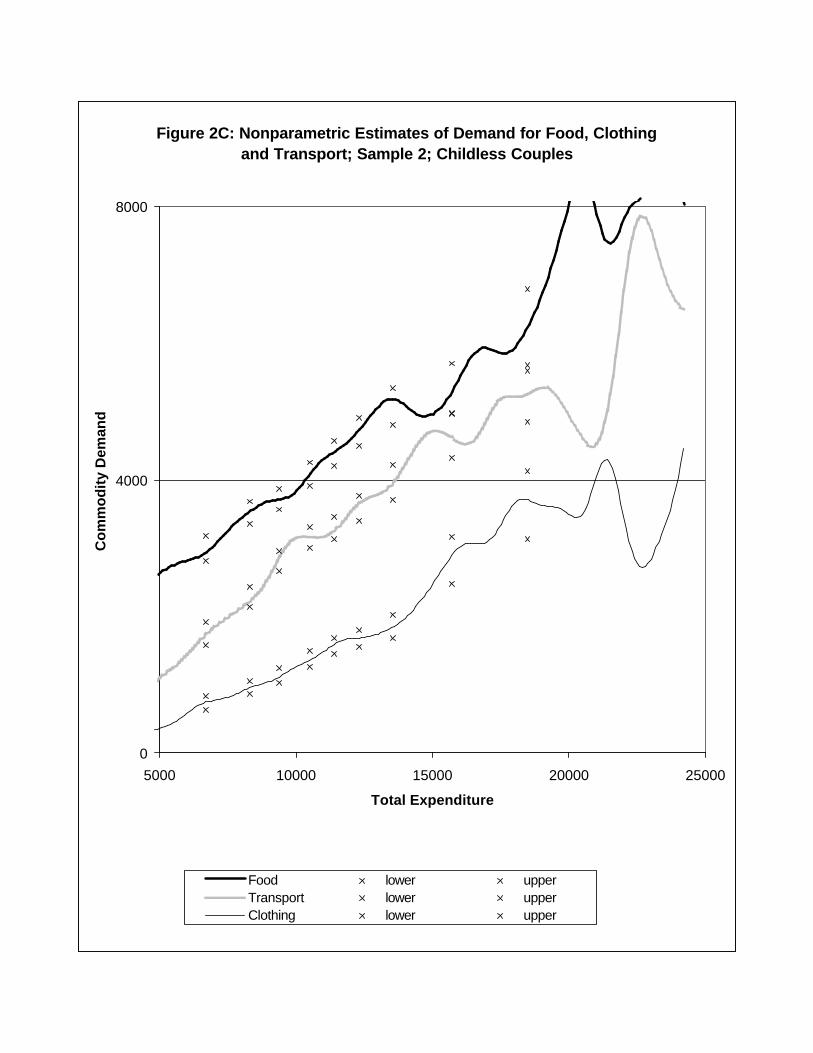
Figure 2C: Nonparametric Estimates of Demand for Food, Clothing and Transport; Sample 2; Childless Couples

0

4000

8000

5000 10000 15000 20000 25000

Total Expenditure

Co

mm

od

ity

Dem

and

Food lower upperTransport lower upperClothing lower upper

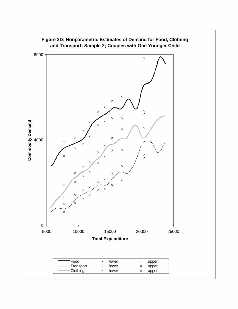
Figure 2D: Nonparametric Estimates of Demand for Food, Clothing and Transport; Sample 2; Couples with One Younger Child

0

4000

8000

5000 10000 15000 20000 25000

Total Expenditure

Co

mm

od

ity

Dem

and

Food lower upperTransport lower upperClothing lower upper