Semiring-based constraint satisfaction and optimization

Semiring-Based Constraint Satisfaction andOptimization

STEFANO BISTARELLI, UGO MONTANARI,AND FRANCESCA ROSSI

University of Pisa, Pisa, Italy

Abstract. We introduce a general framework for constraint satisfaction and optimization whereclassical CSPs, fuzzy CSPs, weighted CSPs, partial constraint satisfaction, and others can be easilycast. The framework is based on a semiring structure, where the set of the semiring specifies thevalues to be associated with each tuple of values of the variable domain, and the two semiringoperations (1 and 3) model constraint projection and combination respectively. Local consistencyalgorithms, as usually used for classical CSPs, can be exploited in this general framework as well,provided that certain conditions on the semiring operations are satisfied. We then show how thisframework can be used to model both old and new constraint solving and optimization schemes, thusallowing one to both formally justify many informally taken choices in existing schemes, and to provethat local consistency techniques can be used also in newly defined schemes.

Categories and Subject Descriptors: I.1.2 [Algebraic Manipulation]: Algorithms—analysis of algo-rithms; I.2.3 [Artificial Intelligence]: Deduction and Theorem Proving—uncertainty; “fuzzy”, andprobabilistic reasoning; I.2.4 [Artificial Intelligence]: Knowledge Representation Formalisms andMethods.

General Terms: Algorithms, Theory.

Additional Key Words and Phrases: Constraint solving, dynamic programming, local consistency,non-crisp constraint reasoning.

1. Introduction

Classical constraint satisfaction problems (CSPs) [Montanari 1974; Mackworth1992] are a very expressive and natural formalism to specify many kinds ofreal-life problems. In fact, problems ranging from map coloring, vision, robotics,job-shop scheduling, VLSI design, etc., can easily be cast as CSPs and solvedusing one of the many techniques that have been developed for such problems orsubclasses of them.1

Authors’ address: Dipartimento di Informatica, Universita di Pisa, Corso Italia 40, 56125 Pisa, Italy,e-mail: {bista,ugo,rossi}@di.unipi.it.Permission to make digital / hard copy of part or all of this work for personal or classroom use isgranted without fee provided that the copies are not made or distributed for profit or commercialadvantage, the copyright notice, the title of the publication, and its date appear, and notice is giventhat copying is by permission of the Association for Computing Machinery (ACM), Inc. To copyotherwise, to republish, to post on servers, or to redistribute to lists, requires prior specific permissionand / or a fee.q 1997 ACM 0004-5411/97/0300-0201 $03.501 See, for example, Freuder [1978; 1988], Mackworth and Freuder [1985], Mackworth [1977], andMontanari [1974].

Journal of the ACM, Vol. 44, No. 2, March 1997, pp. 201–236.

However, they also have evident limitations, mainly due to the fact that theydo not appear to be very flexible when trying to represent real-life scenarioswhere the knowledge is not completely available nor crisp. In fact, in suchsituations, the ability of stating whether an instantiation of values to variables isallowed or not is not enough or sometimes not even possible. For these reasons,it is natural to try to extend the CSP formalism in this direction.

For example, in Rosenfeld et al. [1976], Dubois et al. [1993], and Ruttkay[1994], CSPs have been extended with the ability to associate with each tuple, orto each constraint, a level of preference, and with the possibility of combiningconstraints using min-max operations. This extended formalism has been calledFuzzy CSPs (FCSPs). Other extensions concern the ability to model incompleteknowledge of the real problem [Fargier and Lang 1993], to solve over-con-strained problems [Freuder and Wallace 1992], and to represent cost optimiza-tion problems.

In this paper, we define a constraint solving framework where all suchextensions, as well as classical CSPs, can be cast. However, we do not relax theassumption of a finite domain for the variables of the constraint problems. Themain idea is based on the observation that a semiring (i.e., a domain plus twooperations satisfying certain properties) is all that is needed to describe manyconstraint satisfaction schemes. In fact, the domain of the semiring provides thelevels of consistency (which can be interpreted as cost, or degrees of preference,or probabilities, or others), and the two operations define a way to combineconstraints together. More precisely, we define the notion of constraint solvingover any semiring. Specific choices of the semiring will then give rise to differentinstances of the framework, which may correspond to known or new constraintsolving schemes.

In classical CSPs, so-called local consistency techniques2 have been proved tobe very effective when approximating the solution of a problem. In this paper, westudy how to generalize these techniques to our framework, and we providesufficient conditions over the semiring operations which assure that they can alsobe fruitfully applied to the considered scheme. By “fruitfully applicable,” wemean that (1) the algorithm terminates and (2) the resulting problem isequivalent to the given one and it does not depend on the nondeterministicchoices made during the algorithm. In particular, such conditions rely mainly onhaving an idempotent operator (the 3 operator of the semiring).

The advantage of our framework, that we call SCSP (for Semiring-based CSP),is that one can hopefully see his own constraint solving paradigm as an instanceof SCSP over a certain semiring, and can inherit the results obtained for thegeneral scheme. In particular, one can immediately see whether a local consis-tency technique can be applied. In fact, our sufficient conditions, which arerelated to the chosen semiring, guarantee that the above basic properties of localconsistency hold. Therefore, if they are satisfied, local consistency can safely beapplied. Otherwise, it means that we cannot be sure that in general localconsistency will be meaningful in the chosen instance.

In this paper, we consider several known and new constraint-solving frame-works, casting them as instances of SCSP, and we study the possibility of applying

2 See, for example, Freuder [1978; 1988], Mackworth [1977; 1992], Montanari [1974], and Montanariand Rossi [1986].

202 S. BISTARELLI ET AL.

local consistency algorithms. In particular, we confirm that CSPs enjoy all theproperties needed to use such algorithms, and that they can also be applied toFCSPs. Moreover, we consider probabilistic CSPs [Fargier and Lang 1993], andwe see that local consistency algorithms might be meaningless for such aframework, as well as for weighted CSPs (since the above-cited sufficientconditions do not hold).

We also define a suitable notion of dynamic programming over SCSPs, and weprove that it can be used over any instance of the framework, regardless of theproperties of the semiring. Furthermore, we show that when it is possible toprovide a whole class of SCSPs with parsings trees of bounded size, then theSCSPs of the class can be solved in linear time.

The notion of semiring for constraint solving has been used also in Giacobazziet al. [1992]. However, the use of such a notion is completely different from ours.In fact, in Giacobazzi et al. [1992] the semiring domain (hereby denoted by A) isused to specify the domain of the variables, whereas here we always assume afinite domain (hereby denoted by D) and A is used to model the valuesassociated with the tuples of values of D.

The work which is most related to ours is the one presented in Schiex et al.[1995]. However, the structure they use is not a semiring, but a totally orderedcommutative monoid. This means that the order (to be used to compare differenttuples) is always total, while in our framework it is in general partial, and thismay be useful in some cases, like for example for the instances in Section 7. Also,they associate values with constraints instead of tuples. Moreover, while our aimis to study the properties of the semiring (i.e., mainly the idempotency of 3) thatare sufficient to safely use the local consistency algorithms, they investigate theuse of the values associated with the constraints for deriving useful lower boundsfor branch-and-bound algorithms. Finally, they also study the generalization ofthe property of arc-consistency, and they show that strict monotonicity of theoperator of the monoid guarantees that achieving this generalized notion isNP-complete. Note, however, that one can pass from one formulation to theother by using an appropriate transformation [Bistarelli et al. 1996], but only if atotal order is assumed.

The paper is organized as follows: Section 2 defines c-semirings and theirproperties. Then Section 3 introduces constraint problems over any semiringsand the associated notions of solution and consistency. Then, Section 4 intro-duces the concept of local consistency for SCSPs and gives sufficient conditionsfor the applicability of the local consistency algorithms. Section 5 describes adynamic programming algorithm to solve SCSPs that can be applied to anyinstance of our framework, without any condition. Then, Section 6 studies severalinstances of the SCSP framework and for each of them proves the applicability,or not, of the local consistency algorithms. Section 7 shows that our frameworkallows also for a mixed form of reasoning, where problems are optimizedaccording to several criteria.

This paper is a revised and extended version of Bistarelli et al. [1995]. Themain changes with respect to that paper, apart from the greater level of detailand formalization throughout the whole paper, concern the definition of localconsistency algorithms instead of the less general k-consistency algorithms, themore extensive use of typed locations both for local consistency and for dynamicprogramming, the description of dynamic programming as a particular local

203Semiring-Based Constraint Satisfaction and Optimization

consistency algorithm, and the proof that in some cases (of SCSPs with boundedparsing tree) dynamic programming has a linear complexity.

2. C-Semirings and Their Properties

We extend the classical notion of constraint satisfaction to allow also for (1)noncrisp statements and (2) a more general interpretation of the operations onsuch statements. This allows us to model both classical CSPs and severalextensions of them (like fuzzy CSPs [Dubois et al. 1993; Ruttkay 1994], partialconstraint satisfaction [Freuder and Wallace 1992], etc.), and also to possiblydefine new frameworks for constraint solving. To formally do that, we associate asemiring with the standard notion of constraint problem, so that different choicesof the semiring represent different concrete constraint satisfaction schemes. Infact, such a semiring will give us both the domain for the noncrisp statements andalso the allowed operations on them.

Definition 2.1 (semiring). A semiring is a tuple ^ A, sum, 3, 0, 1& such that

—A is a set and 0, 1 [ A;—sum, called the additive operation, is a commutative (i.e., sum(a, b) 5 sum(b,

a)) and associative (i.e., sum(a, sum(b, c)) 5 sum(sum(a, b), c)) operationsuch that sum(a, 0) 5 a 5 sum(0, a) (i.e., 0 is its unit element);

—3, called the multiplicative operation, is an associative operation such that 1 isits unit element and a 3 0 5 0 5 0 3 a (i.e., 0 is its absorbing element);

—3 distributes over sum (i.e., for any a, b, c [ A, a 3 sum(b, c) 5 sum((a 3b), (a 3 c))).

In the following, we will consider semirings with additional properties of thetwo operations. Such semirings will be called c-semiring, where “c” stands for“constraint”, meaning that they are the natural structures to be used whenhandling constraints.

Definition 2.2 (c-semiring). A c-semiring is a tuple ^ A, 1, 3, 0, 1& such that

—A is a set and 0, 1 [ A;—1 is defined over (possibly infinite) sets of elements of A as follows:3

—for all a [ A, ({a}) 5 a;— (À) 5 0 and ( A) 5 1;— (ø Ai, i [ S) 5 ({ ( Ai), i [ S}) for all sets of indices S (flattening

property).

—3 is a binary, associative and commutative operation such that 1 is its unitelement and 0 is its absorbing element;

—3 distributes over 1 (i.e., for any a [ A and B # A, a 3 (B) 5 ({a 3b, b [ B})).

Operation 1 is defined over any set of elements of A, also over infinite sets.This will be useful later in proving Theorem 2.9. The fact that 1 is defined over

3 When 1 is applied to a two-element set, we will use the symbol 1 in infix notation, while in generalwe will use the symbol in prefix notation.


sets of elements, and not pairs or tuples, automatically makes such an operationcommutative, associative, and idempotent. Moreover, it is possible to show that 0is the unit element of 1; in fact, by using the flattening property we get

({a, 0}) 5 ({a} ø À) 5 ({a}) 5 a. This means that a c-semiring is asemiring (where the sum operation is 1) with some additional properties.

It is also possible to prove that 1 is the absorbing element of 1. In fact, byflattening and by the fact that we set ( A) 5 1, we get ({a, 1}) 5 ({a}ø A) 5 ( A) 5 1.

Let us now consider the advantages of using c-semirings instead of semirings.First, the idempotence of the 1 operation is needed in order to define a partialordering #S over the set A, which will enable us to compare different elementsof the semiring. Such partial order is defined as follows: a #S b iff a 1 b 5 b.Intuitively, a #S b means that b is “better” than a, or, from another point ofview, that, between a and b, the 1 operation chooses b. This ordering will beused later to choose the “best” solution in our constraint problems.

THEOREM 2.3 (#S IS A PARTIAL ORDER). Given any c-semiring S 5 ^ A, 1, 3,0, 1&, consider the relation #S over A such that a #S b iff a 1 b 5 b. Then #S is apartial order.

PROOF. We have to prove that #S is reflexive, transitive, and antisymmetric:

—Since 1 is idempotent, we have that a 1 a 5 a for any a [ A. Thus, bydefinition of #S, we have that a #S a. Thus, #S is reflexive.

—Assume a #S b and b #S c. This means that a 1 b 5 b and b 1 c 5 c.Thus, c 5 b 1 c 5 (a 1 b) 1 c 5 a 1 (b 1 c) 5 a 1 c. Note that herewe also used the associativity of 1. Thus #S is transitive.

—Assume that a #S b and b #S a. This means that a 1 b 5 b and b 1 a 5 a.Thus a 5 b 1 a 5 a 1 b 5 b. Thus, #S is antisymmetric. e

The fact that 0 is the unit element of the additive operation implies that 0 isthe minimum element of the ordering. Thus, for any a [ A, we have 0 #S a.

It is important to notice that both the additive and the multiplicative opera-tions are monotone on such an ordering.

THEOREM 2.4 (1 AND 3 ARE MONOTONE OVER #S). Given any c-semiringS 5 ^ A, 1, 3, 0, 1&, consider the relation #S over A. Then 1 and 3 are monotoneover #S. That is, a #S a9 implies a 1 b #S a9 1 b and a 3 b #S a9 3 b.

PROOF. Assume a #S a9. Then, by definition of #S, a 1 a9 5 a9.Thus, for any b, a9 1 b 5 a 1 a9 1 b. By idempotence of 1, we also have a9

1 b 5 a 1 a9 1 b 5 a 1 a9 1 b 1 b, which, by commutativity of 1, becomesa9 1 b 5 (a 1 b) 1 (a9 1 b). By definition of #S, we have a 1 b #S a9 1b.

Also, from a 1 a9 5 a9 derives that, for any b, a9 3 b 5 (a9 1 a) 3 b 5(by distributiveness) (a9 3 b) 1 (a 3 b). This means that (a 3 b) #S (a9 3b). e

The commutativity of the 3 operation is desirable when such an operation isused to combine several constraints. In fact, were it not commutative, it wouldmean that different orders of the constraints give different results.


Since 1 is also the absorbing element of the additive operation, then a #S 1for all a. Thus, 1 is the maximum element of the partial ordering. This impliesthat the 3 operation is intensive, that is, that a 3 b #S a. This is important sinceit means that combining more constraints leads to a worse (with respect to the#S ordering) result.

THEOREM 2.5 (3 IS INTENSIVE). Given any c-semiring S 5 ^ A, 1, 3, 0, 1&,consider the relation #S over A. Then 3 is intensive, that is, a, b [ A implies a 3 b#S a.

PROOF. Since 1 is the unit element of 3, we have a 5 a 3 1. Also, since 1 isthe absorbing element of 1, we have 1 5 1 1 b. Thus a 5 a 3 (1 1 b). Now,a 3 (1 1 b) 5 {by distributiveness of 3 over 1} (a 3 1) 1 (a 3 b) 5 {1 unitelement of 3} a 1 (a 3 b). Thus, we have a 5 a 1 (a 3 b), which, bydefinition of #S, means that (a 3 b) #S a. e

In the following, we will sometimes need the 3 operation to be closed on acertain finite subset of the c-semiring.

Definition 2.6 ( AD-closed). Given any c-semiring S 5 ^ A, 1, 3, 0, 1&,consider a finite set AD # A. Then 3 is AD-closed if, for any a, b [ AD , (a 3b) [ AD.

We will now show that c-semirings can be assimilated to complete lattices.Moreover, we will also sometimes need to consider c-semirings where 3 isidempotent, which we will show equivalent to distributive lattices. See Davey andPriestly [1990] for a deep treatment of lattices.

Definition 2.7 (lub, glb, lattice, complete lattice [Davey and Priestly 1990]).Consider a partially ordered set S and any subset I of S. Then we define thefollowing:

—an upper bound (resp., lower bound) of I is any element x such that, for all y [I, y # x (resp., x # y);

—the least upper bound (lub) (resp., greatest lower bound (glb)) of I is an upperbound (resp., lower bound) x of I such that, for any other upper bound (resp.,lower bound) x9 of I, we have that x # x9 (resp., x9 # x).

A lattice is a partially ordered set where every subset of two elements has a luband a glb. A complete lattice is a partially ordered set where every subset has alub and a glb.

We will now prove a property of partially ordered sets where every subset hasthe lub, which will be useful in proving that ^ A, #S& is a complete lattice. Noticethat when every subset has the lub, then also the empty set has the lub. Thus, inpartial orders with this property, there is always a global minimum of the partialorder (which is the lub of the empty set).

LEMMA 2.8 (LUB f GLB). Consider a partial order ^ A, #& where there is thelub of every subset I of A. Then there exists the glb of I as well.

PROOF. Consider any set I # A, and let us call LB(I) the set of all lowerbounds of S. That is, LB(I) 5 { x [ A u for all y [ I, x #S y}. Then considera 5 lub(LB(I)). We will prove that a is the glb of I.


Consider any element y [ I. By definition of LB(I), we have that all elementsx in LB(I) are smaller than y, thus y is an upper bound of LB(I). Since a is bydefinition the smallest among the upper bounds of LB(I), we also have that a#S y. This is true for all elements y in I. Thus, a is a lower bound of I, whichmeans that it must be contained in LB(I). Thus, we have found an element of Awhich is the greatest among all lower bounds of I. e

THEOREM 2.9 (^ A, #S& IS A COMPLETE LATTICE). Given a c-semiring S 5 ^ A,1, 3, 0, 1&, consider the partial order #S. Then ^ A, #S& is a complete lattice.

PROOF. To prove that ^ A, #S& is a complete lattice it is enough to show thatevery subset of A has the lub. In fact, by Lemma 2.8, we would get that eachsubset of A has both the lub and the glb, which is exactly the definition of acomplete lattice.

We already know by Theorem 2.3 that ^ A, #S& is a partial order. Now,consider any set I # A, and let us set m 5 sum(I) and n 5 lub(I). Taken anyelement x [ I, we have that x 1 m 5 (by flattening) sum({ x} ø I) 5 sum(I)5 m. Therefore, by definition of #S, we have that x #S m. Thus, also n #S m,since m is an upper bound of I and n by definition is the least among the upperbounds.

On the other hand, we have that m 1 n 5 (by definition of sum) sum({m} ø{n}) 5 (by flattening and since m 5 sum(I)) sum(I ø {n}) 5 (by giving analternative definition of the set I ø {n}) sum(øx[I({ x} ø {n})) 5 (byflattening) sum({sum({ x} ø {n}), x [ I}) 5 (since x #S n and thus sum({ x}ø {n}) 5 n) sum({n}) 5 n. Thus, we have proved that m #S n, which,together with the previous result (that n #S m) yields m 5 n. In other words,we proved that sum(I) 5 lub(I) for any set I # A. Thus, every subset of A, sayI, has a least upper bound (which coincides with sum(I)). Thus, ^ A, #S& is alub-complete partial order. e

Note that the proof of the previous theorem also says that the sum operationcoincides with the lub of the lattice ^ A, #S&.

THEOREM 2.10 (3 IDEMPOTENT IMPLIES ^ A, #S& DISTRIBUTIVE AND 3 5 GLB).Given a c-semiring S 5 ^ A, 1, 3, 0, 1&, consider the corresponding complete lattice^ A, #S&. If 3 is idempotent, then we have that:

(1) 1 distributes over 3;(2) 3 coincides with the glb operation of the lattice;(3) ^ A, #S& is a distributive lattice.

PROOF

(1) (a 1 b) 3 (a 1 c) 5 {since 3 distributes over 1}((a 1 b) 3 a) 1 ((a 1 b) 3 c)) 5 {same as above}((a 3 a) 1 (a 3 b)) 1 ((a 1 b) 3 c)) 5 {by idempotence of 3}(a 1 (a 3 b)) 1 ((a 1 b) 3 c)) 5 {by intensivity of 3 and definition of#S}a 1 ((a 1 b) 3 c)) 5 {since 3 distributes over 1}a 1 ((c 3 a) 1 (c 3 b)) 5 {by intensivity of 3 and definition of #S}a 1 (c 3 b).


(2) Assume that a 3 b 5 c. Then, by intensivity of 3 (see Theorem 2.5), wehave that c #S a and c #S b. Thus, c is a lower bound for a and b. To showthat it is a glb, we need to show that there is no other lower bound c9 suchthat c #s c9. Assume that such c9 exists. We now prove that it must be c9 5c:c9 5 {since c #S c9}c9 1 c 5 {since c 5 a 3 b}c9 1 (a 3 b) 5 {since 1 distributes over 3, see previous point}(c9 1 a) 3 (c9 1 b) 5 {since we assumed c9 #S a and c9 #S b, and bydefinition of 3}a 3 b 5 {by assumption}c.

(3) This comes from the fact that 1 is the lub, 3 is the glb, and 3 distributesover 1 by definition of semiring (the distributiveness in the other direction isgiven by Lemma 6.3 in Davey and Priestly [1990], or can be seen in the firstpoint above). e

Note that, in the particular case in which 3 is idempotent and #S is total, wehave that a 1 b 5 max(a, b) and a 3 b 5 min(a, b).

3. Constraint Systems and Problems

We will now define the notion of constraint system, constraint, and constraintproblem, which will be parametric with respect to the notion of c-semiring justdefined. Intuitively, a constraint system specifies the c-semiring ^ A, 1, 3, 0, 1&to be used, the set of all variables and their domain D.

Definition 3.1 (constraint system). A constraint system is a tuple CS 5 ^S, D,V&, where S is a c-semiring, D is a finite set, and V is an ordered set of variables.

Now, a constraint over a given constraint system specifies the involvedvariables and the “allowed” values for them. More precisely, for each tuple ofvalues (of D) for the involved variables, a corresponding element of A is given.This element can be interpreted as the tuple’s weight, or cost, or level ofconfidence, or else.

Definition 3.2 (constraint). Given a constraint system CS 5 ^S, D, V&,where S 5 ^ A, 1, 3, 0, 1&, a constraint over CS is a pair ^def, con&, where

—con # V, it is called the type of the constraint;—def: Dk 3 A (where k is the cardinality of con) is called the value of the

constraint.

A constraint problem is then just a set of constraints over a given constraintsystem, plus a selected set of variables (thus a type). These are the variables ofinterest in the problem, that is, the variables of which we want to know thepossible assignments compatibly with all the constraints.

Definition 3.3 (constraint problem). Given a constraint system CS 5 ^S, D,V&, a constraint problem P over CS is a pair P 5 ^C, con&, where C is a set ofconstraints over CS and con # V. We also assume that ^def1, con9& [ C and


^def2, con9& [ C implies def1 5 def2. In the following we will write SCSP torefer to such constraint problems.

Note that the above condition (that there are no two constraints with the sametype) is not restrictive. In fact, if in a problem we had two constraints ^def1,con9& and ^def2, con9&, we could replace both of them with a single constraint^def, con9& with def(t) 5 def1(t) 3 def2(t) for any tuple t. Similarly, if C werea multiset, for example, if a constraint ^def, con9& had n occurrences in C, wecould replace all its occurrences with the single constraint ^def9, con9& with

def9~t! 5def~t! 3 · · · 3 def~t!

n times

for any tuple t. However, this assumption implies that the operation of union ofconstraint problems is not just set union, since it has to take into account thepossible presence of constraints with the same type in the problems to becombined (at most one in each problem), and, in that case, it has to perform thejust described constraint replacement operations.

When all variables are of interest, like in many approaches to classical CSP,con contains all the variables involved in any of the constraints of the givenproblem, say P. Such a set, called V(P), is a subset of V that can be recovered bylooking at the variables involved in each constraint. That is, V(P) 5ø ^def,con9&[C con9.

As for classical constraint solving, also SCSPs as defined above can begraphically represented via labeled hypergraphs where nodes are variables,hyperarcs are constraints, and each hyperarc label is the definition of thecorresponding constraint (which can be seen as a set of pairs ^tuple, value&). Thevariables of interest can then be marked in the graph.

Note that the above definition is parametric with respect to the constraintsystem CS and thus with respect to the semiring S. In the following, we willpresent several instantiations of such a framework, and we will show them tocoincide with known and also new constraint satisfaction systems.

In the SCSP framework, the values specified for the tuples of each constraintare used to compute corresponding values for the tuples of values of thevariables in con, according to the semiring operations: the multiplicative opera-tion is used to combine the values of the tuples of each constraint to get thevalue of a tuple for all the variables, and the additive operation is used to obtainthe value of the tuples of the variables in the type of the problem. Moreprecisely, we can define the operations of combination (R) and projection (s)over constraints. Analogous operations have been originally defined for fuzzyrelations in Zadeh [1965], and have then been used for fuzzy CSPs in Dubois etal. [1993]. Our definition is however more general since we do not consider aspecific c-semiring (like that we will define for fuzzy CSPs later) but a generalone.

Definition 3.4 (tuple projection). Given a constraint system CS 5 ^S, D, V&where V is totally ordered via ordering a, consider any k-tuple4 t 5 ^t1, . . . , tk&

4 Given any integer k, a k-tuple is just a tuple of length k. Also, given a set S, an S-tuple is a tuplewith as many elements as the size of S.


of values of D and two sets W 5 {w1, . . . , wk} and W9 5 {w91, . . . , w9m} suchthat W9 # W # V and wi a wj if i # j and w9i a w9j if i # j. Then theprojection of t from W to W9, written t 2W9

W , is defined as the tuple t9 5^t91, . . . , t9m& with t9i 5 t j if w9i 5 wj.

Definition 3.5 (combination). Given a constraint system CS 5 ^S, D, V&,where S 5 ^ A, 1, 3, 0, 1&, and two constraints c1 5 ^def1, con1& and c2 5^def2, con2& over CS, their combination, written c1 R c2, is the constraint c 5^def, con& with

con 5 con1 ø con2

and

def~t! 5 def1~t 2con1

con ! 3 def2~t 2con2

con ! .

Since 3 is both commutative and associative, also R is so. Thus, this operationcan be easily extended to more than two arguments, say C 5 {c1, . . . , cn}, byperforming c1 R c2 R . . . R cn, which we will sometimes denote by (R C).

Definition 3.6 ( projection). Given a constraint system CS 5 ^S, D, V&,where S 5 ^ A, 1, 3, 0, 1&, a constraint c 5 ^def, con& over CS, and a set I ofvariables (I # V), the projection of c over I, written c sI, is the constraint^def9, con9& over CS with

con9 5 I ù con

and

def9~t9! 5 O{t ut2Iùcon

con5t9}

def~t! .

PROPOSITION 3.7. Given a constraint c 5 ^def, con& over a constraint system CSand a set I of variables (I # V), we have that c sI 5 c sIùcon.

PROOF. Follows trivially from Definition 3.6. e

A useful property of the projection operation is the following:

THEOREM 3.8. Given a constraint c over a constraint system CS, we have that csS1

sS25 c sS2

if S2 # S1.

PROOF. To prove the theorem, we have to show that the two constraints c1 5c sS1

sS2and c2 5 c sS2

coincide, that is, they have the same con and thesame def. Assume c 5 ^def, con&, c1 5 ^def1, con1&, and c2 5 ^def2, con2&.Now, con1 5 S2 ù (S1 ù con). Since S2 # S1, we have that con1 5 S2 ù con.Also, con2 5 S2 ù con; thus, con1 5 con2. Consider now def1. By Definition3.6, we have that def1(t1) 5 {t9 ut92S2

S15t1} {t ut2S1con5t9} def(t), which, by

associativity of 1, is the same as {t ut2S2con5t1} def(t), which coincides with

def2(t1) by Definition 3.6. e

We will now prove a property which can be seen as a generalization of thedistributivity property in predicate logic, which we recall is x.( p ` q) 5 ( x.p)` q if x not free in q (where p and q are two predicates). The extension we prove


for our framework is given by the fact that R can be seen as a generalized ` ands as a variant5 of . This property will be useful later in Section 5.

THEOREM 3.9. Given two constraints c1 5 ^def1, con1& and c2 5 ^def2, con2&over a constraint system CS, we have that (c1 R c2) s(con1øcon2)2x 5 c1 scon12x R

c2 if x ù con2 5 À.

PROOF. Let us set c 5 (c1 R c2) s(con1øcon2)2x 5 ^def, con& and c9 5 c1scon12x R c2 5 ^def9, con9& . We will first prove that con 5 con9: con 5(con1 ø con2) 2 x and con9 5 (con1 2 x) ø con2, which is the same as conif x ù con2 5 À, as we assumed. Now we prove that def 5 def9. By definition,def(t) 5 ({t9 ut92con1øcon22x5t}con1øcon2 (def1(t9 2con1

con1øcon2) 3 def2(t9 2con2

con1øcon2)). Now,def2(t9 2con2

con1øcon2) is independent from the summation, since x is not in-volved in c2. Thus, it can be taken out. Also, t9 2con2

con1øcon2 can be substituted byt 2con2

con1øcon2, since t9 and t must coincide on the variables different from x.Thus, we have: (({t9ut92con1øcon22x5t}con1øcon2 def1(t9 2con1

con1øcon2)) 3 def2(t 2con2

con1øcon22x). Now,the summation is done over those tuples t9 that involve all the variables and coincidewith t on the variables different from x. By observing that the elements of thesummation are given by def1(t9 2con1

con1øcon2), and thus they only contain variables incon1, we can conclude that the result of the summation does not change if it is doneover the tuples involving only the variables in con1 and still coinciding with t over thevariables in con1 that are different from x. Thus, we get:

S O{t1ut12con12xcon1 5t2con12x

con1øcon22x} def1~t1!D 3 def2~t 2con2

con1øcon22x! .

It is easy to see that this formula is exactly the definition of def9. e

Using the operations of combination and projection, we can now define thenotion of solution of an SCSP. In the following, we will consider a fixedconstraint system CS 5 ^S, D, V&, where S 5 ^ A, 1, 3, 0, 1&.

Definition 3.10 (solution). Given a constraint problem P 5 ^C, con& over aconstraint system CS, the solution of P is a constraint defined as Sol(P) 5 (RC) scon.

In words, the solution of an SCSP is the constraint induced on the variables incon by the whole problem. Such a constraint provides, for each tuple of values ofD for the variables in con, a corresponding value of A. Sometimes, it is enoughto know just the best value associated with such tuples. In our framework, this isstill a constraint (over an empty set of variables), and will be called the best levelof consistency of the whole problem, where the meaning of “best” depends onthe ordering #S defined by the additive operation.

Definition 3.11 (best level of consistency). Given an SCSP problem P 5 ^C,con&, we define blevel(P) [ S such that ^blevel(P), À& 5 (R C) sÀ. Moreover,we say that P is consistent if 0 ,S blevel(P), and that P is a-consistent ifblevel(P) 5 a.

5 Note however that the operator corresponding to x is given by sW2{ x}W .


Informally, the best level of consistency gives us an idea of how much we cansatisfy the constraints of the given problem. Note that blevel(P) does not dependon the choice of the distinguished variables, due to the associative property ofthe additive operation. Thus, since a constraint problem is just a set ofconstraints plus a set of distinguished variables, we can also apply function blevelto a set of constraints only. More precisely, blevel(C) will mean blevel(^C, con&)for any con.

Note that blevel(P) can also be obtained by first computing the solution andthen projecting such a constraint over the empty set of variables, as the followingproposition shows.

PROPOSITION 3.12. Given an SCSP problem P, we have that Sol(P) sÀ 5^blevel(P), À&.

PROOF. Sol(P) sÀ coincides with ((R C) scon) sÀ by definition ofSol(P). This coincides with (R C) sÀ by Theorem 3.8, thus it is the same as^blevel(P), À& by Definition 3.11. e

Another interesting notion of solution, more abstract than the one definedabove, but sufficient for many purposes, is the one that does not consider thosetuples whose associated value is worse (with respect to #S) than that of othertuples.

Definition 3.13 (abstract solution). Given an SCSP problem P 5 ^C, con&,consider Sol(P) 5 ^def, con&. Then the abstract solution of P is the setASol(P) 5 {^t, v& u def(t) 5 v and there is no t9 such that v #S def(t9)}.

Note that, when the #S ordering is a total order (i.e., when, for any a and b,a 1 b is either a or b), then the abstract solution contains only those tupleswhose associated value coincides with blevel(P). In general, instead, an incompa-rable set of tuples is obtained, and thus blevel(P) is just an upper bound of thevalues associated with the tuples.

By using the ordering #S over the semiring, we can also define a correspond-ing ordering on constraints with the same type.

Definition 3.14 (constraint ordering). Consider two constraints c1, c2 overCS, and assume that con1 5 con2 and ucon1u 5 k. Then c1 vS c2 if and only if,for all k-tuples t of values from D, def1(t) #S def2(t).

Notice that, if c1 vS c2 and c2 vS c1, then c1 5 c2.

THEOREM 3.15 (vS IS A PARTIAL ORDER). The relation vS over the set ofconstraints over CS is a partial order.

PROOF. By definition, such a relation is antisymmetric. Also, it is easy to seethat it is reflexive and transitive. e

The notion of constraint ordering, and the fact that the solution is a constraint,can also be useful to define an ordering on problems.

Definition 3.16 ( problem ordering and equivalence). Consider two SCSP prob-lems P1 5 ^C1, con& and P2 5 ^C2, con& over CS. Then P1 vP P2 if Sol(P1)vS Sol(P2). If P1 vP P2 and P2 vP P1, then they have the same solution. Thus,we say that P1 and P2 are equivalent and we write P1 [ P2.


THEOREM 3.17 (vP IS A PREORDER AND [ IS AN EQUIVALENCE). The relationvP over the set of constraint problems over CS is a preorder. Moreover, [ is anequivalence relation.

PROOF. It is trivial to see that vP is reflexive and transitive, due to thedefinition of constraint ordering vS. Thus, vP is a preorder. From this, it derivesthat [ is reflexive and transitive as well. Moreover, it is trivially symmetric. e

The ordering vP can also be used for ordering sets of constraints, since a set ofconstraint is just a problem where con contains all the variables.

It is interesting now to note that, as in the classical CSP case, also the SCSPframework is monotone. That is, if some constraints are added, the solution ofthe new problem precedes that of the old one in the ordering vS. In other words,the new problem precedes the old one with respect to the preorder vP.

THEOREM 3.18 (MONOTONICITY). Consider two SCSP problems P1 5 ^C1, con&and P2 5 ^C1 ø C2, con& over CS. Then P2 vP P1 and blevel(P2) #S blevel(P1).

PROOF. P2 vP P1 follows from the intensivity of 3 and the monotonicity of1. The same holds also for blevel(P2) #S blevel(P1), since both Sol andblevel(P) are obtained by projecting over a subset of the variables (which isalways empty in the case of blevel(P)). e

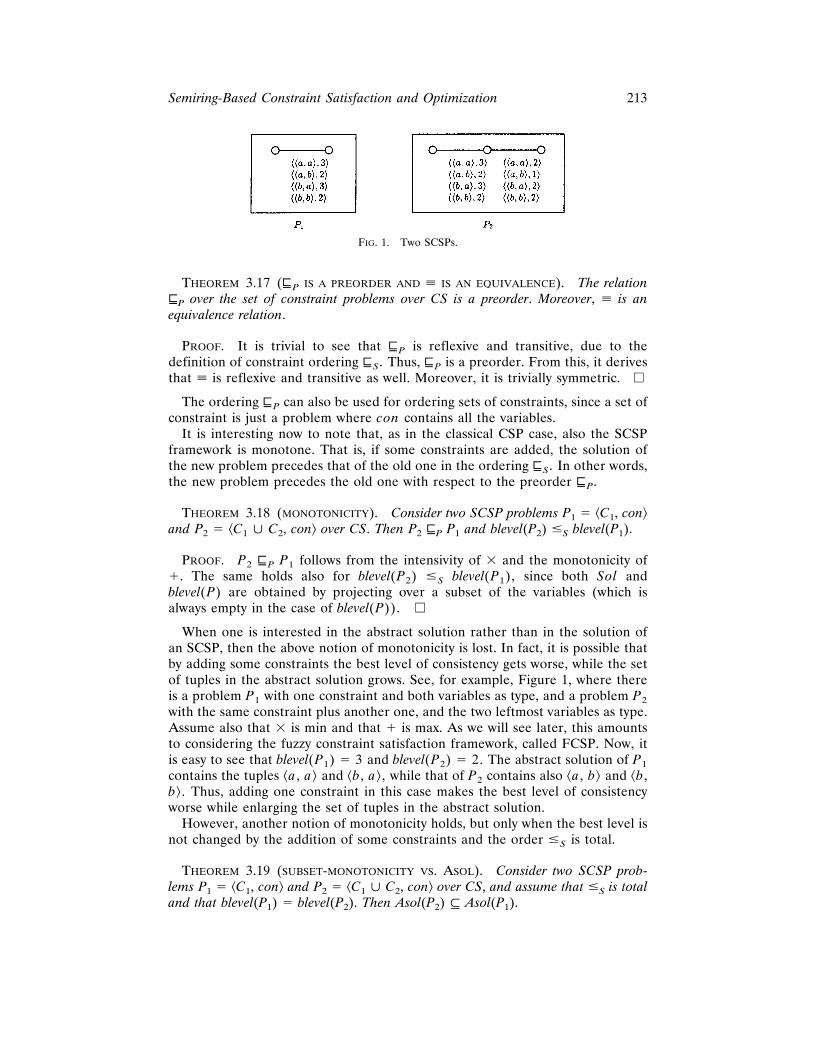
When one is interested in the abstract solution rather than in the solution ofan SCSP, then the above notion of monotonicity is lost. In fact, it is possible thatby adding some constraints the best level of consistency gets worse, while the setof tuples in the abstract solution grows. See, for example, Figure 1, where thereis a problem P1 with one constraint and both variables as type, and a problem P2with the same constraint plus another one, and the two leftmost variables as type.Assume also that 3 is min and that 1 is max. As we will see later, this amountsto considering the fuzzy constraint satisfaction framework, called FCSP. Now, itis easy to see that blevel(P1) 5 3 and blevel(P2) 5 2. The abstract solution of P1contains the tuples â, a& and ^b, a&, while that of P2 contains also â, b& and ^b,b&. Thus, adding one constraint in this case makes the best level of consistencyworse while enlarging the set of tuples in the abstract solution.

However, another notion of monotonicity holds, but only when the best level isnot changed by the addition of some constraints and the order #S is total.

THEOREM 3.19 (SUBSET-MONOTONICITY VS. ASOL). Consider two SCSP prob-lems P1 5 ^C1, con& and P2 5 ^C1 ø C2, con& over CS, and assume that #S is totaland that blevel(P1) 5 blevel(P2). Then Asol(P2) # Asol(P1).

FIG. 1. Two SCSPs.


PROOF. If #S is total, then the abstract solution is a set of tuples withassociated value exactly the best level. Take a tuple t in ASol(P2). This meansthat the value associated with t in P2 is blevel(P2). Then, by Theorem 3.18, thevalue associated with t in P1, say v, is such that blevel(P2) #S v. By assumption,blevel(P1) 5 blevel(P2). If v Þ blevel(P2), then this assumption is violated.Thus, it must be v 5 blevel(P2) 5 blevel(P1). Thus, t is also in Asol(P1).Therefore, Asol(P2) # Asol(P1). e

4. Local Consistency

Computing any one of the previously defined notions (the best level of consis-tency, the solution, and the abstract solution) is an NP-hard problem. Thus, itcan be convenient in many cases to approximate such notions. In classical CSPs,this is done using the so-called local consistency techniques.6 The main idea is tochoose some subproblems in which to eliminate local inconsistency, and theniterate such elimination in all the chosen subproblems until stability. The mostwidely known local consistency algorithms are arc-consistency [Mackworth 1977],where subproblems contain just one constraint, and path-consistency [Montanari1974], where subproblems are triangles (i.e., they are complete binary graphsover three variables). The concept of k-consistency [Freuder 1978], wheresubproblems contain all constraints among subsets of k chosen variables, gener-alizes them both. However, all subproblems are of the same size (which is k). Ingeneral, one may imagine several algorithms where instead the consideredsubparts of the SCSP have different sizes. This generalization of the k-consis-tency algorithms has been described in Montanari and Rossi [1991] for classicalCSPs. Here we follow the same approach as in Montanari and Rossi [1991], butwe extend the definitions and results presented there to the SCSP framework,and we show that all the properties still hold, provided that certain properties ofthe semiring are satisfied.

Applying a local consistency algorithm to a constraint problem means explici-tating some implicit constraints, thus possibly discovering inconsistency at a locallevel. In classical CSPs, this is crucial, since local inconsistency implies globalinconsistency. We will now show that such a property holds also for SCSPs.

DEFINITION 4.1 (LOCAL INCONSISTENCY). Consider an SCSP problem P 5 ^C,con&. Then we say that P is locally inconsistent if there exists C9 # C such thatblevel(C9) 5 0.

THEOREM 4.2 (NECESSITY OF LOCAL CONSISTENCY). Consider an SCSP prob-lem P which is locally inconsistent. Then it is not consistent.

PROOF. We have to prove that blevel(P) 5 0. We know that P is locallyinconsistent. That is, there exists C9 # C such that blevel(C9) 5 0. By Theorem3.18, we have that blevel(P) #S blevel(C9); thus, blevel(P) #S 0. Since 0 is theminimum in the ordering #S, then we immediately have that blevel(P) must be 0as well. e

In the SCSP framework, we can be even more precise, and relate the best levelof consistency of the whole problem (or, equivalently, of the set of all its

6 See, for example, Freuder [1978; 1988], Kumar [1992], and Montanari and Rossi [1991].


constraints) to that of its subproblems, even though such level is not 0. In fact, itis possible to prove that if a problem is a-consistent, then all its subproblems areb-consistent, where a #S b.

THEOREM 4.3. (LOCAL AND GLOBAL A-CONSISTENCY). Consider a set of con-straints C over CS, and any subset C9 of C. If C is a-consistent, then C9 isb-consistent, with a #S b.

PROOF. The proof is similar to the previous one. If C is a-consistent, itmeans, by definition, that blevel(C) 5 a. Now, if we take any subset C9 of C, byTheorem 3.18 we have that blevel(C) #S blevel(C9). Thus, a #S blevel(C9). e

In order to define the subproblems to be considered by a local consistencyalgorithm, we use the notion of local consistency rule. The application of such arule consists of solving one of the chosen subproblems. To model this, we needthe additional notion of typed location. Informally, a typed location is just alocation l (as in ordinary store-based programming languages) which has a set ofvariables con as type, and thus can only be assigned a constraint c 5 ^def, con&with the same type. In the following, we assume to have a location for every setof variables, and thus we identify a location with its type. Note that at any stageof the computation the store will contain a constraint problem with only a finitenumber of constraints, and thus the relevant locations will always be finitelymany.

Definition 4.4 (typed location). A typed location l is a set of variables.

Definition 4.5 (value of a location). Given a CSP P 5 ^C, con&, the value[l]P of the location l in P is defined as the constraint ^def, l& [ C if it exists, as^1, l& otherwise. Given n locations l1, . . . , ln, the value [{l1, . . . , ln}]P of thisset of locations in P is defined instead as the set of constraints {[ l1]P, . . . ,[ln]P}.

Definition 4.6 (assignment). An assignment is a pair l :5 c where c 5 ^def,l&. Given a CSP P 5 ^C, con&, the result of the assignment l :5 c is the problem[l :5 c](P) defined as:

@l :5 c#~P! 5 ^$^def9 , con9& [ C u con9 Þ l% ø c, con& .

Thus, an assignment l :5 c is seen as a function from constraint problems toconstraint problems, which modifies a given problem by changing just oneconstraint, the one with type l. The change consists in replacing such a constraintwith c. If there is no constraint of type l, then constraint c is added to the givenproblem.

Definition 4.7 (local consistency rule). Given an SCSP P 5 ^C, con&, a localconsistency rule r for P is defined as r 5 l 4 L, where L is a set of locations, lis a location, and l [y L.

Applying r to P means assigning to location l the constraint obtained by solvingthe subproblem of P containing the constraints specified by the locations in L ø{l}.

Definition 4.8 (rule application). Given a local consistency rule r 5 l 4 Land a constraint problem P, the result of applying r to P is


@l4 L#~P! 5 @l :5 Sol~^@L ø $l%#P, l&!#~P! .

Since a rule application is defined as a function from problems to problems, theapplication of a sequence S of rules to a problem is easily provided by functioncomposition. Thus, we have that [r1; S](P) 5 [S]([r1](P)).

Notice for example that [l 4 À](P) 5 P.

THEOREM 4.9 (EQUIVALENCE FOR RULES). Given an SCSP P and a rule r forP, we have that P [ [r](P) if 3 is idempotent.

PROOF. Assume that P 5 ^C, con&, and let r 5 l 4 L. Then we have P9 5[l 4 L](P) 5 [l :5 Sol(^[L ø {l}]P, l&)](P) 5 ^{^def9, con9& [ C u con9 Þl} ø Sol(^[L ø {l}]P, l&), con&. Let now C(r) 5 [L ø {l}]P, and C9 5 C 2C(r). Then P contains the constraints in the set C9 ø C(r), while P9 containsthe constraints in C9 ø (C(r) 2 c) ø ((R C(r)) s l), where c 5 ^def, l& 5[l]P. In fact, by definition of solution, Sol(^[L ø {l}]P, l&) can be written as (RC(r)) s l. Since the set C9 is present in both P and P9, we will not consider it,and we will instead prove that the constraint cpre 5 R C(r) coincides with cpost 5(R(C(r) 2 {c})) R ((R C(r)) s l). In fact, if this is so, then P [ P9.

First of all, it is easy to see that cpre and cpost have the same type ø(L ø {l}).Let us now consider the definitions of such two constraints. Let us set ci 5 [l i]P

5 ^defi, l i& for all l i [ L, and assume L 5 {l1, . . . , ln}. Thus, C(r) 5 {c,c1, . . . , cn}. We have that, taken any tuple t of length uø(L ø {l}) u, defpre(t)5 def(t 2 l) 3 () i defi(t 2 l i

)), while defpost(t) 5 () i defi(t 2 l i)) 3

t9 ut92 l5t2 l(def(t9 2 l) 3 () i defi(t9 2 l i

))). Now, since the sum is done overall t9 such that t9 2 l 5 t 2 l, we have that def(t9 2 l) 5 def(t 2 l). Thus, def(t92 l) can be taken out from the sum since it appears the same in each factor.Thus, we have defpost(t) 5 () i defi(t 2 l i

)) 3 def(t 2 l) 3 t9 ut92 l5t2 l() i

defi(t9 2 l i)). Consider now t9 ut92 l5t2 l

() i defi(t9 2 l i)): one of the t9 such that

t9 2 l 5 t 2 l must be equal to t. Thus, the sum can be written also as () i defi(t2 l i

) 1 t9 ut92 l5t2 l,t9Þt () i defi(t9 2 l i)). Thus, we have defpost(t) 5 () i defi(t

2 l i)) 3 def(t 2 l) 3 () i defi(t 2 l i

) 1 t9 ut92 l5t2 l,t9Þt () i defi(t9 2 l i))).

Let us now consider any two elements a and b of the semiring. Then it is easyto see that a 3 (a 1 b) 5 a. In fact, by intensivity of 3 (see Theorem 2.5), wehave that a 3 c #S a for any c. Thus, if we choose c 5 a 1 b, a 3 (a 1 b) #S

a. On the other hand, since a 1 b is the lub of a and b, we have that a 1 b $S

a. Thus, by monotonicity of 3, we have a 3 (a 1 b) $S a 3 a. Now, since weassume that 3 is idempotent, we have that a 3 a 5 a, thus a 3 (a 1 b) $S a.Therefore, a 3 (a 1 b) 5 a. This result can be used in our formula for defpost

(t), by setting a 5 () i defi(t 2 l i)) and b 5 t9 ut9 2 l5t2 l,t9Þt () i defi(t9 2 l i

)).In fact, by replacing a 3 (a 1 b) with a, we get defpost(t) 5 () i defi(t 2 l i

)) 3def(t 2 l), which coincides with defpre(t). e

Definition 4.10 (stable problem). Given an SCSP problem P and a set R oflocal consistency rules for P, P is said to be stable with respect to R if, for eachr [ R, [r](P) 5 P.

A local consistency algorithm consists of the application of several rules to thesame problem, until stability of the problem with respect to all the rules. At each


step of the algorithm, only one rule is applied. Thus, the rules will be applied ina certain order, which we call a strategy.

Definition 4.11 (strategy). Given a set R of local consistency rules for anSCSP, a strategy for R is an infinite sequence S [ R`. A strategy S is fair if eachrule of R occurs in S infinitely often.

Definition 4.12 (local consistency algorithm). Given an SCSP problem P, a setR of local consistency rules for P, and a fair strategy S for R, a local consistencyalgorithm applies to P the rules in R in the order given by S. Thus, if the strategyis S 5 s1s2s3

. . . , the resulting problem is

P9 5 @s1; s2; s3; · · ·#~P!

The algorithm stops when the current SCSP is stable with respect to R.

Note that this formulation of local consistency algorithms extends the usualone for k-consistency algorithms [Freuder 1978], which can be seen as localconsistency algorithms where all rules in R are of the form l 4 L, where L 5{l1, . . . , ln} and uø i51, . . . ,nliu 5 ul u 5 k 2 1. That is, exactly k 2 1 variablesare involved in the locations7 in L.

When a local consistency algorithm terminates,8 the result is a new problemwhich has the graph structure of the initial one plus possibly new arcs represent-ing newly introduced constraints (we recall that constraints posing no restrictionson the involved variables are usually not represented in the graph structure), butwhere the definition of some of the constraints has been changed. Moreprecisely, assume R 5 {r1, . . . , rn}, and ri 5 l i 4 Li for all i 5 1, . . . , n.Then the algorithm uses, among others, n typed locations l i of type coni. Assumealso that each of such typed locations has value defi when the algorithmterminates. Consider also the set of constraints C(R) which have type coni. Thatis, C(R) 5 {^def, con& such that con 5 coni for some i between 1 and n}.Informally, these are the constraints that may have been modified (via the typedlocation mechanism) by the algorithm. Then, if the initial SCSP is P 5 ^C, con&,the resulting SCSP is P9 5 local-cons(P, R, S) 5 ^C9, con&, where C9 5 C 2C(R) ø (ø i51, . . . ,n ^defi, coni&).

In classical CSPs, any local consistency algorithm enjoys some importantproperties. We now will study these same properties in the SCSP framework, andpoint out the corresponding properties of the semiring operations which aresufficient for them to hold. The desired properties are as follows:

(1) any local consistency algorithm returns a problem which is equivalent to thegiven one;

(2) any local consistency algorithm terminates in a finite number of steps;(3) the strategy, if fair, used in a local consistency algorithm does not influence

the resulting problem.

THEOREM 4.13 (EQUIVALENCE). Consider an SCSP P and the problem P9 5local-cons(P, R, S). Then P [ P9 if the multiplicative operation of the semiring (3)is idempotent.

7 We recall that locations are just sets of variables.8 We will consider the termination issue later.


PROOF. By Definition 4.12, a local consistency algorithm is just a sequence ofapplications of local consistency rules. Since, by Theorem 4.9, we know that eachrule application returns an equivalent problem, by induction we can concludethat the problem obtained at the end of a local consistency algorithm isequivalent to the given one. e

THEOREM 4.14 (TERMINATION). Consider any SCSP P 5 ^C, con& over theconstraint system CS 5 ^S, D, V& and the set AD 5 ø^def, con&[C R(def ), whereR(def ) 5 {a u t with def(t) 5 a}. Then the application of a local consistencyalgorithm to P terminates in a finite number of steps if AD is contained in a set Iwhich is finite and such that 1 and 3 are I-closed.

PROOF. Each step of a local consistency algorithm may change the definitionof one constraint by assigning a different value to some of its tuples. Such valueis strictly worse (in terms of #S) since 3 is intensive. Moreover, it can be a valuewhich is not in AD but in I 2 AD . If the state of the computation consists of thedefinitions of all constraints, then at each step we get a strictly worse state (interms of vS). The sequence of such computation states, until stability, has finitelength, since by assumption I is finite and thus the value associated with eachtuple of each constraint may be changed at most uI u times. e

An interesting special case of the above theorem occurs when the chosensemiring has a finite domain A. In fact, in that case the hypotheses of thetheorem hold with I 5 A.

COROLLARY 4.15. Consider any SCSP problem P over the constraint systemCS 5 ^S, D, V&, where S 5 ^ A, 1, 3, 0, 1&, and A is finite. Then the application ofa local consistency algorithm to P terminates in a finite number of steps.

We will now prove that, if 3 is idempotent, no matter which strategy is usedduring a local consistency algorithm, the result is always the same problem.

THEOREM 4.16 (ORDER-INDEPENDENCE). Consider an SCSP problem P andtwo different applications of the same local consistency algorithm to P, producingrespectively the SCSPs P9 5 local-cons(P, R, S) and P0 5 local-cons(P, R, S9). ThenP9 5 P0 if the multiplicative operation of the semiring (3) is idempotent.

PROOF. Each step of the local consistency algorithm, which applies one of thelocal consistency rules in R, say r, has been defined as the application of afunction [r] that takes an SCSP problem P and returns another problem P9 5[r](P), and that may change the definition of the constraint connecting thevariables in l (if the applied rule is r 5 l 4 L). Thus, the whole algorithm maybe seen as the repetitive application of the functions [r], for all r [ R, until nomore change can be done. If we can prove that each [r] is a closure operator[Davey and Priestly 1990], then classical results on chaotic iteration [Cousot1977] allow us to conclude that the problem resulting from the whole algorithmdoes not depend on the order in which such functions are applied. Closureoperators are just functions, which are idempotent, monotone, and intensive. Wewill now prove that each [r] enjoys such properties. We remind that [r] justcombines a constraint with the combination of other constraints.

If 3 is idempotent, then [r] is idempotent as well, that is, [r]([r](P)) 5 [r](P)for any P. In fact, combining the same constraint more than once does not


change the problem by idempotency of 3. Also, the monotonicity of 3 (seeTheorem 2.4) implies that of [r], that is, P v P9 implies [r](P) v [r](P9). Notethat, although v has been defined only between constraints, here we use itamong constraint problems, meaning that such a relationship holds among eachpair of corresponding constraints in P and P9. Finally, the intensivity of 3implies that [r] is intensive as well, that is, [r](P) v P. In fact, P and [r](P) justdiffer in one constraint, which, in [r](P), is just the corresponding constraint ofP combined with some other constraints. e

Note that the above theorems require that 3 is idempotent for a localconsistency algorithm to be meaningful. However, there is no requirement overthe nature of #S. More precisely, #S can be partial. This means that thesemiring operations 1 and 3 can be different from max and min respectively(see note at the end of Section 2).

Note also that, by definition of rule application, constraint definitions arechanged by a local consistency algorithm in a very specific way. In fact, even inthe general case in which the ordering #S is partial, the new values assigned totuples are always smaller than or equal to the old ones in the partial order. Inother words, local consistency algorithms do not “jump” in the partially orderedstructure from one value to another one which is unrelated to the first one. Moreprecisely, the following theorem holds.

THEOREM 4.17 (LOCAL CONSISTENCY AND PARTIAL ORDERS). Given an SCSPproblem P, consider any value v assigned to a tuple in a constraint of such problem.Also, given any set R of local consistency rules and strategy S, consider P9 5local-cons(P, R, S), and the value v9 assigned to the same tuple of the sameconstraint in P9. Then we have that v9 #S v.

PROOF. By definition of rule application (see Definition 4.8), the formuladefining the new value associated to a tuple of a constraint can be assimilated to(v 3 a) 1 (v 3 b), where v is the old value for that tuple and a and b arecombinations of values for tuples of other constraints in the graph of the rule.Now, we have (v 3 a) 1 (v 3 b) 5 v 1 (a 3 b) by distributivity of 1 over 3(see Theorem 2.10). Also, (v 3 c) #S v for any c by intensivity of 3 (seeTheorem 2.5), thus v 1 (a 3 b) #S v. e

One could imagine other generalizations with the same desired properties asthe ones proved above (i.e., termination, equivalence, and order-independence).For example, one could design an algorithm that avoids (or compensates) theeffect of cumulation coming from a nonidempotent 3. Or also, one couldgeneralize the equivalence property, by allowing the algorithm to return anon-equivalent problem (but however being in a certain relationship with theoriginal problem). Finally, the order-independence property states that any orderis fine, as far as the resulting problem is concerned. Another desirable property,related to this, could be the existence of an ordering which makes the algorithmbelong to a specific complexity class.

5. Dynamic Programming

Dynamic programming [Bellman 1997; Bellman and Dreyfus 1962] can be usedto solve a problem by solving some subproblems of it and then combining their


solutions to obtain the solution of the whole problem (see, e.g., Gnesi et al.[1981] for its use in graphs and Montanari and Rossi [1986] for its adoption inclassical CSPs). In the SCSP framework, a suitably instantiated version ofdynamic programming can be fruitfully used as well: at each step, a subset ofconstraints is chosen and solved, and its solution (which, we recall, is aconstraint) replaces the whole subset of constraints.

Before defining the algorithm, we need to describe in a tree-like way the SCSPto be solved, so that the algorithm can then follow the tree structure in abottom-up way.

Definition 5.1 ( parsing tree). Given an SCSP P 5 ^C, con&, a parsing tree ofP is a sequence of local consistency rules S 5 r1; . . . ; rn, where ri 5 (l i 4 Li).Let

—L 5 {l i, i 5 1, . . . , n} ø ø i51, . . . ,n Li (i.e., L is the set of all locationsoccurring in all rules in S);

—l i a l iff l [ Li (i.e., rule ri “generates” location l );—l i a v iff v [y l i and v [ l9 with l9 [ Li (i.e., rule ri “generates” variable v);—for any x location or variable, prec( x) 5 {l ul a x}.

Then we require that

—(tree-like) for any x variable or location, if x 5 ln or x [ ln, then prec( x) 5 À,else prec( x) is a singleton;

—(cover) con 5 ln, and ^def, con9& [ C implies con9 [ L;—(bottom-up parsing) l i a l j implies j , i.

In words, the above definition provides a sequence of rules that cover thewhole problem and are connected among them as a tree. Moreover, the sequencegives a bottom-up visit of the tree. It is now easy to define a dynamicprogramming algorithm where, at each step, one rule is processed, according tothe given sequence.

Definition 5.2 (dynamic programming algorithm). Given an SCSP P, con-sider a parsing tree S 5 r1; . . . ; rn of P. Then compute [S](P).

We will now prove that the value of location ln when the algorithm terminatescoincides with the solution of the given problem P.

THEOREM 5.3 (SOLUTION). Given an SCSP P 5 ^C, l& and a parsing tree S forP, we have that Sol(P) 5 [l][S](P).

PROOF. We will prove the statement of the theorem by induction on thelength of the parsing tree. For the base case, consider a parsing tree with just onerule, that is, l 4 L. It is easy to see that [ l][r](P) is the solution of P. In fact,applying this rule means exactly solving the whole problem. Assume now that thestatement holds for all parsings with n 2 1 rules, and consider a parsing S1 withn rules r1, . . . , rn, where ri 5 l i 4 Li for all i 5 1, . . . , n. Consider now thefirst rule of this parsing, that is, r1 5 l1 4 L1, and take another rule ri such thatl1 5 l i or l1 [ Li, and there is no other rule rj with j , i and such that l1 5 l j

or l1 [ Lj. That is, ri is the first rule after r1 which has l1 either in its left-handside or in its right-hand side. Note that such rule must exist by definition of


parsing tree. In fact, either l1 5 ln, and in this case l1 must appear at least in theleft hand side on rn, or l1 Þ ln, in which case it must be generated by one rule(ri). We will consider now the two separate cases: that l1 5 l i and that l1 [ Li.

Assume that l1 [ Li. Consider then the sequence S2 5 r2, . . . , ri21, r1,ri, . . . , rn. It is easy to see that this is still a parsing for the given problem.Moreover, the constraint of type ln resulting after applying the rules in S2coincides with that obtained after applying the rules in S1. In fact, since l1 can begenerated by just one rule (by definition of parsing), all rules in {r2, . . . , ri21}cannot change the definition of l1 and thus applying r1 before or after themcannot change the resulting constraint. Consider now another sequence S3 ofn 2 1 rules r2, . . . , ri21, r9i, ri11, . . . , rn, where r9i 5 l i 4 Li ø L1. It is easyto see that this sequence of rules is again a parsing tree for P, thus by inductionhypothesis the constraint with type ln after the application of S2 is the solution ofthe problem. Now we have to show that such a constraint coincides with thatobtained at location ln after applying sequence S2 (which we already know tocoincide with that obtained at location ln after sequence S1). What makes S2 andS3 differ is the fact that rule r1 of S2 has been “merged” with rule ri to give ruler9i in S3. More precisely, the application of rule r9i combines all constraintsspecified by L1 ø Li, while the application of first rule r1 and then rule ri

combines first the constraint specified by L1 and then combines the resultingconstraint with those constraints specified by Li. We will show that these twomethods yield the same final constraint.

In this proof, for ease of readability, we will write l instead of [l]P. On one side(rule r9i) we have the constraint (R(Li ø L1 ø {l i})) s l i

, and on the other side(rule r1 and then ri) we have the constraint (R((Li 2 {l1}) ø {l i} ø {(R(L1ø {l1})) s l1

})) s l i. Thus, we have to prove that:

~ ^ ~Li ø L1 ø $l i%!! s l i5

~ ^ ~~Li 2 $l1%! ø $l i% ø $~ ^ L1 ø $l1%! s l1%!! s l i

.

We will start from the left-hand side of the formula and try to reach theright-hand side. We have:

(R(Li ø L1 ø {l i})) s l i5

{by separating (Li ø {l i}) 2 {l1} and L1 ø {l1} which are disjoint}

((R((Li ø {l i}) 2 {l1}))R(R(L1 ø {l1}))) s l i5

{by Theorem 3.8, and letting Vi 5 ø(Li ø {l i}), that is the set of all variablesinvolved in rule ri}

((R((Li ø {l i}) 2 {l1}))R(R(L1 ø {l1}))) sVis l i

5

{by Theorem 3.9, since the variables not in Vi are not involved in Li ø {l i} 2{l1}}

((R((Li ø {l i}) 2 {l1}))R(R(L1 ø {l1}) sVi)) s l i

5

{by Proposition 3.7, since Vi ù V1 5 l1, where V1 5 (ø L1) ø l1}

((R((Li ø {l i}) 2 {l1}))R(R(L1 ø {l1})) s l1) s l i


which coincides with the right hand side of the formula.

Let us now consider the second case, in which l1 5 l i. Then consider thesequence S2 5 r2, . . . , ri21, r1, ri, . . . , rn. With a reasoning similar to above, itis easy to see that S2 is still a parsing tree for P and that the constraint of type ln

obtained via S2 is the same as the one obtained via S1, since by assumptionlocation l1 does not appear in rules r2, . . . , ri21. Consider now S3 5 r2, . . . ,ri21, r9i, ri11, . . . , rn where r9i 5 l1 4 Li ø L1. Again, S3 is a parsing tree forP. Moreover, it has n 2 1 rules, thus the constraint of type ln after theapplication of S3 coincides with the solution of P. Now we will show that this isthe same as that obtained after the application of S2. More precisely, we have toshow that

~ ^ ~L1 ø Li ø $l1%!! s l15 ~ ^ ~Li ø ~ ^ ~L1 ø $l1%!! s l1

! s l1.

This can be easily proved by using a reasoning similar to that of the firstcase. e

Note that this dynamic programming algorithm can be applied to any instanceof the SCSP framework, even when 3 is not idempotent (and thus the localconsistency algorithms cannot safely be applied).

Obviously any SCSP has a parsing tree9 but not all classes of SCSPs haveconvenient parsing trees for each SCSP of the class (see Martelli and Montanari[1972], where it is shown that the class of rectangular lattices does not have sucha property). Here for convenience we mean that the size of each rule is smallerthan some bound N, which is fixed and the same for the whole class ofconsidered SCSPs. In such a case, each step of the algorithm solves an SCSP withbounded size. Thus the complexity of this step may be exponential in the size ofsuch a SCSP, but constant with respect to the size of the overall problem.Therefore, the complexity of the algorithm is linear in the number of rules of theparsing tree, which is linear in the number of variables of the problem. Thus, theoverall algorithm is linear in the number of variables of the problem. Whenapplied to standard CSPs, this algorithm reduces to the perfect relaxationalgorithm of Montanari and Rossi [1986; 1991].

Definition 5.4 (N-bounded parsing tree). Given an SCSP P 5 ^C, con& andan integer N, consider a parsing tree S 5 {l1 4 L1; . . . ; ln 4 Ln} for P. ThenS is N-bounded for P if

(1) for all i 5 1, . . . , n, ul i ø ø l[Lil u # N (i.e., the number of variables of a

rule is bounded by N);(2) for all i 5 1, . . . , n, there is a variable v such that l i a v (i.e., each rule

generates at least a variable);(3) VP 5 ø ^def,con9&[C con9 5 ø l[L l (i.e., all the variables occurring in the

rules are present in the constraint problem P).

9 Just take the parsing tree with just one rule.


THEOREM 5.5 (LINEAR ALGORITHM FOR CLASSES WITH CONVENIENT PARSING).Given an integer N, consider the class of all SCSPs that have an N-bounded parsingtree. Consider now any SCSP P of this class, and let n be the number of its variables.Then in the worst case P can be solved in time O(n).

PROOF. Just apply the dynamic programming algorithm that follows anN-bounded parsing tree for P, which exists by assumption. Each step of thealgorithm applies one of the rules. This is in the worst case O( uD uN 3 2N),where D is the domain of each variable and N is an upper bound to the numberof variables of the rules. In fact, the number of tuples of values for the variablesof the rule is exponential in the number of variables, which by assumption isbounded by N, and for each tuple one has to check a number of constraints equalto the number of locations, which again can be exponential in the number ofvariables of the rule. Thus, the worst-case time complexity of a rule application isconstant, since both N and D are fixed. There are as many steps as rules in theparsing tree. Since each rule by assumption generates at least one variable, thenumber of rules is bounded by the number of variables n of the whole problem.Thus, in the worst case, the number of steps of the algorithm is O(n). e

Conditions (2) and (3) in Definition 5.4 are not restrictive for Theorem 5.5. Infact, if we have a parsing for some problem that satisfies condition 1 but wheresome rule, say r 5 l 4 L, does not eliminate any variable, then it is alwayspossible to obtain another parsing for the same problem that still satisfiescondition (1) but where each rule eliminates at least a variable: just eliminaterule r and replace every occurrence of l in the other rules with L, and dosimilarly for all rules which do not eliminate variables. If instead there are rulescontaining variables that do not appear in the problem, then one can alwaysobtain another parsing where such variables are not there: just remove alllocations involving such “ghost” variables. By doing this, we still have the coverproperty of the parsing, since a location involving one or more ghost variablescannot correspond to any constraint of the given problem.

Theorem 5.5 states that in some cases there is an algorithm which is O(n).One could wonder whether n is a good measure of the size of the given SCSP,and consider instead the number m of its constraints as more significative. Infact, in general the number of constraints may be much larger than the numberof variables (e.g., in binary CSPs, m is O(n2)). However, for the classes of SCSPsthat have an N-bounded parsing tree, it is possible to show that m is O(n). Infact, consider an N-bounded parsing tree for a problem P of the class. Then,each rule may have at most N variables, thus it will contain at most 2N locations,and there are at most n rules. Thus the total number of locations in the parsing isn 3 2N. Also, since a parsing tree for P covers P, the number of locations iseither the same or greater than the number of constraints in P. Thus m # (n 32N). Therefore, we have that m is O(n).

In order to find a parsing tree for a given SCSP, one could adapt the studies onthe secondary problem in dynamic programming (see, e.g., Bertele and Brioschi[1972]). However, in some cases the problem is generated in a way that theparsing tree is already explicit, as in the case of constraint logic programming(CLP) languages [Jaffar and Lassez 1987]. In fact, during the execution of a CLPprogram, the use of the clauses of the program builds a constraint problem with


a parsing tree where each node of the tree directly corresponds to one of theused clauses.

A characterization of what dynamic programming is and when it can beapplied that is similar to the one given in this section can be found in Shenoy[1991; 1994]. There, valuation-based systems are defined as systems based onvariables, valuations, and two operations, called combination and marginalization.These two operations are very related, respectively, to our notions of combina-tion and projection. In valuation-based systems, three axioms are required for thecorrect application of a dynamic programming algorithm. These three axioms areindeed satisfied by our framework as well. In fact, they correspond, respectively,to (1) commutativity and associativity of R (see comment after Definition 3.5),(2) Theorem 3.8, and (3) Theorem 3.9. Note that the proof of Theorem 5.3 reliesjust on these three properties. In fact, our dynamic programming algorithm,defined in Definition 5.2, can be seen as an extension of the fusion algorithmdefined in Shenoy [1991; 1994], where the extension consists of the fact thatmore than one variable at a time can be eliminated. In fact, in our algorithm allvariables in the right-hand side of a rule are considered at a time.

Moreover, a related algorithm which solves a constraint problem with atree-like shape in a bottom-up way, as in Definition 5.2, has been described inDechter et al. [1990] for optimization problems and in Dechter and Dechter[1988] for belief maintenance. In those papers, the idea is to consider either theconstraint graph, if it is acyclic, or the dual graph of a constraint problem (wherenodes are constraints and arcs are associated with variables shared amongconstraints), and to use techniques like cycle-cutset [Dechter and Pearl 1988a] ortree-clustering [Dechter and Pearl 1988b] to provide such a dual graph with atree-like shape. However, in Dechter et al. [1990] constraints are combined viathe usual and operator, and the value associated to each tuple is computed in acompletely independent way, via a given utility function. Thus, apart from thetree-structure, our approach and that in Dechter et al. [1990] are very different,since we also generalize the way constraints are combined, via a general notionof combination and projection of which and and or are just instances.

Our notion of parsing tree is more general than that of hinge-trees presented inGyssens et al. [1994]. In fact, we do not assume anything about the structure ofeach node of the tree, which may be a generic graph. On the contrary, in Gyssenset al. [1994], they consider only nodes which cannot be further decomposed intohinge-trees.

6. Instances of the Framework

We will now show how several known, and also new, frameworks for constraintsolving may be seen as instances of the SCSP framework. More precisely, each ofsuch frameworks corresponds to the choice of a specific constraint system (andthus of a semiring). This means that we can immediately know whether one caninherit the properties of the general framework by just looking at the propertiesof the operations of the chosen semiring, and by referring to the theorems in theprevious sections. This is interesting for known constraint solving schemes,because it puts them into a single unifying framework and it justifies in a formalway many informally taken choices, but it is especially significant for new


schemes, for which one does not need to prove all the properties that it has (ornot) from scratch.

Note that for the purposes of this paper, where we consider only finite domainconstraint solving, the constraint systems of different instances differ only in thechoice of the semiring. Therefore, in the following we will only specify thesemiring that has to be chosen to obtain a particular instance of the SCSPframework.

6.1. CLASSICAL CSPS. A classical CSP problem [Montanari 1974; Mackworth1992] is just a set of variables and constraints, where each constraint specifies thetuples that are allowed for the involved variables. Assuming the presence of asubset of distinguished variables, the solution of a CSP consists of a set of tupleswhich represent the assignments of the distinguished variables which can beextended to total assignments (for all the values) while satisfying all theconstraints.

Since constraints in CSPs are crisp, that is, they either allow a tuple or not, wecan model them via a semiring domain with only two values, say 1 and 0: allowedtuples will have associated the value 1, and not allowed ones the value 0.Moreover, in CSPs, constraint combination is achieved via a join operationamong allowed tuple sets. This can be modeled here by assuming the multiplica-tive operation to be the logical and (and interpreting 1 as true and 0 as false).Finally, to model the projection over some of the variables (e.g., the distin-guished ones), as the k-tuples (assuming we project over k variables) for whichthere exists a consistent extension to an n-tuple, it is enough to assume theadditive operation to be the logical or. Therefore, a CSP is just an SCSP wherethe semiring is

SCSP 5 ^$0, 1% , ~ , ` , 0, 1& .

THEOREM 6.1.1. SCSP 5 ^{0, 1}, ~, `, 0, 1& is a c-semiring.

PROOF. It is easy to see that it is a semiring. Thus, we will only prove theadditional properties that are needed in a c-semiring:

—the additive operation must be idempotent; it is trivially true since the additiveoperation is ~, and a ~ a 5 a for any a [ {0, 1};

—the multiplicative operation must be commutative; trivially from the definitionof `;

—1 is the absorbing element of the additive operation, that is 1 ~ a 5 1, whichis trivially true. e

The ordering #S here reduces to 0 #S 1.

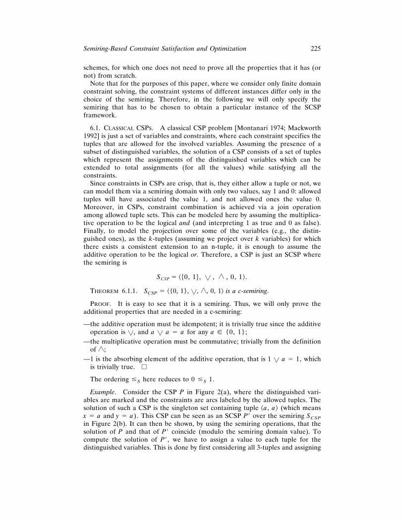
Example. Consider the CSP P in Figure 2(a), where the distinguished vari-ables are marked and the constraints are arcs labeled by the allowed tuples. Thesolution of such a CSP is the singleton set containing tuple â, a& (which meansx 5 a and y 5 a). This CSP can be seen as an SCSP P9 over the semiring SCSP

in Figure 2(b). It can then be shown, by using the semiring operations, that thesolution of P and that of P9 coincide (modulo the semiring domain value). Tocompute the solution of P9, we have to assign a value to each tuple for thedistinguished variables. This is done by first considering all 3-tuples and assigning


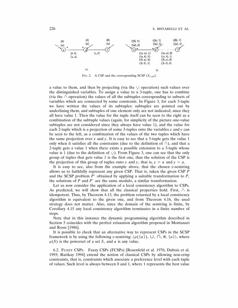
a value to them, and then by projecting (via the ~ operation) such values overthe distinguished variables. To assign a value to a 3-tuple, one has to combine(via the ` operation) the values of all the subtuples corresponding to subsets ofvariables which are connected by some constraint. In Figure 3, for each 3-tuplewe have written the values of its subtuples: subtuples are pointed out byunderlining them, and subtuples of one element only are not indicated, since theyall have value 1. Then the value for the tuple itself can be seen to the right as acombination of the subtuple values (again, for simplicity of the picture one-valuesubtuples are not considered since they always have value 1), and the value foreach 2-tuple which is a projection of some 3-tuples onto the variables x and y canbe seen to the left, as a combination of the values of the two tuples which havethe same projection over x and y. It is easy to see that a 3-tuple gets the value 1only when it satisfies all the constraints (due to the definition of `), and that a2-tuple gets a value 1 when there exists a possible extension to a 3-tuple whosevalue is 1 (due to the definition of ~). From Figure 3, one can see that the onlygroup of tuples that gets value 1 is the first one, thus the solution of the CSP isthe projection of this group of tuples onto x and y, that is, x 5 a and y 5 a.

It is easy to see, also from the example above, that the chosen c-semiringallows us to faithfully represent any given CSP. That is, taken the given CSP Pand the SCSP problem P9 obtained by applying a suitable transformation to P,the solutions of P and P9 are the same modulo, a similar transformation.

Let us now consider the application of a local consistency algorithm to CSPs.As predicted, we will show that all the classical properties hold. First, ` isidempotent. Thus, by Theorem 4.13, the problem returned by a local consistencyalgorithm is equivalent to the given one, and from Theorem 4.16, the usedstrategy does not matter. Also, since the domain of the semiring is finite, byCorollary 4.15 any local consistency algorithm terminates in a finite number ofsteps.

Note that in this instance the dynamic programming algorithm described inSection 5 coincides with the perfect relaxation algorithm proposed in Montanariand Rossi [1986].

It is possible to check that an alternative way to represent CSPs in the SCSPframework is by using the following c-semiring: ^`({a}), ø , ù , À, {a}&, where`(S) is the powerset of a set S, and a is any value.

6.2. FUZZY CSPS. Fuzzy CSPs (FCSPs) [Rosenfeld et al. 1976; Dubois et al.1993; Ruttkay 1994] extend the notion of classical CSPs by allowing non-crispconstraints, that is, constraints which associate a preference level with each tupleof values. Such level is always between 0 and 1, where 1 represents the best value

FIG. 2. A CSP and the corresponding SCSP (SCSP).


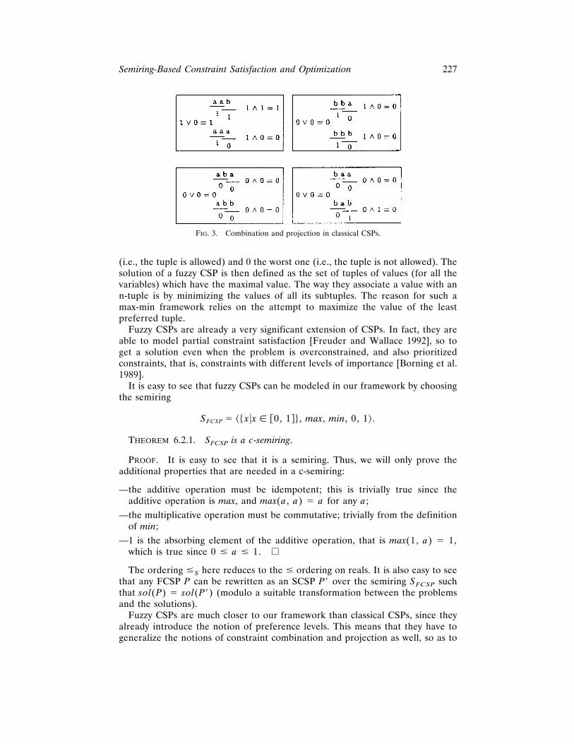
(i.e., the tuple is allowed) and 0 the worst one (i.e., the tuple is not allowed). Thesolution of a fuzzy CSP is then defined as the set of tuples of values (for all thevariables) which have the maximal value. The way they associate a value with ann-tuple is by minimizing the values of all its subtuples. The reason for such amax-min framework relies on the attempt to maximize the value of the leastpreferred tuple.

Fuzzy CSPs are already a very significant extension of CSPs. In fact, they areable to model partial constraint satisfaction [Freuder and Wallace 1992], so toget a solution even when the problem is overconstrained, and also prioritizedconstraints, that is, constraints with different levels of importance [Borning et al.1989].

It is easy to see that fuzzy CSPs can be modeled in our framework by choosingthe semiring

SFCSP 5 ^$ x ux [ @0, 1#% , max, min, 0, 1& .

THEOREM 6.2.1. SFCSP is a c-semiring.

PROOF. It is easy to see that it is a semiring. Thus, we will only prove theadditional properties that are needed in a c-semiring:

—the additive operation must be idempotent; this is trivially true since theadditive operation is max, and max(a, a) 5 a for any a;

—the multiplicative operation must be commutative; trivially from the definitionof min;

—1 is the absorbing element of the additive operation, that is max(1, a) 5 1,which is true since 0 # a # 1. e

The ordering #S here reduces to the # ordering on reals. It is also easy to seethat any FCSP P can be rewritten as an SCSP P9 over the semiring SFCSP suchthat sol(P) 5 sol(P9) (modulo a suitable transformation between the problemsand the solutions).

Fuzzy CSPs are much closer to our framework than classical CSPs, since theyalready introduce the notion of preference levels. This means that they have togeneralize the notions of constraint combination and projection as well, so as to

FIG. 3. Combination and projection in classical CSPs.


get the appropriate definition of solution. However, we are obviously much moregeneral in that we do not make any assumption on the semiring operations.

Let us now consider the properties that hold in the FCSP framework. Themultiplicative operation (i.e., min) is idempotent. Thus, local consistency algo-rithms on FCSPs do not change the solution of the given problem (by Theorem4.13), and do not care about the strategy (by Theorem 4.16). Moreover, min isAD-closed for any finite subset AD of [0, 1]. Thus, by Theorem 4.14, any localconsistency algorithm on FCSPs terminates.

Thus, FCSPs, although providing a significant extension to classical CSPs, canexploit the same kind of algorithms. Their complexity will of course be differentdue to the presence of more than two levels of preference. However, it can beproved that if the actually used levels of preference are p, then the complexity ofa local consistency algorithm is just O( p) times greater than that of thecorresponding algorithm over CSPs (as discussed also above and in Dubois et al.[1993].

An implementation of arc-consistency, suitably adapted to be used over fuzzyCSPs, is given in Schiex [1992]. However, no formal properties of its behavior areproved there. Thus, our result can be seen as a formal justification of Schiex[1992].

6.3. PROBABILISTIC CSPS. Probabilistic CSPs (Prob-CSPs) [Fargier and Lang1993] have been introduced to model those situations where each constraint chas a certain probability p(c), independent from the probability of the otherconstraints, to be part of the given real problem.10 This allows one to reason alsoabout problems that are only partially known. The probability levels on con-straints gives then, to each instantiation of all the variables, a probability that it isa solution of the real problem. This is done by first associating with each subsetof constraints the probability that it is in the real problem (by multiplying theprobabilities of the involved constraints), and then by summing up all theprobabilities of the subsets of constraints where the considered instantiation is asolution. Alternatively, the probability associated with an n-tuple t can also beseen as the probability that all constraints that t violates are indeed in the realproblem. This is just the product of all 1 2 p(c) for all c violated by t. Finally,the aim is to get those instantiations with the maximum probability.

The relationship between Prob-CSPs and SCSPs is complicated by the fact thatProb-CSPs contain crisp constraints with probability levels, while SCSPs containnoncrisp constraints. That is, we associate values with tuples, and not toconstraints. However, it is still possible to model Prob-CSPs, by using a transfor-mation which is similar to that proposed in Dubois et al. [1993] to modelprioritized constraints via soft constraints in the FCSP framework. More pre-cisely, we assign probabilities to tuples instead of constraints. Consider anyconstraint c with probability p(c), and let t be any tuple of values for thevariables involved in c. Then p(t) 5 1 if t is allowed by c, otherwise p(t) 5 1 2p(c). The reasons for such a choice are as follows: if a tuple is allowed by c andc is in the real problem, then t is allowed in the real problem; this happens withprobability p(c); if instead c is not in the real problem, then t is still allowed in

10 Actually, the probability is not of the constraint, but of the situation which corresponds to theconstraint: saying that c has probability p means that the situation corresponding to c has probabilityp of occurring in the real-life problem.


the real problem, and this happens with probability 1 2 p(c). Thus, t is allowedin the real problem with probability p(c) 1 1 2 p(c) 5 1. Consider instead atuple t which is not allowed by c. Then it will be allowed in the real problem onlyif c is not present; this happens with probability 1 2 p(c).

To give the appropriate value to an n-tuple t, given the values of all thesmaller k-tuples, with k # n and which are subtuples of t (one for eachconstraint), we just perform the product of the values of such subtuples. By theway values have been assigned to tuples in constraints, this coincides with theproduct of all 1 2 p(c) for all c violated by t. In fact, if a subtuple violates c,then by construction its value is 1 2 p(c); if instead a subtuple satisfies c, thenits value is 1. Since 1 is the unit element of 3, we have that 1 3 a 5 a for eacha. Thus, we get )(1 2 p(c)) for all c that t violates.

As a result, the semiring corresponding to the Prob-CSP framework is

Sprob 5 ^$ x ux [ @0, 1#% , max, 3, 0, 1& .

THEOREM 6.3.1. Sprob is a c-semiring.

PROOF. It is a semiring. To be also a c-semiring, we need the following:

—the additive operation must be idempotent; this is trivially true since theadditive operation is max, and max(a, a) 5 a for any a;

—the multiplicative operation must be commutative; trivially from the definitionof 3;

—1 is the absorbing element of the additive operation, that is max(1, a) 5 1,which is true since 0 # a # 1. e

The associated ordering #S here reduces to # over reals.It is easy to see that any Prob-CSP P can be rewritten as an SCSP (Sprob) P9

such that sol(P) 5 sol(P9) (modulo a suitable transformation between theproblems and the solutions). Note that the fact that P9 is a-consistent means thatin P there exists an n-tuple which has probability a to be a solution of the realproblem.

The multiplicative operation of Sprob (i.e., 3) is not idempotent. Thus, theresult of Theorem 4.13 cannot be applied to Prob-CSPs. That is, by applying alocal consistency algorithm one is not guaranteed to obtain an equivalentproblem. Theorem 4.16 cannot be applied as well. Thus, the strategy used by alocal consistency algorithm may matter. Also, 3 is not closed on any finitesuperset of any subset of [0, 1]. Thus the result of Theorem 4.14 cannot beapplied to Prob-CSPs. That is, we cannot be sure that a local consistencyalgorithm terminates.

As a result of these observations, local consistency algorithms may make nosense in the Prob-CSP framework. Thus, we are not sure that their applicationhas the desired properties (termination, equivalence, and order-independence).However, the fact that we are dealing with a c-semiring implies that, at least, wecan apply Theorem 4.3: if a Prob-CSP problem has a tuple with probability a tobe a solution of the real problem, then any subproblem has a tuple withprobability at least a to be a solution of a subproblem of the real problem. Thiscan be fruitfully used when searching for the best solution. In fact, if one employsa branch-and-bound search algorithm, and in one branch we find a partial


instantiation with probability smaller than a, then we can be sure that such abranch will never bring to a global instantiation with probability a. Thus, if aglobal instantiation with such a probability has already been found, we can cutthis branch. Similar (and possibly better) versions of branch-and-bound fornon-standard CSPs may be found in Freuder and Wallace [1992] and Schiex et al.[1995].

6.4. WEIGHTED CSPS. Whereas fuzzy CSPs associate a level of preferencewith each tuple in each constraint, in weighted CSPs (WCSPs) tuples come withan associated cost. This allows one to model optimization problems where the goal isto minimize the total cost (time, space, number of resources, . . .) of the proposedsolution. Therefore, in WCSPs the cost function is defined by summing up the costsof all constraints (intended as the cost of the chosen tuple for each constraint). Thus,the goal is to find the n-tuples (where n is the number of all the variables) whichminimize the total sum of the costs of their subtuples (one for each constraint).

Another way to understand the difference between WCSPs and FCSPs is thatFCSPs have an egalitarianistic approach to optimization problems (i.e., they aimat maximizing the overall level of consistency while balancing the levels of allconstraints), while WCSPs have an utilitarianistic approach (i.e., they aim atgetting the minimum cost globally, even though some constraints may beneglected and thus present a big cost) [Moulin 1988]. We believe that bothapproaches present advantages and drawbacks, and thus each of them may bepreferred to the other one, depending on the real-life situation to be modeled.

According to the informal description of WCSPs given above, the associatedsemiring is

SWCSP 5 ^51U$ 1 `% , min, 1, 1`, 0& .

THEOREM 6.4.1. SWCSP is a c-semiring.

PROOF. It is easy to see that it is a semiring. To be a c-semiring, we need:

—the additive operation must be idempotent; this is trivially true since theadditive operation is min, and min(a, a) 5 a for any a;

—the multiplicative operation must be commutative; trivially from the definitionof 1;

—0 is the absorbing element of the additive operation, that is min(0, a) 5 0,which is true since a $ 0. e

The associated ordering #S reduces here to $ over the reals. This means thata value is preferred to another one if it is smaller.

The multiplicative operation of SWCSP (i.e., 1) is not idempotent. Thus, theresults of Section 4 on local consistency algorithms cannot be applies to WCSPs.However, as in Prob-CSPs, the fact that we are dealing with a c-semiring impliesthat, at least, we can apply Theorem 4.3: if a WCSP problem has a best solutionwith cost a, then the best solution of any subproblem has a cost smaller than a.This can be fruitfully used when searching for the best solution in a branch-and-bound search algorithm.

Note that the same properties hold also for the semirings ^41U{1`}, min, 1,1`, 0& and ^]1U{1`}, min, 1, 1`, 0& (which can be proved to be c-semirings).


6.5. EGALITARIANISM AND UTILITARIANISM. As noted above, the FCSP andthe WCSP systems can be seen as two different approaches to give a meaning tothe notion of optimization. The two models correspond in fact to two definitionsof social welfare in utility theory [Moulin 1988]: egalitarianism, which maximizesthe minimal individual utility, and utilitarianism, which maximizes the sum of theindividual utilities. FCSPs are based on the egalitarian approach, while WCSPsare based on utilitarianism.

In this section, we will show how our framework allows also for the combina-tion of these two approaches. In fact, we will construct an instance of the SCSPframework, where the two approaches coexist, and allow us to discriminateamong solutions which otherwise would result indistinguishable. More precisely,we can first compute the solutions according to egalitarianism (i.e., using amax-min computation as in FCSPs), and then discriminate more among them viautilitarianism (i.e., using a max-sum computation as in WCSPs).

The resulting semiring is the following:

Sue 5 ^$^l, k& ul, k [ @0, 1#% , max, min, ^0, 0& , ^1, 1&&

where max and min are defined as follows:

—^l1, k1&max^l2, k2& 5 H^l1, max~k1, k2!&

^l1, k1&

if l1 5 l2

if l1 . l2

—^l1, k1&min^l2, k2& 5 H^l1, k1 1 k2&

^l2, k2&

if l1 5 l2

if l1 . l2

That is, the domain of the semiring contains pairs of values: the first element isused to reason via the max-min approach, while the second one is used to furtherdiscriminate via the max-sum approach. The operation min (which is themultiplicative operation of the semiring, and thus is used to perform theconstraint combination) takes two elements of the semiring, say a 5 â1, a2& andb 5 ^b1, b2&) and returns the one with the smallest first element if a1 Þ b1;otherwise, it returns the pair that has the sum of the second elements as itssecond element (i.e., â1, a2 1 b2&). The operation max performs a max on thefirst elements if they are different (thus, returning the pair with the maximumfirst element); otherwise (if a1 5 b1), it performs a max on the second elements(thus, returning a pair which has such a max as second element, that is, â1,max(a2, b2)&). More abstractly, we can say that, if the first elements of the pairsdiffer, then the max-min operations behave like a normal max-min; otherwise,they behave like max-sum. This can be interpreted as the fact that, if the firstelements coincide, it means that the max-min criterion cannot discriminateenough, and thus the max-sum criterion is used.

One can show that Sue is a c-semiring. However, since it uses a combination of theoperations of the semirings SFCSP and SWCSP, and since the multiplicative operationof SWCSP is not idempotent, also the multiplicative operation of Sue, that is, min, isnot idempotent. This means that we cannot guarantee that local consistencyalgorithms can be used meaningfully in this instance of the framework.

Note that also the opposite choice (i.e., first perform a max-sum and then amax-min) can be made, by using a similar c-semiring. However, due to the samereasoning as above, again the multiplicative operation would not be idempotent,


thus we cannot be sure that the local consistency techniques possess theproperties of Section 4.

6.6. SET-BASED CSPS. An interesting class of instances of the SCSP frame-work which are based on set operations like union and intersection is the onewhich uses the c-semiring

Sset 5 ^`~ A! , ø, ù, À, A& ,

where A is any set. It is easy to see that Sset is a c-semiring. Also, in this case theorder #Sset

reduces to set inclusion (in fact, a # b iff a ø b 5 b), and thereforeit is partial in general. Furthermore, 3 is ù in this case, and thus it isidempotent. Therefore, the local consistency algorithms possess all the propertiesstated in Section 4 and therefore can be applied. We recall that when a localconsistency algorithm is applied to an SCSP with a partially ordered semiring, itsapplication changes the constraints in a way that the new constraints are smallerthan the old ones in the ordering v.

A useful application of such SCSPs based on a set is when the variables of theproblem represent processes, the finite domain D is the set of possible states ofsuch processes, and A is the set of all time intervals over reals. In this case, avalue t associated to a pair of values ^d1, d2& for variables x and y can beinterpreted as the set of all time intervals in which process x can be in state d1and process y in state d2. Therefore, a solution of any SCSP based on thec-semiring Sset consists of a tuple of process states, together with (the set of) thetime intervals in which such system configuration can occur. This description of asystem can be helpful, for example, to discover if there are time intervals inwhich a deadlock is possible.

7. N-Dimensional c-Semirings

Choosing an instance of the SCSP framework means specifying a particularc-semiring. This, as discussed above, induces a partial order which can beinterpreted as a (partial) guideline for choosing the “best” among differentsolutions. In many real-life situations, however, one guideline is not enough,since, for example, it could be necessary to reason with more than one objectivein mind, and thus choose solutions which achieve a good compromise withrespect to all such goals.

Consider for example a network of computers, where one would like to bothminimize the total computing time (thus the cost) and also to maximize the workof the least used computers. Then, in our framework, we would need to considertwo c-semirings, one for cost minimization (see Section 6.4 on weighted CSPs),and another one for work maximization (see Section 6.2 on fuzzy CSPs). Thenone could work first with one of these c-semirings and then with the other one,trying to combine the solutions which are the best for each of them. However, amuch simpler approach consists of combining the two c-semirings and only thenwork with the resulting structure. The nice property is that such a structure is ac-semiring itself; thus, all the techniques and properties of the SCSP frameworkcan be used for such a structure as well.


More precisely, the way to combine several c-semirings and getting anotherc-semiring just consists of vectorizing the domains and operations of the com-bined c-semirings.

Definition 7.1 (composition of c-semirings). Given n c-semirings Si 5 ^ Ai,1 i, 3 i, 0i, 1i&, for i 5 1, . . . , n, let us define the structure Comp(S1, . . . , Sn)5 ^^ A1, . . . , An&, 1, 3, ^01, . . . , 0n&, ^11

. . . 1n&&. Given â1, . . . , an& and^b1, . . . , bn& such that ai, bi [ Ai for i 5 1, . . . , n, â1, . . . , an& 1 ^b1, . . . ,bn& 5 â1 11 b1, . . . , an 1n bn&, and â1, . . . , an& 3 ^b1, . . . , bn& 5 â1 31b1, . . . , an 3n bn&.

We will now prove that by composing c-semirings we get another c-semiring.This means that we all the properties of the framework defined in the previoussections hold.

THEOREM 7.2 (A C-SEMIRING COMPOSITION IS A C-SEMIRING). Given n c-semirings Si 5 ^ Ai, 1i, 3i, 0i, 1i&, for i 5 1, . . . , n, the structure Comp(S1, . . . , Sn)is a c-semiring.

PROOF. It is easy to see that all the properties required for being a c-semiringhold for Comp(S1, . . . , Sn), since they directly follow from the correspondingproperties of the component semirings Si. e

According to the definition of the ordering #S (in Section 2), such an orderingfor S 5 Comp(S1, . . . , Sn) is as follows. Given â1, . . . , an& and ^b1, . . . , bn&such that ai, bi [ Ai for i 5 1, . . . , n, we have â1, . . . , an& #S ^b1, . . . , bn&if and only if â1 11 b1, . . . , an 1n bn& 5 ^b1, . . . , bn&. Since the tupleelements are completely independent, #S is in general a partial order, even ifeach of the #Si

is a total order. This means (see Section 3) that the abstractsolution of a problem over such a semiring in general contains an incomparableset of tuples, none of which has blevel(P) as its associated value. Therefore, ifone wants to reduce the number of “best” tuples (or to get just one), one has tospecify some priorities among the orderings of the component c-semirings.

Notice that, although the c-semiring discussed in Section 6.4 may seem acomposition of two c-semirings, as defined in Definition 7.1, this is not so, sincethe behavior of each of the two operations on one of the two elements of eachpair (we recall that that semiring is a set of pairs) is not independent from thebehavior of the same operation on the other element of the pair. Thus it is notpossible to define two independent operations (i.e., 11 and 12, or 31 and 32), asneeded by Definition 7.1. For example, operation max returns the maximum ofthe second elements of two pairs only when the first elements of the pairs areequal.

8. Conclusion and Future Work

We have proposed a general framework for constraint solving where each tuple isallowed by a constraint with a certain level of confidence (or degree, or cost,etc.). This allows for a more realistic modelization of real-life problems, butrequires a new constraint solving engine which has to take such levels intoaccount. To do this, we used the notion of semiring, which provides both thelevels and the new constraint combination operations. We also considered the


issue of local consistency in such an extended framework, and we providedsufficient conditions which assure the local consistency algorithms to work in theextended framework. Then, we considered dynamic programming-like algo-rithms, and we proved that these algorithm can always be applied to SCSPs, andhave a linear time complexity when the given SCSPs can be provided with aparsing tree of bounded size. Finally, we provided several instances of SCSPswhich show the generality and also the expressive power of the framework.

As it may be difficult to assign each tuple in each constraint with a value fromthe semiring, but it may be instead easy to rate some solutions, we are currentlyinvestigating the possibility of learning values for all the tuples from someexamples of solution ratings, via the use of classical gradient-descent learningalgorithms [Rossi and Sperduti 1996]. This would greatly enhance the practicalusefulness of SCSPs.

As classical constraint solving has been embedded into Constraint LogicProgramming (CLP) [Jaffar and Lassez 1987] systems, it is reasonable to thinkthat also our more general notion of constraint solving can be handled within alogic language, thus giving rise to new instances of the CLP scheme. This wouldnot only give new meanings to constraint solving in CLP, but it would also allowone to treat in a uniform way optimization problem solving within CLP, withoutthe need to resort to ad hoc methods as in Van Hentenryck [1989]. In fact, itwould be possible to generalize the semantics of CLP programs to consider thechosen semiring and thus solve problems according to the semiring operations.This could be done by associating with each ground atom an element of thesemiring and by using the two semiring operations to combine goals. These issueshave been studied already for the instance of WCSPs in Bistarelli [1994]. Weplan to do it in the general case as well.

ACKNOWLEDGMENTS. We would like to thank the Esprit BRA project ACCLAIM(n. 7195) for partially supporting the initial stages of this research, Thomas Schiexfor many enlightening discussions on this subject, and the anonymous referees for allthe useful comments on previous versions of this paper.

REFERENCES

BELLMAN, R. E. 1957. Dynamic Programming. Princeton University Press, Princeton, N.J.BELLMAN, R. E., AND DREYFUS, S. E. 1962. Applied Dynamic Programming. Princeton University

Press, Princeton, N.J.BERTELE, U., AND BRIOSCHI, F. 1972. Nonserial Dynamic Programming. Academic Press, Orlando, Fla.BISTARELLI, S. 1994. Programmazione con vincoli pesati e ottimizzazione (in Italian). Tech. Rep.

Dipartmento di Informatica, Universita di Pisa, Pisa, Italy.BISTARELLI, S., FARGIER, H., MONTANARI, U., ROSSI, F., SCHIEX, T., AND VERFAILLE, G. 1996.

Semiring-based CSPs and valued CSPs: Basic properties and comparison. In Over-ConstrainedSystems, M. Jampel, ed. Lecture Notes in Computer Science, Vol. 1106. Springer-Verlag, NewYork.

BISTARELLI, S., MONTANARI, U., AND ROSSI, F. 1995. Constraint solving over semirings. InProceedings of the International Joint Conference on Artificial Intelligence (IJCAI95). Morgan-Kaufmann, San Mateo, Calif., pp. 624 – 630.

BORNING, A., MAHER, M., MARTINDALE, A., AND WILSON, M. 1989. Constraint hierarchies andlogic programming. In Proceeding of the 6th International Conference on Logic Programming. MITPress, Cambridge, Mass., pp. 149 –164.

COUSOT, P. 1977. Asynchronous iterative methods for solving a fixed point system of monotoneequations in a complete lattice. Tech. Rep. R.R.88. Institut National Polytechnique de Grenoble,Grenoble, Switzerland.


DAVEY, B. A., AND PRIESTLY, H. A. 1990. Introductions to Lattices and Order. CambridgeUniversity Press, Cambridge, England. pp. 37– 42.

DECHTER R., AND DECHTER, A. 1988. Brief maintenance in dynamic constraint networks. InProceedings of the AAAI88. Morgan-Kaufmann, San Mateo, Calif., pp. 37– 42.

DECHTER, R., DECHTER, A., AND PEARL, J. 1990. Optimization in constraint networks. In InfluenceDiagrams, Belief Nets and Decision Analysis, R. M. Oliver and J. Q. Smith, eds. Wiley, New York, pp.411–425.

DECHTER, R., AND PEARL, J. 1988a. Network-based heuristics for constraint-satisfaction problems.In Search in Artificial Intelligence, Kanal and Kumar, eds. Springer-Verlag, New York, pp. 370 – 425.

DECHTER, R., AND PEARL, J. 1988b. Tree-clustering schemes for constraint processing. In Proceed-ings of the AAAI88. Morgan-Kaufmann, San Mateo, Calif., pp. 150 –154.

DUBOIS, D., FARGIER, H., AND PRADE, H. 1993. The calculus of fuzzy restrictions as a basis forflexible constraint satisfaction. In Proceedings of the IEEE International Conference on FuzzySystems. IEEE, New York, pp. 1131–1136.

FARGIER, H., AND LANG, J. 1993. Uncertainty in constraint satisfaction problems: A probabilisticapproach. In Proceedings of the European Conference on Symbolic and Qualitative Approaches toReasoning and Uncertainty (ESQUARU). Lecture Notes in Computer Science, vol. 747. Springer-Verlag, New York, pp. 97–104.

FREUDER, E. C. 1978. Synthesizing constraint expressions. Commun. ACM 21, 11 (Nov.), 958 –965.FREUDER, E. C. 1988. Backtrack-free and backtrack-bounded search. In Search in Artificial

Intelligence, Kanal and Kumar, eds. Springer-Verlag, New York, pp. 343–369.FREUDER, E. C., AND WALLACE, R. J. 1992. Partial constraint satisfaction. AI J. 58, 21–70.GIACOBAZZI, R., DEBRAY, S. K., AND LEVI, G. 1992. A generalized semantics for constraint logic

programs. In Proceedings of Fifth Generation Computer Systems (FGCS92). ICOT, Tokyo, Japan,pp. 581–591.

GNESI, S., MONTANARI, U., AND MARTELLI, A. 1981. Dynamic programming as graph searching:An algebraic approach. J. ACM 28, 4 (Oct.), 737–751.

GYSSENS, M., JEAVONS, P. G., AND COHEN, D. A. 1994. Decomposing constraint satisfactionproblems using database techniques. Artif. Int. 66, 1, 57– 89.

JAFFAR, J., AND LASSEZ, J. L. 1987. Constraint logic programming. In Proceedings of Principles ofProgramming Languages (Munich, West Germany, Jan. 21–23). ACM, New York, pp. 111–119.

KUMAR, V. 1992. Algorithms for constraint satisfaction problems: A survey. AI Mag. 13, 1, 32– 44.MACKWORTH, A. K. 1977. Consistency in networks of relations. Artif. Int. 8, 1, 99 –118.MACKWORTH, A. K. 1992. Constraint satisfaction. In Encyclopedia of AI, 2nd ed., vol. 1, S. C.

Shapiro, ed. Wiley, New York, pp. 285–293.MACKWORTH, A. K., AND FREUDER, E. C. 1984. The complexity of some polynomial network

consistency algorithms for constraint satisfaction problems. Artif. Int. 25, 65–74.MARTELLI, A., AND MONTANARI, U. 1972. Nonserial dynamic programming: On the optimal

strategy of variable elimination for the rectangular lattice. J. Math. Anal. Appl. 40, 226 –242.MONTANARI, U. 1974. Networks of constraints: Fundamental properties and application to picture

processing. Inf. Sci. 7, 95–132.MONTANARI, U., AND ROSSI, F. 1986. An efficient algorithm for the solution of hierarchical

networks of constraints. In Proceedings of the International Workshop on Graph Grammars and TheirApplication to Computer Science. Lecture Notes in Computer Science, vol. 291. Springer-Verlag,New York, pp. 440 – 457.

MONTANARI, U., AND ROSSI, F. 1991. Constraint relaxation may be perfect. AI J. 48, 143–170.MOULIN, H. 1988. Axioms for Cooperative Decision Making. Cambridge University Press, Cam-

bridge, Mass.ROSENFELD, A., HUMMEL, R. A., AND ZUCKER, S. W. 1976. Scene labelling by relaxation opera-

tions. IEEE Trans. Syst., Man, Cyber 6, 6, 420 – 433.RUTTKAY, ZS. 1994. Fuzzy constraint satisfaction. In Proceedings of the IEEE 3rd International

Conference on Fuzzy Systems. IEEE, New York, pp. 1263–1268.ROSSI, F., AND SPERDUTI, A. 1996. Learning solution preferences in constraint problems. In

Proceedings of the International Workshop on Non-Standard Constraint Processing at ECAI96. Taylorand Francis publishers. (A longer version will appear in J. Exp. Theor. Artif. Int.)

SCHIEX, T. 1992. Possibilistic constraint satisfaction problems or “how to handle soft constraints?”In Proceedings of the 8th Conference of Uncertainty in Artificial Intelligence. pp. 269 –275.


SCHIEX, T., FARGIER, H., AND VERFAILLE, G. 1995. Valued constraint satisfaction problems: Hardand easy problems. In Proceedings of the International Joint Conference on Artificial Intelligence(IJCAI95). Morgan-Kaufmann, San Mateo, Calif., pp. 631– 637.

SHENOY, P. 1991. Valuation-based systems for discrete optimization. In Uncertainty in ArtificialIntelligence, L. N. Kanal, P. P. Bonissone, M. Henrion, and J. F. Lemayer, eds. Elsevier Science,Amsterdam, The Netherlands.

SHENOY, P. 1994. Valuation-based systems: A framework for managing uncertainty in expertsystems. In Fuzzy Logic for the Management of Uncertainty, L. Zadeh and J. Kacprzyk, eds. Wiley,New York, pp. 83–104.

VAN HENTENRYCK, P. 1989. Constraint Satisfaction in Logic Programming. MIT Press, Cambridge, Mass.ZADEH, L. A. 1965. Fuzzy sets. Inf. Control 8, 338 –353.

RECEIVED SEPTEMBER 1995; REVISED FEBRUARY 1997; ACCEPTED DECEMBER 1996

Journal of the ACM, Vol. 44, No. 2, March 1997.


Documents

Semiring-based constraint satisfaction and optimization