Embed Size (px)
Citation preview
Sensitivity analysis methodologies for analysing emergence using
agent-based modelsGuus ten Broeke
Sen
sitivity analysis m
ethod
ologies for an
alysing
emerg
ence u
sing
agen
t-based
mod
elsG
uus ten Broeke

Propositions
1. Sensitivity analysis is a necessity for drawing general conclusions from
simulation models.
(this thesis)
2. Global sensitivity indices yield little insight into emergent behaviour of
agent-based models.
(this thesis)
3. Scientific publication of simulation models without complete
documentation leads to a lack of replicability, and is therefore
detrimental to scientific progress.
4. Metaphors about complex systems are usually more misleading than
helpful.
5. To promote creative thinking, failure should be more appreciated than
is presently the case in education and science.
6. The KISS (keep it simple, stupid) design principle (Axelrod, R. M. The
complexity of cooperation: Agent-based models of competition and
collaboration. Princeton University Press, 1997) applies as much to life
as to modelling.
7. To fulfil a job optimally, it is best to spend your free time doing other
things.
Propositions belonging to the thesis, entitled
‘Sensitivity analysis methodologies for analysing emergence using agent-based
models’
Guus ten Broeke
Wageningen, October 25 2017.
Sensitivity analysis methodologiesfor analysing emergence using
agent-based models
Guus ten Broeke

Thesis committee:
Promotor:Prof. Dr. J.MolenaarProfessor of Applied MathematicsWageningen University & Research
Co-promotors:Dr. G.A.K. van VoornResearch Scientist, Mathematical and Statistical Methods GroupWageningen University & Research
Dr. Ir. A. LigtenbergAssistent Professor, Laboratory of Geo-Information and Remote SensingWageningen University & Research
Other members:Prof. Dr. C. Kroeze, Wageningen University & ResearchProf. Dr. C.K. Hemelrijk, Rijksuniversiteit GroningenDr.Ir. G.J. Hofstede, Wageningen University & ResearchDr. B. Edmonds, Manchester Metropolitan University, UK
This research was conducted under the auspices of the C.T. de Wit Graduate School forProduction Ecology and Resource Conservation (PE&RC)
Sensitivity analysis methodologies foranalysing emergent phenomena using
agent-based models
Guus ten Broeke
Thesissubmitted in fulfilment of the requirements for the degree of doctor
at Wageningen Universityby the authority of the Rector Magnificus
Prof. Dr. A.P.J. Molin the presence of the
Thesis Committee appointed by the Academic Boardto be defended in public
on Wednesday 25 October 2017at 4 p.m. in the Aula

Guus ten BroekeSensitivity analysis methodologies for analysing emergence using agent-based models,212 pages.
PhD thesis Wageningen University, Wageningen, NL (2017)With references, with summaries in English and Dutch.
ISBN 978-94-6343-699-1DOI http://dx.doi.org/10.18174/423172
Contents
1 General Introduction 11.1 Complex adaptive systems . . . . . . . . . . . . . . . . . . . . . . . . . 21.2 CAS models . . . . . . . . . . . . . . . . . . . . . . . . . . . . . . . . . 31.3 Challenges . . . . . . . . . . . . . . . . . . . . . . . . . . . . . . . . . . 71.4 Sensitivity analysis . . . . . . . . . . . . . . . . . . . . . . . . . . . . . 101.5 Objectives . . . . . . . . . . . . . . . . . . . . . . . . . . . . . . . . . . 111.6 Approach . . . . . . . . . . . . . . . . . . . . . . . . . . . . . . . . . . 121.7 Thesis outline . . . . . . . . . . . . . . . . . . . . . . . . . . . . . . . . 12
2 Automated sensitivity analysis for ecological dynamical models 152.1 Introduction . . . . . . . . . . . . . . . . . . . . . . . . . . . . . . . . . 162.2 Local sensitivity analysis . . . . . . . . . . . . . . . . . . . . . . . . . . 182.3 Examples . . . . . . . . . . . . . . . . . . . . . . . . . . . . . . . . . . 202.4 Discussion . . . . . . . . . . . . . . . . . . . . . . . . . . . . . . . . . . 262.A Local sensitivity analysis . . . . . . . . . . . . . . . . . . . . . . . . . . 272.B Ricker model . . . . . . . . . . . . . . . . . . . . . . . . . . . . . . . . 302.C Rosenzweig-MacArthur model . . . . . . . . . . . . . . . . . . . . . . . 33
3 Detecting Tipping points with Sensitivity Analysis 433.1 Introduction . . . . . . . . . . . . . . . . . . . . . . . . . . . . . . . . . 443.2 Sensitivity analysis methodologies . . . . . . . . . . . . . . . . . . . . 473.3 Case description . . . . . . . . . . . . . . . . . . . . . . . . . . . . . . 523.4 Results of sensitivity analysis . . . . . . . . . . . . . . . . . . . . . . . 553.5 Discussion & Conclusions . . . . . . . . . . . . . . . . . . . . . . . . . 633.A Direct differential method . . . . . . . . . . . . . . . . . . . . . . . . . 653.B Local sensitivity analysis of the Bazykin-
Berezovskaya model . . . . . . . . . . . . . . . . . . . . . . . . . . . . 653.C Distribution of local sensitivity indices . . . . . . . . . . . . . . . . . . 663.D Variance decomposition in Sobol’ method . . . . . . . . . . . . . . . . 673.E Sobol’ indices in the steady state . . . . . . . . . . . . . . . . . . . . . 693.F Sampling method for the Sobol’ indices . . . . . . . . . . . . . . . . . 70
4 Which sensitivity analysis method should I use for my ABM? 754.1 Introduction . . . . . . . . . . . . . . . . . . . . . . . . . . . . . . . . . 764.2 Selected goals for performing sensitivity analysis . . . . . . . . . . . . 774.3 Selected methodologies for sensitivity analysis . . . . . . . . . . . . . . 78

vi CONTENTS
4.4 Model test case: agents harvesting a diffusing renewable resource . . . 814.5 Model results . . . . . . . . . . . . . . . . . . . . . . . . . . . . . . . . 844.6 Discussion . . . . . . . . . . . . . . . . . . . . . . . . . . . . . . . . . . 924.A Model description . . . . . . . . . . . . . . . . . . . . . . . . . . . . . . 964.B OFAT results . . . . . . . . . . . . . . . . . . . . . . . . . . . . . . . . 1044.C Consequences of the choice of sampling design . . . . . . . . . . . . . . 104
5 Resilience through adaptation 1115.1 Introduction . . . . . . . . . . . . . . . . . . . . . . . . . . . . . . . . . 1125.2 Materials and Methods . . . . . . . . . . . . . . . . . . . . . . . . . . . 1135.3 Results . . . . . . . . . . . . . . . . . . . . . . . . . . . . . . . . . . . . 1205.4 Conclusions & Discussion . . . . . . . . . . . . . . . . . . . . . . . . . 1285.A Stationarity and ergodicity tests . . . . . . . . . . . . . . . . . . . . . 1315.B Computation of the earth mover’s distance. . . . . . . . . . . . . . . . 1335.C Results of stationarity and ergodicity tests. . . . . . . . . . . . . . . . 1345.D Default parameter setting . . . . . . . . . . . . . . . . . . . . . . . . . 139
6 Cooperation can improve resilience 1416.1 Introduction . . . . . . . . . . . . . . . . . . . . . . . . . . . . . . . . . 1426.2 Model Description . . . . . . . . . . . . . . . . . . . . . . . . . . . . . 1446.3 Model analysis methodology . . . . . . . . . . . . . . . . . . . . . . . . 1466.4 Results . . . . . . . . . . . . . . . . . . . . . . . . . . . . . . . . . . . . 1516.5 Conclusions & Discussion . . . . . . . . . . . . . . . . . . . . . . . . . 1596.A Model Description . . . . . . . . . . . . . . . . . . . . . . . . . . . . . 1616.B One-factor-at-a-time results for growth rate r . . . . . . . . . . . . . . 1756.C Global sensitivity analysis . . . . . . . . . . . . . . . . . . . . . . . . . 175
7 General Discussion 1797.1 Aims of sensitivity analysis . . . . . . . . . . . . . . . . . . . . . . . . 1797.2 Evaluation of sensitivity analysis methodologies . . . . . . . . . . . . . 1807.3 Lessons from applying sensitivity analysis to ABMs . . . . . . . . . . 1837.4 Future work . . . . . . . . . . . . . . . . . . . . . . . . . . . . . . . . . 185
Bibliography 189
Summary 199
Summary 201

Chapter 1
General Introduction
2 General Introduction
1.1 Complex adaptive systemsHuman and natural systems usually show complex behaviour that cannot be un-derstood by studying in isolation the constituent components. Examples includeeconomic markets (Tesfatsion 2003), ecosystems (Levin 1998), supply networks (Nairet al. 2009), and land-use systems (Parker et al. 2003). All these systems are com-posed of a large number of components, which are influenced both by mutual inter-actions and by interactions with the environment. The components are autonomousin the sense that they have their own objectives, and make their own decisions inorder to achieve these objectives. The system-level behaviour emerges from interac-tions between these components. Ecosystems, for example, contain large numbersof autonomous and interacting organisms. These individual organisms are aimed atachieving individual-level goals, rather than system-level goals. At the system-level,these interactions form a balance that leads to more or less stable patterns over time,such as distributions of nutrient patterns and trace elements, or characteristic abun-dance distributions of species (Levin 2003). These patterns, which are importantfor sustaining life, emerge from mutual interactions between organisms, as well frominteractions with their physical and chemical environment. The system as a wholeappears to possess a great degree of coordination. Understanding this coordinationis not possible by studying only the characteristics of the individual organisms orspecies, but requires studying the interactions within the system.
The framework of complex adaptive systems (CAS) is eminently appropriate forstudying how complex behaviour at system level may emerge from interactions be-tween lower-level components. A central idea behind CAS is that the mechanismsunderlying this emergence share similarities across a wide range of systems. Thus,even though economies, ecosystems, and immune systems are entirely different sys-tems, lessons from studying one of these types of systems, may be generalised to theother types.
There exists no universally accepted definition of CAS, but some essential prop-erties are generally agreed upon (Railsback 2001, Holland 2002, Levin 2003).
• Autonomous agents. CAS are composed of autonomous units, or agents thatact according to their individual objectives. Depending on the system, theseagents may for example represent people, animals, or companies.
• Observation. Agents observe their environment, i.e., the state of their physicalsurroundings and the state of other agents.
• Observation-based actions. The observations of agents influence their decision-making process.
• Interactions. Agents have the capacity to make changes to their environment,and to influence other agents.
• Agent adaptation. As a result of interactions the characteristics of agent popula-tions may change over time, for example through a process of natural selection.
• Learning. Agents can change their decision rules based on previous experiences,for example through trial-and-error, or imitation of other agents. Learning dif-fers from adaptation, in that adaptation refers to changes in the distribution of
Chapter 1 3
characteristics across a population, whereas learning is based on the experienceof individual agents.
• Emergence. The system-level properties of CAS cannot be a priori predictedfrom the properties of the agents, but are emergent.
Essential is that CAS is a bottom-up approach, in which system-level propertiesemerge from lower-level components. Some examples of this emergence are discussedin the following paragraphs, and it will remain a central concept throughout thisthesis.
1.2 CAS models
Since the system-level behaviour of CAS emerges from lower-level interactions, it istypically difficult to analyse CAS using direct observations or experiments (Railsbackand Grimm 2011). Whereas in physics, interactions between individual particles canbe statistically aggregated to derive system-level properties, such an approach hasproven to be of little use in the social sciences due to the complexity and diversityof interactions and heterogeneity of agents (Lansing 2003). For example, interactionsin human societies are local, strongly non-linear, and dependent on individual differ-ences between agents. Furthermore, keeping track of all the individual agents andinteractions between agents in a system is typically not feasible in a practical situa-tion (Gilbert 2004). Thus, understanding of the emergence of patterns in society haslong remained out of reach.
Thanks to the development of computers, the field of social simulation has pro-vided us with a tool for gaining insight into CAS. Simulation models are simplifiedrepresentations of real-life systems in which interactions between agents can be mod-elled to investigate their effects at system level. The role of simulation models forstudying CAS is comparable to that of thought experiments in physics (Holland2002). They can be used to formalise assumptions about interactions between systemcomponents, and to systematically explore the consequences of these assumptions. Inthis way, simulation models allow us to perform ’experiments’ that cannot be per-formed in real-life systems. Such experiments are of great help to develop theories onsocial processes and to generate new hypotheses.
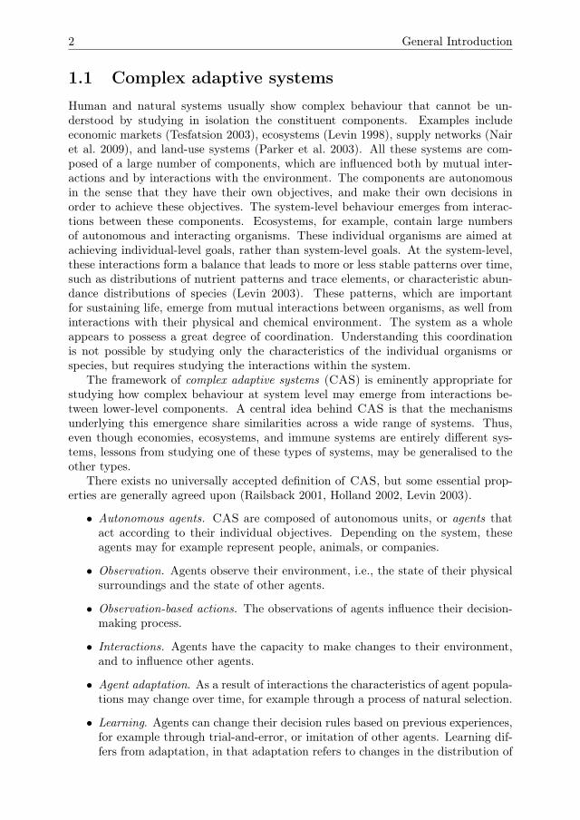
It should of course be tested whether the assumptions behind any simulation modelare appropriate, given the context of the study. Together with the conceptualisationand development of the simulation model, this testing is part of an iterative process.This process is commonly represented in terms of a modelling cycle (Fig 1.1). Basedon the real-life system, a conceptual model is developed. Crucial to this developmentis the research question that the model is intended to answer, as well as the formulatedhypotheses regarding this research question. The model should have the right level ofdetail to test these hypotheses (Grimm et al. 2005). A model is too simple if it does nottake into account mechanisms that are essential to test the formulated hypotheses. If,in contrast, the model contains many unessential details, it may become impossible toanalyse it in the context of these hypotheses. Once a conceptual model with the rightlevel of detail has been developed, it is represented in terms of computer code. Themodel is then analysed to see what can be learned from it about the real world. Of
4 General Introduction
Figure 1.1: Modelling cycle (simplified from Refsgaard and Henriksen (2004), van Voornet al. (2016)). Modelling often involves going back and forth between thesesteps, as denoted by the inner arrows. The cycle as a whole proceeds clockwise,as denoted by the arrows on the outer curve.
course, this cycle is a simplified representation of the modelling process. In practice,modelling often involves going back and forth between different steps, rather thangoing once through the cycle.
Various modelling methods have been used to describe CAS. In this thesis, we fo-cus on two types of models, namely ordinary differential equation (ODE) models andagent-based models (ABM). These modelling methods are discussed below, includingtheir strengths and weaknesses for modelling CAS.
1.2.1 Ordinary differential equation models
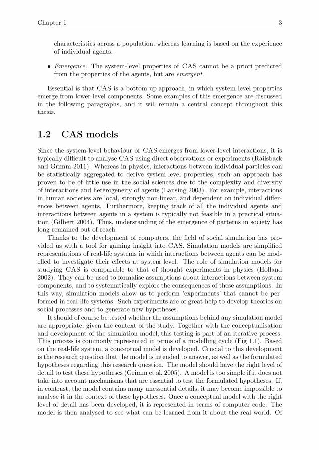
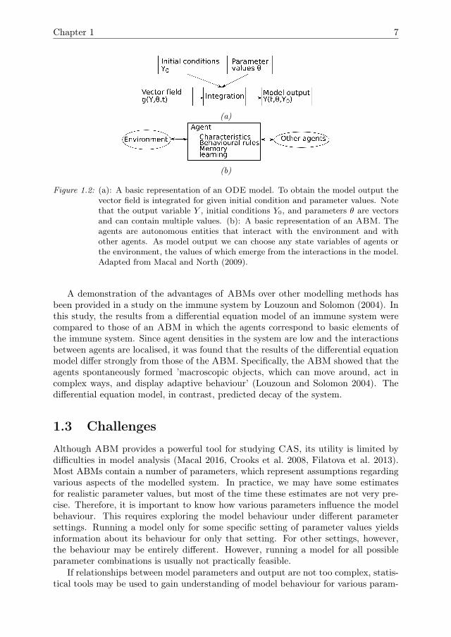
Differential equation models are used in a wide range of fields, such as physics, chem-istry, engineering, biology, and economics. Fig 1.2a shows a graphical representationof differential equation models. A differential equation relates a function to its ownderivative(s). In this thesis, only models with a single derivative with respect totime will be considered. Differential equations with a single independent variable(i.e. time) are referred to as ordinary differential equations (ODE)s. The vector fielddY (t, θ, Y0)/dt = g(Y (t, θ, Y0), θ) quantifies the change of the state variables Y withrespect to time, depending on the values of the parameters θ and initial conditionsY0. Usually, Y , Y0, and θ are vectors. Thus an ODE model may contain multiplestate variables and parameters. The vector field of one state variable may dependon the values of other state variables. Such dependencies can be used to describe in-teractions between state variables. The model output Y (t, θ, Y0) can be obtained byintegrating the vector field over time. For some simple ODE models this integrationcan be done analytically, which then yields an explicit solution for the values of thestate variables as function of time. For most models, no exact solution is available.Numerical methods may then be used to approximate the solution.
An example of an ODE model from ecology is the Lotka-Volterra model ofpredator-prey interaction. This example will be discussed here because ODE modelsof predator-prey interaction are extensively used in the second and third chapter ofthis thesis. The model reads as
dY1
dt= αY1 − βY1Y2 (1.1a)
Chapter 1 5
dY2
dt= βδY1Y2 − γY2 (1.1b)
with initial conditions
Y1(0) = Y1,0 (1.1c)Y2(0) = Y2,0. (1.1d)
Here Y1 is the prey density, Y2 the predator density, and t time. The population den-sities Y1 and Y2 are functions of time, the initial conditions, and the model parametersso Y1 = Y1(t, Y1,0, Y2,0, α, β, γ, δ), and likewise for Y2. The parameter α describes theintrinsic growth rate of the prey population, γ the predator mortality rate, β the pre-dation rate coefficient, and δ the efficiency of biomass conversion. All symbols usedin this chapter are listed in Table 1.1. Eqs (1.1a,1.1b) express the change in time ofboth populations as function of the population densities and model parameters. Fromthese equations the population densities can be obtained as function of time, givenvalues for the initial conditions Y1,0 and Y2,0.
Predator-prey ODE models like the Lotka-Volterra model are based on severalassumptions that are important to consider in the context of CAS. Note that inEq 1.1a the predator and prey populations, each of which consist of a large numberof individual animals, are described by a single variable representing the populationdensity. So, it is assumed that the population consists of identical individuals thatdo not adapt over time. Furthermore, the interactions between species are defined atthe population level. It is thus assumed that each individual has an equal effect oneach other individual (Huston et al. 1988). Although there are some possibilities forrepresenting more detailed interactions or individual differences, ODE models are notsuitable for representing local interactions between large numbers of heterogeneousagents. In many physical and social systems, however, it is important to considerlocality of interactions and heterogeneity of agents. For example, in social systemspeople are influenced mostly by specific people in their surroundings, rather thanbeing influenced equally by every member of the population. For systems in whichlocal interactions between heterogeneous agents are expected to be important, ODEmay not be the most suitable modelling method.
Even though ODE models may not be suitable for modelling local interactions andheterogeneous agents, such models are used extensively in the second of third chaptersof this thesis. The reason is that some ODE models share important characteristicswith CAS models, and the comparison with ODE models can yield valuable insightsthat are applicable to CAS models. One such property, central in chapters 3 and 4of this thesis, is that the model may display various long-term behaviours dependingon the initial conditions and parameter values. As an example, we again considerthe Lotka-Volterra model 1.1a. It can be shown that for positive initial populations(Y1,0 > 0 and Y2,0 > 0) the model converges to a long-term solution in which bothpopulations oscillate periodically. Alternative solutions are found when Y1,0 = 0 orY2,0 = 0. When Y2,0 = 0, the system contains no predators, and the prey popula-tion will continue to grow exponentially. When Y1,0 = 0, there is no prey, leadingto extinction of the predator population. This example might seem trivial due toits simplicity, but in general ODE models can display various types of long-termbehaviour and analysing this behaviour is usually no straightforward task. The tran-
6 General Introduction
sitions between these types of behaviour in parameter space are referred to as tippingpoints.
An advantage of ODE models is the availability of well-developed tools for modelanalysis. Methods of bifurcation analysis (Kuznetsov 2004) are available to detecttipping points. Tipping points may also be an important property for other typesof CAS models, as will be discussed in Section 1.3.1. But for these models bifur-cation analysis is not applicable. In this thesis, methods to detect tipping points inCAS models will be proposed. ODE models will be used to test these methods bycomparing their outcomes to those of existing bifurcation analysis methodologies.
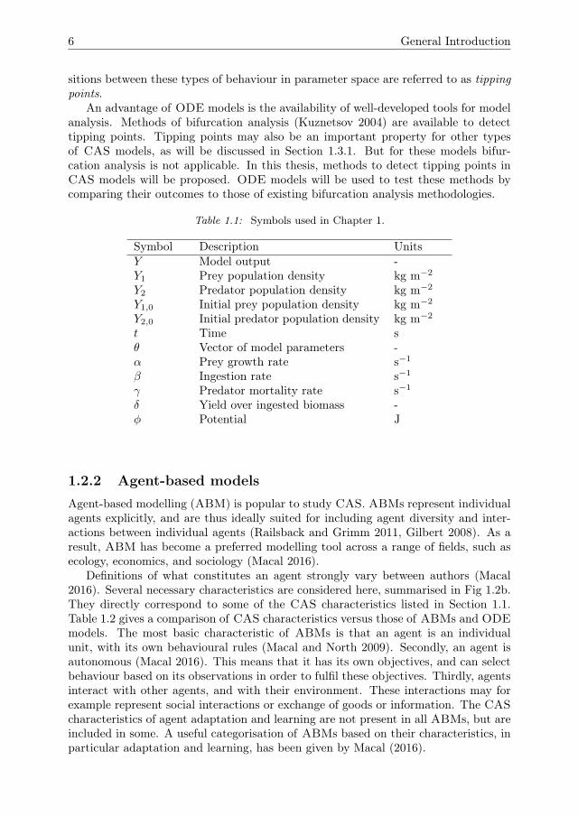
Table 1.1: Symbols used in Chapter 1.
Symbol Description UnitsY Model output -Y1 Prey population density kg m−2
Y2 Predator population density kg m−2
Y1,0 Initial prey population density kg m−2
Y2,0 Initial predator population density kg m−2
t Time sθ Vector of model parameters -α Prey growth rate s−1
β Ingestion rate s−1
γ Predator mortality rate s−1
δ Yield over ingested biomass -φ Potential J
1.2.2 Agent-based modelsAgent-based modelling (ABM) is popular to study CAS. ABMs represent individualagents explicitly, and are thus ideally suited for including agent diversity and inter-actions between individual agents (Railsback and Grimm 2011, Gilbert 2008). As aresult, ABM has become a preferred modelling tool across a range of fields, such asecology, economics, and sociology (Macal 2016).
Definitions of what constitutes an agent strongly vary between authors (Macal2016). Several necessary characteristics are considered here, summarised in Fig 1.2b.They directly correspond to some of the CAS characteristics listed in Section 1.1.Table 1.2 gives a comparison of CAS characteristics versus those of ABMs and ODEmodels. The most basic characteristic of ABMs is that an agent is an individualunit, with its own behavioural rules (Macal and North 2009). Secondly, an agent isautonomous (Macal 2016). This means that it has its own objectives, and can selectbehaviour based on its observations in order to fulfil these objectives. Thirdly, agentsinteract with other agents, and with their environment. These interactions may forexample represent social interactions or exchange of goods or information. The CAScharacteristics of agent adaptation and learning are not present in all ABMs, but areincluded in some. A useful categorisation of ABMs based on their characteristics, inparticular adaptation and learning, has been given by Macal (2016).
Chapter 1 7
(a)
(b)
Figure 1.2: (a): A basic representation of an ODE model. To obtain the model output thevector field is integrated for given initial condition and parameter values. Notethat the output variable Y , initial conditions Y0, and parameters θ are vectorsand can contain multiple values. (b): A basic representation of an ABM. Theagents are autonomous entities that interact with the environment and withother agents. As model output we can choose any state variables of agents orthe environment, the values of which emerge from the interactions in the model.Adapted from Macal and North (2009).
A demonstration of the advantages of ABMs over other modelling methods hasbeen provided in a study on the immune system by Louzoun and Solomon (2004). Inthis study, the results from a differential equation model of an immune system werecompared to those of an ABM in which the agents correspond to basic elements ofthe immune system. Since agent densities in the system are low and the interactionsbetween agents are localised, it was found that the results of the differential equationmodel differ strongly from those of the ABM. Specifically, the ABM showed that theagents spontaneously formed ’macroscopic objects, which can move around, act incomplex ways, and display adaptive behaviour’ (Louzoun and Solomon 2004). Thedifferential equation model, in contrast, predicted decay of the system.
1.3 Challenges
Although ABM provides a powerful tool for studying CAS, its utility is limited bydifficulties in model analysis (Macal 2016, Crooks et al. 2008, Filatova et al. 2013).Most ABMs contain a number of parameters, which represent assumptions regardingvarious aspects of the modelled system. In practice, we may have some estimatesfor realistic parameter values, but most of the time these estimates are not very pre-cise. Therefore, it is important to know how various parameters influence the modelbehaviour. This requires exploring the model behaviour under different parametersettings. Running a model only for some specific setting of parameter values yieldsinformation about its behaviour for only that setting. For other settings, however,the behaviour may be entirely different. However, running a model for all possibleparameter combinations is usually not practically feasible.
If relationships between model parameters and output are not too complex, statis-tical tools may be used to gain understanding of model behaviour for various param-
8 General Introduction
Table 1.2: Comparison between ODE models and ABM, based on utility for modellingvarious CAS properties. Since in ABMs agents are represented individually,ABMs are more suitable for modelling CAS characteristics like heterogeneousagents, agent adaptation, and learning.
CAS property ODE ABMLarge numbers of agents Represented as densities Represented individuallyHeterogeneity of agents − +Interactions At population-level At individual-levelObservation-based actions − +Agent adaptation ± (Geritz et al. (1997),
Diekmann (2003))+
Learning − +
eter settings, based on a limited number of model runs. For CAS models, however,it may be particularly difficult to study the relationships between the model’s pa-rameters and its behaviour. CAS models are aimed at investigating the emergence ofdifferent types of model behaviour from lower-level interactions. It is often not knownin advance what kind of model behaviour should be expected. Furthermore, a num-ber of specific CAS characteristics complicate the analysis of CAS models. In thefollowing, a distinction will be made between characteristics related to complexity andthose related to adaptivity, as summarised in Table 1.3. This distinction may seemsimplifying, but will be shown to be useful because different types of characteristicscomplicate model analysis in different ways.
Complexity of a model refers to the number of agents, the number and type ofagent behavioural rules, the number and non-linearity of interactions, the number ofvariables describing the physical environment, and rules for updating these variables.The high complexity of ABMs describing CAS ensures that these ABMs are likely tobe strongly non-linear and involve many parameters and interactions. Furthermore,both the model parameters and the outputs may relate to different levels (i.e., thesystem-level, or the agent-level). Thus, there are multiple steps in between the modelinputs and its outputs, and each of those steps can be strongly non-linear. Therefore,during model analysis it should not be assumed that the parameters affect the modeloutput linearly, or that the output conforms to any specific statistical distribution,such as the normal distribution. Instead, methods are needed that are aimed atextracting as much information as possible on how each parameter affects the modelbehaviour, based on a limited number of model runs.
Adaptivity refers to changes in model behaviour over time. This includes agentadaptation, for example through natural selection, agent learning based on previousexperiences, and the presence of feedback loops from the environment to the agents.Due to adaptivity, it is not sufficient to analyse what kind of state the model convergesto, but it is necessary to consider how this state, and the model itself, change overtime.
Chapter 1 9
(a) (b)
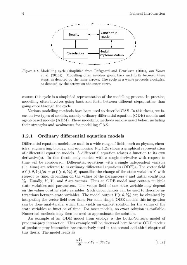
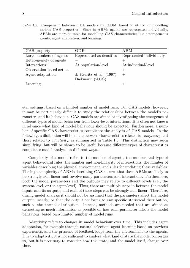
Figure 1.3: Snapshots of simulation runs of the Schelling model of social segregation. (a):For a small value of the tolerance parameter (0.05) the model converges to amixed state in which there is no strong spatial clustering of the two colours. (b):For a larger value of the tolerance parameter the model converges to a segregatedstate in which both colours are clustered into separate neighbourhoods. Thesnapshots were made using the Netlogo implementation of the model (Wilensky1997, 1999).
1.3.1 Detection of tipping points and resilience
ABMs may contain tipping points in parameter space where the model behaviourchanges drastically. For example, predator-prey models like the one in Eq (1.1) oftenfeature tipping points where one or both of the populations go extinct. An ABMexample is the Schelling model of racial segregation (Schelling 1971). In this modelagents of two colours live on a spatial grid, and may choose to change location basedon the proportion of neighbouring agents of the same colour. A ’tolerance’ parameterdescribes the minimum proportion of agents of the same colour each agent findsacceptable. Increasing the value of this parameter causes a transition from a non-segregated state to a segregated state where agents of the same colour form spatialclusters (Fig 1.3). Whereas in the original model version this transition is gradual,in some model versions the state switches suddenly at a precisely determined criticalparameter value (Stauffer and Solomon 2007). Sudden, qualitative switches in modelbehaviour, such as in the latter case, are typical for tipping points.
Since the Schelling model has only few parameters, the parameter value of thetipping point may be estimated by running the model for various parameter values.In contrast, many other ABMs have a large number of parameters, each of whichmay be relevant for detecting the tipping point. Since we have no explicit expressionsthat describe how the model output changes as a function of parameter values, wecannot detect tipping points using bifurcation analysis, as is possible for ODE models.Adaptivity further complicates tipping point detection in ABMs, because the modelbehaviour may continue to change over time rather than to converge to an unchangingsteady state. Also, path dependence ensures that the model may evolve in differentdirections depending on initial conditions or stochastic effects. Currently, there are
10 General Introduction
no reliable methodologies for detecting tipping points in ABMs.A related challenge is the assessment of resilience. Resilience is a system property
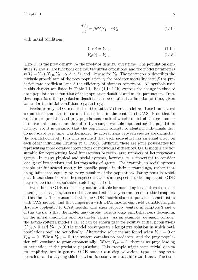
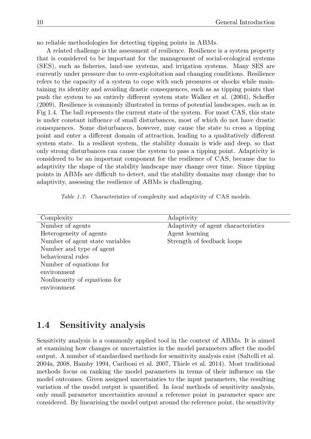
that is considered to be important for the management of social-ecological systems(SES), such as fisheries, land-use systems, and irrigation systems. Many SES arecurrently under pressure due to over-exploitation and changing conditions. Resiliencerefers to the capacity of a system to cope with such pressures or shocks while main-taining its identity and avoiding drastic consequences, such as as tipping points thatpush the system to an entirely different system state Walker et al. (2004), Scheffer(2009). Resilience is commonly illustrated in terms of potential landscapes, such as inFig 1.4. The ball represents the current state of the system. For most CAS, this stateis under constant influence of small disturbances, most of which do not have drasticconsequences. Some disturbances, however, may cause the state to cross a tippingpoint and enter a different domain of attraction, leading to a qualitatively differentsystem state. In a resilient system, the stability domain is wide and deep, so thatonly strong disturbances can cause the system to pass a tipping point. Adaptivity isconsidered to be an important component for the resilience of CAS, because due toadaptivity the shape of the stability landscape may change over time. Since tippingpoints in ABMs are difficult to detect, and the stability domains may change due toadaptivity, assessing the resilience of ABMs is challenging.
Table 1.3: Characteristics of complexity and adaptivity of CAS models.
Complexity AdaptivityNumber of agents Adaptivity of agent characteristicsHeterogeneity of agents Agent learningNumber of agent state variables Strength of feedback loopsNumber and type of agentbehavioural rulesNumber of equations forenvironmentNonlinearity of equations forenvironment
1.4 Sensitivity analysis
Sensitivity analysis is a commonly applied tool in the context of ABMs. It is aimedat examining how changes or uncertainties in the model parameters affect the modeloutput. A number of standardised methods for sensitivity analysis exist (Saltelli et al.2004a, 2008, Hamby 1994, Cariboni et al. 2007, Thiele et al. 2014). Most traditionalmethods focus on ranking the model parameters in terms of their influence on themodel outcomes. Given assigned uncertainties to the input parameters, the resultingvariation of the model output is quantified. In local methods of sensitivity analysis,only small parameter uncertainties around a reference point in parameter space areconsidered. By linearising the model output around the reference point, the sensitivity
Chapter 1 11
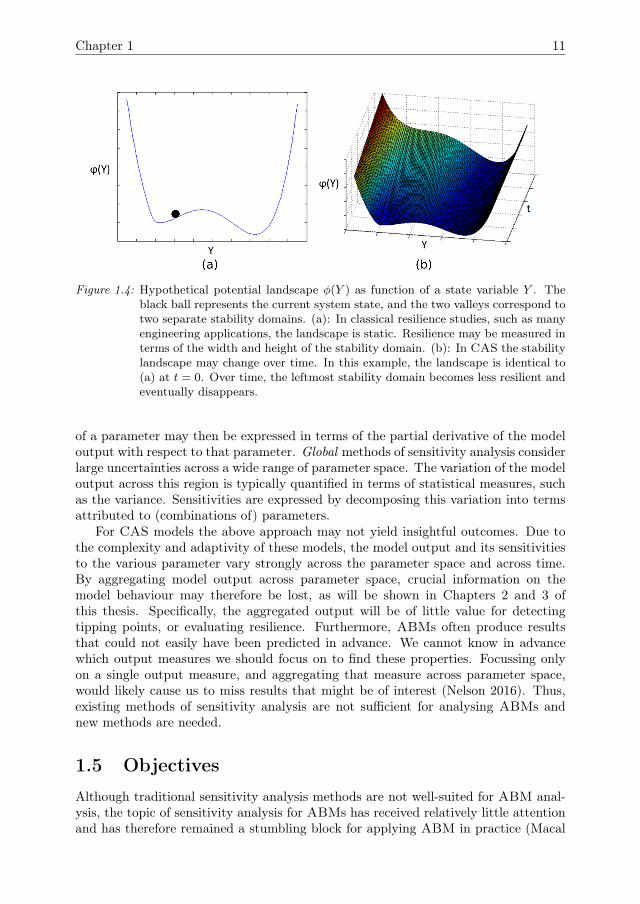
Figure 1.4: Hypothetical potential landscape φ(Y ) as function of a state variable Y . Theblack ball represents the current system state, and the two valleys correspond totwo separate stability domains. (a): In classical resilience studies, such as manyengineering applications, the landscape is static. Resilience may be measured interms of the width and height of the stability domain. (b): In CAS the stabilitylandscape may change over time. In this example, the landscape is identical to(a) at t = 0. Over time, the leftmost stability domain becomes less resilient andeventually disappears.
of a parameter may then be expressed in terms of the partial derivative of the modeloutput with respect to that parameter. Global methods of sensitivity analysis considerlarge uncertainties across a wide range of parameter space. The variation of the modeloutput across this region is typically quantified in terms of statistical measures, suchas the variance. Sensitivities are expressed by decomposing this variation into termsattributed to (combinations of) parameters.
For CAS models the above approach may not yield insightful outcomes. Due tothe complexity and adaptivity of these models, the model output and its sensitivitiesto the various parameter vary strongly across the parameter space and across time.By aggregating model output across parameter space, crucial information on themodel behaviour may therefore be lost, as will be shown in Chapters 2 and 3 ofthis thesis. Specifically, the aggregated output will be of little value for detectingtipping points, or evaluating resilience. Furthermore, ABMs often produce resultsthat could not easily have been predicted in advance. We cannot know in advancewhich output measures we should focus on to find these properties. Focussing onlyon a single output measure, and aggregating that measure across parameter space,would likely cause us to miss results that might be of interest (Nelson 2016). Thus,existing methods of sensitivity analysis are not sufficient for analysing ABMs andnew methods are needed.
1.5 Objectives
Although traditional sensitivity analysis methods are not well-suited for ABM anal-ysis, the topic of sensitivity analysis for ABMs has received relatively little attentionand has therefore remained a stumbling block for applying ABM in practice (Macal
12 General Introduction
2016, Crooks et al. 2008, Filatova et al. 2013). So, there is a need for new sensitivityanalysis methods that are capable of dealing with the complexity of ABMs. Themain aim of this thesis is to develop such methods. Specific issues that we will focuson are,
• The detection of tipping points in ABMs. Detecting tipping points is an im-portant part of ABM analysis. In this thesis, we will examine the possibilitiesof using sensitivity analysis for this purpose. To validate our work, we will alsoapply sensitivity analysis methods to ODE models, where the outcomes can becompared directly to those of bifurcation analysis.
• Analysing adaptivity in ABMs. Adaptivity is an essential component of CAS.The sensitivity analysis methods to be developed in this thesis should allow toanalyse the effects of adaptivity in ABMs.
• Analysing resilience of ABMs. Resilience is considered to be an importantproperty of CAS. Adaptive agents may adjust their behaviour in response topressures, and as such increase the resilience of the system in response to thesepressures. The methods of sensitivity analysis in this thesis should be able toassess the resilience of the system.
1.6 Approach
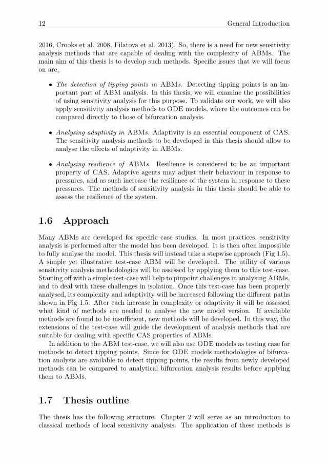
Many ABMs are developed for specific case studies. In most practices, sensitivityanalysis is performed after the model has been developed. It is then often impossibleto fully analyse the model. This thesis will instead take a stepwise approach (Fig 1.5).A simple yet illustrative test-case ABM will be developed. The utility of varioussensitivity analysis methodologies will be assessed by applying them to this test-case.Starting off with a simple test-case will help to pinpoint challenges in analysing ABMs,and to deal with these challenges in isolation. Once this test-case has been properlyanalysed, its complexity and adaptivity will be increased following the different pathsshown in Fig 1.5. After each increase in complexity or adaptivity it will be assessedwhat kind of methods are needed to analyse the new model version. If availablemethods are found to be insufficient, new methods will be developed. In this way, theextensions of the test-case will guide the development of analysis methods that aresuitable for dealing with specific CAS properties of ABMs.
In addition to the ABM test-case, we will also use ODE models as testing case formethods to detect tipping points. Since for ODE models methodologies of bifurca-tion analysis are available to detect tipping points, the results from newly developedmethods can be compared to analytical bifurcation analysis results before applyingthem to ABMs.
1.7 Thesis outline
The thesis has the following structure. Chapter 2 will serve as an introduction toclassical methods of local sensitivity analysis. The application of these methods is
Chapter 1 13
Figure 1.5: The approach in this thesis starts with the analysis of a ’minimal’ CAS. Then,different paths will be followed, increasing (1) its complexity, (2) its adaptivity(2), and (3) both its adaptivity and its complexity.
demonstrated by using them to identify the most influential parameters of an ODEmodel for predator-prey interaction.
Chapter 3 describes the analysis of an ODE predator-prey model that containsseveral tipping points. At these tipping points, the asymptotic behaviour changesbetween stable coexistence, limit cycles, and extinction. It is shown how the presenceof tipping points complicates the interpretation of sensitivity analysis results, andthe use of sensitivity analysis methods for tipping point detection is explored. Thesensitivity analysis results are verified through comparison with analytical resultsfrom bifurcation analysis.
In Chapter 4, an ABM is introduced in which agents compete for a common-pool resource. This ABM serves as a test-case for sensitivity analysis, and althoughit is simple, it still possesses most of the characteristics that complicate sensitivityanalysis of ABMs. Adaptivity is still left out. The model is analysed using threestandard methodologies of sensitivity analysis, and the strengths and weaknesses ofthese methods for analysing ABMs are evaluated.
In Chapter 5, the ABM that was introduced in Chapter 4 is expanded by theinclusion of a mechanism for agent adaptation through a process of natural selection.A sensitivity analysis method to quantify the effects of adaptation over time is devel-oped. Furthermore, it is shown how adaptation affects the resilience of the systemagainst pressures.
In Chapter 6 an extension of the ABM discussed in Chapters 4 and 5 is analysed.In this extension direct interactions are added in the form of cooperation betweenagents. Furthermore, a learning process for individual agents is included for makingdecisions regarding cooperation. It is investigated how various mechanisms affect thelevel of cooperation within the system. Furthermore, it is investigated how coopera-tion affects the resilience of the system.
Chapter 7 concludes with a general discussion. The achievements of this thesisare summarised and discussed. Furthermore, opportunities for further progress areindicated.

Chapter 2
Automated sensitivity analysisfor ecological dynamical models
G.A. ten Broeke, E.H. van Nes, L. Hemerik, G.A.K. van Voorn.To be submitted.
16 Automated sensitivity analysis for ecological dynamical models
Ecological systems are often studied using dynamical models. These models have tobe properly validated in order to be useful. Validation entails the use of data, whichis usually available only for a limited number of variables and short ecological timescales. Such analysis therefore has a strong focus on transient model behaviour.Sensitivity analysis can therefore be a key tool to help this type of model analysis:it quantifies the effects of changes in model parameters and inputs on the modelpredictions, and thus allows for pinpointing influential parameters and inputs aspossible targets for validation experiments. Performing a sensitivity analysis can,however, be costly and cumbersome. In this paper we present a tool in Matlabfor automated sensitivity analysis as an aid for ecological modellers and experi-mentalists. We demonstrate the tool’s performance by comparing its results withsemi-analytical results for two examples. Our study shows that the user-friendlytool quickly yields accurate sensitivities that help in model parametrisation andanalysis.
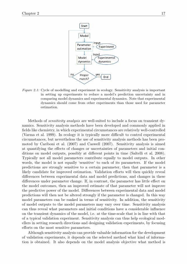
2.1 IntroductionDynamic models are a commonly applied tool to describe key ecological pro-cesses (Gurney and Nisbet 1998). For dynamic models to be of use in ecologicalstudies they should be validated (Augusiak et al. 2014, Rykiel 1996), i.e. it should beevaluated whether the model provides a credible description of the ecological systemit is applied to and whether it is useful for its intended purpose. Validation entails theuse of objective functions (either implicitly through expert judgement, or explicitlythrough statistical measures) to match data to model output. For instance, match-ing model predictions to experimental results is a powerful way to validate models(e.g., McCauley et al. (1999)). Validation is not a one-shot exercise, but a continu-ous process of model evaluation, adaptation, and re-evaluation (Vemer et al. 2013).The ideal modelling cycle therefore entails an iterative loop of matching the modelto (experimental) data, and using the model to generate predictions that steer newexperiments for re-evaluation of the model (Fig 2.1). Usually the modelling cycleincludes parameter estimation, i.e. the setting of model parameter values based onmodel calibration.
A common approach in analysing ecological models is by applying methods forstructural stability analysis. In this approach the focus is on the asymptotic behaviourof the system, i.e. determining the asymptotic system states and their stability underdifferent conditions (Van Nes and Scheffer 2005). Tools are available that can be usedin this approach, such as matcont (Dhooge et al. 2003) and auto07p (Doedel andOldeman 2009) for what is commonly referred to as bifurcation analysis. Structuralstability or bifurcation analysis is for instance useful to assess whether models exhibittipping points. However, for validation it is less suitable, as there is usually a largediscrepancy between the time-scale for the modelled ecological system to evolve toan asymptotic state and the time-scale of validation experiments. Moreover, ecolog-ical systems seldom remain undisturbed for very long. It is therefore important formodel evaluation and validation to consider the transient dynamics, i.e. the ‘modelbehaviour that is not its final behaviour’ (Hastings 2004).
Chapter 2 17
Figure 2.1: Cycle of modelling and experiment in ecology. Sensitivity analysis is importantin setting up experiments to reduce a model’s prediction uncertainty and incomparing model dynamics and experimental dynamics. Note that experimentaldynamics should come from other experiments than those used for parameterestimation.
Methods of sensitivity analysis are well-suited to include a focus on transient dy-namics. Sensitivity analysis methods have been developed and commonly applied infields like chemistry, in which experimental circumstances are relatively well-controlled(Varma et al. 1999). In ecology it is typically more difficult to control experimentalcircumstances, but nevertheless the use of sensitivity analysis methods has been pro-moted by Cariboni et al. (2007) and Caswell (2007). Sensitivity analysis is aimedat quantifying the effects of changes or uncertainties of parameters and initial con-ditions on model outputs, possibly at different points in time (Saltelli et al. 2008).Typically not all model parameters contribute equally to model outputs. In otherwords, the model is not equally ‘sensitive’ to each of its parameters. If the modelpredictions are strongly sensitive to a certain parameter, then that parameter is alikely candidate for improved estimation. Validation efforts will then quickly revealdifferences between experimental data and model predictions, and changes in thesedifferences under parameter change. If, in contrast, the parameter has little effect onthe model outcomes, then an improved estimate of that parameter will not improvethe predictive power of the model. Differences between experimental data and modelpredictions will then not be altered strongly if the parameter is changed. In this waymodel parameters can be ranked in terms of sensitivity. In addition, the sensitivityof model outputs to the model parameters may vary over time. Sensitivity analysiscan thus reveal what parameters and initial conditions have a considerable influenceon the transient dynamics of the model, i.e. at the time-scale that is in line with thatof a typical validation experiment. Sensitivity analysis can thus help ecological mod-ellers in setting research directions and designing validation experiments, by focusingefforts on the most sensitive parameters.
Although sensitivity analysis can provide valuable information for the developmentof validation experiments, it depends on the selected method what kind of informa-tion is obtained. It also depends on the model analysis objective what method is
18 Automated sensitivity analysis for ecological dynamical models
best (Ten Broeke, Van Voorn and Ligtenberg 2016). In general, a crude distinction ismade between local and global methods (Cariboni et al. 2007). Local methods targetspecific points in state and parameter space and thus reveal detailed information thatis valid only in the neighbourhood of the targeted point. Global methods attemptto reveal statistical information that is valid over a larger region, by sampling fromthe full state and parameter space. The latter approach comes at a cost, namely oflosing detailed information on the behaviour of the model that may be of relevancefor validation.
Methods of sensitivity analysis quickly become cumbersome and time-consumingwhen larger models are concerned. For people for whom (statistical) model analysis isnot the primary aim, or who want quick results, this is an undesirable situation thathampers the application of sensitivity analysis. The application range of sensitivityanalysis methodologies is likely to be much broader if automated tools are available.In addition, automated tools are less prone to errors (assuming that the provided inputis according to desired quality standards). Here we present such a tool for performingsensitivity analysis for difference equation (DE) and ordinary differential equation(ODE) models, namely grind for Matlab (http://www.sparcs-center.org/grind).We demonstrate its potential by applying it to two well-known examples, namelya simple difference equation (Ricker 1954) and a classic algae-zooplankton ODEmodel (Rosenzweig and MacArthur 1963), and comparing its results to results ob-tained through semi-analytical methods.
2.2 Local sensitivity analysis
Here we offer a conceptual description of local sensitivity analysis. The mathematicaldetails are given in Appendix 2.A. For the purpose of sensitivity analysis we assumethat the model is a good representation of the modelled system, and there are onlyuncertainties regarding the parameter values, and measurement errors. Local sensi-tivity analysis quantifies the effect of changes in the parameters and initial conditionson the state variables. To perform local sensitivity analysis we first need to establisha default parameter set that functions as a reference point. Ideally, the default setwould be the ‘true’ set of parameter and initial condition values, but in practice thisis usually not the case. Typically we are looking for an improved parameter set andwish to know what parameters should be the focal points of further study.
Starting from the default parameter set, we consider a small change in one of theparameter values. The resulting change in the model outcomes measures the localparameter sensitivity. A large change in outcomes indicates that the parameter isinfluential. To rank the sensitivities, we repeat the same procedure for all modelparameters and initial conditions. Note that usually not all of the model parametershave the same dimensions. To compare the sensitivities of parameters with differentdimensions, they first need to be normalised, for instance by converting them to elas-ticities. Elasticities are dimensionless and straightforward to interpret. For instance,an elasticity of 0.24 means that a 1% change in the input parameter causes a 0.24%change in the output variable.

Chapter 2 19
Table 2.1: Symbols used throughout the text. The upper part contains general symbols, themiddle part symbols for the Ricker model Eq (2.1) and the lower part for theRosenzweig-MacArthur model Eq (2.2).
Symbol Description Units Defaultvalue
ei,j Elasticity of yi to φjf/F Set of odes/desi Index for state variablej Index for parameters and initial conditionsµ Total number of parametersν Total number of state variablesp/P Vector of ode/de parameterssi,j Local sensitivity of yi to φjt/T Time (continuous/discrete)y/Y Vector of state variables of ode/de modely0/Y0 Vector of initial conditions of ode/de modelyi/Yi State variable (i = 1, 2, ..., ν) of ode/de modelφ/Φ Parameters and initial conditions (ode/de)φ̃/Φ̃ Default values of φ/Φc Carrying capacity mg l−1 10N Population density mg l−1 [0,→〉n0 Initial population density mg l−1 0.1q Intraspecific growth rate day−1 0.1A Density of algae mg l−1 [0,→〉a0 Initial density of algae mg l−1 3b Efficiency of food conversion to growth - 0.6g Maximum grazing rate of algae by zooplankton day−1 0.4h Half-saturation algal concentration mg l−1 0.6k Carrying capacity mg l−1 10m Zooplankton background mortality rate day−1 0.15r Relative growth rate day−1 0.5Z Density of zooplankton mg l−1 [0,→〉z0 Initial density of zooplankton mg l−1 3
20 Automated sensitivity analysis for ecological dynamical models
2.2.1 Numerical approximation of local sensitivities
Sensitivities are estimated numerically using the finite differences method. To obtainthis estimate, we first run the model in the default parameter setting. We thenintroduce a small change in one of the parameters, and again run the model. Thedifference between the two runs, relative to the parameter difference, estimates thelocal sensitivity.
The finite differences method requires only one additional model run per param-eter to estimate all of the sensitivities. The method is thus computationally rathercheap and straightforward to apply. grind uses the finite differences method to au-tomatically compute all of the parameter sensitivities or elasticities.
2.2.2 Semi-analytical calculation of local sensitivities
To test the performance of grind in calculating sensitivities we use the semi-analyticalmethod, which can be applied to DE or ODE models. In the semi-analytical methodwe manually, or using symbolic math software (e.g. Matlab Symbolic Math Toolboxor Maple), calculate implicit derivatives of the DEs or ODEs with respect to themodel parameters. These derivatives are expressed as additional difference or dif-ferential equations, to be numerically solved alongside the original model equations.Thus, although only a single model run is needed, the semi-analytic method doesrequire solving additional equations besides the original model equations. Since thesemi-analytic method uses infinitesimal parameter differences, it yields more accurateresults than the numerical method. In practice, however, it is cumbersome and proneto mistakes, especially for models with many state variables and parameters. In thispaper we use the semi-analytical method to check the numerical results obtained bygrind. Note that it is possible in grind to automatically perform the semi-analyticmethod using the Matlab Symbolic Toolbox. To illustrate the principles, we performthe method manually in this paper.
2.3 Examples
Below we discuss the outcomes of the sensitivity analysis for the Ricker model andfor the Rosenzweig-MacArthur model. All of the results were computed in grindand checked semi-analytically. For both models, the results of the two methodsmatched closely. A step-by-step approach for the computations in grind and de-tails of the semi-analytic check are given in Appendix 2.B for the Ricker model andAppendix 2.C.1 for the Rosenzweig-MacArthur model.
2.3.1 Ricker model
The Ricker model of population growth is given as
N(T + 1, n0, q, c) = N(T, n0, q, c)eq(
1−N(T,n0,q,c)c
)(2.1a)
N(T = 0) = n0, (2.1b)
Chapter 2 21
0 20 40 60 80 1000
2
4
6
8
10
Time [days]
n
(a)
0 20 40 60 80 1000
0.2
0.4
0.6
0.8
1
Time [days]
∂n/∂
c*c/
n
(b)
0 20 40 60 80 1000
0.5
1
1.5
2
2.5
3
Time [days]
∂n/∂
q*q/
n
(c)
0 20 40 60 80 1000
0.2
0.4
0.6
0.8
1
Time [days]
∂n/∂
n 0*n0/n
(d)
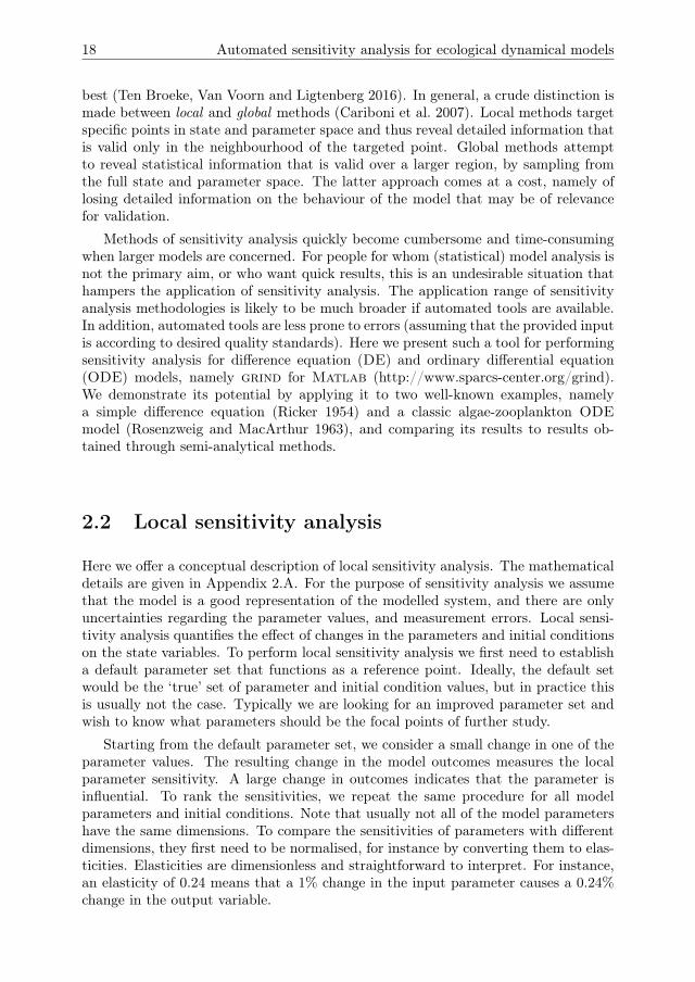
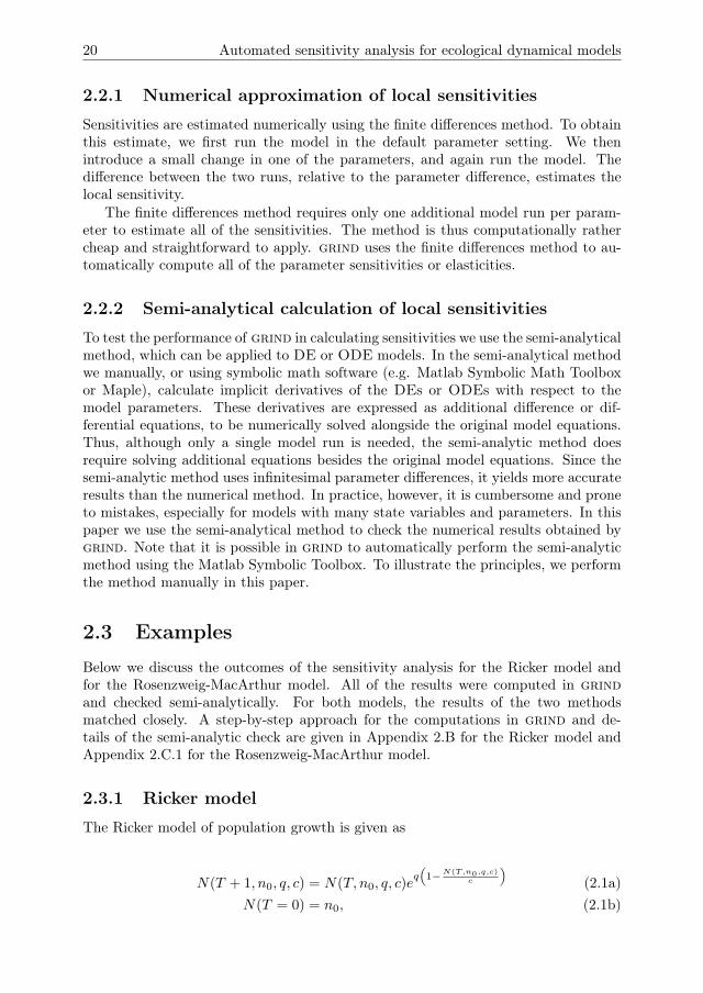
Figure 2.2: Eq (2.1a) and its elasticities in the default parameter set as a function of time,obtained with the ‘timesens’ command in grind. The elasticities show that onlong time scales, c is the only influential parameter. On shorter time scales qand n0 are more influential.
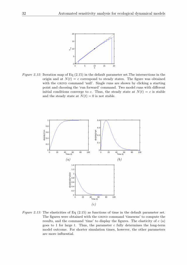
where N(T, n0, q, c) is the population density at time-step T , q is the intraspecificgrowth factor, and c is the carrying capacity. In the following we will drop theparameters from the notation and write N(T ) = N(T, n0, q, c). A sensitivity analysisof the continuous version of the Ricker model, also known as the Pearl-Verhulst orlogistic equation, has been discussed by Banks et al. (2007) and Downing et al. (2013).The population density is estimated by N(T ) in the default parameter set (Fig 2.2a).This population grows towards a steady state value, as is verified by setting N(T ) =N(T + 1) in Eq (2.1a) to determine the steady state solutions: N = 0 and N = c.Analysis using grind shows that N = 0 is unstable and N = c is stable for any q > 0.The model thus converges asymptotically to c for any n0 > 0 and q > 0.
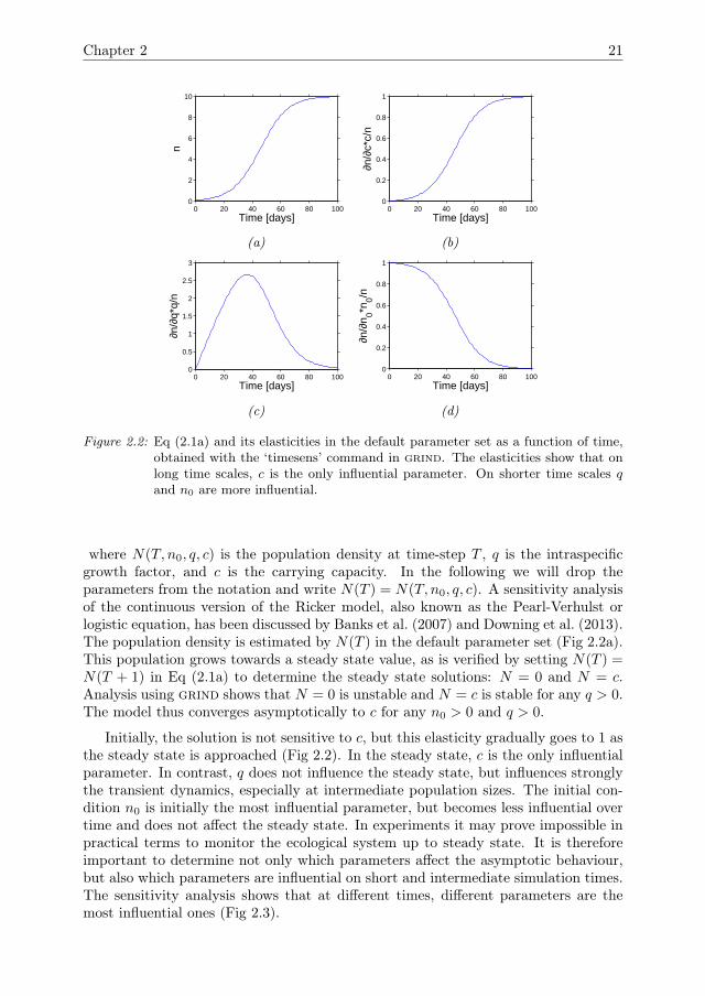
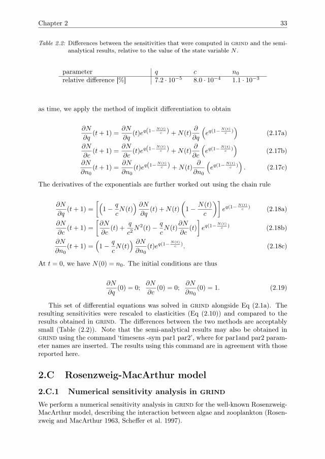
Initially, the solution is not sensitive to c, but this elasticity gradually goes to 1 asthe steady state is approached (Fig 2.2). In the steady state, c is the only influentialparameter. In contrast, q does not influence the steady state, but influences stronglythe transient dynamics, especially at intermediate population sizes. The initial con-dition n0 is initially the most influential parameter, but becomes less influential overtime and does not affect the steady state. In experiments it may prove impossible inpractical terms to monitor the ecological system up to steady state. It is thereforeimportant to determine not only which parameters affect the asymptotic behaviour,but also which parameters are influential on short and intermediate simulation times.The sensitivity analysis shows that at different times, different parameters are themost influential ones (Fig 2.3).
22 Automated sensitivity analysis for ecological dynamical models
(a) (b)
Figure 2.3: Ranking of the elasticities of Eq (2.1a) in the default parameter set at T = 20(a) and T = 100 (b). The results were computed in grind and the graphs weremade in excel. At T = 20 q is the most influential parameter, followed by n0.At T = 100, c is the most influential and the other elasticities are close to zero.
2.3.2 Rosenzweig-MacArthur model
As a second example we consider the well-known Rosenzweig-MacArthur model, de-scribing the interaction between algae and zooplankton (Rosenzweig and MacArthur1963, Scheffer et al. 1997). The population densities depend on the initial conditions,the parameter values, and on time. To simplify the notation we will hereafter writeA = A(a0, z0, r, k, g, h, b,m, t) and similar for Z.
dA
dt= rA
(1− A
k
)− gA
A+ hZ (2.2a)
dZ
dt= b
gA
A+ hZ −mZ (2.2b)
A(0) = a0; Z(0) = z0 (2.2c)
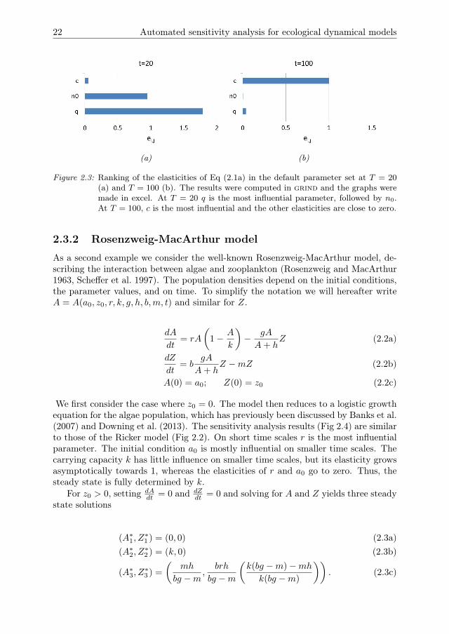
We first consider the case where z0 = 0. The model then reduces to a logistic growthequation for the algae population, which has previously been discussed by Banks et al.(2007) and Downing et al. (2013). The sensitivity analysis results (Fig 2.4) are similarto those of the Ricker model (Fig 2.2). On short time scales r is the most influentialparameter. The initial condition a0 is mostly influential on smaller time scales. Thecarrying capacity k has little influence on smaller time scales, but its elasticity growsasymptotically towards 1, whereas the elasticities of r and a0 go to zero. Thus, thesteady state is fully determined by k.
For z0 > 0, setting dAdt = 0 and dZ
dt = 0 and solving for A and Z yields three steadystate solutions
(A∗1, Z∗1 ) = (0, 0) (2.3a)
(A∗2, Z∗2 ) = (k, 0) (2.3b)
(A∗3, Z∗3 ) =
(mh
bg −m,
brh
bg −m
(k(bg −m)−mh
k(bg −m)
)). (2.3c)
Chapter 2 23
0 5 10 15 200
2
4
6
8
10
Time [days]
A
(a)
0 5 10 15 200
0.2
0.4
0.6
0.8
1
Time [days]
∂A/∂
k
(b)
0 5 10 15 200
0.1
0.2
0.3
0.4
0.5
0.6
0.7
Time [days]
∂A/∂
r
(c)
0 5 10 15 200
0.2
0.4
0.6
0.8
1
Time [days]
∂A/∂
A0
(d)
Figure 2.4: Eq (2.2a) and its local elasticities as functions of time, with z0 = 0. The figureswere obtained with the ‘timesens’ command in grind. In the steady state, kis the only influential parameter, but for shorter simulation times r and a0 areinfluential.
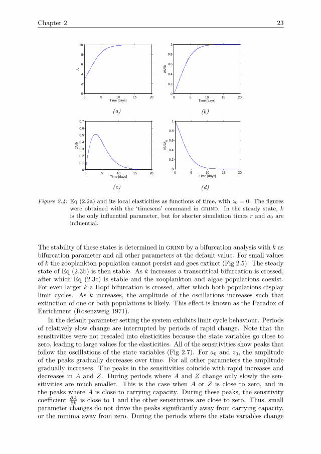
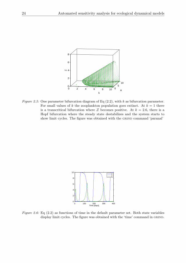
The stability of these states is determined in grind by a bifurcation analysis with k asbifurcation parameter and all other parameters at the default value. For small valuesof k the zooplankton population cannot persist and goes extinct (Fig 2.5). The steadystate of Eq (2.3b) is then stable. As k increases a transcritical bifurcation is crossed,after which Eq (2.3c) is stable and the zooplankton and algae populations coexist.For even larger k a Hopf bifurcation is crossed, after which both populations displaylimit cycles. As k increases, the amplitude of the oscillations increases such thatextinction of one or both populations is likely. This effect is known as the Paradox ofEnrichment (Rosenzweig 1971).
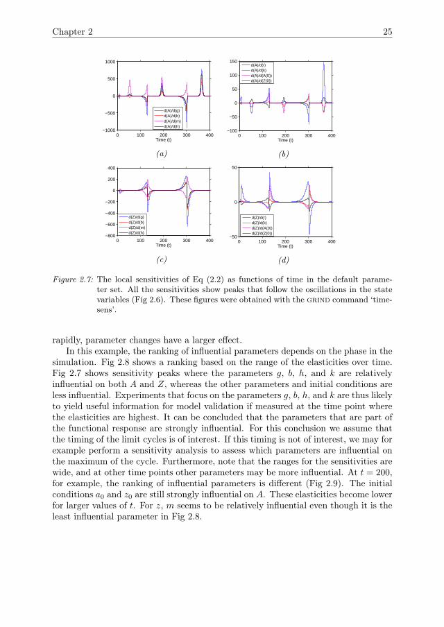
In the default parameter setting the system exhibits limit cycle behaviour. Periodsof relatively slow change are interrupted by periods of rapid change. Note that thesensitivities were not rescaled into elasticities because the state variables go close tozero, leading to large values for the elasticities. All of the sensitivities show peaks thatfollow the oscillations of the state variables (Fig 2.7). For a0 and z0, the amplitudeof the peaks gradually decreases over time. For all other parameters the amplitudegradually increases. The peaks in the sensitivities coincide with rapid increases anddecreases in A and Z. During periods where A and Z change only slowly the sen-sitivities are much smaller. This is the case when A or Z is close to zero, and inthe peaks where A is close to carrying capacity. During these peaks, the sensitivitycoefficient ∂A
∂k is close to 1 and the other sensitivities are close to zero. Thus, smallparameter changes do not drive the peaks significantly away from carrying capacity,or the minima away from zero. During the periods where the state variables change
24 Automated sensitivity analysis for ecological dynamical models
0 2 4 6 8 10 05
100
2
4
6
8
kA
Z
Figure 2.5: One parameter bifurcation diagram of Eq (2.2), with k as bifurcation parameter.For small values of k the zooplankton population goes extinct. At k = 1 thereis a transcritical bifurcation where Z becomes positive. At k = 2.6, there is aHopf bifurcation where the steady state destabilizes and the system starts toshow limit cycles. The figure was obtained with the grind command ‘paranal’
0 100 200 300 4000
2
4
6
8
10
Time [days]
AZ
Figure 2.6: Eq (2.2) as functions of time in the default parameter set. Both state variablesdisplay limit cycles. The figure was obtained with the ‘time’ command in grind.
Chapter 2 25
0 100 200 300 400−1000
−500
0
500
1000
Time (t)
d(A)/d(g)d(A)/d(b)d(A)/d(m)d(A)/d(h)
(a)
0 100 200 300 400−100
−50
0
50
100
150
Time (t)
d(A)/d(r)d(A)/d(k)d(A)/d(A(0))d(A)/d(Z(0))
(b)
0 100 200 300 400−800
−600
−400
−200
0
200
400
Time (t)
d(Z)/d(g)d(Z)/d(b)d(Z)/d(m)d(Z)/d(h)
(c)
0 100 200 300 400−50
0
50
Time (t)
d(Z)/d(r)d(Z)/d(k)d(Z)/d(A(0))d(Z)/d(Z(0))
(d)
Figure 2.7: The local sensitivities of Eq (2.2) as functions of time in the default parame-ter set. All the sensitivities show peaks that follow the oscillations in the statevariables (Fig 2.6). These figures were obtained with the grind command ‘time-sens’.
rapidly, parameter changes have a larger effect.In this example, the ranking of influential parameters depends on the phase in the
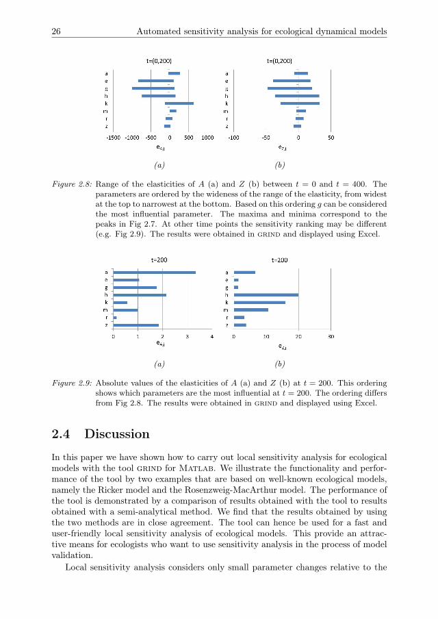
simulation. Fig 2.8 shows a ranking based on the range of the elasticities over time.Fig 2.7 shows sensitivity peaks where the parameters g, b, h, and k are relativelyinfluential on both A and Z, whereas the other parameters and initial conditions areless influential. Experiments that focus on the parameters g, b, h, and k are thus likelyto yield useful information for model validation if measured at the time point wherethe elasticities are highest. It can be concluded that the parameters that are part ofthe functional response are strongly influential. For this conclusion we assume thatthe timing of the limit cycles is of interest. If this timing is not of interest, we may forexample perform a sensitivity analysis to assess which parameters are influential onthe maximum of the cycle. Furthermore, note that the ranges for the sensitivities arewide, and at other time points other parameters may be more influential. At t = 200,for example, the ranking of influential parameters is different (Fig 2.9). The initialconditions a0 and z0 are still strongly influential on A. These elasticities become lowerfor larger values of t. For z, m seems to be relatively influential even though it is theleast influential parameter in Fig 2.8.
26 Automated sensitivity analysis for ecological dynamical models
(a) (b)
Figure 2.8: Range of the elasticities of A (a) and Z (b) between t = 0 and t = 400. Theparameters are ordered by the wideness of the range of the elasticity, from widestat the top to narrowest at the bottom. Based on this ordering g can be consideredthe most influential parameter. The maxima and minima correspond to thepeaks in Fig 2.7. At other time points the sensitivity ranking may be different(e.g. Fig 2.9). The results were obtained in grind and displayed using Excel.
(a) (b)
Figure 2.9: Absolute values of the elasticities of A (a) and Z (b) at t = 200. This orderingshows which parameters are the most influential at t = 200. The ordering differsfrom Fig 2.8. The results were obtained in grind and displayed using Excel.
2.4 Discussion
In this paper we have shown how to carry out local sensitivity analysis for ecologicalmodels with the tool grind for Matlab. We illustrate the functionality and perfor-mance of the tool by two examples that are based on well-known ecological models,namely the Ricker model and the Rosenzweig-MacArthur model. The performance ofthe tool is demonstrated by a comparison of results obtained with the tool to resultsobtained with a semi-analytical method. We find that the results obtained by usingthe two methods are in close agreement. The tool can hence be used for a fast anduser-friendly local sensitivity analysis of ecological models. This provide an attrac-tive means for ecologists who want to use sensitivity analysis in the process of modelvalidation.
Local sensitivity analysis considers only small parameter changes relative to the
Chapter 2 27
default point. Some authors therefore recommend to use global methods (e.g. Cari-boni et al. (2007)), which quantify sensitivities over a larger region of the parameterspace. The aggregation of model outcomes from various samples across a region ofstate and/or parameter space into sample statistics can, however, obscure character-istics of the underlying model behaviour that are relevant for model validation ex-periments (Rakovec et al. 2014), such as the existence of tipping points (van Nes andScheffer 2003, Ten Broeke, Van Voorn and Ligtenberg 2016, Ten Broeke, Van Voorn,Kooi and Molenaar 2016). For example, local sensitivity analysis of the Rosenzweig-MacArthur model gives different outcomes for a parameter setting in which the statevariables converge asymptotically to a positive steady state (Fig 2.7), or to a statewhere the predator is extinct (Fig 2.4). To understand the model behaviour, thesecases should be treated separately, rather than aggregated into a single global sensi-tivity measure.
By identifying which parameters are influential at certain time points during thesimulation, local sensitivity analysis can yield information that is useful for guidingthe design of experiments for model parametrization and validation. For instance, forthe Rosenzweig-MacArthur model our results show that the parameters g, b, h, and kstrongly influence both state variables during peaks in the sensitivities, whereas otherparameters have a much smaller effect. Thus, experiments that focus on these fourparameters and that measure the system during those peaks are likely to yield valuableinformation for model validation. Experiments that focus on other parameters or ondifferent time points do not reveal the same level of detailed information, becauseless influential parameters do not affect the outcomes as much and hence less canbe concluded about (mis)matches between experimental data and model predictions.Our study thus shows that grind helps to obtain useful information for the design ofvalidation experiments in a user-friendly way.
AcknowledgementsWe thank J. Grasman for comments on an earlier version of the manuscript. Theresearch by GTB was financed by the IO/OP theme Complex Adaptive Systems atWageningen University
2.A Local sensitivity analysisWe will consider local sensitivity analysis for two types of dynamic equations that arecommonly used to describe rates of change in ecological processes. These are ordinarydifferential equations (ODEs) and difference equations (DEs). ODEs are given as
dy(t)
dt= f(y(t),p, t) , (2.4)
and DEs as
Y(T + 1) = F(Y(T ),P, T ) , (2.5)
28 Automated sensitivity analysis for ecological dynamical models
where t denotes continuous time, and T denotes discrete time. The vector y re-spectively Y contains state variables, for instance population densities or substanceconcentrations. The vector p respectively P contains parameter values (e.g. in-traspecific growth rate, or carrying capacity). To solve these equations algebraicallyor numerically initial conditions are required (e.g. the population density at the starttime of the experiment), given for ODEs as
y(0) = y0 , (2.6)
and for DEs as
Y(0) = Y0 . (2.7)
For sensitivity analysis we want to express the response of the model to variationsin its parameters or initial conditions. We denote the vector containing parametersand initial conditions as φ = (p,y0) for ODEs and as Φ = (P,Y0) for DEs. A smallchange in any of the parameters or initial conditions to φ̃j + ∆φj corresponds to anew solution yi(φ̃j + ∆φj , t), where the unchanged parameters were omitted from thenotation. The index i (i = 1, 2, ..., ν) can denote any of the state variables, with ν thetotal number of state variables, while index j (j = 1, 2, ..., µ+ν) can denote any of theparameters or initial conditions, with µ the number of parameters. Assuming ∆φj tobe sufficiently small, we estimate the solution with a first order Taylor approximationaround the default solution
yi(φ̃j + ∆φj , t)− yi(φ̃j , t)∆φj
≈ ∂yi(t)
∂φj. (2.8)
Replacing the small letters with capitals, the same expression holds for differenceequations. The right hand side of Eq (2.8) is the local sensitivity coefficient si,j (Varmaet al. 1999)
si,j(t) =∂yi(t)
∂φj(2.9)
which can be evaluated at any time t. If the value of si,j(t) is large, the parameterchange strongly affects the solution. If the value is small, the parameter change haslittle effect.
A drawback of the above local sensitivity coefficient for experimental purposesis that it is not dimensionless. Hence, it is not straightforward to compare localsensitivities of parameters with different dimensions. A dimensionless alternative isthe elasticity, which is obtained by rescaling Eq (2.9)
ei,j(t) =∂yi(t)
∂φj
φjyi(t)
. (2.10)
Chapter 2 29
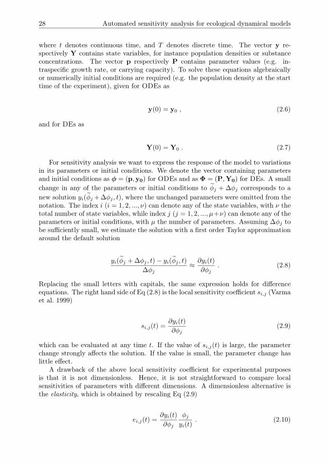
Elasticities may be used to rank parameters in terms of how strongly a relative changein the parameter value affects the model outcomes. For instance, an elasticity of 5means that a 1% change in the input parameter causes a 5% change in the outputvariable. Note that the state variable that is used to scale the elasticity is a function oftime. When comparing elasticities that were computed at different simulation times,it should thus be considered that the scaling factors are different.
2.A.1 Numerical approximation of local sensitivitiesgrind uses the finite differences method to approximate local sensitivities, basedon Eq (2.8). This method has the advantage of not having to solve any additionalequations. If the default solution has been computed, the finite differences methodrequires only one additional model run per sensitivity in order to determine yi(φj +∆φj , t). The sensitivity is then directly computed from the difference between thetwo solutions, as in Eq (2.8).
To accurately estimate the local sensitivity, a small value for ∆φi should be used.To achieve a sufficient level of accuracy grind makes use of the Runge Kutta solver ofMatlab (ode45, with a absolute and relative error of 10−11, Shampine and Reichelt(1997)). By default grind uses for ∆φi a relative disturbance of 10−8 times theoriginal value.
2.A.2 Semi-analytical calculation of local sensitivitiesTo test the performance of grind in calculating sensitivities we use of the semi-analytical method. Consider the partial derivative of Eq (2.4) or Eq (2.5) to parameterφj
d
dt
(∂yi(t, φj)
∂φj
)=∂f(y(t, φj), φj)
∂φj, (2.11)
or for difference equations,
∂Yi(T + 1,Φj)
∂Φj=∂F (Y(T,Φj),Φj)
∂Φj. (2.12)
The state variables y(t) respectively Y (T ) depend not only on time but also on theparameter values. Manually computing the partial derivatives gives an additionaldynamic equation for every state variable. The resulting set of equations is expressedas
d
dt(si,j) =
∂fi∂φj
+
ν∑m=1
∂fi∂ym
sm,j , (2.13)
and equivalent for difference equations. At t = 0 or T = 0, the state variables arefully given by the initial conditions and do not depend on the parameters. The initialconditions are thus
30 Automated sensitivity analysis for ecological dynamical models
si,j(0) =
{1 if φj is the initial condition of yi0 else, (2.14)
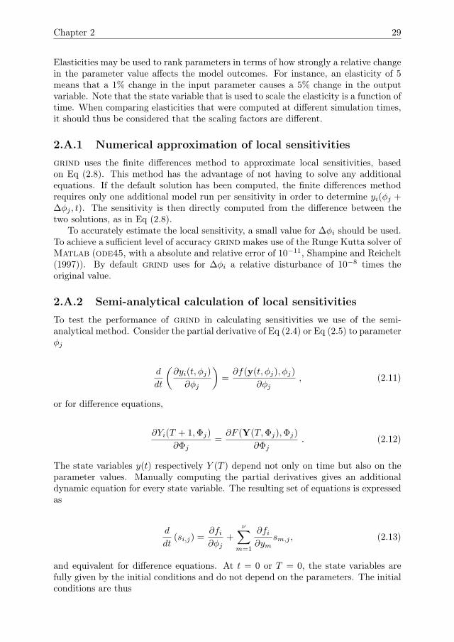
and equivalent for difference equations. The equations for the sensitivities are thensolved alongside the original model equations. This amounts to a total number ofν × (µ + ν) additional equations for all of the sensitivities. The resulting couplednon-linear model can be solved numerically, hence why we refer to this approach assemi-analytical.
2.B Ricker model
2.B.1 Numerical sensitivity analysis in grind
We perform a local sensitivity analysis of the Ricker model in grind. The modelconsists of the difference equation
N(t+ 1, n0, q, c) = N(t, n0, q, c)eq(
1−N(t,n0,q,c)c
), (2.15)
with initial condition
N(0) = n0, (2.16)
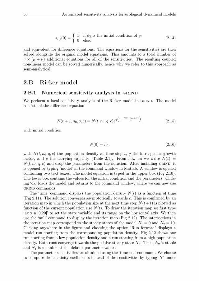
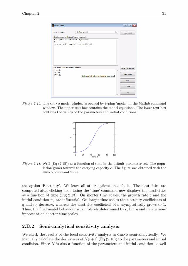
with N(t, n0, q, c) the population density at time-step t, q the intraspecific growthfactor, and c the carrying capacity (Table 2.1). From now on we write N(t) =N(t, n0, q, c) and drop the parameters from the notation. After installing grind, itis opened by typing ‘model’ in the command window in Matlab. A window is openedcontaining two text boxes. The model equation is typed in the upper box (Fig 2.10).The lower box contains the values for the initial condition and the parameters. Click-ing ‘ok’ loads the model and returns to the command window, where we can now usegrind commands.
The ‘time’ command displays the population density N(t) as a function of time(Fig 2.11). The solution converges asymptotically towards c. This is confirmed by aniteration map in which the population size at the next time step N(t+1) is plotted asfunction of the current population size N(t). To draw the iteration map we first type‘ax x n [0,20]’ to set the state variable and its range on the horizontal axis. We thenuse the ‘null’ command to display the iteration map (Fig 2.12). The intersections inthe iteration map correspond to the steady states of the model N1 = 0 and N2 = 10.Clicking anywhere in the figure and choosing the option ’Run forward’ displays amodel run starting from the corresponding population density. Fig 2.12 shows onerun starting from a low population density and a run starting from a high populationdensity. Both runs converge towards the positive steady state N2. Thus, N2 is stableand N1 is unstable at the default parameter values.
The parameter sensitivities are obtained using the ‘timesens’ command. We chooseto compute the elasticity coefficients instead of the sensitivities by typing ‘Y’ under
Chapter 2 31
Figure 2.10: The grind model window is opened by typing ’model’ in the Matlab commandwindow. The upper text box contains the model equations. The lower text boxcontains the values of the parameters and initial conditions.
0 20 40 60 80 1000
2
4
6
8
10
Time (t)
n
Figure 2.11: N(t) (Eq (2.15)) as a function of time in the default parameter set. The popu-lation grows towards the carrying capacity c. The figure was obtained with thegrind command ‘time’.
the option ‘Elasticity’. We leave all other options on default. The elasticities arecomputed after clicking ‘ok’. Using the ‘time’ command now displays the elasticitiesas a function of time (Fig 2.13). On shorter time scales, the growth rate q and theinitial condition n0 are influential. On longer time scales the elasticity coefficients ofq and n0 decrease, whereas the elasticity coefficient of c asymptotically grows to 1.Thus, the final model behaviour is completely determined by c, but q and n0 are moreimportant on shorter time scales.
2.B.2 Semi-analytical sensitivity analysis
We check the results of the local sensitivity analysis in grind semi-analytically. Wemanually calculate the derivatives of N(t+1) (Eq (2.15)) to the parameters and initialcondition. Since N is also a function of the parameters and initial condition as well
32 Automated sensitivity analysis for ecological dynamical models
0 5 10 15 200
5
10
15
20
nn t+
1
Figure 2.12: Iteration map of Eq (2.15) in the default parameter set.The intersections in theorigin and at N(t) = c correspond to steady states. The figure was obtainedwith the grind command ‘null’. Single runs are shown by clicking a startingpoint and choosing the ‘run forward’ command. Two model runs with differentinitial conditions converge to c. Thus, the steady state at N(t) = c is stableand the steady state at N(t) = 0 is not stable.
0 20 40 60 80 1000
0.2
0.4
0.6
0.8
1
Time (t)
d(n)
/d(c
)*c/
n
(a)
0 20 40 60 80 1000
0.1
0.2
0.3
0.4
Time (t)
d(n)
/d(q
)*q/
n
(b)
0 20 40 60 80 1000
0.2
0.4
0.6
0.8
1
1.2
1.4
Time (t)
d(n)
/d(n
(0))
*n(0
)/n
(c)
Figure 2.13: The elasticities of Eq (2.15) as functions of time in the default parameter set.The figures were obtained with the grind command ‘timesens’ to compute theresults, and the command ‘time’ to display the figures. The elasticity of c (a)goes to 1 for large t. Thus, the parameter c fully determines the long-termmodel outcome. For shorter simulation times, however, the other parametersare more influential.
Chapter 2 33
Table 2.2: Differences between the sensitivities that were computed in grind and the semi-analytical results, relative to the value of the state variable N .
parameter q c n0
relative difference [%] 7.2 · 10−5 8.0 · 10−4 1.1 · 10−3
as time, we apply the method of implicit differentiation to obtain
∂N
∂q(t+ 1) =
∂N
∂q(t)eq(1−N(t)
c ) +N(t)∂
∂q
(eq(1−
N(t)c ))
(2.17a)
∂N
∂c(t+ 1) =
∂N
∂c(t)eq(1−N(t)
c ) +N(t)∂
∂c
(eq(1−
N(t)c ))
(2.17b)
∂N
∂n0(t+ 1) =
∂N
∂n0(t)eq(1−N(t)
c ) +N(t)∂
∂n0
(eq(1−
N(t)c )). (2.17c)
The derivatives of the exponentials are further worked out using the chain rule
∂N
∂q(t+ 1) =
[(1− q
cN(t)
) ∂N∂q
(t) +N(t)
(1− N(t)
c
)]eq(1−
N(t)c ) (2.18a)
∂N
∂c(t+ 1) =
[∂N
∂c(t) +
q
c2N2(t)− q
cN(t)
∂N
∂c(t)
]eq(1−
N(t)c ) (2.18b)
∂N
∂n0(t+ 1) =
(1− q
cN(t)
) ∂N∂n0
(t)eq(1−N(t)
c ). (2.18c)
At t = 0, we have N(0) = n0. The initial conditions are thus
∂N
∂q(0) = 0;
∂N
∂c(0) = 0;
∂N
∂n0(0) = 1. (2.19)
This set of differential equations was solved in grind alongside Eq (2.1a). Theresulting sensitivities were rescaled to elasticities (Eq (2.10)) and compared to theresults obtained in grind. The differences between the two methods are acceptablysmall (Table (2.2)). Note that the semi-analytical results may also be obtained ingrind using the command ‘timesens -sym par1 par2’, where for par1and par2 param-eter names are inserted. The results using this command are in agreement with thosereported here.
2.C Rosenzweig-MacArthur model
2.C.1 Numerical sensitivity analysis in grindWe perform a numerical sensitivity analysis in grind for the well-known Rosenzweig-MacArthur model, describing the interaction between algae and zooplankton (Rosen-zweig and MacArthur 1963, Scheffer et al. 1997).
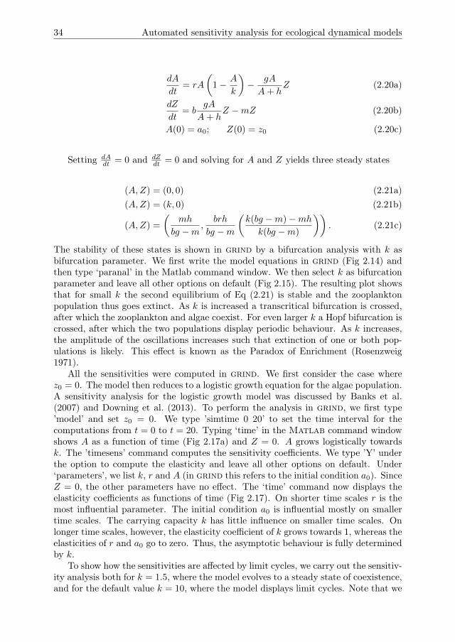
34 Automated sensitivity analysis for ecological dynamical models
dA
dt= rA
(1− A
k
)− gA
A+ hZ (2.20a)
dZ
dt= b
gA
A+ hZ −mZ (2.20b)
A(0) = a0; Z(0) = z0 (2.20c)
Setting dAdt = 0 and dZ
dt = 0 and solving for A and Z yields three steady states
(A,Z) = (0, 0) (2.21a)(A,Z) = (k, 0) (2.21b)
(A,Z) =
(mh
bg −m,
brh
bg −m
(k(bg −m)−mh
k(bg −m)
)). (2.21c)
The stability of these states is shown in grind by a bifurcation analysis with k asbifurcation parameter. We first write the model equations in grind (Fig 2.14) andthen type ‘paranal’ in the Matlab command window. We then select k as bifurcationparameter and leave all other options on default (Fig 2.15). The resulting plot showsthat for small k the second equilibrium of Eq (2.21) is stable and the zooplanktonpopulation thus goes extinct. As k is increased a transcritical bifurcation is crossed,after which the zooplankton and algae coexist. For even larger k a Hopf bifurcation iscrossed, after which the two populations display periodic behaviour. As k increases,the amplitude of the oscillations increases such that extinction of one or both pop-ulations is likely. This effect is known as the Paradox of Enrichment (Rosenzweig1971).
All the sensitivities were computed in grind. We first consider the case wherez0 = 0. The model then reduces to a logistic growth equation for the algae population.A sensitivity analysis for the logistic growth model was discussed by Banks et al.(2007) and Downing et al. (2013). To perform the analysis in grind, we first type’model’ and set z0 = 0. We type ’simtime 0 20’ to set the time interval for thecomputations from t = 0 to t = 20. Typing ‘time’ in the Matlab command windowshows A as a function of time (Fig 2.17a) and Z = 0. A grows logistically towardsk. The ’timesens’ command computes the sensitivity coefficients. We type ’Y’ underthe option to compute the elasticity and leave all other options on default. Under‘parameters’, we list k, r and A (in grind this refers to the initial condition a0). SinceZ = 0, the other parameters have no effect. The ‘time’ command now displays theelasticity coefficients as functions of time (Fig 2.17). On shorter time scales r is themost influential parameter. The initial condition a0 is influential mostly on smallertime scales. The carrying capacity k has little influence on smaller time scales. Onlonger time scales, however, the elasticity coefficient of k grows towards 1, whereas theelasticities of r and a0 go to zero. Thus, the asymptotic behaviour is fully determinedby k.
To show how the sensitivities are affected by limit cycles, we carry out the sensitiv-ity analysis both for k = 1.5, where the model evolves to a steady state of coexistence,and for the default value k = 10, where the model displays limit cycles. Note that we

Chapter 2 35
Figure 2.14: The differential equations for the model (Eq 2.20). The lower text box containsthe initial conditions and parameter values.
Figure 2.15: To perform a bifurcation analysis of the Rosenzweig-MacArthur model ingrind, we select k as bifurcation parameter and leave all other option on de-fault.

36 Automated sensitivity analysis for ecological dynamical models
0 2 4 6 8 10 05
100
2
4
6
8
kA
Z
Figure 2.16: One parameter bifurcation diagram of Eq (2.20), with k as bifurcation param-eter. There is a transcritical bifurcation at k = 1 where Z becomes positive.At k = 2.6, there is a Hopf bifurcation where the steady state destabilizes andthe system starts showing limit cycles. The figure was obtained with the grindcommand ‘paranal’
Table 2.3: The differences between the numerical and the semi-analytical results for thesensitivity coefficients were computed at every time-step. We show the maximumvalue over time for all the combinations of state variables and parameters. Theresults in grind closely match the semi-analytical results.
DeviationA Z
r 2.1 · 10−3 2.1 · 10−4
k 3.6 · 10−3 3.4 · 10−3
g 1.5 · 10−2 5.8 · 10−4
h 1.2 · 10−3 1.0 · 10−4
b 1.1 · 10−3 4.4 · 10−2
m 1.1 · 10−3 1.1 · 10−4
a0 1.2 · 10−3 1.5 · 10−4
z0 3.7 · 10−3 2.2 · 10−4
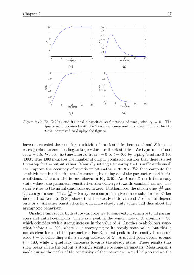
Chapter 2 37
0 5 10 15 200
2
4
6
8
10
Time [days]
A
(a)
0 5 10 15 200
0.1
0.2
0.3
0.4
0.5
0.6
0.7
Time [days]
∂A/∂
r
(b)
0 5 10 15 200
0.2
0.4
0.6
0.8
1
Time [days]
∂A/∂
k
(c)
0 5 10 15 200
0.2
0.4
0.6
0.8
1
Time [days]
∂A/∂
A0
(d)
Figure 2.17: Eq (2.20a) and its local elasticities as functions of time, with z0 = 0. Thefigures were obtained with the ‘timesens’ command in grind, followed by the‘time’ command to display the figures.
have not rescaled the resulting sensitivities into elasticities because A and Z in somecases go close to zero, leading to large values for the elasticities. We type ’model’ andset k = 1.5. We set the time interval from t = 0 to t = 400 by typing ’simtime 0 4004000’. The 4000 indicates the number of output points and ensures that there is a settime-step for the output values. Manually setting a time-step that is sufficiently smallcan improve the accuracy of sensitivity estimates in grind. We then compute thesensitivities using the ’timesens’ command, including all of the parameters and initialconditions. The sensitivities are shown in Fig 2.19. As A and Z reach the steadystate values, the parameter sensitivities also converge towards constant values. Thesensitivities to the initial conditions go to zero. Furthermore, the sensitivities ∂A
∂r and∂A∂k also go to zero. That ∂A
∂k = 0 may seem surprising given the results for the Rickermodel. However, Eq (2.3c) shows that the steady state value of A does not dependon k or r. All other sensitivities have nonzero steady state values and thus affect theasymptotic behaviour.
On short time scales both state variables are to some extent sensitive to all param-eters and initial conditions. There is a peak in the sensitivities of A around t = 30,which coincides with a strong increase in the value of A. Another peak follows some-what before t = 200, where A is converging to its steady state value, but this isnot as clear for all of the parameters. For Z, a first peak in the sensitivities occursclose t = 0, coinciding with a strong decrease of Z. A second peak occurs aroundt = 180, while Z gradually increases towards the steady state. These results thusshow peaks where the output is strongly sensitive to some parameters. Measurementsmade during the peaks of the sensitivity of that parameter would help to reduce the
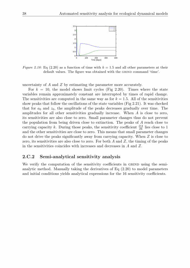
38 Automated sensitivity analysis for ecological dynamical models
0 100 200 300 4000
0.5
1
1.5
2
2.5
3
3.5
Time [days]
AZ
Figure 2.18: Eq (2.20) as a function of time with k = 1.5 and all other parameters at theirdefault values. The figure was obtained with the grind command ‘time’.
uncertainty of A and Z by estimating the parameter more accurately.For k = 10, the model shows limit cycles (Fig 2.20). Times where the state
variables remain approximately constant are interrupted by times of rapid change.The sensitivities are computed in the same way as for k = 1.5. All of the sensitivitiesshow peaks that follow the oscillations of the state variables (Fig 2.21). It was checkedthat for a0 and z0, the amplitude of the peaks decreases gradually over time. Theamplitudes for all other sensitivities gradually increase. When A is close to zero,its sensitivities are also close to zero. Small parameter changes thus do not preventthe population from being driven close to extinction. The peaks of A reach close tocarrying capacity k. During those peaks, the sensitivity coefficient ∂A
∂k lies close to 1and the other sensitivities are close to zero. This means that small parameter changesdo not drive the peaks significantly away from carrying capacity. When Z is close tozero, its sensitivities are also close to zero. For both A and Z, the timing of the peaksin the sensitivities coincides with increases and decreases in A and Z.
2.C.2 Semi-analytical sensitivity analysisWe verify the computation of the sensitivity coefficients in grind using the semi-analytic method. Manually taking the derivatives of Eq (2.20) to model parametersand initial conditions yields analytical expressions for the 16 sensitivity coefficients.
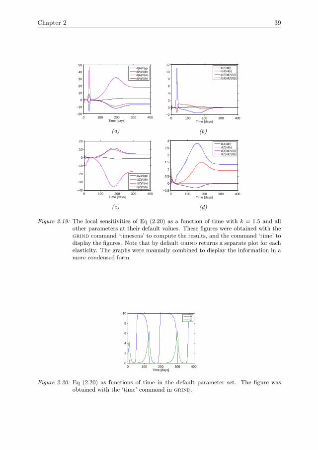
Chapter 2 39
0 100 200 300 400−20
−10
0
10
20
30
40
50
Time [days]
d(A)/d(g)d(A)/d(b)d(A)/d(m)d(A)/d(h)
(a)
0 100 200 300 400−2
0
2
4
6
8
10
12
Time [days]
d(A)/d(r)d(A)/d(k)d(A)/d(A(0))d(A)/d(Z(0))
(b)
0 100 200 300 400−40
−30
−20
−10
0
10
20
Time [days]
d(Z)/d(g)d(Z)/d(b)d(Z)/d(m)d(Z)/d(h)
(c)
0 100 200 300 400−0.5
0
0.5
1
1.5
2
2.5
3
Time [days]
d(Z)/d(r)d(Z)/d(k)d(Z)/d(A(0))d(Z)/d(Z(0))
(d)
Figure 2.19: The local sensitivities of Eq (2.20) as a function of time with k = 1.5 and allother parameters at their default values. These figures were obtained with thegrind command ‘timesens’ to compute the results, and the command ‘time’ todisplay the figures. Note that by default grind returns a separate plot for eachelasticity. The graphs were manually combined to display the information in amore condensed form.
0 100 200 300 4000
2
4
6
8
10
Time [days]
AZ
Figure 2.20: Eq (2.20) as functions of time in the default parameter set. The figure wasobtained with the ‘time’ command in grind.
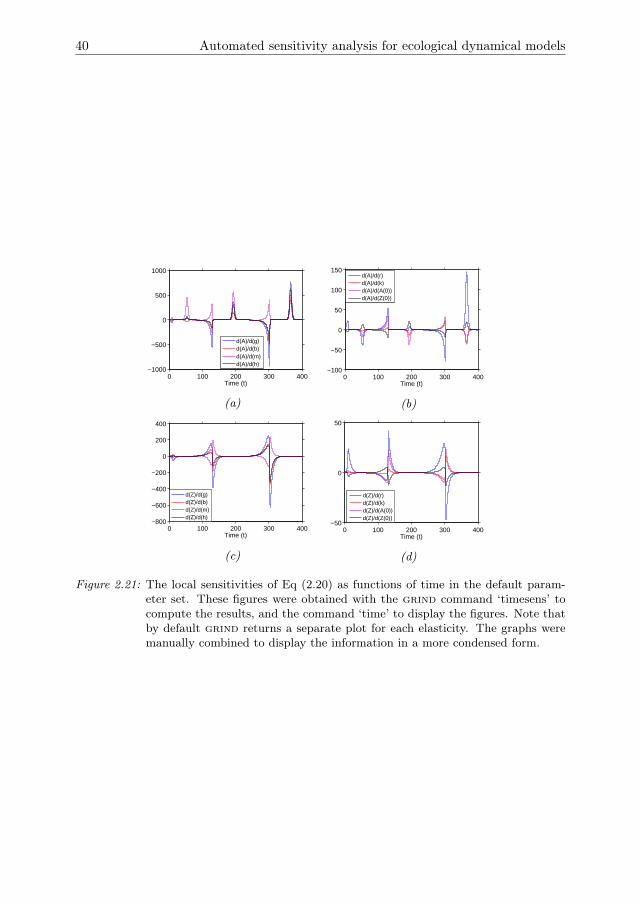
40 Automated sensitivity analysis for ecological dynamical models
0 100 200 300 400−1000
−500
0
500
1000
Time (t)
d(A)/d(g)d(A)/d(b)d(A)/d(m)d(A)/d(h)
(a)
0 100 200 300 400−100
−50
0
50
100
150
Time (t)
d(A)/d(r)d(A)/d(k)d(A)/d(A(0))d(A)/d(Z(0))
(b)
0 100 200 300 400−800
−600
−400
−200
0
200
400
Time (t)
d(Z)/d(g)d(Z)/d(b)d(Z)/d(m)d(Z)/d(h)
(c)
0 100 200 300 400−50
0
50
Time (t)
d(Z)/d(r)d(Z)/d(k)d(Z)/d(A(0))d(Z)/d(Z(0))
(d)
Figure 2.21: The local sensitivities of Eq (2.20) as functions of time in the default param-eter set. These figures were obtained with the grind command ‘timesens’ tocompute the results, and the command ‘time’ to display the figures. Note thatby default grind returns a separate plot for each elasticity. The graphs weremanually combined to display the information in a more condensed form.

Chapter 2 41
d
dt
(∂A
∂r
)= A
(1− A
K
)+ r
(1− 2A
K
)∂A
∂r− gZh
(A+ h)2
∂A
∂r− gA
A+ h
∂Z
∂r(2.22a)
d
dt
(∂Z
∂r
)=
bghZ
(A+ h)2
∂A
∂r+
(bgA
A+ h−m
)∂Z
∂r(2.22b)
d
dt
(∂A
∂K
)= r
(1− 2
A
K
)∂A
∂K+rA2
K2− gZh
(A+ h)2
∂A
∂K− gA
A+ h
∂Z
∂K(2.22c)
d
dt
(∂Z
∂K
)=
bgZh
(A+ h)2
∂A
∂K+
(bgA
A+ h−m
)∂Z
∂K(2.22d)
d
dt
(∂A
∂g
)= r
(1− 2A
K
)∂A
∂g− AZ
A+ h− gZh
(A+ h)2
∂A
∂g− gA
A+ h
∂Z
∂g(2.22e)
d
dt
(∂Z
∂g
)=
bAZ
A+ h+
bgZh
(A+ h)2
∂A
∂g+
(bgA
A+ h−m
)∂Z
∂g(2.22f)
d
dt
(∂A
∂h
)= r
(1− 2A
K
)∂A
∂h+
gAZ
(A+ h)2− ghZ
(A+ h)2
∂A
∂h− gA
A+ h
∂Z
∂h(2.22g)
d
dt
(∂Z
∂h
)=−bgAZ(A+ h)2
+bghZ
(A+ h)2
∂A
∂h+
(bgA
A+ h−m
)∂Z
∂h(2.22h)
d
dt
(∂A
∂b
)= r
(1− 2A
K
)∂A
∂b− ghZ
(A+ h)2
∂A
∂b− gA
A+ h
∂Z
∂b(2.22i)
d
dt
(∂Z
∂b
)=
gAZ
A+ h+
bghZ
(A+ h)2
∂A
∂b+
(bgA
A+ h−m
)∂Z
∂b(2.22j)
d
dt
(∂A
∂m
)= r
(1− 2A
K
)∂A
∂m− ghZ
(A+ h)2
∂A
∂m− gA
A+ h
∂Z
∂m(2.22k)
d
dt
(∂Z
∂m
)=
bghZ
(A+ h)2
∂A
∂m+
(bgA
A+ h−m
)∂Z
∂m− Z (2.22l)
d
dt
(∂A
∂a0
)= r
(1− 2A
K
)∂A
∂a0− ghZ
(A+ h)2
∂A
∂a0− gA
A+ h
∂Z
∂a0(2.22m)
d
dt
(∂Z
∂a0
)=
bghZ
(A+ h)2
∂A
∂a0+
(bgA
A+ h−m
)∂Z
∂a0(2.22n)
d
dt
(∂A
∂z0
)= r
(1− 2A
K
)∂A
∂z0− ghZ
(A+ h)2
∂A
∂z0− gA
A+ h
∂Z
∂z0(2.22o)
d
dt
(∂Z
∂z0
)=
bghZ
(A+ h)2
∂A
∂z0+
(bgA
A+ h−m
)∂Z
∂z0. (2.22p)
The initial conditions for Eq (2.22) are given by Eq (2.14). The set of equations wassolved in grind. The results of this computation match closely with the results thatwere obtained using the grind ‘timesens’ command (Table 2.3).

Chapter 3
Detecting Tipping points inEcological Models withSensitivity Analysis
G.A. ten Broeke, G.A.K. van Voorn, B.W. Kooi, J. Molenaar.Mathematical Modelling of Natural Phenomena 11(4): pp. 47-72.
44 Detecting Tipping points with Sensitivity Analysis
Simulation models are commonly used to understand and predict the developmentof ecological systems, for instance to study the occurrence of tipping points andtheir possible ecological effects. Sensitivity analysis is a key tool in the study ofmodel responses to changes in conditions. The applicability of available method-ologies for sensitivity analysis can be problematic if tipping points are involved.In this paper we demonstrate that not considering these tipping points may resultin misleading statistics on model behaviour. In turn, this limits the applicabil-ity of simulation models in ecological research. Tipping points are best revealedwhen asymptotic model behaviour is considered, i.e. by applying bifurcation anal-ysis. Bifurcation analysis, however, is limited to deterministic dynamic models,whereas many ecological simulation models are nondeterministic and can only beanalysed using sensitivity analysis methodologies. In this paper we explore thepossibilities for applying methodologies of sensitivity analysis to analyse modelswith tipping points. The Bazykin-Berezovskaya model, a deterministic ecologicalmodel of which the structure regarding tipping points is known a priori, is usedas case study. We conclude that important clues about the occurrence of tippingspoints can be revealed from different sensitivity analysis methodologies, if properstatistical and graphical measures are used. The results raise awareness about howtipping points affect temporal model responses in ecological simulation models, andmay also be more generally applicable for nondeterministic models that cannot beanalysed using bifurcation analysis.
3.1 IntroductionEcological researchers and managers of natural systems commonly use simula-tion models to understand and predict the effects of drivers on ecological systems(Schmolke et al. 2010). Most ecological systems are Complex Adaptive Systems withmany interacting, biotic components, and feedbacks (Schlueter et al. 2012). The ap-plicability of simulation models is determined not only by the validity of these models(i.e. whether the models are a proper and useful simplified representation of themodelled system), but also by our ability to analyse them. Model analysis is vitalduring all steps in the development and use of ecological models (Jakeman et al. 2006,Schmolke et al. 2010), including model testing, calibration, validation, uncertaintyestimation, and gaining a better understanding of model behaviour. Reflecting thecomplexity of the modelled system, many simulation models are also of considerablecomplexity. This generates a demand for the development and application of modelanalysis methodologies. Without the right methodologies a proper model analysis isnot possible, and simulation models are of limited use.
We consider two important tools for model analysis, namely sensitivity analysisand bifurcation analysis. Sensitivity analysis quantifies the effects of changes in theparameters (including initial conditions) on the model output (Hamby 1994, Saltelliet al. 2004a, Cariboni et al. 2007, Campolongo et al. 2011). Its main use is to es-timate which parameters are the most influential on certain model outputs. Thisinformation is useful for instance to quantify the information content of data for agiven model, or to establish what parameters to focus on in validation experiments.Bifurcation analysis, on the other hand, considers changes in the topology of the phase
Chapter 3 45
space (i.e. qualitative changes) of the model with changes in parameters (includinginitial conditions). A lack of change in the topology with parameter changes mayindicate resilience, i.e. the capacity of the modelled system to withstand pressureswithout undergoing drastic changes (Walker et al. 2004). Changes in topology mayindicate tipping points that can lead to catastrophic shifts – fast, large-scale, and ir-reversible changes from one system state to another under relatively small changes indrivers (Folke et al. 2004, Scheffer and Carpenter 2003, Scheffer et al. 2009, Boettigeret al. 2013). Tipping points are either bifurcations or separatrices (Guckenheimerand Holmes 2013, Wiggins 1990, Kuznetsov 2004, Seydel 2010). A bifurcation is aspecific parameter setting at which a qualitative change in model behaviour occurs.A separatrix is a manifold in state space that separates two domains of attraction ofneighbouring attractors. In the latter case there are at least two alternative types ofasymptotic model behaviour, and the initial conditions determine to which attractorthe model will eventually evolve if no further manipulations of the system occur.
For many ecological management applications there is an interest in tipping points(Folke et al. 2004) and resilience, i.e. the asymptotic model behavioural features. Forthose applications bifurcation analysis would be the preferred method for analysingmodels. However, the application of bifurcation analysis is restricted by the complex-ity, as well as the type of many ecological models. Bifurcation analysis is well-suitedfor the analysis of deterministic dynamic models (DAEs or differential and algebraicequations) with a limited number of model variables and parameters, for which semi-automated tools are available, such as matcont (Dhooge et al. 2003) and auto07p(Doedel and Oldeman 2009). For complex models with a large number of parame-ters it is often not feasible to analyse the model that way. Furthermore, many typesof models cannot at all be analysed using bifurcation analysis. The reason is thatfor differential equation (ode) models, bifurcation analysis methods rely on the useof derivatives of the model equations, but these are not available for models withstochastic terms, or models where we have no explicit model equations available, suchas agent-based models. Features like tipping points and resilience can neverthelessbe expected in complex ecological simulation models. Therefore there is a dire needfor methodologies that can analyse these models (Crooks et al. 2008, Filatova et al.2013, Levin et al. 2013).
Methodologies of sensitivity analysis may be useful as an alternative for analysingmore complex and nondeterministic ecological models. Sensitivity analysis method-ologies are broadly categorised as being either local or global (Cariboni et al. 2007).Local methodologies quantify the sensitivity at a specific point in parameter space,whereas global quantify it across a range of parameter space. In addition, there arehybrid methodologies (Rakovec et al. 2014, Sobol’ and Kucherenko 2009) that applylocal methodologies at different points in parameter space to obtain a distributionof local sensitivity indices across a range of parameter space. Local methodologieslinearise the output around the point at which they are applied to reveal detailedinformation limited to the neighbourhood of this point, omitting nonlocal interac-tion effects. This linearisation involves the determination of partial derivatives andthus meets the same limitation as bifurcation analysis. Global methodologies, onthe other hand, reveal information that is valid over the full parameter range underinvestigation, by sampling from this range, and thus include nonlocal interaction ef-fects. Model output is typically aggregated into statistical measures across the sample
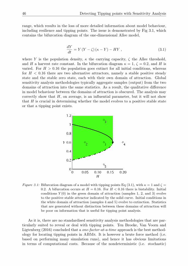
46 Detecting Tipping points with Sensitivity Analysis
range, which results in the loss of more detailed information about model behaviour,including resilience and tipping points. The issue is demonstrated by Fig 3.1, whichcontains the bifurcation diagram of the one-dimensional Allee model,
dY
dt= Y (Y − ζ) (κ− Y )−HY , (3.1)
where Y is the population density, κ the carrying capacity, ζ the Allee threshold,and H a harvest rate constant. In the bifurcation diagram κ = 1, ζ = 0.2, and H isvaried. For H > 0.16 the population goes extinct for all initial conditions, whereasfor H < 0.16 there are two alternative attractors, namely a stable positive steadystate and the stable zero state, each with their own domain of attraction. Globalsensitivity analysis methodologies typically aggregate samples (output) from the twodomains of attraction into the same statistics. As a result, the qualitative differencein model behaviour between the domains of attraction is obscured. The analysis maycorrectly show that H, on average, is an influential parameter, but it will not showthat H is crucial in determining whether the model evolves to a positive stable stateor that a tipping point exists.
Figure 3.1: Bifurcation diagram of a model with tipping points Eq (3.1), with κ = 1 and ζ =0.2. A bifurcation occurs at H = 0.16. For H < 0.16 there is bistability. Initialconditions Y (0) in the green domain of attraction (samples 1, 2, and 3) evolveto the positive stable attractor indicated by the solid curve. Initial conditions inthe white domain of attraction (samples 4 and 5) evolve to extinction. Statisticsthat are generated without distinction between these domains of attraction willbe poor on information that is useful for tipping point analysis.
As it is, there are no standardised sensitivity analysis methodologies that are par-ticularly suited to reveal or deal with tipping points. Ten Broeke, Van Voorn andLigtenberg (2016) concluded that a one-factor-at-a-time approach is the best method-ology for locating tipping points in ABMs. It is however a brute force method (i.e.based on performing many simulation runs), and hence it has obvious limitationsin terms of computational costs. Because of the nondeterministic (i.e. stochastic)
Chapter 3 47
nature of many complex ecological models (including ABMs) many repetitive sim-ulation runs have to be performed at different values of a single parameter before adistinction can be made between effects of tipping points and those of model stochas-ticity. This limits the application value of such sensitivity analysis methodologies forlocating tipping points.
In this paper, we deal with the question of whether methodologies for sensitiv-ity analysis can have a practical use for studying asymptotic features like tippingpoints and resilience in ecological models. By means of an example for which all theasymptotic features can be analysed using bifurcation analysis, we show how muchinformation on tipping points and resilience can be obtained using methodologies forsensitivity analysis. The paper is organised as follows. In Section 3.2 three (groupsof) methodologies for performing sensitivity analysis are discussed. In Section 3.3 thewell-known Bazykin-Berezovskaya predator-prey model is introduced as a case study.The results of the analysis of the test case using sensitivity analysis methodologiesare given in Section 3.4. Section 3.5 contains the discussion and conclusions.
3.2 Sensitivity analysis methodologiesIn this section we provide a general overview of the sensitivity analysis methodologiesthat are applied in this paper. This section can be skipped without loss of readabilityby readers who have extensive knowledge of methodologies for sensitivity analysis, orwho wish to skip the technical details.
3.2.1 Local sensitivity analysisLocal parameter sensitivities are typically expressed as the partial derivative of themodel output with respect to a selected parameter (including initial conditions)
si,j(t) =∂Yj(t)
∂θi, (3.2)
where t is time (i.e. these sensitivities may vary over time), Yj are the output vari-ables, θi the parameters (including initial conditions), i = 1, 2, ..., Np with Np thenumber of parameters, and j = 1, 2, ..., Nv with Nv the number of variables or modeloutputs (see Table 3.1 for an overview of the used symbols). Eq (3.2) may be esti-mated for ode models using the direct differential method (Dickinson and Gelinas1976) (Appendix 3.A). Sensitivity indices are expressed in this method as additionaldifferential equations to be solved alongside the original ode model. Alternatively,finite differences methods can be used to estimate Eq (3.2) based on e.g. the differencebetween a model run in the nominal point and a model run with a slightly differentvalue for the parameter for which the sensitivity is estimated.
In a one-at-a-time sensitivity analysis the local partial derivatives of model out-puts with respect to any number of (preferably all) parameters are determined arounda single point. Local sensitivity indices Eq (3.2) cannot be directly compared becauseparameters may have different units. Therefore, in addition to local sensitivity in-dices one usually reports elasticities, which have been normalised using the nominalparameter values

48 Detecting Tipping points with Sensitivity Analysis
Table 3.1: List of all general symbols used in the paper.
Symbol MeaningA Sampling matrix (used only in Appendix)AB Recombinant sampling matrix (used only in Appendix)B Alternative sampling matrix (used only in Appendix)BA Recombinant sampling matrix (used only in Appendix)E(·) Expected valueei,j Elasticityf Function; model outputG Curve corresponding to global bifurcationg(Y, θ, t) Vector field of ODE model (used only in Appendix)H Curve corresponding to Hopf bifurcationi Index for model parametersJ Jacobian matrixINp Np−dimensional unit hypercube (used only in Appendix)j Index for model outputsl Index for model parametersm Index for model outputsNp Total number of parametersNs Sample size in sampling method by Saltelli et al. (2010)Nv Total number of outputsn Number of samples per parameter in the factorial designP Probability density function (used only in Appendix)Si,j Global first order variance-based sensitivityS̃i,j Global total effect variance-based sensitivitysi,j Local sensitivitys̃i,j delsa local sensitivityt TimeU(·) Uniform probability densityV (·) VarianceVi Partial variance attributed to parameter iW s Stable manifold in state spaceWu Unstable manifold in state spaceY Model output vector with elements YjΘ All parameters θiθi Model parameter or initial condition
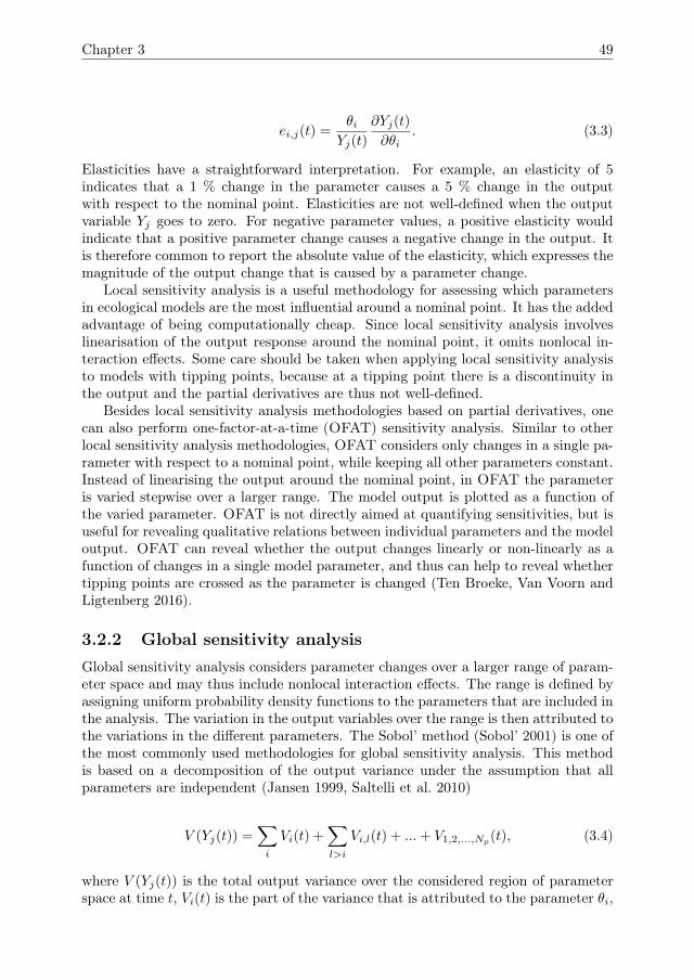
Chapter 3 49
ei,j(t) =θi
Yj(t)
∂Yj(t)
∂θi. (3.3)
Elasticities have a straightforward interpretation. For example, an elasticity of 5indicates that a 1 % change in the parameter causes a 5 % change in the outputwith respect to the nominal point. Elasticities are not well-defined when the outputvariable Yj goes to zero. For negative parameter values, a positive elasticity wouldindicate that a positive parameter change causes a negative change in the output. Itis therefore common to report the absolute value of the elasticity, which expresses themagnitude of the output change that is caused by a parameter change.
Local sensitivity analysis is a useful methodology for assessing which parametersin ecological models are the most influential around a nominal point. It has the addedadvantage of being computationally cheap. Since local sensitivity analysis involveslinearisation of the output response around the nominal point, it omits nonlocal in-teraction effects. Some care should be taken when applying local sensitivity analysisto models with tipping points, because at a tipping point there is a discontinuity inthe output and the partial derivatives are thus not well-defined.
Besides local sensitivity analysis methodologies based on partial derivatives, onecan also perform one-factor-at-a-time (OFAT) sensitivity analysis. Similar to otherlocal sensitivity analysis methodologies, OFAT considers only changes in a single pa-rameter with respect to a nominal point, while keeping all other parameters constant.Instead of linearising the output around the nominal point, in OFAT the parameteris varied stepwise over a larger range. The model output is plotted as a function ofthe varied parameter. OFAT is not directly aimed at quantifying sensitivities, but isuseful for revealing qualitative relations between individual parameters and the modeloutput. OFAT can reveal whether the output changes linearly or non-linearly as afunction of changes in a single model parameter, and thus can help to reveal whethertipping points are crossed as the parameter is changed (Ten Broeke, Van Voorn andLigtenberg 2016).
3.2.2 Global sensitivity analysisGlobal sensitivity analysis considers parameter changes over a larger range of param-eter space and may thus include nonlocal interaction effects. The range is defined byassigning uniform probability density functions to the parameters that are included inthe analysis. The variation in the output variables over the range is then attributed tothe variations in the different parameters. The Sobol’ method (Sobol’ 2001) is one ofthe most commonly used methodologies for global sensitivity analysis. This methodis based on a decomposition of the output variance under the assumption that allparameters are independent (Jansen 1999, Saltelli et al. 2010)
V (Yj(t)) =∑i
Vi(t) +∑l>i
Vi,l(t) + ...+ V1,2,...,Np(t), (3.4)
where V (Yj(t)) is the total output variance over the considered region of parameterspace at time t, Vi(t) is the part of the variance that is attributed to the parameter θi,
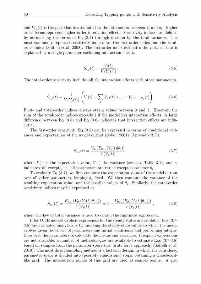
50 Detecting Tipping points with Sensitivity Analysis
and Vi,l(t) is the part that is attributed to the interaction between θi and θl. Higherorder terms represent higher order interaction effects. Sensitivity indices are definedby normalising the terms of Eq (3.4) through division by the total variance. Themost commonly reported sensitivity indices are the first-order index and the total-order index (Saltelli et al. 2008). The first-order index estimates the variance that isexplained by a single parameter excluding interaction effects,
Si,j(t) =Vi(t)
V (Yj(t)). (3.5)
The total-order sensitivity includes all the interaction effects with other parameters,
S̃i,j(t) =1
V (Yj(t))
(Vi(t) +
∑l
Vi,l(t) + ...+ V1,2,...,Np(t)
). (3.6)
First- and total-order indices always attain values between 0 and 1. However, thesum of the total-order indices exceeds 1 if the model has interaction effects. A largedifference between Eq (3.5) and Eq (3.6) indicates that interaction effects are influ-ential.
The first-order sensitivity Eq (3.5) can be expressed in terms of conditional vari-ances and expectations of the model output (Sobol’ 2001) (Appendix 3.D)
Si,j(t) =Vθi(Eθ∼i
(Yj(t)|θi))V (Yj(t))
, (3.7)
where E(·) is the expectation value, V (·) the variance (see also Table 3.1), and ∼indicates ‘all except’, i.e. all parameters are varied except parameter θi.
To evaluate Eq (3.7), we first compute the expectation value of the model outputover all other parameters, keeping θi fixed. We then compute the variance of theresulting expectation value over the possible values of θi. Similarly, the total-ordersensitivity indices may be expressed as
S̃i,j(t) =Eθ∼i
(Vθi(Yj(t)|θ∼i))V (Yj(t))
= 1− Vθ∼i(Eθi(Yj(t)|θ∼i))V (Yj(t))
, (3.8)
where the law of total variance is used to obtain the rightmost expression.If for ODE models explicit expressions for the steady states are available, Eqs (3.7-
3.8) are evaluated analytically by inserting the steady state values to which the modelevolves given the choice of parameters and initial conditions, and performing integra-tions over the parameters to calculate the means and variances. If explicit expressionsare not available, a number of methodologies are available to estimate Eqs (3.7-3.8)based on samples from the parameter space (i.e. brute force approach) (Saltelli et al.2010). The most direct sampling method is a factorial design, in which the consideredparameter space is divided into (possibly equidistant) steps, obtaining a chessboard-like grid. The intersection points of this grid are used as sample points. A grid
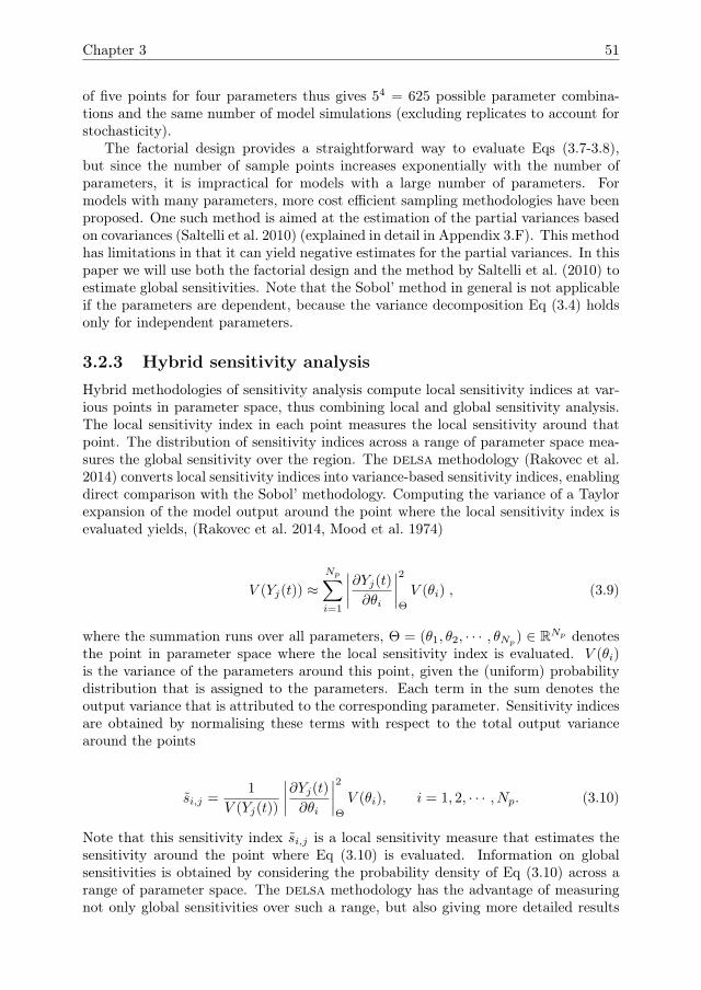
Chapter 3 51
of five points for four parameters thus gives 54 = 625 possible parameter combina-tions and the same number of model simulations (excluding replicates to account forstochasticity).
The factorial design provides a straightforward way to evaluate Eqs (3.7-3.8),but since the number of sample points increases exponentially with the number ofparameters, it is impractical for models with a large number of parameters. Formodels with many parameters, more cost efficient sampling methodologies have beenproposed. One such method is aimed at the estimation of the partial variances basedon covariances (Saltelli et al. 2010) (explained in detail in Appendix 3.F). This methodhas limitations in that it can yield negative estimates for the partial variances. In thispaper we will use both the factorial design and the method by Saltelli et al. (2010) toestimate global sensitivities. Note that the Sobol’ method in general is not applicableif the parameters are dependent, because the variance decomposition Eq (3.4) holdsonly for independent parameters.
3.2.3 Hybrid sensitivity analysisHybrid methodologies of sensitivity analysis compute local sensitivity indices at var-ious points in parameter space, thus combining local and global sensitivity analysis.The local sensitivity index in each point measures the local sensitivity around thatpoint. The distribution of sensitivity indices across a range of parameter space mea-sures the global sensitivity over the region. The delsa methodology (Rakovec et al.2014) converts local sensitivity indices into variance-based sensitivity indices, enablingdirect comparison with the Sobol’ methodology. Computing the variance of a Taylorexpansion of the model output around the point where the local sensitivity index isevaluated yields, (Rakovec et al. 2014, Mood et al. 1974)
V (Yj(t)) ≈Np∑i=1
∣∣∣∣∂Yj(t)∂θi
∣∣∣∣2Θ
V (θi) , (3.9)
where the summation runs over all parameters, Θ = (θ1, θ2, · · · , θNp) ∈ RNp denotes
the point in parameter space where the local sensitivity index is evaluated. V (θi)is the variance of the parameters around this point, given the (uniform) probabilitydistribution that is assigned to the parameters. Each term in the sum denotes theoutput variance that is attributed to the corresponding parameter. Sensitivity indicesare obtained by normalising these terms with respect to the total output variancearound the points
s̃i,j =1
V (Yj(t))
∣∣∣∣∂Yj(t)∂θi
∣∣∣∣2Θ
V (θi), i = 1, 2, · · · , Np. (3.10)
Note that this sensitivity index s̃i,j is a local sensitivity measure that estimates thesensitivity around the point where Eq (3.10) is evaluated. Information on globalsensitivities is obtained by considering the probability density of Eq (3.10) across arange of parameter space. The delsa methodology has the advantage of measuringnot only global sensitivities over such a range, but also giving more detailed results
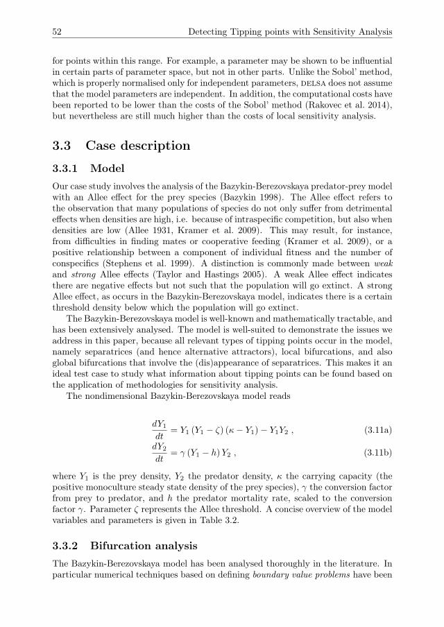
52 Detecting Tipping points with Sensitivity Analysis
for points within this range. For example, a parameter may be shown to be influentialin certain parts of parameter space, but not in other parts. Unlike the Sobol’ method,which is properly normalised only for independent parameters, delsa does not assumethat the model parameters are independent. In addition, the computational costs havebeen reported to be lower than the costs of the Sobol’ method (Rakovec et al. 2014),but nevertheless are still much higher than the costs of local sensitivity analysis.
3.3 Case description
3.3.1 Model
Our case study involves the analysis of the Bazykin-Berezovskaya predator-prey modelwith an Allee effect for the prey species (Bazykin 1998). The Allee effect refers tothe observation that many populations of species do not only suffer from detrimentaleffects when densities are high, i.e. because of intraspecific competition, but also whendensities are low (Allee 1931, Kramer et al. 2009). This may result, for instance,from difficulties in finding mates or cooperative feeding (Kramer et al. 2009), or apositive relationship between a component of individual fitness and the number ofconspecifics (Stephens et al. 1999). A distinction is commonly made between weakand strong Allee effects (Taylor and Hastings 2005). A weak Allee effect indicatesthere are negative effects but not such that the population will go extinct. A strongAllee effect, as occurs in the Bazykin-Berezovskaya model, indicates there is a certainthreshold density below which the population will go extinct.
The Bazykin-Berezovskaya model is well-known and mathematically tractable, andhas been extensively analysed. The model is well-suited to demonstrate the issues weaddress in this paper, because all relevant types of tipping points occur in the model,namely separatrices (and hence alternative attractors), local bifurcations, and alsoglobal bifurcations that involve the (dis)appearance of separatrices. This makes it anideal test case to study what information about tipping points can be found based onthe application of methodologies for sensitivity analysis.
The nondimensional Bazykin-Berezovskaya model reads
dY1
dt= Y1 (Y1 − ζ) (κ− Y1)− Y1Y2 , (3.11a)
dY2
dt= γ (Y1 − h)Y2 , (3.11b)
where Y1 is the prey density, Y2 the predator density, κ the carrying capacity (thepositive monoculture steady state density of the prey species), γ the conversion factorfrom prey to predator, and h the predator mortality rate, scaled to the conversionfactor γ. Parameter ζ represents the Allee threshold. A concise overview of the modelvariables and parameters is given in Table 3.2.
3.3.2 Bifurcation analysis
The Bazykin-Berezovskaya model has been analysed thoroughly in the literature. Inparticular numerical techniques based on defining boundary value problems have been
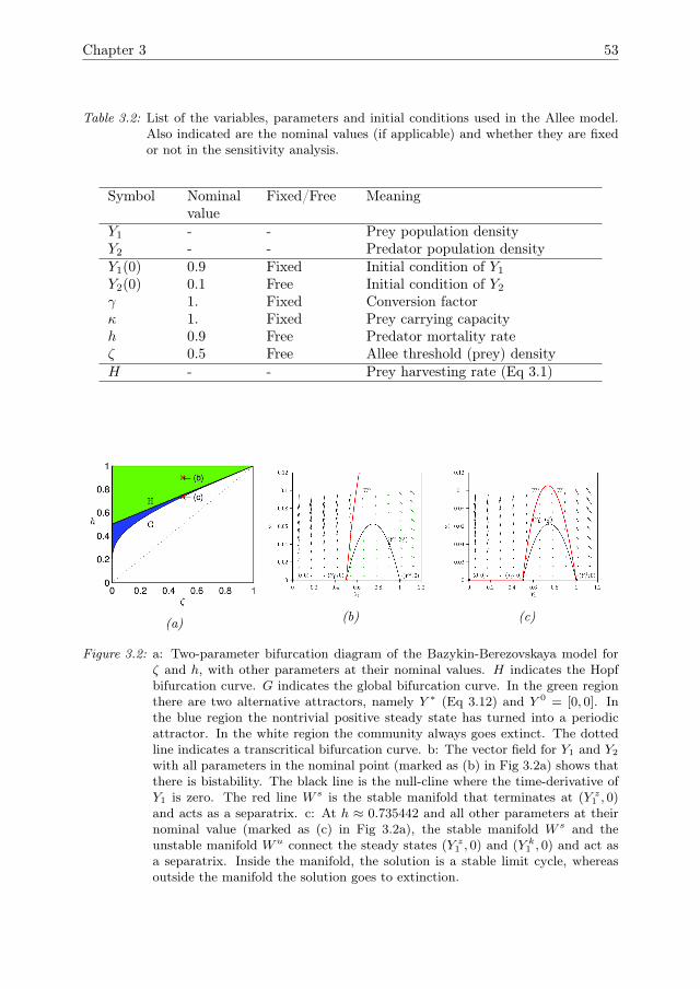
Chapter 3 53
Table 3.2: List of the variables, parameters and initial conditions used in the Allee model.Also indicated are the nominal values (if applicable) and whether they are fixedor not in the sensitivity analysis.
Symbol Nominalvalue
Fixed/Free Meaning
Y1 - - Prey population densityY2 - - Predator population densityY1(0) 0.9 Fixed Initial condition of Y1
Y2(0) 0.1 Free Initial condition of Y2
γ 1. Fixed Conversion factorκ 1. Fixed Prey carrying capacityh 0.9 Free Predator mortality rateζ 0.5 Free Allee threshold (prey) densityH - - Prey harvesting rate (Eq 3.1)
(a) (b) (c)
Figure 3.2: a: Two-parameter bifurcation diagram of the Bazykin-Berezovskaya model forζ and h, with other parameters at their nominal values. H indicates the Hopfbifurcation curve. G indicates the global bifurcation curve. In the green regionthere are two alternative attractors, namely Y ∗ (Eq 3.12) and Y 0 = [0, 0]. Inthe blue region the nontrivial positive steady state has turned into a periodicattractor. In the white region the community always goes extinct. The dottedline indicates a transcritical bifurcation curve. b: The vector field for Y1 and Y2
with all parameters in the nominal point (marked as (b) in Fig 3.2a) shows thatthere is bistability. The black line is the null-cline where the time-derivative ofY1 is zero. The red line W s is the stable manifold that terminates at (Y z1 , 0)and acts as a separatrix. c: At h ≈ 0.735442 and all other parameters at theirnominal value (marked as (c) in Fig 3.2a), the stable manifold W s and theunstable manifold Wu connect the steady states (Y z1 , 0) and (Y k1 , 0) and act asa separatrix. Inside the manifold, the solution is a stable limit cycle, whereasoutside the manifold the solution goes to extinction.
54 Detecting Tipping points with Sensitivity Analysis
used to localize a heteroclinic point-to-point connection (Van Voorn et al. 2007).This connection is not structurally stable, and has a biological interpretation as over-exploitation. We summarise these results for convenience before proceeding to thesensitivity analysis.
Eq (3.11) has four steady state solutions, three trivial ones (Y 0 = [0, 0], Y z = [ζ, 0],Y k = [κ, 0]), and a nontrivial one
Y ∗ = [h , hζ − κ ζ − h2 + hκ] . (3.12)
The Jacobian matrix for the nontrivial steady state is
J|Y=Y ∗ =
(h (ζ + κ− 2h) −h
γ (h− κ) (ζ − h) 0
). (3.13)
The determinant of J is used to determine the transcritical bifurcation of thenontrivial steady state, i.e. the point where the predator species can enter the systemand sustain itself. The trace is used to determine the Hopf bifurcation, i.e. the pointwhere the nontrivial stable steady state becomes unstable and periodic behaviourappears, giving rise to (in this case stable) limit cycles.
The bifurcation diagram displayed in Fig 3.2a shows the asymptotic behaviour ofthe model as function of ζ and h (γ = 1, κ = 1). Three transcritical bifurcations arefound at h0 = 0, hz = ζ, and hk = κ, and the Hopf bifurcation occurs at
hH = 12 (κ+ ζ) , (3.14)
which is indicated by the curve H in Fig 3.2a. The model displays bistability fora significant part of parameter space. When the nontrivial steady state is positive,there exists a unique manifold that terminates at the trivial steady state Y z and actsas a separatrix (Fig 3.2b). Initial conditions on the right hand side of the separatrixconverge to Y ∗ and on the left hand side to the trivial steady state Y 0. Thus, in thegreen parameter region in Fig 3.2a the model may converge to the nontrivial steadystate Y ∗, or to the trivial steady state Y 0, depending on the initial conditions. In theblue parameter region the model may converge either to the limit cycle around Y ∗,or to Y 0.
The heteroclinic point-to-point connection links the saddle steady state Y k to thesaddle steady state Y z, as the stable manifold Ws belonging to Y z overlaps withthe unstable manifold Wu belonging to Y k (see Fig 3.2c for the connection at theparameter set ζ = 0.5, hG ≈ 0.735442). The two-parameter continuation of thiscurve, indicated by G in Fig 3.2a, is obtained by using auto(Doedel and Oldeman2009) with a set of boundary conditions (Van Voorn et al. 2007, 2010). For values ofh > hG (green and blue parameter regions) the system displays bistability. For valuesh < hG the separatrix has disappeared, and Y 0 is the sole attractor (white parameterregion).
Chapter 3 55
3.4 Results of sensitivity analysisIn this section we apply the sensitivity analysis methodologies that are presentedin Section 3.2 to the Bazykin-Berezovskaya model and discuss the obtained results.We consider only the predator density Y2 as model output and parameters h andζ as inputs to demonstrate the principles. The parameters γ and κ are fixed atthe nominal values, and Y1(0) is fixed such that its value lies between κ = 1 andthe highest sampled value of ζ. Note, that for the sensitivity analysis we assume aresearcher who is aware that tipping points may exist, but who is not able for whateverreason to perform bifurcation analysis. The aim is to evaluate which of the sensitivityanalysis methodologies can be useful in detecting, or revealing clues about, tippingpoints such as the transcritical bifurcation, the Hopf bifurcation, the separatrix andthe heteroclinic connection.
3.4.1 Results of local sensitivity analysis
A classical starting point of a sensitivity analysis is to quantify the local sensitivitiesEq (3.2) as given in subsection 3.2.1. For finite values of t we use the direct differentialmethod (Appendix 3.A) to determine these local sensitivities (details of the calculationare given in Appendix 3.B). The results show that the predator density initially ismost sensitive to the initial condition Y2(0), which is an obvious result (Fig 3.3). Asthe simulation proceeds, the sensitivity to Y2(0) decreases to zero, while the sensitivityto h becomes the largest. The elasticities show the same outcome: the sensitivity ofthe model for Y2(0) decreases to zero, while the sensitivity for h becomes the largest.
For long simulation times (effectively t→∞) the model and its parameter sensi-tivities evolve to steady state values. The steady state sensitivities can also be deter-mined analytically by taking the derivative in the positive steady state Y ∗ Eq (3.12),
s∗ζ =∂Y ∗2∂ζ
= h− κ , (3.15)
s∗h =∂Y ∗2∂h
= κ+ ζ − 2h , (3.16)
and
s∗Y2(0) = 0, (3.17)
where the index j in Eq (3.2) is dropped from the notation, and for the index i wewrite ζ, h, or Y2(0). Table 3.3 gives these steady state sensitivities, along with theassociated elasticities Eq (3.3). The outcomes show a close match with those in Fig 3.3for sufficiently large values of t.
Note that the above results estimate the effects of small parameter changes aroundthe nominal point. For larger parameter changes with respect to the nominal set,tipping points and other nonlinearities may become important, in which case theseresults are no longer valid. For example, whereas sY2(0) = 0 in the nominal setting, Fig
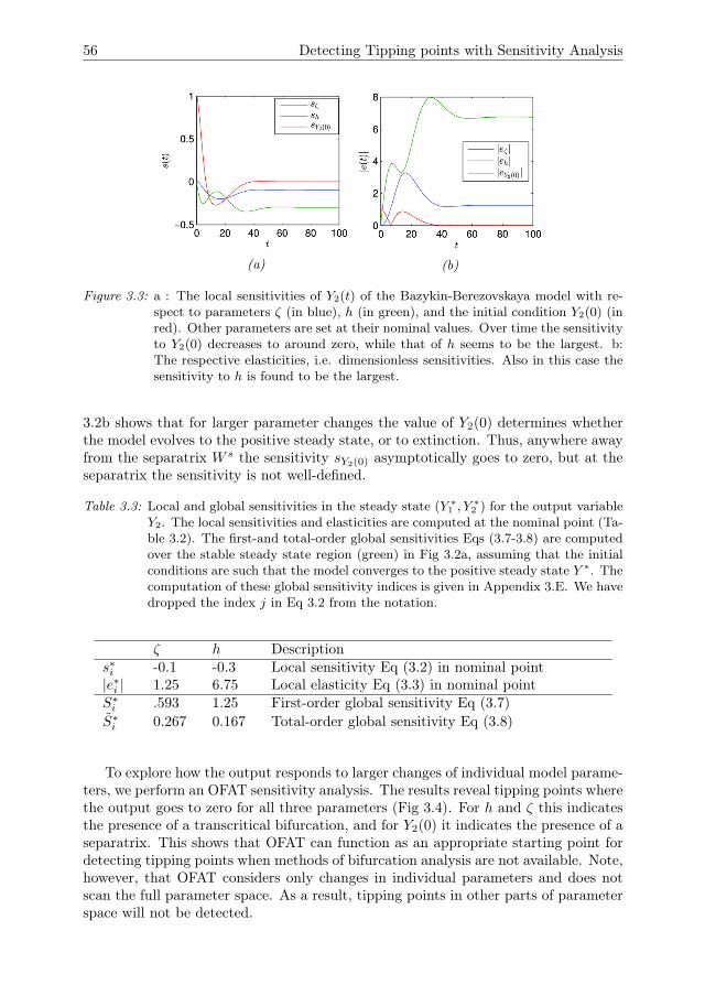
56 Detecting Tipping points with Sensitivity Analysis
(a) (b)
Figure 3.3: a : The local sensitivities of Y2(t) of the Bazykin-Berezovskaya model with re-spect to parameters ζ (in blue), h (in green), and the initial condition Y2(0) (inred). Other parameters are set at their nominal values. Over time the sensitivityto Y2(0) decreases to around zero, while that of h seems to be the largest. b:The respective elasticities, i.e. dimensionless sensitivities. Also in this case thesensitivity to h is found to be the largest.
3.2b shows that for larger parameter changes the value of Y2(0) determines whetherthe model evolves to the positive steady state, or to extinction. Thus, anywhere awayfrom the separatrix W s the sensitivity sY2(0) asymptotically goes to zero, but at theseparatrix the sensitivity is not well-defined.
Table 3.3: Local and global sensitivities in the steady state (Y ∗1 , Y
∗2 ) for the output variable
Y2. The local sensitivities and elasticities are computed at the nominal point (Ta-ble 3.2). The first-and total-order global sensitivities Eqs (3.7-3.8) are computedover the stable steady state region (green) in Fig 3.2a, assuming that the initialconditions are such that the model converges to the positive steady state Y ∗. Thecomputation of these global sensitivity indices is given in Appendix 3.E. We havedropped the index j in Eq 3.2 from the notation.
ζ h Descriptions∗i -0.1 -0.3 Local sensitivity Eq (3.2) in nominal point|e∗i | 1.25 6.75 Local elasticity Eq (3.3) in nominal pointS∗i .593 1.25 First-order global sensitivity Eq (3.7)S̃∗i 0.267 0.167 Total-order global sensitivity Eq (3.8)
To explore how the output responds to larger changes of individual model parame-ters, we perform an OFAT sensitivity analysis. The results reveal tipping points wherethe output goes to zero for all three parameters (Fig 3.4). For h and ζ this indicatesthe presence of a transcritical bifurcation, and for Y2(0) it indicates the presence of aseparatrix. This shows that OFAT can function as an appropriate starting point fordetecting tipping points when methods of bifurcation analysis are not available. Note,however, that OFAT considers only changes in individual parameters and does notscan the full parameter space. As a result, tipping points in other parts of parameterspace will not be detected.
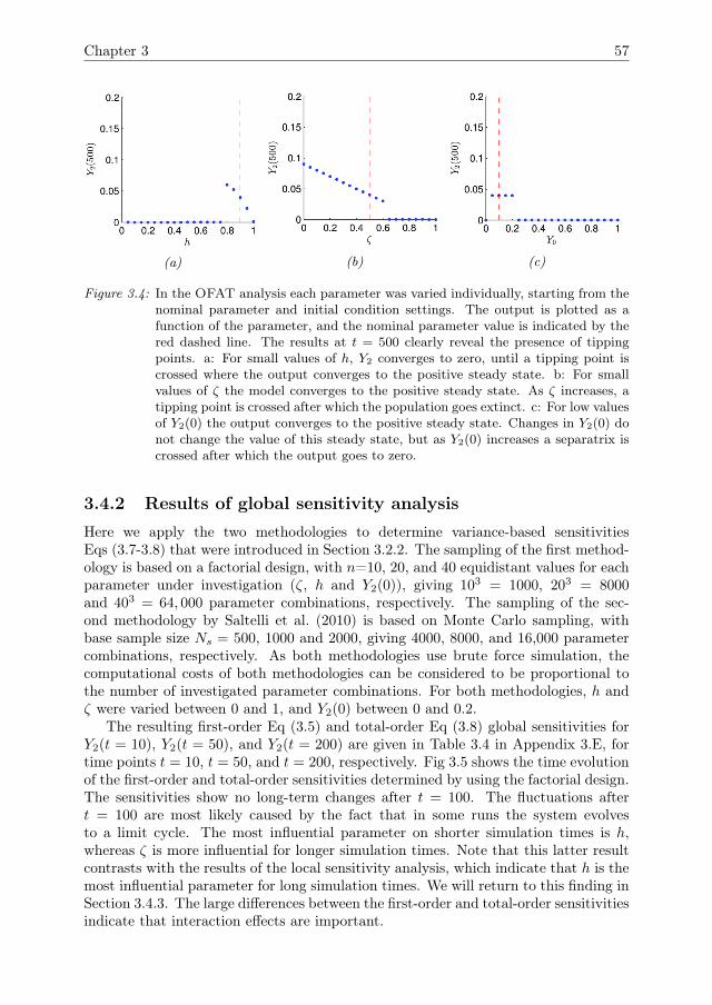
Chapter 3 57
(a) (b) (c)
Figure 3.4: In the OFAT analysis each parameter was varied individually, starting from thenominal parameter and initial condition settings. The output is plotted as afunction of the parameter, and the nominal parameter value is indicated by thered dashed line. The results at t = 500 clearly reveal the presence of tippingpoints. a: For small values of h, Y2 converges to zero, until a tipping point iscrossed where the output converges to the positive steady state. b: For smallvalues of ζ the model converges to the positive steady state. As ζ increases, atipping point is crossed after which the population goes extinct. c: For low valuesof Y2(0) the output converges to the positive steady state. Changes in Y2(0) donot change the value of this steady state, but as Y2(0) increases a separatrix iscrossed after which the output goes to zero.
3.4.2 Results of global sensitivity analysis
Here we apply the two methodologies to determine variance-based sensitivitiesEqs (3.7-3.8) that were introduced in Section 3.2.2. The sampling of the first method-ology is based on a factorial design, with n=10, 20, and 40 equidistant values for eachparameter under investigation (ζ, h and Y2(0)), giving 103 = 1000, 203 = 8000and 403 = 64, 000 parameter combinations, respectively. The sampling of the sec-ond methodology by Saltelli et al. (2010) is based on Monte Carlo sampling, withbase sample size Ns = 500, 1000 and 2000, giving 4000, 8000, and 16,000 parametercombinations, respectively. As both methodologies use brute force simulation, thecomputational costs of both methodologies can be considered to be proportional tothe number of investigated parameter combinations. For both methodologies, h andζ were varied between 0 and 1, and Y2(0) between 0 and 0.2.
The resulting first-order Eq (3.5) and total-order Eq (3.8) global sensitivities forY2(t = 10), Y2(t = 50), and Y2(t = 200) are given in Table 3.4 in Appendix 3.E, fortime points t = 10, t = 50, and t = 200, respectively. Fig 3.5 shows the time evolutionof the first-order and total-order sensitivities determined by using the factorial design.The sensitivities show no long-term changes after t = 100. The fluctuations aftert = 100 are most likely caused by the fact that in some runs the system evolvesto a limit cycle. The most influential parameter on shorter simulation times is h,whereas ζ is more influential for longer simulation times. Note that this latter resultcontrasts with the results of the local sensitivity analysis, which indicate that h is themost influential parameter for long simulation times. We will return to this finding inSection 3.4.3. The large differences between the first-order and total-order sensitivitiesindicate that interaction effects are important.
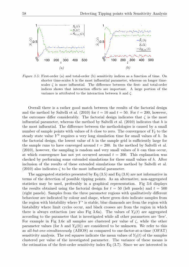
58 Detecting Tipping points with Sensitivity Analysis
(a) (b)
Figure 3.5: First-order (a) and total-order (b) sensitivity indices as a function of time. Onshorter time-scales h is the most influential parameter, whereas on longer time-scales ζ is more influential. The difference between the first- and total-orderindices shows that interaction effects are important. A large portion of thevariance is attributed to the interaction between h and ζ.
Overall there is a rather good match between the results of the factorial designand the method by Saltelli et al. (2010) for t = 10 and t = 50. For t = 200, however,the outcomes differ considerably. The factorial design indicates that ζ is the mostinfluential parameter, whereas the method by Saltelli et al. (2010) indicates that h isthe most influential. The difference between the methodologies is caused by a smallnumber of sample points with values of h close to zero. The convergence of Y2 to thesteady state value Y 0 requires a very long simulation time for small values of h. Inthe factorial design, the lowest value of h in the sample grid is sufficiently large forthe sample runs to have converged around t = 200. In the method by Saltelli et al.(2010), however, the sampling is random and very small values of h can thus occur,at which convergence has not yet occurred around t = 200. This explanation waschecked by performing some extended simulations for these small values of h. Afterinclusion of the results of these extended simulations the method by Saltelli et al.(2010) also indicates ζ to be the most influential parameter.
The aggregated statistics presented by Eq (3.5) and Eq (3.8) are not informative interms of the detection of possible tipping points. As an alternative, non-aggregatedstatistics may be used, preferably in a graphical representation. Fig 3.6 displaysthe results obtained using the factorial design for t = 50 (left panels) and t = 500(right panels). Samples from the three parameter regions with qualitatively differentbehaviour are indicated by colour and shape, where green dots indicate samples fromthe region with bistability where Y ∗ is stable, blue diamonds are from the region withbistability where limit cycles occur, and black crosses are from the region in whichthere is always extinction (see also Fig 3.6a). The values of Y2(t) are aggregatedaccording to the parameter that is investigated while all other parameters are ‘free’.For example in Fig 3.6c all samples are clustered per value of ζ, while the otherparameter values (for h and Y2(0)) are considered to be unknown. We refer to thisas all-but-one-simultaneously (ABOS) as compared to one-factor-at-a-time (OFAT)sensitivity analysis. The red squares indicate the mean values of Y2(t) of the samplesclustered per value of the investigated parameter. The variance of these means isthe estimation of the first-order sensitivity index Eq (3.7). Since we are interested in
Chapter 3 59
revealing tipping points where the model evolves to extinction, we plot the minimumvalue of the limit cycle for samples that show limit cycles.
Based on the graphical ABOS results in Fig 3.6c parameter ζ can be consideredto be the most influential at t = 50. The decreasing mean (i.e. red squares) withincreasing value of ζ corresponds to the decreasing green parameter region on whichbistability occurs (compare to Fig 3.2a and Fig 3.6a). The cloud of black crosses is dueto the fact that at t = 50 the model still displays considerable transient behaviour. Fort = 500 the transient behaviour has disappeared and the means are near zero for ζ >0.5 (Fig 3.6d), while also the diversity in values of Y2(t) decreases for increasing valuesof ζ. It can be concluded from this figure that the region of bistability decreases forincreasing values of ζ, i.e. ζ is an influential parameter in determining the bistabilityin the model.
In Fig 3.6e the ABOS of parameter h at t = 50 is displayed. The samples fromthe green parameter region are limited to h > 0.5, and furthermore the nonzero valuesof Y2(t) increase for decreasing values of h. This is in accordance with the bifurcationdiagram in Fig 3.6a. Starting from the right, the means increase then decrease, untilaround h = 0.5 the means become zero. This is a strong indication of a tippingpoint around this value of h. Indeed, in Fig 3.6b the one-parameter continuationcurve of Y ∗ as function of h is displayed (obtained using auto (Doedel and Oldeman2009)), where ζ = 0.5. Within the range 0.75 < h < 1 the positive steady state isstable, while within 0.5 < h < 0.75 it is unstable. After the destabilization at theHopf bifurcation at h = 0.75 the heteroclinic bifurcation occurs at h ≈ 0.735442, andthen the transcritical bifurcation at h = 0.5. The means in Fig 3.6f seem to followthe one-parameter continuation curve of Y ∗ rather faithfully. In addition, nearingthe transcritical bifurcation there is a marked increase in variance. The nonzerotransient behaviour is limited to very low values of h. This is explained by the longsimulation time that is required for the system to evolve to Y 0 for small values ofh. When t = 500 the increase in variance is less pronounced, while the ‘spike’ ofblack crosses has disappeared. One may suspect the existence of bistability based onthe existence of two separate clouds (namely the green and the blue ones) and thedivergence between the green cloud and the red means for decreasing h. Althoughfor 0.5 < h < 0.75 the values of the positive samples increase with decreasing h, themeans decrease because a larger number of samples converges to extinction.
The sensitivity of the model to the initial condition Y2(0) is shown in Fig 3.6g att = 50 and Fig 3.6h at t = 500. From both figures it can be concluded that Y2(0)does not contribute considerably to the model output. While for t = 50 there is stilla cloud of black crosses, at t = 500 this has disappeared. The means however do notvary considerably as function of Y2(0), which corresponds to the earlier findings thatY2(0) is not an influential parameter.
3.4.3 Results of hybrid sensitivity analysis
The delsa methodology combines aspects of local and global sensitivity analysis andis aimed at obtaining more detailed information on the distribution of the sensitivityindices at specific point. In this case, we would like to include points from the threeparameter regions in which qualitatively different behaviour occurs (see Fig 3.2a). Foreach point in the factorial design, the local sensitivity is estimated using the direct
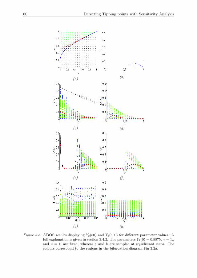
60 Detecting Tipping points with Sensitivity Analysis
(a) (b)
(c) (d)
(e) (f)
(g) (h)
Figure 3.6: ABOS results displaying Y2(50) and Y2(500) for different parameter values. Afull explanation is given in section 3.4.2. The parameters Y1(0) = 0.9875, γ = 1.,and κ = 1. are fixed, whereas ζ and h are sampled at equidistant steps. Thecolours correspond to the regions in the bifurcation diagram Fig 3.2a.
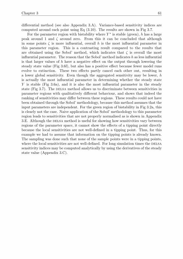
Chapter 3 61
differential method (see also Appendix 3.A). Variance-based sensitivity indices arecomputed around each point using Eq (3.10). The results are shown in Fig 3.7.
For the parameter region with bistability where Y ∗ is stable (green), h has a largepeak around 1 and ζ around zero. From this it can be concluded that althoughin some points ζ is more influential, overall h is the most influential parameter inthis parameter region. This is a contrasting result compared to the results thatare obtained using the Sobol’ method, which indicates that ζ is overall the mostinfluential parameter. The reason that the Sobol’ method indicates h as less influentialis that larger values of h have a negative effect on the output through lowering thesteady state value (Fig 3.6f), but also has a positive effect because fewer model runsevolve to extinction. These two effects partly cancel each other out, resulting ina lower global sensitivity. Even though the aggregated sensitivity may be lower, his actually the most influential parameter in determining whether the steady stateY is stable (Fig 3.6a), and it is also the most influential parameter in the steadystate (Fig 3.7). The delsa method allows us to discriminate between sensitivities inparameter regions with qualitatively different behaviour, and shows that indeed theranking of sensitivities may differ between these regions. These results could not havebeen obtained through the Sobol’ methodology, because this method assumes that theinput parameters are independent. For the green region of bistability in Fig 3.2a, thisis clearly not the case. Naive application of the Sobol’ methodology to this parameterregion leads to sensitivities that are not properly normalised as is shown in Appendix3.E. Although the delsa method is useful for showing how sensitivities vary betweenregions of the parameter space, it cannot show the effects of a tipping point directlybecause the local sensitivities are not well-defined in a tipping point. Thus, for thisexample we had to assume that information on the tipping points is already known.The sampling was done such that none of the sample points were in a tipping points,where the local sensitivities are not well-defined. For long simulation times the delsasensitivity indices may be computed analytically by using the derivatives of the steadystate value (Appendix 3.C).
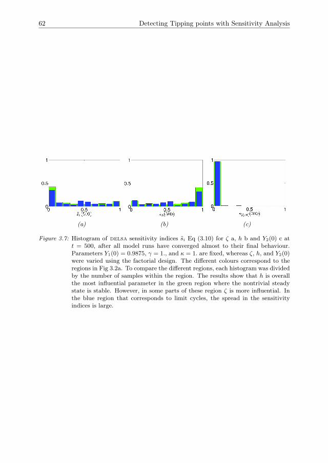
62 Detecting Tipping points with Sensitivity Analysis
(a) (b) (c)
Figure 3.7: Histogram of delsa sensitivity indices s̃i Eq (3.10) for ζ a, h b and Y2(0) c att = 500, after all model runs have converged almost to their final behaviour.Parameters Y1(0) = 0.9875, γ = 1., and κ = 1. are fixed, whereas ζ, h, and Y2(0)were varied using the factorial design. The different colours correspond to theregions in Fig 3.2a. To compare the different regions, each histogram was dividedby the number of samples within the region. The results show that h is overallthe most influential parameter in the green region where the nontrivial steadystate is stable. However, in some parts of these region ζ is more influential. Inthe blue region that corresponds to limit cycles, the spread in the sensitivityindices is large.
Chapter 3 63
3.5 Discussion & Conclusions
The usefulness of simulation models for studying tipping points and resilience in eco-logical systems is limited by the availability of suitable methodologies for model anal-ysis. Bifurcation analysis is the preferred methodology for detecting tipping points indeterministic models, but cannot be applied to other types of simulation models. Theresults in this paper show that sensitivity analysis methodologies can be useful to ob-tain information on tipping points in ecological models. Furthermore, it is shown thata combination of different methodologies for sensitivity analysis increases the amountof information on possible tipping points in ecological models. Below we discuss thepossibilities and limitations of each of the applied methodologies in more detail.
Local sensitivity analysis is a useful methodology for assessing which parameters inecological models are the most influential around a nominal point. This methodologyconsiders only the linear response of the output. It is thus not well-suited for detectingtipping points. A local analysis can be extended as a one-factor-at-a-time (OFAT)analysis (Ten Broeke, Van Voorn and Ligtenberg 2016), in which the sensitivity ofthe model to a certain parameter is investigated by going stepwise through parameterspace, where at each parameter value simulation is used to determine the model out-put. In effect this methodology can be considered as a discrete, brute force analogueto bifurcation analysis. Note, that since OFAT does not scan the full parameterspace, it may not detect all tipping points. By including more than one parameterin the OFAT analysis the probability of detecting other tipping points (if there areany) increases. The costs of OFAT are typically not such that the inclusion of otherparameters becomes prohibitively computationally expensive. In this paper, we showthat OFAT can reveal separatrices and transcritical bifurcations. In Ten Broeke,Van Voorn and Ligtenberg (2016) it was shown that OFAT can be applied to detecttipping points in non-ODE models with a comparable level of success.
Global sensitivity analysis evaluates parameter sensitivities by aggregating modeloutput across parameter space. Time-dependent global sensitivity analysis can beused to gain insight into the dynamics of a model and to suggest parameters for moredetailed investigation. In our example, time-dependent global sensitivity analysisshows that the global sensitivities continue to show oscillations on long simulationtimes, which indicates that some samples display limit cycles. Given that other sam-ples evolve to a stable steady state, this indicates the existence of a Hopf bifurcation.However, standard global sensitivity analysis methodologies do not consider qualita-tive changes of the underlying model behaviour. As a result, these methodologiescan give misleading outcomes in the presence of tipping points (van Nes and Scheffer2003). In our test-case the Sobol’ indices indicate ζ as the most influential param-eter. However, h is more influential in determining whether the model converges tothe positive steady state (Figs 3.2a and 3.6), and also on the value of the steady state(Fig 3.7). The reason that the Sobol’ approach leads to a misleading conclusion isthat an increase in h has a positive effect on the mean output because fewer sam-ple points converge to extinction, but also has a negative effect because value of thepositive steady state is lowered. This information is revealed by applying a samplingdesign that allows for the calculation of (discrete) conditional means and that has suf-ficient coverage, e.g. the factorial design we use in this paper, combined with a propergraphical representation (Fig 3.6). Sparser sampling designs, such as the design in
64 Detecting Tipping points with Sensitivity Analysis
Saltelli et al. (2008) have the negative side-effect that critical information about tip-ping points is lost. If the goal is to locate tipping points, we thus recommend to adopta proper sampling design and data representation. Ideally such a design would scanthe entire parameter space, like the factorial design, but this is often not possiblein practice due to the computational expense. For larger parameter spaces, a goodsampling design may retain the characteristic of the ABOS method that the modeloutput is evaluated at a number of values for certain (combinations) of parameters,while keeping all other parameters constant. Such an approach allows to (graphically)isolate the effects of the investigated parameters as in Fig 3.6 and gives better insightinto how these combinations of parameters affect the output, including the possiblepresence of tipping points. A further limitation of the Sobol’ method is its reliance onthe assumption that the model parameters are independent. This assumption is notalways reasonable for ecological models, where certain parameter combinations maynot make sense in terms of the ecological assumptions behind the model, or when wewant to quantify sensitivities separately for subregions of parameter space.
Hybrid methodologies of sensitivity analysis give a good overview of the globalparameter sensitivities (Rakovec et al. 2014). Furthermore, these methodologies arewell-suited for the computation of parameter sensitivities for subregions within theparameter space. Thus, if the approximate location of tipping points in parameterspace is known, hybrid methodologies of sensitivity analysis can be used to identifyinfluential parameters for separate types of model behaviour, as was done in Fig 3.7for the Bazykin-Berezovskaya model. A limitation of hybrid methodologies is thatthey do not seem to reveal information about the location of tipping points. For thattask a different approach should be followed.
The results in this paper show that global methodologies of sensitivity analysismay yield misleading results when naively applied across the full parameter space ofa model that contains tipping points. When methods of bifurcation analysis are ap-plicable, these can be used to detect bifurcations before global sensitivity analysis isapplied. Should tipping points be found, then we suggest to separate parameter space(and possibly state space) based on the location(s) of the tipping point(s) and performseparate sensitivity analysis for the different regions. This way the obtained resultsare more informative regarding the sensitivity of the model to the different inputs.For models that cannot be analysed using bifurcation analysis, sensitivity analysismethodologies can yield some information on the possible existence of tipping points.Specifically, we suggest the use of OFAT as a starting point to gain information about(the location of) tipping points. Since OFAT does not scan the full parameter space,ideally it is supplemented by a global method of sensitivity analysis to investigateinteraction effects. Here we used a factorial design, which scans the full parameterspace, and combined with a graphical representation as in Fig 3.6, can also be usedgain information about tipping points. We have shown that well-known methodologycan still be applied to systems with tipping points - which are in fact the most inter-esting ones in ecology -, provided that they are combined with a thorough insight inthe bifurcation structure of the system. In line with the ’curse of dimensionality’ wealso admit that a complete analysis of systems with a high number of dimensions stillmeets with some practical limitations and can be considered an open problem. Thisopen issue is part of ongoing research.
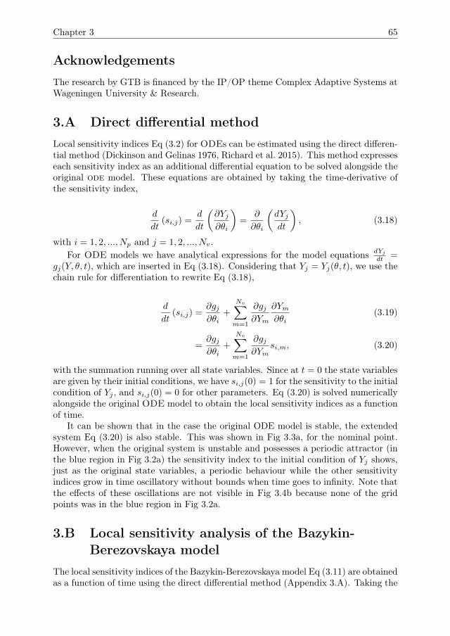
Chapter 3 65
AcknowledgementsThe research by GTB is financed by the IP/OP theme Complex Adaptive Systems atWageningen University & Research.
3.A Direct differential methodLocal sensitivity indices Eq (3.2) for ODEs can be estimated using the direct differen-tial method (Dickinson and Gelinas 1976, Richard et al. 2015). This method expresseseach sensitivity index as an additional differential equation to be solved alongside theoriginal ode model. These equations are obtained by taking the time-derivative ofthe sensitivity index,
d
dt(si,j) =
d
dt
(∂Yj∂θi
)=
∂
∂θi
(dYjdt
), (3.18)
with i = 1, 2, ..., Np and j = 1, 2, ..., Nv.For ODE models we have analytical expressions for the model equations dYj
dt =gj(Y, θ, t), which are inserted in Eq (3.18). Considering that Yj = Yj(θ, t), we use thechain rule for differentiation to rewrite Eq (3.18),
d
dt(si,j) =
∂gj∂θi
+
Nv∑m=1
∂gj∂Ym
∂Ym∂θi
(3.19)
=∂gj∂θi
+
Nv∑m=1
∂gj∂Ym
si,m, (3.20)
with the summation running over all state variables. Since at t = 0 the state variablesare given by their initial conditions, we have si,j(0) = 1 for the sensitivity to the initialcondition of Yj , and si,j(0) = 0 for other parameters. Eq (3.20) is solved numericallyalongside the original ODE model to obtain the local sensitivity indices as a functionof time.
It can be shown that in the case the original ODE model is stable, the extendedsystem Eq (3.20) is also stable. This was shown in Fig 3.3a, for the nominal point.However, when the original system is unstable and possesses a periodic attractor (inthe blue region in Fig 3.2a) the sensitivity index to the initial condition of Yj shows,just as the original state variables, a periodic behaviour while the other sensitivityindices grow in time oscillatory without bounds when time goes to infinity. Note thatthe effects of these oscillations are not visible in Fig 3.4b because none of the gridpoints was in the blue region in Fig 3.2a.
3.B Local sensitivity analysis of the Bazykin-Berezovskaya model
The local sensitivity indices of the Bazykin-Berezovskaya model Eq (3.11) are obtainedas a function of time using the direct differential method (Appendix 3.A). Taking the
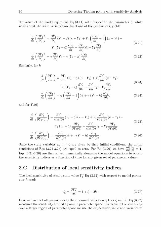
66 Detecting Tipping points with Sensitivity Analysis
derivative of the model equations Eq (3.11) with respect to the parameter ζ, whilenoting that the state variables are functions of the parameters, yields
d
dt
(∂Y1
∂ζ
)=∂Y1
∂ζ(Y1 − ζ) (κ− Y1) + Y1
(∂Y1
∂ζ− 1
)(κ− Y1)−
Y1 (Y1 − ζ)∂Y1
∂ζ− ∂Y1
∂ζY2 − Y1
∂Y2
∂ζ
(3.21)
d
dt
(∂Y2
∂ζ
)= γ
∂Y1
∂ζY2 + γ (Y1 − h)
∂Y2
∂ζ(3.22)
Similarly, for h
d
dt
(∂Y1
∂h
)=∂Y1
∂h(Y1 − ζ) (κ− Y1) + Y1
∂Y1
∂h(κ− Y1)−
Y1 (Y1 − ζ)∂Y1
∂h− ∂Y1
∂hY2 − Y1
∂Y2
∂h
(3.23)
d
dt
(∂Y2
∂h
)= γ
(∂Y1
∂h− 1
)Y2 + γ (Y1 − h)
∂Y2
∂h, (3.24)
and for Y2(0)
d
dt
(∂Y1
∂Y2(0)
)=
∂Y1
∂Y2(0)(Y1 − ζ) (κ− Y1) + Y1
∂Y1
∂Y2(0)(κ− Y1)−
Y1 (Y1 − ζ)∂Y1
∂Y2(0)− ∂Y1
∂Y2(0)Y2 − Y1
∂Y2
∂Y2(0)
(3.25)
d
dt
(∂Y2
∂Y2(0)
)= γ
∂Y1
∂Y2(0)Y2 + γ (Y1 − h)
∂Y2
∂Y2(0). (3.26)
Since the state variables at t = 0 are given by their initial conditions, the initialconditions of Eqs (3.21-3.25) are equal to zero. For Eq (3.26) we have ∂Y2(0)
∂Y2(0) = 1.Eqs (3.21-3.26) are then solved numerically alongside the model equations to obtainthe sensitivity indices as a function of time for any given set of parameter values.
3.C Distribution of local sensitivity indicesThe local sensitivity of steady state value Y ∗2 Eq (3.12) with respect to model param-eter h reads
s∗h =∂Y ∗2∂h
= 1 + ζ − 2h . (3.27)
Here we have set all parameters at their nominal values except for ζ and h. Eq (3.27)measures the sensitivity around a point in parameter space. To measure the sensitivityover a larger region of parameter space we use the expectation value and variance of

Chapter 3 67
Eq (3.27) over this region. For the stable steady state region (green) in Fig 3.2a wehave for the expectation value E(s∗h)
E(s∗h) =
∫ h=1
h=1/2
∫ ζ=2h−1
ζ=0
4s∗h dζ dh , (3.28)
where the factor 4 is a normalisation factor to ensure that the total probability isequal to one. This normalisation factor is equal to one divided by the area of thesurface over which we integrate. For the variance V (s∗h) we have
V (s∗h) =
∫ h=1
h=1/2
∫ ζ=2h−1
ζ=0
4(s∗h − E(s∗h))2 dζ dh . (3.29)
The local sensitivity of the steady state value Y ∗2 with respect to model parameter ζreads
s∗ζ =∂Y ∗2∂ζ
= h− κ . (3.30)
We have for the expectation value E(s∗ζ)
E(s∗ζ) =
∫ h=1
h=1/2
∫ ζ=2h−1
ζ=0
4s∗ζ dζ dh , (3.31)
and for the variance V (s∗ζ)
V (s∗ζ) =
∫ h=1
h=1/2
∫ ζ=2h−1
ζ=0
4(s∗ζ − E(s∗ζ))2 dζ dh . (3.32)
Instead of the local sensitivity index of Eq (3.27), the expectation value and variancemay be computed for the delsa sensitivity indices, by normalising the partial deriva-tive according to Eq (3.10). The calculation of the expectation value and the variancethen proceeds in the same way.
3.D Variance decomposition in Sobol’ methodThe variance decomposition Eq (3.4) follows from a decomposition of the model interms of the different model parameters (Sobol’ 2001, Saltelli et al. 2008). We writethe model as
Y = f(θ), (3.33)
where θ = (θ1, ..., θNp) ∈ INp and INp the Np−dimensional unit hypercube. Weassume uniform distributions between 0 and 1 for all parameters (θi ∼ U(0, 1)) anddecompose the model output as
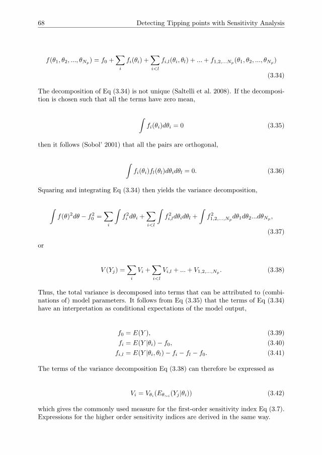
68 Detecting Tipping points with Sensitivity Analysis
f(θ1, θ2, ..., θNp) = f0 +
∑i
fi(θi) +∑i<l
fi,l(θi, θl) + ...+ f1,2,...Np(θ1, θ2, ..., θNp
)
(3.34)
The decomposition of Eq (3.34) is not unique (Saltelli et al. 2008). If the decomposi-tion is chosen such that all the terms have zero mean,
∫fi(θi)dθi = 0 (3.35)
then it follows (Sobol’ 2001) that all the pairs are orthogonal,
∫fi(θi)fl(θl)dθidθl = 0. (3.36)
Squaring and integrating Eq (3.34) then yields the variance decomposition,
∫f(θ)2dθ − f2
0 =∑i
∫f2i dθi +
∑i<l
∫f2i,ldθidθl +
∫f2
1,2,...,Npdθ1dθ2...dθNp
,
(3.37)
or
V (Yj) =∑i
Vi +∑i<l
Vi,l + ...+ V1,2,...,Np. (3.38)
Thus, the total variance is decomposed into terms that can be attributed to (combi-nations of) model parameters. It follows from Eq (3.35) that the terms of Eq (3.34)have an interpretation as conditional expectations of the model output,
f0 = E(Y ), (3.39)fi = E(Y |θi)− f0, (3.40)fi,l = E(Y |θi, θl)− fi − fl − f0. (3.41)
The terms of the variance decomposition Eq (3.38) can therefore be expressed as
Vi = Vθi(Eθ∼i(Yj |θi)) (3.42)
which gives the commonly used measure for the first-order sensitivity index Eq (3.7).Expressions for the higher order sensitivity indices are derived in the same way.
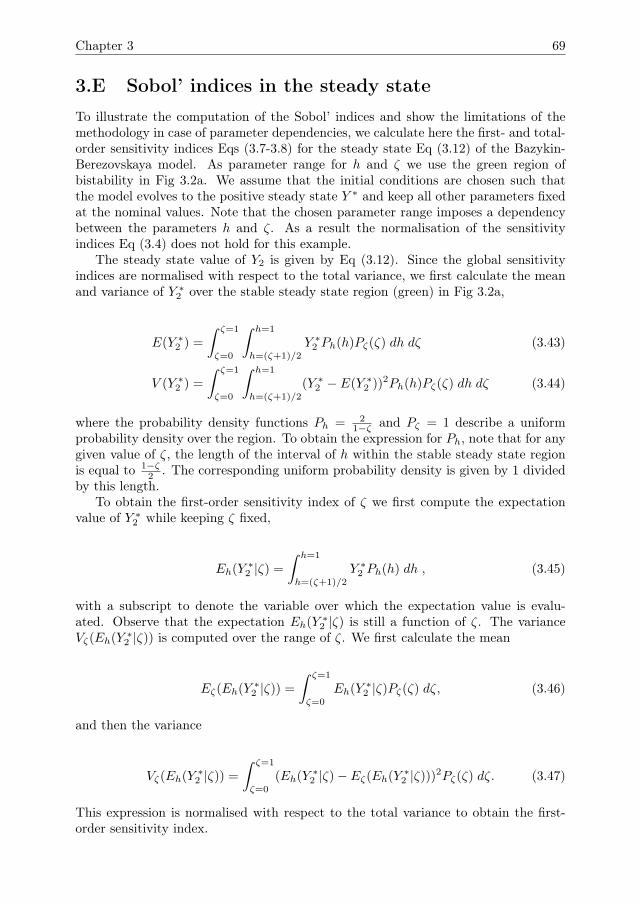
Chapter 3 69
3.E Sobol’ indices in the steady stateTo illustrate the computation of the Sobol’ indices and show the limitations of themethodology in case of parameter dependencies, we calculate here the first- and total-order sensitivity indices Eqs (3.7-3.8) for the steady state Eq (3.12) of the Bazykin-Berezovskaya model. As parameter range for h and ζ we use the green region ofbistability in Fig 3.2a. We assume that the initial conditions are chosen such thatthe model evolves to the positive steady state Y ∗ and keep all other parameters fixedat the nominal values. Note that the chosen parameter range imposes a dependencybetween the parameters h and ζ. As a result the normalisation of the sensitivityindices Eq (3.4) does not hold for this example.
The steady state value of Y2 is given by Eq (3.12). Since the global sensitivityindices are normalised with respect to the total variance, we first calculate the meanand variance of Y ∗2 over the stable steady state region (green) in Fig 3.2a,
E(Y ∗2 ) =
∫ ζ=1
ζ=0
∫ h=1
h=(ζ+1)/2
Y ∗2 Ph(h)Pζ(ζ) dh dζ (3.43)
V (Y ∗2 ) =
∫ ζ=1
ζ=0
∫ h=1
h=(ζ+1)/2
(Y ∗2 − E(Y ∗2 ))2Ph(h)Pζ(ζ) dh dζ (3.44)
where the probability density functions Ph = 21−ζ and Pζ = 1 describe a uniform
probability density over the region. To obtain the expression for Ph, note that for anygiven value of ζ, the length of the interval of h within the stable steady state regionis equal to 1−ζ
2 . The corresponding uniform probability density is given by 1 dividedby this length.
To obtain the first-order sensitivity index of ζ we first compute the expectationvalue of Y ∗2 while keeping ζ fixed,
Eh(Y ∗2 |ζ) =
∫ h=1
h=(ζ+1)/2
Y ∗2 Ph(h) dh , (3.45)
with a subscript to denote the variable over which the expectation value is evalu-ated. Observe that the expectation Eh(Y ∗2 |ζ) is still a function of ζ. The varianceVζ(Eh(Y ∗2 |ζ)) is computed over the range of ζ. We first calculate the mean
Eζ(Eh(Y ∗2 |ζ)) =
∫ ζ=1
ζ=0
Eh(Y ∗2 |ζ)Pζ(ζ) dζ, (3.46)
and then the variance
Vζ(Eh(Y ∗2 |ζ)) =
∫ ζ=1
ζ=0
(Eh(Y ∗2 |ζ)− Eζ(Eh(Y ∗2 |ζ)))2Pζ(ζ) dζ. (3.47)
This expression is normalised with respect to the total variance to obtain the first-order sensitivity index.
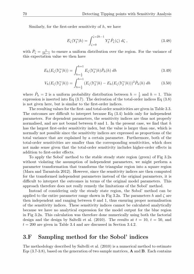
70 Detecting Tipping points with Sensitivity Analysis
Similarly, for the first-order sensitivity of h, we have
Eζ(Y∗2 |h) =
∫ ζ=2h−1
ζ=0
Y ∗2 P̂ζ(ζ) dζ , (3.48)
with P̂ζ = 12h−1 to ensure a uniform distribution over the region. For the variance of
this expectation value we then have
Eh(Eζ(Y∗2 |h)) =
∫ h=1
h= 12
Eζ(Y∗2 |h)P̂h(h) dh (3.49)
Vh(Eζ(Y∗2 |h)) =
∫ h=1
h= 12
(Eζ(Y∗2 |h)− Eh(Eζ(Y
∗2 |h)))2P̂h(h) dh (3.50)
where P̂h = 2 is a uniform probability distribution between h = 12 and h = 1. This
expression is inserted into Eq (3.7). The derivation of the total-order indices Eq (3.8)is not given here, but is similar to the first-order indices.
The resulting values for the first- and total-order sensitivities are given in Table 3.3.The outcomes are difficult to interpret because Eq (3.4) holds only for independentparameters. For dependent parameters, the sensitivity indices are thus not properlynormalised, and are not bound between 0 and 1. In the present case, we find that hhas the largest first-order sensitivity index, but the value is larger than one, which isnormally not possible since the sensitivity indices are expressed as proportions of thetotal variance that are explained by a certain parameter. Furthermore, both of thetotal-order sensitivities are smaller than the corresponding sensitivities, which doesnot make sense given that the total-order sensitivity includes higher-order effects inaddition to first-order effects.
To apply the Sobol’ method to the stable steady state region (green) of Fig 3.2awithout violating the assumption of independent parameters, we might perform aparameter transformation that transforms the triangular region into a square region(Mara and Tarantola 2012). However, since the sensitivity indices are then computedfor the transformed independent parameters instead of the original parameters, it isdifficult to interpret the outcomes in terms of the original model parameters. Thisapproach therefore does not really remedy the limitations of the Sobol’ method.
Instead of considering only the steady state region, the Sobol’ method can beapplied to the entire parameter range shown in Fig 3.2a. The parameters h and ζ arethen independent and ranging between 0 and 1, thus ensuring proper normalisationof the sensitivity indices. These sensitivity indices cannot be calculated analyticallybecause we have no analytical expression for the model output for the blue regionin Fig 3.2a. This calculation was therefore done numerically using both the factorialdesign and the design by Saltelli et al. (2010). The results at t = 10, t = 50, andt = 200 are given in Table 3.4 and are discussed in Section 3.4.2.
3.F Sampling method for the Sobol’ indicesThe methodology described by Saltelli et al. (2010) is a numerical method to estimateEqs (3.7-3.8), based on the generation of two sample matrices, A and B. Each contains
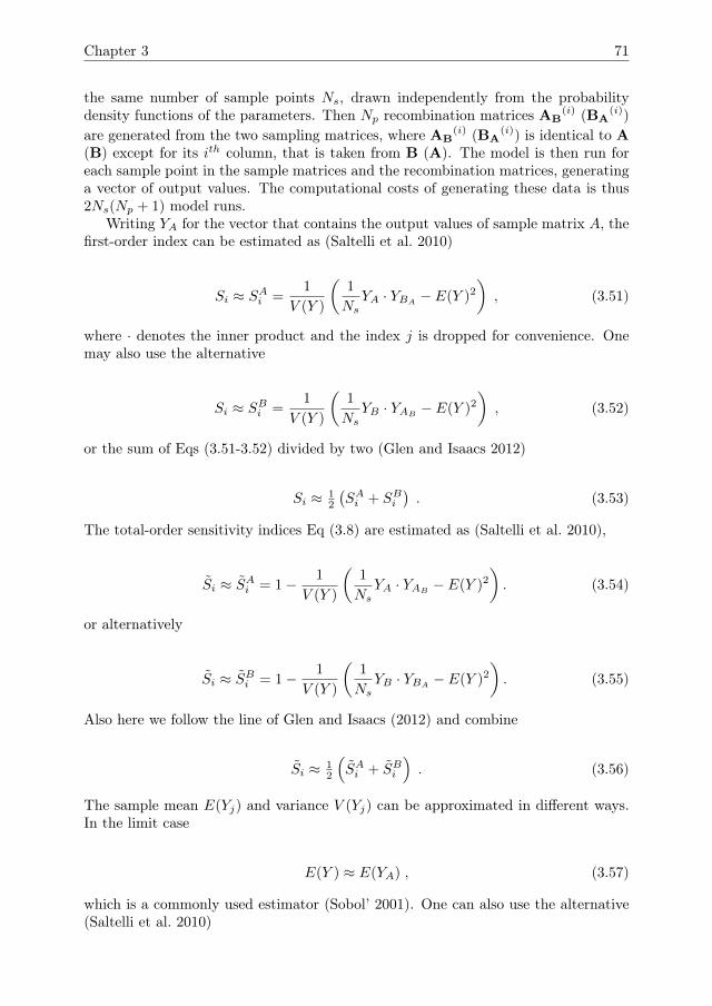
Chapter 3 71
the same number of sample points Ns, drawn independently from the probabilitydensity functions of the parameters. Then Np recombination matrices AB
(i) (BA(i))
are generated from the two sampling matrices, where AB(i) (BA
(i)) is identical to A(B) except for its ith column, that is taken from B (A). The model is then run foreach sample point in the sample matrices and the recombination matrices, generatinga vector of output values. The computational costs of generating these data is thus2Ns(Np + 1) model runs.
Writing YA for the vector that contains the output values of sample matrix A, thefirst-order index can be estimated as (Saltelli et al. 2010)
Si ≈ SAi =1
V (Y )
(1
NsYA · YBA
− E(Y )2
), (3.51)
where · denotes the inner product and the index j is dropped for convenience. Onemay also use the alternative
Si ≈ SBi =1
V (Y )
(1
NsYB · YAB
− E(Y )2
), (3.52)
or the sum of Eqs (3.51-3.52) divided by two (Glen and Isaacs 2012)
Si ≈ 12
(SAi + SBi
). (3.53)
The total-order sensitivity indices Eq (3.8) are estimated as (Saltelli et al. 2010),
S̃i ≈ S̃Ai = 1− 1
V (Y )
(1
NsYA · YAB
− E(Y )2
). (3.54)
or alternatively
S̃i ≈ S̃Bi = 1− 1
V (Y )
(1
NsYB · YBA
− E(Y )2
). (3.55)
Also here we follow the line of Glen and Isaacs (2012) and combine
S̃i ≈ 12
(S̃Ai + S̃Bi
). (3.56)
The sample mean E(Yj) and variance V (Yj) can be approximated in different ways.In the limit case
E(Y ) ≈ E(YA) , (3.57)
which is a commonly used estimator (Sobol’ 2001). One can also use the alternative(Saltelli et al. 2010)
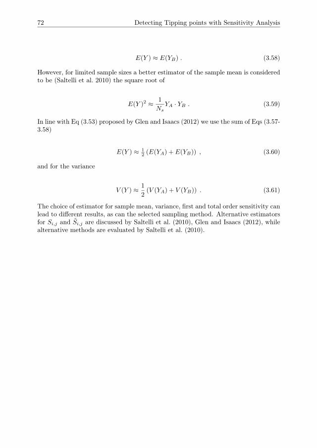
72 Detecting Tipping points with Sensitivity Analysis
E(Y ) ≈ E(YB) . (3.58)
However, for limited sample sizes a better estimator of the sample mean is consideredto be (Saltelli et al. 2010) the square root of
E(Y )2 ≈ 1
NsYA · YB . (3.59)
In line with Eq (3.53) proposed by Glen and Isaacs (2012) we use the sum of Eqs (3.57-3.58)
E(Y ) ≈ 12 (E(YA) + E(YB)) , (3.60)
and for the variance
V (Y ) ≈ 1
2(V (YA) + V (YB)) . (3.61)
The choice of estimator for sample mean, variance, first and total order sensitivity canlead to different results, as can the selected sampling method. Alternative estimatorsfor Si,j and S̃i,j are discussed by Saltelli et al. (2010), Glen and Isaacs (2012), whilealternative methods are evaluated by Saltelli et al. (2010).
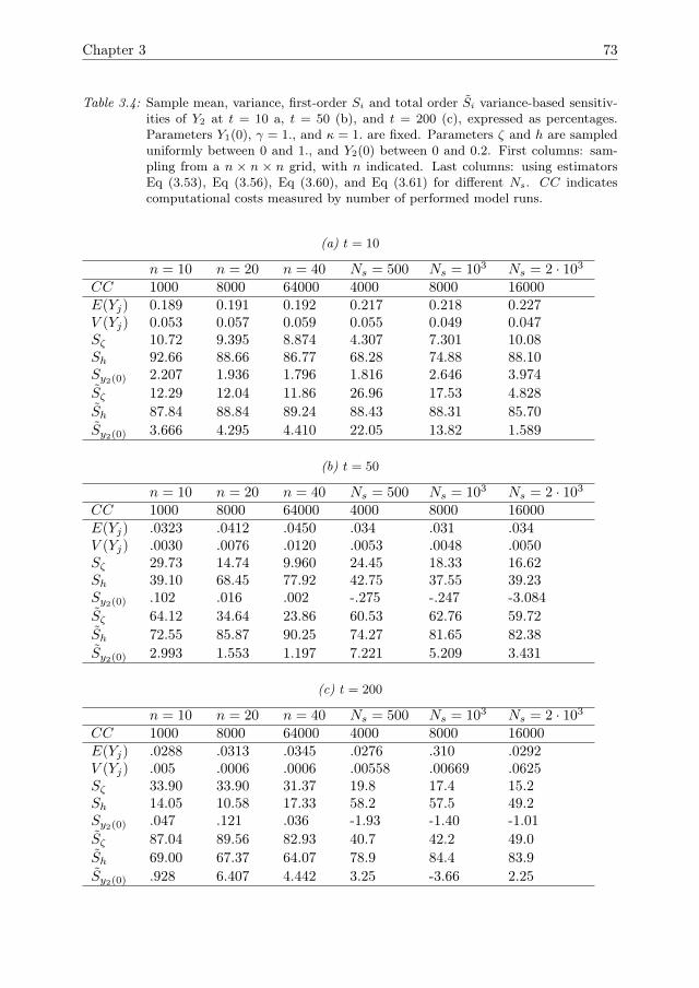
Chapter 3 73
Table 3.4: Sample mean, variance, first-order Si and total order S̃i variance-based sensitiv-ities of Y2 at t = 10 a, t = 50 (b), and t = 200 (c), expressed as percentages.Parameters Y1(0), γ = 1., and κ = 1. are fixed. Parameters ζ and h are sampleduniformly between 0 and 1., and Y2(0) between 0 and 0.2. First columns: sam-pling from a n × n × n grid, with n indicated. Last columns: using estimatorsEq (3.53), Eq (3.56), Eq (3.60), and Eq (3.61) for different Ns. CC indicatescomputational costs measured by number of performed model runs.
(a) t = 10
n = 10 n = 20 n = 40 Ns = 500 Ns = 103 Ns = 2 · 103
CC 1000 8000 64000 4000 8000 16000E(Yj) 0.189 0.191 0.192 0.217 0.218 0.227V (Yj) 0.053 0.057 0.059 0.055 0.049 0.047Sζ 10.72 9.395 8.874 4.307 7.301 10.08Sh 92.66 88.66 86.77 68.28 74.88 88.10Sy2(0) 2.207 1.936 1.796 1.816 2.646 3.974S̃ζ 12.29 12.04 11.86 26.96 17.53 4.828S̃h 87.84 88.84 89.24 88.43 88.31 85.70S̃y2(0) 3.666 4.295 4.410 22.05 13.82 1.589
(b) t = 50
n = 10 n = 20 n = 40 Ns = 500 Ns = 103 Ns = 2 · 103
CC 1000 8000 64000 4000 8000 16000E(Yj) .0323 .0412 .0450 .034 .031 .034V (Yj) .0030 .0076 .0120 .0053 .0048 .0050Sζ 29.73 14.74 9.960 24.45 18.33 16.62Sh 39.10 68.45 77.92 42.75 37.55 39.23Sy2(0) .102 .016 .002 -.275 -.247 -3.084S̃ζ 64.12 34.64 23.86 60.53 62.76 59.72S̃h 72.55 85.87 90.25 74.27 81.65 82.38S̃y2(0) 2.993 1.553 1.197 7.221 5.209 3.431
(c) t = 200
n = 10 n = 20 n = 40 Ns = 500 Ns = 103 Ns = 2 · 103
CC 1000 8000 64000 4000 8000 16000E(Yj) .0288 .0313 .0345 .0276 .310 .0292V (Yj) .005 .0006 .0006 .00558 .00669 .0625Sζ 33.90 33.90 31.37 19.8 17.4 15.2Sh 14.05 10.58 17.33 58.2 57.5 49.2Sy2(0) .047 .121 .036 -1.93 -1.40 -1.01S̃ζ 87.04 89.56 82.93 40.7 42.2 49.0S̃h 69.00 67.37 64.07 78.9 84.4 83.9S̃y2(0) .928 6.407 4.442 3.25 -3.66 2.25

Chapter 4
Which sensitivity analysismethod should I use for myAgent-based Model?
G.A. ten Broeke, G.A.K. van Voorn, A. Ligtenberg.Journal of Artificial Societies and Social Simulation, 19(1).
76 Which sensitivity analysis method should I use for my ABM?
Existing methodologies of sensitivity analysis may be insufficient for a proper analy-sis of Agent-based Models (ABMs). Most ABMs consist of multiple levels, containvarious nonlinear interactions, and display emergent behaviour. This limits the in-formation content that follows from the classical sensitivity analysis methodologiesthat link model output to model input. In this paper we evaluate the performanceof three well-known methodologies for sensitivity analysis of ABMs. The threemethodologies are OFAT (one-factor-at-a-time), and proportional assigning of out-put variance by means of model fitting and by means of Sobol’ decomposition. Themethodologies are applied to an ABM case study of limited complexity consistingof free-roaming and procreating agents that make harvest decisions with regard toa diffusing renewable resource. We find that each methodology has its own meritsand yields useful information, yet none of them provide a complete picture of modelbehaviour. We recommend OFAT as the starting point for sensitivity analysis ofan ABM, for its use in uncovering the mechanisms and patterns that the ABMproduces.
4.1 Introduction
During the last decade Agent Based Models (ABMs) have become a standard tech-nique in the toolbox of scholars interested in simulating and understanding complexadaptive systems such as land use systems (Parker et al. 2003, Bousquet and Le Page2004, Matthews et al. 2007). Still missing are solid methods to explore the behaviourof an ABM and assess its relation with the empirical world (Crooks et al. 2008, Fi-latova et al. 2013). For ABMs to be useful as tools to learn about and understandcomplex adaptive systems it is essential to know the effects of different configurationsof system components on global and emergent outcomes. These insights are especiallycrucial when one is interested in studying the conditions under which systems can be-come critical, i.e. when resilience and when tipping points can occur, for instance,when one wants to obtain early warning signals.
In order to explore the behaviour of models sensitivity analysis is a commonlyused tool, at least in the field of traditional modelling. There exists a plethora ofstandardized methodologies for performing sensitivity analysis (Saltelli et al. 2004b,2008, Hamby 1994, Cariboni et al. 2007, Thiele et al. 2014). However it is unclearto what extent these methodologies are suitable for the type of systems commonlyrepresented by ABMs. It is important to observe though that all sensitivity analysismethodologies have a statistical underpinning. It is because of the statistical approachthere is no mechanistic focus, and results obtained via sensitivity analysis alwaysrequire an interpretation by model users in the context of the model application.
ABMs are characterized by several properties that make the application of anystatistical approach, and thus most standard sensitivity analysis methods, a nontrivialmatter. These properties are (Windrum et al. 2007, Gilbert 2008, Macal and North2010)
• The existence of multiple levels. There is at least a micro-level consisting of in-dividual and autonomous agents, and a macro-level environment that influences
Chapter 4 77
and is influenced by the agents. This implies there are also at least two distinctsteps going from input to output;
• The existence of many and often nonlinear interactions. This suggests thatrelations between input and output may be nonlinear as well;
• The existence of emergent properties, i.e. patterns that are not predicted apriori based on the individual rules describing either the agent or the envi-ronment. Such patterns are for example path dependencies, adaptation, andtipping points. This also suggests that the relations between input and outputmay be nonlinear, and, additionally, may change over time.
It is for this reason that a straightforward application of classical methodologies forsensitivity analysis to ABMs will not always yield sufficient information required bythe model user for model evaluation. The main complicating factor is that for most,if not all, complex adaptive systems the interactions and relations between systemcomponents are self-organizing processes. Relations between global system states(i.e., the outputs) and the states of the individual system components (i.e., the inputs)are not pre-defined like in traditional linear models. Different system states mightbe possible under similar parameter regimes, while completely different parameterregimes might yield similar system behaviour. This means that a standard sensitivityanalysis performed on an ABM has only limited explanatory power. Developingtargeted methods of sensitivity analysis has therefore rightly been identified as a keychallenge for Agent-based Modelling (Crooks et al. 2008, Filatova et al. 2013, Thieleet al. 2014). In turn, the analysis, calibration, and validation of ABMs also remainpivotal issues (Brown et al. 2005, Fagiolo et al. 2007, Windrum et al. 2007, Crookset al. 2008, Filatova et al. 2013).
In this paper we explore the potential of three well-known methodologies for sensi-tivity analysis to obtain information that is useful for a) assessing the implementationof an ABM and b) understanding the behaviour of the represented system. The threemethodologies are described in Section 4.3. To have a measure of quantification ofthe potential of the elected methodologies, three goals have been selected which aretypical for ABM applications. These goals are explained in 4.2. In 4.4 we present acase study model to apply the sensitivity analysis methodologies to. The details ofthe model are given in 4.A in ODD format. The choice of the case study is justifiedby the relatively low complexity of the model, which limits computational costs, whilethe model contains all the essential ingredients of an ABM. 4.5 gives an overview ofthe main results. 4.6 finalizes with the discussion.
4.2 Selected goals for performing sensitivity analysis
We have selected three application goals for sensitivity analysis which are commonfor ABM research. These are
• To gain insight in how patterns and emergent properties are generated in theABM;
• To examine the robustness of emergent properties;
78 Which sensitivity analysis method should I use for my ABM?
• To quantify the variability in ABM outcomes resulting from model parameters.
To better understand dynamics and emergent patterns found in the real-world systemsthat are described by ABMs it is crucial to first understand how they are generated inthe model. Given the complexity of many ABMs, understanding the model dynamicsis typically not a straightforward task. Sensitivity analysis can help in this taskbecause the effects of parameter changes on the model outcomes contain clues aboutthe model dynamics underlying these outcomes (Ligmann-Zielinska et al. 2014). Forexample, revealing whether these effects are linear, non-linear, or push the systeminto an entirely different state by causing a tipping point yields valuable informationon how a parameter affects the dynamics of the system.
A second motivation for performing sensitivity analysis is to examine the robust-ness of the model outcomes with respect to changes of the parameter values (Leamer1983, 2010, Axtell 1999). A range of model parameter values corresponds to a rangeof assumptions that leads to certain inferences (i.e. model outcomes). For these in-ferences to be credible, however, they should not depend on a narrow and uncertainset of assumptions. It is therefore important to show that the inferences are robustto parameter changes. This is particularly relevant if the model attempts to explaina phenomenon that occurs under a wide range of circumstances in reality. For ex-ample, the well-known Schelling model (Schelling 1971) examines the emergence ofpatterns of ethnic segregation. The model shows that patterns of segregation emergefrom a few simple assumptions on the movement of agents in a spatial environment.Furthermore, this emergence is robust to changes in the parameter values and move-ment rules of the agents (Gilbert 2002). This robustness adds to the credibility of themodel, given the observation that segregation in reality occurs in different places andunder various circumstances. A third and more traditional use of sensitivity analysisis to quantify the uncertainty of the model outcomes that is caused by parameteruncertainties (Hamby 1994, Saltelli et al. 2008). There are various sources that con-tribute to uncertainty of the model outcomes. One of these sources is uncertaintyin the parameter set. We typically assign values to the model parameters based onmeasurements or expert judgements, but there is uncertainty in these values. Theuncertainty of the parameter set causes uncertainty in the model outcomes. Sensi-tivity analysis quantifies this output variability and decomposes it into terms thatare attributed to different parameters. This allows the user to rank the input uncer-tainties in terms of their contribution to output uncertainty. This ranking can forexample be used to decrease the output uncertainty by decreasing the uncertainty ofthe parameter set.
4.3 Selected methodologies for sensitivity analysisMany methodologies have been developed to perform sensitivity analysis (for anoverview see for instance (Saltelli et al. 2004b, 2008, Cariboni et al. 2007)). Herewe have selected three methodologies. These are
• Sensitivities based on one-factor-at-a-time (OFAT);
• Sensitivities based on model-free output variance decomposition;
• Sensitivities based on model-based output variance decomposition.
Chapter 4 79
These methodologies have been selected because they are commonly available in sta-tistical packages (e.g. Thiele et al. (2014)), while they have proven to be very popularsince they can be applied rather straightforwardly with limited statistical and com-putational efforts. We discuss the three methodologies in more detail below.
4.3.1 One-factor-at-a-time (OFAT)
OFAT sensitivity analysis essentially consists of selecting a base parameter setting(nominal set) and varying one parameter at a time while keeping all other parametersfixed (hence it is referred to as a local method). An important use of OFAT is to revealthe form of the relationship between the varied parameter and the output, given thatall other parameters have their nominal values. For example, it shows whether theresponse is linear or nonlinear, or whether there are tipping points where the outputresponds drastically to a small parameter change. By showing these relationships,OFAT can yield understanding of model mechanisms. For this purpose, we vary eachparameter over a number of points within a wide range and plot the resulting output.
Note that One-at-a-time (OAT) is traditionally used to estimate sensitivity mea-sures in the form of partial derivatives of the model outcomes with respect to inputparameters (e.g. Cariboni et al. (2007)). This estimation is based on the effect ofsmall deviations from the nominal parameter values on the model outcomes. OFATdiffers from OAT in that we examine the model response over a wide range for eachparameter. The slope of the output graph at some parameter value roughly estimatesthe partial derivative at that point. A more accurate estimate would require a smallerstep size in the parameter values and a large number of replicate runs to account forstochastic effects. However, such an estimate does not directly contribute towards ouraim of showing the form of the relationship between the parameter and the output.We therefore do not explicitly compute these partial derivatives.
4.3.2 Global sensitivity analysis
Global sensitivity analysis (Saltelli et al. 2008) aims to ascertain interaction effectsby sampling the model output over a wide range of parameter values. Many samples(i.e. specific parameter settings, usually determined randomly) are drawn from theparameter space, and the corresponding model outcomes are combined in a statisticalmeasure, namely the variance of the output of the model. The sensitivity to a param-eter is then measured as the proportion of the model variance that can be explainedby changes in that parameter. Since the total model variance is used to normalise thesensitivities, the sensitivities of different parameters can be compared directly. Thereare two common ways to decompose the output variance:
• By using a regression model to fit the model output to model parameters, in asimilar fashion as regular regression is done, for instance by means of ordinaryleast squares (OLS);
• By using the decomposition of Sobol’ (Sobol’ 2001), which does not involve theuse of a regression model, but estimates the contributions of different combina-tions of parameters to the output variance while making the assumption thatall parameters are independent.
80 Which sensitivity analysis method should I use for my ABM?
Based on the decomposition, sensitivity measures are defined that express theexplained variance for different combinations of parameters. The two most commonlyreported measures are the first and total-order indices (Saltelli et al. 2008). The first-order index of a parameter is defined as the reduction of the model variance thatwould occur, on average, if the parameter became exactly known. The total-orderindex is defined as the proportion of the variance that would remain, on average, whenall other parameters are exactly known. If the input distributions of the parametersare independent, the difference between the first- and total-order index of a parametermeasures the explained variance by all of the interactions with other parameters.
Regression-based
Regression-based methods decompose the variance of the ABM outcomes by fittinga regression function of the input parameters to these outcomes (e.g. Downing et al.(1985)). An advantage of such an approach is that the output of the complex ABMis condensed into descriptive relationships, which can be validated against data usingcommon statistical measures (such as R2) and which help thinking about influentialprocesses.
However, these relationships are good descriptions of the ABM output only if theregression function is a good fit to the output. If the fit does not explain most ofthe variance (e.g. > 90%) then other regression functions may be tried until a betterfit is obtained. Finding a good regression function is thus an iterative process and isa main challenge for regression-based sensitivity analysis, especially for models withcomplex relations between the input and output.
Various regression methods are available (Draper and Smith 2014). Here we useordinary least squares (OLS) regression because this method is the most commonlyused. It optimises the R2 measure for linear regression,
R2 = 1−∑(
yj − yrj)2∑
(yj − yav)2 . (4.1)
The summation runs over a number of sample points with different parameter values,yj is the vector of model outcomes, yrj is vector of predicted outcomes by the regressionmodel and yav is the mean of the model outcomes. The value of R2 is interpreted asthe explained variance by the regression model. Thus, OLS straightforwardly yields avariance decomposition. The first-order sensitivity index of parameter i is computedas the value of R2 when excluding that parameter from the fit,
Sr,i = 1−∑(
yj − yrj)2∑
(yj − yav)2 . (4.2)
where yrj is the predicted outcome by the regression function excluding parameteri. Similarly, the total-order sensitivity index is computed as the explained variancewhen keeping parameter i, but leaving out all other parameters,
Stot,r,i = 1−∑(
yj − yrj)2∑
(yj − yav)2 . (4.3)
where yr′
j is the predicted outcome by the regression function including only parameteri.
Chapter 4 81
Sobol’ method
In contrast to regression-based methods, the Sobol’ method is model-free, i.e. nofitting functions are used to decompose the output variance (Saltelli et al. 2008). Themethod is based on a decomposition of the model variance V (y) that holds if theinput parameters are independent,
V (Y ) =∑i
Vi +∑i,j
Vi,j + ...+ Vi,j,...,m (4.4)
where the partial variance is defined as
Vi = Vxi(Ex i(y|x)) (4.5)
with x i denoting all parameters except for xi. The expectation value of the modeloutput is computed while keeping the parameter fixed and varying all other parame-ters. The variance of this expectation value is then computed over the possible valuesof xi. Thus, if Vi is large, the expected model outcome strongly varies dependingon xi, indicating the parameter to be sensitive. Sensitivity indices are defined byconsidering the partial variance relative to the total variance,
Ss,i =ViV (y)
. (4.6)
Higher-order sensitivity indices are defined by computing the partial variance over twoor more parameters instead of a single parameter. The total and partial variances areusually estimated from a Monte Carlo sample.
The estimated sensitivity indices by themselves are not meaningful unless we knowthe accuracy of the estimate. We therefore use a bootstrap method (Archer et al.1997) to assess this accuracy. We create a number of bootstrap samples by drawingindependent points from the original Monte Carlo sample. Each bootstrap sampleis equal in size to the original Monte Carlo sample. We then compute the first- andtotal-order sensitivity indices based on each bootstrap sample. The distribution ofthese sensitivity indices estimates the accuracy of the sensitivity indices based on theoriginal sample. If the bootstrap sensitivity indices are normally distributed, thenwe can construct a confidence interval based on the standard error of the bootstrapsensitivity indices.
4.4 Model test case: agents harvesting a diffusingrenewable resource
The case study concerns an ABM coded in NetLogo (Wilensky 1999) that describesindividual agents in a spatially explicit environment. The model flowchart for a singletime-step is shown in Fig 4.1. The environment is updated by growth and diffusion ofa renewable resource (‘food’). The agents observe their local surroundings and decidewhether to harvest or not and to move or not, based on their own (decreasing) internalenergy state that needs to be replenished, as well as the state of the outside world,which includes the local presence of resource (‘food availability’) and other agents
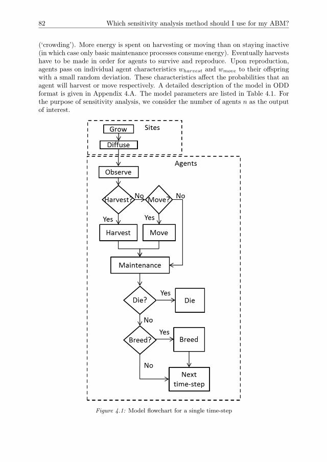
82 Which sensitivity analysis method should I use for my ABM?
(‘crowding’). More energy is spent on harvesting or moving than on staying inactive(in which case only basic maintenance processes consume energy). Eventually harvestshave to be made in order for agents to survive and reproduce. Upon reproduction,agents pass on individual agent characteristics wharvest and wmove to their offspringwith a small random deviation. These characteristics affect the probabilities that anagent will harvest or move respectively. A detailed description of the model in ODDformat is given in Appendix 4.A. The model parameters are listed in Table 4.1. Forthe purpose of sensitivity analysis, we consider the number of agents n as the outputof interest.
Figure 4.1: Model flowchart for a single time-step

Chapter 4 83
Tab
le4.
1:Mod
elpa
rametersan
drang
eforsensitivityan
alysis
Symbo
lDescription
Units/R
ange
Nom
inal
value
Ran
gefor
OFAT
Ran
geforglob
alSA
cHarvest
efficiency
Jkg−
10.9
0.1–1
0–1
DDiffusioncoeffi
cient
km2da
y−1
0.1
0–0.25
0–0.25
Eb
Birth
energy
J6.5
1–10
1–10
Eh
Harvest
cost
J0.1
0–0.5
0–0.5
Em
Costof
energy
maintenan
ceJ
0.1
0.05
–0.5
0–0.5
Emove
Movecost
J0.5
0–2
0–2
KResou
rcecarrying
capa
city
kg2
0.5–5
0–5
n0
Initialn
umbe
rof
agents
0,1,
2,...
100
0–1000
0–400
RResou
rcegrow
thrate
s−1
0.1
0–0.5
0–0.5
R0
Initialr
esou
rcelevel
0-1
(propo
rtion
ofK)
10–1
0–1
Rmax
Max
imum
harvestpe
rtime-step
kg0.5
0.2–2
0.2–2
Runc
Uncertainty
ofresource
estimations
kg0.1
0–1
0–1
v bAgent
birthcoeffi
cient
J−1
100–20
0–20
v dAgent
mortalitycoeffi
cient
J−1
100–20
0–20
zVariation
inoff
spring
traits
[0,→〉
0.2
0–0.5
0–0.5
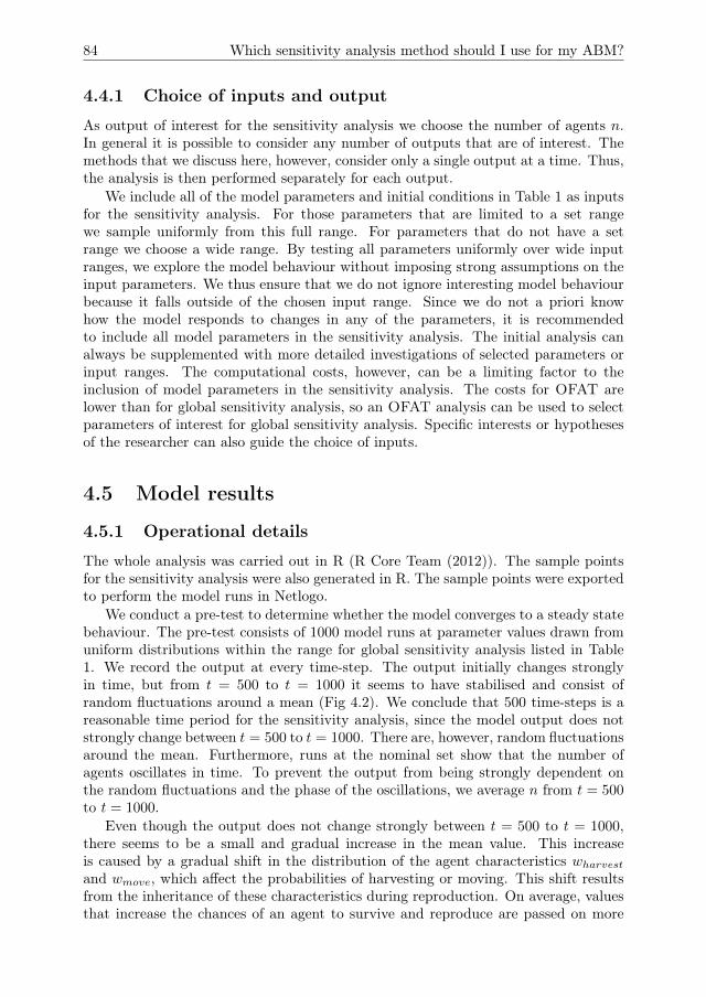
84 Which sensitivity analysis method should I use for my ABM?
4.4.1 Choice of inputs and output
As output of interest for the sensitivity analysis we choose the number of agents n.In general it is possible to consider any number of outputs that are of interest. Themethods that we discuss here, however, consider only a single output at a time. Thus,the analysis is then performed separately for each output.
We include all of the model parameters and initial conditions in Table 1 as inputsfor the sensitivity analysis. For those parameters that are limited to a set rangewe sample uniformly from this full range. For parameters that do not have a setrange we choose a wide range. By testing all parameters uniformly over wide inputranges, we explore the model behaviour without imposing strong assumptions on theinput parameters. We thus ensure that we do not ignore interesting model behaviourbecause it falls outside of the chosen input range. Since we do not a priori knowhow the model responds to changes in any of the parameters, it is recommendedto include all model parameters in the sensitivity analysis. The initial analysis canalways be supplemented with more detailed investigations of selected parameters orinput ranges. The computational costs, however, can be a limiting factor to theinclusion of model parameters in the sensitivity analysis. The costs for OFAT arelower than for global sensitivity analysis, so an OFAT analysis can be used to selectparameters of interest for global sensitivity analysis. Specific interests or hypothesesof the researcher can also guide the choice of inputs.
4.5 Model results
4.5.1 Operational details
The whole analysis was carried out in R (R Core Team (2012)). The sample pointsfor the sensitivity analysis were also generated in R. The sample points were exportedto perform the model runs in Netlogo.
We conduct a pre-test to determine whether the model converges to a steady statebehaviour. The pre-test consists of 1000 model runs at parameter values drawn fromuniform distributions within the range for global sensitivity analysis listed in Table1. We record the output at every time-step. The output initially changes stronglyin time, but from t = 500 to t = 1000 it seems to have stabilised and consist ofrandom fluctuations around a mean (Fig 4.2). We conclude that 500 time-steps is areasonable time period for the sensitivity analysis, since the model output does notstrongly change between t = 500 to t = 1000. There are, however, random fluctuationsaround the mean. Furthermore, runs at the nominal set show that the number ofagents oscillates in time. To prevent the output from being strongly dependent onthe random fluctuations and the phase of the oscillations, we average n from t = 500to t = 1000.
Even though the output does not change strongly between t = 500 to t = 1000,there seems to be a small and gradual increase in the mean value. This increaseis caused by a gradual shift in the distribution of the agent characteristics wharvestand wmove, which affect the probabilities of harvesting or moving. This shift resultsfrom the inheritance of these characteristics during reproduction. On average, valuesthat increase the chances of an agent to survive and reproduce are passed on more
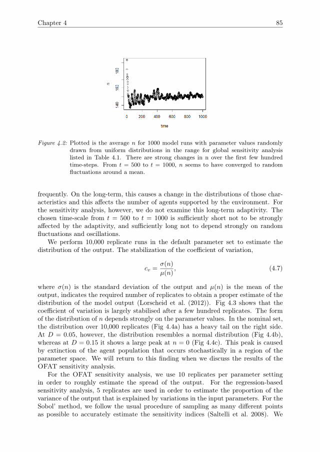
Chapter 4 85
Figure 4.2: Plotted is the average n for 1000 model runs with parameter values randomlydrawn from uniform distributions in the range for global sensitivity analysislisted in Table 4.1. There are strong changes in n over the first few hundredtime-steps. From t = 500 to t = 1000, n seems to have converged to randomfluctuations around a mean.
frequently. On the long-term, this causes a change in the distributions of those char-acteristics and this affects the number of agents supported by the environment. Forthe sensitivity analysis, however, we do not examine this long-term adaptivity. Thechosen time-scale from t = 500 to t = 1000 is sufficiently short not to be stronglyaffected by the adaptivity, and sufficiently long not to depend strongly on randomfluctuations and oscillations.
We perform 10,000 replicate runs in the default parameter set to estimate thedistribution of the output. The stabilization of the coefficient of variation,
cv =σ(n)
µ(n), (4.7)
where σ(n) is the standard deviation of the output and µ(n) is the mean of theoutput, indicates the required number of replicates to obtain a proper estimate of thedistribution of the model output (Lorscheid et al. (2012)). Fig 4.3 shows that thecoefficient of variation is largely stabilised after a few hundred replicates. The formof the distribution of n depends strongly on the parameter values. In the nominal set,the distribution over 10,000 replicates (Fig 4.4a) has a heavy tail on the right side.At D = 0.05, however, the distribution resembles a normal distribution (Fig 4.4b),whereas at D = 0.15 it shows a large peak at n = 0 (Fig 4.4c). This peak is causedby extinction of the agent population that occurs stochastically in a region of theparameter space. We will return to this finding when we discuss the results of theOFAT sensitivity analysis.
For the OFAT sensitivity analysis, we use 10 replicates per parameter settingin order to roughly estimate the spread of the output. For the regression-basedsensitivity analysis, 5 replicates are used in order to estimate the proportion of thevariance of the output that is explained by variations in the input parameters. For theSobol’ method, we follow the usual procedure of sampling as many different pointsas possible to accurately estimate the sensitivity indices (Saltelli et al. 2008). We
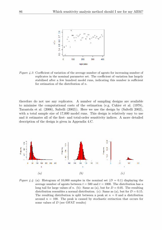
86 Which sensitivity analysis method should I use for my ABM?
Figure 4.3: Coefficient of variation of the average number of agents for increasing number ofreplicates in the nominal parameter set. The coefficient of variation has largelystabilised after a few hundred model runs, indicating this number is sufficientfor estimation of the distribution of n.
therefore do not use any replicates. A number of sampling designs are availableto minimise the computational costs of the estimation (e.g. Cukier et al. (1978),Tarantola et al. (2006), Saltelli (2002)). Here we use the design by (Saltelli 2002),with a total sample size of 17,000 model runs. This design is relatively easy to useand it estimates all of the first- and total-order sensitivity indices. A more detaileddescription of the design is given in Appendix 4.C.
(a) (b) (c)
Figure 4.4: (a): Histogram of 10,000 samples in the nominal set (D = 0.1) displaying theaverage number of agents between t = 500 and t = 1000. The distribution has along tail for large values of n. (b): Same as (a), but for D = 0.05. The resultingdistribution resembles a normal distribution. (c): Same as (a), but for D = 0.15.The resulting distribution is split between a peak at n = 0 and a distributionaround n = 100. The peak is caused by stochastic extinction that occurs forsome values of D (see OFAT results)
Chapter 4 87
4.5.2 One-factor-at-a-time sensitivity analysis
We perform OFAT sensitivity analysis for all of the model parameters. The defaultvalues and ranges of variation of all parameters are listed in Table 4.1. We runthe model for the extreme values of this range and 9 equidistant points in between.The resulting graph for the diffusivity (Fig 4.5) shows two tipping points where thenumber of agents goes to zero. When D = 0, sites without resource cannot bereplenished through diffusion from neighbouring sites, eventually leading to collapseof the system. Inspection of the time-series of a number of model runs reveals thatthe number of agents oscillates with increasing amplitude for increasing values of D.Between D = 0.10 and D = 0.15 this amplitude becomes so large that n crosses zero,causing the system to collapse. Because the model is stochastic, this collapse occursin some but not all of the replicates. Tests with longer simulation times than 1000time-steps show that between D = 0.10 and D = 0.15 extinction occurs mostly duringthe first 1000 time-steps. If extinction does not occur during this initial period, thenn remains positive on the long term. The model thus has multiple equilibria for theseparameter values. For D ≤ 0.175 the population always goes to extinction, but forD = 0.175 it sometimes takes more than 1000 time-steps before this equilibrium isreached. One of the model runs in Fig 4.5 therefore still has a positive populationafter 1000 time-steps.
The graphs for the other parameters are shown in Appendix 4.B. Out of a totalof 15 model parameters, 11 parameters show a tipping point where the number ofagents goes to zero. Furthermore, most parameters show a nonlinear response whenthe number of agents is positive. The graphs yield mechanistic understanding of themodel. We pick a few parameters for a brief discussion. For higher values of r, theresource replenishes faster and the system supports a larger number of agents. Thecarrying capacity K also has a positive effect on the number of agents, but highervalues destabilise the system and cause collapse of the population. Low values forthe energy costs required for maintenance Em and for harvesting Eharvest also leadto collapse by causing an increase in the amplitude of the oscillations of the numberof agents. High values of Em and Eharvest lead to lower agent numbers because thesystem is able to support fewer agents if those agents require more energy. A highenergy cost for moving Emove, however, does not lead to low agent numbers. For highmove costs, the agents will simply move less often and instead decide to harvest attheir current position. The initial conditions n0 and R0 can affect the final state ofthe system by causing an early collapse, but have no effect on the final state if thenumber of agents remains positive.
4.5.3 Regression-based sensitivity analysis
The regression-based global sensitivity analysis is based on Nr = 1000 sample pointsdrawn from uniform probability distributions over the range given in Table 4.1. Therange for the initial number of agents for global sensitivity analysis is smaller thanfor OFAT. Using the same range as the OFAT, the number of agents reaches zero inalmost 90% of the model runs. Extinction of the agent population is an importantmodel outcome and we are therefore interested in understanding the conditions underwhich extinction takes place. However, to assess the parameter sensitivity indices weneed a sufficient number of runs with nonzero outcome. We therefore reduce the range
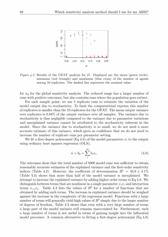
88 Which sensitivity analysis method should I use for my ABM?
Figure 4.5: Results of the OFAT analysis for D. Displayed are the mean (green circle),minimum (red triangle) and maximum (blue cross) of the number of agentsamong 10 replicates. The dashed line represents the nominal value.
for n0 for the global sensitivity analysis. The reduced range has a larger number ofruns with positive outcomes, but also contains runs where the population goes extinct.
For each sample point, we use 5 replicate runs to estimate the variation of themodel output due to stochasticity. To limit the computational expense this numberof replicates is smaller than the 10 replicates for the OFAT. The mean output varianceover replicates is 0.88% of the output variance over all samples. The variance due tostochasticity is thus negligible compared to the variance due to parameter variationsand unexplained variance cannot be attributed to the stochasticity inherent in themodel. Since the variance due to stochasticity is so small, we do not need a moreaccurate estimate of this variance, which gives us confidence that we do not need toincrease the number of replicate runs per parameter setting.
We fit a first-degree polynomial (Eq 4.8) of the model parameters xi to the outputusing ordinary least squares regression (OLS),
n = b0 +
m∑i
bixi. (4.8)
The outcomes show that the total number of 5000 model runs was sufficient to obtainreasonably accurate estimates of the explained variance and the first-order sensitivityindices (Table 4.2). However, the coefficient of determination R2 = 43.9 ± 4.1%(Table 4.3) shows that more than half of the model variance is unexplained. Weattempt to increase the explained variance by adding higher order terms to Eq 4.8. Wedistinguish between terms that are nonlinear in a single parameter xixi and interactionterms x∼ixj . Table 4.3 lists the values of R2 for a number of functions that areobtained by adding such terms. The increase in explained variance should be weighedagainst the increase in the complexity of the regression model. Functions with a largenumber of terms will generally yield high values of R2 simply due to the larger numberof degrees of freedom. Table 4.3 shows that even with a very large number of termsa large part of the model variance still remains unaccounted for. Furthermore, sucha large number of terms is not useful in terms of gaining insight into the influentialmodel processes. A common alternative to fitting a first-degree polynomial (Eq 4.8)
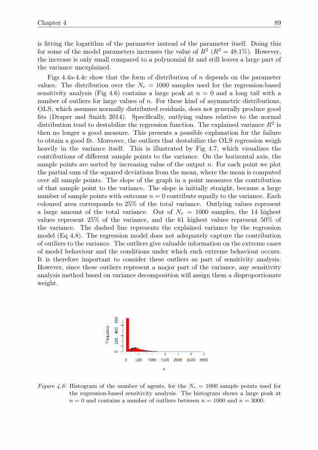
Chapter 4 89
is fitting the logarithm of the parameter instead of the parameter itself. Doing thisfor some of the model parameters increases the value of R2 (R2 = 48.1%). However,the increase is only small compared to a polynomial fit and still leaves a large part ofthe variance unexplained.
Figs 4.4a-4.4c show that the form of distribution of n depends on the parametervalues. The distribution over the Nr = 1000 samples used for the regression-basedsensitivity analysis (Fig 4.6) contains a large peak at n = 0 and a long tail with anumber of outliers for large values of n. For these kind of asymmetric distributions,OLS, which assumes normally distributed residuals, does not generally produce goodfits (Draper and Smith 2014). Specifically, outlying values relative to the normaldistribution tend to destabilize the regression function. The explained variance R2 isthen no longer a good measure. This presents a possible explanation for the failureto obtain a good fit. Moreover, the outliers that destabilize the OLS regression weighheavily in the variance itself. This is illustrated by Fig 4.7, which visualizes thecontributions of different sample points to the variance. On the horizontal axis, thesample points are sorted by increasing value of the output n. For each point we plotthe partial sum of the squared deviations from the mean, where the mean is computedover all sample points. The slope of the graph in a point measures the contributionof that sample point to the variance. The slope is initially straight, because a largenumber of sample points with outcome n = 0 contribute equally to the variance. Eachcoloured area corresponds to 25% of the total variance. Outlying values representa large amount of the total variance. Out of Nr = 1000 samples, the 14 highestvalues represent 25% of the variance, and the 61 highest values represent 50% ofthe variance. The dashed line represents the explained variance by the regressionmodel (Eq 4.8). The regression model does not adequately capture the contributionof outliers to the variance. The outliers give valuable information on the extreme casesof model behaviour and the conditions under which such extreme behaviour occurs.It is therefore important to consider these outliers as part of sensitivity analysis.However, since these outliers represent a major part of the variance, any sensitivityanalysis method based on variance decomposition will assign them a disproportionateweight.
Figure 4.6: Histogram of the number of agents, for the Nr = 1000 sample points used forthe regression-based sensitivity analysis. The histogram shows a large peak atn = 0 and contains a number of outliers between n = 1000 and n = 3000.

90 Which sensitivity analysis method should I use for my ABM?
Table 4.2: First-order indices according to Eq 4.8. The confidence intervals are based on abootstrap sample of size 10,000. Only parameters with at least 1.0% explainedvariance are included. We also report the standardized regression coefficientsβi = bi
σ(n)σ(xi)
. Here the standard deviation σ(n) is computed from the outputsample of the sensitivity analysis and the standard deviation σ(xi) is given bythe input distribution of the parameter xi (see e.g. Cariboni et al. (2007)). Thestandardized regression coefficients measure the strength as well as the directionof the effect of the parameter on the output.
Par. k r Em Rmax Eh c D TotalSr 20.0%
±3.8%
9.1%±3.0%
5.7%±2.6%
4.1%±2.2%
3.3%±1.9%
1.6%±1.4%
1.0%±1.2%
45.5%±4.1%
β 0.43 0.29 -0.24 0.23 -0.18 0.23 0.10 -
Table 4.3: R2 for various polynomial regression models with increasing number of terms. Asignificant increase in the explained variance is obtained by adding terms to theregression model, but this should be weighed against the increased complexityof the regression model. The table shows a large number of terms is needed tosignificantly increase the explained variance.
order ofnonlinearities 1st 2nd 3rd 1st 2nd 1st 2nd 3rdorder ofinteractions - - - 2nd 2nd 3rd 3rd 3rdnumber ofcoefficients 16 31 46 121 136 576 591 606R2 45.5% 49.9% 51.2% 63.7% 67.7% 65.5% 69.0% 70.0%
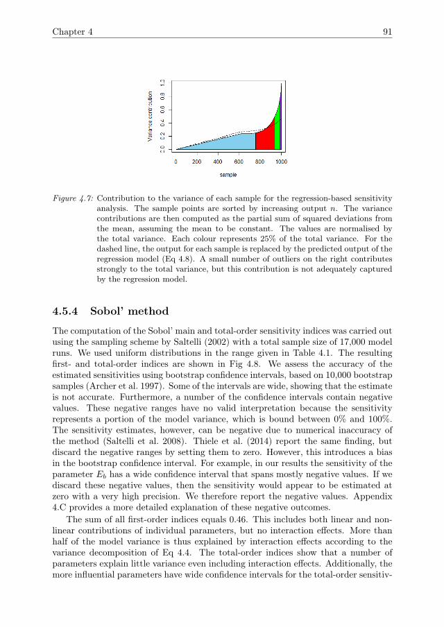
Chapter 4 91
Figure 4.7: Contribution to the variance of each sample for the regression-based sensitivityanalysis. The sample points are sorted by increasing output n. The variancecontributions are then computed as the partial sum of squared deviations fromthe mean, assuming the mean to be constant. The values are normalised bythe total variance. Each colour represents 25% of the total variance. For thedashed line, the output for each sample is replaced by the predicted output of theregression model (Eq 4.8). A small number of outliers on the right contributesstrongly to the total variance, but this contribution is not adequately capturedby the regression model.
4.5.4 Sobol’ method
The computation of the Sobol’ main and total-order sensitivity indices was carried outusing the sampling scheme by Saltelli (2002) with a total sample size of 17,000 modelruns. We used uniform distributions in the range given in Table 4.1. The resultingfirst- and total-order indices are shown in Fig 4.8. We assess the accuracy of theestimated sensitivities using bootstrap confidence intervals, based on 10,000 bootstrapsamples (Archer et al. 1997). Some of the intervals are wide, showing that the estimateis not accurate. Furthermore, a number of the confidence intervals contain negativevalues. These negative ranges have no valid interpretation because the sensitivityrepresents a portion of the model variance, which is bound between 0% and 100%.The sensitivity estimates, however, can be negative due to numerical inaccuracy ofthe method (Saltelli et al. 2008). Thiele et al. (2014) report the same finding, butdiscard the negative ranges by setting them to zero. However, this introduces a biasin the bootstrap confidence interval. For example, in our results the sensitivity of theparameter Eb has a wide confidence interval that spans mostly negative values. If wediscard these negative values, then the sensitivity would appear to be estimated atzero with a very high precision. We therefore report the negative values. Appendix4.C provides a more detailed explanation of these negative outcomes.
The sum of all first-order indices equals 0.46. This includes both linear and non-linear contributions of individual parameters, but no interaction effects. More thanhalf of the model variance is thus explained by interaction effects according to thevariance decomposition of Eq 4.4. The total-order indices show that a number ofparameters explain little variance even including interaction effects. Additionally, themore influential parameters have wide confidence intervals for the total-order sensitiv-
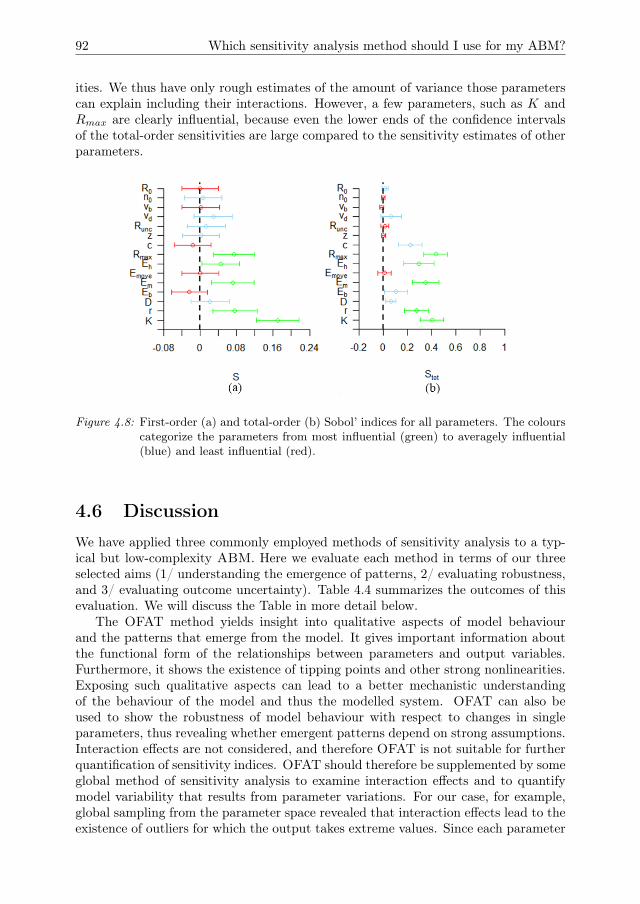
92 Which sensitivity analysis method should I use for my ABM?
ities. We thus have only rough estimates of the amount of variance those parameterscan explain including their interactions. However, a few parameters, such as K andRmax are clearly influential, because even the lower ends of the confidence intervalsof the total-order sensitivities are large compared to the sensitivity estimates of otherparameters.
Figure 4.8: First-order (a) and total-order (b) Sobol’ indices for all parameters. The colourscategorize the parameters from most influential (green) to averagely influential(blue) and least influential (red).
4.6 DiscussionWe have applied three commonly employed methods of sensitivity analysis to a typ-ical but low-complexity ABM. Here we evaluate each method in terms of our threeselected aims (1/ understanding the emergence of patterns, 2/ evaluating robustness,and 3/ evaluating outcome uncertainty). Table 4.4 summarizes the outcomes of thisevaluation. We will discuss the Table in more detail below.
The OFAT method yields insight into qualitative aspects of model behaviourand the patterns that emerge from the model. It gives important information aboutthe functional form of the relationships between parameters and output variables.Furthermore, it shows the existence of tipping points and other strong nonlinearities.Exposing such qualitative aspects can lead to a better mechanistic understandingof the behaviour of the model and thus the modelled system. OFAT can also beused to show the robustness of model behaviour with respect to changes in singleparameters, thus revealing whether emergent patterns depend on strong assumptions.Interaction effects are not considered, and therefore OFAT is not suitable for furtherquantification of sensitivity indices. OFAT should therefore be supplemented by someglobal method of sensitivity analysis to examine interaction effects and to quantifymodel variability that results from parameter variations. For our case, for example,global sampling from the parameter space revealed that interaction effects lead to theexistence of outliers for which the output takes extreme values. Since each parameter
Chapter 4 93
is only varied individually and not in combination with other parameters, OFAT isrelatively cheap in terms of computational costs. At 10 replicates for 11 parametervalues, we need 110 model runs per parameter, or 1650 runs in total. This cost couldstill be lowered by decreasing the number of replicates.
Regression-based sensitivity analysis is a global method based on variance decom-position. A major limitation for application to sensitivity analysis of ABMs is that itdepends on the structure of the model whether a good decomposition can be obtainedby regression. In our case a good fit (with R2 > 0.9) was not obtained even usinga third-order polynomial function because of the existence of outlying values as wellas regions of parameter space where the output goes to zero. This corresponds toprevious reporting difficulties by Burgers et al. (2010) on finding a well-fitted func-tion for an ABM of trading agents. They attributed these difficulties to the inherentcomplexity of the model. We agree with this assessment, where we explicitly add thatin our case the lack of fit is better understood by considering the results we obtainedby first performing the OFAT. The lack of fit resulting from the inherent complexityof ABMs limits the usefulness of regression-based sensitivity analysis for these mod-els, as the systems which they are used to model are complex adaptive systems thatare characterized by the existence of nonlinear interactions and feedbacks, multiplelevels of model behaviour, and emergent properties. These characteristics compli-cate and obscure the relations between the model inputs and outputs and are thusnot straightforwardly captured by a regression function. Even though the regressionfunction does not yield a good fit, however, regression-based sensitivity analysis mightprove useful in selecting influential parameters for further analysis based on the sen-sitivity indices or regression coefficients. The computational costs of regression-basedsensitivity analysis lie somewhere in between OFAT and the Sobol’ method. Forour test-case 1000 parameter settings with 5 replicates each were sufficient to obtainreasonably accurate estimates of the first-order indices.
The Sobol’ method does not use fitted functions, but instead decomposes thevariance based directly on a sample from the parameter space (Saltelli et al. 2008).The method aims to quantify the output variability based on this variance decom-position. Whereas the variance has a clear interpretation for normal distributions,it is not a good measure of variability for distributions that are skewed or containoutliers (Swinscow 1997). This problem is illustrated by Fig 4.7, which shows thatthe output variance of our test case is inflated by a few outlying sample points. Themethod is therefore not suitable for quantifying outcome variability of ABMs withoutput distributions that have outliers, are skewed, or strongly deviate in other waysfrom the normal distribution (Liu et al. 2006). Another drawback of the method isthat the method does not allow for the possibility to distinguish between mechanisticexplanations on why a parameter is influential. For example, in our test case theharvesting cost shows up as an influential parameter (Fig 4.8b), but it is unclearwhether it has some effect on outlying values, or causes collapse of the population,or affects the number of agents for positive population sizes. In contrast, the OFATresults show that it causes population collapse and affects the number of agents forpositive populations, but such specific findings are lost in the Sobol’ method becausesensitivities are aggregated over the full parameter space (Rakovec et al. 2014). Assuch, the method also does not reveal the robustness of model patterns to parameterchanges within this space. Out of the methods we tested, the Sobol’ method has the

94 Which sensitivity analysis method should I use for my ABM?
largest computational costs. With a total of 17.000 model runs, the estimates of thesensitivity indices have wide confidence intervals. For a number of parameters theseintervals included negative values, which have no valid interpretation.
In light of these results we recommend OFAT as the starting point for any sen-sitivity analysis of an ABM, in particular when one wants to gain insight into themechanisms and patterns that ABMs produce, which is a typical goal of many socialsimulation studies. This recommendation seemingly contradicts the one by Saltelliet al. (2008) and Ligmann-Zielinska et al. (2014), who suggest the use of the Sobol’method for model analysis. However, our study suggests that standard methods ofglobal sensitivity analysis do not adequately address the issues that are relevant for theanalysis of ABMs, such as the existence of multiple levels, nonlinear interactions andfeedbacks, and emergent properties, as effectively as OFAT. Obviously any OFATcan be supplemented with a global method to investigate interaction effects, giventhat certain conditions are met, namely that the output distribution is and remainssufficiently similar to a normal distribution, regression fits have a high R2, and con-fidence intervals have positive bounds. Some promising advancements in other fieldsmight prove useful for ABM applications. These include a hybrid local-global sensi-tivity method that examines the distribution of explained variances over portions ofthe parameter space (Rakovec et al. 2014) and alternative sensitivity measures basedon entropy instead of variance (Liu et al. 2006, Auder and Iooss 2008).

Chapter 4 95
Tab
le4.
4:Evaluationof
threediffe
rent
metho
dsof
sensitivityan
alysis
interm
sof
diffe
rent
aims.
Exa
minepa
tterns
OFAT
Show
stheeff
ectof
individu
alpa
rameter
chan
geson
emergent
pat-
terns.
Gives
insigh
tinto
mod
elmecha
nics
byrevealingtipp
ing
points
andotherno
nlinearities.
+
Regression-ba
sed
Con
denses
AB
Mou
tput
into
descriptiverelation
ships,which
yield
insigh
tinto
mod
elbe
haviou
r.How
ever,the
relation
shipsarevalid
only
iftheregression
mod
elfitswelltothe
AB
M.
+/-
Sobo
l’Con
siders
only
theaveraged
effectof
parametersover
thewho
lepa
rameter
space,
andthereforedo
esno
texplorediffe
rent
patterns
withinthis
space.
-
Exa
mine
robu
st-
ness
OFAT
Show
srobu
stness
ofpa
tterns
toindividu
alpa
rameter
chan
ges.
How
ever,interaction
effects
areno
tinclud
ed.
-
Regression-ba
sed
Ifago
odfit
isfoun
d,then
thedescriptiverelation
shipsgive
insigh
tinto
therobu
stness
andcanaccoun
tforinteractioneff
ects.
-
Sobo
l’Doesno
tinvestigatetherobu
stness
ofcertainou
tcom
es,o
nlythe
effects
-
Qua
ntify
outcom
evariab
ility
due
topa
rameters
OFAT
Doesno
texam
inethis
variab
ility,b
ecau
sethis
requ
ires
consider-
ationof
interactioneff
ects.
-
Regression-ba
sed
Ifago
odfit
isfoun
d,then
theou
tput
varian
ceisdecompo
sedinto
term
sattributed
todiffe
rent
(com
bina
tion
sof)pa
rameters.
-
Sobo
l’Decom
posestheou
tput
varian
ceinto
term
sattributed
todiffe
rent
(com
bina
tion
sof)pa
rameters.
+/-
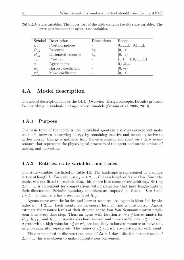
96 Which sensitivity analysis method should I use for my ABM?
Table 4.5: State variables. The upper part of the table contains the site state variables. Thelower part contains the agent state variables.
Symbol Description Dimensions Rangei, j Position indices - 0,1,...,L; 0,1,...,LRi,j Resource kg [0,→〉Rai,j Estimated resource kg [0,→〉xa Position - (0,1,...,L;0,1,...,L)a Agent index - 0,1,2,...wah Harvest coefficient - [0,→〉wam Move coefficient - [0,→〉
4.A Model description
The model description follows the ODD (Overview, Design concepts, Details) protocolfor describing individual- and agent-based models (Grimm et al. 2006, 2010).
4.A.1 Purpose
The basic topic of the model is how individual agents in a spatial environment maketrade-offs between conserving energy by remaining inactive and becoming active togather energy. Energy is gathered from the environment and spent on a daily main-tenance that represents the physiological processes of the agent and on the actions ofmoving and harvesting.
4.A.2 Entities, state variables, and scales
The state variables are listed in Table 4.5. The landscape is represented by a squarelattice of length L. Each site i, j(i, j = 1, 2, ..., L) has a length of ∆x = 1km. Since themodel was not fitted to realistic data, this choice is to some extent arbitrary. Setting∆x = 1, is convenient for computations with parameters that have length-units intheir dimensions. Periodic boundary conditions are imposed, so that i + L = i andj + L = j. Each site has a resource level Ri,j .
Agents move over the lattice and harvest resource. An agent is identified by theindex a = 1, 2, .... Each agents has an energy level Ea and a location xa. Agentsestimate the resource levels at their site and at the four Von Neumann nearest neigh-bour sites every time-step. Thus, an agent with location xa = i, j has estimates forRi,j , Ri±1,j and Ri,j±1. Agents also have harvest and move coefficients, wah and wam.Agents with a high value for wah or wam are less likely to harvest resource or move to aneighbouring site respectively. The values of wah and wam are constant for each agent.
Time is modelled in discrete time steps of ∆t = 1 day. Like the distance scale of∆x = 1, this was chosen to make computations convenient.
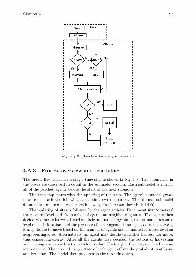
Chapter 4 97
Figure 4.9: Flowchart for a single time-step.
4.A.3 Process overview and scheduling
The model flow chart for a single time-step is shown in Fig 4.9. The submodels inthe boxes are described in detail in the submodel section. Each submodel is run forall of the patches/agents before the start of the next submodel.
The time-step starts with the updating of the sites. The ‘grow’ submodel growsresource on each site following a logistic growth equation. The ‘diffuse’ submodeldiffuses the resource between sites following Fick’s second law (Fick 1855).
The updating of sites is followed by the agent actions. Each agent first ‘observes’the resource level and the number of agents on neighbouring sites. The agents thendecide whether to harvest, based on their internal energy state, the estimated resourcelevel on their location, and the presence of other agents. If an agent does not harvest,it may decide to move based on the number of agents and estimated resource level onneighbouring sites. Alternatively, an agent may decide to neither harvest nor move,thus conserving energy. After all the agents have decided, the actions of harvestingand moving are carried out in random order. Each agent then pays a fixed energymaintenance. The internal energy state of each agent affects the probabilities of dyingand breeding. The model then proceeds to the next time-step.

98 Which sensitivity analysis method should I use for my ABM?
4.A.4 Design conceptsBasic principles
The model considers agents that move and harvest in a spatial environment. Basedon their internal state and the state of the environment agents may decide to moveto a new location, to harvest from the present location, or to wait for a better op-portunity. Harvested resource is converted to internal energy, which is used to paydaily maintenance. The energy for maintenance The acts of moving and harvestingalso cost energy. The decisions to move and harvest are based on both the internalenergy state of the agent and the state of the environment.
Emergence
We consider the total population size ntot and the values of the harvest and movecoefficients wah and wam averaged over the population as emerging variables at themacro-level.
Adaptation
Agents adapt their behaviour to changes in their internal state or in their environment.Agents with low levels of internal energy tend to harvest resource with a higherprobability. Agents also tend to harvest if the resource level on their site is high andthe number of other agents on the site is low.
Agents consider the state of the sites in the Von Neumann neighbourhood in theirdecisions to move to neighbouring sites. Agents are more likely to harvest if theresource level on their current site is high and there are few other agents on this site.Agents are more likely to move to sites with high resource levels and few other agents.
Objectives
The first objective of each agent is to gather sufficient resource to ensure its ownsurvival. The second objective is to accumulate sufficient energy to breed.
Learning
Individual agents do not change their adaptive traits over time. However, the distri-bution of these traits over the population may change due to selection. When agentsbreed, their offspring inherit the parents’ values of wah and wam with some randomvariation. If, for example, agents with a low value wam reproduce more frequentlyoften on average, then low values will become increasingly common over time.
Prediction
Agents tend to move less often to sites that are occupied by one or more other agents,based on the prediction that those other agents may harvest resource from the site.Agents tend to harvest more often at their present location if neighbouring locationsare occupied by other agents that might move to the resource. Agents also tend tomove to sites with high resource levels, predicting that the resource level will remainhigh and can be harvested. If an agent finds the present conditions unsuitable for

Chapter 4 99
harvesting, that agent may decide to wait before taking action, expecting that theconditions will improve in the future.
Sensing
Agents sense their own internal energy. Each time step, agents assess the amount ofresource on their current location and the four sites that compose the Von Neumannneighbourhood. However, agents do not sense the exact amount of resource becausethere is some random error. Agents also sense the presence of any other agents withinthe Von Neumann neighbourhood, without any error.
Interaction
Indirect interactions between agents occur through the competition for resource. Inaddition, agents are less likely to move to or harvest at sites that contain other agents.This is a form of direct interaction. Agents are also more likely to harvest on theirpresent site if neighbours are occupying the neighbouring sites. The basic modelformulation does not include further direct interactions between agents in order forthe model to function as a benchmark.
Stochasticity
The decisions of agents to harvest at the present location or to move to a neighbouringsite are based on smooth probability functions. The functions take as input thenumber of agents and the perceived amount of resource within the Von Neumannneighbourhood. The perceived amount of resource differs from the actual amount byan amount that is drawn from a normal distribution. Birth and death of agents arealso stochastic, but based on the internal energies of agents. If an agents breeds, theoffspring inherit the values of wah and w
am with a small random variation. Furthermore,
the agents’ initial locations, energies and values of wah and wam are also stochastic.
Observation
Three output variables are collected: the total number of agents n and the averagesof wah and wam over all agents. All output variables are recorded at each time-step.
4.A.5 Initialization
All sites are initialized with resource levels equal to R0 times carrying capacity. Theinitial number of agents is specified as a parameter, n0. Each agent is placed on arandom site with an internal energy that is drawn from a uniform distribution between0 and the minimum energy that is needed for procreation. The initial values of wah andwam are drawn from a uniform distribution between 0 and 1. The default parametervalues of the model are listed in Table 4.6.
4.A.6 Input data
The model does not use input data to represent time-varying processes.

100 Which sensitivity analysis method should I use for my ABM?
Table 4.6: List of used symbols in the model description. The upper part contains generalnotation, the middle part model variables and the lower part model parameters
Symbol Description Units/range Defaultvalue
i, j Site indices 1,2,...,L -L Lattice size - 33T Time index day -a Agent index - -∆t Time-step size day 1∆x Site length km 1Ea Initial energy J -N Total number of agents 0,1,2, ... -ni,j Number of agents on site i, j 0,1,2, ... -Rh Harvested resource kg -Ri,j Resource on site i, j kg -Rai,j Observed resource by agent a kg -wah Harvest coefficient - -wam Move coefficient - -xa Location of agent a (0, 1, ...L; 0, 1, ...L) -c Efficiency J kg−1 0.9D Diffusion coefficient km2day−1 0.1Eb Birth energy J 5Eh Harvest cost J 0.1Em Cost of energy maintenance J 0.1Emove Move cost J 0.5K Carrying capacity kg 2n0 Initial number of agents 0,1,2, ... 100r Growth rate s−1 0.1R0 Initial resource 0-1 (proportion of
K)1
Rmax Maximum harvest kg 0.5Runc Uncertainty of resource estimations kg 0.1vb Birth coefficient J−1 10vd Mortality coefficient J−1 10z Variation in offspring traits [0,→〉 0.2
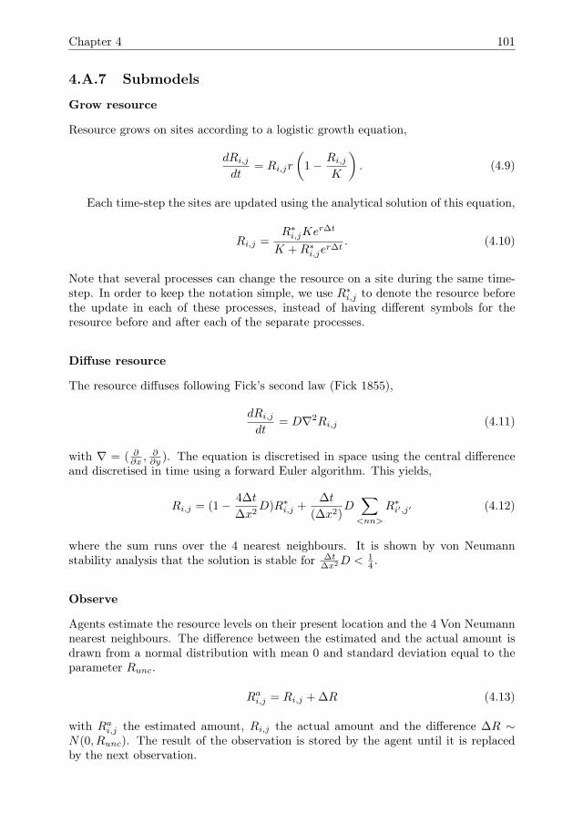
Chapter 4 101
4.A.7 Submodels
Grow resource
Resource grows on sites according to a logistic growth equation,
dRi,jdt
= Ri,jr
(1− Ri,j
K
). (4.9)
Each time-step the sites are updated using the analytical solution of this equation,
Ri,j =R∗i,jKe
r∆t
K +R∗i,jer∆t
. (4.10)
Note that several processes can change the resource on a site during the same time-step. In order to keep the notation simple, we use R∗i,j to denote the resource beforethe update in each of these processes, instead of having different symbols for theresource before and after each of the separate processes.
Diffuse resource
The resource diffuses following Fick’s second law (Fick 1855),
dRi,jdt
= D∇2Ri,j (4.11)
with ∇ = ( ∂∂x ,
∂∂y ). The equation is discretised in space using the central difference
and discretised in time using a forward Euler algorithm. This yields,
Ri,j = (1− 4∆t
∆x2D)R∗i,j +
∆t
(∆x2)D∑<nn>
R∗i′,j′ (4.12)
where the sum runs over the 4 nearest neighbours. It is shown by von Neumannstability analysis that the solution is stable for ∆t
∆x2D < 14 .
Observe
Agents estimate the resource levels on their present location and the 4 Von Neumannnearest neighbours. The difference between the estimated and the actual amount isdrawn from a normal distribution with mean 0 and standard deviation equal to theparameter Runc.
Rai,j = Ri,j + ∆R (4.13)
with Rai,j the estimated amount, Ri,j the actual amount and the difference ∆R ∼N(0, Runc). The result of the observation is stored by the agent until it is replacedby the next observation.

102 Which sensitivity analysis method should I use for my ABM?
Harvest?
The decision of whether to harvest is based on the current internal energy of the agentand the amount of resource that the agent estimates to be present on the site. Thecurrent internal energy is compared with the energy maintenance per time-step,
H(Ea) =Ea
Em− 1. (4.14)
A small value of H indicates that the agent has a low internal energy and needs toharvest soon (i.e. the agent is hungry). If H is negative, then the agent must harvestto survive for another time-step. An agent compares perceived resource on its presentsite to the maximum possible harvest Rmax, which is constant,
G(R∗ai,j , ni,j) = 1−R∗ai,j
ni,jRmax. (4.15)
The resource that the agent expects to harvest is given by the estimated amount ofresource on the patch divided by the total number of agents on the patch. If G isclose to 1, then the expected harvest is small. If G is close to zero, then the agentexpects to harvest close to the maximum possible amount. The final probability toharvest is computed based on the functions H and G,
P aharvest = e−wahHG (4.16)
where wah represents the internal tendency of the individual agent to harvest. Thusan agent is likely to harvest if it is hungry, if it sees a good opportunity for makinga harvest, and if it has a high internal tendency. Since the functions h and g aredimensionless, the state variable wah is also dimensionless. Note that the probabilityof harvesting goes to one if the agent is very hungry, or if the expected harvest isequal to the maximum possible harvest.
Move?
When deciding whether or not to move, an agent predicts how much resource itexpects to obtain at its current site and at the four nearest neighbouring sites. Forits current site i, j the agent expects that the resource will be shared evenly amongthe agents on that site,
Eaexp,i,j =cRi,jni,j
. (4.17)
For a neighbouring site, the agent expects that it will share the resource with theagents already present at the site. The agent also considers that it will first have tospend energy to move to a neighbouring site before harvesting there. Thus, the netexpected energy gain for the neighbouring site is equal to the expected harvest minusthe cost of moving to the site,
Eaexp,k,l =cRk,lnk,l
− Emove. (4.18)
Chapter 4 103
The expected energy gain of the current site is then compared with that of the nearestneighbour with the highest expected gain. Based on this comparison, the probabilityof moving is computed
Pmove = e−wamEi,j/Ek,l . (4.19)
Thus, an agent is likely to move if the expected energy gain is higher on a neigh-bouring site than on the present location. Since both the expected harvests have thedimensions of energy, the variable wam is dimensionless. This variable represents thedifferences between agents in their likeliness to move.
Harvest
The harvest is carried out by updating the amount of resource on the harvested sitei, j and the internal energy level of the harvesting agent. The agent harvests anyresource present on the site up to a maximum of Rmax. The new amount of resourceis thus Ri,j = R∗i,j−Rh, with R∗i,j the amount before harvesting and Rh the harvestedamount,
Rh =
{R∗i,j if R∗i,j < RmaxRmax if R∗i,j > Rmax
(4.20)
. The cost of harvesting Eh is deducted from the internal energy of the agent and theharvested resource is converted with efficiency c and added to the internal energy,
Ea = E∗a + cRh − Eh. (4.21)
Move
The agent moves to the nearest neighbour with the highest value of Rai,j
ni,j. The location
of the agent is updated to the new site.
Maintenance
For each agent, the daily energy cost of maintenance is deducted from the internalenergy,
Ea = E∗a − Em. (4.22)
If the internal energy of the agent is lower than the maintenance costs, it will becomenegative after paying maintenance. Because the ‘pay maintenance’ submodel is im-mediately followed by the ‘die?’ submodel, the agent will then die without taking anyfurther actions.
Die?
Every time-step, agents have a probability of dying or breeding, based on their internalenergy. The probability of dying is
Pdie(Ea) = e−vdE
a
. (4.23)
Thus, the probability of dying goes to one as Ea goes to zero.

104 Which sensitivity analysis method should I use for my ABM?
Die
If an agent dies it is removed from the simulation.
Breed?
If an agent does not die, it has a probability of breeding,
Pbreed(Ea) = 1− e−vb(Ea−Eb) (4.24)
If Ea < Eb then the probability is set to zero. The submodel determines whether theagent will breed based on this probability.
Breed
If an agent breeds, it is replaced by two new agents. The energy of the parent issplit evenly among the two offspring. The values of wah and wam are inherited bythe offspring with some random deviation. The deviation is drawn from a uniformdistribution between −z and z. In some cases, the resulting value of wah and wam canbe negative. It is then set to zero instead.
4.B OFAT resultsThe results of the OFAT analysis are shown in Fig 4.10.
4.C Consequences of the choice of sampling designIn the Sobol’ method, the computation of the sensitivity
Vi = Vxi(Ex∼i
(y|xi)) (4.25)
consists of the evaluation of two integrals over the parameter space. Firstly, we keepthe parameter xi fixed and compute the expectation value over all other parameters,
Ex∼i (y|xi) =
∫f(x1, x2, ..., xk)
k∏j 6=i
pxj (xj)dxj (4.26)
where the function y = f(x1, x2, ..., xk) gives the model output as a function of theparameters and pxj
(xj) is the probability distribution of the parameter xj . Secondly,we compute the variance of Eq 4.26 over all values of
Vxi(Ex∼i
(y|xi)) =
∫ (E2x∼i
(y|xi))pxi
(xi)dxi − E(y)2 (4.27)
where ∼ i indicates ‘not i’. Here we have used the law of total expectation to write∫(Ex∼i
(y|xi)) pxi(xi)dxi = E(y)2. (4.28)
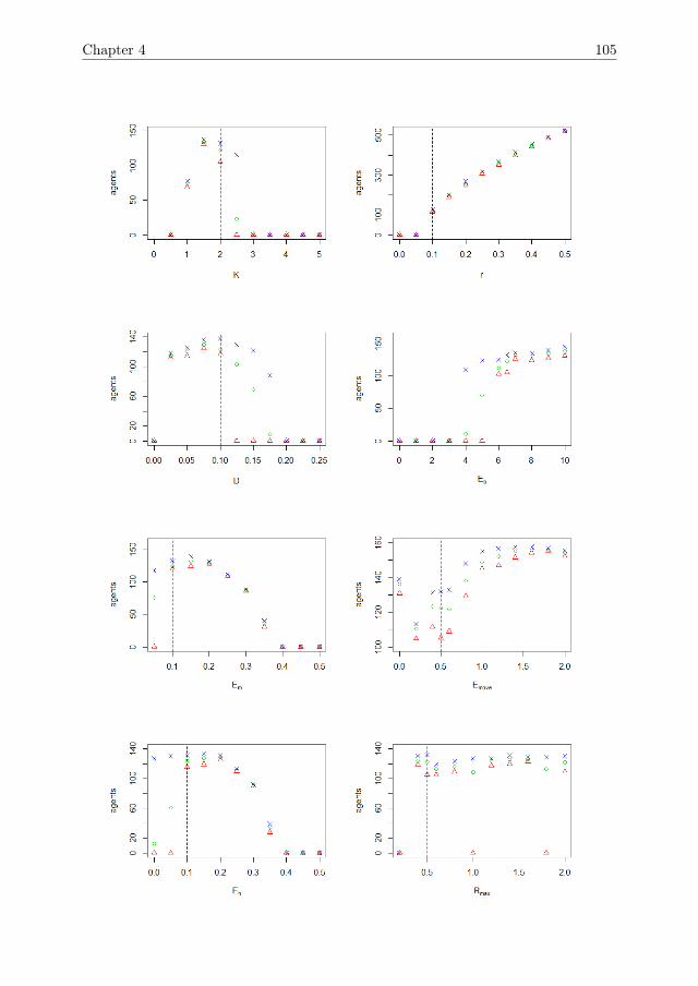
Chapter 4 105
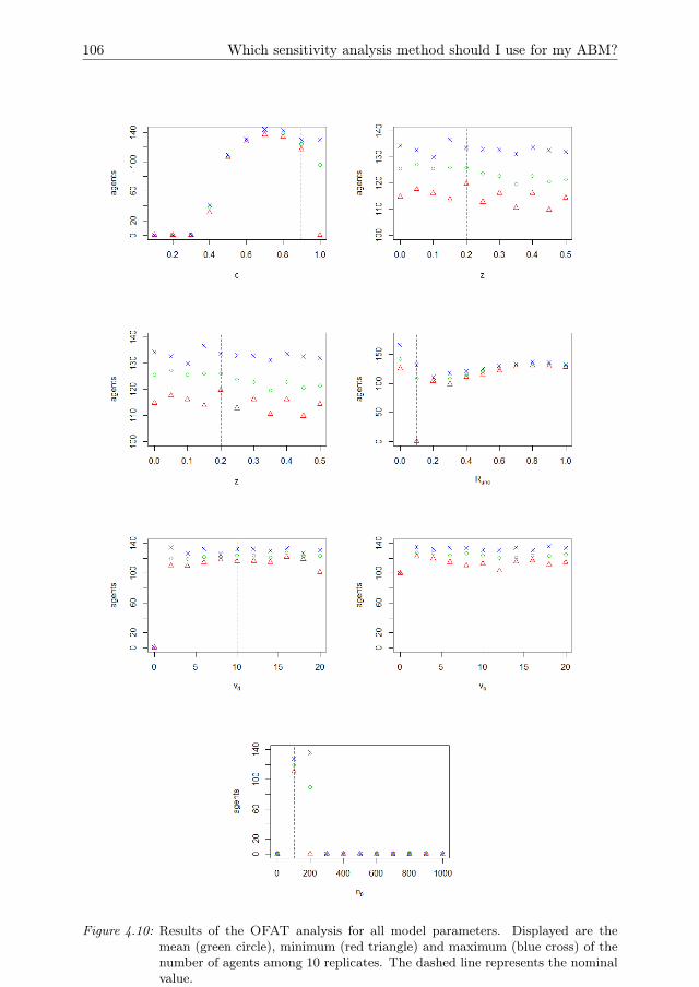
106 Which sensitivity analysis method should I use for my ABM?
Figure 4.10: Results of the OFAT analysis for all model parameters. Displayed are themean (green circle), minimum (red triangle) and maximum (blue cross) of thenumber of agents among 10 replicates. The dashed line represents the nominalvalue.
Chapter 4 107
For ABMs we usually have no analytic expression for f(x1, x2, ..., xk). Instead weobtain the function value for a given set of parameter values by running the ABM.Eq 4.25 therefore cannot be evaluated analytically, but is estimated using samplingmethods. The most straightforward method to compute these integrals uses a full-factorial design (Fig 4.11). Every parameter then takes a number of set values andall the possible combinations of parameter values are sampled. The expectation value(Eq 4.26) is then computed for each value of xi by summing over all values for theother parameters. The variance (Eq 4.27) is computed over the possible values of xi.The required number of models runs is equal to N = nmi , where ni is the numberof values for each parameter and m the number of parameters. This is feasible onlyfor models with a small number of parameters. For the test case discussed in thispaper, we have m = 15. For ni = 5, this would require N ≈ 3.05 ∗ 1010 modelruns, which is outside the range that we can realistically perform. This problem isnot straightforwardly solved by using a Latin Hypercube sample (Fig 4.11), becausewe then have only a single sample point for any value of xi and cannot compute theexpectation value over different values of xi. A number of designs have therefore beensuggested to estimate Eq 4.25 based on fewer model runs (e.g. Cukier et al. (1978),Tarantola et al. (2006), Saltelli (2002)). We use the design by Saltelli (2002). For thisdesign, we rewrite the first term on the right side of Eq 4.27 (see Saltelli (2002) forproof).∫ (
E2x∼i
(y|xi))pxi
(xi)dxi = (4.29)∫f(x1, x2, ..., xk)f(x′1, x
′2, ..., x
′i−1, xi, x
′i+1, ...x
′k)
k∏j=1
pxj (xj)
k∏j 6=i
pxj (x′j)dx′j (4.30)
Observe that all xj have an alternative value x′j except the one for which we computethe sensitivity (indicated by xi). The integral computes the expectation value off(x1, x2, ..., xk)f(x′1, x
′2, ..., x
′i−1, xi, x
′i+1.., x
′k) and is evaluated using a single Monte
Carlo sample. We randomly draw a number of sample points from the parameterdistributions (Fig 4.11) and run the model for each point to obtain a number ofmodel outcomes
yj = f(xj1, xj2, ..., x
jk), y′j = f(x′j1 , x
′j2 , ..., x
′ji−1, x
ji , x′ji+1, ...x
′jk ) for j = 1, 2, ..., Ns
(4.31)
with Ns the chosen sample size. The integral is then estimated by averaging the prod-uct yjy′j over all sample points. Eq 4.30 implies that the partial variance of Eq 4.25 isequal to the covariance between f(x1, x2, ..., xk) and f(x′1, x
′2, ..., x
′i−1, xi, xi+ 1′.., x′k),
where the primed parameter values are sampled independently from the values with-out a prime. However, the estimates for the covariance can yield negative valuesbecause of this independent sampling. In contrast, the partial variance can never benegative because it consists of squared deviations. Thus, the appearance of negativevalues for the estimates of the sensitivity indices results from the inaccuracy of thecovariance estimate. This inaccuracy is often substantial, as we illustrate below fora simple example. This may be because the integral of Eq 4.30 is computed overa parameter space of dimension 2k − 1. The introduction of the primed parameter
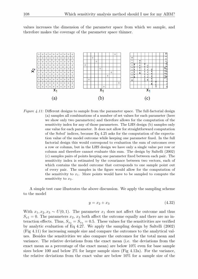
108 Which sensitivity analysis method should I use for my ABM?
values increases the dimension of the parameter space from which we sample, andtherefore makes the coverage of the parameter space thinner.
Figure 4.11: Different designs to sample from the parameter space. The full-factorial design(a) samples all combinations of a number of set values for each parameter (herewe show only two parameters) and therefore allows for the computation of thesensitivity index for any of those parameters. The LHS design (b) samples onlyone value for each parameter. It does not allow for straightforward computationof the Sobol’ indices, because Eq 4.25 asks for the computation of the expecta-tion value of the model outcome while keeping one parameter fixed. In the fullfactorial design this would correspond to evaluation the sum of outcomes overa row or column, but in the LHS design we have only a single value per row orcolumn and therefore cannot evaluate this sum. The design by Saltelli (2002)(c) samples pairs of points keeping one parameter fixed between each pair. Thesensitivity index is estimated by the covariance between two vectors, each ofwhich contains the model outcome that corresponds to one sample point outof every pair. The samples in the figure would allow for the computation ofthe sensitivity to x1. More points would have to be sampled to compute thesensitivity to x2.
A simple test case illustrates the above discussion. We apply the sampling schemeto the model
y = x2 + x3 (4.32)
With x1, x2, x3 ∼ U(0, 1). The parameter x1 does not affect the outcome and thusSx1 = 0. The parameters x2, x3 both affect the outcome equally and there are no in-teraction effects. Thus, Sx2 = Sx3 = 0.5. These values for the sensitivities are verifiedby analytic evaluation of Eq 4.27. We apply the sampling design by Saltelli (2002)(Fig 4.11) for increasing sample size and compare the outcomes to the analytical val-ues. Besides the sensitivities we also compare the outcomes for the total mean andvariance. The relative deviations from the exact mean (i.e. the deviations from theexact mean as a percentage of the exact mean) are below 10% even for base samplesizes below 100 and below 2% for larger sample sizes (Fig 4.12a). For the variance,the relative deviations from the exact value are below 10% for a sample size of the

Chapter 4 109
order and are within a few percent for larger sample sizes (Fig 4.12b). The sensitivityestimates, however, are less accurate (Fig 4.12c). We encounter deviations from theexact values between 10-20% even for base sample sizes close to 5000. We cannotplot the relative deviation for Sx1
because the analytic value is zero. The absoluteestimates for the sensitivity reveal that the distribution is centred around the truevalue zero; The number of negative outcomes is approximately equal to the numberof positive outcomes.
The example model of Eq 4.32 shows that even for a very simple test model, alarge sample size is needed to accurately estimate sensitivities following the designby Saltelli (Saltelli 2002). This matches the finding that the sensitivity estimates forour ABM have wide confidence intervals (Fig 4.7). Furthermore, negative sensitivityestimates are not unlikely, especially for parameters that have little effect on the modeloutcomes. These negative estimates indicate the inaccuracy of the sampling designfor estimating the sensitivities. We therefore suggest to report negative sensitivityestimates explicitly. For example, some of the sensitivity indices that we report inFig 4.7 for our ABM test case have confidence intervals that are largely negative.Discarding these negative ranges by setting them to zero might give the reader anunrealistic confidence in the accuracy of the estimates.
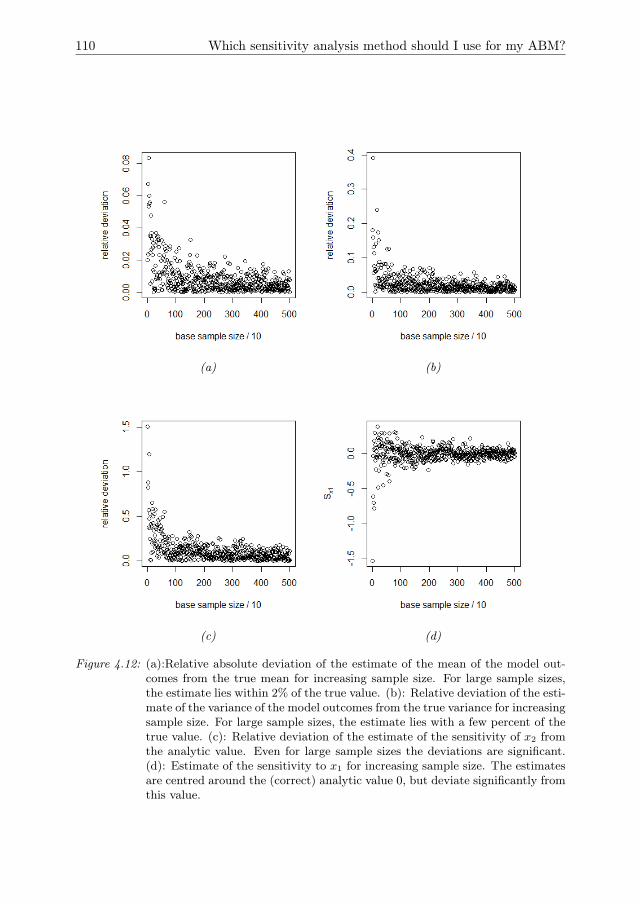
110 Which sensitivity analysis method should I use for my ABM?
(a) (b)
(c) (d)
Figure 4.12: (a):Relative absolute deviation of the estimate of the mean of the model out-comes from the true mean for increasing sample size. For large sample sizes,the estimate lies within 2% of the true value. (b): Relative deviation of the esti-mate of the variance of the model outcomes from the true variance for increasingsample size. For large sample sizes, the estimate lies with a few percent of thetrue value. (c): Relative deviation of the estimate of the sensitivity of x2 fromthe analytic value. Even for large sample sizes the deviations are significant.(d): Estimate of the sensitivity to x1 for increasing sample size. The estimatesare centred around the (correct) analytic value 0, but deviate significantly fromthis value.

Chapter 5
Resilience through adaptation
G.A. ten Broeke, G.A.K. van Voorn, A. Ligtenberg, J. Molenaar.PlosOne, 12(2):e0171833.
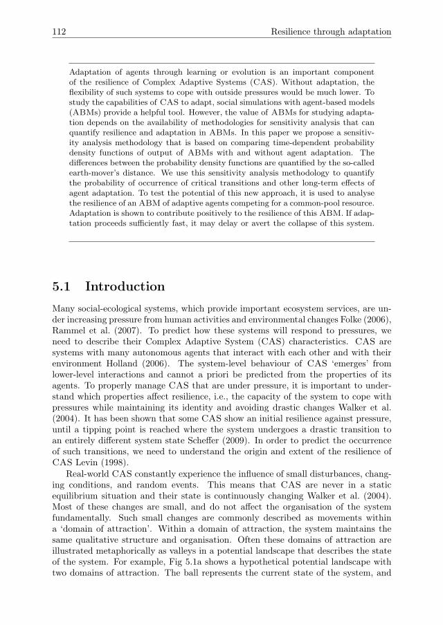
112 Resilience through adaptation
Adaptation of agents through learning or evolution is an important componentof the resilience of Complex Adaptive Systems (CAS). Without adaptation, theflexibility of such systems to cope with outside pressures would be much lower. Tostudy the capabilities of CAS to adapt, social simulations with agent-based models(ABMs) provide a helpful tool. However, the value of ABMs for studying adapta-tion depends on the availability of methodologies for sensitivity analysis that canquantify resilience and adaptation in ABMs. In this paper we propose a sensitiv-ity analysis methodology that is based on comparing time-dependent probabilitydensity functions of output of ABMs with and without agent adaptation. Thedifferences between the probability density functions are quantified by the so-calledearth-mover’s distance. We use this sensitivity analysis methodology to quantifythe probability of occurrence of critical transitions and other long-term effects ofagent adaptation. To test the potential of this new approach, it is used to analysethe resilience of an ABM of adaptive agents competing for a common-pool resource.Adaptation is shown to contribute positively to the resilience of this ABM. If adap-tation proceeds sufficiently fast, it may delay or avert the collapse of this system.
5.1 Introduction
Many social-ecological systems, which provide important ecosystem services, are un-der increasing pressure from human activities and environmental changes Folke (2006),Rammel et al. (2007). To predict how these systems will respond to pressures, weneed to describe their Complex Adaptive System (CAS) characteristics. CAS aresystems with many autonomous agents that interact with each other and with theirenvironment Holland (2006). The system-level behaviour of CAS ‘emerges’ fromlower-level interactions and cannot a priori be predicted from the properties of itsagents. To properly manage CAS that are under pressure, it is important to under-stand which properties affect resilience, i.e., the capacity of the system to cope withpressures while maintaining its identity and avoiding drastic changes Walker et al.(2004). It has been shown that some CAS show an initial resilience against pressure,until a tipping point is reached where the system undergoes a drastic transition toan entirely different system state Scheffer (2009). In order to predict the occurrenceof such transitions, we need to understand the origin and extent of the resilience ofCAS Levin (1998).
Real-world CAS constantly experience the influence of small disturbances, chang-ing conditions, and random events. This means that CAS are never in a staticequilibrium situation and their state is continuously changing Walker et al. (2004).Most of these changes are small, and do not affect the organisation of the systemfundamentally. Such small changes are commonly described as movements withina ‘domain of attraction’. Within a domain of attraction, the system maintains thesame qualitative structure and organisation. Often these domains of attraction areillustrated metaphorically as valleys in a potential landscape that describes the stateof the system. For example, Fig 5.1a shows a hypothetical potential landscape withtwo domains of attraction. The ball represents the current state of the system, and
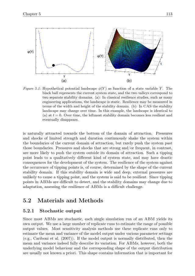
Chapter 5 113
Figure 5.1: Hypothetical potential landscape φ(Y ) as function of a state variable Y . Theblack ball represents the current system state, and the two valleys correspond totwo separate stability domains. (a): In classical resilience studies, such as manyengineering applications, the landscape is static. Resilience may be measured interms of the width and height of the stability domain. (b): In CAS the stabilitylandscape may change over time. In this example, the landscape is identical to(a) at t = 0. Over time, the leftmost stability domain becomes less resilient andeventually disappears.
is naturally attracted towards the bottom of the domain of attraction. Pressuresand shocks of limited strength and duration continuously shake the system withinthe boundaries of the current domain of attraction, but rarely push the system pastthose boundaries. Pressures and shocks that are strong and/or frequent, in contrast,are more likely to push the system outside its domain of attraction. Such a tippingpoint leads to a qualitatively different kind of system state, and may have drasticconsequences for the development of the system. The resilience of the system againstthe occurrence of tipping points is, of course, determined by the shape of the currentstability domain. If this stability domain is wide and deep, external pressures areunlikely to cause a tipping point, and the system is said to be resilient. Since tippingpoints in ABMs are difficult to detect, and the stability domains may change due toadaptation, assessing the resilience of ABMs is a difficult challenge.
5.2 Materials and Methods
5.2.1 Stochastic output
Since most ABMs are stochastic, each single simulation run of an ABM yields itsown output. We use a large number of replicate runs to estimate the range of possibleoutput values. Most sensitivity analysis methods use these replicate runs only toestimate the mean and variance of the model output under various parameter settings(e.g., Cariboni et al. (2007)). If the model output is normally distributed, then themean and variance indeed fully describe its variation. For ABMs, however, both theunderlying model behaviour and the corresponding shape of the output distributionare usually not known a priori. This shape contains information that is important for
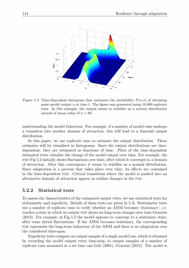
114 Resilience through adaptation
Figure 5.2: Time-dependent histogram that estimates the probability P (n, t) of obtainingsome model output n at time t. The figure was generated using 10.000 replicateruns. In this example, the output seems to stabilise as a normal distributionaround of mean value of n = 90.
understanding the model behaviour. For example, if a number of model runs undergoa transition into another domain of attraction, this will lead to a bimodal outputdistribution.
In this paper, we use replicate runs to estimate the output distribution. Theseestimates will be visualised as histograms. Since the output distributions are time-dependent, they are estimated as functions of time. Plots of the time-dependentestimated pdfs visualise the change of the model output over time. For example, thepdf Fig 5.2 initially shows fluctuations over time, after which it converges to a domainof attraction. After this convergence it seems to stabilise as a normal distribution.Since adaptation is a process that takes place over time, its effects are containedin the time-dependent pdf. Critical transitions where the model is pushed into analternative domain of attraction appear as sudden changes in the pdf.
5.2.2 Statistical tests
To assess the characteristics of the estimated output pdfs, we use statistical tests forstationarity and ergodicity. Details of these tests are given in 5.A. Stationarity testsuse a number of replicate runs to verify whether an ABM becomes ‘stationary’, i.e.reaches a state in which its output pdf shows no long-term changes over time Grazzini(2012). For example, in Fig 5.2 the model appears to converge to a stationary state,after some initial fluctuations. If the ABM becomes stationary, the correspondingpdf represents the long-term behaviour of the ABM and there is no adaptation overthe considered time-span.
Ergodicity tests compare an output sample of a single model run, which is obtainedby recording the model output every time-step, to output samples of a number ofreplicate runs measured at a set time van Lith (2001), Grazzini (2012). The model is

Chapter 5 115
Table 5.1: Description of used symbols.
Symbol Description UnitsD Diffusion coefficient km2day−1
de Earth mover’s distance -dJ Jensen-Shannon distance between histograms -du Euclidian distance between histograms -d(j, k) Distance between bins of histograms (5.B) -Eh Energy cost for an agent to harvest JEm Energy cost for an agent to move Jg(j, k) Flow between bins of histograms (5.B) -Ht Vector used in runs test (5.A) -j, k, l Indices for output values -N Number (observations, model runs,... ) #n Number of agents #Pa(n, t) Normalised histogram of ABM with adaptation -Pb(n, t) Normalised histogram of ABM without adaptation -Qi(t) Adaptation measure for parameter i at time t -Q′i(t) Rate of adaptation over time t−1
T Length of time-series -t Time index dayV Variance -W Statistic used in trend test (5.A) -wharvest Agent’s harvest parameter -wmove Agent’s move parameter -Y Model output variable -z Inheritance parameter -λ Extinction parameter day−1
µ Mean -ρ Increase in pressure -φ Potential J
116 Resilience through adaptation
considered to be ergodic if the null-hypothesis that the output samples are identical isnot rejected. In other words, the stochastic variation between replicates is then equalto the stochastic variation over time of a single model run. A difference betweenthe output samples indicates that the model output contains variation over timethat cannot be attributed to stochasticity, and may indicate that adaptation hastaken place over the considered time-scale. Since only a single model run is used toestimate the time-averaged pdf, ergodicity is a highly attractive property if we wantto explore the model behaviour on very long time-scales. In the following, we willrefer to histograms that are obtained by recording a single model run over successivetimes-steps as time-averaged histograms. We refer to histograms that are recordedover replicate runs as function of time as time-dependent histograms.
Sensitivity measuresIn order to assess how adaptation influences the model output, we need to measurethe sensitivity of the output pdf to the presence of adaptation. We measure thissensitivity by comparing the estimated time-dependent pdfs of the output of modelversions with adaptation Pa(n, t) and without adaptation Pb(n, t). Here n denotes thenumber of agents, which is used throughout this paper as the central model output.To quantify the comparison we use the earth-mover’s distance de Rubner et al. (1998).
For an intuitive interpretation of the earth mover’s distance, consider two pdfsPa(n, t) and Pb(n, t) as amounts of mass that are spread over a distance specifiedby the model output n. The earth-mover’s distance de(Pa(n, t), Pb(n, t)) is then thework required to transform Pa(n, t) into Pb(n, t). Several properties follow from thisinterpretation. Firstly, for all Pa(n, t) and Pb(n, t), de(Pa, Pb) ≥ 0, and de(Pa, Pb) = 0implies that Pa = Pb. Any positive value of de(Pa, Pb) thus indicates a differencebetween the pdfs. Small values indicate that the pdfs are quite similar, and largevalues indicate strong differences between the pdfs. We denote by
Q(t) = de(Pa(n, t), Pb(n, t)) (5.1)
the effects of adaptation at time t. Note that all the used symbols are described inTable 5.1. Q(t) measures the effect of a parameter change, namely the enabling ordisabling of adaptation. Other sensitivity measures based on a comparison betweenoutput pdfs have been previously suggested (e.g. Liu et al. (2006), Auder and Iooss(2008), Borgonovo (2007)). All of these measures are based on the (lack of) overlapbetween those pdfs. For our purposes, these measures are not suitable, becausewe want to measure the effects of adaptation even when there is little or no overlapbetween the pdfs. The earth-mover’s distance allows us to do this, because an increasein the distance between pdfs will result in an increase of the earth-mover’s distance,even when the pdfs do not overlap.
In addition to the effects of adaptation at a specific time, we are also interestedin the rate of adaptation. We calculate the rate of change of Q(t) by computing thedifference between time-steps,
Q′(t) = de(Pa(t), Pb(t))− de(Pa(t−∆t), Pb(t−∆t)), (5.2)
Chapter 5 117
with ∆t small compared to the time-scale of the process. This measure for the rateof adaptation helps to identify periods in time where adaptation proceeds relativelyfast, or where there is little adaptation. For example, adaptation may be influentialon short simulation times, but have little effect on longer simulation times, or theother way around.
5.2.3 Computation of the earth mover’s distanceComputing the earth-mover’s distance between a pair of distributions amounts tofinding the minimal ’work’ needed to change one distribution into the other. We writeg(j, k) for the matrix element that contains the flow between output values j and k,d(j, k) for the distance between the output values, and we consider g(j, k)d(j, k) as thework required to transport g(j, k) from j to k. There are many possible choices for thematrix g to transform one distribution into the other. To compute the earth-mover’sdistance, we minimise g(j, k)d(j, k) over these possible choices Ling and Okada (2007),
de = min
∑(j,k)
g(j, k)d(j, k)
(5.3)
with the constraints
∑k
g(j, k) = Pa(j) ∀j (5.4)∑j
g(j, k) = Pb(k) ∀k (5.5)
g(j, k) ≥ 0 ∀j, k (5.6)
with d(j, k) the distance between j and k, and the indices j and k running overtheir domains. Eq 5.4 and Eq 5.5 ensure that the flow is such that the distributionPa(j) is transformed into Pb(k). Eq 5.6 ensures that mass is moved from Pa(j) toPb(k), and not the other way around. Eq 5.3 ensures that the flow is chosen such tominimise the required ’work’ g(j, k)d(j, k). For two pdfs of a single output variable,this minimisation is accomplished by going through all consecutive pairs of outputvalues, and keeping track of the amount of mass that needs to be transported. 5.Ccontains a sample pseudo-code for this computation. For the computation of defor continuous, or multi-dimensional distributions, we refer to Venkatasubramanian(2013). Packages to compute de are available for various statistical software andprogramming languages.
5.2.4 Method to measure adaptationIn Fig 5.3 we present the scheme of our method to measure adaptation of ABMs.The first step is to prepare an ABM with adaptation, and a version of the sameABM in which this adaptation is disabled. Agent adaptation in our test-case consistsof the selection of agent characteristics for replication or modification Levin (1998).Disabling this selection ensures that there is no adaptation and that the distribution of
118 Resilience through adaptation
agent properties does not change over time. In the ABM with adaptation, the agentproperties may change over time, for example through natural selection, or throughindividual agents learning from past experience or imitation of other agents Holland(2006), Macal (2016). To measure the effects of such adaptations, we compare theoutput of the ABM with adaptation to that of the ABM without adaptation. Therest of the method is composed of steps for analysing the model output and comparingthe estimated output pdfs using Eq 5.1 and Eq 5.2.
Based on a large number of replicate runs, we generate histograms of the outputto estimate the time-dependent output pdfs of the ABM without adaptation Pb andof the adaptive ABM Pa. To measure adaptation, we need to examine how the pdfschange with time. Thus, for each ABM we estimate the pdf at multiple points intime. Based on these data, we use stationarity tests to verify whether the ABMs reachan equilibrium, or continue to change over the considered time-scale. Furthermore,for each ABM we also perform a single model run with a very long simulation time totest the ergodicity. If the stationarity test reveals that the ABM reaches a stationarystate, then the time after which this state is reached is used as a starting point forthe ergodicity test, but the ergodicity test explores longer simulation times than thestationarity test. If the model is ergodic, then we may conclude that no adaptationtakes place.
Once the pdfs of the ABMs with adaptation and without adaptation have beenanalysed, we proceed by comparing them to quantify the effects of adaptation. Thedifference between the pdfs is quantified using Q (Eq 5.1). In addition to measuringthe effects of adaptation over a specified time-span, we also measure the rate ofadaptation using Q′ (Eq 5.2). This rate of adaptation is especially relevant in thecontext of resilience. For the resilience of the system to be influenced by adaptation,the rate of adaptation must be sufficiently fast to respond to pressures. For example,if a pressure to the system increases very fast, then adaptation must also be able tooccur fast in order to affect the consequences of the pressure.
5.2.5 Model description
We consider a previously published test-case, in which adaptation emerges througha process of natural selection. An overview of all model parameters and their de-fault values is given in 5.D. For a full model description we refer to Ten Broeke,Van Voorn and Ligtenberg (2016). Here we focus mainly on the mechanism for adap-tation. Fig 5.4 presents a flow chart of the model. The test-case is a resource-agentsystem, in which the agents compete for a renewable common-pool resource in a spa-tial environment. The spatial environment is composed of a grid of square sites, onwhich resource grows and diffuses, and on which agents live (Fig 5.5). Every time-step, each agent estimates the amounts of resource and observes the number of agentson its present location and the four neighbouring sites. Based on this information,it decides whether to harvest on its present site, to move to a neighbouring site, orto stay inactive. These decisions are stochastic, but the probabilities are influencedby the agent’s own (decreasing) internal energy state (‘hunger’) as well as the stateof the local surroundings, including the presence of resources (‘food availability’) andother agents (‘crowding’). Harvesting or moving costs energy, in addition to theenergy consumed by basic maintenance every time-step. There are thus trade-offs be-
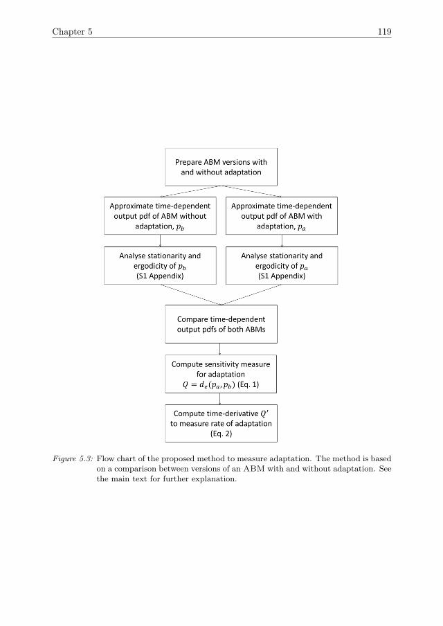
Chapter 5 119
Figure 5.3: Flow chart of the proposed method to measure adaptation. The method is basedon a comparison between versions of an ABM with and without adaptation. Seethe main text for further explanation.
120 Resilience through adaptation
tween harvesting, moving, and remaining inactive, which form the basis of the agent’sdecision-making process. At the end of each time-step, all agents have a probabilityof dying and of reproducing, based on their internal energy state. Low values for theinternal energy increase the probability of dying, whereas high values increase theprobability of reproducing.
Each agent has two agent parameters that affect its decisions to harvest or move:wharvest and wmove. Besides these parameters, the probabilities of harvesting ormoving also depend on the weighted average of a few factors, including the agent’sinternal energy, the resource on its site and the resource on its neighbouring sites.This average, multiplied by wharvest or wmove, is input to a function that determinesthe probability. If wharvest = 0 the agent will choose to harvest with probability1. Similarly, if wmove = 0 the agent will choose to move with probability 1. Largerparameter values decrease the probabilities. For the initial agent population, thevalues of these parameters are drawn from a uniform probability distribution. Thevalues remain constant over the lifetime of an agent. Upon reproduction, an agentpasses on its values of wharvest and wmove to its offspring, with a small randomdeviation. The distribution of the parameter values across the population may thuschange over time through a process of natural selection. Since the probability ofreproducing is higher for agents with a high internal energy, agents that are successfulat gathering energy are also more likely to reproduce and pass on their characteristics.Agents that are not successful at gathering energy, in contrast, are more likely to diewithout reproducing. Parameter values that increase an agent’s success at gatheringenergy are thus passed on more frequently, whereas parameter values that decreaseits success tend to disappear from the population. Over time, the distribution acrossthe population of the parameters values will thus move towards values that increasesuccess at gathering energy. This change in the distribution represents the process ofthe population adapting to its environment.
To obtain a non-adaptive version of the ABM, we disable the inheritance of agentcharacteristics. In the non-adaptive version, when a new agent is added to the sys-tem, its values of wharvest and wmove are chosen according to the same probabilitydistribution that is used for the initial agent population. Thus, in this version thereare no long-term changes in the distribution of wharvest and wmove across the agentpopulation.
5.3 Results
Non-adaptive ABM
In the following sections, we will consider the agent population size n as the centralmodel output. Following the scheme in Fig 5.3, we estimate the output histogram ofthe ABM without adaptation in the default parameter setting. Detailed results of thestatistical tests are given in 5.C. Model runs in the default parameter setting showthat the output initially oscillates, but stabilises around t = 1000. Between t = 1000and t = 2000, the mean of the output across replicates is nearly constant on average,with short-term fluctuations. Due to these fluctuations, stationarity tests show thatthe output is not stationary. To test whether there are any long-term trends, weaverage the output over short time-windows and test whether the series of window
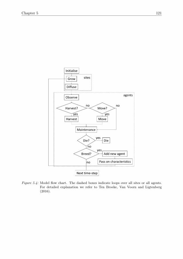
Chapter 5 121
Figure 5.4: Model flow chart. The dashed boxes indicate loops over all sites or all agents.For detailed explanation we refer to Ten Broeke, Van Voorn and Ligtenberg(2016).
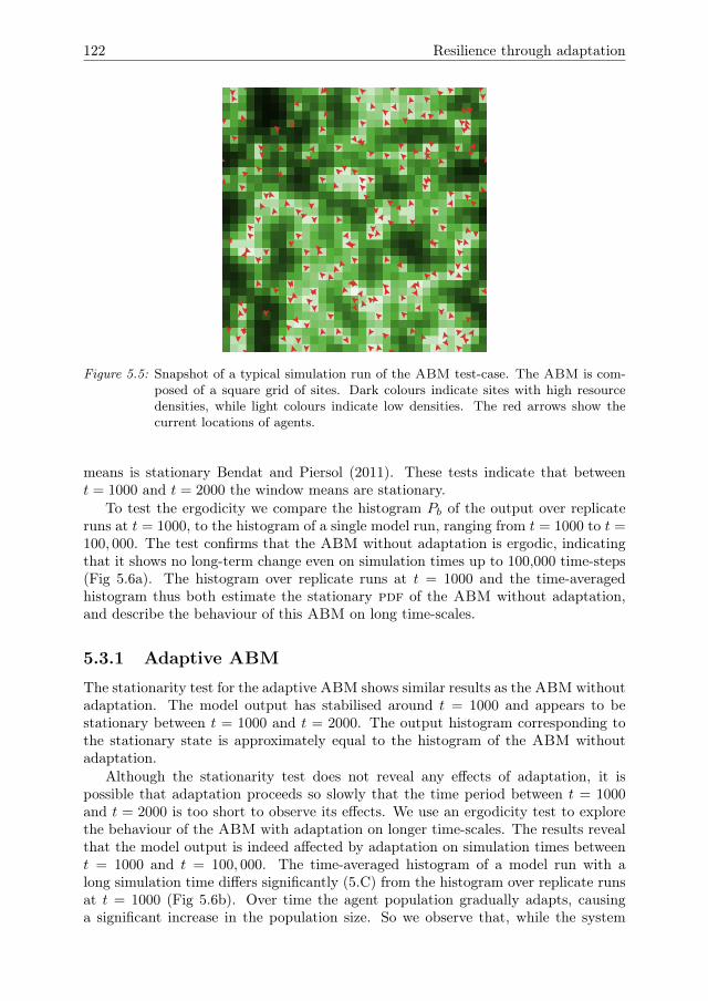
122 Resilience through adaptation
Figure 5.5: Snapshot of a typical simulation run of the ABM test-case. The ABM is com-posed of a square grid of sites. Dark colours indicate sites with high resourcedensities, while light colours indicate low densities. The red arrows show thecurrent locations of agents.
means is stationary Bendat and Piersol (2011). These tests indicate that betweent = 1000 and t = 2000 the window means are stationary.
To test the ergodicity we compare the histogram Pb of the output over replicateruns at t = 1000, to the histogram of a single model run, ranging from t = 1000 to t =100, 000. The test confirms that the ABM without adaptation is ergodic, indicatingthat it shows no long-term change even on simulation times up to 100,000 time-steps(Fig 5.6a). The histogram over replicate runs at t = 1000 and the time-averagedhistogram thus both estimate the stationary pdf of the ABM without adaptation,and describe the behaviour of this ABM on long time-scales.
5.3.1 Adaptive ABM
The stationarity test for the adaptive ABM shows similar results as the ABM withoutadaptation. The model output has stabilised around t = 1000 and appears to bestationary between t = 1000 and t = 2000. The output histogram corresponding tothe stationary state is approximately equal to the histogram of the ABM withoutadaptation.
Although the stationarity test does not reveal any effects of adaptation, it ispossible that adaptation proceeds so slowly that the time period between t = 1000and t = 2000 is too short to observe its effects. We use an ergodicity test to explorethe behaviour of the ABM with adaptation on longer time-scales. The results revealthat the model output is indeed affected by adaptation on simulation times betweent = 1000 and t = 100, 000. The time-averaged histogram of a model run with along simulation time differs significantly (5.C) from the histogram over replicate runsat t = 1000 (Fig 5.6b). Over time the agent population gradually adapts, causinga significant increase in the population size. So we observe that, while the system
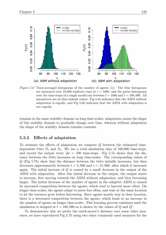
Chapter 5 123
Figure 5.6: Time-averaged histograms of the number of agents (n). The blue histogramsare measured over 10,000 replicate runs at t = 1000, and the green histogramsover the time-steps of a single model run between t = 1000 and t = 100, 000. Allparameters are at their default values. Fig 5.6a indicates that the ABM withoutadaptation is ergodic, and Fig 5.6b indicates that the ABM with adaptation isnot ergodic.
remains in the same stability domain on long time-scales, adaptation causes the shapeof this stability domain to gradually change over time, whereas without adaptationthe shape of the stability domain remains constant.
5.3.2 Effects of adaptation
To estimate the effects of adaptation we compute Q between the estimated time-dependent pdfs Pa and Pb. We use a total simulation time of 100,000 time-steps,and record the output every ∆t = 100 time-steps. Fig 5.7a shows that the dis-tance between the pdfs increases on long time-scales. The corresponding values ofQ (Fig 5.7b) show that the distance between the pdfs initially increases, but thendecreases approximately between t = 5, 000 and t = 15, 000, after which it increasesagain. The initial increase of Q is caused by a small decrease in the output of theABM with adaptation. After this initial decrease in the output, the output startsto increase, first moving towards the ABM without adaptation, and then becominglarger. The initial decrease of the number of agents in the adaptive ABM is causedby increased competition between the agents, which tend to harvest more often. Onlonger time-scales, the agents adapt to move less often, and wait at the same locationto let the resource grow before harvesting. Since agents mostly stay in their location,there is a decreased competition between the agents, which leads to an increase inthe number of agents on longer time-scales. This learning process continues until thesimulation is stopped at t = 100, 000 as is shown by the values of Q and Q′.
To demonstrate why we prefer the earth-mover’s distance over some other mea-sures, we have reproduced Fig 5.7b using two other commonly used measures for the
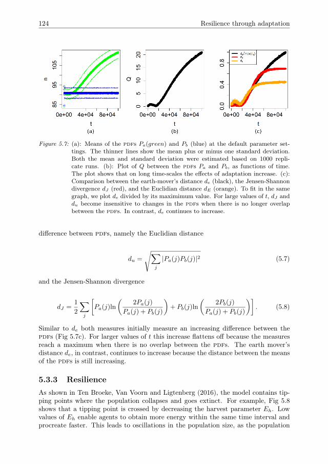
124 Resilience through adaptation
Figure 5.7: (a): Means of the pdfs Pa(green) and Pb (blue) at the default parameter set-tings. The thinner lines show the mean plus or minus one standard deviation.Both the mean and standard deviation were estimated based on 1000 repli-cate runs. (b): Plot of Q between the pdfs Pa and Pb, as functions of time.The plot shows that on long time-scales the effects of adaptation increase. (c):Comparison between the earth-mover’s distance de (black), the Jensen-Shannondivergence dJ (red), and the Euclidian distance dE (orange). To fit in the samegraph, we plot de divided by its maximimum value. For large values of t, dJ anddu become insensitive to changes in the pdfs when there is no longer overlapbetween the pdfs. In contrast, de continues to increase.
difference between pdfs, namely the Euclidian distance
du =
√∑j
|Pa(j)Pb(j)|2 (5.7)
and the Jensen-Shannon divergence
dJ =1
2
∑j
[Pa(j)ln
(2Pa(j)
Pa(j) + Pb(j)
)+ Pb(j)ln
(2Pb(j)
Pa(j) + Pb(j)
)]. (5.8)
Similar to de both measures initially measure an increasing difference between thepdfs (Fig 5.7c). For larger values of t this increase flattens off because the measuresreach a maximum when there is no overlap between the pdfs. The earth mover’sdistance de, in contrast, continues to increase because the distance between the meansof the pdfs is still increasing.
5.3.3 ResilienceAs shown in Ten Broeke, Van Voorn and Ligtenberg (2016), the model contains tip-ping points where the population collapses and goes extinct. For example, Fig 5.8shows that a tipping point is crossed by decreasing the harvest parameter Eh. Lowvalues of Eh enable agents to obtain more energy within the same time interval andprocreate faster. This leads to oscillations in the population size, as the population
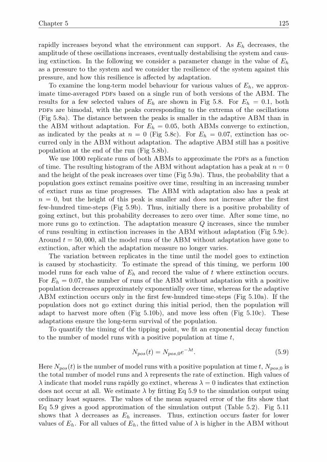
Chapter 5 125
rapidly increases beyond what the environment can support. As Eh decreases, theamplitude of these oscillations increases, eventually destabilising the system and caus-ing extinction. In the following we consider a parameter change in the value of Ehas a pressure to the system and we consider the resilience of the system against thispressure, and how this resilience is affected by adaptation.
To examine the long-term model behaviour for various values of Eh, we approx-imate time-averaged pdfs based on a single run of both versions of the ABM. Theresults for a few selected values of Eh are shown in Fig 5.8. For Eh = 0.1, bothpdfs are bimodal, with the peaks corresponding to the extrema of the oscillations(Fig 5.8a). The distance between the peaks is smaller in the adaptive ABM than inthe ABM without adaptation. For Eh = 0.05, both ABMs converge to extinction,as indicated by the peaks at n = 0 (Fig 5.8c). For Eh = 0.07, extinction has oc-curred only in the ABM without adaptation. The adaptive ABM still has a positivepopulation at the end of the run (Fig 5.8b).
We use 1000 replicate runs of both ABMs to approximate the pdfs as a functionof time. The resulting histogram of the ABM without adaptation has a peak at n = 0and the height of the peak increases over time (Fig 5.9a). Thus, the probability that apopulation goes extinct remains positive over time, resulting in an increasing numberof extinct runs as time progresses. The ABM with adaptation also has a peak atn = 0, but the height of this peak is smaller and does not increase after the firstfew-hundred time-steps (Fig 5.9b). Thus, initially there is a positive probability ofgoing extinct, but this probability decreases to zero over time. After some time, nomore runs go to extinction. The adaptation measure Q increases, since the numberof runs resulting in extinction increases in the ABM without adaptation (Fig 5.9c).Around t = 50, 000, all the model runs of the ABM without adaptation have gone toextinction, after which the adaptation measure no longer varies.
The variation between replicates in the time until the model goes to extinctionis caused by stochasticity. To estimate the spread of this timing, we perform 100model runs for each value of Eh and record the value of t where extinction occurs.For Eh = 0.07, the number of runs of the ABM without adaptation with a positivepopulation decreases approximately exponentially over time, whereas for the adaptiveABM extinction occurs only in the first few-hundred time-steps (Fig 5.10a). If thepopulation does not go extinct during this initial period, then the population willadapt to harvest more often (Fig 5.10b), and move less often (Fig 5.10c). Theseadaptations ensure the long-term survival of the population.
To quantify the timing of the tipping point, we fit an exponential decay functionto the number of model runs with a positive population at time t,
Npos(t) = Npos,0e−λt. (5.9)
HereNpos(t) is the number of model runs with a positive population at time t, Npos,0 isthe total number of model runs and λ represents the rate of extinction. High values ofλ indicate that model runs rapidly go extinct, whereas λ = 0 indicates that extinctiondoes not occur at all. We estimate λ by fitting Eq 5.9 to the simulation output usingordinary least squares. The values of the mean squared error of the fits show thatEq 5.9 gives a good approximation of the simulation output (Table 5.2). Fig 5.11shows that λ decreases as Eh increases. Thus, extinction occurs faster for lowervalues of Eh. For all values of Eh, the fitted value of λ is higher in the ABM without
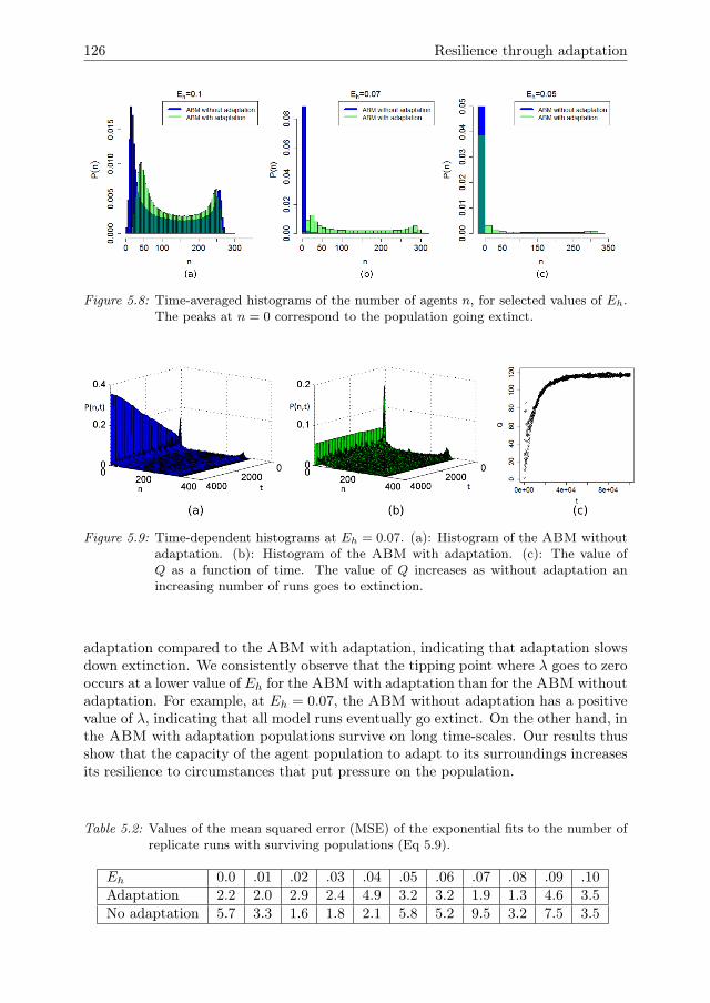
126 Resilience through adaptation
Figure 5.8: Time-averaged histograms of the number of agents n, for selected values of Eh.The peaks at n = 0 correspond to the population going extinct.
Figure 5.9: Time-dependent histograms at Eh = 0.07. (a): Histogram of the ABM withoutadaptation. (b): Histogram of the ABM with adaptation. (c): The value ofQ as a function of time. The value of Q increases as without adaptation anincreasing number of runs goes to extinction.
adaptation compared to the ABM with adaptation, indicating that adaptation slowsdown extinction. We consistently observe that the tipping point where λ goes to zerooccurs at a lower value of Eh for the ABM with adaptation than for the ABM withoutadaptation. For example, at Eh = 0.07, the ABM without adaptation has a positivevalue of λ, indicating that all model runs eventually go extinct. On the other hand, inthe ABM with adaptation populations survive on long time-scales. Our results thusshow that the capacity of the agent population to adapt to its surroundings increasesits resilience to circumstances that put pressure on the population.
Table 5.2: Values of the mean squared error (MSE) of the exponential fits to the number ofreplicate runs with surviving populations (Eq 5.9).
Eh 0.0 .01 .02 .03 .04 .05 .06 .07 .08 .09 .10Adaptation 2.2 2.0 2.9 2.4 4.9 3.2 3.2 1.9 1.3 4.6 3.5No adaptation 5.7 3.3 1.6 1.8 2.1 5.8 5.2 9.5 3.2 7.5 3.5
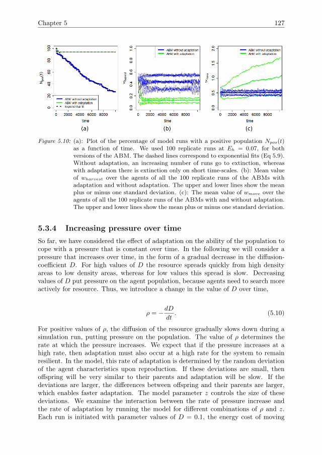
Chapter 5 127
Figure 5.10: (a): Plot of the percentage of model runs with a positive population Npos(t)as a function of time. We used 100 replicate runs at Eh = 0.07, for bothversions of the ABM. The dashed lines correspond to exponential fits (Eq 5.9).Without adaptation, an increasing number of runs go to extinction, whereaswith adaptation there is extinction only on short time-scales. (b): Mean valueof wharvest over the agents of all the 100 replicate runs of the ABMs withadaptation and without adaptation. The upper and lower lines show the meanplus or minus one standard deviation. (c): The mean value of wmove over theagents of all the 100 replicate runs of the ABMs with and without adaptation.The upper and lower lines show the mean plus or minus one standard deviation.
5.3.4 Increasing pressure over timeSo far, we have considered the effect of adaptation on the ability of the population tocope with a pressure that is constant over time. In the following we will consider apressure that increases over time, in the form of a gradual decrease in the diffusion-coefficient D. For high values of D the resource spreads quickly from high densityareas to low density areas, whereas for low values this spread is slow. Decreasingvalues of D put pressure on the agent population, because agents need to search moreactively for resource. Thus, we introduce a change in the value of D over time,
ρ = −dDdt. (5.10)
For positive values of ρ, the diffusion of the resource gradually slows down during asimulation run, putting pressure on the population. The value of ρ determines therate at which the pressure increases. We expect that if the pressure increases at ahigh rate, then adaptation must also occur at a high rate for the system to remainresilient. In the model, this rate of adaptation is determined by the random deviationof the agent characteristics upon reproduction. If these deviations are small, thenoffspring will be very similar to their parents and adaptation will be slow. If thedeviations are larger, the differences between offspring and their parents are larger,which enables faster adaptation. The model parameter z controls the size of thesedeviations. We examine the interaction between the rate of pressure increase andthe rate of adaptation by running the model for different combinations of ρ and z.Each run is initiated with parameter values of D = 0.1, the energy cost of moving
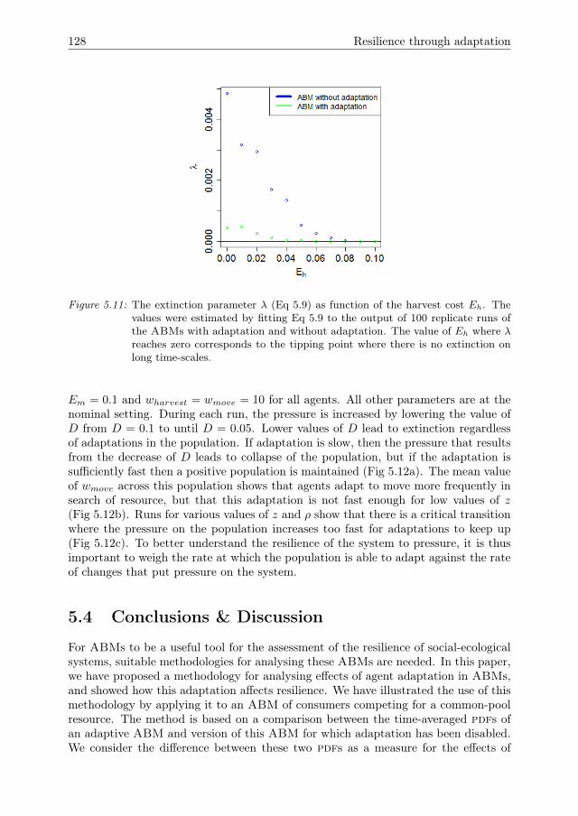
128 Resilience through adaptation
Figure 5.11: The extinction parameter λ (Eq 5.9) as function of the harvest cost Eh. Thevalues were estimated by fitting Eq 5.9 to the output of 100 replicate runs ofthe ABMs with adaptation and without adaptation. The value of Eh where λreaches zero corresponds to the tipping point where there is no extinction onlong time-scales.
Em = 0.1 and wharvest = wmove = 10 for all agents. All other parameters are at thenominal setting. During each run, the pressure is increased by lowering the value ofD from D = 0.1 to until D = 0.05. Lower values of D lead to extinction regardlessof adaptations in the population. If adaptation is slow, then the pressure that resultsfrom the decrease of D leads to collapse of the population, but if the adaptation issufficiently fast then a positive population is maintained (Fig 5.12a). The mean valueof wmove across this population shows that agents adapt to move more frequently insearch of resource, but that this adaptation is not fast enough for low values of z(Fig 5.12b). Runs for various values of z and ρ show that there is a critical transitionwhere the pressure on the population increases too fast for adaptations to keep up(Fig 5.12c). To better understand the resilience of the system to pressure, it is thusimportant to weigh the rate at which the population is able to adapt against the rateof changes that put pressure on the system.
5.4 Conclusions & Discussion
For ABMs to be a useful tool for the assessment of the resilience of social-ecologicalsystems, suitable methodologies for analysing these ABMs are needed. In this paper,we have proposed a methodology for analysing effects of agent adaptation in ABMs,and showed how this adaptation affects resilience. We have illustrated the use of thismethodology by applying it to an ABM of consumers competing for a common-poolresource. The method is based on a comparison between the time-averaged pdfs ofan adaptive ABM and version of this ABM for which adaptation has been disabled.We consider the difference between these two pdfs as a measure for the effects of
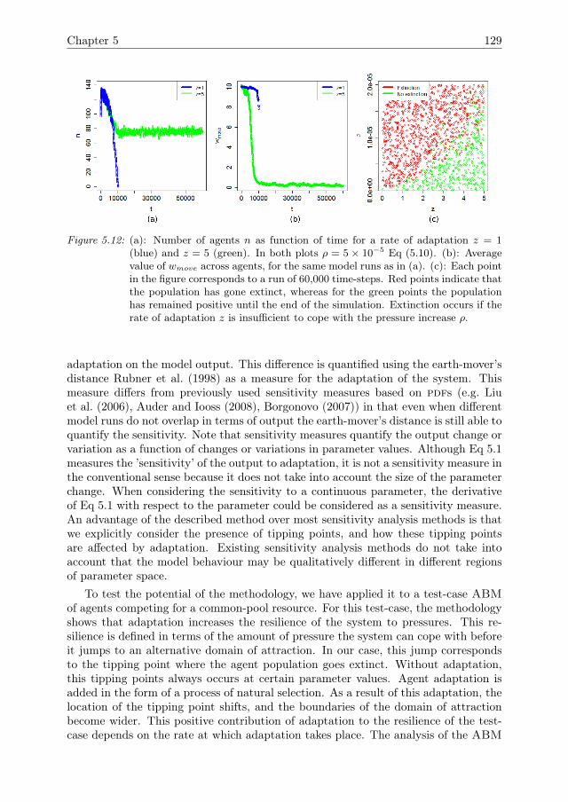
Chapter 5 129
Figure 5.12: (a): Number of agents n as function of time for a rate of adaptation z = 1(blue) and z = 5 (green). In both plots ρ = 5 × 10⁻⁵ Eq (5.10). (b): Averagevalue of wmove across agents, for the same model runs as in (a). (c): Each pointin the figure corresponds to a run of 60,000 time-steps. Red points indicate thatthe population has gone extinct, whereas for the green points the populationhas remained positive until the end of the simulation. Extinction occurs if therate of adaptation z is insufficient to cope with the pressure increase ρ.
adaptation on the model output. This difference is quantified using the earth-mover’sdistance Rubner et al. (1998) as a measure for the adaptation of the system. Thismeasure differs from previously used sensitivity measures based on pdfs (e.g. Liuet al. (2006), Auder and Iooss (2008), Borgonovo (2007)) in that even when differentmodel runs do not overlap in terms of output the earth-mover’s distance is still able toquantify the sensitivity. Note that sensitivity measures quantify the output change orvariation as a function of changes or variations in parameter values. Although Eq 5.1measures the ’sensitivity’ of the output to adaptation, it is not a sensitivity measure inthe conventional sense because it does not take into account the size of the parameterchange. When considering the sensitivity to a continuous parameter, the derivativeof Eq 5.1 with respect to the parameter could be considered as a sensitivity measure.An advantage of the described method over most sensitivity analysis methods is thatwe explicitly consider the presence of tipping points, and how these tipping pointsare affected by adaptation. Existing sensitivity analysis methods do not take intoaccount that the model behaviour may be qualitatively different in different regionsof parameter space.
To test the potential of the methodology, we have applied it to a test-case ABMof agents competing for a common-pool resource. For this test-case, the methodologyshows that adaptation increases the resilience of the system to pressures. This re-silience is defined in terms of the amount of pressure the system can cope with beforeit jumps to an alternative domain of attraction. In our case, this jump correspondsto the tipping point where the agent population goes extinct. Without adaptation,this tipping points always occurs at certain parameter values. Agent adaptation isadded in the form of a process of natural selection. As a result of this adaptation, thelocation of the tipping point shifts, and the boundaries of the domain of attractionbecome wider. This positive contribution of adaptation to the resilience of the test-case depends on the rate at which adaptation takes place. The analysis of the ABM
130 Resilience through adaptation
shows that for a system to be resilient, the rate of adaptation needs to be sufficientlyfast to cope with increasing pressures or changing conditions.
Other authors have discussed ABMs similar to our test-case Burtsev and Turchin(2006), Aubert-Kato et al. (2015), Colon et al. (2015) In Burtsev and Turchin (2006),Aubert-Kato et al. (2015) the focus is mostly on the evolution of behavioural strategiesfor the agents, which are characterised by a neural net. Both studies find that variousstrategies evolve, ranging from greedy to cooperative. In our ABM the range ofpossible strategies is smaller, because the ABM contains only two agents parametersthat are affected by natural selection. For any given parameter setting the modelseems to converge to a dominant strategy, but it depends on the parameter settingwhat this strategy is. For some settings it corresponds to ’greedy’ agents that harvestas often as possible, whereas for other settings it corresponds to agents that harvestless frequently in order to let the resource grow. A possible extension to our modelwould be to include more agent parameters, possibly involving direct interactionsbetween agents such as in Burtsev and Turchin (2006). For the present study, ourmain aim is to examine how agent behaviour affects the resilience of the system as awhole. In Colon et al. (2015) the resilience of different stability domains of an ABMis considered, but here the agent behaviour is completely pre-defined, and the systemdoes not contain adaptation.
In this paper we have considered only adaptation through a process of naturalselection. Adaptation through natural selection typically takes place on long time-scales relative to other types of adaptation. Furthermore, adaptation through naturalselection is reactive in the sense that it that responds to changes in the environment,but cannot respond to changes that agents might foresee in the future. In many CAS,individual agents have the ability to learn from past experiences and to adjust theirbehaviour according to expected future developments. These types of adaptation canbe expected to operate on much shorter time-scales than natural selection Gell-Mann(1994). Future work will include investigating types of adaptation that operate onfaster time-scales, or in which agents adapt proactively based on foreseen changes.Such fast adaptations might lead to an increase in the resilience of the system asagents are able to quickly adapt to situations and respond to pressures. Alternatively,however, they might also destabilise the system, for example when agents mispredicttrends or overspecialise Nelson (2011)).
In this paper, we have analysed the effects of adaptation in a simulated CAS. Theanalysis is based on a comparison between a non-adaptive and an adaptive ABM. Inorder to apply this methodology to a real-life CAS, one thus needs to develop modelversions with and without adaptation. To this end, one needs to assess whetherthe system is adaptive, and what system components and interactions are relevantto understanding this adaptation. Qualitative tools for this kind of assessment areavailable (e.g. Alliance (2010)). The methodology in this paper complements suchresilience assessments by quantifying the resilience of the system using ABMs.
Our results imply that for studies that aim to assess or to enhance the resilience ofsocial-ecological systems, it is relevant to consider the ability of the system to adapt.When combined with suitable methodologies for sensitivity analysis, ABMs can bea helpful tool to test hypotheses on which factors may contribute to the resilience ofsocial-ecological systems (e.g., Heckbert et al. (2014), Janssen and Carpenter (1999),Schlüter and Pahl-Wostl (2007), Schouten et al. (2013)).
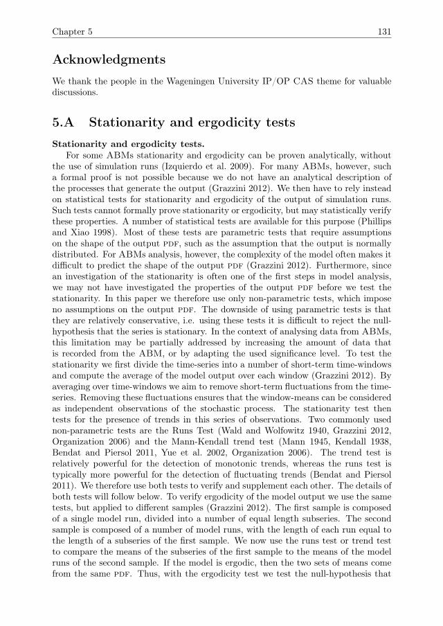
Chapter 5 131
Acknowledgments
We thank the people in the Wageningen University IP/OP CAS theme for valuablediscussions.
5.A Stationarity and ergodicity tests
Stationarity and ergodicity tests.For some ABMs stationarity and ergodicity can be proven analytically, without
the use of simulation runs (Izquierdo et al. 2009). For many ABMs, however, sucha formal proof is not possible because we do not have an analytical description ofthe processes that generate the output (Grazzini 2012). We then have to rely insteadon statistical tests for stationarity and ergodicity of the output of simulation runs.Such tests cannot formally prove stationarity or ergodicity, but may statistically verifythese properties. A number of statistical tests are available for this purpose (Phillipsand Xiao 1998). Most of these tests are parametric tests that require assumptionson the shape of the output pdf, such as the assumption that the output is normallydistributed. For ABMs analysis, however, the complexity of the model often makes itdifficult to predict the shape of the output pdf (Grazzini 2012). Furthermore, sincean investigation of the stationarity is often one of the first steps in model analysis,we may not have investigated the properties of the output pdf before we test thestationarity. In this paper we therefore use only non-parametric tests, which imposeno assumptions on the output pdf. The downside of using parametric tests is thatthey are relatively conservative, i.e. using these tests it is difficult to reject the null-hypothesis that the series is stationary. In the context of analysing data from ABMs,this limitation may be partially addressed by increasing the amount of data thatis recorded from the ABM, or by adapting the used significance level. To test thestationarity we first divide the time-series into a number of short-term time-windowsand compute the average of the model output over each window (Grazzini 2012). Byaveraging over time-windows we aim to remove short-term fluctuations from the time-series. Removing these fluctuations ensures that the window-means can be consideredas independent observations of the stochastic process. The stationarity test thentests for the presence of trends in this series of observations. Two commonly usednon-parametric tests are the Runs Test (Wald and Wolfowitz 1940, Grazzini 2012,Organization 2006) and the Mann-Kendall trend test (Mann 1945, Kendall 1938,Bendat and Piersol 2011, Yue et al. 2002, Organization 2006). The trend test isrelatively powerful for the detection of monotonic trends, whereas the runs test istypically more powerful for the detection of fluctuating trends (Bendat and Piersol2011). We therefore use both tests to verify and supplement each other. The details ofboth tests will follow below. To verify ergodicity of the model output we use the sametests, but applied to different samples (Grazzini 2012). The first sample is composedof a single model run, divided into a number of equal length subseries. The secondsample is composed of a number of model runs, with the length of each run equal tothe length of a subseries of the first sample. We now use the runs test or trend testto compare the means of the subseries of the first sample to the means of the modelruns of the second sample. If the model is ergodic, then the two sets of means comefrom the same pdf. Thus, with the ergodicity test we test the null-hypothesis that
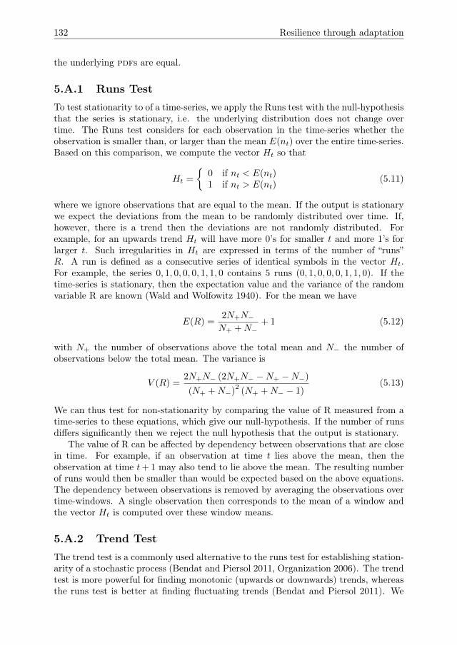
132 Resilience through adaptation
the underlying pdfs are equal.
5.A.1 Runs Test
To test stationarity to of a time-series, we apply the Runs test with the null-hypothesisthat the series is stationary, i.e. the underlying distribution does not change overtime. The Runs test considers for each observation in the time-series whether theobservation is smaller than, or larger than the mean E(nt) over the entire time-series.Based on this comparison, we compute the vector Ht so that
Ht =
{0 if nt < E(nt)1 if nt > E(nt)
(5.11)
where we ignore observations that are equal to the mean. If the output is stationarywe expect the deviations from the mean to be randomly distributed over time. If,however, there is a trend then the deviations are not randomly distributed. Forexample, for an upwards trend Ht will have more 0’s for smaller t and more 1’s forlarger t. Such irregularities in Ht are expressed in terms of the number of “runs”R. A run is defined as a consecutive series of identical symbols in the vector Ht.For example, the series 0, 1, 0, 0, 0, 1, 1, 0 contains 5 runs (0, 1, 0, 0, 0, 1, 1, 0). If thetime-series is stationary, then the expectation value and the variance of the randomvariable R are known (Wald and Wolfowitz 1940). For the mean we have
E(R) =2N+N−N+ +N−
+ 1 (5.12)
with N+ the number of observations above the total mean and N− the number ofobservations below the total mean. The variance is
V (R) =2N+N− (2N+N− −N+ −N−)
(N+ +N−)2
(N+ +N− − 1)(5.13)
We can thus test for non-stationarity by comparing the value of R measured from atime-series to these equations, which give our null-hypothesis. If the number of runsdiffers significantly then we reject the null hypothesis that the output is stationary.
The value of R can be affected by dependency between observations that are closein time. For example, if an observation at time t lies above the mean, then theobservation at time t+ 1 may also tend to lie above the mean. The resulting numberof runs would then be smaller than would be expected based on the above equations.The dependency between observations is removed by averaging the observations overtime-windows. A single observation then corresponds to the mean of a window andthe vector Ht is computed over these window means.
5.A.2 Trend Test
The trend test is a commonly used alternative to the runs test for establishing station-arity of a stochastic process (Bendat and Piersol 2011, Organization 2006). The trendtest is more powerful for finding monotonic (upwards or downwards) trends, whereasthe runs test is better at finding fluctuating trends (Bendat and Piersol 2011). We

Chapter 5 133
will thus use both tests to verify and complement each other. As in the runs test, thenull-hypothesis is that the underlying distribution of a time-series is stationary. Thetrend test is based on the value of,
W =
Nm−1∑t=1
Nm∑t′=t+1
sgn(nt − n′t) (5.14)
where T is the number of observations and
sgn(n) =
−1 if n < 00 if n = 01 if n > 0
(5.15)
For a sufficiently long time-series, W is normally distributed with mean and variance,
E(W ) = 0 (5.16)
V (W ) =1
18Nm(Nm − 1)(2Nm + 5)−
∑g
g(g − 1)(2g + 5) (5.17)
Here the summation∑g runs over all groups of observations that have tied output
values n and g is the number of measurements in each of these groups. These equationsfor the mean and variance describe the null-hypothesis that the actual values of Ware tested against. Similar to the runs Test, the trend is affected when there is adependency between observations that are close in time. We may divide the seriesinto time windows and treat the window averages as individual observations to removesuch dependencies.
5.B Computation of the earth mover’s distance.
Computing the earth-mover’s distance between a pair of distributions amounts tofinding the minimal ’work’ needed to change on distribution into the other. In thispaper, we will deal with pairs of one-dimensional discrete output distributions, Pa(n)and Pb(n), where we have dropped the time-dependency for convenience. The earth-mover’s distance is then written as (Ling and Okada 2007),
de = min
∑(j,k)
g(j, k)d(j, k)
(5.18)
with the constraints, ∑k
g(j, k) = Pa(j)∀j (5.19)∑j
g(j, k) = Pb(k)∀k (5.20)
g(j, k) ≥ 0∀j, k (5.21)
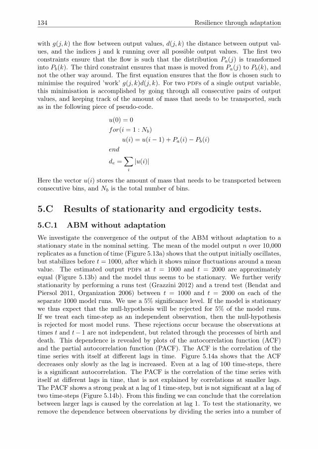
134 Resilience through adaptation
with g(j, k) the flow between output values, d(j, k) the distance between output val-ues, and the indices j and k running over all possible output values. The first twoconstraints ensure that the flow is such that the distribution Pa(j) is transformedinto Pb(k). The third constraint ensures that mass is moved from Pa(j) to Pb(k), andnot the other way around. The first equation ensures that the flow is chosen such tominimise the required ’work’ g(j, k)d(j, k). For two pdfs of a single output variable,this minimisation is accomplished by going through all consecutive pairs of outputvalues, and keeping track of the amount of mass that needs to be transported, suchas in the following piece of pseudo-code.
u(0) = 0
for(i = 1 : Nb)
u(i) = u(i− 1) + Pa(i)− Pb(i)end
de =∑i
|u(i)|
Here the vector u(i) stores the amount of mass that needs to be transported betweenconsecutive bins, and Nb is the total number of bins.
5.C Results of stationarity and ergodicity tests.
5.C.1 ABM without adaptationWe investigate the convergence of the output of the ABM without adaptation to astationary state in the nominal setting. The mean of the model output n over 10,000replicates as a function of time (Figure 5.13a) shows that the output initially oscillates,but stabilizes before t = 1000, after which it shows minor fluctuations around a meanvalue. The estimated output pdfs at t = 1000 and t = 2000 are approximatelyequal (Figure 5.13b) and the model thus seems to be stationary. We further verifystationarity by performing a runs test (Grazzini 2012) and a trend test (Bendat andPiersol 2011, Organization 2006) between t = 1000 and t = 2000 on each of theseparate 1000 model runs. We use a 5% significance level. If the model is stationarywe thus expect that the null-hypothesis will be rejected for 5% of the model runs.If we treat each time-step as an independent observation, then the null-hypothesisis rejected for most model runs. These rejections occur because the observations attimes t and t− 1 are not independent, but related through the processes of birth anddeath. This dependence is revealed by plots of the autocorrelation function (ACF)and the partial autocorrelation function (PACF). The ACF is the correlation of thetime series with itself at different lags in time. Figure 5.14a shows that the ACFdecreases only slowly as the lag is increased. Even at a lag of 100 time-steps, thereis a significant autocorrelation. The PACF is the correlation of the time series withitself at different lags in time, that is not explained by correlations at smaller lags.The PACF shows a strong peak at a lag of 1 time-step, but is not significant at a lag oftwo time-steps (Figure 5.14b). From this finding we can conclude that the correlationbetween larger lags is caused by the correlation at lag 1. To test the stationarity, weremove the dependence between observations by dividing the series into a number of
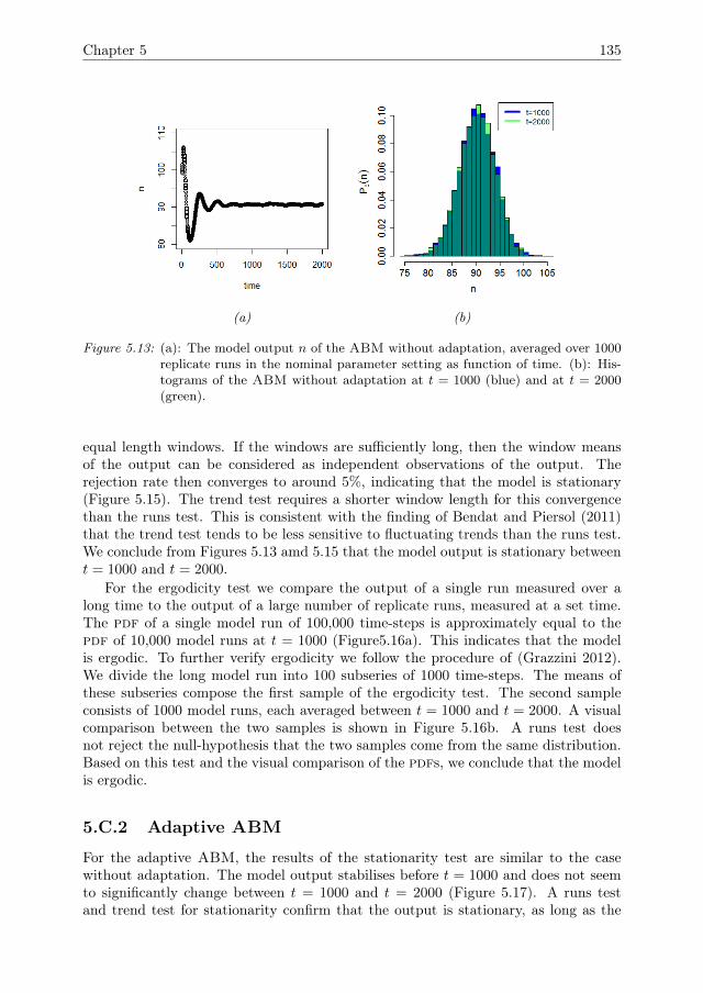
Chapter 5 135
(a) (b)
Figure 5.13: (a): The model output n of the ABM without adaptation, averaged over 1000replicate runs in the nominal parameter setting as function of time. (b): His-tograms of the ABM without adaptation at t = 1000 (blue) and at t = 2000(green).
equal length windows. If the windows are sufficiently long, then the window meansof the output can be considered as independent observations of the output. Therejection rate then converges to around 5%, indicating that the model is stationary(Figure 5.15). The trend test requires a shorter window length for this convergencethan the runs test. This is consistent with the finding of Bendat and Piersol (2011)that the trend test tends to be less sensitive to fluctuating trends than the runs test.We conclude from Figures 5.13 amd 5.15 that the model output is stationary betweent = 1000 and t = 2000.
For the ergodicity test we compare the output of a single run measured over along time to the output of a large number of replicate runs, measured at a set time.The pdf of a single model run of 100,000 time-steps is approximately equal to thepdf of 10,000 model runs at t = 1000 (Figure5.16a). This indicates that the modelis ergodic. To further verify ergodicity we follow the procedure of (Grazzini 2012).We divide the long model run into 100 subseries of 1000 time-steps. The means ofthese subseries compose the first sample of the ergodicity test. The second sampleconsists of 1000 model runs, each averaged between t = 1000 and t = 2000. A visualcomparison between the two samples is shown in Figure 5.16b. A runs test doesnot reject the null-hypothesis that the two samples come from the same distribution.Based on this test and the visual comparison of the pdfs, we conclude that the modelis ergodic.
5.C.2 Adaptive ABM
For the adaptive ABM, the results of the stationarity test are similar to the casewithout adaptation. The model output stabilises before t = 1000 and does not seemto significantly change between t = 1000 and t = 2000 (Figure 5.17). A runs testand trend test for stationarity confirm that the output is stationary, as long as the
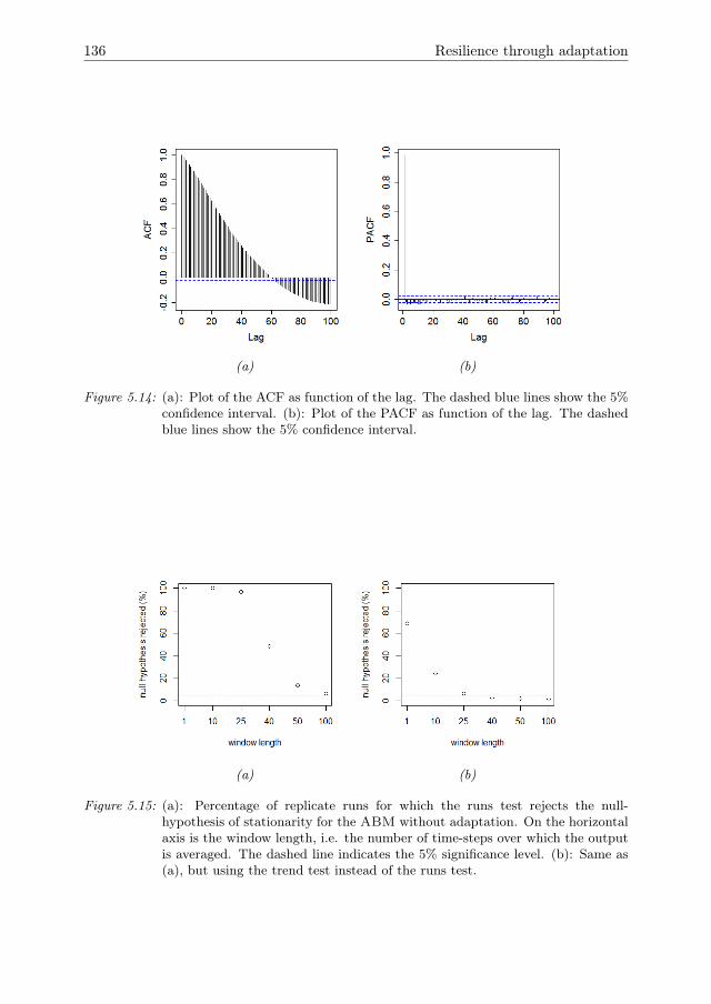
136 Resilience through adaptation
(a) (b)
Figure 5.14: (a): Plot of the ACF as function of the lag. The dashed blue lines show the 5%confidence interval. (b): Plot of the PACF as function of the lag. The dashedblue lines show the 5% confidence interval.
(a) (b)
Figure 5.15: (a): Percentage of replicate runs for which the runs test rejects the null-hypothesis of stationarity for the ABM without adaptation. On the horizontalaxis is the window length, i.e. the number of time-steps over which the outputis averaged. The dashed line indicates the 5% significance level. (b): Same as(a), but using the trend test instead of the runs test.
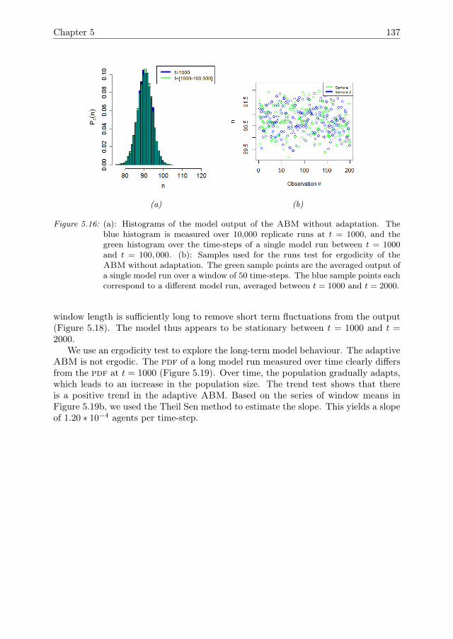
Chapter 5 137
(a) (b)
Figure 5.16: (a): Histograms of the model output of the ABM without adaptation. Theblue histogram is measured over 10,000 replicate runs at t = 1000, and thegreen histogram over the time-steps of a single model run between t = 1000and t = 100, 000. (b): Samples used for the runs test for ergodicity of theABM without adaptation. The green sample points are the averaged output ofa single model run over a window of 50 time-steps. The blue sample points eachcorrespond to a different model run, averaged between t = 1000 and t = 2000.
window length is sufficiently long to remove short term fluctuations from the output(Figure 5.18). The model thus appears to be stationary between t = 1000 and t =2000.
We use an ergodicity test to explore the long-term model behaviour. The adaptiveABM is not ergodic. The pdf of a long model run measured over time clearly differsfrom the pdf at t = 1000 (Figure 5.19). Over time, the population gradually adapts,which leads to an increase in the population size. The trend test shows that thereis a positive trend in the adaptive ABM. Based on the series of window means inFigure 5.19b, we used the Theil Sen method to estimate the slope. This yields a slopeof 1.20 ∗ 10−4 agents per time-step.
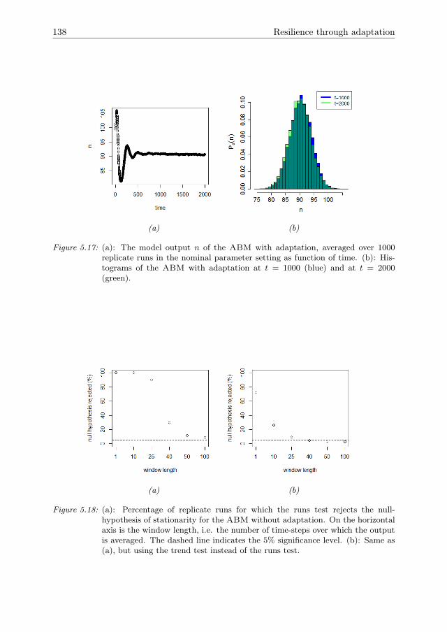
138 Resilience through adaptation
(a) (b)
Figure 5.17: (a): The model output n of the ABM with adaptation, averaged over 1000replicate runs in the nominal parameter setting as function of time. (b): His-tograms of the ABM with adaptation at t = 1000 (blue) and at t = 2000(green).
(a) (b)
Figure 5.18: (a): Percentage of replicate runs for which the runs test rejects the null-hypothesis of stationarity for the ABM without adaptation. On the horizontalaxis is the window length, i.e. the number of time-steps over which the outputis averaged. The dashed line indicates the 5% significance level. (b): Same as(a), but using the trend test instead of the runs test.
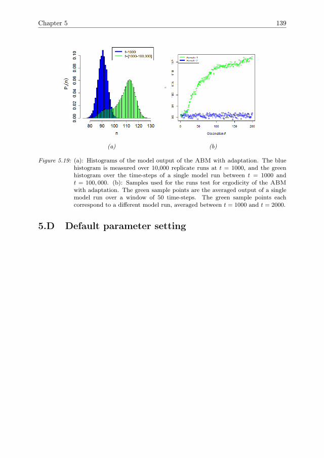
Chapter 5 139
(a) (b)
Figure 5.19: (a): Histograms of the model output of the ABM with adaptation. The bluehistogram is measured over 10,000 replicate runs at t = 1000, and the greenhistogram over the time-steps of a single model run between t = 1000 andt = 100, 000. (b): Samples used for the runs test for ergodicity of the ABMwith adaptation. The green sample points are the averaged output of a singlemodel run over a window of 50 time-steps. The green sample points eachcorrespond to a different model run, averaged between t = 1000 and t = 2000.
5.D Default parameter setting

140 Resilience through adaptation
Table 5.3: Default setting of model parameters
Symbol Description Dimensions/range Default valuec Efficiency J kg−1 0.9D Diffusion coefficient km2day−1 0.1Eb Birth energy J 5Eh Harvest cost J 0.3Em Cost of energy maintenance J 0.1Emove Move cost J 0.5K Carrying capacity kg 2n0 Initial number of agents 0,1,2, ... 100r Growth rate s−1 0.1R0 Initial resource 0-1 (proportion of K) 1Rmax Maximum harvest kg 0.5Runc Uncertainty of resource estimations kg 0.1vb Birth coefficient J−1 10vd Mortality coefficient J−1 10z Variation in offspring traits [0,→〉 0.2

Chapter 6
Cooperation can improve theresilience of common-poolresource systems againstover-harvesting
G.A. ten Broeke, G.A.K. van Voorn, A. Ligtenberg, J. Molenaar.Under review.
142 Cooperation can improve resilience
Currently common-pool resource systems world-wide are under pressure due tooverexploitation and environmental change. To ensure that these systems continueto provide vital ecosystem services it may be necessary to increase their resilienceagainst such pressure. One way of doing this may be to improve cooperation amongagents who are heavily involved in common-pool resource systems, such as farmers,fishers, managers, and companies. Historical examples suggest that the persistenceor collapse of common-pool resource systems may hinge on agents collaborating ornot, but cooperation as a mechanism to improve resilience is not commonly includedin existing models for studying resilience. Cooperation may be sustained throughindirect reciprocity, i.e., cooperative behaviour by one agent may be repaid by otheragents. In this paper we develop a suite of models to understand how cooperationcan evolve, and how it affects the resilience of common-pool resource systems.This suite of models contains various mechanisms for indirect reciprocity. Thesemechanism are modelled as agent-based models (ABMs), which represent a genericspatial common-pool resource system. The results show that although indirectreciprocity positively affects the level of cooperation in the system, cooperation iscommon even without indirect reciprocity. Moreover, the presence of cooperationincreases the resilience of the system against shocks that make it more difficult togather resource. This resilience is assessed by applying various shocks in the formof changes to state variable or parameter values, and measuring whether the agentpopulation can recover from these shocks, and how much time is needed for thisrecovery.
6.1 IntroductionThe continuing increase in the world population and its associated increase in humanactivity and environmental effects puts severe pressure on many social-ecological sys-tems (SES) (Cabell and Oelofse 2012). A particular risk seems to be a sudden loss ofecosystem services delivered by these SES through a breakdown in resilience followedby random shocks, for example, a climate event or large price fluctuation (Schefferet al. 2012). Resilience is then defined as “the capacity of a system to absorb dis-turbance and reorganize while undergoing change so as to still retain essentially thesame function, structure, identity, and feedbacks” (Walker et al. 2004); in this con-text esilience is the ability of SES to absorb shocks while maintaining the provision ofecosystem services (Folke et al. 2010). This resilience depends not only on biophysicalfactors, but also on social factors (Janssen 2015). Many SES, suh as fisheries (Ba-surto et al. 2013), irrigation systems (Cifdaloz et al. 2010), and grasslands (Crépinand Lindahl 2009), involve common-pool resources that are shared between multipleactors. In such common-pool resource systems, social norms and cooperation betweenactors may be important factors for the management of the resources (Janssen 2015,Ostrom et al. 1999, Ostrom 2015, Libre et al. 2015).
In economic theory, interactions between individuals in common-pool resourcesystems are commonly studied using game theory dilemmas, such as the well-knownprisoner’s dilemma (Kreps et al. 1982, Mao et al. 2017). These studies predict thatunder the assumption of economic rationality, individuals will over-exploit a resourceto maximise their short-term personal profits. Eventually such over-exploitation will
Chapter 6 143
lead to a collapse of the system. This outcome is commonly known as the tragedy ofthe commons (Hardin 2009, Milinski et al. 2002). One well-known example of this isthe collapse of the North-Atlantic cod fishery due to over-harvesting (Milich 1999).
Historical examples as well as more current studies suggest that cooperation maybe an important mechanism through which a tragedy of the commons may be avoided,and the resilience of common-pool resource systems may be promoted (Ostrom et al.1999). For example, in grasslands, which often are owned by several farmers, coopera-tion between farmers may be needed to avoid degradation due to over-grazing (Crépinand Lindahl 2009). Another example is the Dutch water control system, which hasbeen developed and maintained through cooperation between large numbers of ac-tors (Kaijser 2002). Yet, it has also been reported that under some circumstancescooperation may lead to such an efficient exploitation of resources, that it may causeover-harvesting (Crépin and Lindahl 2009). High levels of cooperation may lead tomore efficient harvesting and an increased population size, which in turn may putpressure on resource availability. These kinds of feedbacks are especially importantfor common-pool resource problems, in which the collective actions of agents canchange the entire system, for example through the creation of pollution, or the de-pletion of a finite resource (Gotts et al. 2003). Thus, whereas cooperation appears tobe an important factor in the resilience of common-pool resource systems, its effectsmay be subtle and context-dependent. More cooperation will not always lead to ahigher resilience.
In this paper we aim to study the effects of cooperation between agents on theresilience of common-pools resource systems against random shocks against a back-ground of increased harvesting. In order to do so, we introduce a suite of models. Inthese models agents may harvest resource individually or cooperatively. The incen-tive to cooperate rather than defect is given by indirect reciprocity, which is based onreputation (Nowak and Sigmund 1998, Nowak 2006). An individual that cooperateswill gain a good reputation, and in turn receive cooperation from others. Interactingagents however can also defect. Defection directly increases the gain for an agent atthe cost of the other individual, but it also means that the reputation of the defectingagent may decrease, incurring a future cost.
A common way of modelling trade-off dynamics between direct benefits and indi-rect costs is by using game theory models. These models typically assume a constantpopulation size and play out until some steady state value is obtained (Doebeli andHauert 2005). The main assumption in game theory models is that agents are capa-ble of decisions based on ‘perfect’ information and decision-making, i.e. they knowexactly what options exist and what the expected costs and benefits associated witheach of these options are because they are pre-defined (so-called ‘utility’ functions).This assumption may hold under certain conditions, but agents involved in manySES have limited information available and are subject to social rules and behaviour‘outside’ economic rational theory. This is the case for instance in fisheries, a typ-ical example of common-pool resource systems, where social norms affect decisionssurrounding fishing and when to exit the fishery business (Libre et al. 2015). It isincreasingly argued that social behaviour of agents should be considered when mod-elling SES (Schlueter et al. 2012). Hence, in this paper we use Agent-based Models(ABMs). These models are composed of autonomous agents that have behaviouralrules for interacting with each other and their environment. In addition, these be-
144 Cooperation can improve resilience
havioural rules may change over time as agents learn from previous experiences. Themodels also include dynamic interactions between the resource and the agents.
The remainder of the paper is set up as follows. Section 6.2 provides an overviewof the models. In our ABMs the costs and rewards depend on resource availability.Several mechanisms for cooperation are distinguished between the models, namelyreputation may 1/ influence the decision of which individuals to interact with, 2/influence the decision of whether to accept an interaction or harvest individually, or3/ influence the decision of whether to defect or cooperate. In Section 6.3 we discussthe output measures that are collected from the model, and the methodologies thatare used to analyse the model results. For the analysis of the ABM results we will usemethodologies of sensitivity analysis to assess the resilience of the population againstextinction (Ten Broeke, Van Voorn and Ligtenberg 2016). Section 6.4 contains theresults of this analysis. In Section 6.5 we conclude with the discussion.
6.2 Model Description
To assess the effects of cooperation, we will use five different versions of an ABM inwhich alternative mechanisms for cooperation are implemented. A full descriptionof the model mechanisms is given in the ODD format (Grimm et al. 2006, 2010)provided in 6.A. Here a summary is given, while the agent decision rules regardingcooperation and defection are discussed in more detail.
In the different model versions agents may harvest the common-pool resourceeither cooperatively, or individually. By harvesting cooperatively, agents may gain ahigher yield. Different model version contain different mechanisms that can lead tocooperation. These mechanisms are shown in Fig. 6.1 (adapted from (Ostrom andWalker 2004)). Central to all of these mechanisms is trust between agents. Trust isthen based on two factors, namely reputation and the memory of agents of previousinteractions. Cooperation carries a risk, because interaction partners have the optionto ‘defect’. Defection gives a higher yield for the defector, at the cost of its interactionpartner. In absence of any mechanisms to promote cooperation, selfish agents wouldmaximise their profits by always defecting. The reputation of an agent is based onall its previous interactions. Agents that often cooperate will gain a good reputation,whereas agents that often defect will gain a bad reputation.
The five model versions used in the study are:
1. The basic model. It does not contain any mechanism to promote cooperation.Although agents have the option to cooperate, there is no incentive to do so. Weuse the basic model as a benchmark for comparison to the other model versions.
2. The reciprocity model. It is based on reciprocity. Agents tend to reciprocateprevious behaviour of interaction partners. If an interaction partner is trusted, itis inferred that the partner gained this trust by cooperating in the past. There-fore, trusted agents are more likely to receive cooperation in return, whereasuntrusted agents are more likely to suffer defection.
3. The partner choice model. Agents consider trust in their choice of which otheragents to interact with. Trusted interaction partners are preferred over un-
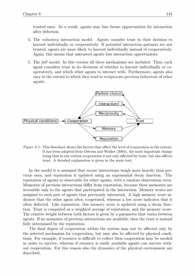
Chapter 6 145
trusted ones. As a result, agents may lose future opportunities for interactionafter defection.
4. The voluntary interaction model. Agents consider trust in their decision toharvest individually or cooperatively. If potential interaction partners are nottrusted, agents are more likely to harvest individually instead of cooperatively.Again, this means that untrusted agents lose interaction opportunities.
5. The full model. In this version all three mechanisms are included. Thus, eachagent considers trust in its decisions of whether to harvest individually or co-operatively, and which other agents to interact with. Furthermore, agents alsovary in the extend to which they tend to reciprocate previous behaviour of otheragents.
Figure 6.1: This flowchart shows the factors that affect the level of cooperation in the system.It has been adapted from Ostrom and Walker (2004), the most important changebeing that in our version cooperation is not only affected by trust, but also affectstrust. A detailed explanation is given in the main text.
In the model it is assumed that recent interactions weigh more heavily than pre-vious ones, and reputation is updated using an exponential decay function. Thereputation of agents is observable for other agents, with a random observation error.Memories of previous interactions differ from reputation, because these memories areaccessible only to the agents that participated in the interaction. Memory scores areassigned to each pair of agents that previously interacted. A high memory score in-dicates that the other agent often cooperated, whereas a low score indicates that itoften defected. Like reputation, this memory score is updated using a decay func-tion. Trust is computed as a weighted average of reputation, and the memory score.The relative weight between both factors is given by a parameter that varies betweenagents. If no memories of previous interactions are available, then the trust is insteadfully determined by the reputation.
The final degree of cooperation within the system may not be affected only bythe selected mechanism for cooperation, but amy also be affected by physical condi-tions. For example, if resource is difficult to collect then cooperation may be neededin order to survive, whereas if resource is easily available agents can survive with-out cooperation. For this reason also the dynamics of the physical environment aredescribed.
146 Cooperation can improve resilience
The agents live in a spatial environment, which is composed of a square gridof patches. Resource grows on these patches following a logistic growth equation,and diffuses between patches. Agents can move between and harvest from patches.All agent decisions are stochastic. The probabilities that govern decision-making aredetermined by the state of the agent (e.g., whether it is ‘hungry’), and the state of thesurroundings (e.g., availability of resource, presence of other agents). All agent actionscost energy, which is replenished by harvesting resource. When an agent chooses toharvest, it may do so individually or in cooperation with a neighbouring agent. Anindividual harvester takes resource from its own patch only. Cooperating harvesterstake resource from the two involved patches, and share this resource equally. Energycosts for harvesting are proportional to the amount of resource harvested, but the costis higher for individual harvesters than for cooperating harvesters. Defecting agentsdo not invest in harvesting their own patch and thus does not take any resource fromits patch; instead, they claim half of the total harvest. Defection gives a high netyield for a defector, at the cost of the yield of its interaction partner.
In terms of studying resilience it is relevant to also consider the possibilities ofagents changing their behaviour, which may result in changes in the ‘social’ resilienceof SES. In the model it is assumed that agents can change their behaviour in twoways, namely due to learning and due to adaptation. Learning typically takes placeon shorter time-scales, and is based on the memories that individual agents have ofprevious interactions. Agents may learn to cooperate with agents that cooperatedin previous interactions. Adaptation occurs through natural selection that operateson the agent population level, and typically works through a hereditary mechanismthat take place on longer time-scales. This mechanism was considered earlier byTen Broeke et al. (2017). The values of hereditary parameters remain constant overthe lifetime of an individual agent, although there is diversity in the values they havefor different agents. When new agents are born, they ‘inherit’ the parameter valuesof their parents with some random deviation. As not all agents are equally successful,bias in parameter distributions may appear over time, i.e. evolution occurs. Heredi-tary parameters in the model are waharvest and w
amove, which affect the probabilities
to harvest or move of agent a. The parameter warep represents the relative weightof reputation versus memory in computing trust values. The parameter wadefect canmake an agent more likely to defect rather than cooperate, or vice versa. Finally, theparameter wareciprocity determines whether the agent is likely to reciprocate previousbehaviour of its interaction partner when deciding on whether to defect or cooperate.
6.3 Model analysis methodology
6.3.1 Output measures
In ABMs data is generated not only on the system-level, but also on the level of agentsand patches. A single model run generates very large amounts of data. To gain agood understanding of model behaviour, proper output measures need to be selected.Basic system-level output measures are the total population size n(t), and the totalamount of resource
∑Ri,j . These measures reveal how efficient the agent population
is at gathering resource, and to what extent the resource is (over-)exploited. Sincethe model is composed of locally interacting agents, additional measures, both on the

Chapter 6 147
agent-level and on the system-level, are needed to understand the model behaviour.In the following subsections we discuss other output measures that will be used aspart of the analysis.
Level of cooperation
Two measures will be used to assess the level of cooperation in the system. Firstly,we consider the proportion of interactions that lead to cooperation
ncoop(t)/nint(t). (6.1)
This measure may give a good indication of the level of cooperation in the system, butnormalising based on the total number of interactions can give misleading outcomesespecially if this number is very small. For example, a very small number of cooper-ations could look like a high level of cooperation if the total number of interactionsis comparatively small. We therefore use a second measure
ncoop(t)/n(t), (6.2)
with n(t) the total population size. Normalising with respect to n(t) prevents mis-leading outcomes if the number of interactions is small, but gives no information onthe number of defections relative to the number of cooperative interactions. We willtherefore use both measures complementary.
To gain insight into how agent behaviour develops we record all hereditary pa-rameters, namely waharvest, w
amove, warep, wadefect, and wareciprocity. Histograms of
these parameters will be recorded for each time-step.
Clustering measure
All interactions between agents are based on spatial proximity. As part of modelanalysis we therefore want to measure not only the size of the agent population, butalso its spatial distribution. To this end we will use the following measure for spatialclustering of agents,
γ(t) =L2
n(t)− 1
n(t)∑a=1
na<nn>(t)
5(6.3)
with n(t) the total number of agents at time t, and L2 the total number of sites onthe square field. The sum runs over all agents and na<nn>(t) denotes the number ofagents on the same patch as agent a, or one of the four neighbouring patches. Notethat Table 6.1 lists all the used symbols in the main text. Eq. 6.3 measures the meandensity of agents on the same or neighbouring patches as other agents, divided bythe mean density of agents across all patches. The mean density of agents on thesame and neighbouring patches is given by the sum in Eq. 6.3. The mean density ofagents across all patches is calculated as (n(t) − 1)L−2. A value of γ(t) = 1 meansthat both densities are equal, i.e. there is no spatial clustering. A value larger than 1
148 Cooperation can improve resilience
means that agents tend to be located at patches with more neighbouring agents thanaverage. A value smaller than 1 means that agents tend to be located at patches withfewer neighbouring agents than average.
6.3.2 Resilience
The main aim of this paper is to analyse the effect of cooperation on resilience. Itis not straightforward to specify resilience, since many definitions are in use (Grimmand Wissel 1997, Brand and Jax 2007, Folke et al. 2010). We distinguish here betweenresilience to changes in the model hereditary parameters and resilience to shocks, i.e.resilience in terms of long-term and short-term time-scales respectively.
Resilience to parameter changes
The resilience of the population also depends on biophysical parameters. In partic-ular, the carrying capacity K represents the maximal amount of resource that canbe present on a site. The analysis of an earlier version of the basic model versionwithout cooperation shows that a number of tipping points exist where the popula-tion collapses (Ten Broeke, Van Voorn and Ligtenberg 2016), i.e. if the value of K isdecreased, the available resource may become insufficient to support a stable popu-lation of agents. The presence of a hereditary mechanism that allows for adaptationimproves the resilience against such tipping points (Ten Broeke et al. 2017). Here wewill analyse whether these tipping points are affected by the presence of cooperation.For quantification, we will measure the location of tipping points in parameter spaceand then verify whether this location is affected by the presence of cooperation bycomparing the base model to model versions with mechanisms for cooperation.
Resilience to shocks
Resilience is not only relevant regarding long-term time-scales, but also in terms ofshocks with a short-term time-scale, as adaptation through hereditary mechanisms isnot fast enough to operate on shocks. The measure for resilience to shocks is basedon return time (Gunderson 2000). First, the model is run for a large number of time-steps until the output has stabilised. Note that, due to stochasticity, the model outputwill always show fluctuations after this stabilisation. Once the model has stabilised ashock is introduced. The strength of the shock is measured as the sudden decrease inresource Ri,j(t) on all sites i, j. Alternatively, a shock can be a temporary change inr (the resource growth rate) or Rmax (the maximum harvest size), the latter whichrepresents a higher difficulty for agents to gather resource. The effects on the variousoutput measures are recorded, specifically
• the decrease in population size caused by the shock (this can be complete ex-tinction of the population), and
• the time required for the population to recover from the shock.
The decrease in population size caused by the shock (i.e., the effect of the shock)is quantified by measuring the difference between population size at the time of theshock and its minimum value before the population starts to recover
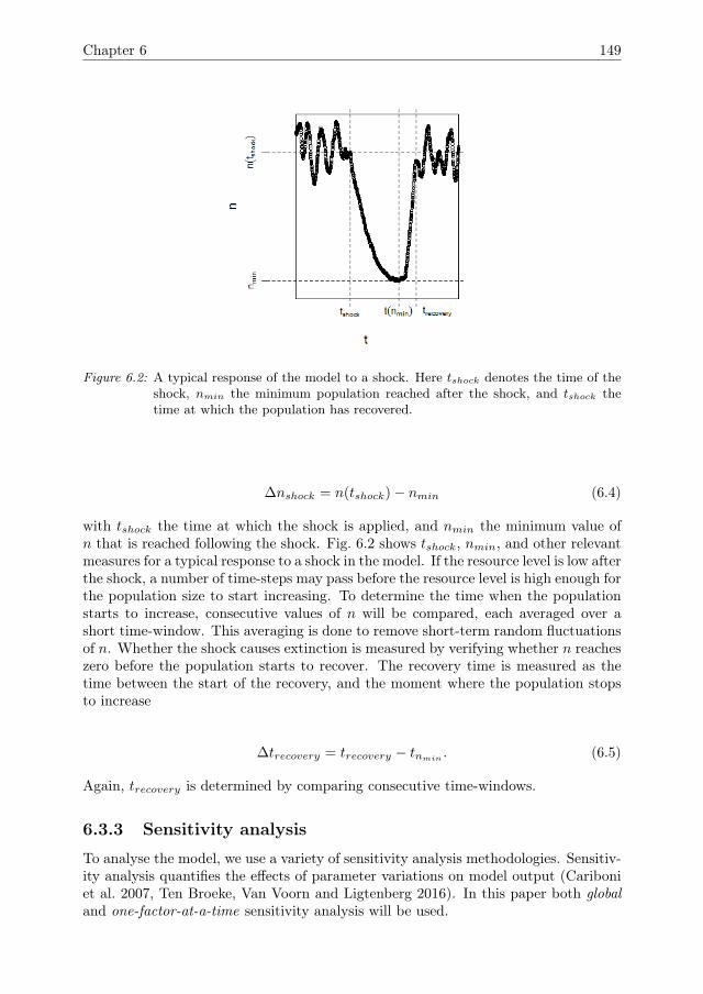
Chapter 6 149
Figure 6.2: A typical response of the model to a shock. Here tshock denotes the time of theshock, nmin the minimum population reached after the shock, and tshock thetime at which the population has recovered.
∆nshock = n(tshock)− nmin (6.4)
with tshock the time at which the shock is applied, and nmin the minimum value ofn that is reached following the shock. Fig. 6.2 shows tshock, nmin, and other relevantmeasures for a typical response to a shock in the model. If the resource level is low afterthe shock, a number of time-steps may pass before the resource level is high enough forthe population size to start increasing. To determine the time when the populationstarts to increase, consecutive values of n will be compared, each averaged over ashort time-window. This averaging is done to remove short-term random fluctuationsof n. Whether the shock causes extinction is measured by verifying whether n reacheszero before the population starts to recover. The recovery time is measured as thetime between the start of the recovery, and the moment where the population stopsto increase
∆trecovery = trecovery − tnmin. (6.5)
Again, trecovery is determined by comparing consecutive time-windows.
6.3.3 Sensitivity analysis
To analyse the model, we use a variety of sensitivity analysis methodologies. Sensitiv-ity analysis quantifies the effects of parameter variations on model output (Cariboniet al. 2007, Ten Broeke, Van Voorn and Ligtenberg 2016). In this paper both globaland one-factor-at-a-time sensitivity analysis will be used.

150 Cooperation can improve resilience
Global sensitivity analysis
In global sensitivity analysis all parameters are varied simultaneously across a regionof parameter space (Cariboni et al. 2007). The variation of the model output acrossthis range is quantified by calculating the variance and decomposed the variance intoterms that are attributed to the various model parameters (i.e., conditional variances).The model parameters can then be ranked based on how strongly they influencethe model output. Since parameters are varied simultaneously interaction effectsmay be taken into account. However, aggregating the model output across a regionof parameter space makes it difficult to infer causal relationships between specificparameters and model outputs (Ten Broeke, Van Voorn and Ligtenberg 2016). Wetherefore supplement global sensitivity analysis with one-factor-at-a-time sensitivityanalysis.
One-factor-at-a-time sensitivity analysis (OFAT)
OFAT examines the effect of an individual parameter on the model output whilekeeping the other parameter values constant. Model outputs are plotted as a functionof the varied parameter. The main advantage of OFAT is that it shows clearly therelationship between individual parameters and the model output, including whetherthis relationship is linear or non-linear. Furthermore, OFAT is a better tool fordetecting tipping points than global sensitivity measures (Ten Broeke, Van Voornand Ligtenberg 2016, Ten Broeke et al. 2017).
Table 6.1: List of used symbols.
Symbol Description Units/rangea Index for agents 0,1,2, ...i, j Indices for patches [1, L]K Carrying capacity massL Lattice size distancen(t) Number of agents 0,1,2, . . .na<nn>(t) Number of nearest neighbours for agent a 0,1,2, . . .ncoop(t) Number of cooperations 0,1,2, . . .nint(t) Number of interactions 0,1,2, . . .r Resource growth rate time−1
Rij(t) Resource at patch i, j at time t massRmax Maximum harvest size massRshock Resource level after shock masst Time timewadefect Parameter representing probability to defect [0, 1]
waharvest Harvest coefficient [0,→〉wamove Move coefficient [0,→〉wareciprocity Weight assigned to reciprocity in interactions [0, 1]warep Weight assigned to reputation in interactions [0, 1]z Variation in offspring traits [0, 1]γ(t) Clustering measure [0,→〉
Chapter 6 151
6.4 Results
6.4.1 Default parameter setting
For benchmarking the different model versions are first studied at default parametersettings. In the full model version, which contains all mechanisms for cooperation, astable high level of cooperation is maintained (Fig. 6.3), while the trajectories of theagent parameters are also stable, as is shown for wdefect in Fig. 6.3.
In Fig. 6.4a it can be seen that any mechanism promoting cooperation leads tomore or less the same (high) level of n(t), whereas absence of such a mechanism givesrise to very low values of n(t). Lack of a mechanism to support cooperation makesthe population as a whole less efficient in using the available resources. The decreasedpopulation size is accompanied by a decrease in the level of cooperation between agents(Fig. 6.4b). In the base model (black), around 40% of interactions end in cooperation,and the remaining interactions lead to defection. In the reciprocity model (blue) andthe partner choice model (green) the level of cooperation is clearly higher than inthe base model. In the voluntary interaction model (red), the level of cooperationis lower, but the total number of interactions is also much lower (Fig. 6.4c). Thus,even though most interactions end in defection, the number of defections is lowerthan in the base model. These results suggest that cooperation is better promotedby mechanisms other than a mechanism for voluntary cooperation.
Even though mechanisms for reciprocity positively affect the level of cooperation,the finding that cooperation in the base model is common even without reciprocitymay seem surprising. In absence of any mechanism to support cooperation, it might beexpected that agents would never cooperate. Yet the results in Fig. 6.4b,c show thatcooperation in the base model is common. To understand this finding, note that thebase model shows a strong degree of spatial clustering of agents. For example, Fig. 6.5shows a typical spatial arrangement of agents in the base model. Fig. 6.6 shows theamount of clustering as function of time for each of the model versions. Clearly spatialclustering is very strong in the base model, whereas the other model versions showlittle clustering on long time-scales. The presence of these clusters leads to an increasein the level of cooperation. Clusters with high defection rates disappear quicklyfrom the simulation, because defections hinder the survival of interaction partners.Clusters with a high level of cooperation, in contrast, can survive for extended periods.However, such clusters are susceptible to exploitation by agents that defect often.This susceptibility limits the growth of these clusters. As a result, some regions ofthe lattice remain completely empty, which explains the large difference in populationsize between the model versions (Fig. 6.4a).
6.4.2 Sensitivity analysis
The qualitative effects of cooperation on model output are evaluated using the OFATanalysis for all of the model parameters. Given the large number of parameters, welimit the discussion to only a few parameters that affect the model behaviour strongly.To further quantify the effects of cooperation sensitivity analysis is performed forboth the base and the full model. Details of the global sensitivity analysis are givenin 6.C. The main outcome of the global sensitivity analysis is that both model versionscontain tipping points where the population goes extinct. Out of 1000 sample points,
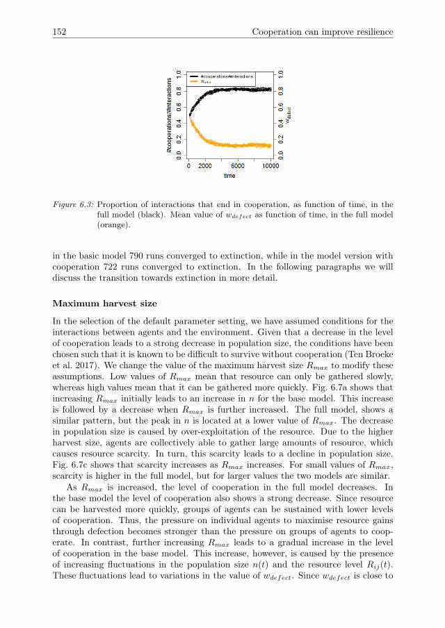
152 Cooperation can improve resilience
Figure 6.3: Proportion of interactions that end in cooperation, as function of time, in thefull model (black). Mean value of wdefect as function of time, in the full model(orange).
in the basic model 790 runs converged to extinction, while in the model version withcooperation 722 runs converged to extinction. In the following paragraphs we willdiscuss the transition towards extinction in more detail.
Maximum harvest size
In the selection of the default parameter setting, we have assumed conditions for theinteractions between agents and the environment. Given that a decrease in the levelof cooperation leads to a strong decrease in population size, the conditions have beenchosen such that it is known to be difficult to survive without cooperation (Ten Broekeet al. 2017). We change the value of the maximum harvest size Rmax to modify theseassumptions. Low values of Rmax mean that resource can only be gathered slowly,whereas high values mean that it can be gathered more quickly. Fig. 6.7a shows thatincreasing Rmax initially leads to an increase in n for the base model. This increaseis followed by a decrease when Rmax is further increased. The full model, shows asimilar pattern, but the peak in n is located at a lower value of Rmax. The decreasein population size is caused by over-exploitation of the resource. Due to the higherharvest size, agents are collectively able to gather large amounts of resource, whichcauses resource scarcity. In turn, this scarcity leads to a decline in population size.Fig. 6.7c shows that scarcity increases as Rmax increases. For small values of Rmax,scarcity is higher in the full model, but for larger values the two models are similar.
As Rmax is increased, the level of cooperation in the full model decreases. Inthe base model the level of cooperation also shows a strong decrease. Since resourcecan be harvested more quickly, groups of agents can be sustained with lower levelsof cooperation. Thus, the pressure on individual agents to maximise resource gainsthrough defection becomes stronger than the pressure on groups of agents to coop-erate. In contrast, further increasing Rmax leads to a gradual increase in the levelof cooperation in the base model. This increase, however, is caused by the presenceof increasing fluctuations in the population size n(t) and the resource level Rij(t).These fluctuations lead to variations in the value of wdefect. Since wdefect is close to
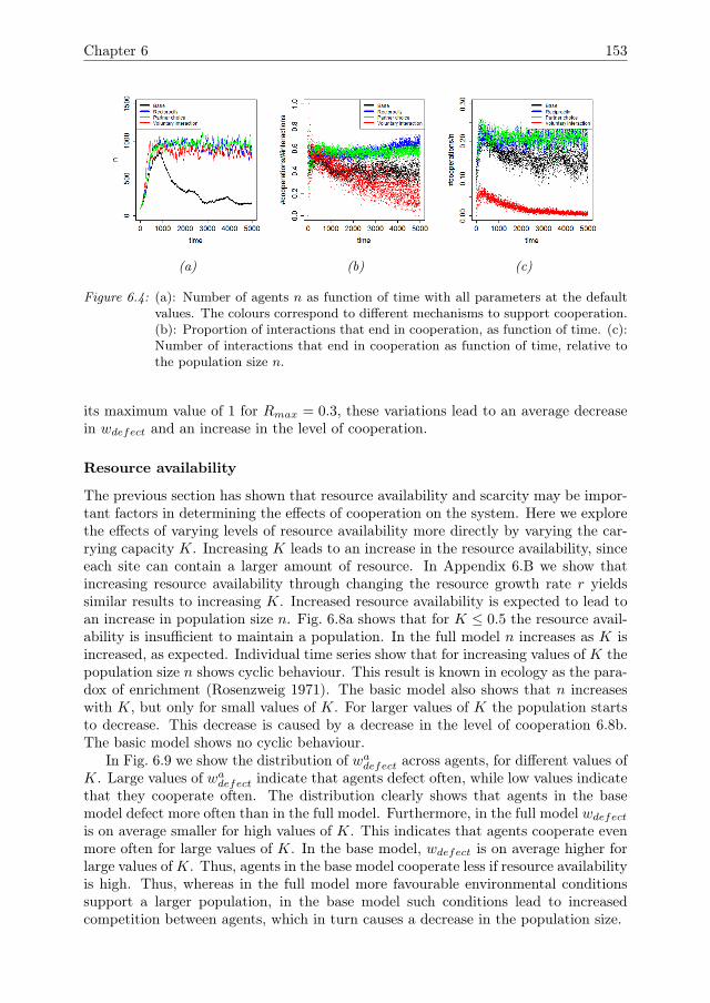
Chapter 6 153
(a) (b) (c)
Figure 6.4: (a): Number of agents n as function of time with all parameters at the defaultvalues. The colours correspond to different mechanisms to support cooperation.(b): Proportion of interactions that end in cooperation, as function of time. (c):Number of interactions that end in cooperation as function of time, relative tothe population size n.
its maximum value of 1 for Rmax = 0.3, these variations lead to an average decreasein wdefect and an increase in the level of cooperation.
Resource availability
The previous section has shown that resource availability and scarcity may be impor-tant factors in determining the effects of cooperation on the system. Here we explorethe effects of varying levels of resource availability more directly by varying the car-rying capacity K. Increasing K leads to an increase in the resource availability, sinceeach site can contain a larger amount of resource. In Appendix 6.B we show thatincreasing resource availability through changing the resource growth rate r yieldssimilar results to increasing K. Increased resource availability is expected to lead toan increase in population size n. Fig. 6.8a shows that for K ≤ 0.5 the resource avail-ability is insufficient to maintain a population. In the full model n increases as K isincreased, as expected. Individual time series show that for increasing values of K thepopulation size n shows cyclic behaviour. This result is known in ecology as the para-dox of enrichment (Rosenzweig 1971). The basic model also shows that n increaseswith K, but only for small values of K. For larger values of K the population startsto decrease. This decrease is caused by a decrease in the level of cooperation 6.8b.The basic model shows no cyclic behaviour.
In Fig. 6.9 we show the distribution of wadefect across agents, for different values ofK. Large values of wadefect indicate that agents defect often, while low values indicatethat they cooperate often. The distribution clearly shows that agents in the basemodel defect more often than in the full model. Furthermore, in the full model wdefectis on average smaller for high values of K. This indicates that agents cooperate evenmore often for large values of K. In the base model, wdefect is on average higher forlarge values ofK. Thus, agents in the base model cooperate less if resource availabilityis high. Thus, whereas in the full model more favourable environmental conditionssupport a larger population, in the base model such conditions lead to increasedcompetition between agents, which in turn causes a decrease in the population size.
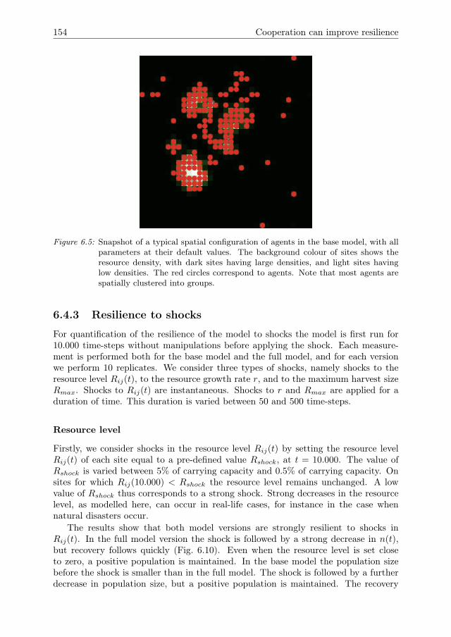
154 Cooperation can improve resilience
Figure 6.5: Snapshot of a typical spatial configuration of agents in the base model, with allparameters at their default values. The background colour of sites shows theresource density, with dark sites having large densities, and light sites havinglow densities. The red circles correspond to agents. Note that most agents arespatially clustered into groups.
6.4.3 Resilience to shocks
For quantification of the resilience of the model to shocks the model is first run for10.000 time-steps without manipulations before applying the shock. Each measure-ment is performed both for the base model and the full model, and for each versionwe perform 10 replicates. We consider three types of shocks, namely shocks to theresource level Rij(t), to the resource growth rate r, and to the maximum harvest sizeRmax. Shocks to Rij(t) are instantaneous. Shocks to r and Rmax are applied for aduration of time. This duration is varied between 50 and 500 time-steps.
Resource level
Firstly, we consider shocks in the resource level Rij(t) by setting the resource levelRij(t) of each site equal to a pre-defined value Rshock, at t = 10.000. The value ofRshock is varied between 5% of carrying capacity and 0.5% of carrying capacity. Onsites for which Rij(10.000) < Rshock the resource level remains unchanged. A lowvalue of Rshock thus corresponds to a strong shock. Strong decreases in the resourcelevel, as modelled here, can occur in real-life cases, for instance in the case whennatural disasters occur.
The results show that both model versions are strongly resilient to shocks inRij(t). In the full model version the shock is followed by a strong decrease in n(t),but recovery follows quickly (Fig. 6.10). Even when the resource level is set closeto zero, a positive population is maintained. In the base model the population sizebefore the shock is smaller than in the full model. The shock is followed by a furtherdecrease in population size, but a positive population is maintained. The recovery
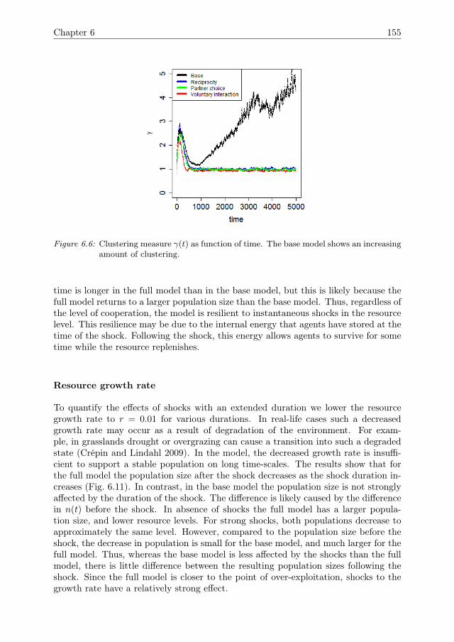
Chapter 6 155
Figure 6.6: Clustering measure γ(t) as function of time. The base model shows an increasingamount of clustering.
time is longer in the full model than in the base model, but this is likely because thefull model returns to a larger population size than the base model. Thus, regardless ofthe level of cooperation, the model is resilient to instantaneous shocks in the resourcelevel. This resilience may be due to the internal energy that agents have stored at thetime of the shock. Following the shock, this energy allows agents to survive for sometime while the resource replenishes.
Resource growth rate
To quantify the effects of shocks with an extended duration we lower the resourcegrowth rate to r = 0.01 for various durations. In real-life cases such a decreasedgrowth rate may occur as a result of degradation of the environment. For exam-ple, in grasslands drought or overgrazing can cause a transition into such a degradedstate (Crépin and Lindahl 2009). In the model, the decreased growth rate is insuffi-cient to support a stable population on long time-scales. The results show that forthe full model the population size after the shock decreases as the shock duration in-creases (Fig. 6.11). In contrast, in the base model the population size is not stronglyaffected by the duration of the shock. The difference is likely caused by the differencein n(t) before the shock. In absence of shocks the full model has a larger popula-tion size, and lower resource levels. For strong shocks, both populations decrease toapproximately the same level. However, compared to the population size before theshock, the decrease in population is small for the base model, and much larger for thefull model. Thus, whereas the base model is less affected by the shocks than the fullmodel, there is little difference between the resulting population sizes following theshock. Since the full model is closer to the point of over-exploitation, shocks to thegrowth rate have a relatively strong effect.
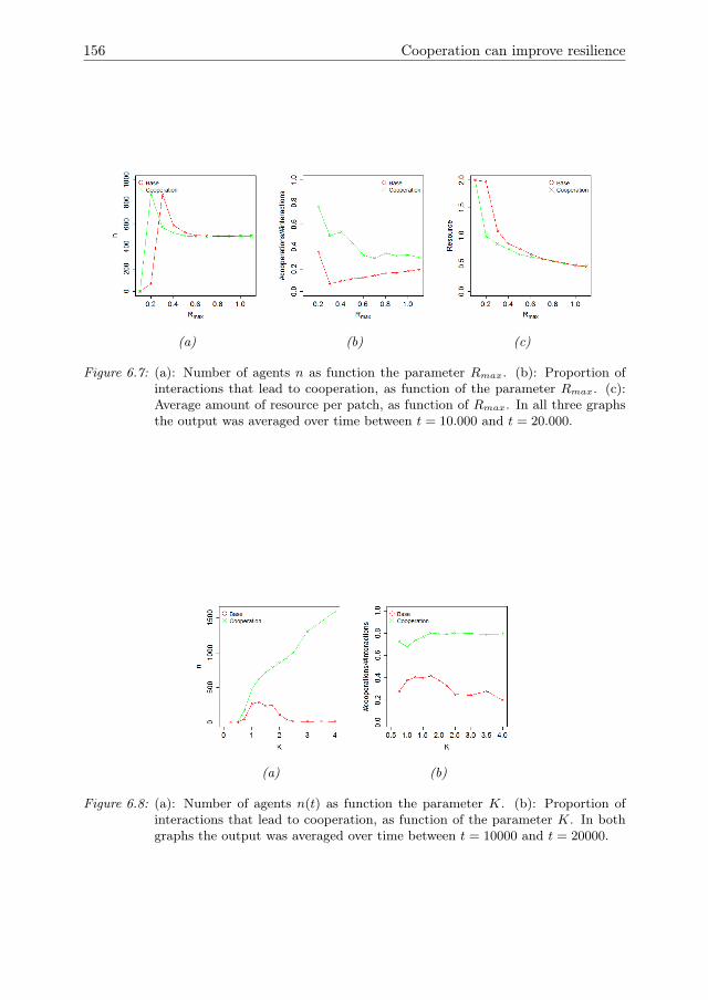
156 Cooperation can improve resilience
(a) (b) (c)
Figure 6.7: (a): Number of agents n as function the parameter Rmax. (b): Proportion ofinteractions that lead to cooperation, as function of the parameter Rmax. (c):Average amount of resource per patch, as function of Rmax. In all three graphsthe output was averaged over time between t = 10.000 and t = 20.000.
(a) (b)
Figure 6.8: (a): Number of agents n(t) as function the parameter K. (b): Proportion ofinteractions that lead to cooperation, as function of the parameter K. In bothgraphs the output was averaged over time between t = 10000 and t = 20000.
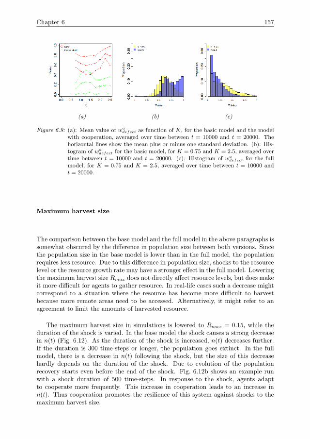
Chapter 6 157
(a) (b) (c)
Figure 6.9: (a): Mean value of wadefect as function of K, for the basic model and the modelwith cooperation, averaged over time between t = 10000 and t = 20000. Thehorizontal lines show the mean plus or minus one standard deviation. (b): His-togram of wadefect for the basic model, for K = 0.75 and K = 2.5, averaged overtime between t = 10000 and t = 20000. (c): Histogram of wadefect for the fullmodel, for K = 0.75 and K = 2.5, averaged over time between t = 10000 andt = 20000.
Maximum harvest size
The comparison between the base model and the full model in the above paragraphs issomewhat obscured by the difference in population size between both versions. Sincethe population size in the base model is lower than in the full model, the populationrequires less resource. Due to this difference in population size, shocks to the resourcelevel or the resource growth rate may have a stronger effect in the full model. Loweringthe maximum harvest size Rmax does not directly affect resource levels, but does makeit more difficult for agents to gather resource. In real-life cases such a decrease mightcorrespond to a situation where the resource has become more difficult to harvestbecause more remote areas need to be accessed. Alternatively, it might refer to anagreement to limit the amounts of harvested resource.
The maximum harvest size in simulations is lowered to Rmax = 0.15, while theduration of the shock is varied. In the base model the shock causes a strong decreasein n(t) (Fig. 6.12). As the duration of the shock is increased, n(t) decreases further.If the duration is 300 time-steps or longer, the population goes extinct. In the fullmodel, there is a decrease in n(t) following the shock, but the size of this decreasehardly depends on the duration of the shock. Due to evolution of the populationrecovery starts even before the end of the shock. Fig. 6.12b shows an example runwith a shock duration of 500 time-steps. In response to the shock, agents adaptto cooperate more frequently. This increase in cooperation leads to an increase inn(t). Thus cooperation promotes the resilience of this system against shocks to themaximum harvest size.
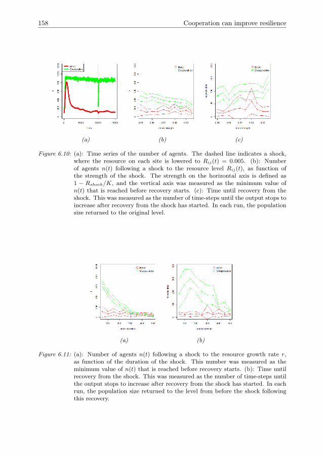
158 Cooperation can improve resilience
(a) (b) (c)
Figure 6.10: (a): Time series of the number of agents. The dashed line indicates a shock,where the resource on each site is lowered to Rij(t) = 0.005. (b): Numberof agents n(t) following a shock to the resource level Rij(t), as function ofthe strength of the shock. The strength on the horizontal axis is defined as1 − Rshock/K, and the vertical axis was measured as the minimum value ofn(t) that is reached before recovery starts. (c): Time until recovery from theshock. This was measured as the number of time-steps until the output stops toincrease after recovery from the shock has started. In each run, the populationsize returned to the original level.
(a) (b)
Figure 6.11: (a): Number of agents n(t) following a shock to the resource growth rate r,as function of the duration of the shock. This number was measured as theminimum value of n(t) that is reached before recovery starts. (b): Time untilrecovery from the shock. This was measured as the number of time-steps untilthe output stops to increase after recovery from the shock has started. In eachrun, the population size returned to the level from before the shock followingthis recovery.
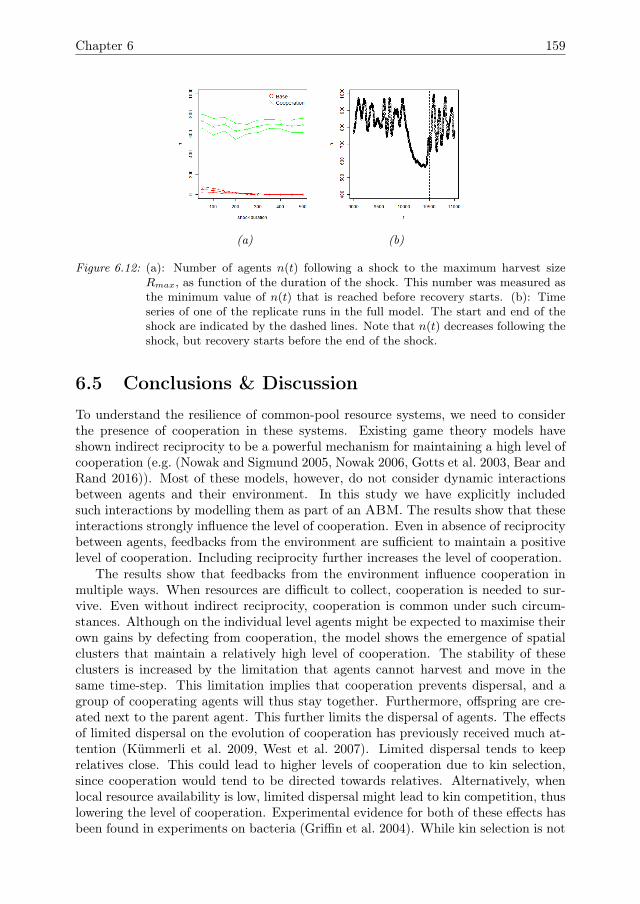
Chapter 6 159
(a) (b)
Figure 6.12: (a): Number of agents n(t) following a shock to the maximum harvest sizeRmax, as function of the duration of the shock. This number was measured asthe minimum value of n(t) that is reached before recovery starts. (b): Timeseries of one of the replicate runs in the full model. The start and end of theshock are indicated by the dashed lines. Note that n(t) decreases following theshock, but recovery starts before the end of the shock.
6.5 Conclusions & Discussion
To understand the resilience of common-pool resource systems, we need to considerthe presence of cooperation in these systems. Existing game theory models haveshown indirect reciprocity to be a powerful mechanism for maintaining a high level ofcooperation (e.g. (Nowak and Sigmund 2005, Nowak 2006, Gotts et al. 2003, Bear andRand 2016)). Most of these models, however, do not consider dynamic interactionsbetween agents and their environment. In this study we have explicitly includedsuch interactions by modelling them as part of an ABM. The results show that theseinteractions strongly influence the level of cooperation. Even in absence of reciprocitybetween agents, feedbacks from the environment are sufficient to maintain a positivelevel of cooperation. Including reciprocity further increases the level of cooperation.
The results show that feedbacks from the environment influence cooperation inmultiple ways. When resources are difficult to collect, cooperation is needed to sur-vive. Even without indirect reciprocity, cooperation is common under such circum-stances. Although on the individual level agents might be expected to maximise theirown gains by defecting from cooperation, the model shows the emergence of spatialclusters that maintain a relatively high level of cooperation. The stability of theseclusters is increased by the limitation that agents cannot harvest and move in thesame time-step. This limitation implies that cooperation prevents dispersal, and agroup of cooperating agents will thus stay together. Furthermore, offspring are cre-ated next to the parent agent. This further limits the dispersal of agents. The effectsof limited dispersal on the evolution of cooperation has previously received much at-tention (Kümmerli et al. 2009, West et al. 2007). Limited dispersal tends to keeprelatives close. This could lead to higher levels of cooperation due to kin selection,since cooperation would tend to be directed towards relatives. Alternatively, whenlocal resource availability is low, limited dispersal might lead to kin competition, thuslowering the level of cooperation. Experimental evidence for both of these effects hasbeen found in experiments on bacteria (Griffin et al. 2004). While kin selection is not

160 Cooperation can improve resilience
included in our model, it might be an interesting area for future research.
The trajectories of the agent parameters in the model appear to be stable, as isshown for wdefect in the default setting in Fig. 6.3. Each of the parameters graduallyconverges, after which it shows only small random fluctuations around a constantmean. In the full model, this convergence leads to a stable and high level of co-operation. This contrasts with results from previous studies (Nowak and Sigmund1998, Lindgren 1992). In Nowak and Sigmund (1998) it was found that periods withmany agents that tend to cooperate were interrupted by periods with many defectors.The relative stability of the agent parameters in our study may be due to adaptationthrough evolution occurring relatively slowly. This adaptation occurs slowly becauseagents on average participate in a number of interactions before creating offspring,and the differences between offspring and parents are small. Thus, for defection tospread, on average defectors need to be successful over a large number of interactions.In contrast, in Nowak and Sigmund (1998) a much lower number of interactions pergeneration was used. In our model, learning occurs on similarly short time-scales. Inthe model, if learning is more important than cooperation, the fluctuations in the levelof cooperation are larger (results not shown). This difference in time-scales over whichlearning and adaptation occur was not present in previous models of cooperation, andmay be an interesting topic for further study.
Although our results show that reciprocity is not needed to maintain a positive ofcooperation, reciprocity does further increase the level of cooperation, and increasesthe range of environmental conditions for which cooperation can evolve. The increasedlevel of cooperation leads to an increased population size. The increased level ofcooperation may affect the resilience of the system in different ways, depending onthe type of shock. Thus, to assess the resilience it is crucial to specify both the typeof shock that is applied, and the component of the system that needs to be resilient,i.e. ‘resilience of what to what’ (Carpenter et al. 2001). Systems with a higher levelof cooperation use resources more efficiently, but also may be closer to the point ofover-exploitation. As a result, shocks to the resource level can have a strong impactwhen they lead to sudden over-exploitation. Shocks to the maximum harvest sizehave little effect, because due to cooperation the agents still manage to gain sufficientenergy from the harvests. In systems with little cooperation, in contrast, competitionbetween agents makes it more difficult to obtain sufficient energy from harvests. As aresult, the population size is decreased, and the system is far from over-exploitation.Therefore, shocks to the resource level hardly have any effect, whereas shocks to themaximum harvest size quickly lead to extinction.
Our study shows that the resilience of the model depends strongly on coopera-tion. But it depends on the circumstances whether this cooperation has a positiveor a negative on the resilience. These results show that in real-life cases cooperationis a relevant factor to consider when assessing the resilience of SES. However, pre-cisely how cooperation affects the resilience may depend on the specific case. Morecooperation may lead to a higher resilience in some contexts, but in other contexts itmight lead to over-harvesting. Thus, the case-specific context should be consideredcarefully when assessing the effects of cooperation on resilience in a real-life system.
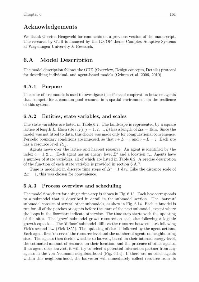
Chapter 6 161
Acknowledgements
We thank Geerten Hengeveld for comments on a previous version of the manuscript.The research by GTB is financed by the IO/OP theme Complex Adaptive Systemsat Wageningen University & Research.
6.A Model Description
The model description follows the ODD (Overview, Design concepts, Details) protocolfor describing individual- and agent-based models (Grimm et al. 2006, 2010).
6.A.1 Purpose
The suite of five models is used to investigate the effects of cooperation between agentsthat compete for a common-pool resource in a spatial environment on the resilienceof this system.
6.A.2 Entities, state variables, and scales
The state variables are listed in Table 6.2. The landscape is represented by a squarelattice of length L. Each site i, j(i, j = 1, 2, ..., L) has a length of ∆x = 1km. Since themodel was not fitted to data, this choice was made only for computational convenience.Periodic boundary conditions are imposed, so that i+L = i and j+L = j. Each sitehas a resource level Ri,j .
Agents move over the lattice and harvest resource. An agent is identified by theindex a = 1, 2, .... Each agent has an energy level Ea and a location xa. Agents havea number of state variables, all of which are listed in Table 6.2. A precise descriptionof the function of each state variable is provided in section 6.A.7.
Time is modelled in discrete time steps of ∆t = 1 day. Like the distance scale of∆x = 1, this was chosen for convenience.
6.A.3 Process overview and scheduling
The model flow chart for a single time-step is shown in Fig. 6.13. Each box correspondsto a submodel that is described in detail in the submodel section. The ‘harvest’submodel consists of several other submodels, as show in Fig. 6.14. Each submodel isrun for all of the patches or agents before the start of the next submodel, except wherethe loops in the flowchart indicate otherwise. The time-step starts with the updatingof the sites. The ‘grow’ submodel grows resource on each site following a logisticgrowth equation. The ‘diffuse’ submodel diffuses the resource between sites followingFick’s second law (Fick 1855). The updating of sites is followed by the agent actions.Each agent first ‘observes’ the resource level and the number of agents on neighbouringsites. The agents then decide whether to harvest, based on their internal energy level,the estimated amount of resource on their location, and the presence of other agents.If an agent does harvest, it will try to select a potential interaction partner from anyagents in the von Neumann neighbourhood (Fig. 6.14). If there are no other agentswithin this neighbourhood, the harvester will immediately collect resource from its

162 Cooperation can improve resilience
site. If a partner is found, then it will decide whether or not to interact with thatagent, based on the trust it has towards the agent and the available resource on thatagent’s site. If it chooses not to interact, it will proceed to collect resource fromits own site. If it chooses to interact, then the interaction partner decides whetherto defect or cooperate before resource is collected. If an agent does not harvest, itmay decide to move based on the number of agents and estimated resource level onneighbouring sites. Alternatively, an agent may decide to neither harvest nor move,thus conserving energy. After all the actions of harvesting and moving have beencarried out, each agent pays a fixed energy maintenance. There is a possibility thatan agent will then die or breed, depending on its internal energy. The model thenproceeds to the next time-step.
6.A.4 Design concepts
Basic principles
The model describes agents that move and harvest in a spatial environment. Basedon their internal state (i.e., internal energy) and the state of the environment (i.e.,available resource, presence of other agents) agents may decide to move to a new lo-cation, harvest from the present location, or wait for a better opportunity. Harvestedresource is converted to internal energy, which is used to pay for daily maintenanceand the actions of moving and harvesting. Harvesting may be done either individually,or in cooperation with an agent on a neighbouring site. When cooperating, agentsneed less energy to harvest the same amount of resource. Cooperation is thus moreefficient that harvesting individually, but it puts agents at risk of ‘defecting’ interac-tion partners. A defecting agent does not invest energy in the harvest, but still claimshalf of the resource. As a result, the net energy gain for a defecting agent is largerthan for a cooperating agent. However, defection damages the reputation of an agentand the trust it receives from other agents. In the short-term, defection will help theagent to accumulate a larger amount of resource. On the long term, however, thelowered reputation and trust may make other agents less likely to enter interactionswith the agent. Thus, although defection yields an advantage on the short term, onthe long term such behaviour might be punished.
Emergence
We consider the total population size ntot and the distribution of wah, wam, warep,
wadefect, ρa, and τa,a
′across the population as emerging variables at the macro-level.
In addition, the level of cooperation in the system is also considered emergent. Thislevel of cooperation is measured by keeping track of how often agents choose to defect,or to cooperate, and of the trust values of the agents.
Adaptation
Agents adapt their behaviour to changes in their internal state or in their environment.Agents with low levels of internal energy tend to harvest resource with a higherprobability. Agents also tend to harvest if the resource level on their site is high andthe number of other agents on the site is low. Agents consider the state of the sites
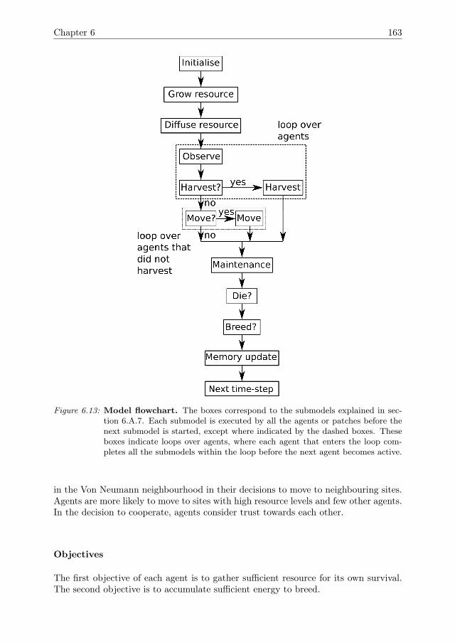
Chapter 6 163
Figure 6.13: Model flowchart. The boxes correspond to the submodels explained in sec-tion 6.A.7. Each submodel is executed by all the agents or patches before thenext submodel is started, except where indicated by the dashed boxes. Theseboxes indicate loops over agents, where each agent that enters the loop com-pletes all the submodels within the loop before the next agent becomes active.
in the Von Neumann neighbourhood in their decisions to move to neighbouring sites.Agents are more likely to move to sites with high resource levels and few other agents.In the decision to cooperate, agents consider trust towards each other.
Objectives
The first objective of each agent is to gather sufficient resource for its own survival.The second objective is to accumulate sufficient energy to breed.
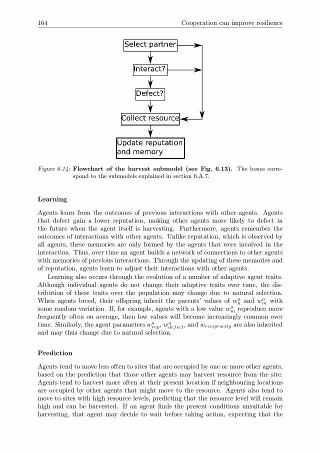
164 Cooperation can improve resilience
Figure 6.14: Flowchart of the harvest submodel (see Fig. 6.13). The boxes corre-spond to the submodels explained in section 6.A.7.
Learning
Agents learn from the outcomes of previous interactions with other agents. Agentsthat defect gain a lower reputation, making other agents more likely to defect inthe future when the agent itself is harvesting. Furthermore, agents remember theoutcomes of interactions with other agents. Unlike reputation, which is observed byall agents, these memories are only formed by the agents that were involved in theinteraction. Thus, over time an agent builds a network of connections to other agentswith memories of previous interactions. Through the updating of these memories andof reputation, agents learn to adjust their interactions with other agents.
Learning also occurs through the evolution of a number of adaptive agent traits.Although individual agents do not change their adaptive traits over time, the dis-tribution of these traits over the population may change due to natural selection.When agents breed, their offspring inherit the parents’ values of wah and wam withsome random variation. If, for example, agents with a low value wam reproduce morefrequently often on average, then low values will become increasingly common overtime. Similarly, the agent parameters warep, wadefect, and wreciprocity are also inheritedand may thus change due to natural selection.
Prediction
Agents tend to move less often to sites that are occupied by one or more other agents,based on the prediction that those other agents may harvest resource from the site.Agents tend to harvest more often at their present location if neighbouring locationsare occupied by other agents that might move to the resource. Agents also tend tomove to sites with high resource levels, predicting that the resource level will remainhigh and can be harvested. If an agent finds the present conditions unsuitable forharvesting, that agent may decide to wait before taking action, expecting that the
Chapter 6 165
conditions will improve in the future. Agents choose interaction partners with hightrust values, based on the prediction that these agents will be less likely to defect.
Sensing
Agents sense their own internal energy. Each time step, agents assess the amount ofresource on their current location and the four sites that compose the Von Neumannneighbourhood. However, agents do not sense the exact amount of resource becausethere is some random error. Agents also sense the presence of any other agents withinthe Von Neumann neighbourhood, and the reputation of those agents. There is noerror in sensing which agents are present, but there is a random error in the sensing ofthe reputation of those agents. Agents also sense their own memory of the outcomes ofprevious interactions with other agents. There is no error in sensing these memories.
Interaction
Indirect interactions between agents occur through the competition for resource. Inaddition, agents are less likely to move to sites that contain other agents. This is aform of direct interaction. Agents are also more likely to harvest on their present siteif neighbours are occupying the neighbouring sites. When an agent decides to harvest,it may ask a neighbouring agent to cooperate. Only neighbouring agents that have notyet harvested during the time-step are eligible for this interaction. The neighbouringagent then has the option of defecting, cooperating, or refusing the interaction. Ifthe agent either defects or cooperates, it will not be able to harvest or move for theremainder of the time-step. If it refuses the interaction, it can still perform theseactions.
If the interaction partner cooperates, both agents invest equally in the harvest,and equally share the harvested resource. Cooperating agents need less resourcethan individual harvesters to obtain the same harvest. If an agent defects, it willclaim half the harvest at no investment, but this will lower its reputation, and thetrust it receives from the harvester. This decrease in reputation and trust will makeother agents more likely to defect during future harvests of the agent. Compared todefection, cooperation requires a larger investment, and therefore has a smaller netyield. However, cooperation increases the trust and reputation of the agent and maytherefore be a more successful long-term strategy.
Stochasticity
The decisions of agents to harvest at the present location or to move to a neighbouringsite are based on probability functions. The functions take as input the number ofagents and the estimated amount of resource within the Von Neumann neighbourhood.This estimated amount of resource differs from the actual amount. The difference isdrawn from a normal probability distribution. The decision of whether to interactis stochastic, and the probability is determined by the trust towards the interactionpartner. The decision of whether to defect is also determined by a probability.
Birth and death of agents are also stochastic, but based on the internal energiesof agents. If an agents breeds, the offspring inherit the values of wah, w
am, wadefect,
and warep with a small random variation. Furthermore, the agents’ initial locations,
166 Cooperation can improve resilience
energies, reputations, and values of wah, wam, wadefect, w
arep, and wreciprocity are also
stochastic.
Collectives
The model contains no predefined collectives, but collectives may emerge from theagent interactions. Agents remember what other agents they have interacted with,and develop trust based on the outcomes of those interactions. Agents are more likelyto cooperate with another agent if they trust that agent. As a result collectives mightemerge of agents that repeatedly cooperate out of trust.
Since interactions are based on spatial proximity, collectives may also emerge basedon the spatial location of agents. Agents that are spatially close may have multipleinteractions over time. Agents that often defect will have a low reputation, whichmay provoke further defections from surrounding agents. Thus collectives may formof agents with low reputation and little cooperation. Alternatively, agents that donot defect will get a higher reputation, creating a positive feedback towards morecooperation. Note that whereas on the short term it is beneficial for individual agentsto defect, a group of agents will on average gather the most energy if all group memberscooperate. Thus, it is possible in principle for such a group to outcompete groupswith less cooperation.
Observation
Output variables may be recorded every time-step, but the model contains an optionto record the output only at set intervals. For model runs over a large number of time-steps, the output is recorded every 100 time-steps. The collected output variables arethe total number of agents n, the averages and standard deviations of the agentparameters wah, w
am, warep, wadefect over all agents, and the averages and standard
deviations of the agent state variables ρa and τa,a′.
6.A.5 InitializationAll sites are initialized with resource levels equal to R0 times carrying capacity. Theinitial number of agents is specified as a parameter, n0. Each agent is placed on arandom site with an internal energy that is drawn from a uniform distribution between0 and the minimum energy that is needed for procreation. The initial reputationis drawn from a uniform distribution between 0 and 1. The initial values of theagent parameters wah, w
am, warep, wadefect, and wareciprocity are drawn from normal
distributions. The mean and standard deviation of these distributions are given asparameter values. The default parameter values of the model are listed in Table 6.2.Note that the tails of the normal distributions lie outside of the possible range ofvalues for the parameters. If a value is drawn outside this range, the agent is insteadgiven the extreme value that lies within the range.

Chapter 6 167
Table 6.2: List of used symbols in the model description. The first part contains patch statevariables, the second part agent state variables, the third part parameters andinitial conditions and the fourth part other symbols. Note that by state variableswe refer only to basic variables that cannot be computed from other variables.
Symbol Description Dim./range ValuePatch state variablesi, j Position indices 0, 1, ..., L -Ri,j Resource on patch mass -Agent state variablesa Agent index 0, 1, ...Ea Internal energy energy -ha,a
′Time since last interaction time -
Rai,j Resource estimate by agent mass -wadefect Defection coefficient [0, 1] -wah Harvest coefficient [0,→〉 -wam Move coefficient [0,→〉 -wreciprocity Weight of reciprocity for defection [0,1] -warep Weight of memory [0, 1] -xa Position patch -ρa Reputation [0, 1] -τa,a
′Memory score [0, 1] -
Parameters and initial conditionsc Efficiency (yield) energy mass−1 0.9D Diffusion coefficient length2time−1 0.1Eb Birth energy energy 5Em Energy cost of maintenance energy 0.1Emove Move cost energy 0.5hmax Maximum memory time time 10K Carrying capacity mass 2L Lattice size distance 33n0 Initial number of agents 0,1,2, ... 100r Growth rate time−1 0.1R0 Initial resource prop. of K 1Rmax Maximum harvest mass 0.5Runc Uncertainty of resource estimates mass 0.1vb Birth coefficient energy−1 10vd Mortality coefficient energy−1 10wdefect,µ Mean of initial values of wadefect [0,1] 0.5wdefect,σ Sd. of initial values of wadefect [0,1/4] 0.1wh,µ Mean of initial values of wah [0,→〉 0.5wh,σ Sd. of initial values of wah [0,→〉 0.1wm,µ Mean of initial values of wam [0,→> 0.5wm,sσ Sd. of initial values of wam [0,→〉 0.1wreciprocity,µ Mean of initial values of wareciprocity [0,1] 0.5wreciprocity,σ Sd. of initial values of wareciprocity [0,1/4] 0.1
Continued on next page
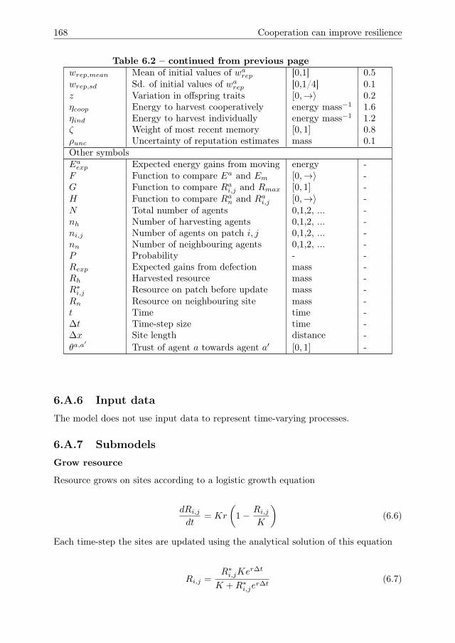
168 Cooperation can improve resilience
Table 6.2 – continued from previous pagewrep,mean Mean of initial values of warep [0,1] 0.5wrep,sd Sd. of initial values of warep [0,1/4] 0.1z Variation in offspring traits [0,→〉 0.2ηcoop Energy to harvest cooperatively energy mass−1 1.6ηind Energy to harvest individually energy mass−1 1.2ζ Weight of most recent memory [0, 1] 0.8ρunc Uncertainty of reputation estimates mass 0.1Other symbolsEaexp Expected energy gains from moving energy -F Function to compare Ea and Em [0,→〉 -G Function to compare Rai,j and Rmax [0, 1] -H Function to compare Ran and Rai,j [0,→〉 -N Total number of agents 0,1,2, ... -nh Number of harvesting agents 0,1,2, ... -ni,j Number of agents on patch i, j 0,1,2, ... -nn Number of neighbouring agents 0,1,2, ... -P Probability - -Rexp Expected gains from defection mass -Rh Harvested resource mass -R∗i,j Resource on patch before update mass -Rn Resource on neighbouring site mass -t Time time -∆t Time-step size time -∆x Site length distance -θa,a
′Trust of agent a towards agent a′ [0, 1] -
6.A.6 Input dataThe model does not use input data to represent time-varying processes.
6.A.7 SubmodelsGrow resource
Resource grows on sites according to a logistic growth equation
dRi,jdt
= Kr
(1− Ri,j
K
)(6.6)
Each time-step the sites are updated using the analytical solution of this equation
Ri,j =R∗i,jKe
r∆t
K +R∗i,jer∆t
(6.7)
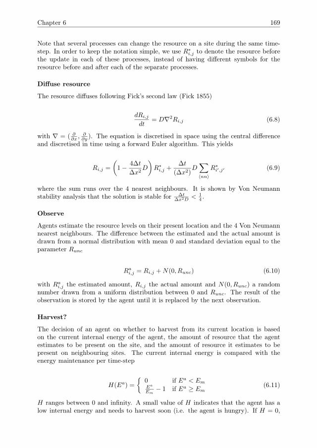
Chapter 6 169
Note that several processes can change the resource on a site during the same time-step. In order to keep the notation simple, we use R∗i,j to denote the resource beforethe update in each of these processes, instead of having different symbols for theresource before and after each of the separate processes.
Diffuse resource
The resource diffuses following Fick’s second law (Fick 1855)
dRi,jdt
= D∇2Ri,j (6.8)
with ∇ = ( ∂∂x ,
∂∂y ). The equation is discretised in space using the central difference
and discretised in time using a forward Euler algorithm. This yields
Ri,j =
(1− 4∆t
∆x2D
)R∗i,j +
∆t
(∆x2)D∑〈nn〉
R∗i′,j′ (6.9)
where the sum runs over the 4 nearest neighbours. It is shown by Von Neumannstability analysis that the solution is stable for ∆t
∆x2D < 14 .
Observe
Agents estimate the resource levels on their present location and the 4 Von Neumannnearest neighbours. The difference between the estimated and the actual amount isdrawn from a normal distribution with mean 0 and standard deviation equal to theparameter Runc
Rai,j = Ri,j +N(0, Runc) (6.10)
with Rai,j the estimated amount, Ri,j the actual amount and N(0, Runc) a randomnumber drawn from a uniform distribution between 0 and Runc. The result of theobservation is stored by the agent until it is replaced by the next observation.
Harvest?
The decision of an agent on whether to harvest from its current location is basedon the current internal energy of the agent, the amount of resource that the agentestimates to be present on the site, and the amount of resource it estimates to bepresent on neighbouring sites. The current internal energy is compared with theenergy maintenance per time-step
H(Ea) =
{0 if Ea < EmEa
Em− 1 if Ea ≥ Em
(6.11)
H ranges between 0 and infinity. A small value of H indicates that the agent has alow internal energy and needs to harvest soon (i.e. the agent is hungry). If H = 0,
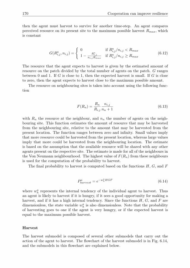
170 Cooperation can improve resilience
then the agent must harvest to survive for another time-step. An agent comparesperceived resource on its present site to the maximum possible harvest Rmax, whichis constant
G(Rai,j , ni,j) =
{0 if Rai,j/ni,j < Rmax
1− Rai,j
ni,jRmaxif Rai,j/ni,j ≥ Rmax
(6.12)
The resource that the agent expects to harvest is given by the estimated amount ofresource on the patch divided by the total number of agents on the patch. G rangesbetween 0 and 1. If G is close to 1, then the expected harvest is small. If G is closeto zero, then the agent expects to harvest close to the maximum possible amount.
The resource on neighbouring sites is taken into account using the following func-tion
F (Rn) =RnRi,j
ni,jnn + 1
(6.13)
with Rn the resource at the neighbour, and nn the number of agents on the neigh-bouring site. This function estimates the amount of resource that may be harvestedfrom the neighbouring site, relative to the amount that may be harvested from thepresent location. The function ranges between zero and infinity. Small values implythat more resource could be harvested from the present location, whereas large valuesimply that more could be harvested from the neighbouring location. The estimateis based on the assumption that the available resource will be shared with any otheragents present on the respective site. The estimate is made for all of the neighbours inthe Von Neumann neighbourhood. The highest value of F (Rn) from these neighboursis used for the computation of the probability to harvest.
The final probability to harvest is computed based on the functions H, G, and F
P aharvest = e−wahHGF (6.14)
where wah represents the internal tendency of the individual agent to harvest. Thusan agent is likely to harvest if it is hungry, if it sees a good opportunity for making aharvest, and if it has a high internal tendency. Since the functions H, G, and F aredimensionless, the state variable wah is also dimensionless. Note that the probabilityof harvesting goes to one if the agent is very hungry, or if the expected harvest isequal to the maximum possible harvest.
Harvest
The harvest submodel is composed of several other submodels that carry out theaction of the agent to harvest. The flowchart of the harvest submodel is in Fig. 6.14,and the submodels in this flowchart are explained below.
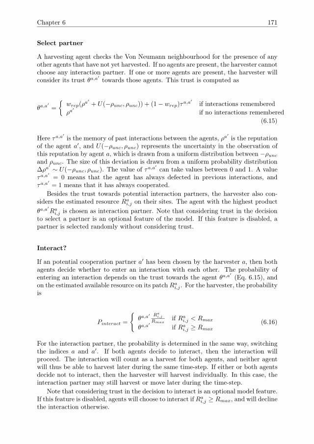
Chapter 6 171
Select partner
A harvesting agent checks the Von Neumann neighbourhood for the presence of anyother agents that have not yet harvested. If no agents are present, the harvester cannotchoose any interaction partner. If one or more agents are present, the harvester willconsider its trust θa,a
′towards those agents. This trust is computed as
θa,a′
=
{wrep(ρ
a′ + U(−ρunc, ρunc)) + (1− wrep)τa,a′
if interactions rememberedρa′
if no interactions remembered(6.15)
Here τa,a′is the memory of past interactions between the agents, ρa
′is the reputation
of the agent a′, and U(−ρunc, ρunc) represents the uncertainty in the observation ofthis reputation by agent a, which is drawn from a uniform distribution between −ρuncand ρunc. The size of this deviation is drawn from a uniform probability distribution∆ρa
′ ∼ U(−ρunc, ρunc). The value of τa,a′can take values between 0 and 1. A value
τa,a′
= 0 means that the agent has always defected in previous interactions, andτa,a
′= 1 means that it has always cooperated.
Besides the trust towards potential interaction partners, the harvester also con-siders the estimated resource Rai,j on their sites. The agent with the highest productθa,a
′Rai,j is chosen as interaction partner. Note that considering trust in the decision
to select a partner is an optional feature of the model. If this feature is disabled, apartner is selected randomly without considering trust.
Interact?
If an potential cooperation partner a′ has been chosen by the harvester a, then bothagents decide whether to enter an interaction with each other. The probability ofentering an interaction depends on the trust towards the agent θa,a
′(Eq. 6.15), and
on the estimated available resource on its patchRai,j . For the harvester, the probabilityis
Pinteract =
{θa,a
′ Rai,j
Rmaxif Rai,j < Rmax
θa,a′
if Rai,j ≥ Rmax(6.16)
For the interaction partner, the probability is determined in the same way, switchingthe indices a and a′. If both agents decide to interact, then the interaction willproceed. The interaction will count as a harvest for both agents, and neither agentwill thus be able to harvest later during the same time-step. If either or both agentsdecide not to interact, then the harvester will harvest individually. In this case, theinteraction partner may still harvest or move later during the time-step.
Note that considering trust in the decision to interact is an optional model feature.If this feature is disabled, agents will choose to interact if Rai,j ≥ Rmax, and will declinethe interaction otherwise.
172 Cooperation can improve resilience
Defect?
If both the interaction partner a and the harvester a′ have decided to interact, thenthe interaction partner will decide whether to cooperate or defect. The probability ofdefection is a weighted average of the trust the interaction partner has towards theharvester, as well as the internal tendency of the interaction partner to defect wdefect
Pdefect = wareciprocityθa,a′ + (1− wareciprocity)wadefect (6.17)
The value of the agent parameter wreciprocity thus determines the relative weight oftrust in the decision to defect.
Considering trust in the decision to defect is an optional feature of the model.If this feature is disabled, then the probability to defect will be given solely by theinternal tendency of the interaction partner Pdefect = wadefect.
Collect resource
The harvest is carried out by updating the amount of resource on the harvested sitei, j and the internal energy level of the harvesting agent. If there is an interactionpartner that decided to cooperate, the resource on its site is also updated. Eachagent can harvest up to a maximum of Rmax. If the amount of resource of the site isinsufficient to let an agent gather this maximum amount, then the available resourceis harvested. The updated amount of resource is Ri,j = R∗i,j − nhRh, with R∗i,j theamount before harvesting, nh the number of agents that are harvesting on a site, andRh the harvested amount per agent
Rh =
{R∗i,j if R∗i,j < nhRmaxRmax if R∗i,j > nhRmax
(6.18)
Harvesting costs energy per unit of resource collected. If agents are cooperatingon a harvest, then this additional cost is lowered when making the harvest. Thusηind > ηcoop, with ηind the energy cost per unit of resource for individual agents, andηcoop the cost for cooperating agents. If there is only a single harvesting agent, andno interaction partner, all of the collected resource is converted with efficiency c andadded to the internal energy
Ea = E∗a + cRh − ηindcRh. (6.19)
If there is an agent cooperating with the harvest, then both agents harvest fromtheir own location following Eq. 6.18, and share the total harvest equally
Ea = E∗a + c
(Rah +Ra
′
h
2
)− ηcoopcRah (6.20)
Ea′
= E∗a′+ c
(Rah +Ra
′
h
2
)− ηcoopcRa
′
h (6.21)
Chapter 6 173
with Rah the amount collected by the harvester and Ra′
h by the cooperating partner.Interaction partners that defect do not harvest anything, and spend only the initial
harvest cost Eh. The total harvest is still equally shared, so that
Ea = E∗a +cRah
2− ηindcRah (6.22)
Ea′
= E∗a′+cRah
2(6.23)
Note that the harvester a pays the energy cost ηind per unit of harvest, and thus doesnot receive any benefits from the interaction.
Update reputation and memory
After each harvest in which the harvester interacted with an interaction partner,the reputation of the interaction partner is lowered if it defected, and increased if itcooperated
ρa =
{(ρ∗,a − 1)ζ + 1 if the agent cooperatedρ∗,aζ if the agent defected (6.24)
This update ensures that all the previous decisions of an agent on whether or not to in-terfere are implicitly represented in its reputation score. The parameter ζ determineshow quick the reputation changes as a result of recent decisions. The most recentaction has a weight of 1− ζ. The old value, which contains all previous interactions,has a weight of ζ. If an agent does not interfere with harvests, then its reputationscore will move towards the maximum value of 1. If the agent does interfere, the scorewill move towards the minimum of zero.
The memories of the harvester about the interaction partner are updated in thesame way as the reputation
τa,a′
=
{(τ∗,a,a
′ − 1)ζ + 1 if the agent cooperatedτ∗,a,a
′ζ if the agent defected
(6.25)
Here τa,a′is the memory score of the harvester a regarding the interaction partner
a′, and τ∗,a,a′is the memory score before the update.
Move?
When deciding whether or not to move, an agent predicts how much resource itexpects to obtain at its current site and at the four nearest neighbouring sites. Forthis decision, the estimated resource present on the neighbouring sites is updated totake into account any changes in the resource amounts due to harvests. For its currentsite i, j the agent expects that the resource will be shared evenly among the agentson that site
Eaexp,i,j =cRai,jni,j
. (6.26)

174 Cooperation can improve resilience
For a neighbouring site, the agent expects that it will share the resource with theagents already present at the site. The agent also considers that it will first have tospend energy to move to a neighbouring site before harvesting there. Thus, the netexpected energy gain for the neighbouring site is equal to the expected harvest minusthe cost of moving to the site
Eaexp,k,l =cRak,lnk,l
− Emove. (6.27)
The expected energy gain of the current site is then compared with that of the nearestneighbour with the highest expected gain. Based on this comparison, the probabilityof moving is computed
Pmove = e−wamEexp,i,j/Eexp,k,l . (6.28)
Thus, an agent is likely to move if the expected energy gain is higher on a neigh-bouring site than on the present location. Since both the expected harvests have thedimensions of energy, the variable wam is dimensionless. This variable represents thedifferences between agents in their likeliness to move.
Move
The agent moves to the nearest neighbour with the highest value of Rai,j
ni,j. The location
of the agent is updated to the new site.
Maintenance
For each agent, the daily energy cost of maintenance is deducted from the internalenergy
Ea =
{0 if E∗a < EmE∗a − Em if E∗a ≥ Em
(6.29)
If the internal energy of the agent is lower than the maintenance costs, it will becomezero after paying maintenance. Because the ‘pay maintenance’ submodel is imme-diately followed by the ‘die?’ submodel, the agent will then die without taking anyfurther actions.
Die?
Every time-step, agents have a probability of dying or breeding, based on their internalenergy. The probability of dying is
Pdie(Ea) = e−vdE
a
(6.30)
Thus, the probability of dying goes to one as Ea goes to zero.

Chapter 6 175
Die
If an agent dies it is removed from the simulation.
Breed?
If an agent does not die, it has a probability of breeding
Pbreed(Ea) =
{0 if Ea < Eb1− e−vb(Ea−Eb) if Ea ≥ Eb
(6.31)
The submodel determines whether the agent will breed based on this probability.
Breed
If an agent breeds, it is replaced by two new agents. The energy of the parent issplit evenly among the two offspring. The values of wah and wam are inherited bythe offspring with some random deviation. The deviation is drawn from a uniformdistribution between ˘z and z. In some cases, the resulting value of wah and wam canbe negative. It is then set to zero instead. In the same way, the values of the weightswatrust and warep are also inherited.
6.A.8 Memory updateAgents remember previous interactions only for a limited number of time-steps. Thetime since the interaction between agents a and a′ is tracked as a state variable ha,a
′.
In the submodel, this age is increased by one. After this increase, if the time sincethe latest interaction exceeds the maximum memory length ha,a
′, then the memory
score is erased.
6.B One-factor-at-a-time results for growth rate r
In section 6.4.2 we have demonstrated the effects of increasing resource availabilityby increasing the carrying capacity K. For comparison, we offer here the effects ofincreasing the growth rate r. Similar to K, increasing values of r should cause anincrease in the availability of resource. Thus, we would expect similar results to thoseshown in section 6.4.2. Fig. B1 shows that for increasing r the population size nincreases approximately linearly in the model with mechanisms for cooperation. Inthe base model, in contrast, the population size increases for small values of r, butfor values of r ≥ 0.3, n starts to decrease. For values around r = 0.8 and larger, thepopulation collapses and almost goes to zero. Thus, the one-factor-at-a-time analysisfor r shows similar results to the one for K.
6.C Global sensitivity analysisTo explore the model behaviour under a wide range of parameter settings, we performa global sensitivity analysis, varying all model parameters simultaneously across the
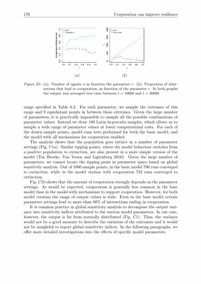
176 Cooperation can improve resilience
(a) (b)
Figure B1: (a): Number of agents n as function the parameter r. (b): Proportion of inter-actions that lead to cooperation, as function of the parameter r. In both graphsthe output was averaged over time between t = 10000 and t = 20000.
range specified in Table 6.2. For each parameter, we sample the extremes of thisrange and 9 equidistant points in between these extremes. Given the large numberof parameters, it is practically impossible to sample all the possible combinations ofparameter values. Instead we draw 100 Latin hypercube samples, which allows us tosample a wide range of parameter values at lower computational costs. For each ofthe drawn sample points, model runs were performed for both the basic model, andthe model with all mechanisms for cooperation enabled.
The analysis shows that the population goes extinct in a number of parametersettings (Fig. C1a). Similar tipping points, where the model behaviour switches froma positive population to extinction, are also present in a more simple version of themodel (Ten Broeke, Van Voorn and Ligtenberg 2016). Given the large number ofparameters, we cannot locate the tipping point in parameter space based on globalsensitivity analysis. Out of 1000 sample points, in the basic model 790 runs convergedto extinction, while in the model version with cooperation 722 runs converged toextinction.
Fig. C1b shows that the amount of cooperation strongly depends on the parametersettings. As would be expected, cooperation is generally less common in the basemodel than in the model with mechanisms to support cooperation. However, for bothmodel versions the range of output values is wide. Even in the base model certainparameter settings lead to more than 80% of interactions ending in cooperation.
It is common practice in global sensitivity analysis to decompose the output vari-ance into sensitivity indices attributed to the various model parameters. In our case,however, the output is far from normally distributed (Fig. C1). Thus, the variancewould not be a good measure to describe the variation of the outcomes and it wouldnot be insightful to report global sensitivity indices. In the following paragraphs, weoffer more detailed investigations into the effects of specific model parameters.
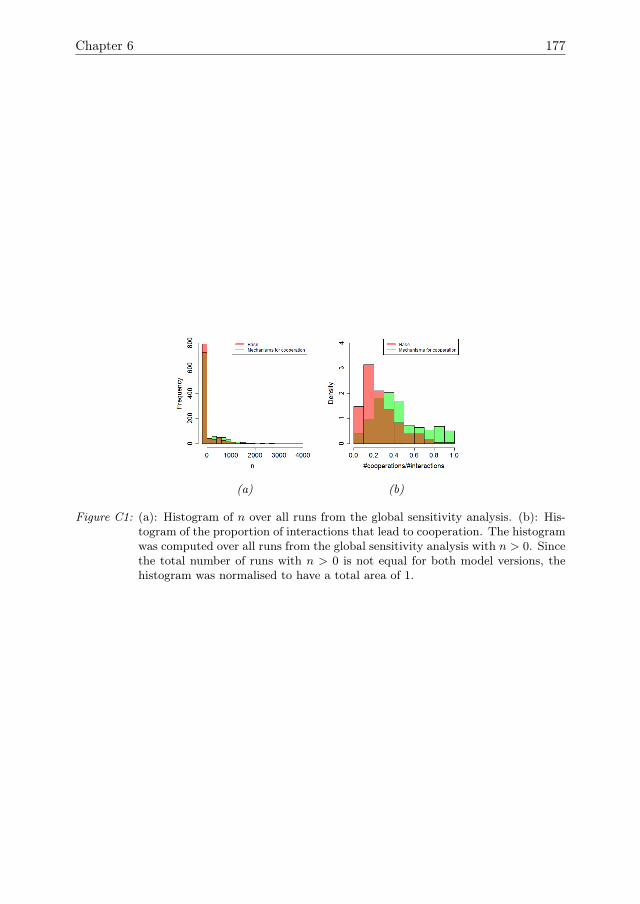
Chapter 6 177
(a) (b)
Figure C1: (a): Histogram of n over all runs from the global sensitivity analysis. (b): His-togram of the proportion of interactions that lead to cooperation. The histogramwas computed over all runs from the global sensitivity analysis with n > 0. Sincethe total number of runs with n > 0 is not equal for both model versions, thehistogram was normalised to have a total area of 1.

Chapter 7
General Discussion
Agent-based models (ABMs) are popular for modelling complex adaptive systems(CAS). However, the credibility and utility of ABMs for studying CAS is hamperedby a lack of available methodologies for analysing these models. It is partly dueto this lack of methodologies that many studies employing ABMs do not include asystematic sensitivity analysis (Thiele et al. 2014). Thus, there is a need for sensitivityanalysis methodologies that are suitable for ABMs. The main aim of this thesis is tocontribute to the development of such methodologies. To this end we have evaluatedthe strengths and limitations of existing sensitivity analysis methods. Furthermore,we have developed new methods to deal with challenges for which existing methodswere found to be insufficient.
7.1 Aims of sensitivity analysis
Before evaluating sensitivity analysis methodologies, it is crucial to discuss the aimsthat those methodologies are intended to serve. Although sensitivity analysis canserve a wide range of aims, most standard sensitivity analysis methods are designedto evaluate which parameters cause the most uncertainty in the model output. Inthis approach it is recommended to limit the analysis to a small number of outputvariables (Saltelli et al. 2008). The model parameters are then ranked according totheir influence on the output variables. This approach is demonstrated in Chapters 2(local sensitivity analysis) and 3 (global sensitivity analysis), and is commonly appliedin fields like engineering or chemistry. In these fields there is usually a relativelyhigh level of understanding of the modelled system, and a relatively low degree ofuncertainty. Therefore, accurate predictions are possible. Sensitivity analysis maythen help to further improve this accuracy by suggesting parameters for improvedmeasurements.
In most ABM applications, however, improving the accuracy of model predic-tions is not the main aim of sensitivity analysis. ABMs are typically used to modelopen systems with many uncertain factors. Although prediction in these systemsis not generally impossible (Helbing 2012, Troitzsch 2009), detailed predictions likein engineering systems are usually out of reach. A survey of a wide range of ABMstudies has concluded that not a single one of these studies was aimed at making
180 General Discussion
direct predictions (Heath et al. 2009). The number of ABM studies with this aimmay have increased since this survey, but still appears to be relatively low. Instead,many ABMs are used to explore whether a certain conceptual model can reproduceobserved behaviour of the real system (Heath et al. 2009, Macal 2016). Such an aimplaces entirely different demands on sensitivity analysis methodologies. Rather thanto identify influential parameters, sensitivity analysis is used to answer questions suchas the following:
• What kind of emergent behaviour may the model generate?
• Which model mechanisms are essential for generating this behaviour?
• To what extent is the emergent behaviour robust to parameter changes?
• What kind of behaviour is possible under different parameter regimes?
These kind of questions ask for a more qualitative kind of model assessment, whichtraditional sensitivity analysis methods are not designed to provide. This may explainto a large extent the short-comings of these methods for analysing ABMs.
7.2 Evaluation of sensitivity analysis methodologies
In this thesis a few traditional methods of sensitivity analysis have been evaluatedbased on their application to test-cases. Given the complexity of ABMs, and theirwide range of applications, any single sensitivity analysis methodology should notbe expected to be suitable for all ABM studies. As shown in Table 7.1, differentsensitivity analysis methodologies have different strengths and weaknesses. Thus, thechoice of sensitivity analysis methodology should depend on the types of interactionsin the model, as well as the aims of the analysis. In the following paragraphs wediscuss the strengths and weaknesses of each of the methods discussed in this thesis.
7.2.1 Local sensitivity analysis
Local sensitivity analysis was originally developed for ODE models, and has impor-tant applications for these models. For ABMs, however, its utility is limited. Localsensitivity analysis is based on partial derivatives of the model output with respect tothe model parameters. For ABMs, however, there are no equations available that re-late the parameters to the model outputs. As a result, the direct differential method,which is used to compute local sensitivities for ODE models, cannot be applied toABMs. Furthermore, most ABMs contain stochastic effects. For stochastic models,the partial derivatives are not well-defined. So, local sensitivity analysis cannot beapplied to ABMs without modifications. Apart from these limitations, for sensitivityanalysis of ABMs it is necessary to explore a wide range of parameter changes, forexample to assess the effects of interactions between parameters, or to detect tippingpoints. Local sensitivity analysis, in contrast, considers only small parameter changesaround a single point in parameter space. Therefore, local sensitivity analysis is notsuitable for assessing interaction effects or detecting tipping points in ABMs.
Chapter 7 181
7.2.2 Model-free global sensitivity analysis
Model-free sensitivity analysis is a form of global sensitivity analysis that is aimedat ranking model parameters based on the proportion of output variance explainedby each (combination of) parameters. The method is called model-free because noregression model is used in estimating these explained variances, in contrast withregression-based sensitivity analysis (Section 7.2.3). The output variance is esti-mated using Monte Carlo sampling. The use of the method has been advocatedfor ABMs by various authors (e.g. Cariboni et al. (2007), Ligmann-Zielinska et al.(2014), Fonoberova et al. (2013)). However, our results in Chapters 3 and 4 have re-vealed a number of practical and conceptual issues that limit the utility of model-freesensitivity analysis for ABMs.
A practical limitation is the relatively high computational cost of the method. InChapter 3, the method was applied to estimate sensitivity indices for 3 parametersof an ODE model describing predator-prey interaction. With a sample size of theorder of 104 model runs, significant uncertainties in the sensitivity estimates remained.Most ABMs contain a much larger number of parameters. For the relatively simpleABM discussed in Chapter 4, which contains 15 parameters, the sensitivities couldnot be accurately estimated even with a sample size of 17.000 model runs. Due tothis inaccuracy, some sensitivity indices were estimated to be negative, which has norealistic interpretation. For these results, the sampling design suggested by Saltelli(2002) was used. Other sampling designs have been explored in Chapter 3. Some ofthese other designs might yield more accurate estimates, but the computational costsare expected to be extremely high.
A second issue is that whereas model-free global sensitivity analysis expresses thesensitivity indices in terms of explained variance, for many ABMs the variance isnot a good measure to describe the variation in the model output. If the modeloutput is normally distributed, then its variation is fully described by the variance.For many ABMs, such as the one discussed in Chapter 4, the output distributionis far from normal. The variance is then insufficient to describe the variation of theoutput. Thus, before applying model-free global sensitivity analysis, it should alwaysbe verified whether the model output is normally distributed.
A more conceptual issue is that the aggregation of model output across a region ofparameter space leads to a loss of detailed information that is crucial for understandingmodel behaviour. ABMs generate large amounts of output data, both on the agent-level and on the system-level. Considering only aggregated output on the system-level does not yield insight in the emergence of system-level properties from lower-level agent interactions. It may show that some parameter is influential, but notwhy it it influential. Therefore, considering only aggregated system-level outputsseems contradictory to the CAS approach, since CAS is a bottom-up approach inwhich system-level properties emerge from lower-level interactions. Given the issuesdescribed above, model-free global sensitivity analysis appears to be only of limiteduse for most ABM studies.
7.2.3 Regression-based sensitivity analysis
Similar to model-free global sensitivity analysis, regression-based sensitivity analysisexpresses parameter sensitivities in terms of explained output variance. The main

182 General Discussion
difference between both methods is that in regression-based sensitivity analysis aregression model is fitted to the ABM output. The explained output variance foreach parameter is then computed based on the regression model. Thanks to the useof a regression model, regression-based sensitivity analysis is computationally cheaperthan model-free sensitivity analysis. However, the method requires a regression modelthat yields a good fit to the model output. For ABMs finding such a regressionmodel is typically not a straightforward task, because the relationships between theparameters and the model outputs may be complex and may change over time. For thetest-case in Chapter 4, the difficulty of finding an acceptable fit proved to be a majorlimitation. The method also suffers from most of the limitations that were discussedabove for model-free sensitivity global sensitivity analysis. Thus, if the aim is to rankthe model parameters in terms of their explained variance, then regression-basedsensitivity analysis may serve as a computationally cheaper alternative for model-freeglobal sensitivity analysis, if a suitable regression model is found. Otherwise, the useof other methods is recommended.
7.2.4 One-factor-at-a-time sensitivity analysis
One-factor-at-a-time (OFAT) sensitivity analysis evaluates the output for a range ofvalues for one of the parameters, while keeping all other parameters constant. Themain advantage of OFAT is that it isolates the effect of individual parameters. Foreach parameter, OFAT shows how changes in that parameter affect the output, forexample whether the output is increased or decreased, whether this relationship islinear or non-linear, and whether parameter changes may cause a tipping point. InChapter 3, OFAT was applied to an ODE model for the purpose of tipping pointdetection. The results revealed the same tipping points that may be detected usingbifurcation analysis. For the ABM in Chapter 4, for which bifurcation analysis is notapplicable, OFAT also revealed a number of tipping points. The main limitation ofOFAT is that since it considers only variations in individual parameters, it cannotbe used to explore interaction effects. As a result, it may fail to detect tippingpoints that are only found if multiple parameters are simultaneously changed. Itis therefore recommended to supplement OFAT with a global method of sensitivityanalysis. Nevertheless, OFAT serves as a good starting point for analysing ABMsand detecting tipping points. Furthermore, the computational costs of OFAT arerelatively low.
7.2.5 All-but-one-at-a-time sensitivity analysis
All-but-one-at-a-time sensitivity analysis (ABOS) is a graphical method of globalsensitivity analysis that has been discussed in Chapter 3. Application of ABOS maybe based on the same samples that are used for model-free global sensitivity analysisor regression-based global sensitivity analysis. In ABOS the output of those samplesis plotted as a function of one parameter, while all other parameters are varied.ABOS can help to reveal the effects of individual parameters, but unlike OFAT italso explores interaction effects. A limitation of ABOS is that it is computationallyexpensive. This limitation becomes irrelevant if ABOS is performed in addition toregression-based global sensitivity analysis or model-free global sensitivity analysis, in
Chapter 7 183
which case it uses the same samples and thus does not impose addition computationalcosts. A disadvantage of ABOS is that in case of a large number of parameters itmay become difficult to graphically identify the effects of individual parameters.
7.2.6 Earth-mover’s distance
Sensitivity analysis using the earth-mover’s distance is discussed in Chapter 5. In thismethod, probability density functions (PDF)s of the model output are compared fordifferent model versions or settings. The earth-mover’s distance is used to quantify thedifference between PDFs. Using the full PDF, rather than summarising measures likethe mean or variance ensures that no information is lost due to aggregating output.The PDF may be composed either of repeated model runs each measured at thesame time, or of a single model run repeatedly measured over time. By comparingthese two for adaptive and non-adaptive model versions, the method may be usedto measure the effects of adaptation. Although in this thesis the method was usedexclusively for the purpose of measuring adaptation, it could also be used as a moregeneral sensitivity measure for the effects of other factors on the model output.
7.3 Lessons from applying sensitivity analysis toABMs
An important use of the ABM test-cases in this thesis has been to explore the effectsof loosening simplifying assumptions imposed by other modelling methods. For exam-ple, ODE predator-prey models assume that individuals are identical and influenceeach other equally. Or, game models assume that agents follow economic rationality.In some cases, such simplifying assumptions may help to reveal core mechanics of thesystem. In other cases, however, they are over-simplifications. ABMs generally re-quire a lower level of simplification than other modelling methods. Therefore ABMscan be used to verify whether relevant characteristics of the system are neglectedthrough the simplifications of other methods. For example, in economic systems fac-tors such as emotional attachment to a business can be strongly influential (Libreet al. 2015). ABMs are suitable for modelling such factors, that are neglected intraditional economic models. Thus, ABMs can contribute to a greater understandingof the system by showing that factors that are neglected by traditional modellingmethods can have a significant impact on the system.
The downside of using ABMs compared to most other modelling methods is aloss of analytic tractability. The sensitivity analysis methodologies proposed in thisthesis are intended to help mitigate this downside, and increase the utility of ABMs.The ABMs discussed in this thesis serve as examples of how sensitivity analysis maybe used to obtain more information from ABMs. The main topics that have beeninvestigated using these ABMs are adaptation and resilience, and the evolution ofcooperation.
184 General Discussion
7.3.1 Adaptation and resilience
Resilience is currently a widely discussed topic in the context of SES. However, def-initions of resilience vary strongly across the scientific literature (Grimm and Wissel1997). Often resilience is explained in terms of a metaphorical potential landscape.Potential landscapes have been commonly used in physics, for example in classicalmechanics, electrodynamics, or quantum physics. In these applications, the potentialenergy has a clear meaning in terms of the motion of bodies under influence from aforce. For example, bodies under influence from the gravitational force are naturallyattracted to each other, and tend to minimise their potential energy by moving to-wards each other. While the concept of potential is frequently used as a metaphor todescribe the resilience of SES, it is unclear to what extent this way of thinking trans-lates to real-life SES. For example, it is usually unclear what aspect(s) of the real-lifesystem the potential energy would correspond to. As a result, definitions of resilienceare often vague and vary strongly between applications. Furthermore, when appliedto SES, thinking in terms of potential landscapes might lead to misleading insights.For example, it is implied that there exist (local) minima in terms of potential energythat the system is naturally attracted towards. For most real-life SES, however, it isnot known whether there exist stable states that the system is attracted towards, orwhether the system would continuously keep moving towards new states.
Thus, to apply the concept of resilience in real-life cases, there is a need to bevery specific about precisely what is meant by resilience. For example, it is crucial tospecify what aspects of the system should be resilient, and what kind of pressures orshocks it should be resilient to (Carpenter et al. 2001). Furthermore, it needs to bespecified how the resilience of these aspects is operationalised, for example in termsof return time, or stability of some system state. Simulation models can be helpful inensuring that the concept of resilience in SES, as well as the mechanisms underlyingthis resilience are properly formalised. Furthermore, it helps the user to test the logi-cal consistence of these mechanisms. For example, adaptation is commonly suggestedto be an important source of resilience in SES (Walker et al. 2004), but few studieshave verified this. In Chapter 5 an ABM was used to examine the effects of agentadaptation on the resilience of a population of agents competing for a renewable re-source. Using OFAT sensitivity analysis it was shown that the model contains tippingpoints that lead to extinction of the population when crossed. To examine how adap-tation affects the resilience of the population against this extinction, a model versionwith adaptation was compared to a version that includes adaptation through naturalselection. It it shown that adaptation leads to a larger population size, and makesthe population more resilient to extinction. While extinction still occurs for certainparameter settings, the parameter range for which the population remains positive isincreased. Although the model discussed in this thesis may be relatively abstract, itshows how simulation modelling can be used to give a measurable interpretation tothe concept of resilience that may be used for real-life applications.
7.3.2 Cooperation
The evolution of cooperation has been studied extensively using game theory models.Such models show that indirect reciprocity may be an important mechanism to sup-port cooperation Nowak and Sigmund (2005). However, game theory models impose
Chapter 7 185
strict assumptions. For example, benefits from cooperation are pre-defined and con-stant throughout the simulation. Furthermore, ecological dynamics such as changesin population size due to cooperation are usually not taken into account (Doebeli andHauert 2005, Gotts et al. 2003). For common-pool resource systems, however, suchdynamics may be crucial. For example, a high level of cooperation might lead to anincreasing population size, which in turn can decrease resource availability.
ABMs provide a useful tool for including ecological dynamics, and loosening someof the assumptions of game theory models. To this end, the ABM of Chapter 5was extended to include cooperation between agents. Using OFAT, it was shownthat ecological dynamics strongly influence cooperation. For instance, in absence ofindirect reciprocity, both the level of cooperation and the population size decrease.The decreased population size, however, leads to the formation of small groups. Thesesmall groups show an increased level of cooperation. Thus, due to population sizeeffects and group formation, cooperation is maintained even in absence of any explicitmechanisms to support it. This shows that it is important to consider ecologicalfactors in studies on evolution of cooperation. That these factors are omitted in moststudies may be largely because they quickly lead to highly complex models. ABMs,when combined with suitable analysis methodologies, may be of great value to studythe effect of ecological factors on the evolution of cooperation.
7.4 Future workThe utility of sensitivity analysis methodologies for ABMs would be further improvedby the development of software to automate their application to ABMs. Currentlymost software for ABMs features only limited possibilities for performing a systematicsensitivity analysis. For example, whereas Netlogo (Wilensky 1999) contains somesupport for sensitivity analysis, it does not contain support for most designs of globalsensitivity analysis. As a result, performing such an analysis is time-consuming. Animportant requirement for software to automate sensitivity analysis for ABMs isthat a wide range of options for storing and visualising output are offered. Whereastraditional sensitivity analysis usually focuses on a small number of outputs, ABMscan generate large amounts of data each time-step, both on the system-level and onthe level of individual agents. Therefore, ensuring that the different types of outputdata are easily stored, accessed, and visualised is even more important for ABMsthan for other modelling methods. Steps towards more practical and user-friendlyapplication of sensitivity analysis have already been made in the form of tools likeMEME (Ivanyi et al. 2007) and RNetlogo (Thiele et al. 2014).
Traditional sensitivity analysis methodologies focus on examining a small numberof outputs, and creating high-level summaries of the effects of each model parame-ter on these outputs. Agent-based models generate large amounts of output becauseeach individual agent possesses its own values for state variables. Thus, focussingonly on a few global outputs means that a lot of information is discarded before theanalysis takes place (Macal 2016, Nelson 2016). Progress may be made by collectingmore information on agent-level variables as part of model analysis. For example, inChapter 6 distributions of agent-level variables were used to better understand resultsfrom OFAT sensitivity analysis. However, relationships between agent variables, orbetween agent variables and system-level output, were not yet examined. The de-

186 General Discussion
velopment of methodologies to detect such relationships may help to better analyseABMs. Standard sensitivity analysis methods that are currently available for ABMsessentially consider all the intermediate processes as a ’black box’. Including examina-tion of these processes as part of sensitivity analysis will require a different approachtowards sensitivity analysis. Tools for finding relationships in large amounts of datahave become available in other fields (Nelson 2016). Although the analysis of ABMsposes its own challenges, application of methods from these fields may be a good steptowards a better use of sensitivity analysis to examine causal relationships containedin ABM output.

Chapter 7 187
Tab
le7.
1:Aim
san
dlimitationsof
sensitivity
analysis
(SA)method
s.
Metho
dology
Streng
thLimitations
LocalS
ARan
king
parameter
sensitivitiesarou
nddefault
parameter
setting
Doesno
treveal
interactioneff
ects.Im
plem
enta-
tion
prob
lemsforA
BMs
Regression-ba
sed
glob
alSA
Ran
king
parameter
sensitivitiesacross
aregion
ofpa
rameter
space
Com
putation
ally
expe
nsive.
Inform
ation
lost
during
aggregation.
Diffi
cult
tofin
dago
odfit
forA
BMs.
Mod
el-free
glob
alSA
Ran
king
parameter
sensitivitiesacross
aregion
ofpa
rameter
space
Com
putation
ally
expe
nsive.
Inform
ation
lost
during
aggregation.
Doesno
tconsider
tipp
ing
points.
OFAT
Und
erstan
ding
effects
ofspecificpa
rameterson
mod
elbe
haviou
r,tipp
ingpo
intdetection
Doesno
tconsider
interactioneff
ects
AB
OS
Und
erstan
ding
effects
ofgrou
psof
parameterson
mod
elbe
haviou
rCom
putation
ally
expe
nsive.
Graph
smay
become
clutteredforlargenu
mbe
rof
parameters
Earth-m
over’s
distan
ceAssessing
time-depe
ndence
andeff
ects
ofad
apta-
tion
Doesno
tconsider
parameter
interactions.
Re-
quires
sepa
rate
adap
tation
mecha
nism
.

References
Allee, W. C.: 1931, Animal aggregations: A study in general sociology., University ofChicago, Chicago .
Alliance, R.: 2010, Assessing resilience in social-ecological systems: Workbook forpractitioners.
Archer, G. E. B., Saltelli, A. and Sobol, I. M.: 1997, Sensitivity measures, anova-like techniques and the use of bootstrap, Journal of Statistical Computation andSimulation 58(2), 99–120.
Aubert-Kato, N., Witkowski, O. and Ikegami, T.: 2015, The hunger games: Embodiedagents evolving foraging strategies on the frugal-greedy spectrum, Proceedings ofthe European Conference on Artificial Life pp. 357–364.
Auder, B. and Iooss, B.: 2008, Global sensitivity analysis based on entropy, Safety,reliability and risk analysis-Proceedings of the ESREL 2008 Conference, pp. 2107–2115.
Augusiak, J., Van den Brink, P. J. and Grimm, V.: 2014, Merging validation andevaluation of ecological models to ‘evaludation’: a review of terminology and apractical approach, Ecological Modelling 280, 117–128.
Axtell, R.: 1999, Why agents?: on the varied motivations for agent computing inthe social sciences, Why agents? on the varied motivations for agent computingin the social sciences. In Macal, C. M. & Sallach, D. (Eds.), Proceedings of theWorkshop on Agent Simulation: Applications, Models, and Tools, Center on Socialand Economic Dynamics Washington, DC.
Banks, H. T., Dediu, S. and Ernstberger, S. L.: 2007, Sensitivity functions and theiruses in inverse problems, Journal of Inverse and Ill posed problems 15(7), 683.
Basurto, X., Gelcich, S. and Ostrom, E.: 2013, The social–ecological system frame-work as a knowledge classificatory system for benthic small-scale fisheries, GlobalEnvironmental Change 23(6), 1366–1380.
Bazykin, A. D.: 1998, Nonlinear dynamics of interacting populations, Vol. 11, WorldScientific.
Bear, A. and Rand, D. G.: 2016, Intuition, deliberation, and the evolution of cooper-ation, Proceedings of the National Academy of Sciences 113(4), 936–941.
Bendat, J. S. and Piersol, A. G.: 2011, Random data: analysis and measurementprocedures, Vol. 729, John Wiley & Sons.
Boettiger, C., Ross, N. and Hastings, A.: 2013, Early warning signals: the chartedand uncharted territories, Theoretical ecology 6(3), 255–264.
Borgonovo, E.: 2007, A new uncertainty importance measure, Reliability Engineering& System Safety 92(6), 771–784.
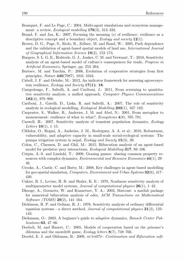
190 References
Bousquet, F. and Le Page, C.: 2004, Multi-agent simulations and ecosystem manage-ment: a review, Ecological modelling 176(3), 313–332.
Brand, F. and Jax, K.: 2007, Focusing the meaning (s) of resilience: resilience as adescriptive concept and a boundary object, Ecology and society 12(1).
Brown, D. G., Page, S., Riolo, R., Zellner, M. and Rand, W.: 2005, Path dependenceand the validation of agent-based spatial models of land use, International Journalof Geographical Information Science 19(2), 153–174.
Burgers, S. L. G. E., Hofstede, G. J., Jonker, C. M. and Verwaart, T.: 2010, Sensitivityanalysis of an agent-based model of culture’s consequences for trade, Progress inArtificial Economics, Springer, pp. 253–264.
Burtsev, M. and Turchin, P.: 2006, Evolution of cooperative strategies from firstprinciples, Nature 440(7087), 1041–1044.
Cabell, J. F. and Oelofse, M.: 2012, An indicator framework for assessing agroecosys-tem resilience, Ecology and Society 17(1): 18.
Campolongo, F., Saltelli, A. and Cariboni, J.: 2011, From screening to quantita-tive sensitivity analysis. a unified approach, Computer Physics Communications182(4), 978–988.
Cariboni, J., Gatelli, D., Liska, R. and Saltelli, A.: 2007, The role of sensitivityanalysis in ecological modelling, Ecological Modelling 203(1), 167–182.
Carpenter, S., Walker, B., Anderies, J. M. and Abel, N.: 2001, From metaphor tomeasurement: resilience of what to what?, Ecosystems 4(8), 765–781.
Caswell, H.: 2007, Sensitivity analysis of transient population dynamics, EcologyLetters 10(1), 1–15.
Cifdaloz, O., Regmi, A., Anderies, J. M., Rodriguez, A. A. et al.: 2010, Robustness,vulnerability, and adaptive capacity in small-scale social-ecological systems: Thepumpa irrigation system in nepal, Ecology and Society 15(3), 39.
Colon, C., Claessen, D. and Ghil, M.: 2015, Bifurcation analysis of an agent-basedmodel for predator–prey interactions, Ecological Modelling 317, 93–106.
Crépin, A.-S. and Lindahl, T.: 2009, Grazing games: sharing common property re-sources with complex dynamics, Environmental and Resource Economics 44(1), 29–46.
Crooks, A., Castle, C. and Batty, M.: 2008, Key challenges in agent-based modellingfor geo-spatial simulation, Computers, Environment and Urban Systems 32(6), 417–430.
Cukier, R. I., Levine, H. B. and Shuler, K. E.: 1978, Nonlinear sensitivity analysis ofmultiparameter model systems, Journal of computational physics 26(1), 1–42.
Dhooge, A., Govaerts, W. and Kuznetsov, Y. A.: 2003, Matcont: a matlab packagefor numerical bifurcation analysis of odes, ACM Transactions on MathematicalSoftware (TOMS) 29(2), 141–164.
Dickinson, R. P. and Gelinas, R. J.: 1976, Sensitivity analysis of ordinary differentialequation systems - a direct method, Journal of computational physics 21(2), 123–143.
Diekmann, O.: 2003, A beginner’s guide to adaptive dynamics, Banach Center Pub-lications 63, 47–86.
Doebeli, M. and Hauert, C.: 2005, Models of cooperation based on the prisoner’sdilemma and the snowdrift game, Ecology letters 8(7), 748–766.
Doedel, E. J. and Oldeman, B.: 2009, auto07p: Continuation and Bifurcation soft-
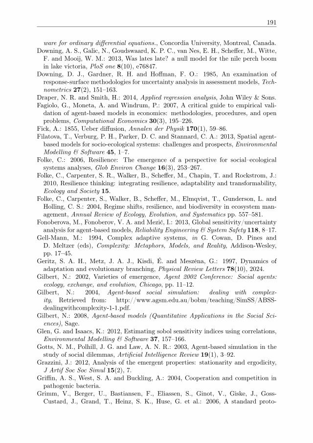
191
ware for ordinary differential equations., Concordia University, Montreal, Canada.Downing, A. S., Galic, N., Goudswaard, K. P. C., van Nes, E. H., Scheffer, M., Witte,
F. and Mooij, W. M.: 2013, Was lates late? a null model for the nile perch boomin lake victoria, PloS one 8(10), e76847.
Downing, D. J., Gardner, R. H. and Hoffman, F. O.: 1985, An examination ofresponse-surface methodologies for uncertainty analysis in assessment models, Tech-nometrics 27(2), 151–163.
Draper, N. R. and Smith, H.: 2014, Applied regression analysis, John Wiley & Sons.Fagiolo, G., Moneta, A. and Windrum, P.: 2007, A critical guide to empirical vali-
dation of agent-based models in economics: methodologies, procedures, and openproblems, Computational Economics 30(3), 195–226.
Fick, A.: 1855, Ueber diffusion, Annalen der Physik 170(1), 59–86.Filatova, T., Verburg, P. H., Parker, D. C. and Stannard, C. A.: 2013, Spatial agent-
based models for socio-ecological systems: challenges and prospects, EnvironmentalModelling & Software 45, 1–7.
Folke, C.: 2006, Resilience: The emergence of a perspective for social–ecologicalsystems analyses, Glob Environ Change 16(3), 253–267.
Folke, C., Carpenter, S. R., Walker, B., Scheffer, M., Chapin, T. and Rockstrom, J.:2010, Resilience thinking: integrating resilience, adaptability and transformability,Ecology and Society 15.
Folke, C., Carpenter, S., Walker, B., Scheffer, M., Elmqvist, T., Gunderson, L. andHolling, C. S.: 2004, Regime shifts, resilience, and biodiversity in ecosystem man-agement, Annual Review of Ecology, Evolution, and Systematics pp. 557–581.
Fonoberova, M., Fonoberov, V. A. and Mezić, I.: 2013, Global sensitivity/uncertaintyanalysis for agent-based models, Reliability Engineering & System Safety 118, 8–17.
Gell-Mann, M.: 1994, Complex adaptive systems, in G. Cowan, D. Pines andD. Meltzer (eds), Complexity: Metaphors, Models, and Reality, Addison-Wesley,pp. 17–45.
Geritz, S. A. H., Metz, J. A. J., Kisdi, É. and Meszéna, G.: 1997, Dynamics ofadaptation and evolutionary branching, Physical Review Letters 78(10), 2024.
Gilbert, N.: 2002, Varieties of emergence, Agent 2002 Conference: Social agents:ecology, exchange, and evolution, Chicago, pp. 11–12.
Gilbert, N.: 2004, Agent-based social simulation: dealing with complex-ity, Retrieved from: http://www.agsm.edu.au/bobm/teaching/SimSS/ABSS-dealingwithcomplexity-1-1.pdf.
Gilbert, N.: 2008, Agent-based models (Quantitative Applications in the Social Sci-ences), Sage.
Glen, G. and Isaacs, K.: 2012, Estimating sobol sensitivity indices using correlations,Environmental Modelling & Software 37, 157–166.
Gotts, N. M., Polhill, J. G. and Law, A. N. R.: 2003, Agent-based simulation in thestudy of social dilemmas, Artificial Intelligence Review 19(1), 3–92.
Grazzini, J.: 2012, Analysis of the emergent properties: stationarity and ergodicity,J Artif Soc Soc Simul 15(2), 7.
Griffin, A. S., West, S. A. and Buckling, A.: 2004, Cooperation and competition inpathogenic bacteria.
Grimm, V., Berger, U., Bastiansen, F., Eliassen, S., Ginot, V., Giske, J., Goss-Custard, J., Grand, T., Heinz, S. K., Huse, G. et al.: 2006, A standard proto-
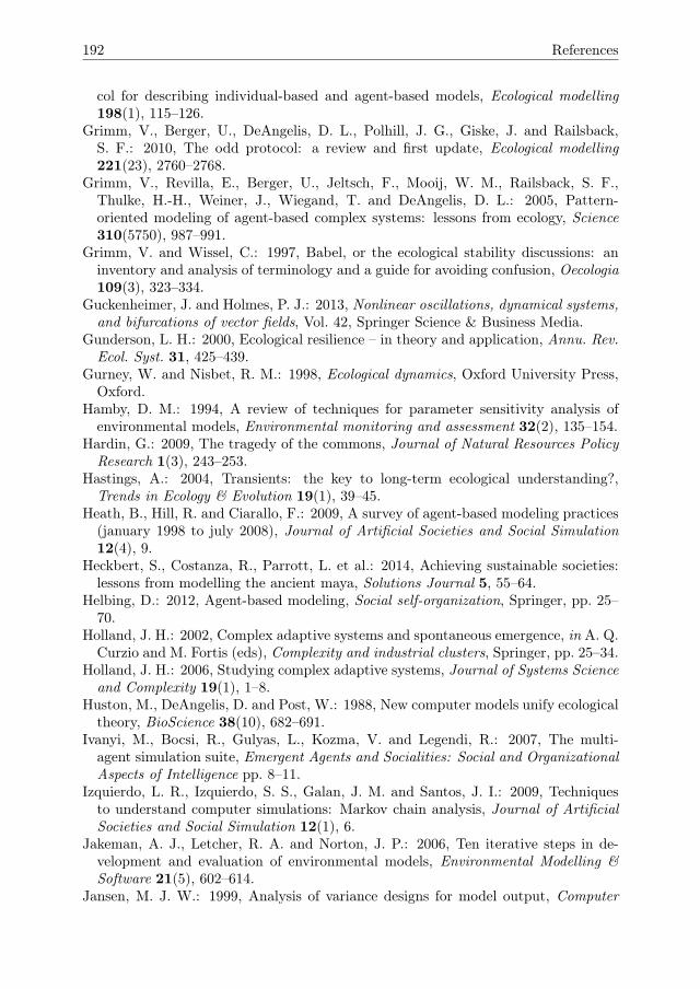
192 References
col for describing individual-based and agent-based models, Ecological modelling198(1), 115–126.
Grimm, V., Berger, U., DeAngelis, D. L., Polhill, J. G., Giske, J. and Railsback,S. F.: 2010, The odd protocol: a review and first update, Ecological modelling221(23), 2760–2768.
Grimm, V., Revilla, E., Berger, U., Jeltsch, F., Mooij, W. M., Railsback, S. F.,Thulke, H.-H., Weiner, J., Wiegand, T. and DeAngelis, D. L.: 2005, Pattern-oriented modeling of agent-based complex systems: lessons from ecology, Science310(5750), 987–991.
Grimm, V. and Wissel, C.: 1997, Babel, or the ecological stability discussions: aninventory and analysis of terminology and a guide for avoiding confusion, Oecologia109(3), 323–334.
Guckenheimer, J. and Holmes, P. J.: 2013, Nonlinear oscillations, dynamical systems,and bifurcations of vector fields, Vol. 42, Springer Science & Business Media.
Gunderson, L. H.: 2000, Ecological resilience – in theory and application, Annu. Rev.Ecol. Syst. 31, 425–439.
Gurney, W. and Nisbet, R. M.: 1998, Ecological dynamics, Oxford University Press,Oxford.
Hamby, D. M.: 1994, A review of techniques for parameter sensitivity analysis ofenvironmental models, Environmental monitoring and assessment 32(2), 135–154.
Hardin, G.: 2009, The tragedy of the commons, Journal of Natural Resources PolicyResearch 1(3), 243–253.
Hastings, A.: 2004, Transients: the key to long-term ecological understanding?,Trends in Ecology & Evolution 19(1), 39–45.
Heath, B., Hill, R. and Ciarallo, F.: 2009, A survey of agent-based modeling practices(january 1998 to july 2008), Journal of Artificial Societies and Social Simulation12(4), 9.
Heckbert, S., Costanza, R., Parrott, L. et al.: 2014, Achieving sustainable societies:lessons from modelling the ancient maya, Solutions Journal 5, 55–64.
Helbing, D.: 2012, Agent-based modeling, Social self-organization, Springer, pp. 25–70.
Holland, J. H.: 2002, Complex adaptive systems and spontaneous emergence, in A. Q.Curzio and M. Fortis (eds), Complexity and industrial clusters, Springer, pp. 25–34.
Holland, J. H.: 2006, Studying complex adaptive systems, Journal of Systems Scienceand Complexity 19(1), 1–8.
Huston, M., DeAngelis, D. and Post, W.: 1988, New computer models unify ecologicaltheory, BioScience 38(10), 682–691.
Ivanyi, M., Bocsi, R., Gulyas, L., Kozma, V. and Legendi, R.: 2007, The multi-agent simulation suite, Emergent Agents and Socialities: Social and OrganizationalAspects of Intelligence pp. 8–11.
Izquierdo, L. R., Izquierdo, S. S., Galan, J. M. and Santos, J. I.: 2009, Techniquesto understand computer simulations: Markov chain analysis, Journal of ArtificialSocieties and Social Simulation 12(1), 6.
Jakeman, A. J., Letcher, R. A. and Norton, J. P.: 2006, Ten iterative steps in de-velopment and evaluation of environmental models, Environmental Modelling &Software 21(5), 602–614.
Jansen, M. J. W.: 1999, Analysis of variance designs for model output, Computer
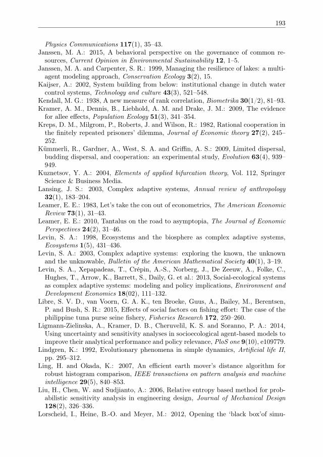
193
Physics Communications 117(1), 35–43.Janssen, M. A.: 2015, A behavioral perspective on the governance of common re-
sources, Current Opinion in Environmental Sustainability 12, 1–5.Janssen, M. A. and Carpenter, S. R.: 1999, Managing the resilience of lakes: a multi-
agent modeling approach, Conservation Ecology 3(2), 15.Kaijser, A.: 2002, System building from below: institutional change in dutch water
control systems, Technology and culture 43(3), 521–548.Kendall, M. G.: 1938, A new measure of rank correlation, Biometrika 30(1/2), 81–93.Kramer, A. M., Dennis, B., Liebhold, A. M. and Drake, J. M.: 2009, The evidence
for allee effects, Population Ecology 51(3), 341–354.Kreps, D. M., Milgrom, P., Roberts, J. and Wilson, R.: 1982, Rational cooperation in
the finitely repeated prisoners’ dilemma, Journal of Economic theory 27(2), 245–252.
Kümmerli, R., Gardner, A., West, S. A. and Griffin, A. S.: 2009, Limited dispersal,budding dispersal, and cooperation: an experimental study, Evolution 63(4), 939–949.
Kuznetsov, Y. A.: 2004, Elements of applied bifurcation theory, Vol. 112, SpringerScience & Business Media.
Lansing, J. S.: 2003, Complex adaptive systems, Annual review of anthropology32(1), 183–204.
Leamer, E. E.: 1983, Let’s take the con out of econometrics, The American EconomicReview 73(1), 31–43.
Leamer, E. E.: 2010, Tantalus on the road to asymptopia, The Journal of EconomicPerspectives 24(2), 31–46.
Levin, S. A.: 1998, Ecosystems and the biosphere as complex adaptive systems,Ecosystems 1(5), 431–436.
Levin, S. A.: 2003, Complex adaptive systems: exploring the known, the unknownand the unknowable, Bulletin of the American Mathematical Society 40(1), 3–19.
Levin, S. A., Xepapadeas, T., Crépin, A.-S., Norberg, J., De Zeeuw, A., Folke, C.,Hughes, T., Arrow, K., Barrett, S., Daily, G. et al.: 2013, Social-ecological systemsas complex adaptive systems: modeling and policy implications, Environment andDevelopment Economics 18(02), 111–132.
Libre, S. V. D., van Voorn, G. A. K., ten Broeke, Guus, A., Bailey, M., Berentsen,P. and Bush, S. R.: 2015, Effects of social factors on fishing effort: The case of thephilippine tuna purse seine fishery, Fisheries Research 172, 250–260.
Ligmann-Zielinska, A., Kramer, D. B., Cheruvelil, K. S. and Soranno, P. A.: 2014,Using uncertainty and sensitivity analyses in socioecological agent-based models toimprove their analytical performance and policy relevance, PloS one 9(10), e109779.
Lindgren, K.: 1992, Evolutionary phenomena in simple dynamics, Artificial life II,pp. 295–312.
Ling, H. and Okada, K.: 2007, An efficient earth mover’s distance algorithm forrobust histogram comparison, IEEE transactions on pattern analysis and machineintelligence 29(5), 840–853.
Liu, H., Chen, W. and Sudjianto, A.: 2006, Relative entropy based method for prob-abilistic sensitivity analysis in engineering design, Journal of Mechanical Design128(2), 326–336.
Lorscheid, I., Heine, B.-O. and Meyer, M.: 2012, Opening the ‘black box’of simu-
194 References
lations: increased transparency and effective communication through the system-atic design of experiments, Computational and Mathematical Organization Theory18(1), 22–62.
Louzoun, Y. and Solomon, S.: 2004, Proliferation and competition in discrete biolog-ical systems, New Directions in Statistical Physics, Springer, pp. 225–242.
Macal, C. M.: 2016, Everything you need to know about agent-based modelling andsimulation, Journal of Simulation 10(2), 144–156.
Macal, C. M. and North, M. J.: 2009, Agent-based modeling and simulation, Wintersimulation conference, Winter simulation conference, pp. 86–98.
Macal, C. M. and North, M. J.: 2010, Tutorial on agent-based modelling and simula-tion, Journal of simulation 4(3), 151–162.
Mann, H. B.: 1945, Nonparametric tests against trend, Econometrica: Journal of theEconometric Society pp. 245–259.
Mao, A., Dworkin, L., Suri, S. and Watts, D. J.: 2017, Resilient cooperators stabilizelong-run cooperation in the finitely repeated prisoner’s dilemma, Nature communi-cations 8, 13800.
Mara, T. A. and Tarantola, S.: 2012, Variance-based sensitivity indices for modelswith dependent inputs, Reliability Engineering & System Safety 107, 115–121.
Matthews, R. B., Gilbert, N. G., Roach, A., Polhill, J. G. and Gotts, N. M.:2007, Agent-based land-use models: a review of applications, Landscape Ecology22(10), 1447–1459.
McCauley, E., Nisbet, R. M., Murdoch, W. W., de Roos, A. M. and Gurney, W. S. C.:1999, Large-amplitude cycles of daphnia and its algal prey in enriched environments,Nature 402(6762), 653–656.
Milich, L.: 1999, Resource mismanagement versus sustainable livelihoods: The col-lapse of the newfoundland cod fishery, Society & Natural Resources 12(7), 625–642.
Milinski, M., Semmann, D. and Krambeck, H.-J.: 2002, Reputation helps solve the‘tragedy of the commons’, Nature 415(6870), 424–426.
Mood, A., Graybill, F. A. and Boes, D. C.: 1974, Introduction to the theory of statis-tics, McGraw-Hill.
Nair, A., Narasimhan, R. and Choi, T. Y.: 2009, Supply networks as a complexadaptive system: Toward simulation-based theory building on evolutionary decisionmaking, Decision Sciences 40(4), 783–815.
Nelson, B. L.: 2016, ‘some tactical problems in digital simulation’ for the next 10years, Journal of Simulation 10(1), 2–11.
Nelson, D. R.: 2011, Adaptation and resilience: responding to a changing climate,Wiley Interdisciplinary Reviews: Climate Change 2(1), 113–120.
Nowak, M. A.: 2006, Five rules for the evolution of cooperation, science314(5805), 1560–1563.
Nowak, M. A. and Sigmund, K.: 1998, Evolution of indirect reciprocity by imagescoring, Nature 393(6685), 573–577.
Nowak, M. A. and Sigmund, K.: 2005, Evolution of indirect reciprocity, Nature437, 1291–1298.
Organization, W. M.: 2006, Guide to hydrological practices, volume II, management ofwater resources and application of hydrological practices (6th Ed.)., WMO, Geneva,Switzerland.
Ostrom, E.: 2015, Governing the commons, Cambridge university press.
195
Ostrom, E., Burger, J., Field, C. B., Norgaard, R. B. and Policansky, D.: 1999,Revisiting the commons: local lessons, global challenges, science 284(5412), 278–282.
Ostrom, E. and Walker, J.: 2004, Trust and reciprocity, volume vi of russel sagefoundation series on trust, Russel Sage Foundation, New York .
Parker, D. C., Manson, S. M., Janssen, M. A., Hoffmann, M. J. and Deadman, P.:2003, Multi-agent systems for the simulation of land-use and land-cover change: areview, Annals of the association of American Geographers 93(2), 314–337.
Phillips, P. C. B. and Xiao, Z.: 1998, A primer on unit root testing, Journal ofEconomic Surveys 12(5), 423–470.
R Core Team: 2012, A language and environment for statistical computing. vienna,austria: R foundation for statistical computing.
Railsback, S. F.: 2001, Concepts from complex adaptive systems as a framework forindividual-based modelling, Ecological modelling 139(1), 47–62.
Railsback, S. F. and Grimm, V.: 2011, Agent-based and individual-based modeling: apractical introduction, Princeton university press.
Rakovec, O., Hill, M. C., Clark, M. P., Weerts, A. H., Teuling, A. J. and Uijlen-hoet, R.: 2014, Distributed evaluation of local sensitivity analysis (delsa), withapplication to hydrologic models, Water Resources Research 50(1), 409–426.
Rammel, C., Stagl, S. and Wilfing, H.: 2007, Managing complex adaptive systems—aco-evolutionary perspective on natural resource management, Ecol. Econ. 63(1), 9–21.
Refsgaard, J. C. and Henriksen, H. J.: 2004, Modelling guidelines—-terminology andguiding principles, Advances in Water Resources 27(1), 71–82.
Richard, R., Casas, J. and McCauley, E.: 2015, Sensitivity analysis of continuous-timemodels for ecological and evolutionary theories, Theoretical Ecology 8(4), 481–490.
Ricker, W. E.: 1954, Stock and recruitment, Journal of the Fisheries Board of Canada11(5), 559–623.
Rosenzweig, M. L.: 1971, Paradox of enrichment: destabilization of exploitationecosystems in ecological time, Science 171(3969), 385–387.
Rosenzweig, M. L. and MacArthur, R. H.: 1963, Graphical representation and stabil-ity conditions of predator-prey interactions, American Naturalist pp. 209–223.
Rubner, Y., Tomasi, C. and Guibas, L. J.: 1998, A metric for distributions with appli-cations to image databases, Computer Vision, 1998. Sixth International Conferenceon, IEEE, pp. 59–66.
Rykiel, E. J.: 1996, Testing ecological models: the meaning of validation, Ecologicalmodelling 90(3), 229–244.
Saltelli, A.: 2002, Making best use of model evaluations to compute sensitivity indices,Computer Physics Communications 145(2), 280–297.
Saltelli, A., Annoni, P., Azzini, I., Campolongo, F., Ratto, M. and Tarantola, S.:2010, Variance based sensitivity analysis of model output. design and estimator forthe total sensitivity index, Computer Physics Communications 181(2), 259–270.
Saltelli, A., Ratto, M., Andres, T., Campolongo, F., Cariboni, J., Gatelli, D., Saisana,M. and Tarantola, S.: 2008, Global sensitivity analysis: the primer, Wiley.
Saltelli, A., Tarantola, S., Campolongo, F. and Ratto, M.: 2004a, Sensitivity analysisin practice: a guide to assessing scientific models, John Wiley & Sons.
Saltelli, A., Tarantola, S., Campolongo, F. and Ratto, M.: 2004b, Sensitivity analysis
196 References
in practice: a guide to assessing scientific models, John Wiley & Sons.Scheffer, M.: 2009, Critical transitions in nature and society, Princeton University
Press.Scheffer, M., Bascompte, J., Brock, W. A., Brovkin, V., Carpenter, S. R., Dakos,
V., Held, H., Van Nes, E. H., Rietkerk, M. and Sugihara, G.: 2009, Early-warningsignals for critical transitions, Nature 461(7260), 53–59.
Scheffer, M. and Carpenter, S. R.: 2003, Catastrophic regime shifts in ecosystems:linking theory to observation, Trends in ecology & evolution 18(12), 648–656.
Scheffer, M., Carpenter, S. R., Lenton, T. M., Bascompte, J., Brock, W., Dakos, V.,Van de Koppel, J., Van de Leemput, I. A., Levin, S. A., Van Nes, E., Pascual, M.and Vandermeer, J.: 2012, Anticipating critical transitions, Science 338, 344–348.
Scheffer, M., Rinaldi, S., Kuznetsov, Y. and Van Nes, E.: 1997, Seasonal dynamics ofdaphnia and algae explained as a periodically forced predator-prey system, Oikospp. 519–532.
Schelling, T. C.: 1971, Dynamic models of segregation, Journal of mathematical so-ciology 1(2), 143–186.
Schlueter, M., McAllister, R. R. J., Arlinghaus, R., Bunnefeld, N., Eisenack, K.,Hoelker, F., Milner-gulland, E. J., Müller, B., Nicholson, E., Quaas, M. et al.: 2012,New horizons for managing the environment: a review of coupled social-ecologicalsystems modeling, Natural Resource Modeling 25(1), 219–272.
Schlüter, M. and Pahl-Wostl, C.: 2007, Mechanisms of resilience in common-poolresource management systems: an agent-based model of water use in a river basin,Ecology and Society 12(2), 4.
Schmolke, A., Thorbek, P., DeAngelis, D. L. and Grimm, V.: 2010, Ecological modelssupporting environmental decision making: a strategy for the future, Trends inecology & evolution 25(8), 479–486.
Schouten, M., Opdam, P., Polman, N. and Westerhof, E.: 2013, Resilience-basedgovernance in rural landscapes: experiments with agri-environment schemes usinga spatially explicit agent-based model, Land Use Policy 30(1), 934–943.
Seydel, R.: 2010, Practical bifurcation and stability analysis, Vol. 5, Springer Scienceand Business Media.
Shampine, L. F. and Reichelt, M. W.: 1997, The matlab ode suite, SIAM journal onscientific computing 18(1), 1–22.
Sobol’, I. M.: 2001, Global sensitivity indices for nonlinear mathematical models andtheir monte carlo estimates, Mathematics and computers in simulation 55(1), 271–280.
Sobol’, I. M. and Kucherenko, S.: 2009, Derivative based global sensitivity measuresand their link with global sensitivity indices, Mathematics and Computers in Sim-ulation 79(10), 3009–3017.
Stauffer, D. and Solomon, S.: 2007, Ising, schelling and self-organising segregation,The European Physical Journal B 57(4), 473–479.
Stephens, P. A., Sutherland, W. J. and Freckleton, R. P.: 1999, What is the alleeeffect?, Oikos pp. 185–190.
Swinscow, T. D. V.: 1997, Statistics at square one, 9th edn. revised by campbell mj,university of southampton.
Tarantola, S., Gatelli, D. and Mara, T. A.: 2006, Random balance designs for theestimation of first order global sensitivity indices, Reliability Engineering & System
197
Safety 91(6), 717–727.Taylor, C. M. and Hastings, A.: 2005, Allee effects in biological invasions, EcologyLetters 8(8), 895–908.
Ten Broeke, G. A., Van Voorn, G. A. K., Kooi, B. W. and Molenaar, J.: 2016,Detecting tipping points in ecological models with sensitivity analysis,MathematicalModels of Natural Phenomena 11(4), 47–72.
Ten Broeke, G. A., Van Voorn, G. A. K. and Ligtenberg, A.: 2016, Which sensitiv-ity analysis method should i use for my agent-based model?, Journal of ArtificialSocieties and Social Simulation 19 (1).
Ten Broeke, G. A., Van Voorn, G. A. K. and Molenaar, J.: 2017, Resilience throughadaptation, PLoS One 12(2), e0171833.
Tesfatsion, L.: 2003, Agent-based computational economics: modeling economies ascomplex adaptive systems, Information Sciences 149(4), 262–268.
Thiele, J. C., Kurth, W. and Grimm, V.: 2014, Facilitating parameter estimationand sensitivity analysis of agent-based models: A cookbook using netlogo and r,Journal of Artificial Societies and Social Simulation 17(3), 11.
Troitzsch, K. G.: 2009, Not all explanations predict satisfactorily, and not all goodpredictions explain, Journal of Artificial Societies and Social Simulation 12(1), 10.
van Lith, J.: 2001, Ergodic theory, interpretations of probability and the founda-tions of statistical mechanics, Studies in History and Philosophy of Science Part B:Studies in History and Philosophy of Modern Physics 32(4), 581–594.
van Nes, E. H. and Scheffer, M.: 2003, Alternative attractors may boost uncertaintyand sensitivity in ecological models, Ecological Modelling 159(2), 117–124.
Van Nes, E. H. and Scheffer, M.: 2005, A strategy to improve the contribution ofcomplex simulation models to ecological theory, Ecological modelling 185(2), 153–164.
Van Voorn, G. A. K., Hemerik, L., Boer, M. P. and Kooi, B. W.: 2007, Heteroclinicorbits indicate overexploitation in predator–prey systems with a strong allee effect,Mathematical biosciences 209(2), 451–469.
Van Voorn, G. A. K., Kooi, B. W. and Boer, M. P.: 2010, Ecological conse-quences of global bifurcations in some food chain models, Mathematical biosciences226(2), 120–133.
van Voorn, G. A. K., Verburg, R. W., Kunseler, E. M., Vader, J. and Janssen, P.H. M.: 2016, A checklist for model credibility, salience, and legitimacy to improveinformation transfer in environmental policy assessments, Environmental Modelling& Software 83, 224–236.
Varma, A., Morbidelli, M. and Wu, H.: 1999, Parametric Sensitivity in ChemicalSystems., Cambridge: Cambridge Series in Chemical Engineering.
Vemer, P., Van Voorn, G. A. K., Corro Ramos, I., Krabbe, P. F. M., Al, M. J. andFeenstra, T. L.: 2013, Improving model validation in health technology assessment:Comments on guidelines of the ispor-smdm modeling good research practices taskforce., Value in Health. 16, 1106–1107.
Venkatasubramanian, S.: 2013, Moving heaven and earth: Distances between distri-butions, ACM SIGACT News 44(3), 56–68.
Wald, A. and Wolfowitz, J.: 1940, On a test whether two samples are from the samepopulation, The Annals of Mathematical Statistics 11(2), 147–162.
Walker, B., Holling, C. S., Carpenter, S. and Kinzig, A.: 2004, Resilience, adaptability

198 References
and transformability in social–ecological systems, Ecology and society 9(2).West, S. A., Griffin, A. S. and Gardner, A.: 2007, Evolutionary explanations for
cooperation, Current Biology 17(16), R661–R672.Wiggins, S.: 1990, Introduction to applied nonlinear dynamical systems and chaos,
Vol. 2, Springer Science & Business Media.Wilensky, U.: 1997, Netlogo segregation model [computer model]. cen-
ter for connected learning and computer-based modeling. retrieved from:http://ccl.northwestern.edu/netlogo/models/segregation, Northwestern Univer-sity, Evanston, IL .
Wilensky, U.: 1999, Netlogo [software]. center for connected learning and computer-based modeling. available from: http://ccl.northwestern.edu/netlogo/, Northwest-ern University, Evanston, IL .
Windrum, P., Fagiolo, G. and Moneta, A.: 2007, Empirical validation of agent-basedmodels: Alternatives and prospects, Journal of Artificial Societies and Social Sim-ulation 10(2), 8.
Yue, S., Pilon, P., Phinney, B. and Cavadias, G.: 2002, The influence of autocorre-lation on the ability to detect trend in hydrological series, Hydrological Processes16(9), 1807–1829.
Summary
Many human and natural systems are highly complex, because they consist of manyinteracting parts. Such systems are known as complex adaptive systems (CAS). Un-derstanding CAS is possible only by studying the interactions between constituentparts, rather than focussing only on the properties of the parts in isolation. Often,the possibilities for systematically studying these interactions in real-life systems arelimited. Simulation models can then be an important tool for testing what propertiesmay emerge, given various assumptions on the interactions in the system. Agent-basedmodels (ABMs) are particularly useful for studying CAS, because ABMs explicitlymodel interactions between autonomous agents and their environment.
Currently, the utility of ABMs is limited by a lack of available methodologiesfor analysing their results. The main tool for analysing CAS models is sensitivityanalysis. Yet, standard methods of sensitivity analysis are not well-suited to dealwith the the complexity of ABMs. Thus, there is a need for sensitivity analysismethodologies that are specifically developed for analysing ABMs. The objective ofthis thesis is to contribute such methodologies. Specifically, we propose methodologiesfor (1) detecting tipping points, (2) analysing the effects of agent adaptation, and (3)analysing resilience of ABMs.
Chapter 2 introduces traditional methods of sensitivity analysis. These methodsare demonstrated by applying them to rank the most influential parameters of anODE model of predator-prey interaction. Furthermore, the role of sensitivity analysisin model validation is discussed.
In Chapter 3 we investigate the use of sensitivity analysis for detecting tippingpoints. Whereas bifurcation analysis methods are available for detecting tippingpoints in ODE models, these methods are not applicable to ABMs. Therefore, we usean ODE model to verify the results from sensitivity analysis against those of bifur-cation analysis. We conclude that one-factor-at-a-time sensitivity analysis (OFAT)is a helpful method for detecting tipping points. However, OFAT is a local methodthat considers only changes in individual parameters. It is therefore recommendedto supplement OFAT with a global method to investigate interaction effects. Forthis purpose, we recommend all-but-one-at-a-time sensitivity analysis (ABOS) as agraphical sensitivity analysis method that takes into account parameter interactionsand can help with the detection of tipping points.
In Chapter 4 we introduce a basic ABM model of agents competing in a spatialenvironment for a renewable resource. This basic model will be extended in thesubsequent chapters, and will serve as a testing case for various sensitivity analysismethods. In Chapter 4, it is used to assess the utility of existing sensitivity analysis

200 Summary
methods for ABMs. The results show that traditional methods of sensitivity are notsufficient to analyse the ABM, due to the presence of tipping points and other strongnon-linearities in the model output. In contrast, OFAT is found to be helpful fordetecting tipping points, as was suggested in Chapter 3. Based on these outcomes,OFAT is recommended as a starting point for sensitivity analyis of ABMs, preferablysupplemented by a global method to investigate interaction effects.
In Chapter 5 we extend the ABM of Chapter 4 by adding agent adaptation in theform of a mechanism of natural selection. On short time-scales, the model behaviourappears to be similar to the non-adaptive model version. On longer time-scales,the agent adaptation causes the state of the model to gradually change as agentscontinue to adapt to their surroundings. We propose a sensitivity analysis method tomeasure the effects of this adaptation. This method is based on a quantification of thedifference between probability density functions of model version with and withoutadaptation. Using this method, we show that this adaptation increases the resilienceof the system by giving it the flexibility needed to respond to pressures.
In Chapter 6 we further extend the test-case by giving agents the option to harvesteither cooperatively or individually. Cooperation increases the potential yields, butintroduces the risk of defection of the interaction partner. It is shown that ecologicalfactors, which are usually not considered in models on cooperation, strongly affectthe level of cooperation in the system. For example, low levels of cooperation leadto a decreased population size, and causes the formation of small groups of agentswith a higher level of cooperation. As a result, cooperation persists even without anymechanisms to promote it. Nevertheless, the inclusion of such mechanisms in the formof indirect reciprocity does further increase the level of cooperation. Furthermore, weshow that the resulting high levels of cooperation, depending on the circumstances,can increase the resilience of the agent population against shocks.
To conclude, in this thesis several methodologies have been proposed to help withABM analysis. Specifically, OFAT and ABOS are recommended for detecting tip-ping points in ABMs, and in Chapter 5 a protocol is introduced for quantifying theeffects of adaptation. By suggesting these methodologies, this thesis aims to con-tribute to the utility of ABMs, especially for studying CAS.

Samenvatting
Veel menselijke en natuurlijke systemen zijn complex door de aanwezigheid van eengroot aantal interacterende componenten. Zulke systemen staan bekend als complexadaptieve systemen (CAS). Het begrijpen van CAS vereist studie van de interactiestussen de componenten. Vaak zijn de mogelijkheden om deze interacties in echtesystemen te bestuderen gelimiteerd. Simulatiemodellen zijn dan een belangrijk hulp-middel om het systeem beter te begrijpen. Vooral agent-gebaseerde modellen (ABMs)zijn geschikt om CAS te bestuderen, omdat in ABMs expliciet de interacties tussenautonome agenten en hun omgeving wordt gemodelleerd.
Momenteel wordt de bruikbaarheid van ABMs beperkt door een gebrek aanbeschikbare methodes om de resultaten van deze modellen te analyseren. De be-langrijkste methode voor de analyse van ABMs is gevoeligheidsanalyse. Standaardmethodes van gevoeligheidsanalyse kunnen echter niet goed omgaan met de com-plexiteit van ABMs. Daarom zijn methodes van gevoeligheidsanalyse nodig die zijnontwikkeld voor de analyse van ABMs. Het doel van deze these is het leveren vanzulke methodes. In de these worden methodes voorgesteld voor (1) detectie van kan-telpunten, (2) analyse van de effecten van adaptatie, en (3) analyse van de veerkrachtvan ABMs.
In Hoofdstuk 2 worden bestaande methodes van gevoeligheidsanalyse geintro-duceerd. Deze methodes worden gedemonstreerd door ze te gebruiken om de meestinvloedrijke parameters te bepalen van een ODE predator-prooi model. Daarnaastwordt de rol van gevoeligheidsanalyse voor modelvalidatie besproken.
In Hoofdstuk 3 wordt het gebruik van gevoeligheidsanalyse voor detectie van kan-telpunten onderzocht. Bifurcatie-analyse wordt gebruikt voor de detectie van kan-telpunten in ODE modellen, maar is niet toepasbaar op ABMs. Daarom gebruikenwe een ODE model om de resultaten van gevoeligheidsanalyse te vergelijken met dievan bifurcatieanalyse. We concluderen dat one-factor-at-a-time gevoeligheidsanalyse(OFAT) een bruikbare methode is voor detectie van kantelpunten. Maar, OFAT iseen lokale methode die alleen veranderingen in afzonderlijke parameters beschouwt.Het wordt daarom aangeraden om OFAT aan te vullen met een globale methode ominteractie-effecten te onderzoeken. Voor dit doeleinde raden we all-but-one-at-a-timegevoeligheidsanalyse (ABOS) aan. ABOS is een visuele methode die interacties inbeschouwing neemt, en die kan helpen bij de detectie van kantelpunten.
In Hoofdstuk 4 introduceren we een ABM waarin agenten in een ruimtelijkeomgeving concurreren om een hernieuwbare grondstof te verzamelen. Dit model wordtin de daaropvolgende hoofdstukken uitgebreid, en wordt gebruikt als een testmodelvoor methodes van gevoeligheidsanalyse. In Hoofdstuk 4 wordt het model gebruikt

202 Samenvatting
om de bruikbaarheid van bestaande methodes van gevoeligheidsanalyse voor de anal-yse van ABMs te demonstreren. De resultaten tonen aan dat de bestaande methodesniet voldoen voor de analyse van ABMs, omdat deze niet goed omgaan met kan-telpunten en andere sterke niet-lineariteiten. OFAT blijkt wel bruikbaar voor dedetectie van kantelpunten, zoals eerder in Hoofdstuk 3 werd voorgesteld. Daaromwordt OFAT aangeraden als startpunt voor de gevoeligheidsanalyse van ABMs, bijvoorkeur aangevuld door een globale methode van gevoeligheidsanalyse om interactie-effecten te onderzoeken.
In Hoofdstuk 5 wordt aan het ABM van Hoofdstuk 4 adaptatie toegevoegd. Dezeadaptie vindt plaats via natuurlijke selectie. Op korte tijdschalen lijkt het modelge-drag vergelijkbaar met de niet-adaptieve versie. Op langere tijdschalen veroorzaaktde adaptie een geleidelijke verandering in de toestand van het model. We stelleneen methode van gevoeligheidsanalyse voor om dit effect van adaptatie te meten.De methode is gebaseerd op een kwantificatie van het verschil tussen de waarschi-jnlijkheidsverdelingen van beide modelversies. Met deze methode laten we zien datde adaptatie de veerkracht van het systeem positief beïnvloedt. Dit komt omdatadaptatie het systeem de benodigde flexibiliteit geeft om te reageren op verschillendesoorten druk.
In Hoofdstuk 6 breiden we het testmodel verder uit door agenten de keuze te gevenom individueel of in samenwerking te oogsten. Samenwerking vergroot de potentieleopbrengst, maar leidt tot een risico van defectie. Het wordt aangetoond dat ecolo-gische factoren, die meestal niet worden beschouwd in modellen over samenwerking,het niveau van samenwerking sterk beïnvloeden. Een laag niveau van samenwerkingleidt bijvoorbeeld tot een afname in de omvang van de populatie, en tot het ontstaanvan kleine groepen van agenten met een verhoogd niveau van samenwerking. Ditleidt ertoe dat samenwerking blijft bestaan, zelfs zonder mechanisme om het te pro-moten. Wel leidt de toevoeging van zulke mechanismen tot een verdere toename vansamenwerking. Daarnaast laten we zien dat een hoog niveau van samenwerking deveerkracht van de populatie tegen schokken kan verhogen.
Ter conclusie, in deze these worden enkele methodes van gevoeligheidsanalysevoorgesteld voor de analyse van ABMs. OFAT en ABOS worden aangeraden voorde detectie van kantelpunten in ABMs. In Hoofdstuk 5 wordt een protocol geïntro-duceerd om adaptatie te kwantificeren. Deze methoden hebben als doel om bij tedragen aan de bruikbaarheid van ABMs voor de studie van CAS.

Acknowledgements
To begin with, I thank my supervisors for giving me the opportunity to work on thisproject, the support they have given me, and their contributions to this thesis. Icannot imagine this project without the contributions of George van Voorn. Asidefrom his contributions to the chapters in this thesis, I also thank him for all his effortsin guiding the start of my scientific career. Jaap Molenaar and Arend Ligtenberg alsomade many contributions to the thesis. Furthermore, were always willing to discussideas, and their expertise and enthusiasm during those discussions has been a greatencouragement for me. I am thankful for everything I have learned from working withthis supervisory team.
A few other people have made direct contributions to chapters in this thesis.Lia Hemerik gave me the idea for and worked with me on the second chapter. Ialso thank Egbert van Nes, who coded the software described in the second chapter,and suggested changes to an earlier version of the text. Bob Kooi made extensivecontributions to the third chapter, both in terms of ideas and calculations. I am verygrateful to these people for taking the time to share their expertise, and for beingpleasant people to work with.
I thank the people whom I have worked with within the Wageningen Universitystrategic programme on Complex Adaptive Systems. Arnold Bregt was involved inmany of the discussions related to my project, and provided me with valuable advicethroughout the project, always after first inquiring about my personal well-being.After my first presentation at a scientific conference, he convinced me to write apaper related to that presentation, which led to the publication of my first scientificpaper (Chapter 4 of this thesis). It was always a pleasure to discuss ideas and spendtime with my fellow PhD candidates Yang, Anouschka, Francine, Floor, and Iris. Inmy first year on this project, the course by Gert Jan Hofstede, Mark Kramer, andSjoukje Osinga was very helpful for getting me started in a field that was still new forme. I also thank Martha Bakker, Tim Verwaart, Matthijs Danes, Erika Speelman,Bas Kemp, and Wim Heijman for their contributions during discussions
I thanks my colleagues at Biometris. A positive environment is very importantfor me to function well at work. I also enjoyed the social events with my fellow PhDstudents and other colleagues within the group. For this, I thank among others,Martin, Daniela, Nadia, Amber, Dominique, Vincent, George, Stefan, Chaozhi, Rik,Rianne J., Rianne van B., Trynstje, Cassandra, Sanne, Jeroen, Xu Dan, Li Wenhao,... . I also thank Dinie Verbeek and Hanneke van Ommeren for their help withadministrative matters. A special thanks goes to my running partners at Biometris,George and Julio. Our shared runs, sometimes through pouring rains, always helped

204 Acknowledgments
me to stay calm and focused.Aside from my colleagues, I have received a lot of encouragement from people
in my personal surroundings. In that context, I thank Jaap, Marita, and all of thepeople at Klein Heideveld: Marcel, Valerio, Vincent, Evert, Anna, Joshua, Niteenand Sandiyah. The house has always been a good place for me to rest, and to shareexperiences. Tim, Nick, Joris, Luc, Samuel, Gijs, and Jasper have been close friendsthat added joy and meaning to my life. Lastly, I don’t think I would have been able toaccomplish the work on this thesis without the unconditional support from my family.I thank all of my family members, especially my parents, my sisters, and Stella.

About the author
Guus ten Broeke was born on December 6, 1985 in Beverwijk, the Netherlands. In2002, he completed his secondary school education at Murmellius Gymnasium, Alk-maar. He studied at the University of Amsterdam, where he completed a BSc degreein Physics & Astronomy in 2009. For his BSc thesis, he worked on the theoreticaldescription of vertical water flows in oceans that occur due to diffusion of temperatureand salinity. In 2012, he completed his MSc degree in Physics (theoretical track), alsoat the University of Amsterdam. For his MSc thesis, he modelled the spontaneousformation of viral capsids from their constituent proteins based on thermodynamics.In 2013, he started his PhD research at Biometris (Wageningen University), which ledto the completion of this thesis. He is currently employed at Biometris as a Postdocresearcher.


List of publications
G.A. ten Broeke, G.A.K. van Voorn, B.W. Kooi, J. Molenaar. "DetectingTipping points with Sensitivity Analysis]Detecting Tipping points in EcologicalModels with Sensitivity Analysis". Mathematical Modelling of Natural Phenomena11(4): pp. 47-72.
G.A. ten Broeke, G.A.K. van Voorn, A. Ligtenberg. "Which sensitivity analysismethod should I use for my Agent-based Model?". Journal of Artificial Societies andSocial Simulation, 19(1).
G.A. ten Broeke, G.A.K. van Voorn, A. Ligtenberg, J. Molenaar. "Resiliencethrough adaptation". PlosOne, 12(2):e0171833.
G.A. ten Broeke, G.A.K. van Voorn, A. Ligtenberg, J. Molenaar. "Cooperationcan improve the resilience of common-pool resource systems against over-harvesting".Under review.
S.V.D. Libre, G.A.K. van Voorn, G.A. ten Broeke, Bailey, M., Berentsen, P., &Bush, S. R. "Effects of social factors on fishing effort: The case of the Philippinetuna purse seine fishery". Fisheries Research 172 (2015): 250-260.

PE&RC Training and Education StatementWith the training and education activities listed below thePhD candidate has complied with the requirements set bythe C.T. de Wit Graduate School for Production Ecologyand Resource Conservation (PE&RC) which comprises of aminimum total of 32 ECTS (= 22 weeks of activities)
Review of literature (4.5 ECTS)
• Sensitivity analysis of agent-based models (2013)
Post-graduate courses (3.5 ECTS)
• Complex dynamics in human-environment systems; SENSE (2013)• Companion modelling; PE&RC (2014)
Invited review of (unpublished) journal manuscript (1 ECTS)
• Acta Biotheoretica: periodic patters in behaviour of ants and a game theoryapproach (2013)
Deficiency, refresh, brush-up courses (6 ECTS)
• Simulating emergence; INF group Wageningen University
Competence strengthening / skills courses (3 ECTS)
• Scientific writing; WGS (2014)• College geven; WGS (2014)
PE&RC Annual meetings, seminars and the PE&RC weekend (1.5 ECTS)
• PE&RC Weekend first year (2013)• PE&RC Weekend last year (2017)
Discussion groups / local seminars / other scientific meetings (4.7 ECTS)
• Systems Biology retreat (2013)• Workshop sensitivity analysis of complex systems; Wageningen (2013)• Horti-agent workshop (2014)• Workshop, social unrest among humans and animals (2014)• Workshop significant agents (2014)• Complex adaptive systems seminar, “going potatoes” (2014)• Modelling and Statistics Network (2014-2017)• Complex adaptive systems seminar (2015)• Phd Day IP/OP ccomplex adaptive systems (2015)• Seminar, fragility of cooperation in a world of change (2015)• Slotsymposium IP/OP complex adaptive systems 92015)

209
• Resilience workshop (2017)
International symposia, workshops and conferences (2 ECTS)
• European Social Simulation Association (ESSA); Warsaw, Poland (2013)• Models in Population Dynamics and Ecology; Torino, Italy (2014)• European Social Simulation Association (ESSA); Barcelona, Spain (2014)• European Social Simulation Association (ESSA); Groningen, the Netherlands
(2015)
Lecturing / supervision of practical’s / tutorials (6 ECTS)
• Mathematics (2013-2016)

The research presented in this thesis is part of the Wageningen UR strategic pro-gramme ’Complex Adaptive Systems’, funded by the strategic funds of WageningenUR.

Sensitivity analysis methodologies for analysing emergence using
agent-based modelsGuus ten Broeke
Sen
sitivity analysis m
ethod
ologies for an
alysing
emerg
ence u
sing
agen
t-based
mod
elsG
uus ten Broeke


