Sensitivity analysis of free-volume theory parameters in multicomponent polymer-solvent-solvent systems

DOI 10.1515/polyeng-2012-0064 J Polym Eng 2012; 32: 463–473

Raj Kumar Arya * and Madhu Vinjamur *

Sensitivity analysis of free-volume theory parameters in multicomponent polymer-solvent-solvent systems Abstract: Sensitivity analysis of free-volume theory para-

meters have been done in ternary polymer-solvent-solvent

systems. Two ternary polymer-solvent-solvent systems

have been studied: poly(styrene)-tetrahydrofuran- p -

xylene and poly(methyl methacrylate)-ethylbenzene-

tetrahydrofuran systems. Simulation analysis has been

done to see the effect of all parameters involved in pre-

dicting the self-diffusion coefficient in polymer-solvent

systems. Sensitivity analysis showed that the predictions

are highly sensitive to ξ 13

and ξ 23

and, therefore, they need

to be predicted with good accuracy and these two are not

pure component properties.

Keywords: free-volume theory; multicomponent diffusion;

optimization; polymeric coatings; sensitivity analysis.

*Corresponding authors: Raj Kumar Arya, Department of

Chemical Engineering , Jaypee University of Engineering &

Technology, Guna, A.B. Road, Raghogarh, Guna 473226, M.P ., India ,

e-mail: [email protected] ; Madhu Vinjamur: Department of

Chemical Engineering , Indian Institute of Technology Bombay,

Powai 400076 , India , e-mail: [email protected]

1 Introduction Many homogeneous and dense polymeric coatings are

made by drying thin films cast from solutions of one

polymer dissolved in two or more solvents. Multicom-

ponent systems offer several advantages such as ability

to dissolve polymer, control of drying rates and use of

cheaper solvents [1] . Asymmetric membranes, having

a thin and dense upper layer and a thick and porous

bottom layer, were produced by drying ternary systems

consisting of a polymer, a solvent and a non-solvent

[2 – 6] . Such membranes could also be made by dissolv-

ing a solution of a polymer in a solvent and in a non-

solvent. The non-solvent diffuses into the solution and

the solvent out of the solution leading to phase sepa-

ration. Diffusion is central to the description of drying

processes of homogeneous and heterogeneous coatings

as internal diffusion controls the drying rate for most of

the drying.

In multicomponent systems, a solvent diffuses due

to its own concentration gradient and those of other sol-

vents also [7 – 9] . For an N component system consisting of

one polymer and ( N -1) solvents, the rate of change of con-

centration of the solvents is given by the following matrix

equation:

-1

1

; , 1 to -1=

∂∂= =

∂ ∂∑N

jiij

j

ccD i j N

t z(1)

D ii are called main-term diffusion coefficients and others

are called cross-term diffusion coefficients.

Several theories for predicting main-term and cross-

term diffusion coefficients have appeared in the literature.

The theories begin with Bearman ’ s statistical mechanical

theory [10] that relates gradient of chemical potential of

a species to frictional motion between the species and

others of the system.

( )1

- -=

∂ =∂ ∑

nji

ij i j

j j

c

z M

μξ ν ν (2)

∂∂z

μ is chemical potential gradient, c

j , local mass concen-

tration of component j , M j is molecular weight of compo-

nent j , ξ ij is friction coefficient between component i and

j , ν i and ν

j are the mean velocities of component i and j ,

respectively.

According to Bearman, self-diffusion coefficients are

also related to friction and are given by:

1=

=∑

nij

ij

J j

RTD

c

Mξ

(3)

D i is self-diffusion coefficient of species i , M

i is molecular

weight of component i , R is universal gas constant and

T is absolute temperature. Friction factors ξ ij cannot be

measured directly. Different assumptions on them led

to different theories for diffusion in multicomponent

mixtures.

Authenticated | [email protected] author's copyDownload Date | 12/6/12 4:42 AM

464 R.K. Arya and M. Vinjamur: Sensitivity analysis of free-volume theory parameters

Zielinski and Hanley [11] assumed that gradi-

ent of chemical potential is due to the average force

experienced by a molecule. They associated mass

flux of a species expressed relative to mass average

velocity to the gradient of chemical potential. Relat-

ing mass flux with respect to mass average velocity

to mass flux with regard to volume average velocity,

they developed a model for main-term and cross-term

coefficients.

Dabral [12] developed multicomponent diffusion

models for polymer-solvent-solvent systems assuming

that solvent-solvent friction factors ( ξ 11

, ξ 12

, ξ 22

, ξ 21

) were

negligible compared with polymer-solvent friction factors

( ξ 13

and ξ 23

).

Alsoy and Duda [13] presented models for diffusion

coefficients for four cases. In one case, the ratio of fric-

tion factors was assumed to be constant; in another case,

the cross-term coefficients were set to zero; in yet another

case, the cross-term coefficients were set to zero and the

main-term coefficients were set equal to self-diffusion

coefficients; and yet in another case, the friction factors

were set to zero. Detailed derivation of the diffusion coef-

ficients is available in Alsoy [14] .

Price and Romdhane [15] presented the generalized

theory, again based on Bearman ’ s friction theory, which

unifies the above models. They defined ratio of friction

coefficients as:

^

^= =ij j j j j j

ik k kk k k

V V M

V V M

ξ α α

ξ α α, where α is a constant.

Using this ratio, they derived equations for diffusion coef-

ficients which are shown below.

1 1 2 211 1 1 1 1 2 2 1 2

3 1 3 1

ln ln1- 1- - 1-

∧ ∧⎡ ⎤⎛ ⎞ ⎛ ⎞∂ ∂=⎢ ⎥⎜ ⎟ ⎜ ⎟∂ ∂⎝ ⎠ ⎝ ⎠⎢ ⎥⎣ ⎦

a aD c V c D c V c D

c c

α α

α α

(4)

1 1 2 212 1 1 1 1 2 2 1 2

3 2 3 2

ln ln1- 1- - 1-

∧ ∧⎡ ⎤⎛ ⎞ ⎛ ⎞∂ ∂=⎢ ⎥⎜ ⎟ ⎜ ⎟∂ ∂⎝ ⎠ ⎝ ⎠⎢ ⎥⎣ ⎦


c c

α α

α α

(5)

2 2 1 121 2 2 2 2 1 1 2 1

3 1 3 1

ln ln1- 1- - 1-

∧ ∧⎡ ⎤⎛ ⎞ ⎛ ⎞∂ ∂=⎢ ⎥⎜ ⎟ ⎜ ⎟∂ ∂⎝ ⎠ ⎝ ⎠⎢ ⎥⎣ ⎦


c c

α α

α α

(6)

2 2 1 122 2 2 2 2 1 1 2 1

3 2 3 2

ln ln1- 1- - 1-

∧ ∧⎡ ⎤⎛ ⎞ ⎛ ⎞∂ ∂=⎢ ⎥⎜ ⎟ ⎜ ⎟∂ ∂⎝ ⎠ ⎝ ⎠⎢ ⎥⎣ ⎦


c c

α α

α α

(7)

All other previous models [11 – 13] are some special

cases of the generalized model [15] . By setting different

values to α i , the theories can be recovered.

For the Dabral [12] model, α i = 0, i ≠ N .

For the Zielinski and Hanley [11] model, 1∧=i

iVα ,

i = 1, … … … N .

For the Alsoy and Duda [13] model, α i = 1, i = 1, … … … N .

In the generalized model ratio of self-diffusion,

coefficients were set equal to ratio of friction factors,

∧

∧= = =ij j j j j j k

ik k k jk k k

V V M D

V DV M

ξ α α

ξ α α, j ≠ i, i , k = 1, … … … N -1.

The generalized diffusion equation predicted by them

is as follows:

^1 2

11 1 2 2 1 2

1 1

^1 3

1 3 3 1 3

1 1

ln ln-

ln ln-

a aD c c V D D

c c

a ac c V D D

c c

⎛ ⎞∂ ∂= ⎜ ⎟∂ ∂⎝ ⎠

⎛ ⎞∂ ∂+ ⎜ ⎟∂ ∂⎝ ⎠

(8)

^1 2

12 1 2 2 1 2

2 2

^1 3

1 3 3 1 3

2 2

ln ln-

ln ln-

a aD c c V D D

c c

a ac c V D D

c c

⎛ ⎞∂ ∂= ⎜ ⎟∂ ∂⎝ ⎠

⎛ ⎞∂ ∂+ ⎜ ⎟∂ ∂⎝ ⎠

(9)

^2 1

21 2 1 1 2 1

1 1

^2 3

2 3 3 2 3

1 1

ln ln-

ln ln-

a aD c c V D D

c c

a ac c V D D

c c

⎛ ⎞∂ ∂= ⎜ ⎟∂ ∂⎝ ⎠

⎛ ⎞∂ ∂+ ⎜ ⎟∂ ∂⎝ ⎠

(10)

^2 1

22 2 1 1 2 1

2 2

^2 3

2 3 3 2 3

2 2

ln ln-

ln ln-

a aD c c V D D

c c

a ac c V D D

c c

⎛ ⎞∂ ∂= ⎜ ⎟∂ ∂⎝ ⎠

⎛ ⎞∂ ∂+ ⎜ ⎟∂ ∂⎝ ⎠

(11)

a i is the activity of component i .

The generalized theory requires self-diffusion coef-

ficient of the polymer – a shortcoming of the theory

because few experimental data are available for this coef-

ficient. Activity of the solvents for the ternary polymer-

solvent-solvent system can be calculated using the Flory-

Huggins theory. Equations for the activities are given in

the next section. Mutual diffusion coefficients were cal-

culated using multicomponent diffusion models.

Self-diffusion coefficients were calculated using the

Vrentas and Duda [16, 17] free-volume theory. The Vrentas

and Duda free-volume theory is the most commonly used

free-volume theory to express molecular diffusion in poly-

meric systems. The theory is governed on the availability

of free volume within the system. Cohen and Turnbull [18]

introduced the concept of molecular transport by free-

volume theory. They developed a theory in which a liquid

can be considered as an ensemble of uniform hard spheres.

The hard sphere molecules have cavities which are formed

by their nearest neighbors. Thus, the volume of a liquid


R.K. Arya and M. Vinjamur: Sensitivity analysis of free-volume theory parameters 465

consists of two parts: occupied volume by molecules, and

free volume by unoccupied space. Each molecule has the

capability to migrate only if the natural thermal fluctua-

tions make a hole which is sufficiently large to permit the

spherical molecules to move into the new hole. This is a

first step of the diffusion mechanism and will continue

if the cavity that molecule left behind becomes occupied

by a neighbor molecule. Cohen and Turnbull described

the dispersion of free-volume elements within a liquid

and developed an expression for the diffusion coefficient

which is proportional to the probability of finding a hole

that is sufficiently large for the molecule.

Vrentas and Duda [16, 17] have extended the Cohen

and Turnbull [18] free-volume concept. The Vrentas and

Duda free-volume theory is generally used to predict

molecular diffusion in polymeric systems. This theory is

based on the availability of free volume within the system.

Self-diffusion coefficients were calculated using this

theory. They have developed the following model equa-

tions to predict diffusion in polymeric systems.

3* 3

1 3

0

ˆ

exp -ˆ

=

⎛ ⎞⎛ ⎞⎜ ⎟⎜ ⎟⎝ ⎠⎜ ⎟= ⎜ ⎟⎜ ⎟⎜ ⎟⎝ ⎠

∑ ij j

j j

i i

FH

V

D DV

ξω

ξ

γ

(12)

The ratio critical molar volume of solvent to polymer

jumping can be calculated using Vrentas et al. [19] :

3

*

*

3 3

criticalmolar volume of a jumping unit of component

criticalmolar volumeof the jumping unit oft he polymer

ˆ( 13)

ˆ

i

i ji

j

i

V M

V M

ξ =

=

The hole free volume is given by:

( ) ( )

( )

11 121 21 1 2 22 2

133 23 3

ˆ- -

-

FHg g

g

V K KK T T K T T

KK T T

ω ωγ γ γ

ωγ

= + + +

+ +

(14)

D 0 i

is the pre-exponential factor for component i , ω i is the

mass fraction of the component i , *ˆiV is the specific critical

hole free volume of component i required for a jump, ˆFHV

is the average hole free volume per gram of mixture, γ is an

overlap factor which is introduced because the same free

volume is available to more than one molecule, M ji is the

molecular weight of a jumping unit of component i .

Diffusion coefficient is accurately predicted for

many polymer solvent systems by the Vrentas and Duda

free-volume theory [16, 17] in conjunction with the Flory-

Huggins theory for polymer solution thermodynamics.

Many parameters are needed for prediction of mutual dif-

fusion coefficient; these have been documented by Hong

[20] for several polymers and solvents. Diffusion coef-

ficients predicted by the above theory have been used

extensively in drying models. The results of these models

compare well with experimental weight loss data [21 – 23] .

Recently, the results of the models have been shown to

compare well with depth profile measurements using con-

focal laser Raman spectroscopy [24, 25] .

Price et al. [26] mentioned that out of the nine para-

meters ( D 0 , E , ξ , 11K

γ, K

21 - T

gs , *

s , p, 12K

γ, K

22 - T

gp ) required

to predict mutual diffusion coefficient of a binary polymer

solvent system, five ( E , 11K

γ, K

21 - T

gs ,

p, and

s ) can be

calculated from the pure substance properties and the

remaining four parameters, D 0 , ξ , 12K

γ, and K

22 - T

g 2 can be

estimated from drying experiments. They estimated these

four parameters by minimizing the difference between

experimental weight loss measurements with predicted

ones.

Different researchers reported different values for a

few parameters of free volume. Duda et al. [27] , Vrentas

et al. [28] , Vrentas and Chu [29] , and Alsoy and Duda

[13] reported different values for D 01

and 11K

γ for the

polystyrene-toluene system (Table 1 ). Vrentas and Chu

[29] studied the effect of polymer molecular weight on D 01

and its magnitude increases with a decrease in molecular

weight of polymer because of a small jumping unit (Table

2 ). Vrentas and Duda [17] studied the effect of solvent

weight fraction on D 01

and results indicate that its value

increases by several orders of magnitude with an increase

in solvent weight fraction (Table 3 ).

Mutual diffusion coefficient in multicomponent poly-

mer-solvent-solvent system is an extension of binary free-vol-

ume theory expression. However, Hong [20] had questioned

the applicability of free-volume theory to very dilute systems.

Vrentas and Chu [29] studied the poly(styrene)-ethylbenzene

Duda et al. [27]

Alsoy and Duda [13]

Vrentas and Chu [29]

Vrentas et al. [28]

D 01

, 2cm

s615 × 10 -4 4.82 × 10 -4 4.17 × 10 -4 50.3 × 10 -4

γ11K

22.1 × 10 -4 14.5 × 10 -4 15.7 × 10 -4 15.7 × 10 -4

Table 1 Comparison between reported values of free-volume

parameters for the poly(styrene)-toluene system.



system and found that activation energy, E , in free-volume

expression should be a function of concentration to predict

diffusion behavior in the entire range of concentration.

Unfortunately, no such expression is available in the litera-

ture. It is generally taken as zero.

Arya [30] has validated various multicomponent dif-

fusion models with concentration using confocal Raman

spectroscopy and found that none of the models is able

to predict complete drying behavior of coating, especially

the less volatile solvent. Free-volume parameters used in

ternary systems were extracted from four binary systems.

Therefore, it is necessary to see the impact of each free-

volume theory parameter and identify the most sensitive

free-volume parameter. This work deals with sensitivity

analysis of free-volume parameters for two ternary poly-

mer-solvent-solvent systems: poly(styrene)-tetrahydro-

furan- p -xylene and poly(methyl methacrylate)-ethylben-

zene-tetrahydrofuran systems.

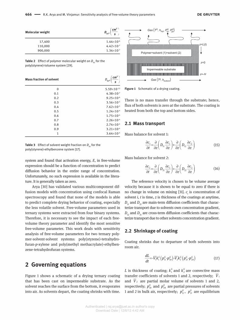
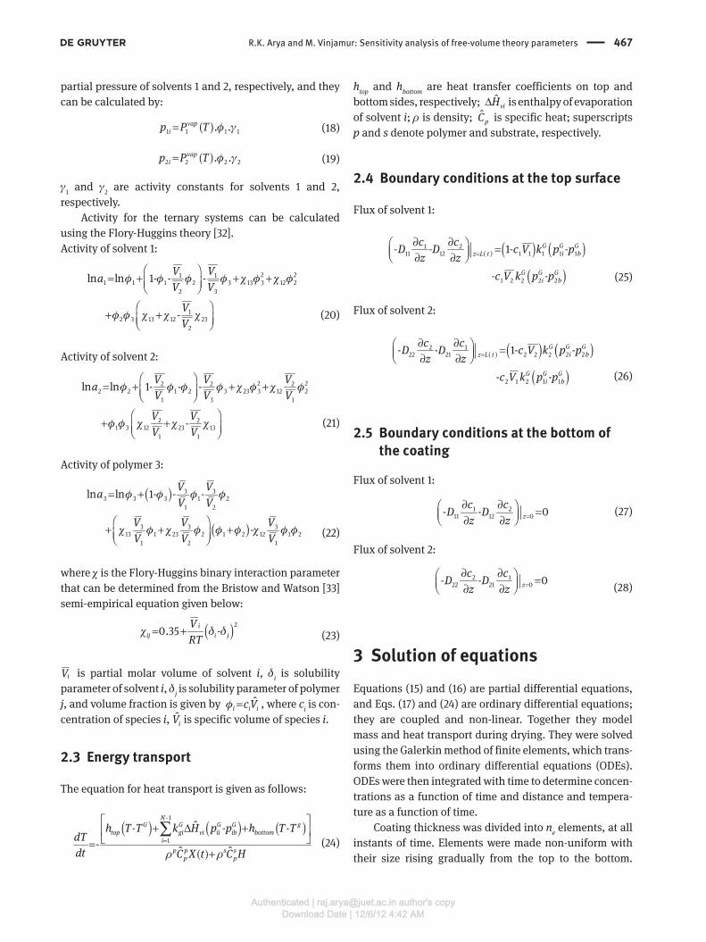
2 Governing equations Figure 1 shows a schematic of a drying ternary coating

that has been cast on impermeable substrate. As the

solvent reaches the surface from the bottom, it evaporates

into air. As solvents depart, the coating shrinks with time.

There is no mass transfer through the substrate; hence,

flux of both solvents is zero at the substrate. The coating is

heated from both the top and bottom sides.

2.1 Mass transport

Mass balance for solvent 1:

1 1 211 12

∂ ∂ ∂ ∂ ∂⎛ ⎞ ⎛ ⎞= +⎜ ⎟ ⎜ ⎟⎝ ⎠ ⎝ ⎠∂ ∂ ∂ ∂ ∂c c c

D Dt z z z z

(15)

Mass balance for solvent 2:

2 1 221 22

∂ ∂ ∂ ∂ ∂⎛ ⎞ ⎛ ⎞= +⎜ ⎟ ⎜ ⎟⎝ ⎠ ⎝ ⎠∂ ∂ ∂ ∂ ∂c c c

D Dt z z z z

(16)

The reference velocity is chosen to be volume average

velocity because it is shown to be equal to zero if there is

no change in volume on mixing [31] . c i is concentration of

solvent i , t is time, z is thickness of the coatings at anytime,

D 11 and D

22 are main-term diffusion coefficients that charac-

terize transport due to solvents own concentration gradient,

D 12

and D 21

are cross-term diffusion coefficients that charac-

terize transport due to other solvents concentration gradient.

2.2 Shrinkage of coating

Coating shrinks due to departure of both solvents into

room air.

( ) ( )1 1 1 1 2 2 2 2- - - -= G G G G G G

i b i b

dLV k p p V k p p

dt (17)

L is thickness of coating; kG

1 and kG

2 are convective mass

transfer coefficients of solvents 1 and 2, respectively; 1V

and 2V are partial molar volume of solvents 1 and 2,

respectively; 1

G

bp and 2

G

bp are partial pressures of solvents

1 and 2 in bulk air, respectively; 1

G

ip , 2

G

ip are equilibrium

Molecular weight D 01 , ⎛ ⎞⎜ ⎟⎝ ⎠cms

2

17,400 1.44 × 10 -6

110,000 4.42 × 10 -7

900,000 1.34 × 10 -7

Table 2 Effect of polymer molecular weight on D 01

for the

poly(styrene)-toluene system [29] .

Mass fraction of solvent D 01 , ⎛ ⎞

⎜ ⎟⎝ ⎠cms

2

0 5.59 × 10 -13

0.1 4.38 × 10 -7

0.2 9.25 × 10 -6

0.3 3.56 × 10 -5

0.4 7.62 × 10 -5

0.5 1.24 × 10 -4

0.6 1.75 × 10 -4

0.7 2.26 × 10 -4

0.8 2.74 × 10 -4

0.9 3.21 × 10 -4

1 3.64 × 10 -4

Table 3 Effect of solvent weight fraction on D 01

for the

poly(styrene)-ethylbenzene system [17] .

Polymer+solvent (1)+solvent (2)

z=L(t)

z=-H

z=0

Impermeable substrate

Gas (TG, htop, PG, PG)2b1b

Gas (Tg, hbottom)

Figure 1 Schematic of a drying coating.



partial pressure of solvents 1 and 2, respectively, and they

can be calculated by:

( )1 1 1 1. .= vap

ip P T φ γ (18)

( )2 2 2 2. .= vap

ip P T φ γ (19)

γ 1 and γ

2 are activity constants for solvents 1 and 2,

respectively.

Activity for the ternary systems can be calculated

using the Flory-Huggins theory [32] .

Activity of solvent 1:

2 21 11 1 1 2 3 13 3 12 2

2 3

12 3 13 12 23

2

ln ln 1- - -

-

V Va

V V

V

V

φ φ φ φ χ φ χ φ

φ φ χ χ χ

⎛ ⎞= + + +⎜ ⎟⎝ ⎠

⎛ ⎞+ +⎜ ⎟⎝ ⎠

(20)

Activity of solvent 2:

2 22 2 22 2 1 2 3 23 3 12 2

1 3 1

2 21 3 12 23 13

1 1

ln ln 1- - -

-

V V Va

V V V

V V

V V

φ φ φ φ χ φ χ φ

φ φ χ χ χ

⎛ ⎞= + + +⎜ ⎟⎝ ⎠

⎛ ⎞+ +⎜ ⎟⎝ ⎠

(21)

Activity of polymer 3:

( )

( )

3 33 3 3 1 2

1 2

3 3 313 1 23 2 1 2 12 1 2

1 2 1

ln ln 1- - -

-

V Va

V V

V V V

V V V

φ φ φ φ

χ φ χ φ φ φ χ φ φ

= +

⎛ ⎞+ + +⎜ ⎟⎝ ⎠ (22)

where χ is the Flory-Huggins binary interaction parameter

that can be determined from the Bristow and Watson [33]

semi-empirical equation given below:

( )2

0.35 -= + i

ij i j

V

RTχ δ δ

(23)

iV is partial molar volume of solvent i , δ i is solubility

parameter of solvent i , δ j is solubility parameter of polymer

j , and volume fraction is given by ˆ=i i ic Vφ , where c i is con-

centration of species i , ̂ iV is specific volume of species i .

2.3 Energy transport

The equation for heat transport is given as follows:

( ) ( ) ( )( )

-1

1

ˆ- - -

-ˆ ˆ

NG G G G g

top gi vi ii ib bottom

i

p p s s

p p

h T T k H p p h T TdT

dt C X t C Hρ ρ=

⎡ ⎤+ Δ +⎢ ⎥

⎣ ⎦=+

∑

(24)

h top

and h bottom

are heat transfer coefficients on top and

bottom sides, respectively; ˆΔ viH is enthalpy of evaporation

of solvent i ; ρ is density; ˆpC is specific heat; superscripts

p and s denote polymer and substrate, respectively.

2.4 Boundary conditions at the top surface

Flux of solvent 1:

( ) ( )( )

1 211 12 1 1 1 1 1( )

1 2 2 2 2

- - 1- -

- -

G G G

i bz L t

G G G

i b

c cD D c V k p p

z z

c V k p p

=∂ ∂⎛ ⎞ =⎜ ⎟⎝ ⎠∂ ∂

(25)

Flux of solvent 2:

( ) ( )( )

2 122 21 2 2 2 2 2( )

2 1 2 1 1

- - 1- -

- -

G G G

i bz L t

G G G

i b

c cD D c V k p p

z z

c V k p p

=∂ ∂⎛ ⎞ =⎜ ⎟⎝ ⎠∂ ∂

(26)

2.5 Boundary conditions at the bottom of the coating

Flux of solvent 1:

1 211 12 0- - 0=

∂ ∂⎛ ⎞ =⎜ ⎟⎝ ⎠∂ ∂ z

c cD D

z z

(27)

Flux of solvent 2:

2 122 21 0- - 0=

∂ ∂⎛ ⎞ =⎜ ⎟⎝ ⎠∂ ∂ z

c cD D

z z

(28)

3 Solution of equations Equations (15) and (16) are partial differential equations,

and Eqs. (17) and (24) are ordinary differential equations;

they are coupled and non-linear. Together they model

mass and heat transport during drying. They were solved

using the Galerkin method of finite elements, which trans-

forms them into ordinary differential equations (ODEs).

ODEs were then integrated with time to determine concen-

trations as a function of time and distance and tempera-

ture as a function of time.

Coating thickness was divided into n e elements, at all

instants of time. Elements were made non-uniform with

their size rising gradually from the top to the bottom.



Elements near the top were chosen to be small to capture

the precipitous drop in concentration there. A benefit of

using non-uniform elements is reduction in computation

time. A function,

2

-1⎛ ⎞=⎜ ⎟⎝ ⎠i

e

ir L

n, where i varies from 1 to n

e + 1

stretched the elements from the top to the bottom of the

coating. The size of element i can be obtained by r i + 1

- r i .

The exponent in the stretching function can be changed

to raise or lower stretching. The set of ODEs generated

was integrated by a stiff solver, ode15s , of MATLAB (The

MathWorks, Inc., Natick, MA, USA). A typical run on a

2.66 GHz computer with a memory of 506 Mbytes takes

approximately 20 s. The code was tested with the pub-

lished results of Alsoy and Duda [13] .

4 Estimation of free-volume parameters

The four free-volume parameters were estimated along

the same lines as Price et al. [26] . A code for drying of

binary polymer-solvent systems was written and used to

generate residual solvent as a function of time. Weight

loss data were collected for four polymer-solvent pairs,

poly(styrene)-tetrahydrofuran, poly(styrene)- p -xylene,

poly(methyl methacrylate)-ethylbenzene and poly

(methyl methacrylate)-tetrahydrofuran at room tempera-

ture and quiescent conditions. The difference between

experimental and predicted residual solvents, defined

here as an objective function, was minimized by using a

built-in optimization code, lsqnonlin , of MATLAB. Arya

[30] compared experiments and model predictions with

optimized values and free-volume parameters for his case

are listed in Table 4 for the four pairs.

5 Results and discussion Multiple sets of the four parameters estimated, for the

two systems, could minimize the objective function (dif-

ference between predicted and experimental weight loss

data). Hence, a sensitivity analysis was made for the poly

(styrene)- p -xylene-tetrahydrofuran system by chang-

ing the four parameters. Also, sensitivity with respect

to mass and heat transfer coefficients was studied. To

shorten the length of the paper, detailed analyses of the

poly(styrene)- p -xylene-tetrahydrofuran system are given,

whereas only final results in tabular form are given for the

poly(methyl methacrylate)-ethylbenzene-tetrahydrofuran

system. A less volatile solvent ( p -xylene, ethylbenzene),

a high volatile solvent (tetrahydrofuran) and a polymer,

poly(styrene), poly(methyl methacrylate) are referred

to as 1, 2 and 3, respectively. Initial concentrations of

poly(styrene), tetrahydrofuran and p -xylene were 0.128,

0.632 and 0.141 g cm -3 , respectively, initial coating thick-

ness was 1004 μ m and initial temperatures of coating and

Parameter Unit PS (3)/THF (2) PS(3)/ p -xylene (1) PMMA (3)/THF (2) PMMA (3)/EB (1)

D 0

2cm

s 97.99 ×× 10 -4 78.44 ×× 10 -4 98.75 ×× 10 -4 4.11 ×× 10 -4

γ13K

3cm

g.K 2.89 ×× 10 -4 2.89 ×× 10 -4 5.89 ×× 10 -4 5.89 ×× 10 -4

K 23

K -326.46 -326.46 -230.44 -230.44

ξ 0.38 0.44 0.65 0.30

K 2 i K 10.45 41.65 10.45 -80.01

γ1tK

3cm

g.K7.53 ×× 10 -4 7.6 ×× 10 -4 7.53 ×× 10 -4 2.22 ×× 10 -3

ˆ*

iV cm 3 g -1 0.899 1.049 0.899 0.946

ˆ*

3V cm 3 g -1 0.855 0.855 0.788 0.788

χ i 3 0.3652 0.5429 0.3925 0.3501

χ 12

0.4371 0.4371 0.4188 0.4188

Table 4 Free-volume parameters of four binary polymer solvent systems.

The values shown in bold font were obtained from optimization. The values of other parameters were obtained from Hong [20] . Solvents properties/coefficients : enthalpy of vaporization of tetrahydrofuran = 413.53 J g -1 ; enthalpy of vaporization of p -xylene = 335.98 J g -1 ;

enthalpy of vaporization of ethylbenzene = 335.03 J g -1 ; mass transfer coefficient of tetrahydrofuran = 1.74 × 10 -9 s cm -1 ; mass transfer

coefficient of p -xylene = 1.92 × 10 -9 s cm -1 . Substrate properties : thickness of sample holder = 0.15 cm; density of sample holder = 8 g cm -3 ;

specific heat capacity of substrate = 0.5 J g -1 K -1 ; thermal conductivity of substrate = 0.162 W cm -1 K -1 . Polymer properties : specific heat

capacity of poly(styrene) = 1.17 J g -1 K -1 ; specific heat capacity of poly(methyl methacrylate) = 1.5 J g -1 K -1 .



air were 23 ° C. Initial concentrations of poly(methyl meth-

acrylate), tetrahydrofuran and ethylbenzene were 0.216,

0.600 and 0.122 g cm -3 , respectively, initial coating thick-

ness was 983 μ m and initial temperatures of coating and

air were 23 ° C.

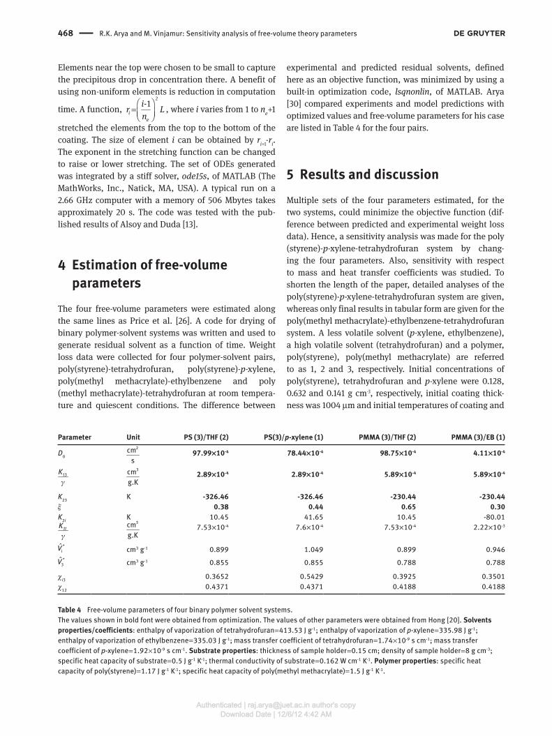
5.1 Effect of D 01 and D 02

Raising pre-exponential factors increases diffusion coef-

ficients. Figures 2 and 3 show that the predictions of

concentration of p -xylene are more sensitive than those

of tetrahydrofuran and poly(styrene) when the pre-expo-

nential factor for tetrahydrofuran, D 02

, was changed from

its optimal value by ± 5 % . Lowering D 02

reduces rate of

removal of tetrahydrofuran and its concentration gradi-

ent is expected to develop slowly. Hence, contribution

of cross-term to mass transfer of p -xylene reduces and

its concentration falls slowly. A similar effect was found

when D 01

, the pre-exponential factor for p -xylene, was

raised. Hong [20] also observed the same effect in the case

of binary systems.

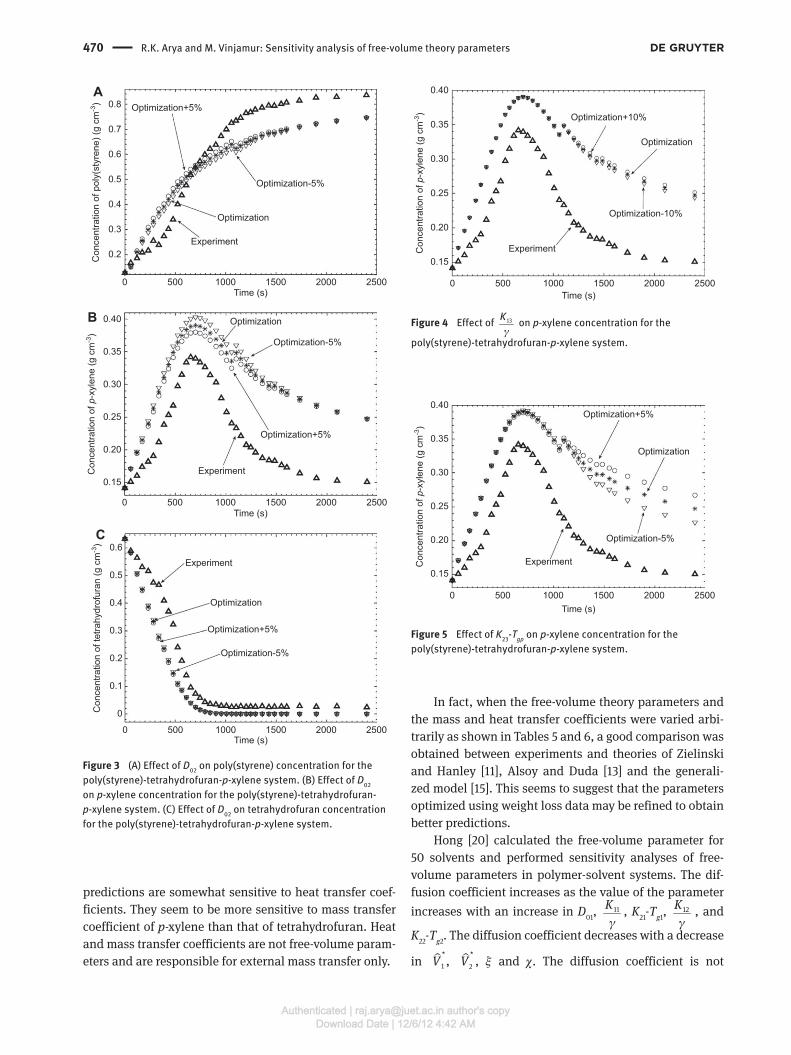
5.2 Effect of and K 23 - T gp

Raising 13K

γ and/or K

23 - T

gp increases the hole free-volume

available for diffusion and hence diffusion coefficients.

Figures 4 and 5 show that predictions are insensitive to

changes in 13K

γ. A small rise in K

23 - T

gp , however, rises the

concentrations of p -xylene from those predicted by opti-

mized values. Hong [20] has also found out that these

parameters are more sensitive at solvent weight fraction

equal to 0.1 and become less sensitive at higher concen-

trations in the case of binary systems. Ternary results

reported here are similar to Hong [20] .

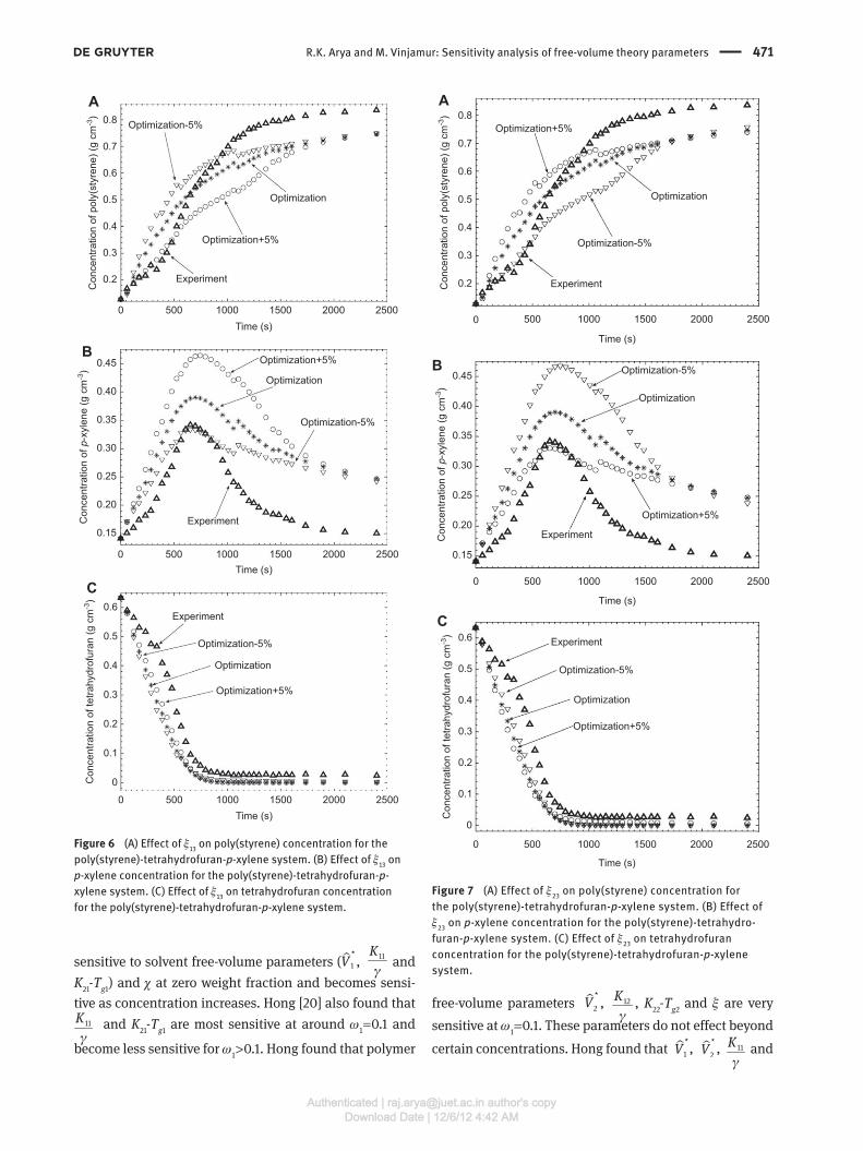
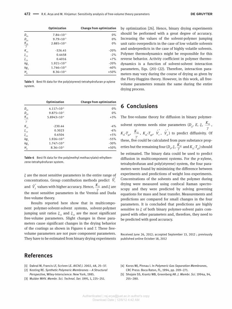
5.3 Effect of ξ 13 and ξ 23

Raising ξ 13

and/or lowering ξ 23

rises free volume required

for diffusion for tetrahydrofuran and lowers it for p -xylene.

Hence, self-diffusion coefficient of tetrahydrofuran would

be lowered and that of p -xylene would be raised. Figures 6

and 7 show that concentrations of tetrahydrofuran would

be lower and those of p -xylene would be higher than those

predicted by their optimized values if ξ 13

is lowered by 5 % .

The same effect is found when ξ 23

is raised by 5 % . These

are two parameters which significantly affect concentra-

tion. Hong [20] also observed the same effect in the case

of binary systems.

0.2

0 500 1000 1500Time (s)

Experiment

Experiment

Experiment

Optimization

Optimization

Optimization

Optimization+5%

Optimization+5%

Optimization-5%

Optimization+5%

Optimization-5%

Optimization-5%

Con

cent

ratio

n of

pol

y(st

yren

e) (g

cm

-3)

Con

cent

ratio

n of

p-x

ylen

e (g

cm

-3)

25002000

0 500 1000 1500Time (s)

25002000

0 500 1000 1500Time (s)

25002000

0.3

0.4

0.20

0.25

0.15

0.30

0.35

0.40

Con

cent

ratio

n of

tetra

hydr

ofur

an (g

cm

-3) 0.6

0.5

0.4

0.3

0.2

0.1

0

0.5

0.6

0.7

0.8A

B

C

Figure 2 (A) Effect of D 01

on poly(styrene) concentration for the

poly(styrene)-tetrahydrofuran- p -xylene system. (B) Effect of D 01

on

p -xylene concentration for the poly(styrene)-tetrahydrofuran- p -

xylene system. (C) Effect of D 01

on tetrahydrofuran concentration

for the poly(styrene)-tetrahydrofuran- p -xylene system.

5.4 Effect of heat and mass transfer coefficients

Mass and heat transfer coefficients were varied because it

is not uncommon for them to vary over a large range. The



0.2

0 500 1000 1500Time (s)

Experiment

Experiment

Experiment

Optimization

Optimization

Optimization

Optimization-5%

Optimization-5%

Optimization-5%

Optimization+5%

Optimization+5%

Optimization+5%

Con

cent

ratio

n of

pol

y(st

yren

e) (g

cm

-3)

25002000

0 500 1000 1500Time (s)

25002000

0 500 1000 1500Time (s)

25002000

0.3

0.4

0.5

0.6

0.7

0.8A

Con

cent

ratio

n of

p-x

ylen

e (g

cm

-3)

0.20

0.25

0.15

0.30

0.35

0.40B

Con

cent

ratio

n of

tetra

hydr

ofur

an (g

cm

-3) 0.6

0.5

0.4

0.3

0.2

0.1

0

C

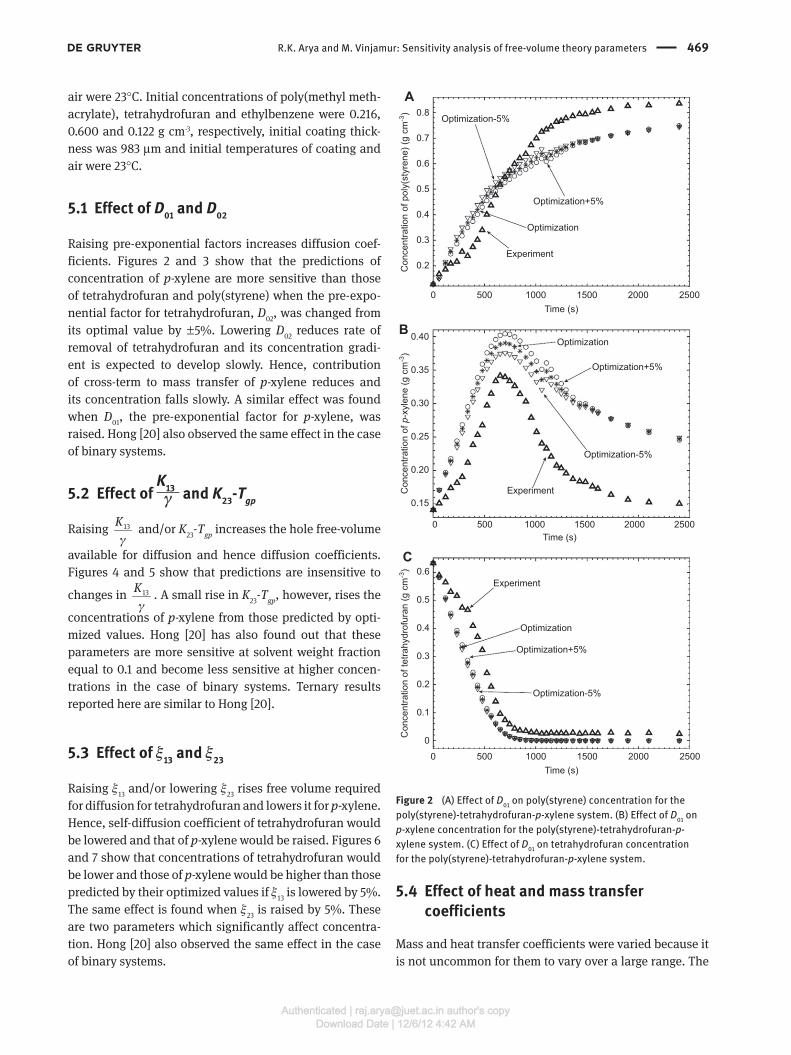
Figure 3 (A) Effect of D 02


poly(styrene)-tetrahydrofuran- p -xylene system. (B) Effect of D 02

on p -xylene concentration for the poly(styrene)-tetrahydrofuran-

p -xylene system. (C) Effect of D 02



Experiment

Optimization

Optimization+10%

Optimization-10%

Con

cent

ratio

n of

p-x

ylen

e (g

cm

-3)

0 500 1000 1500Time (s)

25002000

0.20

0.25

0.15

0.30

0.35

0.40

Figure 4 Effect of 13

γK

on p -xylene concentration for the

poly(styrene)-tetrahydrofuran- p -xylene system.

Experiment

Optimization

Optimization+5%

Optimization-5%

Con

cent

ratio

n of

p-x

ylen

e (g

cm

-3)

0 500 1000 1500Time (s)

25002000

0.20

0.25

0.15

0.30

0.35

0.40

Figure 5 Effect of K 23

- T gp on p -xylene concentration for the

poly(styrene)-tetrahydrofuran- p -xylene system.

predictions are somewhat sensitive to heat transfer coef-

ficients. They seem to be more sensitive to mass transfer

coefficient of p -xylene than that of tetrahydrofuran. Heat

and mass transfer coefficients are not free-volume param-

eters and are responsible for external mass transfer only.

In fact, when the free-volume theory parameters and

the mass and heat transfer coefficients were varied arbi-

trarily as shown in Tables 5 and 6 , a good comparison was

obtained between experiments and theories of Zielinski

and Hanley [11] , Alsoy and Duda [13] and the generali-

zed model [15] . This seems to suggest that the parameters

optimized using weight loss data may be refined to obtain

better predictions.

Hong [20] calculated the free-volume parameter for

50 solvents and performed sensitivity analyses of free-

volume parameters in polymer-solvent systems. The dif-

fusion coefficient increases as the value of the parameter

increases with an increase in D 01

, 11K

γ, K

21 - T

g 1 , 12K

γ, and

K 22

- T g 2 . The diffusion coefficient decreases with a decrease

in �*

1V , �*

2V , ξ and χ . The diffusion coefficient is not



0.2

0 500 1000 1500Time (s)

Experiment

Optimization

Optimization-5%

Optimization+5%

Con

cent

ratio

n of

pol

y(st

yren

e) (g

cm

-3)

25002000

0.3

0.4

0.5

0.6

0.7

0.8A

Experiment

Optimization

Optimization+5%

Optimization-5%

Con

cent

ratio

n of

p-x

ylen

e (g

cm

-3)

0 500 1000 1500Time (s)

25002000

0.20

0.25

0.15

0.30

0.35

0.45

0.40

B

Experiment

Optimization

Optimization-5%

Optimization+5%

0 500 1000 1500Time (s)

25002000

Con

cent

ratio

n of

tetra

hydr

ofur

an (g

cm

-3)

0.6

0.5

0.4

0.3

0.2

0.1

0

C

Figure 6 (A) Effect of ξ 13


poly(styrene)-tetrahydrofuran- p -xylene system. (B) Effect of ξ 13

on

p -xylene concentration for the poly(styrene)-tetrahydrofuran- p -

xylene system. (C) Effect of ξ 13



Experiment

Optimization

Optimization+5%

Optimization-5%

0 500 1000 1500

Time (s)

25002000

Con

cent

ratio

n of

tetra

hydr

ofur

an (g

cm

-3) 0.6

0.5

0.4

0.3

0.2

0.1

0

C

Experiment

Optimization

Optimization+5%

Optimization-5%

Con

cent

ratio

n of

p-x

ylen

e (g

cm

-3)

0 500 1000 1500

Time (s)

25002000

0.20

0.25

0.15

0.30

0.35

0.40

0.45B

0.2

0 500 1000 1500

Time (s)

Experiment

Optimization

Optimization-5%

Optimization+5%

Con

cent

ratio

n of

pol

y(st

yren

e) (g

cm

-3)

25002000

0.3

0.4

0.5

0.6

0.7

0.8A

Figure 7 (A) Effect of ξ 23

on poly(styrene) concentration for

the poly(styrene)-tetrahydrofuran- p -xylene system. (B) Effect of

ξ 23

on p -xylene concentration for the poly(styrene)-tetrahydro-

furan- p -xylene system. (C) Effect of ξ 23

on tetrahydrofuran

concentration for the poly(styrene)-tetrahydrofuran- p -xylene

system. sensitive to solvent free-volume parameters ( �

*

1V , 11K

γ and

K 21

- T g 1 ) and χ at zero weight fraction and becomes sensi-

tive as concentration increases. Hong [20] also found that

11K

γ and K

21 - T

g 1 are most sensitive at around ω

1 = 0.1 and

become less sensitive for ω 1 > 0.1. Hong found that polymer

free-volume parameters �*

2V ,

12K

γ, K

22 - T

g 2 and ξ are very

sensitive at ω 1 = 0.1. These parameters do not effect beyond

certain concentrations. Hong found that �*

1V , �*

2V , 11K

γ and



ξ are the most sensitive parameters in the entire range of

concentrations. Group contribution methods predict �*

1V

and �*

2V values with higher accuracy. Hence, 11K

γ and ξ are

the most sensitive parameters in the Vrentas and Duda

free-volume theory.

Results reported here show that in multicompo-

nent polymer-solvent-solvent systems, solvent-polymer

jumping unit ratios ξ 13

and ξ 23

are the most significant

free-volume parameters. Slight changes in these para-

meters cause significant changes in the drying behavior

of the coatings as shown in Figures 6 and 7. These free-

volume parameters are not pure component parameters.

They have to be estimated from binary drying experiments

by optimization [26] . Hence, binary drying experiments

should be performed with a great degree of accuracy.

Increasing the values of the solvent-polymer jumping

unit ratio overpredicts in the case of low volatile solvents

and underpredicts in the case of highly volatile solvents.

Polymer thermodynamics might be responsible for this

reverse behavior. Activity coefficient in polymer thermo-

dynamics is a function of solvent-solvent interaction

parameters, Eqs. (20) – (22). Therefore, interaction para-

meters may vary during the course of drying as given by

the Flory-Huggins theory. However, in this work, all free-

volume parameters remain the same during the entire

drying process.

6 Conclusions The free-volume theory for diffusion in binary polymer-

solvent systems needs nine parameters ( D 0 , E , ξ , 11K

γ,

K 21

- T gs

, 12K

γ, K

22 - T

gp ,

*^

sV ,

*^

pV ) to predict diffusivity. Of

these, five could be calculated from pure substance prop-

erties but the remaining four ( D 0 , ξ ,

12K

γ and K 22

- T g 2 ) should

be estimated. The binary data could be used to predict

diffusion in multicomponent systems. For the p- xylene,

tetrahydrofuran and poly(styrene) system, the four para-

meters were found by minimizing the difference between

experiments and predictions of weight loss experiments.

Concentrations of the solvents and the polymer during

drying were measured using confocal Raman spectro-

scopy and they were predicted by solving governing

equations for mass and heat transfer. Measurements and

predictions are compared for small changes in the four

parameters. It is concluded that predictions are highly

sensitive to ξ of both binary polymer-solvent pairs com-

pared with other parameters and, therefore, they need to

be predicted with good accuracy.

Received June 26, 2012; accepted September 13, 2012 ; previously

published online October 18, 2012

References [1] Dabral M, Francis LF, Scriven LE. AIChE J. 2002, 48, 25 – 37.

[2] Kesting RE. Synthetic Polymeric Membranes – A Structural Perspective , Wiley-Interscience: New York, 1985.

[3] Mulder MHV. Membr. Sci. Technol. Ser. 1991, 1, 225 – 251.

[4] Koros WJ, Pinnau I. In Polymeric Gas Separation Membranes ,

CRC Press: Boca Raton, FL, 1994, pp. 209 – 271.

[5] Shojaie SS, Krantz WB, Greenberg AR. J. Membr. Sci. 1994a, 94,

255 – 280.

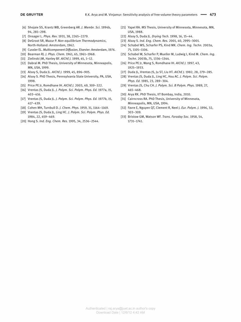
Optimization Change from optimization

D 01

7.84 × 10 -3 0 %

D 01

9.79 × 10 -3 0 %

γK13 2.885 × 10 -4 0 %

K 23

-326.45 -20 %

ξ 13

0.4458 -2 %

ξ 23

0.4016 + 7 %

kg 1 1.921 × 10 -9 -20 %

kg 2 1.746 × 10 -9 -40 %

H G 8.36 × 10 -4 + 50 %

Table 5 Best fit data for the poly(styrene)-tetrahydrofuran- p -xylene

system.

Optimization Change from optimization

D 01

4.117 × 10 -4 0 %

D 02

9.875 × 10 -3 0 %

γK13 5.8943 × 10 -4 + 3 %

K 23

-230.44 -4 %

ξ 13

0.3023 -6 %

ξ 23

0.6504 + 5 %

kg 1 1.926 × 10 -9 -55 %

kg 2 1.747 × 10 -9 -30 %

H G 8.36 × 10 -4 + 50 %

Table 6 Best fit data for the poly(methyl methacrylate)-ethylben-

zene-tetrahydrofuran system.



[6] Shojaie SS, Krantz WB, Greenberg AR. J. Membr. Sci. 1994b,

94, 281 – 298.

[7] Onsager L. Phys. Rev. 1931, 38, 2265 – 2279.

[8] DeGroot SR, Mazur P. Non-equilibrium Thermodynamics ,

North-Holland: Amsterdam, 1962.

[9] Cussler EL. Multicomponent Diffusion , Elsevier: Amsterdam, 1976.

[10] Bearman RJ. J. Phys. Chem. 1961, 65, 1961 – 1968.

[11] Zielinski JM, Hanley BF. AIChE J. 1999, 45, 1 – 12.

[12] Dabral M. PhD Thesis, University of Minnesota, Minneapolis,

MN, USA, 1999.

[13] Alsoy S, Duda JL. AIChE J. 1999, 45, 896 – 905.

[14] Alsoy S. PhD Thesis, Pennsylvania State University, PA, USA,

1998.

[15] Price PE Jr, Romdhane IH. AIChE J. 2003, 49, 309 – 322.

[16] Vrentas JS, Duda JL. J. Polym. Sci. Polym. Phys. Ed. 1977a, 15,

403 – 416.

[17] Vrentas JS, Duda JL. J. Polym. Sci. Polym. Phys. Ed. 1977b, 15,

417 – 439.

[18] Cohen MH, Turnbull D. J. Chem. Phys. 1959, 31, 1164 – 1169.

[19] Vrentas JS, Duda JL, Ling HC. J. Polym. Sci. Polym. Phys. Ed. 1984, 22, 459 – 469.

[20] Hong S. Ind. Eng. Chem. Res. 1995, 34, 2536 – 2544.

[21] Yapel RA. MS Thesis, University of Minnesota, Minnesota, MN,

USA, 1988.

[22] Alsoy S, Duda JL. Drying Tech. 1998, 16, 15 – 44.

[23] Alsoy S. Ind. Eng. Chem. Res. 2001, 40, 2995 – 3001.

[24] Schabel WS, Scharfer PS, Kind MK. Chem. Ing. Techn. 2003a,

75, 1105 – 1106.

[25] Schabel W, Scharfer P, Mueller M, Ludwig I, Kind M. Chem. Ing. Techn. 2003b, 75, 1336 – 1344.

[26] Price PE Jr, Wang S, Romdhane IH. AIChE J. 1997, 43,

1925 – 1933.

[27] Duda JL, Vrentas JS, Ju ST, Liu HT. AIChE J. 1982, 28, 279 – 285.

[28] Vrentas JS, Duda JL, Ling HC, Hou AC. J. Polym. Sci. Polym. Phys. Ed. 1985, 23, 289 – 304.

[29] Vrentas JS, Chu CH. J. Polym. Sci. B Polym. Phys. 1989, 27,

465 – 468.

[30] Arya RK. PhD Thesis, IIT Bombay, India, 2010.

[31] Cairncross RA. PhD Thesis, University of Minnesota,

Minneapolis, MN, USA, 1994.

[32] Favre E, Nguyen QT, Clement R, Neel J. Eur. Polym. J. 1996, 32,

303 – 309.

[33] Bristow GM, Watson WF. Trans. Faraday Soc. 1958, 54,

1731 – 1741.


Documents

Sensitivity analysis of free-volume theory parameters in multicomponent polymer-solvent-solvent systems