Embed Size (px)
Citation preview

This article appeared in a journal published by Elsevier. The attachedcopy is furnished to the author for internal non-commercial researchand education use, including for instruction at the authors institution
and sharing with colleagues.
Other uses, including reproduction and distribution, or selling orlicensing copies, or posting to personal, institutional or third party
websites are prohibited.
In most cases authors are permitted to post their version of thearticle (e.g. in Word or Tex form) to their personal website orinstitutional repository. Authors requiring further information
regarding Elsevier’s archiving and manuscript policies areencouraged to visit:
http://www.elsevier.com/authorsrights

Author's personal copy
Sensitivity of direct canopy gap fraction retrieval from airbornewaveform lidar to topography and survey characteristics☆
X.T. Chen a, M.I. Disney b,c,⁎, P. Lewis b,c, J. Armston d,e, J.T. Han a, J.C. Li a
a College of Electronic Science and Engineering, National University of Defense Technology, 137 Yanwachi, Changsha, Hunan 410073, PR Chinab Dept. of Geography, University College London, Gower Street, London WC1E 6BT, UKc NERC National Centre for Earth Observation (NCEO), UKd Remote Sensing Centre, Science Delivery, Department of Science, Information Technology, Innovation and the Arts, 41 Boggo Road, QLD 4102, Australiae Joint Remote Sensing Research Program, School of Geography, Planning and Environmental Management, University of Queensland, St Lucia, QLD 4072, Australia
a b s t r a c ta r t i c l e i n f o
Article history:Received 30 September 2013Received in revised form 16 December 2013Accepted 17 December 2013Available online 15 January 2014
Keywords:Waveform lidarCanopyGap fractionAirborneForestBiophysical parameters
Recently, Armston et al. (2013) have demonstrated that a new, physically-based method for direct retrieval ofcanopy gap probability Pgap from waveform lidar can improve the estimation of Pgap over discrete return lidardata. The success of the approach was demonstrated in a savanna woodland environment in Australia. Thehuge advantage of this method is that it uses the data themselves to solve for the canopy contrast term i.e. theratio of the reflectance from crown and ground, ρv/ρg. In this way the method avoids local calibration that istypically required to overcome differences in either ρv or ρg. To be more generally useful the method must bedemonstrated on different sites and in the presence of slope and different sensor and survey configurations. Ifit is robust to these things, slope in particular, then we would suggest it is likely to be widely useful. Here, wetest the robustness of the retrieval of Pgap fromwaveform lidar using theWatershedAllied Telemetry Experimen-tal Research dataset, over the Heihe River Basin region of China. The data contain significant canopy, terrain andsurvey variations, presenting a rather different set of conditions to those previously used. Results show that ρv/ρgis seen to be stable across all flights and for all levels of spatial aggregation. This strongly supports the robustnessof the new Pgap retrieval method, which assumes that this relationship is stable. A comparison between Pgap es-timated from hemiphotos and from the waveform lidar showed agreement with Pearson correlation coefficientR = 0.91. The waveform lidar-derived estimates of Pgap agreed to within 8% of values derived from hemiphotos,with a bias of 0.17%. The newwaveformmodel was shown to be stable across different off-nadir scan angles andin the presence of slopes up to 26°with R ≥ 0.85 in all cases.We also show that thewaveformmodel can be usedto calculate Pgap using just themean value of canopy returns, assuming that their distribution is unimodal. Lastly,we show that themethod can also be applied to discrete return lidar data, albeit with slightly lower accuracy andhigher bias, allowing Pgap comparisons with previously-collected lidar datasets. Our results show the newmeth-od should be applicable for estimating Pgap robustly across large areas, and from lidar data collected at differenttimes and using different systems; an increasingly important requirement.
© 2014 The Authors. Published by Elsevier Inc. All rights reserved.
1. Introduction
Directional gap probability, Pgap(θ), is defined as the probability of alight beam of infinitesimal width at zenith angle θ to the local normal,being directly transmitted through a vegetation canopy (Armstonet al., 2013). Pgap(θ), along with canopy height and leaf area index
(LAI), are some of the most important forest structural parametersused to directly interpret the transfer of radiation, carbon, and relatedprocesses in physical systems (Ross, 1981; Verstraete, Pinty, &Myneni, 1996). Pgap(θ) is equivalent to the probability that the groundsurface is directly visible from an airborne or spaceborne lidar remotesensing instrument. As a consequence, Pgap(θ) is a structural parameterthat may be near-directly retrieved from airborne lidar measurements(Ni-Meister, Jupp, & Dubayah, 2001).
The importance of Pgap(θ) is its relationship to radiation interceptionwithin the canopy and hence other canopy structure parameters, likeLAI and above-ground biomass (Campbell & Norman, 1989; Ni-Meister et al., 2010). These latter properties may be modelled usingdifferent expressions, combinations or spatial variance of canopy heightand Pgap(θ), since the Pgap(θ) represents the integrated effect of severalscale-dependent canopy structural properties (in particular LAI and leaf
Remote Sensing of Environment 143 (2014) 15–25
☆ This is an open-access article distributed under the terms of the Creative CommonsAttribution License, which permits unrestricted use, distribution, and reproduction in anymedium, provided the original author and source are credited.⁎ Corresponding author at: Dept. of Geography, University College London, Gower
Street, London WC1E 6BT, UK. Tel.: +44 20 7679 0592.E-mail addresses: [email protected] (X.T. Chen), [email protected]
(M.I. Disney), [email protected] (P. Lewis), [email protected](J. Armston), [email protected] (J.T. Han), [email protected] (J.C. Li).
0034-4257/$ – see front matter © 2014 The Authors. Published by Elsevier Inc. All rights reserved.http://dx.doi.org/10.1016/j.rse.2013.12.010
Contents lists available at ScienceDirect
Remote Sensing of Environment
j ourna l homepage: www.e lsev ie r .com/ locate / rse

Author's personal copy
angle distribution, LAD). In practice, Pgap(θ) is often calculated over anarrow range of angles e.g. close to nadir (θ = 0°) and is then referredto simply as Pgap. Here, we refer to Pgap and note where there may besome angular dependence.
Many studies have estimated Pgap or fractional cover (1- Pgap) usingsmall footprint discrete return lidar datesets (Hopkinson & Chasmer,2009; Liu et al., 2008; Lovell, Jupp, Culvenor, & Coops, 2003). Quantify-ing the proportion of lidar pulses intercepted by the canopy is themost common method to estimate the Pgap (Lovell et al., 2003). Thereare two problems in discrete return approaches to estimate Pgap(Armston et al., 2013): firstly, parameters estimated based on discretereturn lidar returns are only ‘effective’, i.e. they only have indirectcorrespondence with a physically-measurable estimate of the sameparameter whichmeans that they are difficult to validate and interpret;secondly, discrete return lidar approaches tend to rely on site-, sensor-and survey-specific calibrations, which limits the application of suchmethods in larger areas. In particular, topography and scan angle(as well as other things such as sensor flying height and even canopystructure and crown shape) combine in practice to modify the lidarreturn by changing the size and shape of the footprint and the pathlength through the canopy and hence the returned energy. These factorscan introduce significant bias into estimates of properties derived fromthe footprint, even in ‘simple’ metrics such as canopy height. Disneyet al. (2010) used detailed 3D Monte Carlo ray tracing to study theimpact of footprint size, scan angle and crown shape (among otherthings) on small footprint (b1 m) discrete return lidar estimates ofcanopy height, showing that these factors could lead to large over- orunderestimates depending on the situation. Yang, Ni-Meister, and Lee(2011) used a geometric-optics radiative transfer (GORT) model toexplore the impact of topography, crown shape and scan angle on largefootprint (N20 m) waveform lidar. They showed that the impact of to-pography and scan angle onwaveformproperties were similar and com-bined to smear out the returnedwaveform shape and reduce the energyreturnedwith height through the canopy, potentially resulting in canopyheight overestimates approaching 50%. Romanczyk et al. (2013) alsoshowed that the impact of within-crown distribution of leaf andwoody material on simulated waveform lidar returns varied withfootprint and scan angles. All of these effects will also impact esti-mates of Pgap, typically by acting to reduce it if the path lengththrough the canopy is increased by scan angle or topography (andvice versa).
Recently, a new method proposed by Armston et al. (2013) hasdemonstrated that a physically-based method for direct retrieval ofPgap from waveform lidar can improve the estimation of Pgap fromairborne platforms compared to discrete return lidar data in a savannawoodland environment. The method assumes that the ratio of thecanopy and ground reflectance characteristics, ρv and ρg respectively,is constant within a local area. The advantage of this method, is that ifρv/ρg is constant, then the method solves for the ratio term using thelidar waveforms themselves. Previous methods based on the propertiesof ρv/ρg have tended to require some estimate of either ρg or ρv toconstrain the ratio (e.g. Lefsky, Hudak, Cohen, & Acker, 2005). Hencethe method of Armston et al. (2013) does not rely on local calibrationthat is typically required to overcome differences in either ρv or ρg. Asa result it is less sensitive to possible changes in lidar system gain andinstrument altitude. This makes the method much more applicablefor large scale and/or repeat applications, where system and surveycharacteristics are very hard to replicate (or potentially even determine).
Armston et al. (2013) showed that the assumption of constant ρv/ρgheld very well for the cases they explored and produced estimates ofPgap corresponding to within 5% of ground measurements. They alsoshowed that the resulting Pgap estimates were relatively insensitive tovariations in sensor altitude, in contrast to other methods, where alti-tude variations can result in changes of up to 15% in estimated Pgap.
Crucially, if it can be demonstrated that the assumptions of stableρv/ρg holds across different sets of sensor, survey, and canopy structure
configurations than in the original study, and in contrasting environ-ments, this would provide further evidence that the method is moregenerally applicable. Additional validation of the method in differentenvironments is needed to demonstrate that a reduction or evenremoval of the requirements for local field calibration is justified,which in turn would advance the wider application of airborne wave-form lidar for estimating Pgap.
Here, we examine the physically-basedmethod for direct retrieval ofPgap from waveform lidar over a mountainous conifer forest region inthe Heihe River Basin region of China (Li et al., 2009). We use airbornewaveform lidar data containing a range of system variations (i.e. flyingheight, scanning angle, gain setting), over a survey area containing arange of different slopes and terrain types as well as a variation oftree type and density in a dense Picea forest environment (Tianet al., 2011). This extends validation of the stability of the assumptionof ρv/ρg to a new environment, containing significant topography, aswell as different canopy density and crown shape to those of Armstonet al. (2013). We also test the Pgap retrieval method using a discretereturn lidar dataset synthesised from the waveform data. This allowsus to test whether the physically-based Pgap estimation method couldalso be applied to discrete return data. If so, this would make itwidely-applicable to lidar datasets collected in the past with differentsensor systems. This would be of wide use in many lidar applications,particularly those examining changes over time i.e. comparing lidar-derived estimates of gap fraction over time.
2. Data
2.1. Study site and field data
In this study we use an airborne lidar survey comprising six flights,combined with forest structure parameter survey data to test theretrieval of Pgap. The lidar data were collected on 23/06/2008 over theDayekou watershed as part of the larger Watershed Allied TelemetryExperimental Research (WATER) project (Li et al., 2009).WATER coversthe Heihe River Basin in Northwest China, the second largest inlandriver basin in China, located between 37.68–42.70°N and 97.4–102.17°Ewith an area of about 130,000 km2. WATER is aimed at improving theunderstanding of physical processes of the land surface–atmosphere in-teraction in arid regions, and has resulted in the collection of simulta-neous airborne, satellite-borne remote sensing observations andground-based measurements. Fig. 1 shows the site location withinChina and a zoom on the map shows the coverage of the flight lines.
The so-called Dayekou Super Site is located at Xishui farm, Su'nanYuguzu Autonomous County in the Gansu Qilian Mountains NationalNature Reserve (38.53° N, 100.25° E). The site is a water resource con-servation forest in the Dayekou Basin of the Qilian Mountains, and lieswithin the temperate alpine, cold semiarid and semi-humid zones,characterized by mountain forest-steppe (Li et al., 2009). Sunny slopesare covered with mountain grassland, and shady slopes are forested.The elevation ranges from 2700 to 3000 m above sea level, with meanelevation of ~2800 m. Fig. 2 shows the topographic features of theSuper Site. There are four subplots in the test site (designated s1–s4).From the contours in Fig. 2, we see that s4 has the highest gradient atabout 15°. By contrast, s1 has the lowest gradient in all the subplots.The topographic variation here is more complex than the savannawoodland environment used in Armston et al. (2013), providing avery different set of conditions to test the assumptions underlying thePgap reconstruction method.
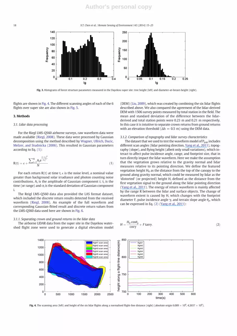
The forest cover across the Super Site is natural mature secondaryforest dominated by Picea crassifolia Kom, and the forestfloor is coveredmainly with moss (Carex lansuensis, Pedicularis muscicola, Polygonumviviparum). An inventory survey on the forest has been carried out inthe four subplots, including tree height (TH) and diameter at breastheight (DBH). Histograms of these forest structure parameters aregiven in Fig. 3 (Liu, 2009) .
16 X.T. Chen et al. / Remote Sensing of Environment 143 (2014) 15–25

Author's personal copy
From the histograms of DBH in Fig. 3 (and their kurtosis and skewnessparameters), it is clear that the smaller, less mature trees are morenumerous than the mature trees. From the bimodal characteristics ofthe histogram of TH it seems that there are distinct layers in the struc-ture of the forest canopy across the site. The higher part is composedof mature trees (N15 m), a lower part dominated by trees in the5–15 m range, and a bottom layer of young growth trees (b5 m).From Fig. 4 the forest structure here is denser and more mixed in age,and located on significant slopes in places, contrasting with that usedin Armston et al. (2013) which was dominated by sparse, maturetrees on flat surfaces.
2.2. Field data
Hemiphotos were taken looking upwards from the forest floor inthe supersite using a 180° fisheye lens (Canon EF15/28) and a highresolution digital camera (Canon EOS40D) (Chen & Guo, 2008; Chen,Guo, & Liu, 2008). The digital camera is mounted in a self-levelling
Mount, type SLM9. Hemiphotos were taken when the sky was evenlyovercast. 32 photographs taken from the subplots were analysed toprovide estimates of Pgap (plus variation) of each subplot, using theHemiView canopy image analysis system (Delta T Devices, Cambridge,UK). We obtained Pgap from Hemiphotos measuring the directionalgap probability at near-nadir i.e. zenith angles in the range 0–5°.
2.3. Lidar data
The lidar surveys used in this studywere acquired using a Riegl LMS-Q560 full waveform scanner during 6 flights over 23/06/2008. Details ofthe acquisitions are shown in Table 1 (Pang et al., 2008). Data wereacquired at flying heights of 700–750 m. The variation of elevationabove sea level between the flights was from 3500 to 3550 m. Parallelflight tracks were designed to have 90% overlap to ensure a multi-angular airborne dataset over the field sites and nearly nadir angular(b15°) scanning of the site. The coverage and nominal height of all
Yumen Jiayuguan Jiuquan
Jinta
Gaotai
LinzeZhangye
Shandan
Minle
Qilian
Su nan Yuguzu AutonomousCounty
Alasan
Jinchang
Yongchang
Fig. 1. Position sketch of Dayoukou Observation at water conversation forest in Qilian Mountain (source: Li et al., 2008) . The green box denotes the site of the lidar flights.
Fig. 2. Contours of the Dayoukou Super Site showing the locations of the subplots 1–4 using a local frame of reference (absolute origin 6.089 × 10⁶, 4.2657 × 10⁶).
17X.T. Chen et al. / Remote Sensing of Environment 143 (2014) 15–25
Author's personal copy
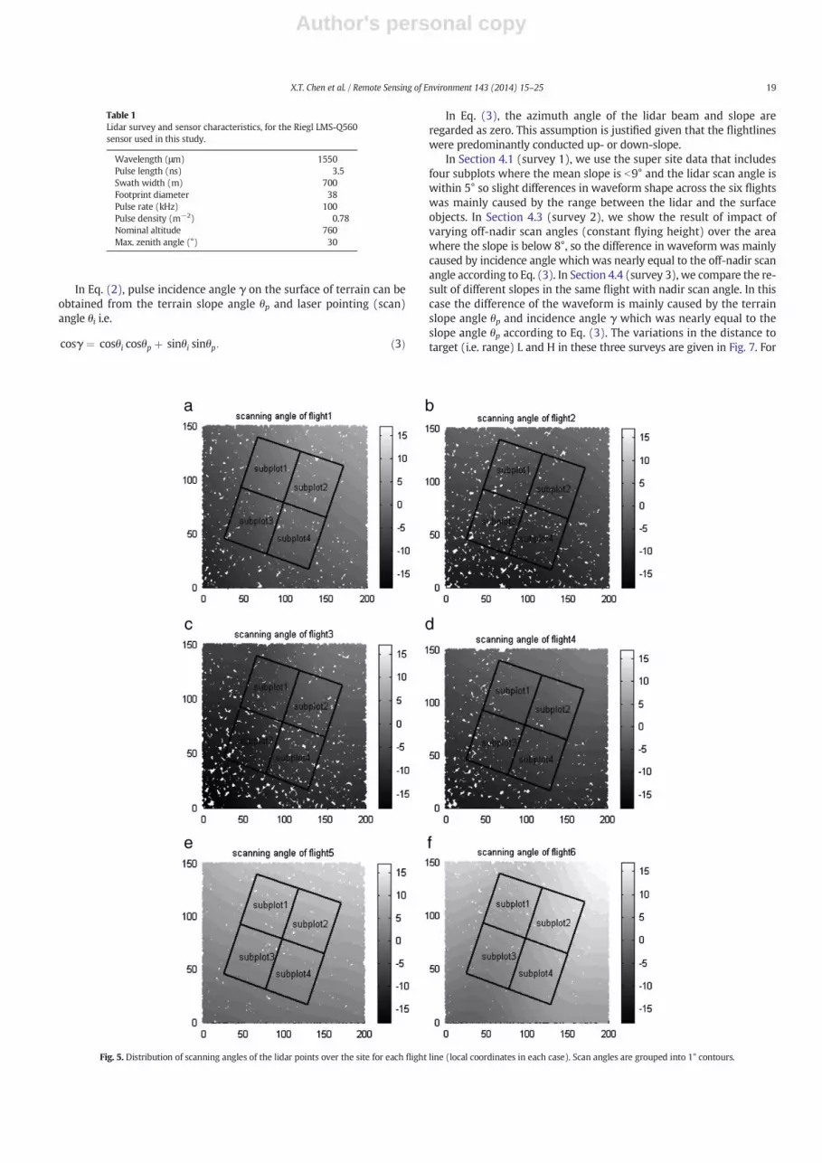
flights are shown in Fig. 4. The different scanning angles of each of the 6flights over super site are also shown in Fig. 5.
3. Methods
3.1. Lidar data processing
For the Riegl LMS-Q560 airborne surveys, raw waveform data weremade available (Riegl, 2008). These data were processed by Gaussiandecomposition using the method described by Wagner, Ullrich, Ducic,Melzer, and Studnicka (2006). This resulted in Gaussian parametersaccording to Eq. (1):
R tð Þ ¼ ϵ þXN
i¼1Aie
t−tið Þ22σi
2
Nð1Þ
For each return R(t) at time t, ϵ is the noise level, a nominal valuegreater than background solar irradiance and photon counting noisecontributions. Ai is the amplitude of Gaussian component i; ti is thetime (or range) and σi is the standard deviation of Gaussian componenti.
The Reigl LMS-Q560 data also provided the LAS format dataset,which included the discrete return results detected from the receivedwaveform (Riegl, 2008). An example of the full waveform andcorresponding Gaussian-fitted result and discrete return values fromthe LMS-Q560 data used here are shown in Fig. 6.
3.1.1. Separating crown and ground returns in the lidar dataThe airborne LIDAR data from the super site in the Dayekou water-
shed flight zone were used to generate a digital elevation model
(DEM) (Liu, 2009), whichwas created by combining the six lidar flightsdescribed above. We also compared the agreement of the lidar-derivedDEMwith 1506 survey pointsmeasured by total station in the field. Themean and standard deviation of the difference between the lidar-derived and total station points were 0.23 m and 0.21 m respectively.In this case it is intuitive to separate crown returns from ground returnswith an elevation threshold (Δh = 0.5 m) using the DEM data.
3.1.2. Comparison of topography and lidar survey characteristicsThedataset thatwe used to test thewaveformmodel of Pgap includes
different scan angles (lidar pointing direction, Yang et al., 2011), topog-raphy (slope), and flying height (albeit only small variations), which in-teract to affect pulse incidence angle, range, and footprint size, that inturn directly impact the lidar waveform. Here wemake the assumptionthat the vegetation grows relative to the gravity normal and lidarmeasures relative to its pointing direction. We define the featuredvegetation height H0 as the distance from the top of the canopy to theground along gravity normal, which could be measured by lidar as the‘distorted’ (or projected) height H, defined as the distance from thefirst vegetation signal to the ground along the lidar pointing direction(Yang et al., 2011). The energy of return waveform is mainly affectedby the range R between the lidar and surface objects. The change ofwaveform extent is caused by H, which changes with the footprintdiameter F, pulse incidence angle γ, and terrain slope angle θp, whichcan be expressed in Eq. (2) (Yang et al., 2011):
H ¼ H0 cosθpcosγ
þ F tanγ: ð2Þ
Fig. 3. Histograms of forest structure parameters measured in the Dayekou super site: tree height (left) and diameter-at-breast-height (right).
0 100 200 300 400 5000 500 1000 1500 2000 25000
600
400
200
800
1000
1200
1400
600700
750
800
850
time(s)
heig
ht a
long
a fl
ight
-line
dis
tanc
e(m
)
flight1flight2flight3flight4flight5flight6
flight1 scan areaflight2 scan areaflight3 scan areaflight4 scan areaflight5 scan areaflight6 scan area
Fig. 4. The scanning area (left) and height of the six lidar flights along a normalised flight-line distance (right) (absolute origin 6.089 × 10⁶, 4.2657 × 10⁶).
18 X.T. Chen et al. / Remote Sensing of Environment 143 (2014) 15–25
Author's personal copy
In Eq. (2), pulse incidence angle γ on the surface of terrain can beobtained from the terrain slope angle θp and laser pointing (scan)angle θi i.e.
cosγ ¼ cosθi cosθp þ sinθi sinθp: ð3Þ
In Eq. (3), the azimuth angle of the lidar beam and slope areregarded as zero. This assumption is justified given that the flightlineswere predominantly conducted up- or down-slope.
In Section 4.1 (survey 1), we use the super site data that includesfour subplots where the mean slope is b9° and the lidar scan angle iswithin 5° so slight differences in waveform shape across the six flightswas mainly caused by the range between the lidar and the surfaceobjects. In Section 4.3 (survey 2), we show the result of impact ofvarying off-nadir scan angles (constant flying height) over the areawhere the slope is below 8°, so the difference in waveform was mainlycaused by incidence angle which was nearly equal to the off-nadir scanangle according to Eq. (3). In Section 4.4 (survey 3), we compare the re-sult of different slopes in the same flight with nadir scan angle. In thiscase the difference of the waveform is mainly caused by the terrainslope angle θp and incidence angle γ which was nearly equal to theslope angle θp according to Eq. (3). The variations in the distance totarget (i.e. range) L and H in these three surveys are given in Fig. 7. For
Table 1Lidar survey and sensor characteristics, for the Riegl LMS-Q560sensor used in this study.
Wavelength (μm) 1550Pulse length (ns) 3.5Swath width (m) 700Footprint diameter 38Pulse rate (kHz) 100Pulse density (m−2) 0.78Nominal altitude 760Max. zenith angle (°) 30
Fig. 5. Distribution of scanning angles of the lidar points over the site for each flight line (local coordinates in each case). Scan angles are grouped into 1° contours.
19X.T. Chen et al. / Remote Sensing of Environment 143 (2014) 15–25

Author's personal copy
the variation of H, H0 was set by the mean height (8 m) of trees in thesurveys.
3.2. Estimation of Pgap
In previous research using discrete return lidar, Pgap is typically esti-mated using some expression of the proportion of returns interceptedby the canopy within a height bin (Hopkinson & Chasmer, 2009; Liuet al., 2008; Lovell et al., 2003), which we refer to as the ‘HIT’ method.Here, we additionally tested this discrete return method for estimatingPgap in order to compare with the robust waveform method assumingconstant ρv/ρg. This has two purposes: i) to enable us to quantify the ad-vantage of waveform lidar data (if any) for estimating Pgap in this way;and ii) allowing a measure of ‘backward compatibility’with discrete re-turn datasets by exploring the reliability of the assumption of constantρv/ρg derived from those data.
For the HIT method, we synthesised a discrete return dataset byaggregating first returns for each pulse, then taking the cumulativesum and normalising by the total number of pulses (N). The Pgap fromabove the canopy down to height zi was then estimated as:
Pgap zð Þ ¼ 1−
Xz¼max zð Þz¼zi
#ziN
: ð4Þ
Then, we applied the nomenclature of Ni-Meister et al. (2001) to getPgap from the waveform lidar data. The assumption here is that the lidarreturns are dominated by first order scattering only (i.e. only one inter-action of transmitted photons with ground or vegetation elements). Inthis case the total returned waveform energy R can be separated intoindependent vegetation and ground backscatter components:
R ¼ Rv þ Rg ð5Þ
where Rv is the integrated vegetation backscatter component of thewaveform and Rg the integrated ground return. Assuming the recordedlidar signal is linearly related to the received power, Pgap can then beestimated from uncalibrated waveforms through Eq. (6) of Ni-Meisteret al. (2001):
Pgap zð Þ ¼ 1−
Xz¼max zð Þz¼zi
Rv;i
Rv
1
1þ ρvρg
Rg
Rv
ð6Þ
where ρv is the backscattering coefficient of vegetation, and ρg is thebackscattering coefficient of the ground; Rv,i is the integrated vegetationbackscatter component of the waveform from the top of the canopydown to height zi; Rg is the ground backscatter integral. Rv and Rg canbe expressed as a function of Pgap (Armston et al., 2013):
Rg ¼ J0 Pgap 0ð Þρg ð7Þ
Rv ¼ J0 Pgap 0ð Þρv: ð8Þ
J0 is the transmitted pulse energy corrected for transmission losses. Bysubstituting Pgap from Eqs. (7) into (8) we can define a linear relation-ship between Rg and Rv:
Rg ¼ J0 Rg−ρgρv
Rv: ð9Þ
If we substitute the Rv from Eq. (9) into Eq. (6), we can obtain analternative expression for Pgap (Armston et al., 2013):
Pgap zð Þ ¼ 1−
Xz¼max zð Þz¼zi
Rv;i
Rv
1
1þ Rg
J0ρg−Rg
: ð10Þ
For Eq. (10), if zi = 0, total canopy Pgap is independent of Rv as wellas ρv. It also means that waveform estimates of Pgap may be calculatedwith only an estimate of J0ρg. For small footprint waveform lidar, anestimate of J0ρg can easily be calculated as the mean integral ofunimodal ground returns, assuming ρg is constant and the mean
2775 2780 2785 27900
5
10
15
20
Range(m)
Mes
ured
wav
efor
m
Lidar waveform
Gaussian fitting
2775 2780 2785 27900
5
10
15
20
Range(m)
Dis
cret
e re
turn
s
Fig. 6. Measured and corresponding Gaussian modelled raw waveform for a single RieglLMS-Q560 pulse (top) and the corresponding discrete return signal (bottom).
Fig. 7. The variation of range L (left) and projected canopy height H (right) in three surveys. The boxes in each case represent the second and third quartiles of each distribution about themean. The upper and lower whiskers represent the range.
20 X.T. Chen et al. / Remote Sensing of Environment 143 (2014) 15–25

Author's personal copy
converges to a normal distribution. Conversely if the assumption ofnormal distribution of ρg is violated but the canopy returns follow anormal distribution and are unimodally distributed, we can substitutethe Rg from Eq. (9) into Eq. (6) to express Pgap as:
Pgap zð Þ ¼ 1−
Xz¼max zð Þz¼zi
Rv;i
Rv
Rv
J0ρv: ð11Þ
In Eq. (11) total canopy Pgap is calculated by J0ρv, which can be calcu-lated as the mean integral of unimodal canopy returns. This assumesthat the integrated canopy returns are truly unimodal and there isclear distinction between the form and location (in height) of thecrown and ground returns. Where the contrast between scatteringfrom overstory and understory is relatively small and/or there is signif-icant convolution of the returns from the (hard) ground and (soft)understory, this assumption will not hold and ρv is likely to be system-atically underestimated. We discuss the implications of this below.
In this study, we calculated waveform estimates of Pgap using theGaussian amplitudes and standard deviations for each returned peak.These data were scaled to apparent reflectance ρapp and the sum of allcanopy (Iv) and ground (Ig) apparent reflectance values, where ρapp isinterpreted as the reflectance of a Lambertian target filling the lidarbeam and orthogonal to the pulse direction of travel that would returnthe same intensity as the actual target (Armston et al., 2013). The ρapp
was obtained using the calibration method proposed by Wagner et al.(2006). Pgap was then estimated by substituting Iv,g for Rv,g respectivelyin Eqs. (9) and (10).
4. Results and discussion
4.1. Relationship between canopy and ground backscatter (Ig and Iv)
Fig. 8 shows spatial images of the total integrals ofwaveform, includ-ing a false colour composite of the corresponding ground (Ig) and cano-py (Iv) components. Fig. 8 illustrates the spatial variation in waveformintegrals for the test site. Besides the high values of the ground returnintegrals, Fig. 8 also shows that there are patches of dark ground withsimilar response to the canopy returns, particularly between the treecrowns (e.g. upper left region). These areas of groundwith low ρapp cor-respond to areas on the forest floor covered mainly with moss. FromFig. 8 it is clear that Ig varies quite strongly across the site.
The distributions of Iv and Ig for pulses that have returns from onlythe canopy or ground, respectively, are shown in Fig. 9. We see fromthis that the mean of Iv is consistent with the unimodal spatial distribu-tion of canopy ρapp values in Fig. 8. This supports the assumptionof (near) constant ρv. Wagner, Hollaus, Briese, and Ducic (2008) alsoreported similar findings from a dense forest canopy. This is again avery different test of the Pgap retrieval method from the sparse treecover of Armston et al. (2013).
The distributions of Ig shown in Fig. 9 are heterogeneous. The higherrelative frequency of lower Ig corresponds to the forest floor coveredmainly with moss; higher Ig corresponds to the soil in the marginalareas between the trees, which is consistent with the non-uniformspatial distribution of ground ρapp in Fig. 8.
The relationship between Ig and Iv for individual pulses acquiredacross the 6 lidar flights and for the original footprint size, is shown inthe top left of Fig. 10. The large increase in variance of Iv with decreasingIg resulted in decreasing linearmodelfit using the ordinary least squaresmethod due to heteroskedasticity. The small footprint of the lidar data(nearly 0.45 m at 800 m altitude) caused measurements to be verysensitive to high spatial variance in the cross-section and spectral prop-erties of intercepted targets. For Ig, each received waveform may back-scatter from an individual moss sward on or near the forest floor or apatch of bare soil between swards. For Iv, each received waveform islikely to be composed of highly variable proportions of needle andwoody canopy elements that have different spectral properties at thelidar wavelength of 1550 nm. There are also a few outliers with veryhigh Iv or Ig, due to high apparent reflectance from individual elementsreflecting as Fresnel reflectors (Jupp & Lovell, 2007).
For the purpose of reducing local spatial variance and the impact ofspatial heterogeneity in the small footprint lidar data, we aggregated allwaveformswithin a local area and normalised the signal by the numberof pulses to simulate a larger footprintwaveform (Blair &Hofton, 1999).The remaining three panels in Fig. 10 show the relationship between Ivand Ig using the resulting aggregated pseudo-waveforms created at2 m, 3 m and 5 m footprint sizes respectively. The least-squares regres-sion fit and resulting Pearson correlation coefficient (R) of all flights Ivand Ig are shown in Fig. 10. For footprint sizes of 5 m for all flights, thevariance in Iv is essentially constant with changing Ig. The correlationcoefficient R ≥ 0.87 for all flights, and Raverage is 0.9. The ratio of ρv/ρgderived using a footprint size of 5 m for the different flights is stableacross different flights at 0.56, 0.57, 0.57, 0.56, 0.55 and 0.55 for flights1–6 respectively with the largest difference of estimated ρv/ρg beingonly 6.3%. We might expect that in cases where canopy cover is muchhigher (e.g. in dense tropical forestsWagner et al. (2008)) the aggrega-tion scale may need to be larger to ensure adequate ground returns.
It can be seen that the ratio ρv/ρg is stable i.e. the gradient remainsnearly constant across all flights and for all levels of aggregation. Thisis the single most important piece of evidence supporting the robust-ness of the Pgap retrieval method, relying as it does on the stability of
Fig. 8. Spatial variation in canopy and ground backscatter across the test site: total wave-form integral (top); false colour composite of the canopy (Iv, green) and ground (Ig, blue)(bottom).
21X.T. Chen et al. / Remote Sensing of Environment 143 (2014) 15–25

Author's personal copy
this relationship. There is a small shift in the values from one flightlineto another, likely due to the variations in flying height and hencesignal-to-noise ratio (SNR) (Goodwin, Coops, & Culvenor, 2006;Morsdorf, Frey, Meier, Itten, & Allgöwer, 2008) as the lines move up inflying height order (see heights in Fig. 4). This result is very encouragingas it would indicate that themethod assuming constant ρv/ρg is likely tobe robust to changes of SNR which might occur due to changes in lidarpulse range, instrument gain, or the impacts of slope and scan angle.Instrument gain in particular may vary from flight to flight and maynot be known. Here, variation in flying height was small (b50 m) andthe instrument gain was known (with internal corrections applied inpre-processing), so changes in SNR likely arose from the impacts ofslope and/or scan angle. The strong correlations in Fig. 10 presentfurther evidence that the assumption of stable ρv/ρg is justified andthat it holds across a range of survey and system characteristics.
The change in estimates of ρg and ρv with footprint (bin) size anddifferent flights are shown in Fig. 11. The estimates of ρg and ρv stabilisefor bin sizes greater than 5 m for all flights, which is consistent withArmston et al. (2013). The estimates of ρg and ρv calculated as themean Ig and Iv assuming unimodal ground returns (no spatial
aggregation), along with the [0.25, 0.75] quartiles, are also shown inthe right side of Fig. 11. This shows that the mean values of Iv are nearidentical (3.2% average relative error) to the estimates of ρv derived bythe linearmodel for bin sizes 5–8 m but themean values of Ig are slight-ly biased (8.1% average relative error) comparedwith estimated ρg. Thisis a key result that supports the assumption made above in Eq. (9) thatthe integrated canopy returns can be considered Gaussian andunimodal.
4.2. Pgap and accuracy assessment
Estimates of Pgap derived from the two different lidar methods (fullwaveform and discrete return HIT) are shown in Fig. 12, plotted againstPgap derived from the hemispherical photographs (the mean Pgapestimates across 0–5° zenith) described above. We assume that thePgap estimates derived from the hemispherical photos are the actualvalues, and hence force them to lie on the 1:1 line. The error bars plottedshow themean and variance of all six flights lidar data and hemiphoto-estimated Pgap respectively. The waveform-derived estimates of Pgapprovided the closest match to the hemiphoto estimates, corresponding
Fig. 9. Histograms of distributions of canopy and ground returns i.e. Iv (left) and Ig (right) for all returns that were identifiable as crown or ground only.
Fig. 10. Scatter plot of the relationships between Ig and Iv for all crown and ground returnswith increasing footprint size from the original (top left) of all 6flights. The estimates of ρg and ρvderived from this relationship and Pearson correlation coefficient (R) are shown. Darker regions of the scatter indicate a higher density of observations.
22 X.T. Chen et al. / Remote Sensing of Environment 143 (2014) 15–25

Author's personal copy
to within 8% and also showing the lowest bias (0.002) and highestcorrelation (R = 0.91). By comparison, the values of Pgap derived fromthe first return HIT method agreed with field measurements to within14.2% and showed a greater bias. This evidence suggests that the newwaveform model of Pgap still works with the survey and sensor charac-teristics shown here. Fig. 12 suggests the lidar-estimated Pgap, eitherfrom the waveform method or the HIT method, has smaller variancethan the hemiphoto estimates, while both have high correlation withthe hemiphoto estimates. We note that the hemiphoto data are onlyfor four, spatially-autocorrelated sites; more comparisons are requiredto establish the robustness of this finding. Differences in Pgap(θ) i.e.directional Pgap, for different scan angles account for some of thevariance in the lidar-derived estimates.
4.3. Impact of off-nadir scanning angle
The relationships between Iv and Ig across different scan angles from5 to 30° are shown in Fig. 13. The linear relationship is still strong, evenfor greater scan angles, with the lowest R = 0.87 actually occurring forthe angle closest to nadir. The estimates of ρv and ρg calculated as themean Iv and Ig of unimodal ground returns (no spatial aggregation)are shown in the right panel of Fig. 13, along with the [0.25, 0.75]quartiles. With the assumption of the same spatial distribution ofground and canopy in different flight lines, there is small variation ofρv and the values are nearly identical to the values of mean Iv. Thiswould suggest that for this canopy, the phase function and leaf angledistribution have a relatively small effect, as might be expected due tothe small size of needles, oriented in many directions. In addition, theslope in this survey is b9°. Conversely, the estimates of ρg decreasewith increasing scan angle. This is expected since increasing off-nadirscan angles with increasing lidar beam divergence will, in general,reduce the amplitude of the ground returns (although not the integralunless there is interaction with the instrument SNR threshold) (Yanget al., 2011).
4.4. Impact of slope
There are two areas with different slope angles in the same flightshown in Fig. 14. Excluding the impact of scan angle, the estimates ofρv and ρg in the nadir scan angle of these two areas in flight 1 areshown in Fig. 15. This illustrates that Ig/Iv is still approximated verywell with a linear model even in presence of 26° slope. The estimatesof ρg and ρv calculated as themean Ig and Iv of unimodal ground returns
(no spatial aggregation) and the [0.25, 0.75] quartiles are also shown inFig. 15. These results demonstrate that there is a small decrease of ρgwith increasing slope which might be caused by projection effects. Thevalues of ρv are still very stable with different slopes, and the meanvalues of Iv are near identical to the estimates of ρv derived by the linearmodel. In cases where off-nadir scan angles occur in the same azimuthdirection as steep slopes (e.g. from flights across-slope), the effectivescan angle will be increased and so care should be taken to interpretresults in these cases. However, the results here suggest that Pgapestimates are robust at least up to relative scan angles of ~30°.
These results imply that in this case, the impact of slope on thederivation of Pgap is not likely to be large and the Ig/Iv is still approximat-ed very well with a linear model across different off-nadir scan anglesand in the presence of quite large slopes. Results also suggest that ρvestimated using this model is very stable and nearly identical to themean value of unimodal canopy return, Iv. This in turn implies that thewaveform model can be used to calculate Pgap from Eq. (11), justusing the mean value of unimodal canopy return Iv. This suggests thatthe approach could potentially be very flexible across different survey
Fig. 11. Values of ρg and ρv as a function of increasing footprint size. The error bars athigher values represent themean [0.25, 0.75] quartiles for spatially aggregated footprints.Colours distinguish flight lines as in Fig. 10.
0.35 0.4 0.45 0.5 0.55 0.6
0.35
0.4
0.45
0.5
0.55
0.6
mean and variance of lidar estimate
mean and variance of hemisphere photography estimate
s3s1
s4
s2
Lida
r P
gap
hemispherical photograph Pgap
HIT method,RMSE=0.0393,bias=0.0315,R=0.900
0.35 0.4 0.45 0.5 0.55 0.6
0.35
0.4
0.45
0.5
0.55
0.6
mean and variance of lidar estimate
mean and variance of hemispherical photography estimate
s3s1
s4
s2
Lida
r P
gap
hemispherical photograph Pgap
HIT method,RMSE=0.0393,bias=0.0315,R=0.900
Fig. 12. Estimates of Pgap derived from the lidar data using the full waveform returns (top)and synthesiseddiscrete return data (bottom), for eachof the six lidarflights. Error bars onlidar-derived Pgap arise from variance across all points for each site; those on thehemiphotos arise from variance across all images for each site.
23X.T. Chen et al. / Remote Sensing of Environment 143 (2014) 15–25

Author's personal copy
situations without fitting Eq. (9), making it potentially very convenientfor application in dense forest environments.
5. Conclusions and future work
The aim of this studywas to investigate if a newly-proposedmethodof estimating canopy gap fraction Pgap from waveform lidar is robustacross varying terrain, canopy and sensor configurations. This methodassumes that the ratio of lidar returns from canopy and ground ρv/ρgis stable, but unlike other methods does not require a priori knowledge
of either ρg or ρv separately, as, crucially, it solves for the ratio ρv/ρgusing the data alone rather than requiring local calibration. We testedthis assumption using waveform lidar data over a forested region inChina that contains significant canopy, terrain and survey variations,presenting a very different test of the method than previously.
Over a relatively dense forest canopy, the distributions of integrals ofground return Ig were shown to be quite variable. The higher relativefrequency of lower values of Ig corresponds to the forest floor which iscovered mainly with moss; higher Ig corresponded to the soil in theareas between the trees, which is manifested as spatial variation of
Fig. 13. Relationship between canopy and ground scattering elements, Iv and Ig respectively, as a function of lidar scan angle (left). The grayscale shows the density of points in each region.Also shown (right) are the resulting estimates of estimates of ρg and ρv along with the mean [0.25, 0.75] quartiles across all flightlines (points with standard deviation as error bars).
Fig. 14. 3D lidar point cloud showing areas within the lidar datasets with slope ~9° (left panel) and ~26° (right panel).
-0.1
0.2
0.18
0.16
0.14
0.12
0.1
0.08
0.06slope=9deg slope=26deg0.10 0.2 0.3
-0.05
0
0.05
0.1
0.15
Ig
Iv
slope=9deg
R=-0.841
slope=26deg
R=-0.868
Fig. 15. Variation of Ig and Iv at two different slopes (left panel). The resulting values of mean Ig and Iv for the two cases, including the mean and [0.25, 0.75] quartiles as error bars (rightpanel).
24 X.T. Chen et al. / Remote Sensing of Environment 143 (2014) 15–25

Author's personal copy
apparent ground reflectance ρapp. However, the mean values of Ivderived from the waveform data were shown to closely approximate anormal distribution, consistent with the unimodal distribution of cano-py apparent reflectance ρapp in dense forest environment. This stronglysupports the waveform Pgap assumption of constant ρv. When spatialvariation of footprint returns was minimised by spatially aggregatingwaveforms to (effective) footprint sizes of 5 m from 0.45 m, the corre-lation coefficient between Iv and Ig was 0.9 or higher across all flights,resulting in very stable estimates of ρv/ρg. Different survey configura-tions (i.e. height, scan angle) were shown to result only in a slightchange in offset between the ρv/ρg, not in the strength of the correlation.
A comparison between Pgap estimated from hemiphotos and fromthewaveform lidar showed close agreement (R = 0.91). ThewaveformPgap agreed to within 8% of the Pgap values derived from hemiphotos,with a bias of 0.17%. In order to compare the waveform Pgap methodwith a method designed for discrete return lidar systems, we synthe-sised a pseudo-waveform dataset from the discrete return data. Wethen applied the new Pgap estimation method to the resulting pseudo-waveform data in order to test whether it was ‘backward compatible’with older sensor systems and datasets. Results showed that thediscrete return (HIT)-derived Pgap values agreed to within 15% withhemispherical photograph values, with a bias of 3.15%. The discretereturn-derived Pgap has smaller variance than hemiphoto estimatesand has correlation coefficient R = 0.90 with Pgap derived fromhemiphotos. This indicates that while the discrete return data are notas good as the waveform for estimating Pgap in this way, they are stilluseful. This is potentially of considerable practical use given theexistence of many discrete return datasets to which this method couldbe applied retrospectively. Even if estimates of Pgap derived in thisway were not as good as those from locally-calibrated methods, thefact that local calibration could be avoided, and that assumptionswould be consistent across both methods (waveform and discretereturn) would be of potential benefit for comparisons over time, or forinstances where ground calibration data simply were not available.
In this survey of a dense forest environment, we also tested theimpact of lidar system scanning angle and terrain slope on the assump-tion of constant ρv/ρg. The newwaveform linearmodelwas shown to fitwith Ig and Iv across different off-nadir scan angles and in the presenceof slopes up to 26° with correlation coefficient R ≥ 0.85 in all cases. Re-sults also show that ρv estimated by the linear model is very stable withdifferent terrain slope angles and scanning angles, yielding values thatare almost identical to the mean value of unimodal canopy return, Iv.This means that the waveform model can be used to calculate Pgapusing just the mean value of unimodal canopy return and Iv. Thismakes for a very flexible approach, which is robust to choices of site,sensor and survey characteristics and as a result does not rely on localcalibrations. This study provides additional evidence that the newmethod is widely applicable for estimating Pgap, and even from discretereturn lidar datasets. The method can also be applied to lidar datacollected at different times and using different systems, an increasinglyimportant requirement.
Acknowledgements
X. T. Chen's research in UCL was funded by the China ScholarshipCouncil. M. Disney and P. Lewis acknowledge the support of the UKNERC National Centre for Earth Observation (NCEO). We also thanktwo anonymous reviewers for their detailed and helpful comments.
References
Armston, J., Disney, M. I., Lewis, P., Scarth, P., Phinn, S., Lucas, R., et al. (2013). Direct re-trieval of canopy gap probability using airborne waveform lidar. Remote Sensing ofEnvironment, 134(6), 24–38.
Blair, J. B., & Hofton, M.A. (1999). Modeling laser altimeter return waveforms over complexvegetation using high-resolution elevation data. Geophysical Research Letters, 26,2509–2512.
Campbell, G., & Norman, J. (1989). The description and measurement of plant canopystructure. In R. Russell, B. Marshall, & P. Jarvis (Eds.), Plant canopies: Their growth,form and function. : Cambridge University Press.
Chen, E., & Guo, Z. (2008).WATER: Dataset of forest structure parameter survey at the supersite around the Dayekou Guantan forest station. : Institute of Forest Resource Informa-tion Techniques, Chinese Academy of Forestry; Institute of Remote Sensing Applica-tions, Chinese Academy of Sciences. http://dx.doi.org/10.3972/water973.0047.db.
Chen, E., Guo, Z., & Liu, Q. (2008).WATER: Dataset of forest structure parameter survey at theforest sampling strip around the Dayekou Guantan forest station. : Institute of Forest Re-source Information Techniques, Chinese Academy of Forestry. http://dx.doi.org/10.3972/water973.0053.db.
Disney, M. I., Kalogirou, V., Lewis, P. E., Prieto-Blanco, A., Hancock, S., & Pfeifer, M.(2010). Simulating the impact of discrete-return lidar system and survey charac-teristics over 2 young conifer and broadleaf forests. Remote Sensing ofEnvironment, 114, 1546–1560.
Goodwin, N., Coops, N., & Culvenor, D. (2006). Assessment of forest structure with air-borne LiDAR and the effects of platform altitude. Remote Sensing of Environment,103(2), 140–152.
Hopkinson, C., & Chasmer, L. (2009). Testing LiDARmodels of fractional cover across mul-tiple forest ecozones. Remote Sensing of Environment, 113(1), 275–288.
Jupp, D., & Lovell, J. (2007). Airborne and ground-based lidar systems for forest measure-ment: Background and principles. Tech. rep., CSIRO marine and atmospheric re-search papers.
Lefsky, M., Hudak, A. T., Cohen, W. B., & Acker, S. A. (2005). Patterns of covariance be-tween forest stand and canopy structure in the Pacific Northwest. Remote Sensing ofEnvironment, 95, 517–531.
Li, X., Li, X. W., Li, Z. X., Ma, M. G., Wang, J., Xiao, Q., et al. (2009). Watershed allied telem-etry experimental research. Journal of Geophysical Research, 114, D22103. http://dx.doi.org/10.1029/2008JD011590.
Liu, Q. W. (2009). Research on the estimation method of forest parameters using airborneLIDAR. PhD thesis (in Chinese). Beijing, China: Chinese Academy of Forestry.
Liu, J., Melloh, R., Woodcock, C., Davis, R., Painter, T., & McKenzie, C. (2008). Modeling theview angle dependence of gap fractions in forest canopies: Implications for mappingfractional snow cover using optical remote sensing. Journal of Hydrometeorology, 9(5),1005–1019.
Lovell, J., Jupp, D., Culvenor, D., & Coops, N. (2003). Using airborne and ground-basedranging lidar to measure canopy structure in Australian forests. Canadian Journal ofRemote Sensing, 29(5), 607–622.
Morsdorf, F., Frey, O., Meier, E., Itten, K., & Allgöwer, B. (2008). Assessment of the influ-ence of flying altitude and scan angle on biophysical vegetation products derivedfrom airborne laser scanning. International Journal of Remote Sensing, 29(5),1387–1406.
Ni-Meister, W., Jupp, D., & Dubayah, R. (2001). Modeling lidar waveforms in heteroge-neous and discrete canopies. IEEE Transactions on Geoscience and Remote Sensing,39(9), 1943–1958.
Ni-Meister, W., Lee, S., Strahler, A., Woodcock, C., Schaaf, C., Yao, T., et al. (2010). Assessinggeneral relationships between above-ground biomass and vegetation structure pa-rameters for improved carbon estimate from lidar remote sensing. Journal ofGeophysical Research, 115, G00E11.
Pang, Y., Chen, E., Liu, Q., Xiao, Q., Zhong, K., Li, X., et al. (2008).WATER: Dataset of airborneLiDAR mission at the super site in the Dayekou watershed flight zone on Jun. 23, 2008. :Institute of Forest Resource Information Techniques, Chinese Academy of Forestry;Institute of Remote Sensing Applications, Chinese Academy of Sciences; Cold andArid Regions Environmental and Engineering Research Institute, Chinese Academyof Sciences. http://dx.doi.org/10.3972/water973.0220.db.
Riegl (2008). Software manual: RiANALYZE for Riegl Airborne Laser Scanners LMS-Q560 &LMS-Q680 (5th ed.).
Romanczyk, P., van Aardt, J., Cawse-Nicholson, K., Kelbe, D., McGlinchy, J., & Krause, K.(2013). Assessing the impact of broadleaf tree structure on airborne full-waveformsmall-footprint LiDAR signals through simulation. Canadian Journal of RemoteSensing. http://dx.doi.org/10.5589/m13-015.
Ross, J. (1981). The radiation regime and architecture of plant stands. The Hague,Netherlands: Junk Publishers.
Tian, X., Li, Z. Y., van der Tol, C., Su, Z., Li, X., He, Q. S., et al. (2011). Estimating zero-planedisplacement height and aerodynamic roughness length using synthesis of LiDARand SPOT-5 data. Remote Sensing of Environment, 115(9), 2330–2341.
Verstraete, M., Pinty, B., & Myneni, R. (1996). Potential and limitations of information ex-traction on the terrestrial biosphere from satellite remote sensing. Remote Sensing ofEnvironment, 58(2), 201–214.
Wagner, W., Hollaus, M., Briese, C., & Ducic, V. (2008). 3D vegetation mapping usingsmall-footprint full-waveform airborne laser scanners. International Journal ofRemote Sensing, 29(5), 1433–1452.
Wagner, W., Ullrich, A., Ducic, V., Melzer, T., & Studnicka, N. (2006). Gaussian decom-position and calibration of a novel small-footprint full-waveform digitising air-borne laser scanner. ISPRS Journal of Photogrammetry and Remote Sensing, 60(2),100–112.
Yang, W., Ni-Meister, W., & Lee, S. (2011). Assessment of the impacts of surface topogra-phy, off-nadir pointing and vegetation structure on vegetation lidar waveforms usingan extended geometric optical and radiative transfer model. Remote Sensing ofEnvironment, 115(11), 2810–2822.
25X.T. Chen et al. / Remote Sensing of Environment 143 (2014) 15–25


