Embed Size (px)
Citation preview
FTUV/12−1031IFIC/12−59
DO-TH 12/32
Sensitivity to charged scalars in
B → D(∗)τντ and B → τντ decays
Alejandro Celis1, Martin Jung2, Xin-Qiang Li3,1 and Antonio Pich1
1IFIC, Universitat de Valencia – CSIC, Apt. Correus 22085, E-46071 Valencia, Spain
2Institut fur Physik, Technische Universitat Dortmund, D-44221 Dortmund, Germany
3Department of Physics, Henan Normal University, Xinxiang, Henan 453007, P. R. China
Abstract
We analyze the recent experimental evidence for an excess of τ -lepton production in several
exclusive semileptonic B-meson decays in the context of two-Higgs-doublet models. These
decay modes are sensitive to the exchange of charged scalars and constrain strongly their
Yukawa interactions. While the usual Type-II scenario cannot accommodate the recent
BaBar data, this is possible within more general models in which the charged-scalar
couplings to up-type quarks are not as suppressed. Both the B → D(∗)τντ and the
B → τντ data can be fitted within the framework of the Aligned Two-Higgs-Doublet
Model, but the resulting parameter ranges are in conflict with the constraints from leptonic
charm decays. This could indicate a departure from the family universality of the Yukawa
couplings, beyond their characteristic fermion mass dependence. We discuss several new
observables that are sensitive to a hypothetical charged-scalar contribution, demonstrating
that they are well suited to distinguish between different scenarios of new physics in the
scalar sector, and also between this group and models with different Dirac structures;
their experimental study would therefore shed light on the relevance of scalar exchanges
in semileptonic b→ c τ−ντ transitions.
1
arX
iv:1
210.
8443
v2 [
hep-
ph]
9 J
an 2
013

1 Introduction
The BaBar collaboration has recently reported an excess of events in two semileptonic transi-
tions of the type b→ c τ−ντ . More specifically, they have measured the ratios [1]
R(D) ≡ Br(B → Dτ−ντ )
Br(B → D`−ν`)
BaBar= 0.440± 0.058± 0.042
avg= 0.438± 0.056 ,
R(D∗) ≡ Br(B → D∗τ−ντ )
Br(B → D∗`−ν`)
BaBar= 0.332± 0.024± 0.018
avg= 0.354± 0.026 , (1)
which are normalized to the corresponding decays into light leptons ` = e, µ. The second value
given in each line is the average with the previous measurements by the Belle collaboration [2,3],
which also yield central values corresponding to an excess, but not significantly so. These
relative rates can be predicted with a rather high accuracy, because many hadronic uncertainties
cancel to a large extent. The Standard Model (SM) expectations [4–7] are significantly lower
than the BaBar measurements. If confirmed, this could signal new physics (NP) contributions
violating lepton-flavour universality.
A sizable deviation with respect to the SM prediction was previously observed in the leptonic
decay B− → τ−ντ , when combining the data by BaBar [8,9] and Belle [10]. The world average
Br(B− → τ−ντ ) = (1.65 ± 0.34) × 10−4 [11] used to be 2.5σ higher than the SM prediction
(0.733 + 0.121− 0.073)× 10−4 [12] (taking the modulus of the Cabibbo-Kobayashi-Maskawa (CKM) [13]
matrix element |Vub| from a global CKM fit). However, a value closer to the SM expectation has
been just reported by Belle [14], leading to the new Belle combination Br(B− → τ−ντ )Belle =
(0.96 ± 0.22 ± 0.13) × 10−4, which we average with the combined BaBar result [9] to obtain
Br(B− → τ−ντ ) = (1.15± 0.23)× 10−4.
While more experimental studies are clearly needed, these measurements are intriguing
enough to trigger the theoretical interest [4–7,15–20]. This kind of non-universal enhancement
of the τ production in semileptonic B-meson decays could be generated by NP contributions
with couplings proportional to fermion masses. In particular, it could be associated with the
exchange of a charged scalar within two-Higgs-doublet models (2HDMs), with the expected
contribution to the transition amplitude being proportional to mτmb/M2H± . This approach
offers (obviously) a solution when considering scalar NP contributions model-independently;
even in this general case, however, non-trivial predictions for other observables in these decays
can be obtained. More specific models generally have difficulties in describing all the data. For
example, the BaBar data on B → D τ−ντ and B → D∗τ−ντ cannot be explained simultaneously
within the usually adopted Type-II scenario [1, 4, 15]. It is also observed that none of the four
types of 2HDMs with natural flavour conservation (i.e., Type-I, Type-II, “lepton specific” and
“flipped”) [21] can simultaneously account for the B → τ data [4]. We shall show, however, that
they can be accommodated by the more general framework of the Aligned Two-Higgs-Doublet
Model (A2HDM) [22], albeit creating a tension when including them in a global fit.
Other suggested interpretations of the observed excess within different NP scenarios include
the 2HDM of Type-III, equipped with a MSSM-like Higgs potential and flavour-violation in the
2

up-quark sector [15], a leptoquark model with renormalizable interactions to third-generation
SM fermions [4], composite Higgs models where the heavier SM fermions are expected to be
partially or mostly composite [4], the exchange of right-handed down-type squarks within the
R-parity violating MSSM [19], as well as a non-universal left-right model where only the third
generation couples to the WR [23].
Generic multi-Higgs-doublet models give rise to unwanted flavour-changing neutral cur-
rent (FCNC) interactions through non-diagonal couplings of neutral scalars to fermions [21].
The tree-level FCNCs can be eliminated by requiring the alignment in flavour space of the
Yukawa matrices coupling to a given right-handed fermion [24]. This results in a very specific
structure, with all fermion-scalar interactions being proportional to the corresponding fermion
masses, and implies an interesting hierarchy of FCNC effects, suppressing them in light-quark
systems while allowing potentially relevant signals in heavy-quark transitions. The A2HDM
leads to a rich and viable phenomenology [22, 24–27]; it constitutes a very general framework
which includes, for particular values of its parameters, all previously considered 2HDMs with-
out tree-level FCNCs [21], and at the same time incorporates additional new sources of CP
violation beyond the SM.
In the following, we shall consider the phenomenology of b → q τ−ντ (q = u, c) transitions
within a framework with additional scalar operators, assumed to be generated by the exchange
of a charged scalar. Starting from the most general parametrization of such effects, we then
specialize to various more specific models to examine their capability to describe the data and
the possibility to distinguish between them.
Our paper is organized as follows: In Sec. 2, we briefly describe the theoretical framework
adopted in our analysis. In Sec. 3, we present our numerical results and show the parameter
ranges needed to explain the present data. We proceed in Sec. 4 by analyzing various additional
observables sensitive to scalar contributions, both integrated and differential, before concluding
in Sec. 5. The appendices include a discussion of the relevant input parameters and details on
the calculation for the semileptonic B-meson decays.
2 Theoretical framework
We are going to assume that, in addition to the SM W -exchange amplitude, the quark-level
transitions b → q l−νl receive tree-level contributions from the exchange of a charged scalar.
The effective low-energy Lagrangian describing these transitions takes then the form
Leff = −4GF√2
∑q=u,c
Vqb∑l=e,µ,τ
{[qγµPLb]
[lγµPLνl
]+[q(gqblL PL + gqblR PR
)b] [lPLνl
]},
(2)
where PR,L ≡ 1±γ52
are the chirality projectors, and the effective couplings are, in the majority of
2HDMs, proportional to the fermion masses, gquqdlL ∼ mquml/M2H± , gquqdlR ∼ mqdml/M
2H± . These
3

explicit fermion mass factors imply negligible effects in decays into light leptons (e, µ),1 while
decays involving the τ receive potentially large contributions. Owing to the mq suppression, the
coupling gqblL does not play any relevant role in b→ uτ−ντ transitions, but it can give sizeable
corrections to b→ cτ−ντ .
We present next the key relations for including scalar NP contributions in the decays in
question. When considering specific models, the main focus lies on the A2HDM, of which
we give a short review. For the relevant kinematical variables, notation and derivation of the
double differential decay rates, we refer the reader to the appendices.
2.1 b→ q τ− ντ (q = u, c) decays
Due to the helicity suppression of the SM amplitude, the leptonic decay B− → τ−ντ is partic-
ularly sensitive to the charged scalar exchange. The total decay width is given by [25,28]
Γ(B− → τ−ντ ) = G2Fm
2τf
2B|Vub|2
mB
8π
(1− m2
τ
m2B
)2
(1 + δem) |1−∆τub|2 , (3)
where δem denotes the electromagnetic radiative contributions, and the new-physics information
is encoded in the correction2
∆lqb =
(gqblL − gqblR )m2
B
ml(mb +mq)
q=u' −g
ublR m2
B
mlmb
, (4)
absorbing in addition mass factors from the hadronic matrix elements.
Semileptonic decays receive contributions from a charged scalar as well, but in this case the
leading SM amplitude is not helicity suppressed; therefore, the relative influence is smaller. In
addition, they involve momentum-dependent form factors. The B → Dlνl decay amplitude is
characterized by two form factors, f+(q2) and f0(q2), associated with the P-wave and S-wave
projections of the crossed-channel matrix element 〈0|cγµb|BD〉. The scalar-exchange amplitude
only contributes to the scalar form factor; it amounts to a multiplicative correction [25]
f0(q2) → f0(q2) = f0(q2)
[1 + δlcb
q2
(mB −mD)2
], (5)
with
δlcb ≡(gcblL + gcblR )(mB −mD)2
ml(mb −mc). (6)
The sensitivity to the scalar contribution can only be achieved in semileptonic decays into heav-
ier leptons. The decays involving light leptons can, therefore, be used to extract information
on the vector form factor, reducing the necessary theory input to information on the scalar
form factor. Since the observables are usually normalized to the decays into light leptons, the
1 The obvious exception are leptonic meson decays, where the SM contribution is already suppressed by the
light lepton masses, yielding a large relative contribution from the charged scalar.2Here and in the following we suppress in the notation the scale dependence of e.g. the quark masses and
scalar couplings.
4

relevant input quantity is not the scalar form factor itself, but the ratio of scalar to vector form
factors, f0(q2)/f+(q2); an important constraint on the latter is its normalization to unity at
q2 = 0. These features lead us to parametrize the different CP-conserving observables that we
are going to consider in the following form:
O = c0 + c1 Re (δτcb) + c2 |δτcb|2 , (7)
implying a discrete symmetry Im (δτcb) → −Im (δτcb). The coefficients ci, which contain the
dependence on the strong-interaction dynamics, are parametrized in turn in terms of the vector
form-factor slope ρ21 and the scalar density ∆(vB · vD) [29,30]. For the former we use the value
extracted from B → D`ν (` = e, µ) decays. The function ∆(vB · vD) ∝ f0(q2)/f+(q2) has
been studied on the lattice, in the range vB · vD = 1–1.2, and found to be consistent with a
constant value ∆ = 0.46± 0.02, very close to its static-limit approximation (mB −mD)/(mB +
mD) [7, 17,31]. This value is furthermore in agreement with QCD sum rule estimates [32,33].
The decay B → D∗l−νl has a much richer dynamical structure, due to the vector nature
of the final D∗ meson. The differential decay distribution is described in terms of four helicity
amplitudes, H±±, H00 and H0t, where the first subindex denotes the D∗ helicity (±, 0) and
the second the lepton-pair helicity (±, 0, t) in the B-meson rest frame [34, 35]. In addition
to the three polarizations orthogonal to its total four-momentum qµ, the leptonic system has
a spin-zero time component (t) that is proportional to qµ and can only contribute to the
semileptonic decays for non-zero charged-lepton masses (it involves a positive helicity for the
l−). The corresponding H0t amplitude is the only one receiving contributions from the scalar
exchange [5]:
H0t(q2) = HSM
0t (q2)
(1−∆τ
cb
q2
m2B
). (8)
The observables are then given in an expansion analogous to Eq. (7), with δτcb replaced by ∆τcb,
and the coefficients depend on the different form-factor normalizations Ri(1) (i = 0, 1, 2, 3) and
the slope ρ2, see Appendix D for details. Here, again, we use inputs extracted from the decays
involving light leptons where possible, while for the remaining form-factor normalization R3(1)
we adopt a value calculated in the framework of Heavy Quark Effective Theory (HQET) [36].
A summary of the different form-factor parameters is given in Table 3, in the appendix.
2.2 Overview of the A2HDM
The 2HDMs extend the SM Higgs sector by a second scalar doublet of hypercharge Y = 12.
Thus, in addition to the three Goldstone bosons, they contain five physical scalars: two charged
fields H± and three neutral ones ϕ0i = {h,H,A}. The most generic Yukawa Lagrangian with
the SM fermionic content gives rise to tree-level FCNCs, because the Yukawa couplings of
the two scalar doublets to fermions cannot be simultaneously diagonalized in flavour space.
The non-diagonal neutral couplings can be eliminated by requiring the alignment in flavour
space of the Yukawa matrices [22]; i.e., the two Yukawa matrices coupling to a given type
of right-handed fermions are assumed to be proportional to each other and can, therefore,
5

be diagonalized simultaneously. The three proportionality parameters are arbitrary complex
numbers and introduce new sources of CP violation.
In terms of the fermion mass-eigenstate fields, the Yukawa interactions of the charged scalar
in the A2HDM read [22]
LH±Y = −√
2
vH+ {u [ςd VMdPR − ςuMuV PL] d + ςl νMlPRl} + h.c. , (9)
where ςf (f = u, d, l) are the proportionality parameters in the so-called “Higgs basis” in which
only one scalar doublet acquires a non-zero vacuum expectation value. The CKM quark mixing
matrix V [13] remains the only source of flavour-changing interactions. All possible freedom
allowed by the alignment conditions is determined by the three family-universal complex param-
eters ςf , which provide new sources of CP violation without tree-level FCNCs [22]. Comparing
Eqs. (9) and (2), one obtains the following relations between the A2HDM and the general scalar
NP parameters:
gquqdlL = ςuς∗l
mquml
M2H±
, gquqdlR = −ςd ς∗lmqdml
M2H±
. (10)
The usual models with natural flavour conservation (NFC), based on discrete Z2 symmetries, are
recovered for particular (real) values of the couplings ςf ; especially ςd = ςl = −1/ςu = − tan β
and ςu = ςd = ςl = cot β correspond to the Type-II and Type-I models, respectively.
Limits on the charged-scalar mass from flavour observables and direct searches depend
strongly on the assumed Yukawa structure. The latest bound on the Type-II 2HDM charged
Higgs from B → Xsγ gives MH± ≥ 380 GeV at 95% confidence level (CL) [37]. Within the
A2HDM on the other hand it is still possible to have a light charged Higgs [25, 26]. Assuming
that the charged scalar H+ only decays into fermions uidj and l+νl, LEP established the limit
MH± > 78.6 GeV (95% CL) [38], which is independent of the Yukawa structure. A charged
Higgs produced via top-quark decays has also been searched for at the Tevatron [39, 40] and
the LHC [41, 42]; these searches are, however, not readily translatable into constraints for the
model parameters considered here. It should be noted that the charged-scalar mass enters only
in combination with the other couplings and, therefore, its size does not affect directly our
results at this level.
3 Results and discussions
In Table 1 we summarize our predictions within the SM for the various semileptonic and leptonic
decays considered in this work, using the hadronic inputs quoted in Table 3 (parameters that
do not appear in this table are taken from [11]). The rates for leptonic D, K and π decays
are obtained from Eq. (3) with appropriate replacements, while the ratio of τ → K/πντ decay
widths is given by [25]
Γ(τ → Kν)
Γ(τ → πν)=
(1−m2
K/m2τ
1−m2π/m
2τ
)2 ∣∣∣∣VusVud
∣∣∣∣2 (fKfπ)2
(1 + δτK2/τπ2em )
∣∣∣∣1−∆us
1−∆ud
∣∣∣∣2 . (11)
6

One can see that, apart from R(D) and R(D∗), all the observables are in agreement with their
SM predictions. While for the decays involving only D(s), K, and π mesons no large effect could
be expected because of the relatively small quark masses involved, this is equally true for the
influence of gcbτL . Contrary to that expectation, however, the data on R(D) and R(D∗) indicate
a large value for this coupling. This not only renders especially models with NFC incompatible
with the data, but also poses a problem in more general models.
Table 1: Predictions within the SM for the various semileptonic and leptonic decays discussed in
this work, together with their corresponding experimental values. The first uncertainty given always
corresponds to the statistical uncertainty, and the second, when present, to the theoretical one.
Observable SM Prediction Exp. Value Comment
R(D) 0.296+0.008−0.006 ± 0.015 0.438± 0.056 our average [1–3]
R(D∗) 0.252± 0.002± 0.003 0.354± 0.026 our average [1–3]
Br(B → τντ ) (0.79+0.06−0.04 ± 0.08)× 10−4 (1.15± 0.23)× 10−4 our average [9, 14]
Br(Ds → τντ ) (5.18± 0.08± 0.17)× 10−2 (5.54± 0.24)× 10−2 our average [11,43]
Br(Ds → µν) (5.31± 0.09± 0.17)× 10−3 (5.54± 0.24)× 10−3 our average [11,43]
Br(D → µν) (4.11+0.06−0.05 ± 0.27)× 10−4 (3.76± 0.18)× 10−4 [44]
Γ(K → µν)/Γ(π → µν) 1.333± 0.004± 0.026 1.337± 0.003 [11]
Γ(τ → Kντ )/Γ(τ → πντ ) (6.56± 0.02± 0.15)× 10−2 (6.46± 0.10)× 10−2 [11]
We start by analyzing the constraints on the A2HDM parameters from the decays listed in
Table 1.3 In contrast to the models with NFC, the observables involving B-meson decays (R(D),
R(D∗) and Br(B → τν)) can be consistently explained in the A2HDM. However, the resulting
parameter region excludes the one selected by the leptonic D(s)-meson decays. More generally
speaking, models fulfilling the relations
(a) gquqdlL /gq′uq′dl′
L = mquml/(mq′uml′) and (b) gquqdlR /gq′uq′dl′
R = mqdml/(mq′dml′) (12)
are in conflict with the data. Removing R(D∗) from the fit leads to a consistent picture in the
A2HDM; in this case, however, the SM is also globally consistent with the data, as the tension
in R(D) is “distributed” over the remaining observables. Models with NFC remain disfavoured
compared to the SM. These observations lead us to consider the following scenarios:
• Scenario 1 (Sc.1) is a model-independent approach where all couplings gquqdlL,R are assumed
to be independent. One possible realization is the 2HDM of Type III. This implies that
3We do not take into account the experimental correlation between the measured values of R(D) and R(D∗)
given in [1]. It is reduced to−19% when averaging with the Belle data and does not affect our results significantly.
Moreover, the BaBar fit is sensitive to the assumed kinematical distribution, which is modified by the scalar
contribution. While BaBar has already performed an explicit analysis within the Type-II 2HDM, it would be
useful to analyze the experimental data in terms of the more general complex parameters ∆lcb and δlcb, to make
the inclusion of this effect possible in the future. This modification is, however, only relevant for large values of
the scalar couplings, which are excluded in the scenarios 2 and 3 discussed below.
7

the effective couplings δlcb and ∆lcb in the two semileptonic processes can be regarded
as independent. Therefore, predictions for the additional observables in B → D(D∗)τν
follow in this case only from R(D) (R(D∗)).
• In scenario 2 we assume the relations in Eq. (12) to hold for qd = b, while processes
involving only the first two generations are regarded as independent. When considering
only the constraints from R(D), R(D∗) and Br(B → τν), the couplings in the A2HDM
fulfill this condition; we will assume this form in the following for definiteness.
• For scenario 3 we discard the measurement of R(D∗) as being due to a statistical fluc-
tuation and/or an underestimated systematic effect, leaving us with a viable A2HDM.
From a global fit to all the other measurements we then obtain predictions for the new
observables in B → D(∗)τν as well as R(D∗).
The ratios in Eq. (12) might of course also be changed for l = τ or l = µ. However, because
of the smallness of mµ, this would not be visible in any of the observables considered here.
A way to test this option is to consider the ratio Br(B− → τ−ντ )/Br(B− → µ−νµ), which is
independent of NP in the scalar sector if Eq. (12) is fulfilled.
In Fig. 1 we first show the allowed regions in the R(D)–R(D∗) plane for the different scenar-
ios. Scenario 1 is just reflecting the experimental information, while the additional constraint
from B → τν already excludes part of that area in scenario 2. For the third scenario, the
tension with the measurement of R(D∗) is clearly visible; the allowed range includes the SM
range and values even further away from the measurement, thereby predicting this effect to
vanish completely in the future if this scenario is realized. The value implied by the fit reads
R(D∗)Sc.3 = 0.241± 0.003± 0.007.
Figure 1: Allowed regions in the R(D)–R(D∗) (left), complex δlcb (center) and ∆lcb (right) planes at
95% CL, corresponding to the three different scenarios. See text for details.
In the second and third plot in this figure we show the corresponding allowed parameter
regions in the complex δlcb (left) and ∆lcb (right) planes at 95% CL. Here the strong influence of
the leptonic decays becomes visible again, excluding most of the parameter space of R(D) in
8

the δlcb plane, and driving the fit far away from the region indicated by the R(D∗) measurement
in the ∆lcb plane. To examine this effect further, we plot the individual constraints in the
ς∗l ςu,d/M2H± planes in Fig. 2. Here it is seen explicitly that the conflict lies mainly between
the leptonic charm decays and R(D∗). It is also noted that, in order to accommodate the
data in scenarios 1 and 2, a large value for |ςuς∗l |/M2H± ∼ O(10−1) GeV−2 is needed. This is
not a direct problem in these scenarios, as the different couplings are not related. It would
however point to a very strong hierarchy between the charm and the top couplings or a very
large value of the leptonic coupling, as the constraints from observables involving loops like
Br(Z → bb) imply |ςu| . 1 for the top coupling [25]. In the A2HDM, the combined constraints
from leptonic τ decays and these processes require a small value for |ςuς∗l |/M2H± : under the
assumptions that |ςd| < 50 and the charged-scalar effects dominate the NP contributions to
Z → bb, |ςuς∗l |/M2H± < 0.005 GeV−2 was obtained in [25]. Similar bounds also arise from
considering the CP-violating parameter εK in K0–K0 mixing and the mass difference ∆mB0
in B0–B0 mixing [25]. This is however compatible with our results above, see Fig. 2. As the
focus in this article lies on tree-level contributions, and loop induced quantities have a higher
UV sensitivity, we refrain from including these constraints explicitly here.
Figure 2: Constraints in the complex ςdς∗l /M
2H± (left) and ςuς
∗l /M
2H± (right) planes, in units of
GeV −2, from the various semileptonic and leptonic decays. Allowed regions are shown at 95% CL for
different combinations of the observables.
Having in mind the above scenarios, our main concern is whether they can be differentiated
with forthcoming data. In addition, the basic assumption of only scalar NP contributions in
these decays can be questioned. We identify several combinations of observables which will
signal the presence of additional contributions. In the following section we discuss how future
measurements of additional observables in B → D(∗)τν decays, especially their differential
distributions, will provide useful information to address these questions.
9
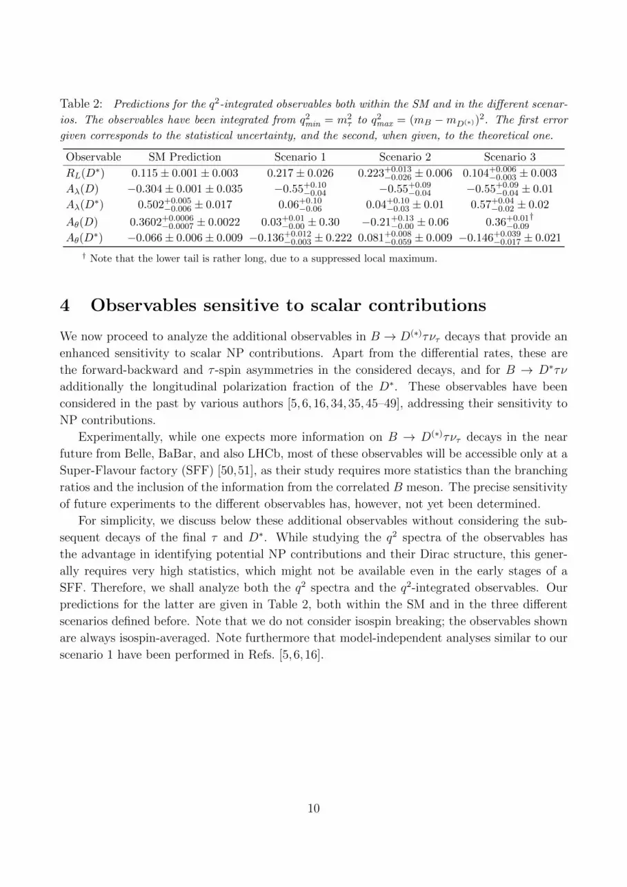
Table 2: Predictions for the q2-integrated observables both within the SM and in the different scenar-
ios. The observables have been integrated from q2min = m2
τ to q2max = (mB −mD(∗))2. The first error
given corresponds to the statistical uncertainty, and the second, when given, to the theoretical one.
Observable SM Prediction Scenario 1 Scenario 2 Scenario 3
RL(D∗) 0.115± 0.001± 0.003 0.217± 0.026 0.223+0.013−0.026 ± 0.006 0.104+0.006
−0.003 ± 0.003
Aλ(D) −0.304± 0.001± 0.035 −0.55+0.10−0.04 −0.55+0.09
−0.04 −0.55+0.09−0.04 ± 0.01
Aλ(D∗) 0.502+0.005−0.006 ± 0.017 0.06+0.10
−0.06 0.04+0.10−0.03 ± 0.01 0.57+0.04
−0.02 ± 0.02
Aθ(D) 0.3602+0.0006−0.0007 ± 0.0022 0.03+0.01
−0.00 ± 0.30 −0.21+0.13−0.00 ± 0.06 0.36+0.01
−0.09†
Aθ(D∗) −0.066± 0.006± 0.009 −0.136+0.012
−0.003 ± 0.222 0.081+0.008−0.059 ± 0.009 −0.146+0.039
−0.017 ± 0.021
† Note that the lower tail is rather long, due to a suppressed local maximum.
4 Observables sensitive to scalar contributions
We now proceed to analyze the additional observables in B → D(∗)τντ decays that provide an
enhanced sensitivity to scalar NP contributions. Apart from the differential rates, these are
the forward-backward and τ -spin asymmetries in the considered decays, and for B → D∗τν
additionally the longitudinal polarization fraction of the D∗. These observables have been
considered in the past by various authors [5, 6, 16, 34, 35, 45–49], addressing their sensitivity to
NP contributions.
Experimentally, while one expects more information on B → D(∗)τντ decays in the near
future from Belle, BaBar, and also LHCb, most of these observables will be accessible only at a
Super-Flavour factory (SFF) [50,51], as their study requires more statistics than the branching
ratios and the inclusion of the information from the correlated B meson. The precise sensitivity
of future experiments to the different observables has, however, not yet been determined.
For simplicity, we discuss below these additional observables without considering the sub-
sequent decays of the final τ and D∗. While studying the q2 spectra of the observables has
the advantage in identifying potential NP contributions and their Dirac structure, this gener-
ally requires very high statistics, which might not be available even in the early stages of a
SFF. Therefore, we shall analyze both the q2 spectra and the q2-integrated observables. Our
predictions for the latter are given in Table 2, both within the SM and in the three different
scenarios defined before. Note that we do not consider isospin breaking; the observables shown
are always isospin-averaged. Note furthermore that model-independent analyses similar to our
scenario 1 have been performed in Refs. [5, 6, 16].
10

4.1 The differential decay rates
First, we obtain the singly differential rates by summing in Eqs. (36) and (43) over the τ
helicities, λτ = ±1/2, and performing the integration over cos θ:
dΓ(B → Dτ−ντ )
dq2=G2F |Vcb|2|~p|q2
96π3m2B
(1− m2
τ
q2
)2 [|H0|2
(1 +
m2τ
2q2
)+
3m2τ
2q2|Ht|2
], (13)
dΓ(B → D∗τ−ντ )
dq2=G2F |Vcb|2|~p|q2
96π3m2B
(1− m2
τ
q2
)2 [(|H++|2 + |H−−|2 + |H00|2
) (1 +
m2τ
2q2
)+
3m2τ
2q2|H0t|2
]. (14)
Again, normalizing to the decays with light leptons reduces the theoretical error:
RD(∗)(q2) =dΓ(B → D(∗)τ−ντ )/dq
2
dΓ(B → D(∗)`−ν`)/dq2. (15)
Note that in order to obtain the expression for RD(∗) from this, numerator and denominator
have to be integrated separately. This should be kept in mind as well for the other quantities.
B®DΤΝΤ
4 6 8 100.00
0.05
0.10
0.15
0.20
0.25
0.30
0.35
q2@GeV2D
dBr�d
q2 @10
-2 G
eV-
2 D
B®DΤΝΤ
4 6 8 100
1
2
3
4
q2@GeV2D
RD
Hq2 L
B®D*ΤΝΤ
4 5 6 7 8 9 100.0
0.1
0.2
0.3
0.4
0.5
0.6
q2@GeV2D
dBr�d
q2 @10
-2 G
eV-
2 D
B®D*ΤΝΤ
4 5 6 7 8 9 100.0
0.2
0.4
0.6
0.8
1.0
q2@GeV2D
RD
*Hq2 L
Figure 3: The q2 dependence of the differential branching ratios (left) and RD(∗)(q2) (right), both
within the SM (grey) as well as in scenario 1 (red), scenario 2 (orange), and scenario 3 (yellow). The
binned distribution for RD(q2) is also shown.
Our predictions for these observables, within the SM and in the three different scenarios,
are shown in Fig. 3. For RD(q2), we show in addition the binned distribution in five equidistant
11

q2 bins, as the ratio does diverge at the endpoint, where however both rates vanish. From these
plots, we make the following observations:
• As expected, the uncertainty due to the hadronic form factors (the grey shaded band) in
RD(∗)(q2) is significantly reduced compared to that in the differential branching ratio.
• In scenario 2, relatively large deviations from the SM are predicted for almost the full
range in RD∗(q2) and for high q2 in RD(q2). The predicted q2 spectra in scenario 3 are
close to those of the SM, especially for the D∗ decay mode. However, there is still room
for differences, especially in RD(q2), and furthermore in this scenario the distribution in
RD∗(q2) lies preferably below the SM one, which should differentiate this scenario clearly
from the first two.
• Compared to the SM prediction, the peak of the differential branching ratio in the NP
scenarios (especially in scenario 2) is shifted to higher and lower values in q2 for the D and
the D∗ decay mode, respectively. This is characteristic of scalar NP contributions and
should allow for a separation from models with different Dirac structure. The reason for
that is the following: while both of them are explicitly proportional to q2 (see Eqs. (32)
and (39)), the charged-scalar contribution to RD∗(q2) is in addition proportional to the D∗
momentum |~p|, which vanishes at the endpoint q2max = (mB−mD∗)
2, rendering its relative
contribution maximal for intermediate values of q2, while the one to RD(q2) continuously
increases with q2. The relative suppression of the terms proportional to the τ mass by
the D∗ momentum furthermore renders RD∗(q2) finite everywhere, while RD(q2) diverges
at the endpoint.4 However, as both the rates for the τ and the light lepton modes
vanish there, this does not influence the experimental extraction: when calculating the
contributions to different bins, all integrals remain finite. These characteristic features
are illustrated by the right two plots.
As the charged scalar only contributes to the helicity amplitude H0t in B → D∗τντ decays,
an increased sensitivity is expected by studying the case with a longitudinally polarized D∗
meson in the final state, where the transverse helicity amplitudes are no longer relevant. For
this purpose, we define a singly differential longitudinal decay rate [5]:
dΓLτdq2
=G2F |Vcb||~p|q2
96π3m2B
(1− m2
τ
q2
)2 [|H00|2
(1 +
m2τ
2q2
)+
3m2τ
2q2|H0t|2
]. (16)
In analogy to RD∗(q2), it is again advantageous to consider the ratio with the τ mode normalized
to the light lepton mode:
R∗L(q2) =dΓLτ /dq
2
dΓL` /dq2. (17)
It is important, however, to note that within our NP framework this is not an independent
observable. As long as we consider only additional scalar operators, the difference
X1(q2) ≡ RD∗(q2)−R∗L(q2) (18)
4In fact, this behavior is an artifact of setting m` ≡ 0. The actual value is ∼ m2τ/m
2` .
12

is independent of NP effects. A measurement of this observable serves, therefore, as a cross-
check for the effect in RD∗ and gives us information on whether scalar NP operators are sufficient
to describe the data. This observation is reflected in Table 2 and in Fig. 4, where we show the
predictions for RL(D∗) and R∗L(q2) both within the SM and in the three different scenarios; the
results are analogous to the ones for R(D∗) and RD∗(q2) discussed above, but clearly exhibit
an increased sensitivity to the scalar NP effect.
B®D*ΤΝΤ
4 5 6 7 8 9 100.0
0.1
0.2
0.3
0.4
0.5
0.6
0.7
q2@GeV2D
RL* Hq2 L
Figure 4: Predictions for R∗L(q2) both within the SM and in the three different scenarios. The other
captions are the same as in Fig. 3.
4.2 The τ spin asymmetry
Information on the τ spin in semileptonic B-meson decays can be inferred from its distinctive
decay patterns [5, 16, 45, 49]. Therefore, we consider here the τ spin asymmetry defined in the
τ -ντ center-of-mass frame:
AD(∗)
λ (q2) =dΓD
(∗)[λτ = −1/2]/dq2 − dΓD
(∗)[λτ = +1/2]/dq2
dΓD(∗) [λτ = −1/2]/dq2 + dΓD(∗) [λτ = +1/2]/dq2, (19)
where the polarized differential decay rates are obtained after integration over cos θ of the
doubly-differential ones given by Eqs. (36) and (43). Using the formulae presented in appen-
dices C and D, we obtain explicitly
ADλ (q2) =|H0|2 (1− m2
τ
2q2)− 3m2
τ
2q2|Ht|2
|H0|2 (1 + m2τ
2q2) + 3m2
τ
2q2|Ht|2
,
AD∗
λ (q2) =(|H00|2 + |H++|2 + |H−−|2) (1− m2
τ
2q2)− 3m2
τ
2q2|H0t|2
(|H00|2 + |H++|2 + |H−−|2) (1 + m2τ
2q2) + 3m2
τ
2q2|H0t|2
. (20)
Again, these two observables have the same dependence on scalar NP contributions as the
differential rates; this observation follows from the combinations
XD2 (q2) ≡ RD(q2) (ADλ (q2) + 1) and XD∗
2 (q2) ≡ RD∗(q2) (AD
∗
λ (q2) + 1) (21)
13
being independent of δτcb and ∆τcb, respectively. However, because of the different normalization
and systematics in this case, a future measurement would give important information on the
size and nature of NP in B → D(∗)τν decays: like for X1(q2), any deviation from the SM value
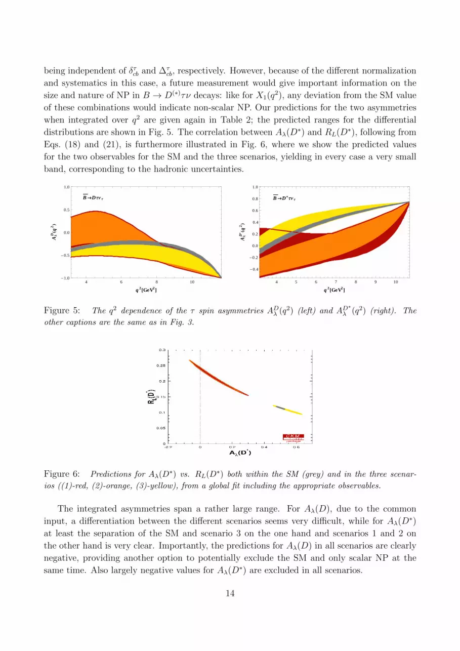
of these combinations would indicate non-scalar NP. Our predictions for the two asymmetries
when integrated over q2 are given again in Table 2; the predicted ranges for the differential
distributions are shown in Fig. 5. The correlation between Aλ(D∗) and RL(D∗), following from
Eqs. (18) and (21), is furthermore illustrated in Fig. 6, where we show the predicted values
for the two observables for the SM and the three scenarios, yielding in every case a very small
band, corresponding to the hadronic uncertainties.
B®DΤΝΤ
4 6 8 10-1.0
-0.5
0.0
0.5
1.0
q2@GeV2D
AΛD
Hq2 L
B®D*ΤΝΤ
4 5 6 7 8 9 10
-0.4
-0.2
0.0
0.2
0.4
0.6
0.8
1.0
q2@GeV2D
AΛD
*Hq2 L
Figure 5: The q2 dependence of the τ spin asymmetries ADλ (q2) (left) and AD∗
λ (q2) (right). The
other captions are the same as in Fig. 3.
Figure 6: Predictions for Aλ(D∗) vs. RL(D∗) both within the SM (grey) and in the three scenar-
ios ((1)-red, (2)-orange, (3)-yellow), from a global fit including the appropriate observables.
The integrated asymmetries span a rather large range. For Aλ(D), due to the common
input, a differentiation between the different scenarios seems very difficult, while for Aλ(D∗)
at least the separation of the SM and scenario 3 on the one hand and scenarios 1 and 2 on
the other hand is very clear. Importantly, the predictions for Aλ(D) in all scenarios are clearly
negative, providing another option to potentially exclude the SM and only scalar NP at the
same time. Also largely negative values for Aλ(D∗) are excluded in all scenarios.
14

The separation of the different models improves, once differential distributions are consid-
ered: from Fig. 5 we observe very distinct patterns for the different scenarios, especially for
scenario 2. This scenario will be clearly distinguishable from the SM and scenario 3, once the
necessary experimental precision is reached. Scenario 1, on the other hand, has again possibly
very large effects, but might be close to any of the other scenarios, including the SM. A char-
acteristic feature of this observable is the zero-crossing point: for ADλ (q2), it is absent for the
SM and scenario 3, while it appears likely for scenario 2 to have one, and also scenario 1 has
that option. Within the SM, the observable AD∗
λ (q2) crosses the zero at q2 = 3.66± 0.04 GeV2;
compared to the SM case, the zero-crossing point occurs at significantly higher values of q2 for
scenario 2, while most likely at lower values of q2 for scenario 3. This indicates that measuring
the zero-crossing point of the τ spin asymmetries can be a useful probe of the flavour structure
of the charged scalar interaction.
4.3 The forward-backward asymmetries
Finally, we discuss the forward-backward asymmetries defined as the relative difference between
the partial decay rates where the angle θ between the D(∗) and τ three-momenta in the τ -ντcenter-of-mass frame is greater or smaller than π/2:
AD(∗)
θ (q2) =
∫ 0
−1d cos θ (d2ΓD
(∗)τ /dq2d cos θ)−
∫ 1
0d cos θ (d2ΓD
(∗)τ /dq2d cos θ)
dΓD(∗)τ /dq2
. (22)
Using Eqs. (36) and (43), we arrive at the following explicit expressions:
ADθ (q2) =3m2
τ
2q2
Re(H0H∗t )
|H0|2 (1 + m2τ
2q2) + 3m2
τ
2q2|Ht|2
,
AD∗
θ (q2) =3
4
|H++|2 − |H−−|2 + 2m2τ
q2Re(H00H
∗0t)
(|H++|2 + |H−−|2 + |H00|2) (1 + m2τ
2q2) + 3m2
τ
2q2|H0t|2
. (23)
In terms of a model-independent determination of NP parameters, i.e. scenario 1, this is the key
observable to determine ∆τcb and δτcb. The reason, as mentioned before, is that the observables
R∗L(q2), RD(∗)(q2) and AD(∗)
λ (q2) do not give independent information, see Eqs. (18) and (21).
The forward-backward asymmetry AD(∗)
θ (q2) is therefore the only independent constraint in the
complex δτcb (∆τcb) plane. Our predictions for this observable are given in Table 2 and shown in
Fig. 7. Furthermore, its correlation with the τ spin asymmetry for the two modes is shown in
the first two panels in Fig. 8. It is clearly seen that the correlation is much weaker in this case,
especially in scenario 1, where the only influence stems from the restriction on |δτcb| and |∆τcb|.
However, the pattern of a more SM-like A2HDM prediction and strongly shifted predictions
from scenarios 1 and 2 is repeated. Regarding the differential distributions, within the SM,
the observable ADθ (q2) does not cross zero, while this becomes possible for scenarios 1 and 2.
AD∗
θ (q2) has a zero-crossing point at q2 = 5.67 ± 0.02 GeV2 in the SM, for which again large
shifts are possible with NP, and it might even vanish in scenario 3. Large deviations from the
SM expectations, especially in scenario 2, are therefore still possible for this observable.
15

B®DΤΝΤ
4 6 8 10-0.6
-0.4
-0.2
0.0
0.2
0.4
0.6
0.8
q2@GeV2D
AΘD
Hq2 L
B®D*ΤΝΤ
4 5 6 7 8 9 10-0.6
-0.4
-0.2
0.0
0.2
0.4
0.6
q2@GeV2D
AΘD
*Hq2 L
Figure 7: The q2 dependence of the forward-backward asymmetries ADθ (q2) (left) and AD∗
θ (q2) (right).
The other captions are the same as in Fig. 3.
In order to illustrate the impact of a possible future measurement of this observable, we
exemplarily show in the right panel in Fig. 8 the resulting constraint in the ∆τcb plane, together
with the one from R(D∗) as measured at the moment. The Aθ(D∗) constraints drawn in lighter
colours correspond to an uncertainty of 10%. For the darker constraints, an improvement
by a factor of 2 has been assumed compared to the lighter ones. Furthermore, an index
‘SM’ indicates the measurement chosen to be compatible with the SM, while the index ‘NP’
corresponds to measurements excluding the SM, but compatible with scenario 1. As can be
seen, such a measurement would allow to exclude a large part of the parameter space in the
model-independent scenario 1, as well as constrain the other scenarios further. Furthermore, as
mentioned before, the two constraints could also miss each other in that plane, indicating NP
with a different Dirac structure. This possibility exists of course also for the other observables
discussed above.
Additional information on ∆τcb could obviously be obtained from a measurement of the
B−c → τ−ντ rate. With the NP influence being determined by ∆τcb, this rate is clearly predicted
to be different from the SM in scenarios 1 and 2, while close to the SM in scenario 3. However,
this mode is extremely hard to be measured experimentally.
5 Summary
In this paper, motivated by the recent experimental evidence for an excess of τ -lepton produc-
tion in exclusive semileptonic B-meson decays, we have performed a detailed phenomenological
analysis of b → q τ−ντ (q = u, c) transitions within a framework with additional scalar opera-
tors, assumed to be generated by the exchange of a charged scalar in the context of 2HDMs.
While the usual Type-II scenario cannot accommodate the recent BaBar data on B →D(∗)τ−ντ decays, this is possible within more general models, in which the charged-scalar cou-
plings to up-type quarks are not as suppressed. An explicit example is given by the A2HDM, in
which the B → D(∗)τ−ντ as well as the B− → τ−ντ data can be fitted. However, the resulting
parameter ranges are in conflict with the constraints from leptonic charm decays, which could
16

Figure 8: Prediction for Aθ(D(∗)) vs. Aλ(D(∗)) for the SM (grey), and the three scenarios ((1)-red,
(2)-orange, (3)-yellow), from a global fit including all appropriate observables. The right plot shows
the possible impact of future measurements on the complex ∆τcb plane (see text).
indicate a departure from the family universality of the Yukawa couplings ςf (f = u, d, l).
These observations led us to define three scenarios for scalar NP, in which we incorporated
information from R(D(∗)) (Sc.1), B decays (Sc.2), and all available data from leptonic and
semileptonic decays apart from R(D∗) (Sc.3). We showed that these scenarios can be differ-
entiated by coming data, using information e.g. from differential decay rates and/or spin and
angular asymmetries. These observables therefore allow to verify this hint for NP in semilep-
tonic decays, and gather additional information on its precise nature. Furthermore we pointed
out several combinations of observables independent of this kind of NP, as well as common
characteristics, which will allow additionally to test for the presence of NP with other Dirac
structures. The coming experimental analyses for these modes will therefore be an important
step in our quest for NP.
Acknowledgements
A. P. would like to thank the Physics Department and the Institute for Advanced Study of
the Technical University of Munich for their hospitality during the initial stages of this work,
and the support of the Alexander von Humboldt Foundation. This work has been supported
in part by the Spanish Government [grants FPA2007-60323, FPA2011-23778 and CSD2007-
00042 (Consolider Project CPAN)]. X. Q. L. is also supported in part by the National Natural
Science Foundation of China (NSFC) under contract No. 11005032, the Specialized Research
Fund for the Doctoral Program of Higher Education of China (Grant No. 20104104120001) and
the Scientific Research Foundation for the Returned Overseas Chinese Scholars, State Education
Ministry. M. J. is supported by the Bundesministerium fur Bildung und Forschung (BMBF).
The work of A. C. is funded through an FPU grant (AP2010-0308, MINECO, Spain).
17

Table 3: Input values for the hadronic parameters, obtained as described in the text. The first error
denotes the statistical uncertainty, and the second the systematic/theoretical. †This value includes the
correction to the isospin limit usually assumed in lattice calculations [56, 69].
Parameter Value Comment
fBs (0.228± 0.001± 0.006) GeV [57–59]
fBs/fBd 1.198± 0.009± 0.025 [57,58,60]
fDs (0.249± 0.001± 0.004) GeV [57,58,60,61]
fDs/fDd 1.169± 0.006± 0.02 [57,58,60–62]
fK/fπ 1.1908± 0.0016± 0.0104† [62–64]
δK`2/π`2em −0.0069± 0.0017 [65–69]
δτK2/τπ2em 0.0005± 0.0053 [70–72]
λ 0.2254± 0.0010 [73]
|Vub| (3.51± 0.11± 0.02)× 10−3 [55]
|Vcb| (40.9± 1.1)× 10−3 [55]
ρ21 1.186± 0.036± 0.041 [55]
G1(1)|Vcb| (42.64± 1.53)× 10−3 [55]
∆|B→Dlν 0.46± 0.02 [7, 17,31]
hA1(1)|Vcb| (35.90± 0.45)× 10−3 [55]
R1(1) 1.403± 0.033 [55]
R2(1) 0.854± 0.020 [55]
R3(1) 0.97± 0.10 [36]
ρ2 1.207± 0.026 [55]
Appendix
A Input parameters and statistical treatment
Bounds on the parameter space are obtained using the statistical treatment based on frequen-
tist statistics and Rfit for the theoretical uncertainties [52], which has been implemented in the
CKMfitter package [12]. To fix the values of the relevant CKM entries, we only use determi-
nations that are not sensitive to the scalar NP contributions [12,53–55]. Explicitly, we use the
Vud value extracted from super-allowed nuclear β decays and the CKM unitarity to determine
Vus ≡ λ. The values of |Vub| and |Vcb| are determined from exclusive and inclusive b→ u`ν` and
b→ c`ν` transitions, respectively. Relevant hadronic input parameters are collected in Table 3,
while quark and meson masses as well as any other relevant parameters that do not appear in
this table are taken from [11].
The plots for the differential observables are obtained using the allowed NP parameter
ranges from a different fit. As the latter already include uncertainties from the hadronic input
parameters, we do not vary them again additionally.
18

B Kinematics for semileptonic decays
Within the SM, the squared matrix element for the decay B(pB)→ D(∗)(pD(∗) , λD(∗))l(kl, λl)ν(kν)
can be written as [34,35]
|M(B → D(∗)lν)|2 = |〈D(∗)lν|Leff |B〉|2 = LµνHµν , (24)
where the leptonic (Lµν) and hadronic (Hµν) tensors are built from the respective tensor prod-
ucts of the lepton and hadron currents. Using the completeness relation for the virtual W ∗
polarization vectors εµ(±, 0, t), one can further express Eq. (24) as
|M(B → D(∗)lν)|2 =∑
m,m′,n,n′
L(m,n)H(m′, n′) gmm′gnn′ , (25)
where gmm′ = diag(+1,−1,−1,−1), L(m,n) = Lµν εµ(m)ε∗ν(n) and H(m,n) = Hµν ε∗µ(m)εν(n).
The two quantities L(m,n) and H(m,n) are Lorentz invariant and can, therefore, be evaluated
in different reference frames. For convenience, the hadronic part H(m,n) is usually evaluated
in the B-meson rest frame with the z axis along the D(∗) trajectory, and L(m,n) in the l-ν
center-of-mass frame (i.e. in the virtual W ∗ rest frame) [34,35].
In the B-meson rest frame with the z axis along the D(∗) trajectory, a suitable basis for the
virtual W ∗ polarization vectors εµ(±, 0, t) can be chosen as [34]
εµ(±) =1√2
(0,±1,−i, 0) , εµ(0) =1√q2
(|~p|, 0, 0,−q0) ,
εµ(t) =1√q2
(q0, 0, 0,−|~p|) , (26)
where q0 = (m2B − m2
D(∗) + q2)/2mB and |~p| = λ1/2(m2B,m
2D(∗) , q
2)/2mB are the energy and
momentum of the virtual W ∗, with q2 = (pB − pD(∗))2 being the momentum transfer squared,
bounded at m2l ≤ q2 ≤ (mB −mD(∗))2, and λ(a, b, c) = a2 + b2 + c2− 2(ab+ bc+ ca). Similarly,
a convenient basis for the D∗ polarization vectors is
εα(±) = ∓ 1√2
(0, 1,±i, 0) , εα(0) =1
mD∗(|~p|, 0, 0, ED∗) , (27)
where ED(∗) = (m2B +m2
D(∗) − q2)/2mB is the D(∗) energy in the B-meson rest frame.
In the l-ν center-of-mass frame, which can be obtained by a simple boost from the B-meson
rest frame, the lepton and antineutrino four-momenta are given, respectively, as
kl = (El, pl sin θ, 0, pl cos θ) , kν = (pl,−pl sin θ, 0,−pl cos θ) , (28)
where El = (q2 + m2l )/2
√q2, pl = (q2 −m2
l )/2√q2, and θ is the angle between the D(∗) and l
three-momenta in this frame. The virtual W ∗ polarization vectors εµ(±, 0, t) reduce to [34,35]
εµ(±) =1√2
(0,±1,−i, 0) , εµ(0) = (0, 0, 0,−1) ,
εµ(t) =1√q2qµ = (1, 0, 0, 0) . (29)
19

With the above specified kinematics, the explicit expression for LµνHµν in terms of the q2
dependent helicity amplitudes can be found in Refs. [5, 34]. Using the equations of motion,
the hadronic and leptonic amplitudes of the scalar and the pseudoscalar current can be related
to those of the vector and the axial-vector current, respectively. Therefore, the scalar NP
contributions can be considered together with the spin-zero component (λW ∗ = t) of the virtual
W ∗ exchange.
C Formulae for B → Dlν
In the presence of NP of the form (2), the non-zero hadronic matrix elements of the B → D
transition can be parametrized as
〈D(pD)|cγµb|B(pB)〉 = f+(q2)
[(pB + pD)µ − m2
B −m2D
q2qµ]
+ f0(q2)m2B −m2
D
q2qµ , (30)
〈D(pD)|c b|B(pB)〉 =qµ
mb −mc
〈D(pD)|cγµb|B(pB)〉 =m2B −m2
D
mb −mc
f0(q2) , (31)
where mq are the running quark masses and the two QCD form factors f+(q2) and f0(q2) encode
the strong-interaction dynamics. Contracting the above matrix elements with the virtual W ∗
polarization vectors (26) in the B-meson rest frame, we obtain the two non-vanishing helicity
amplitudes [5, 34]:
H0(q2) =2mB|~p|√
q2f+(q2) ,
Ht(q2) =
m2B −m2
D√q2
f0(q2)
[1 + δlcb
q2
(mB −mD)2
], (32)
where δlcb, defined by Eq. (6), accounts for the contribution from the charged scalar.
It is customary to relate the QCD form factors f+(q2) and f0(q2) to the quantities G1(w)
and ∆(w) in the HQET [36]
f+(q2) =G1(w)
RD
, f0(q2) = RD(1 + w)
2G1(w)
1 + r
1− r∆(w) , (33)
where RD(∗) = 2√mBmD(∗)/(mB +mD(∗)), r = mD(∗)/mB, and the new kinematical variable w
is defined as
w = vB · vD(∗) =m2B +m2
D(∗) − q2
2mBmD(∗), (34)
with vB and vD(∗) being the four-velocities of the B and D(∗) mesons, respectively. We approx-
imate the scalar density ∆(w) by a constant value ∆(w) = 0.46 ± 0.02 [7, 17, 31] and G(w) is
parametrized in terms of the normalization G1(1) and the slope ρ21 as [74]
G1(w) = G1(1)[1− 8ρ2
1 z(w) + (51ρ21 − 10) z(w)2 − (252ρ2
1 − 84) z(w)3], (35)
20

with z(w) = (√w + 1−
√2)/(√w + 1 +
√2).
Equipped with the above information, the double differential decay rates for B → Dlν, with
l in a given helicity state (λl = ±1/2), can be written as
d2ΓD[λl = −1/2]
dq2d cos θ=
G2F |Vcb|2q2
128π3m2B
(1− m2
l
q2
)2
|~p| |H0(q2)|2 sin2 θ ,
d2ΓD[λl = +1/2]
dq2d cos θ=
G2F |Vcb|2q2
128π3m2B
(1− m2
l
q2
)2
|~p| m2l
q2|H0(q2) cos θ −Ht(q
2)|2 , (36)
from which the total decay rate and the various q2-dependent observables can be obtained via
summation over λl and/or integration over cos θ. Owing to its lepton-mass suppression, the
λl = +1/2 helicity amplitude is only relevant for the τ decay mode.
D Formulae for B → D∗lν
For the B → D∗ transition, the hadronic matrix elements of the vector and axial-vector currents
are described by four QCD form factors V (q2) and A0,1,2(q2) via
〈D∗(pD∗ , ε∗)|cγµb|B(pB)〉 =2iV (q2)
mB +mD∗εµναβ ε
∗νpαBpβD∗ ,
〈D∗(pD∗ , ε∗)|cγµγ5b|B(pB)〉 = 2mD∗ A0(q2)ε∗ · qq2
qµ + (mB +mD∗)A1(q2)
(ε∗µ −
ε∗ · qq2
qµ
)− A2(q2)
ε∗ · qmB +mD∗
[(pB + pD∗)µ −
m2B −m2
D∗
q2qµ
], (37)
from which one can show that, using the equations of motion, the B → D∗ matrix element for
the scalar current vanishes while the pseudoscalar one reduces to
〈D∗(pD∗ , ε∗)|cγ5b|B(pB)〉 = − qµmb +mc
〈D∗(pD∗ , ε∗)|cγµγ5b|B(pB)〉
= − 2mD∗
mb +mc
A0(q2) ε∗ · q. (38)
Contracting the above matrix elements with the W ∗ and D∗ polarization vectors in Eqs. (26)
and (27), we obtain the four non-vanishing helicity amplitudes [5, 34]:
H±±(q2) = (mB +mD∗)A1(q2)∓ 2mB
mB +mD∗|~p|V (q2) ,
H00(q2) =1
2mD∗√q2
[(m2
B −m2D∗ − q2) (mB +mD∗)A1(q2)− 4m2
B|~p|2
mB +mD∗A2(q2)
],
H0t(q2) =
2mB|~p|√q2
A0(q2)
(1−∆l
cb
q2
m2B
), (39)
21

where ∆lcb, defined by Eq. (4), accounts for the contribution from the charged scalar.
In the heavy-quark limit for the b and c quarks, the four QCD form factors V (q2) and
A0,1,2(q2) are related to the universal HQET form factor hA1(w) via [74]
V (q2) =R1(w)
RD∗hA1(w) ,
A0(q2) =R0(w)
RD∗hA1(w) ,
A1(q2) = RD∗w + 1
2hA1(w) ,
A2(q2) =R2(w)
RD∗hA1(w) , (40)
where the w dependence of hA1(w) and the three ratios R0,1,2(w) reads [74]
hA1(w) = hA1(1) [1− 8ρ2z(w) + (53ρ2 − 15) z(w)2 − (231ρ2 − 91) z(w)3] ,
R0(w) = R0(1)− 0.11(w − 1) + 0.01(w − 1)2 ,
R1(w) = R1(1)− 0.12(w − 1) + 0.05(w − 1)2 ,
R2(w) = R2(1)− 0.11(w − 1)− 0.06(w − 1)2 . (41)
The free parameters ρ2, R1(1) and R2(1) are determined from the well-measured B → D∗`ν
decay distributions [55] (` = e, µ), whereas for the parameter R0(1), that appears only in
the helicity-suppressed amplitude H0t, we have to rely on the HQET prediction for the linear
combination [36],
R3(1) =R2(1)(1− r) + r [R0(1)(1 + r)− 2]
(1− r)2= 0.97± 0.10 , (42)
which includes the leading-order perturbative (in αs) and power (1/mb,c) corrections to the
heavy-quark limit, plus a conservative 10% uncertainty to account for higher-order contribu-
tions [5].
Finally, the double differential decay rates for B → D∗lν, with l in a given helicity state (λl =
±1/2), can be written as
d2ΓD∗[λl = −1/2]
dq2d cos θ=
G2F |Vcb|2|~p|q2
256π3m2B
(1− m2
l
q2
)2
×[(1− cos θ)2 |H++|2 + (1 + cos θ)2 |H−−|2 + 2 sin2 θ |H00|2
],
d2ΓD∗[λl = +1/2]
dq2d cos θ=
G2F |Vcb|2|~p|q2
256π3m2B
(1− m2
l
q2
)2m2l
q2
×[sin2 θ (|H++|2 + |H−−|2) + 2 |H0t −H00 cos θ|2
], (43)
which are the starting point for the total decay rate, as well as the additional observables
considered.
22

References
[1] J. P. Lees et al. [BaBar Collaboration], Phys. Rev. Lett. 109 (2012) 101802
[arXiv:1205.5442 [hep-ex]].
[2] I. Adachi et al. [Belle Collaboration], arXiv:0910.4301 [hep-ex].
[3] A. Bozek et al. [Belle Collaboration], Phys. Rev. D 82 (2010) 072005 [arXiv:1005.2302
[hep-ex]].
[4] S. Fajfer, J. F. Kamenik, I. Nisandzic and J. Zupan, Phys. Rev. Lett. 109 (2012) 161801
[arXiv:1206.1872 [hep-ph]].
[5] S. Fajfer, J. F. Kamenik and I. Nisandzic, Phys. Rev. D 85 (2012) 094025 [arXiv:1203.2654
[hep-ph]].
[6] Y. Sakaki and H. Tanaka, arXiv:1205.4908 [hep-ph].
[7] D. Becirevic, N. Kosnik and A. Tayduganov, Phys. Lett. B 716 (2012) 208
[arXiv:1206.4977 [hep-ph]].
[8] B. Aubert et al. [BABAR Collaboration], Phys. Rev. D 81 (2010) 051101 [arXiv:0912.2453
[hep-ex]].
[9] J. P. Lees et al. [BABAR Collaboration], arXiv:1207.0698 [hep-ex].
[10] K. Hara et al. [Belle Collaboration], Phys. Rev. D 82 (2010) 071101 [arXiv:1006.4201
[hep-ex]].
[11] J. Beringer et al. [Particle Data Group Collaboration], Phys. Rev. D 86 (2012) 010001.
[12] J. Charles et al. [CKMfitter Group Collaboration], Eur. Phys. J. C 41 (2005) 1 [hep-
ph/0406184], updated results and plots available at: http://ckmfitter.in2p3.fr.
[13] N. Cabibbo, Phys. Rev. Lett. 10 (1963) 531; M. Kobayashi, T. Maskawa, Prog. Theor.
Phys. 49 (1973) 652.
[14] I. Adachi et al. [Belle Collaboration], arXiv:1208.4678 [hep-ex].
[15] A. Crivellin, C. Greub and A. Kokulu, Phys. Rev. D 86 (2012) 054014 [arXiv:1206.2634
[hep-ph]].
[16] A. Datta, M. Duraisamy and D. Ghosh, Phys. Rev. D 86 (2012) 034027 [arXiv:1206.3760
[hep-ph]].
[17] J. A. Bailey, A. Bazavov, C. Bernard, C. M. Bouchard, C. DeTar, D. Du, A. X. El-Khadra
and J. Foley et al., Phys. Rev. Lett. 109 (2012) 071802 [arXiv:1206.4992 [hep-ph]].
23

[18] R. N. Faustov and V. O. Galkin, Mod. Phys. Lett. A27 (2012) 1250183 [arXiv:1207.5973
[hep-ph]].
[19] N. G. Deshpande and A. Menon, arXiv:1208.4134 [hep-ph].
[20] D. Choudhury, D. K. Ghosh and A. Kundu, arXiv:1210.5076 [hep-ph].
[21] For a review, see for example: G. C. Branco, P. M. Ferreira, L. Lavoura, M. N. Rebelo,
M. Sher, J. P. Silva, Phys. Rept. 516 (2012) 1 [arXiv:1106.0034 [hep-ph]]; J. F. Gunion,
H. E. Haber, G. L. Kane, S. Dawson, Front. Phys. 80 (2000) 1.
[22] A. Pich, P. Tuzon, Phys. Rev. D 80 (2009) 091702 [arXiv:0908.1554 [hep-ph]].
[23] X. -G. He and G. Valencia, arXiv:1211.0348 [hep-ph].
[24] A. Pich, Nucl. Phys. Proc. Suppl. 209 (2010) 182 [arXiv:1010.5217 [hep-ph]].
[25] M. Jung, A. Pich, P. Tuzon, JHEP 1011 (2010) 003 [arXiv:1006.0470 [hep-ph]].
[26] M. Jung, A. Pich, P. Tuzon, Phys. Rev. D 83 (2011) 074011 [arXiv:1011.5154 [hep-ph]].
[27] M. Jung, X. -Q. Li and A. Pich, JHEP 1210 (2012) 063 [arXiv:1208.1251 [hep-ph]].
[28] W. -S. Hou, Phys. Rev. D 48 (1993) 2342.
[29] J. F. Kamenik and F. Mescia, Phys. Rev. D 78 (2008) 014003 [arXiv:0802.3790 [hep-ph]].
[30] O. Deschamps, S. Descotes-Genon, S. Monteil, V. Niess, S. T’Jampens and V. Tisserand,
Phys. Rev. D 82 (2010) 073012 [arXiv:0907.5135 [hep-ph]].
[31] G. M. de Divitiis, R. Petronzio and N. Tantalo, JHEP 0710 (2007) 062 [arXiv:0707.0587
[hep-lat]].
[32] K. Azizi, Nucl. Phys. B 801 (2008) 70 [arXiv:0805.2802 [hep-ph]].
[33] S. Faller, A. Khodjamirian, C. Klein and T. Mannel, Eur. Phys. J. C 60 (2009) 603
[arXiv:0809.0222 [hep-ph]].
[34] J. G. Korner and G. A. Schuler, Z. Phys. C 46 (1990) 93, ibid. C 38 (1988) 511 [Erratum-
ibid. C 41 (1989) 690].
[35] K. Hagiwara, A. D. Martin and M. F. Wade, Phys. Lett. B 228 (1989) 144, Nucl. Phys.
B 327 (1989) 569.
[36] A. F. Falk and M. Neubert, Phys. Rev. D 47 (1993) 2965 [hep-ph/9209268], Phys. Rev.
D 47 (1993) 2982 [hep-ph/9209269], M. Neubert, Phys. Rev. D 46 (1992) 2212.
[37] T. Hermann, M. Misiak and M. Steinhauser, arXiv:1208.2788 [hep-ph].
24

[38] [LEP Higgs Working Group for Higgs boson searches and ALEPH and DELPHI and L3
and OPAL Collaborations], hep-ex/0107031.
[39] A. Abulencia et al. [CDF Collaboration], Phys. Rev. Lett. 96 (2006) 042003 [hep-
ex/0510065].
[40] V. M. Abazov et al. [D0 Collaboration], Phys. Lett. B 682 (2009) 278 [arXiv:0908.1811
[hep-ex]].
[41] G. Aad et al. [ATLAS Collaboration], JHEP 1206 (2012) 039 [arXiv:1204.2760 [hep-ex]].
[42] S. Chatrchyan et al. [CMS Collaboration], JHEP 1207 (2012) 143 [arXiv:1205.5736 [hep-
ex]].
[43] M. -Z. Wang [Belle Collaboration], “Charm Decays at Belle”, talk given at ICHEP 2012,
Melbourne, Australia, July 4-11th, 2012.
[44] G. Rong, arXiv:1209.0085 [hep-ex].
[45] M. Tanaka, Z. Phys. C 67 (1995) 321 [hep-ph/9411405].
[46] C. -H. Chen and C. -Q. Geng, Phys. Rev. D 71 (2005) 077501 [hep-ph/0503123].
[47] C. -H. Chen and C. -Q. Geng, JHEP 0610 (2006) 053 [hep-ph/0608166].
[48] U. Nierste, S. Trine and S. Westhoff, Phys. Rev. D 78 (2008) 015006 [arXiv:0801.4938
[hep-ph]].
[49] M. Tanaka and R. Watanabe, Phys. Rev. D 82 (2010) 034027 [arXiv:1005.4306 [hep-ph]].
[50] T. Aushev et al., arXiv:1002.5012 [hep-ex].
[51] B. O’Leary et al. [SuperB Collaboration], arXiv:1008.1541 [hep-ex].
[52] A. Hocker, H. Lacker, S. Laplace and F. Le Diberder, Eur. Phys. J. C 21 (2001) 225
[hep-ph/0104062].
[53] M. Bona et al. [UTfit Collaboration], JHEP 0507 (2005) 028 [hep-ph/0501199].
[54] M. Antonelli et al., Phys. Rept. 494 (2010) 197 [arXiv:0907.5386 [hep-ph]].
[55] Y. Amhis et al. [Heavy Flavor Averaging Group Collaboration], arXiv:1207.1158 [hep-ex],
and online update at http://www.slac.stanford.edu/xorg/hfag.
[56] V. Cirigliano and H. Neufeld, Phys. Lett. B 700 (2011) 7 [arXiv:1102.0563 [hep-ph]].
[57] A. Bazavov et al. [Fermilab Lattice and MILC Collaboration], Phys. Rev. D 85 (2012)
114506 [arXiv:1112.3051 [hep-lat]].
25

[58] H. Na, C. J. Monahan, C. T. H. Davies, R. Horgan, G. P. Lepage and J. Shigemitsu,
Phys. Rev. D86 (2012) 034506 [arXiv:1202.4914 [hep-lat]].
[59] C. McNeile, C. T. H. Davies, E. Follana, K. Hornbostel and G. P. Lepage, Phys. Rev. D
85 (2012) 031503 [arXiv:1110.4510 [hep-lat]].
[60] C. Albertus et al., Phys. Rev. D 82 (2010) 014505 [arXiv:1001.2023 [hep-lat]].
[61] C. T. H. Davies, C. McNeile, E. Follana, G. P. Lepage, H. Na and J. Shigemitsu, Phys.
Rev. D 82 (2010) 114504 [arXiv:1008.4018 [hep-lat]].
[62] E. Follana et al. [HPQCD and UKQCD Collaborations], Phys. Rev. Lett. 100 (2008)
062002 [arXiv:0706.1726 [hep-lat]].
[63] C. Bernard, C. E. DeTar, L. Levkova, S. Gottlieb, U. M. Heller, J. E. Hetrick, J. Osborn
and D. B. Renner et al., PoS LAT 2007 (2007) 090 [arXiv:0710.1118 [hep-lat]].
[64] S. Durr, Z. Fodor, C. Hoelbling, S. D. Katz, S. Krieg, T. Kurth, L. Lellouch and T. Lippert
et al., Phys. Rev. D 81 (2010) 054507 [arXiv:1001.4692 [hep-lat]].
[65] W. J. Marciano, Phys. Rev. Lett. 93 (2004) 231803 [hep-ph/0402299].
[66] V. Cirigliano and I. Rosell, JHEP 0710 (2007) 005 [arXiv:0707.4464 [hep-ph]].
[67] V. Cirigliano and I. Rosell, Phys. Rev. Lett. 99 (2007) 231801 [arXiv:0707.3439 [hep-ph]].
[68] M. Antonelli, V. Cirigliano, G. Isidori, F. Mescia, M. Moulson, H. Neufeld, E. Passemar
and M. Palutan et al., Eur. Phys. J. C 69 (2010) 399 [arXiv:1005.2323 [hep-ph]].
[69] V. Cirigliano, G. Ecker, H. Neufeld, A. Pich and J. Portoles, Rev. Mod. Phys. 84 (2012)
399 [arXiv:1107.6001 [hep-ph]].
[70] W. J. Marciano and A. Sirlin, Phys. Rev. Lett. 71 (1993) 3629.
[71] R. Decker and M. Finkemeier, Nucl. Phys. B 438 (1995) 17 [hep-ph/9403385].
[72] R. Decker and M. Finkemeier, Nucl. Phys. Proc. Suppl. 40 (1995) 453 [hep-ph/9411316].
[73] J. C. Hardy and I. S. Towner, Phys. Rev. C 79 (2009) 055502 [arXiv:0812.1202 [nucl-ex]].
[74] I. Caprini, L. Lellouch and M. Neubert, Nucl. Phys. B 530 (1998) 153 [hep-ph/9712417].
26


