Service Provision on a Railway Network: A Laboratory Experiment

NET Institute*

www.NETinst.org

Working Paper #12-14

September 2012

Service Provision on a Railway Network: A Laboratory Experiment

Aurora Garcia-Gallego

Universitat Jaume I

Nikolaos Georgantzis Universitat Jaume I

Universidad de Granada

Gerardo Sabater-Grande Universitat Jaume I

* The Networks, Electronic Commerce, and Telecommunications (“NET”) Institute, http://www.NETinst.org, is a non-profit institution devoted to research on network industries, electronic commerce, telecommunications, the Internet, “virtual networks” comprised of computers that share the same technical standard or operating system, and on network issues in general.

1

Service provision on a railway network:

A laboratory experiment1

Aurora García-Gallego [a]

�ikolaos Georgantzís [a], [b]

Gerardo Sabater-Grande [a]

[a] Laboratorio de Economía Experimental & Economics Dept. Universitat Jaume I,

Castellón, Spain

[b] Economics Dept. Universidad de Granada, Granada, Spain

Abstract

Inspired by the ongoing debate regarding the liberalization of the Spanish railway network, we

use real-world information on the features of passenger transportation demand and the existing

network infrastructure to build a complex experimental setting. We test the efficiency of

alternative service provision obligations imposed to railway companies. Our results show that

imposing a minimum service for less profitable connections not only improves consumer and

overall welfare but will not harm the companies, because it enhances connectivity and the

overall demand on the network. In the absence of such service provision restrictions, the

companies failing to recognize the profitability of creating a complete network leave some

connections unserved, thus reducing overall demand for passenger services.

Key words: Transportation economics; railway networks; experimental economics; minimum

service restrictions.

1 We are grateful to the NET Institute www.NETinst.org for financial support. The OPTIRED project

sponsored by the Spanish Ministry of Science and Innovation was the starting point of this effort. All

errors and opinions contained hereby are the authors’ responsibility alone.

2

1. Introduction

Transportation networks are built over spaces which are defined and limited by

geographical specificities and geopolitical boundaries. Therefore, such networks are

exogenously bound to be asymmetric, contrary to the existing theoretical and

experimental approaches to social networks defined over abstract and, thus, ideal

spaces. Inspired more by the need for solutions to a real-world problem, rather than by

the aforementioned criticism to the received literature on networks, we focus here on an

existing railway network. Specifically, we use real-world information on the features of

passenger transportation demand and the existing network infrastructure of the railway

network in Spain, to build a complex experimental setting in order to test the efficiency

of alternative service provision obligations imposed to the railway operators.

The objective of this experiment is to analyze the influence of minimum service

restrictions on the schedules and fees chosen by the network operators on a railway

network. We propose three experimental treatments: a baseline without restrictions, and

two treatments with alternative minimum requirements. These minimum requirements

are designed to maximize social welfare based on the solution2 of a theoretical model.

Moreover, we are interested in analyzing the influence of the learning process by

decision makers on the network in the presence of competition for train connections and

routes. We propose a simple experimental network although, at the same time, we

capture the intrinsic characteristics of the rail network in Spain. We focus on the issues

of complementarities between stations or nodes on the network and substitutabilities

between slots. We are also the first to pay special attention on demand and cost

asymmetries allowing for a considerable degree of complexity in the decision making

process.

A rapidly growing literature has addressed similar issues regarding distribution

networks adopting a large spectrum of methodologies. Experiments have also been used

to address similar questions, although ours is the first to deal with an asymmetric

railway network. For example, Grether, Isaac and Plott (1981, 1989) analyze time slot

allocation in US airports. McCabe, Rassenti and Smith (1994) study the assignment of

the natural gas distribution network. More recently, Murphy et al. (2000, 2006) and

García-Gallego et al. (2012) studied the management of water distribution networks,

while Smith, Wilson and Rassenti (2001, 2002, 2003) and Ramírez-Escobar et al.

(2011) focused on electricity markets.

Regarding the privatization of railway network, Brewer and Plott (1996) confirm that a

second price auction is an appropriate market clearing mechanism leading to an almost

100% efficiency. Later, Nilsson (1999) showed that a repeated Vickrey auction could

also be a satisfactory way of assigning property rights in the use of a railway network.

Issacson and Nilsson (2003) compared the two mechanisms, finding insignificant

differences between them. Nilsson (2002) offers a mathematical optimization alternative

taking into account the administrative requirements for the management under the

alternatives studied. Parallel to the experimental methodology, a number of researchers

have used simulations, like those by Parkes and Ungar (2001), proposing more adequate

auctions to be used in a liberalized railway market. In such an environment, the German

2 See appendix 2 for more details.

3

Ministry of Education and Research has financed a study on auction mechanisms to be

used for an efficient assignment of time slots on the network. Borndorfer et al. (2005)

present a combinatorial auction as the solution to the problem in the German case under

study. The main problem solved there was related to possible cross-effects between a

local bottleneck and the remaining parts of the network, including low demand parts of

it.

Regarding the desirable competition framework Dutch authorities funded a study by

Cox et al. (2002) whose results based the Transportation Minister’s recommendation to

the Parliament. The recommendation was to choose competition for the market rather

than in the market in order to achieve the provision of the highest service quality at the

lowest fare possible, subject to minimum service restrictions.

In a context of liberalization of a railway service, our aim is to analyze how the

assignment of the rights of use of the network might be affected by minimum service

requirements. In particular we analyze the effect of compulsory service minima on the

schedule of trains and the fares implemented by the service providers. These minima are

aimed at increasing social welfare and they are calculated using a theoretical model in

which the network is administered by a unique benevolent operator. Our experimental

sessions have produced unprecedented results on the management of freight railway

transportation. Our findings indicate that the imposition of a minimum service on less

profitable connections ends up yielding higher welfare and even higher profits to private

operators than a fully decentralized regime, because unprofitable connections increase

the density of the network, leading to unexpected efficiency gains.

2. Methodology – Hypotheses

In order to reach our goal, we perform a laboratory experiment using a stylized and

reduced scale environment similar to that of the Spanish railway network as a test bed

for designing socially desirable minima to be fulfilled by the service providers,

competing for the different routes in an auction. We use two different approaches to the

problem in hand: First, we program an optimization algorithm to calculate the ideal

solutions (route schedules and fares) for each of the following cases: (a) Social welfare

maximization, (b) Social welfare maximization subject to the restriction that the

providers make nonnegative profits, (c) Profit maximization for a unique service

provider for the whole network. Second, we design an incentive compatible experiment

to test the theoretical predictions obtained. The economic laboratory allows economists

and policymakers to test and refine the market rules without incurring in the risks and

expenses of a real world trial. This type of experiments can be used to study

institutional mechanisms such as deregulation, privatization and public good provision.

These mechanisms are normally so complex that existing economic theory does not

offer precise predictions. In this way the lab constitutes a test bank where to examine

the behaviour of new proposed institutions, and, depending on the results, to modify its

rules and its implementation. This methodology can offer answers for questions such as

the assignment of air travel slots, communications license auctions, regulation in

markets, etc.

We analyze the effects of the imposition of welfare maximizing minima on: a) the

schedule of trains chosen by the operators, b) the fares charged in the auction process, c)

4

consumer surplus, d) supplier surplus, and e) social welfare. We are interested in

knowing if a regulator can be beneficial not only for the passengers but also for the

services providers, as far as it can overcome a myopic vision of the different rights of

use and take into account all the potential of a full-blown railway network.

We split our analysis into two big sections: the one referring to the strategic variables of

the model (fares and routes implemented by the service providers) and the one

concerning the outcome variables (competition structure emerging from the auctioning

of rights, final demand, network connectivity, providers’ profit, consumers’ surplus and

social welfare). We analyze the decision variables of the experiment participants: the

fares with which the would-be service providers bid for the franchises into which the

network is divided, and the routes that they offer once the franchises have been assigned

after the auction.

We address the following policy-relevant questions:

Question 1: Does learning in the management of the network affect the

fierceness of competition in the auction?

Question 2: Do service providers internalize the cost of the minimum service

provision restrictions imposed to them, and in what way?

Question 3: Does an increased experience in the management of the network

affect route scheduling?

Question 4: Are minimum service provision restrictions effective in increasing

service on less profitable routes?

Question 5: Do minimum service provision restrictions affect market structure

(number of different operators on the network)?

Question 6: Does experience in the management of the network affect the

number of passengers transported subject to route profitability?

Question 7: Do minimum service provision restrictions affect connectivity and

total demand?

Question 8: How does increased experience in network management affect

profits?

Question 9: How do minimum service provision restrictions affect consumer

surplus, profits and overall social welfare?

2.1 Supply and demand features

Providers face a mixed cost structure with fixed costs -reflecting the depreciation of the

trains- and variable costs linked to the service and including taxes for the use of the

infrastructure. For simplicity, we assume null additional marginal costs per passenger,

that is, there are no capacity restrictions. The cost structure is asymmetric and will

depend on the type of train used for a given route.

Our network is as simple as possible but at the same time, captures the main

characteristics of the Spanish railway network. The network is divided into regions,

stations and routes. We define a station as a place where passengers can embark and

disembark. A route is a link between stations and a region a set of stations where there

is a relevant concentration of passengers. The network runs on both directions, so it is

impossible to run more than one train in each direction at any time slot. Travelling from

5

one station to another inside a region requires one time slot. Travelling between

adjacent stations from different regions takes also one time slot.

We characterize the network defining as a product each combination formed by a route

and a time slot. There are complementarities between station pairs and substitutabilities

between time slots for that product. Complementarity between stations implies that the

demand for any route between two stations in a given time slot will be bigger if there

are connecting trains departing from the destination station or arriving to the departure

station in adjacent time slots. Substitutability between time slots implies that demand

for any route between two stations in a given time slot will be lower if there are other

trains in the same route in adjacent time slots. Also, we assume that demand is

negatively related with the transportation fare price and the travel time. Finally, demand

will be bigger in peak time slots than in valley time slots.

The network is represented in figure 1. It consists of five cities3, each constituting a

node. A combination of two nodes forms a route. In our network, there are two regions,

1-2-3 (Madrid-Cuenca-Albacete) and 1-4-5 (Madrid-Albacete-Alicante) and two links

2-4 (Cuenca-Albacete) and 3-5 (Valencia-Alicante). There is a two-way route between

any pair of adjacent stations. Besides these routes, in region 1-2-3, there is a direct two-

way route between Madrid and Valencia. This allows a fast train to travel from Madrid

(Valencia) to Valencia (Madrid), which would prevent running a train in the same time

slot going from Madrid (Valencia) to Cuenca or from Cuenca to Valencia. We call

connection to any combination of nodes that are not necessarily adjacent.

Figure 1: Railway network

The use of one train in different time slots is only restricted by purely physical

restrictions. In any station and time slot, a new train can be hired (assuming the

corresponding fixed and variable costs). A train which has been used in the preceding

time slot can be used again (assuming the corresponding variable costs) if it is available

in the station from where it should depart. As a simplifying assumption we consider

only 5 time slots, two of them (1 and 5) are considered peak slots and the rest (2, 3 y 4)

are considered valley slots due to their reduced passenger load.

3 In order to avoid geopolitical considerations by subjects, stations (cities) were codified with numbers in

the experimental sessions. Codes are 1=Madrid, 2=Cuenca, 3=Valencia, 4=Albacete and 5=Alicante.

6

The only strategic decision makers are the providers of railway transportation service.

The demand for the service is simulated by the computer program and is common

knowledge to the participants. In this way, demand Dtij for a route ij, where i, jϵ{1, 2, 3,

4, 5}, i≠j in a time slot t ϵ{1, 2, 3, 4, 5} is:

Dtij=DB

tij-P

tij-β(D

t-1ij+D

t+1ij)+δ(∑ki∈Cij D

t-1ki+ ∑jt∈Cij D

t+1jt) (1)

where Dtij is the basic demand corresponding to route ij at time slot t (different on each

route), Ptij is the fare charged for that particular route, C constitutes the set formed by all

routes in the same direction than ij arriving at i or departing from j. Last, βϵ(0,1) denotes

the substitutability degree between adjacent time slots (in our case it has been calibrated

to take a value of 0.2) and δ denotes the complementarity degree between stations (in

our case it takes a value of 0.3). In this way we observe that demand for a given route

will decrease with an increase in the fare for that route and with the existence of trains

in adjacent time slots for the same route. On the contrary, demand will increase if there

are connecting trains from other routes in adjacent time slots. In order to determine

consumer surplus in a given route at a given time slot, we simply subtract the fare paid

for the transportation from the reservation price determined by the demand function.

2.2 Experimental design

Each experimental session consists of 5 rounds, each of which with two parts: A and B.

In part A, the franchises are assigned for each route of the network, through an auction.

In the second part (B), the service providers decide which routes to schedule according

to the minimum requirements set up in the treatment (T0 is without minimum, T1 and

T2 have different minima) and the fare to which they committed in part A. The train

schedule planned by the subjects is carried out with the assistance of a software program

that avoids the collision of trains. In each round, there are four potential service

providers in the market, one for each available right to use or franchise in the network.

All potential service providers face the same entry conditions to the network. Franchises

are assigned through an auction in which providers bid proposing a fare for each route.

Subjects bid for the franchises in the two regions and for the two links described above.

Winners commit to run trains according to the licenses granted in part A of the round

but, occasionally (in treatments T1 and T2, not in T0), have to fulfil a minimum service

requirement in certain routes and time slots.

In part A of each round, the auction lasts at most five periods. In each auction period,

each potential provider can make at most four bids (one for each region/link), with a

maximum of twelve bids (three for each region/link) per provider in the five periods. At

the end of each auction period, the best bids are made public to all providers. The best

bid to obtain the franchise of a region or network link is the one that fixes the lowest

average fare for that segment. Each provider then knows, in each auction period,

whether he/she has the best bid for a certain zone so far. He/she is allowed to renew the

bid in the following period only if it is lower than the previous bid. The provider with

the best bid is considered so until the bid is improved upon in a subsequent period. In

that case, the new bid substitutes for the old one as the best bid. The winning bid is

determined in the last auction period, which is the fifth period with one exception:

7

starting in period 3, a new auction period does not start if none of the bids for the

network segments is improved upon. As a consequence, if there is no such improvement

in the period, this period is considered the last one and the one that determines the

winning bid.

Franchises are assigned through auction five times during the experiment (one for each

round). In this way, potential providers are allowed to learn, during the session, what

are the most advantageous fares to bid for each link, depending on their profits in

previous rounds.

In part B of each round, franchises are the ones that were assigned in part A. Part B

consists of five periods in which providers schedule their routes according to the

minimum requirements set in the treatment (no requirements in T0). In treatments T1

and T2, subjects are able to fix a service schedule that is above the minimum required,

but observing for all routes and time slots the fares they committed to in the auction

process (part A).

In each period, providers schedule their trains without knowing the decisions of the

other service providers in the network. Once all schedules have been set for the period,

the demand faced by each provider is simulated by the computer, following the structure

of the demand function presented earlier. This determines the provider’s revenues for

the period. The experiment is carried out under the condition of imperfect information.

Players do not know the functional form or the size of the market demand. The only

information available to subjects is the service schedule set by their rival providers, and

their fares. In the light of this information, providers can change their schedule in the

following periods. After these five scheduling periods, a new round starts in which

franchises are assigned again through a new auction.

Given the complexity of the experiment, it is necessary to instruct the participants prior

to the session in two aspects: (1) how to schedule trains in the experimental network and

how to fix fares taking into account the competition level and (2) how does the

franchise auction work. This longer than usual instruction phase, allows us to exclude

subjects failing to understand the aforementioned procedures. Nevertheless, instruction

is rewarded with a fixed amount of 10€ in order to compensate for the time the

participants dedicate. This amount is paid immediately after the session so that

participants get a fixed amount for the training and a variable amount of money for their

decisions in the experimental session.

The experiment consists of three treatments, with 80 participants4 each one and 25

decision rounds. In the baseline treatment (T0), there are no service minima that the

service providers have to take into account when competing for the rights of use of the

network. In the other two treatments (T1 and T2) we impose minimum levels of service

in the network aiming at maximizing social welfare. The minima are more demanding

in T2 than in T1. Two sessions of each treatment are programmed and run at the

Laboratorio de Economía Experimental (LEE) of the Universitat Jaume I in Castellón.

A total of 228 voluntary subjects were recruited among the Economics and Business

students using the ORSEE program, so that 57 markets with 4 subjects each (18, 20 and

4 8 participants in treatment 1 and 4 participants in treatment 3 were excluded after training period

because of their poor results, indicating lack of sufficient understanding of the task to perform.

8

19 markets for treatments T0, T1 and T2, respectively). This number of participants per

treatment allows us to have enough independent observations for the posterior statistical

analysis. Table 1 provides a summary of the main features of each treatment. Figures 2

to 5 are examples of screen-shots from the original5 (in Spanish) JAVA software used to

collect strategies and give feedback to the subjects from their past actions.6

Treatment Minimum

service

Rounds Sessions Subjects

T0 NO 25 2 72

T1 YES (M1) 25 2 80

T2 YES (M2) 25 2 76

TOTAL SUBJECTS 228 Table 1: Treatment details

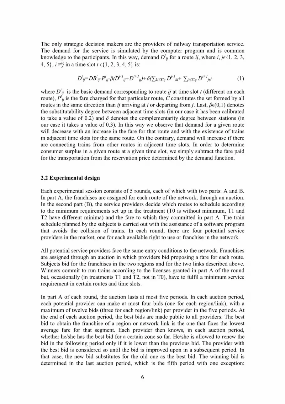
Figure 2: Decision screen for the auction

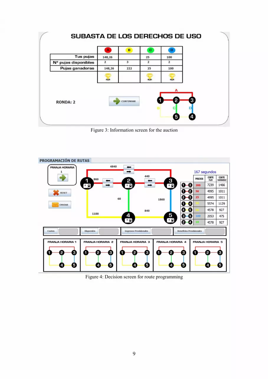
5 Glossary for Spanish-to-English translation of screen-shot text: “subasta de los derechos de

uso”=auction for the right to use; “puja disponible”=available bid; ronda=round; “confirmar

pujas”=confirm your bids; “tus pujas”=your bids; “pujas ganadoras”=winner bids; “programación de

rutas”=routes programming; “precios”=prices; “coste fijo”=fixed cost; “coste variable”=variable cost;

“segundos”=seconds; “franja horaria”=time slot; “ingresos”=income; “costes”=costs; “beneficio”=profits;

“period”=period; “demanda base”=basic demand; “continuar”=go. 6 The detailed instructions are available upon request from the authors.

9

Figure 3: Information screen for the auction

Figure 4: Decision screen for route programming

10

Figure 5: Information screen for route programming

Finally, the optimal routes and fees, calculated by the algorithm, as well as the resulting

restrictions imposed to the operators in the experiment are provided in appendix 2.

On the supply side, we assume that operators incur a fixed cost (FC) to rent a train and

cover the corresponding circulation costs and a variable cost (VC) associated with the

volume of passengers. In table 2 we present the cost values implemented in the

experiment:

Route 1-2 1-3 1-4 2-3 2-4 3-4 3-5

FC 4,995 7,239 5,574 4,995 4,578 2,053 4,578

VC 1,011 1,466 1,129 1,011 927 475 927

Table 2: Fixed and Variable Costs (FC, FC) per route used in the experiment

3. Results

3.1. Strategic Variables

In this section we report the results concerning the strategic variables: prices and routes.

3.1.1 Prices

In table 3 we present the winning price averages fixed per round on each connection

between network nodes.

11

T0 1-3 1-2 2-3 1-4 4-5 3-5 2-4

round 1 19.77 14.09 11.70 19.84 18.08 9.74 8.29

round 2 9.69 3.63 3.38 8.544 8.34 5.93 8.16

round 3 9.87 5.35 4.96 9.60 7.70 7.12 15.38

round 4 6.54 2.81 2.58 6.88 5.15 5.47 7.23

round 5 4.11 1.81 1.74 4.45 3.87 3.92 5.81

T1

round 1 15.03 18.72 18.65 16.86 16.18 8.55 9.08

round 2 9.23 13.73 14.88 10.69 10.10 7.53 9.58

round 3 7.84 12.32 11.689 8.30 7.66 6.50 8.47

round 4 6.27 10.16 11.331 8.80 7.72 3.96 11.09

round 5 6.17 8.29 7.786 8.11 6.37 6.17 8.79

T2

round 1 24.26 16.47 17.72 23.67 17.23 26.22 13.79

round 2 15.10 12.50 11.51 17.68 10.46 11.42 13.40

round 3 8.77 8.184 8.11 8.84 8.17 7.67 13.22

round 4 6.33 6.44 7.263 7.43 6.41 7.00 14.68

round 5 4.31 4.00 4.94 5.98 5.23 4.93 12.42 Table 3: Average prices generated in the auction process with franchise

We can observe that prices tend to decrease over time. Remember that during each

session, subjects participate in 5 auction periods assigning franchises. This process

captures possible inter-temporal patterns of behavior due to learning and other

dynamics. Figures 1-4 present average prices per round for each franchise zone: 1-2-3

(Madrid-Cuenca-Valencia), 1-4-5 (Madrid-Albacete-Alicante), 2-4 (Cuenca-Albacete)

and 3-5 (Valencia-Alicante). As we can observe, prices decline across rounds, except

for the case of the Cuenca-Albacete connection, which is also the least profitable. In

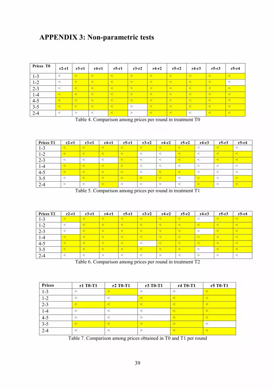
Appendix 3, tables 4-6 confirm that, overall, this pattern is statistically significant.

We, therefore, reach the following result:

Result 1: Learning dynamics during the network management process strengthen

competition, leading to a decline of prices across periods.

We now move to treatment effects on prices. We focus on price differences produced

depending on whether subjects were acting under a given minimum service restriction.

Figures 5-9 present price averages for the three treatments along the 5 rounds of each

session. A clear trend can be observed: on connections 1-2 (Madrid-Cuenca) and 2-3

(Cuenca-Valencia) differences among prices obtained in T0 and those in T1 or T2 are,

generally speaking, increasing over time. Thus, subjects seem to learn the profitability

of each market as the session advances. However, this is not possible in T1 and T2 in

which a service provision restriction exists.

Based on this observation and the statistical tests reported in tables 7-9 included in

Appendix 3 we state the following result:

Result 2: Operators reflect the extra cost imposed to them due to a service provision

restriction on higher prices when they are obliged to serve less profitable routes,

12

whereas the imposition of a minimum service on a profitable route does not affect

prices.

We move now to the frequency with which each possible market structure emerges in

our experiment. This information is reported on tables 10, 11 and 12. It can be observed

that monopoly and tetrapoly are the least frequent structures. Thus, intermediate degrees

of competition are achieved in most of the cases.

T0 Monopoly Duopoly Triopoly Tetrapoly

round 1 6% 56% 39% 0%

round 2 0% 44% 56% 0%

round 3 6% 33% 50% 11%

round 4 11% 39% 44% 6%

round 5 11% 44% 44% 0%

Table 10. Frequency for which each market structure may emerge in T0, per round


round 1 11% 63% 26% 0%

round 2 0% 65% 35% 0%

round 3 16% 47% 32% 5%

round 4 0% 50% 45% 5%

round 5 15% 50% 35% 0%



round 1 11% 63% 16% 11%

round 2 6% 56% 39% 0%

round 3 0% 42% 58% 0%

round 4 11% 42% 47% 0%

round 5 5% 63% 32% 0%


Figures 10, 11 and 12 present this information for treatments T0, T1 and T2,

respectively. We summarize our findings in the following result.

Result 3a: The learning process does not affect the resulting market structure.

Result 3b: Minimum service provision restrictions do not affect the resulting market

structure.

Looking at the prices contingent on the structure of the market, tables 13, 14 and 15

indicate that the expected pattern of lower prices in more competitive markets is not

confirmed.

13

Monopoly 1-3 1-2 2-2 1-4 4-5 3-5 2-4 T0 round 1 40 10 10 19 18 13.2 13.5 round 2 round 3 12 11 10 12 11 9 8.37 round 4 3 1.85 1.75 2 1.9 2.35 1.45 round 5 7.5 5 5 8 5 6.5 8 T1 round 1 21.67 20.67 19.67 23.67 13.33 10.33 5.83 round 2 round 3 2.83 5.2 6.67 3.79 3.32 2.03 5.77 round 4 round 5 3.99 8.5 4.23 6.5 2.17 2.21 7.63 T2 round 1 12.13 12.08 9.75 9.9 8.8 8.7 7.85 round 2 18 16 15 14 15 21 14 round 3 round 4 7 9.5 12.5 7.38 6.1 6.25 5.5 round 5 3.5 2 2 4 3 2.5 12

Table 13. Average prices from the auction for the monopoly

Duopoly 1-3 1-2 2-2 1-4 4-5 3-5 2-4 T0 round 1 11.25 9.72 7.13 24.62 21.75 9.53 8.09 round 2 10.94 4.25 3.75 7.5 8 5.71 7.94 round 3 13.73 8.5 7.5 7.83 6.28 6.91 8.67 round 4 7.34 8.29 4.29 7.64 6.41 5.75 6.86 round 5 3.24 1.21 1.18 3.39 2.78 3.11 3.94 T1 round 1 14.18 19.99 19.83 16.99 17.08 9.33 10.08 round 2 14.3 16.38 9 13.85 12.39 10.48 9.64 round 3 9.61 18.64 14.06 9.84 9.93 10.21 10.74 round 4 9.75 8 7 9.5 8.75 4.88 5.75 round 5 3.97 7.86 9.48 5.58 5.51 3.92 10.8 T2 round 1 10.96 9.47 6.98 23.65 21.04 10.94 7.35 round 2 8.69 2 1.25 6.5 6.94 5.08 7.94 round 3 16.12 8.33 6.67 5 4.07 3.83 7.16 round 4 7.9 5 5 8.15 7.48 6.20 7.46 round 5 3.10 1.30 1.27 3.79 3.36 3.09 3.5

Table14. Average prices from the auction for the duopoly

14

Triopoly 1-3 1-2 2-2 1-4 4-5 3-5 2-4 T0 round 1 29.07 20.93 18.50 13.14 12.86 9.56 7.86 round 2 8.36 2.86 2.82 8.98 7.93 5.83 7.86 round 3 7.81 3.68 3.68 12.98 9.48 7.41 25.06 round 4 7.06 2.13 1.63 7.07 5.52 6.00 8.84 round 5 4.49 1.44 1.28 5.64 4.43 4.58 7.50 T1 round 1 22.01 23.46 24.59 21.27 19.59 11.48 10.81 round 2 7.71 9.75 14.29 12.08 11.46 6.08 11.53 round 3 6.00 6.02 5.53 6.68 6.59 3.51 8.15 round 4 8.21 12.83 14.88 12.11 10.54 5.83 12.33 round 5 5.92 7.64 6.21 8.14 7.71 6.71 8.86 T2 round 1 32.36 25.07 22.79 16.42 15.42 10.38 8.86 round 2 7.55 1.39 1.33 8.42 7.58 5.13 7.61 round 3 7.49 3.27 3.27 12.09 8.53 6.92 22.61 round 4 7.06 2.13 1.63 7.07 5.52 6.00 8.84 round 5 4.68 1.81 1.91 6.39 5.68 4.96 7.25

Table15. Average prices from the auction for the triopoly

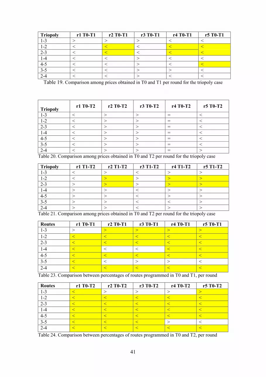
Figures 13-16 show price averages for each treatment by route. Regarding the

connection 1-2-3 (Madrid-Cuenca-Valencia), figure 13 indicates that prices tend to be

higher under service provision restrictions. Some time slots cannot be served by

operators acting under a restriction, which results in higher prices. Regarding

connection 1-4-5 (Madrid-Albacete-Alicante), figure 14 shows that the imposition of a

minimum service has no clear effect on prices as these routes are profitable. Regarding

connection 2-4 (Cuenca-Albacete), we can see on figure 15 that the imposition of

minimum services does not have a significant impact on prices. Finally, regarding the

connection 3-5 (Valencia-Alicante), no effect is observed according to figure 16. In

order to prove that this pattern is statistically significant, we include, in appendix 1,

tables 16 to 18 (corresponding to the duopoly case) and tables 19-21, that correspond to

the triopoly case.

We summarize the corresponding finding in the following result:

Result 4: Given a market structure, operators reflect on higher prices the extra cost

imposed to them by service provision restrictions obliging them to serve less profitable

routes.

3.1.2 Routes

In this subsection we present the empirical evidence obtained from the routes

programmed by operators through the franchise auction. For that purpose, we calculate

15

the percentage of routes programmed for each connection to the maximum of

potentially programmed routes. Table 22 shows the percentage of trains for each route.7

routes 1-3 1-2 2-3 1-4 4-5 3-5 2-4

T0

round 1 12.78 2.97 3.67 11.5 9.39 13.94 7.67

round 2 15.14 2.86 2.67 13.75 10.97 16.86 5.58

round 3 17.92 1.67 1.61 13.08 10.47 19.03 3.69

round 4 20.08 1.47 0.11 8.33 5.64 21.58 3.42

round 5 17.31 0.69 0.58 8.89 6.44 18.47 1.92

T1

round 1 11.1 9.83 8.5 18.93 19.25 16.5 10.15

round 2 10.13 8.63 7.45 14.78 14.98 17.73 6.1

round 3 11.33 8.83 7.25 16.73 16.08 17.88 7.98

round 4 10.7 9.65 8.47 17.73 17.28 19.15 9.45

round 5 11.88 8.98 7.6 16.98 17.18 20.25 6.03

T2

round 1 14.39 7.18 7 18.5 18.07 19.89 9.08

round 2 14.97 7.5 6.82 19.13 18.29 21.16 10.45

round 3 15 7.79 7.34 18.21 17.92 23.29 8.87

round 4 15 6.58 6.21 18.16 18.21 21.11 8.97

round 5 14.95 5.95 5.84 19.21 17.95 20.95 8.5

Table 22. Percentage of programmed routes per round and connection, by treatment

Figures 17 and 18 show that the percentages for connections 1-2 (Madrid-Cuenca) and

2-3 (Cuenca-Valencia) decrease to levels close to zero in treatment T0. This is due to

the fact that in T0 operators do not have a minimum to cover and, therefore, learning to

manage the network makes operators to abandon less profitable connections in favor of

the most profitable ones like 1-2 (i.e. Madrid-Valencia). This phenomenon is clear in

figure 19.

For the treatments in which a minimum is imposed, we can observe in figures 20 y 21,

the percentage of routes increases for connections in the area 1-4-5 (Madrid-Albacete-

Alicante).

Finally, figure 24 presents, for each treatment, the percentage of routes for average

round played. The differences between T0 and T1/T2 in connections 1-2 (Madrid-

Cuenca) and 2-3 (Cuenca-Valencia) are remarkable: low profitable routes that substitute

the high profitable route 1-3 (Madrid-Valencia). Moreover, although profitable, the

programming of the routes in the area 1-4-5 (Madrid-Albacete-Alicante) is positively

affected by the imposed minimum. We can find corresponding non parametric tests in

tables 23-25 included in the appendix.

The above analysis can be summarized in the following results:

7 A maximum of 2 trains can be programmed for each time table per connection. Therefore, the maximum

number of trains that can be programmed for each period for a given connection is 10, which implies that,

for each round (5 periods) this maximum is 50. The total trains’ number per connection divided by 50 and

multiplied by 100 gives us the percentage of trains per route.

16

Result 5a: Experience in the management of the network does not affect the

programming of profitable routes. The contrary is found for non profitable routes.

Result 5b: The imposition of service provision minima is particularly effective in

significantly increasing the routes programmed for less profitable connections.

However, such an imposition does not imply a significant increase in the use of more

profitable routes.

3.2 Outcome variables

In this section we analyze the following outcome variables: (a) final demand

(represented by travelers for each route), (b) connectivity generated in the network as

basic component of the final demand, (c) consumer surplus, (d) benefits of train

operators and (e) social welfare.

3.2.1 Final demand

First, in table 26 we present final demand of travelers for each connection per round

depending on implemented treatment.

1-3 1-2 2-3 1-4 4-5 3l-5 2-4

T0

round 1 1427717.27 64243.42 47727.73 319854.64 132022.49 589373.06 23879.73

round 2 1666730.80 65279.32 65583.21 330528.90 137335.34 667123.60 19370.37

round 3 1834887.11 22359.7 20657.75 275768.85 169453.42 670738.84 13757.55

round 4 2050802.32 3497.4 2198.4 218548.39 94860.24 786997.02 8426.15

round 5 1818687.26 13500 11220.73 232311.44 129198.78 693425.99 7559.46

T1

round 1 1786589.43 156932.36 166003 552123.22 361309.25 416515.02 179556.81

round 2 1733088.45 160142.10 169403.26 477962.89 207193.58 845232.72 46605.47

round 3 1860531.47 147118.53 145938.14 510224.99 195580.90 485208.16 182931.77

round 4 1853899.66 168656.16 186423.19 535519.85 368290.33 538466.67 176780.32

round 5 1894329.87 147122.40 162624.97 517587.07 372903.16 454202.63 524995.02

T2

round 1 2043746.79 115441.90 158569.15 510357.80 306154.36 872297.47 60580.37

round 2 2124011.84 113553.73 163997.58 515273.98 427219.96 778821.45 69454.90

round 3 2139992.10 118788.65 175600.41 516733.67 311292.11 960455.74 62003.80

round 4 2136291.13 107219.30 158909.77 514249.79 404250.61 883619.77 62668.95

round 5 2155033.34 103369.60 158131.79 531422.80 302998.24 908277.99 58957.79

Table 26. Average final demand per route and round for each treatment.

Figures 25 to 31 in the appendix show the evolution of average final demand for each

connection and per round. In particular, figures 25, 26 y 27 show average final demand

of travelers for connections among nodes 1-2-3 (Madrid-Cuenca-Valencia). In these

figures we can observe how in T0 the average number of passengers on less profitable

routes (1-2 and 2-3) collapses in favor of the more profitable route (1-3). On the

contrary, when a minimum schedule is imposed (this happens in T1 and T2), less

profitable routes show a stable pattern throughout the session because of the existing

commitment.

As for the region 1-4-5 (Madrid-Albacete-Alicante), unlike the previous case, figures 28

and 29 show a stable final demand in T0 highlighting the profitability perceived by

operators. On the other hand, the imposition of a minimum schedule causes an increase

in the number of passengers.

17

In figure 30 we can observe how a minimum schedule affects to a connection with

marginal profitability as 2-4 (Cuenca-Albacete), increasing the number of transported

travelers. The opposite is observed in figure 31, where the profitable connection 3-5

(Valencia-Alicante) is not affected by this imposition.

Finally, in figure 32 we show the positive effects of the imposed minimum on final

demand for the whole network.

Tables 27-29 included in Appendix 3 present non parametric tests corresponding to

average final demand comparisons among treatments per round.

Summarizing:

Result 6a: Given a profitable connection, experience in the management of the network

does not affect the number of travelers in that connection. However, for the less

profitable routes, having such experience enhances the difference between the average

number of travelers with and without minima.

Result 6b: The imposition of minimum service restrictions significantly increases the

number of travelers on less profitable routes. However, such an imposition does not

affect the rest of the routes.

3.2.2 Connectivity

In this section we address one of the critical components of final demand: the

connectivity generated in the network. Connectivity is not fully known by train

operators at the moment of programming their trains unless an operator is a monopolist.

Otherwise, connectivity depends on previously unknown routes scheduled for

competing operators.

In table 30 below, we present the average number of travelers gained for each route

because of the connectivity generated.

Connectivity 1-3 1-2 2-3 1-4 4-5 3-5 2-4 T0

round 1 236,634.24 108,729.16 188,691.41 274,788.64 7,449,140.85 14,259,763.8 158,443.76

round 2 284,651.9 117,691.87 225,020.83 129,658.72 11,859,391.6 12,416,973.4 171,357.59

round 3 262,991.95 87,997.94 198,888.60 168,868.36 11,456,035.8 13,104,759.2 139,073.39

round 4 270,927.54 64,862.98 222,826.39 31,429.14 5,697,474.32 5,350,954.7 90,828.82

round 5 251,316.97 70,983.68 199,626.32 42,617.62 8,428,097.16 9,702,149.37 110,460.39

T1

round 1 254,034.59 256,050.75 214,535.25 6,122,566.19 19992637.9 33,685,260.7 355,088.05

round 2 346,712.96 199,382.05 297,601.68 2,035,133.93 11029265.8 2,005,1178.9 292,951.39

round 3 255,791.95 239,840.33 232,166.66 2,387,715.82 12826476.6 18,143,983.2 287,337.09

round 4 280,180.45 255,962.70 251,176.75 2,385,777.12 16235228.9 27,250,663.6 361,632.94

round 5 248,803.79 342,714.53 319,382.45 5,790,256.51 13,126,281.4 28,892,092 346,389.65

T2

round 1 370,829.83 209,275.51 296,848.17 589,459.34 1,8107,618.7 29,694,180 313,851.47

round 2 349,325.84 215,152.14 274,686.58 1,386,600.89 1,9343,686.9 32,942,676 350,004.74

round 3 395,807.71 216,555.08 323,037.55 1,364,303.5 18,292,836.8 31,009,103.3 323,203.11

round 4 372,024.01 211,235.07 298,668.34 1,489,980.09 15,999,924 32,417,572.7 341,807.41

round 5 387,453.22 214,765.78 303,153.83 902,334.66 19,402,170.1 30,817,188 315,226.7

Table 30. Connectivity obtained by route and round for each treatment.

18

As shown in figure 33, the connectivity generated in the network is higher when

operators are forced to provide a minimum service. Note that, although operators do not

know routes scheduled by competing operators when deciding, in the case of T1 and T2

they are aware of the corresponding imposed minimum. This minimum provides helpful

information to operators with less profitable connections in order to predict more

precisely their potential final demand. In that sense the imposed minimum provides a

critical mass of traffic empowering the connectivity of the network system increasing

their potential final demand.


average connectivity comparisons among treatments per round.

We, therefore, get the following result:

Result 7: The imposition of minima results in higher network connectivity which

implies higher total demand. In order to satisfy the increased demand, operators make

traffic more dense, which, at the same time, generates more connectivity and a higher

total demand.

3.2.3 Profits

In table 34 we present, for each treatment, the average profits that operators get per

round and per connection.

1-3 1-2 2-3 1-4 4-5 3-5 2-4

T0

round 1 18945153 856391.94 251120.38 3768265.55 1268209.59 5449915.06 -349830.28

round 2 29215776.2 1088835.06 1310107.59 6043839.41 2062546.36 9419704.56 -10240.28

round 3 32946885.4 572066.1 524535.43 5643324.73 3810094.48 8454422.1 -30036.27

round 4 8985560.42 -97367.2 -538.2 995482.88 700608.32 2542214.08 -142967.65

round 5 6099442.27 3435.4 7276.45 527452.78 215055.94 2226006.07 -75502.47

T1

round 1 25869103.3 3033906.91 3242120.13 8036469.66 5544830.68 2941183.29 886699.26

round 2 13577854.9 1549939.08 2719115.59 3988363.68 1867607.42 5722006.01 -45688.34

round 3 13653279.5 1193623.6 1214018.1 2826528.83 179674.85 1240880.39 1107843.82

round 4 10014719.7 1076463.85 1787815.26 2747328.18 -248326.63 887696.14 954990.65

round 5 9421202.38 860085.46 1100954.94 2798241.74 1239064.25 439618.94 2353839.26

T2

round 1 48433782.9 1546093.5 2498129.91 10508891.7 4259534.13 21923252.9 28856490.9

round 2 32819002.1 1937536.72 2843496.09 9089550.3 4532048.78 11101168.4 908113.49

round 3 16503351.5 705179.2 1195251.51 3125794.67 1546682.98 6573581.02 335207.37

round 4 11336501 423615.65 886997.65 2375520.17 1379710.69 5620470.07 329812.23

round 5 7007125.21 186683.79 542563.01 1672070.55 788310.64 3881419.88 355781.38

Table 34: Average profits obtained by route and round for each treatment.

Figure 34 shows average profits of operators per round for each treatment implemented.

We observe a sharp decline of average profits as the session advances caused by

decreasing prices generated in the auction. Counter-intuitively, we can see that the

imposition of a minimum does not diminish the operatorsʼ profits by imposing

schedules containing unprofitable routes. This is so, because the imposition increases

final demand by means of higher connectivity, overcompensating losses caused by

lower prices.

19


average profits comparisons among treatments per round.

The above analysis can be summarized in the following result:

Result 8a: The negative trend in prices due to higher experience in the management of

the network has a significant negative effect in operators’ profits.

Result 8b: Given that the final demand of the network increases with the imposition of

restrictions, the latter do not negatively affect operators’ profits. This effect

compensates the loss in demand generated by the imposition of low demand routes.

3.2.4 Consumer Surplus

In table 38 we show average consumers surplus enjoyed by travelers per connection

each round depending on the treatment implemented.

1-3 1-2 2-3 1-4 4-5 3-5 2-4

T0 round 1 2709626663 21815232.2 13833429.2 146568538 54928493.2 404642741 2445107.21 round 2 3118920358 20652377.8 20816560.5 134850805 54365935.2 467541879 1504224.18 round 3 3363860718 7263878.61 6028044.68 110795203 71290814 456897695 1102916.26 round 4 3686282904 1344762.38 709989.93 90472728.1 38590895.5 536496240 559538.623 round 5 3353704033 3957481.4 4286726.86 97390266.4 57657668.8 480963247 611453.047 T1 round 1 3927679753 34140836.8 43772549.2 241563805 144080774 287760717 109860090 round 2 3858272946 739592106 40231789.7 136580182 77259088.6 358796418 105818996 round 3 4139539819 33440459.4 38231434.7 222601482 81435768.2 338132392 116309961 round 4 4119392305 39803563.2 51995255.7 232094407 163323409 364386641 110095693 round 5 4171023922 1000338865 38204630.2 131448651 63116850.7 397746750 120935647 T2 round 1 4321030404 25073562.3 53268516.2 230196760 124548775 609889941 6709951.37 round 2 4507974954 22651109.8 56629265.5 217045620 246391577 513390524 7837317.52 round 3 4551458940 23866140.3 60475701.5 222642153 132464798 660921582 7244122.72 round 4 4550416288 23119292.4 57159422.9 221549369 177802253 614409915 7340860.01 round 5 4591590907 23607235.5 59284236.9 228289481 127552795 645251643 6851632.61

Table 38: Average consumer surplus obtained by route and round for each treatment

As we can see in table 38 the surplus obtained by passengers in every route is higher

when operators are forced to fulfill a minimum schedule than when they freely program

their routes. These differences are especially significant in the case of routes with low

demand. In other routes, travelers are also favored to enjoy a more dense and

interconnected network. In figure 35 we observe how average consumer surplus

increases for the entire network when we impose a minimum schedule.

Tables 39-41 included in the appendix present non parametric tests corresponding to

average consumer surplus comparisons among treatments per round.

Result 9: The minimum service provision restrictions increases traveler surplus,

particularly in less profitable routes. Travelers of high-demand routes are also favored

due to a network with higher density.

20

3.2.5 Social Welfare

Lastly we deal with social welfare of society as sum of consumer surplus and operators

profits. In table 42, we present levels of social welfare generated in each market per

round depending on the treatment implemented.

In this case, the theoretical model is parameterized weighting travelers’ surplus more

than firmsʼ profits. Therefore results obtained in the former section are generally

replicated in this one.

1-3 1-2 2-3 1-4 4-5 3-5 2-4

T0

round 1 2728571816 22671624.2 14084549.6 150336803 56196702.8 410092656 2095276.93

round 2 3134287793 21076767.6 21407739.7 137509243 55226470.1 472648754 1349052.4

round 3 3380832443 7411110.41 6160082.9 113383375 72718548.2 461158332 914553.483

round 4 3695268464 1247395.18 709451.73 91468211 39291503.8 539038454 416570.972

round 5 3359791748 3960916.8 4294003.31 97906429.1 57867162.8 483184503 535950.575

T1

round 1 3953548856 37174743.7 47014669.3 249600274 149625605 290701900 110746789

round 2 3871850801 741142045 42950905.3 140568546 79126696 364518424 105773308

round 3 4153193098 34634083 39445452.8 225428010 81615443 339373273 117417805

round 4 4129741273 41115590.1 54000436 235277529 164511933 365451512 111198076

round 5 4180445124 1001198951 39305585.2 134246893 64355915 398186369 123289486

T2

round 1 4369464187 26619655.8 55766646.1 240705652 128808309 631813194 35566442.3

round 2 4537782516 23800037 58313580.2 224947635 249663313 522133401 8081077.97

round 3 4567962291 24571319.5 61670953 225767948 134011481 667495163 7579330.08

round 4 4561752789 23542908.1 58046420.6 223924889 179181964 620030385 7670672.24

round 5 4598598033 23793919.3 59826799.9 229961552 128341106 649133063 7207413.99

Table 42: Average social welfare obtained by route and round for each treatment

Additionally, tables 43-45 in the appendix present non parametric tests corresponding to

average social welfare comparisons among treatments per round.

From this, we can infer the following result:

Result 10: The minimum service provision restrictions increase consumer surplus and

do not negatively affect private operators’ profits due to an increase in total demand

caused by higher levels of network connectivity. In consequence society increase their

welfare thanks to the minimum imposed.

4. Conclusions

We have analyzed experimentally the effect of minimum service provision restrictions

on the overall usage of the railway network and the resulting prices. Our main finding is

that although such restrictions shift operators along less profitable routes, not only

21

increase social welfare but, rather unexpectedly increase private profits, as they force

operators to form a denser network leading to a higher overall demand. Thus, our results

support a liberalization process under the auspices of a regulator guaranteeing the

coverage of less profitable connections. In fact, such a regulator, apart from a consumer-

friendly institution, should be seen as a profit-preserving device for the sector as a

whole.

Finally, our overall approach shows how the use of laboratory experiments can

complement usual approaches based on empirical data and optimization algorithms and

simulations to assist the policy maker in the regulation of complex network markets like

the one studied here.

REFERE�CES

Abbink, K., Irlenbusch, B., Pezanis-Christou, P., Rockenbach, B., Sadrieh, A. and R.

Selten (2005), An experimental test of design alternatives for the British 3G/UMTS

auction, European Economic Review 49, 503-530.

Banks, J., Olson, M., Porter, D., Rassenti, S. and V. Smith (2003), Theory, experiment

and the Federal Communications Commission Spectrum Auctions, Journal of Economic

Behavior and Organization 51, 303-350.

Binmore, K. and P. Klemperer (2002), The biggest auction ever: the sale of the British

3G Telecom licences, Economic Journal, Royal Economic Society 112, C74-C96.

Borndörfer, R., Grötschel, M., Lukac, S., Mitusch, K., Schlechte, T., Schultz, S. and A.

Tanner (2005), An auctioning approach to railway slot allocation, ZIB Technical Report

ZR-05-45.

Brewer, P.J. and C.R. Plott (1996), A binary ascending price (BICAP) mechanism for

the decentralized allocation of the right to use railroad tracks, International Journal of

Industrial Organization 14, 857-86.

Cox, J.C., Offerman, T., Olson, M.A. and A. Schram (2002), Competition for versus on

the rails: a laboratory experiment, International Economic Review 43, 709–736.

Friedman, D. and S. Sunder (1994), Experimental methods. A primer for economists,

Cambridge University Press.

García-Gallego, A., Georgantzís, N., Hernán-González, R. and P. Kujal (2012), How do

Markets Manage Water Resources? An Experiment, Environmental and Resource

Economics 53, 1-23.

Grether, D.M., Isaac, R.M. and C.R. Plott (1981), The allocation of landing rights by

unanimity among competitors, American Economic Review 71, 166-71.

22

Grether, D.M., Isaac, R.M. and C.R. Plott (1989), The allocation of scarce resources:

Experimental economics and the problem of allocating airport slots, Westview Press,

Boulder, CO.

McCabe, K.A., Rassenti, S. and V.L. Smith (1994), Designing a real time computer

assisted auction for natural gas networks, in W. Cooper and A. Whinston (eds.), New

Directions in Computational Economics, Kluwer Academic Publishers, 41-54.

Murphy, J.J., Dinar, A., Howitt, R.E, Mastrangelo, E., Rassenti, S. and V.L. Smith

(2006), Mechanisms for addressing third-party impacts resulting from voluntary water

transfers. In: J.A. List (Ed.), Using experimental methods in environmental and resource

economics. Edward Elgar Publishing Ltd., Northampton, MA, 91-112.

Murphy, J.J., Dinar, A., Howitt, R.E., Rassenti, S. and V.L. Smith (2000), The design of

'smart' water market institutions using laboratory experiments, Environmental and

Resource Economics 17, 375-394.

Nilsson, J.E. (1999), Allocation of track capacity: Experimental Evidence on the use of

priority auctioning in the railway industry, International Journal of Industrial

Organization 17, 1139-1162.

Nilsson, J.E. (2002), Towards a welfare enhancing process to manage railway

infrastructure access, Transportation Research, A, 36, 419-36.

Issacson and Nilsson, J.E. (2003), An experimental comparison of track allocation

mechanisms in the railway industry, Journal of Transport Economics and Policy 37,

353-382

Parkes, D.C. and L.H. Ungar (2001), An auction-based method for decentralized train

scheduling, in Proc. 5th International Conference on Autonomous Agents (AGENTS-

01), 43-50.

Plott, C. (1997), An experimental test of the California electricity market,

http://www.energyonline.com/wepex/reports/reports2.html.

Rassenti, S., Smith, V.L. and R.L. Bulfin (1982), A combinatorial auction mechanism

for airport time slot allocation, Journal of Economics 13, 402-417.

Rassenti, S., Smith, V.L. and B.J. Wilson (2001), Turning off the lights, Regulation 24,

70-76.

Rassenti, S., Smith, V.L. and B.J. Wilson (2002), Using experiments to inform the

privatization/deregulation movement in electricity, The Cato Journal 21, 515-544.

Rassenti, S., Smith, V.L. and B.J. Wilson (2003), Controlling market power and price

spikes in electricity networks: Demand-side bidding, Proceedings of the National

Academy of Sciences 100, 2998-3003.

23

APPE�DIX 1: Figures and Tables

Figure 1: Per round average price for connection 1-2-3 (Madrid-Cuenca-Valencia)

Figure 2: Per round average price for connection 1-4-5 (Madrid-Albacete-Alicante)

Figure 3: Per round average price for connection 2-4 (Cuenca-Albacete)

0

5

10

15

20

25

1 2 3 4 5

Pric

e

round

t0

t1

t2

0

5

10

15

20

25

1 2 3 4 5

Pric

e

round

t0

t1

t2

0

2

4

6

8

10

12

14

16

18

1 2 3 4 5

Pric

e

round

t0

t1

t2

24

Figure 4: Per round average price for connection 3-5 (Valencia-Alicante)

Figure 5: Comparison of prices among connections (1-3, 1-2, 2-3, 1-4, 4-5, 3-5, 2-4) in round 1,

by treatment


by treatment

0

5

10

15

20

25

30

1 2 3 4 5

Pric

e

round

t0

t1

t2

0

5

10

15

20

25

30

mad-val mad-cu cu-val mad-Ab Ab-Al Val-Al Cu-Ab

Pric

e

Connections

r1 t0

r1 t1

r1 t2

0

2

4

6

8

10

12

14

16

18

20


Pric

e

Connections

r2 t0

r2 t1

r2 t2

25


by treatment


by treatment


by treatment

0

5

10

15

20


Pric

e

Connections

r3 t0

r3 t1

r3 t2

0

2

4

6

8

10

12

14

16


Pric

e

Connections

r4 t0

r4 t1

r4 t2

0

2

4

6

8

10

12

14


Pric

e

Connections

r5 t0

r5 t1

r5 t2

26

Figure 10: Market structures generated in T0, per round (Blue: Monopoly; Red: Duopoly; Green: Triopoly; Purple: Tetrapoly)


t0 r1 t0 r2 t0 r3 t0 r4 t0 r5

t1 r1 t1 r2 t1 r3 t1 r4 t1 r5

27


.

t2 r1 t2 r2 t2 r3 t2 r4 t2 r5

28

Figure 13: Average prices for each market structure in connection 1-2-3, by treatment

Figure 14: Average prices for each market structure in connection 1-4-5, by treatment

Figure 15: Average prices for each market structure in connection 2-4, by treatment

0

2

4

6

8

10

12

14

t0 t1 t2

Pric

e

Treatment

monopoly

duopoly

triopoly

0

2

4

6

8

10

12

14

t0 t1 t2

Pric

e

Treatment

monopoly

duopoly

triopoly

0

2

4

6

8

10

12

t0 t1 t2

Pric

e

Treatment

monopoly

duopoly

triopoly

29

Figure 16: Average prices for connection 3-5, by treatment and market structure

Figure 17: Percentage of routes for connection 1-2, by treatment and round

0

1

2

3

4

5

6

7

8

9

10

t0 t1 t2

Pric

e

Treatment

monopoly

duopoly

triopoly

30




31


Figure 22. Percentage of routes for connection 2-4, by treatment and round


32

Figure 24: Percentage of routes for each connection (1-3, 1-2, 2-3, 1-4, 4-5, 3-5, 2-4) and

treatment

Figure 25: Average final demand for connection 1-3, by treatment and round


0

500000

1000000

1500000

2000000

2500000

r1 r2 r3 r4

De

ma

nd

round

t0

t1

t2

0

20000

40000

60000

80000

100000

120000

140000

160000

180000

r1 r2 r3 r4 r5

De

ma

nd

round

t0

t1

t2

33




0

50000

100000

150000

200000

r1 r2 r3 r4 r5

De

ma

nd

round

t0

t1

t2

0

100000

200000

300000

400000

500000

600000

r1 r2 r3 r4 r5

De

ma

nd

round

t0

t1

t2

34



Figure 32: Average final demand for the whole network, by treatment and round

0

100000

200000

300000

400000

500000

600000

r1 r2 r3 r4 r5

De

ma

nd

round

t0

t1

t2

0

200000

400000

600000

800000

1000000

1200000

r1 r2 r3 r4 r5

De

ma

nd

round

t0

t1

t2

0

100000

200000

300000

400000

500000

600000

700000

r1 r2 r3 r4 r5

De

ma

nd

round

t0

t1

t2

35

Figure 33: Average connectivity generated for each treatment, per round

Figure 34: Average profits of operators for each treatment, per round

Figure 35: Average consumer surplus, by treatment and round

0,0E+00

2,0E+06

4,0E+06

6,0E+06

8,0E+06

1,0E+07

1,2E+07

1,4E+07

1,6E+07

1,8E+07

r1 r2 r3 r4 r5

round

profit t0

profit t1

profit t2

0,0E+00

1,0E+08

2,0E+08

3,0E+08

4,0E+08

5,0E+08

6,0E+08

7,0E+08

8,0E+08

9,0E+08

r1 r2 r3 r4 r5

round

CS t0

CS t1

CS t2

36

APPE�DIX 2: Theoretical optima and the resulting minimum provision

restrictions implemented in the experiment

Using the parameters considered for the cost and demand functions, we use an

algorithm to obtain optimum theoretical solutions (prices and routes) for the following

cases: (a) Maximization of social welfare, (b) Maximization of social welfare restricted

to non-negative profits for operators, (c) Maximization of monopolist profits.

(a) Maximization of social welfare

Given the cost structure of the model, the theoretical solution implies null prices in this

case. This is so because once a route is scheduled, the marginal cost of including an

additional travel is null. Therefore, fixing null prices, it is profitable for operators to

increase the number of passengers to the limit. Graphically, we show below the optimal

routes for each time slot:

(b) Maximization of social welfare restricted to non-negative profits for operators

Right to use 1-2-3: Price13 = 3.23; Price12 = 0.580; Price23= 0.292

37

Right to use 1-4-5: Price14 = 0.737; Price45= 0.559

Right to use 2-4: Price24 = 0.033

Right to use 3-5: Price35 = 1.248

(c) Maximization of monopolist’ profits

Right to use 1-2-3: Price13 = 1,727

Right to use 1-4-5: Price14 = 407; Price45= 309

Right to use 2-4: Price24 = 18

Right to use 3-4: Price35 = 689

Note that the theoretical solution that maximizes the profits of a monopolist operator

involves running no trains between stations 1 (Madrid) and 2 (Cuenca) and between 2

and 3 (Valencia) and programming fast trains to run between 1 and 3 in all time slots.

However if our objective is to maximize social welfare, we should schedule routes to

and from station 2 at certain time slots. We use this economic argument to implement

two minima in the provision of the service. In the baseline T0 no restriction is imposed,

in T1 and T2 operators must meet different minimum requirements based on social

welfare maximization. Below, we display, for each treatment, the minimum routes

required in each time slot:

Treatment 1:

38

Treatment 2:

39

APPE�DIX 3: �on-parametric tests

Prices T0 r2-r1 r3-r1 r4-r1 r5-r1 r3-r2 r4-r2 r5-r2 r4-r3 r5-r3 r5-r4

1-3 < < < < > < < < < <

1-2 < < < < > < < < < <

2-3 < < < < > < < < < <

1-4 < < < < > < < < < <

4-5 < < < < < < < < < <

3-5 < < < < > < < < < <

2-4 < > < < > < < < < <

Table 4. Comparison among prices per round in treatment T0


1-3 < < < < < < < < < <

1-2 < < < < < < < < < <

2-3 < < < < < < < < < <

1-4 < < < < < < < > < <

4-5 < < < < < < < > < <

3-5 < < < < < < < < < >

2-4 > < > < < > < > > <



1-3 < < < < < < < < < <

1-2 < < < < < < < < < <

2-3 < < < < < < < < < <

1-4 < < < < < < < < < <

4-5 < < < < < < < < < <

3-5 < < < < < < < < < <

2-4 < < > < < > < > < <


Prices r1 T0-T1 r2 T0-T1 r3 T0-T1 r4 T0-T1 r5 T0-T1

1-3 > > > > <

1-2 < < < < <

2-3 < < < < <

1-4 > < < < <

4-5 > < > < <

3-5 > < > > <

2-4 < < > < <

Table 7. Comparison among prices obtained in T0 and T1 per round

40



Duopoly r1 T0-T1 r2 T0-T1 r3 T0-T1 r4 T0-T1 r5 T0-T1 1-3 < < > < < 1-2 < < < < < 2-3 < < < < < 1-4 > < < < < 4-5 > < < < < 3-5 > < < > < 2-4 < < < > <

Table 16. Comparison among prices obtained in T0 and T1 per round for the duopoly case

Duopoly r1 T0-T2 r2 T0-T2 r3 T0-T2 r4 T0-T2 r5 T0-T2 1-3 > > < < > 1-2 > > > < < 2-3 > > > < < 1-4 > > > < < 4-5 > > > < < 3-5 < > > < > 2-4 > > > > >


Duopoly r1 T1-T2 r2 T1-T2 r3 T1-T2 r4 T1-T2 r5 T1-T2 1-3 > > < > > 1-2 > > > > > 2-3 > > > > > 1-4 < > > > > 4-5 < > > > > 3-5 < > > < > 2-4 > > > < >



1-3 < < > > <

1-2 < < < < <

2-3 < < < < <

1-4 < < > > <

4-5 > < > < <

3-5 < < < < <

2-4 < < > < <


1-3 < < < < >

1-2 < > > > >

2-3 > > > > >

1-4 < < < < >

4-5 < < < > >

3-5 < < < < >

2-4 < < < < <

41

Triopoly r1 T0-T1 r2 T0-T1 r3 T0-T1 r4 T0-T1 r5 T0-T1 1-3 > > > < < 1-2 < < < < < 2-3 < < < < < 1-4 < < > < < 4-5 < < > < < 3-5 < < > > < 2-4 < < > < <

Table 19. Comparison among prices obtained in T0 and T1 per round for the triopoly case

Triopoly

r1 T0-T2 r2 T0-T2 r3 T0-T2 r4 T0-T2 r5 T0-T2

1-3 < > > = < 1-2 < > > = < 2-3 < > > = < 1-4 < > > = < 4-5 < > > = < 3-5 < > > = < 2-4 < > > = >


Triopoly r1 T1-T2 r2 T1-T2 r3 T1-T2 r4 T1-T2 r5 T1-T2 1-3 < > < > > 1-2 < > > > > 2-3 > > > > > 1-4 > > < > > 4-5 > > < > > 3-5 > > < < > 2-4 > > < > >


Routes r1 T0-T1 r2 T0-T1 r3 T0-T1 r4 T0-T1 r5 T0-T1 1-3 > > > > >

1-2 < < < < < 2-3 < < < < <

1-4 < < < < <

4-5 < < < < < 3-5 < < > > <

2-4 < < < < <

Table 23. Comparison between percentages of routes programmed in T0 and T1, per round

Routes r1 T0-T2 r2 T0-T2 r3 T0-T2 r4 T0-T2 r5 T0-T2 1-3 < > > > > 1-2 < < < < <

2-3 < < < < < 1-4 < < < < <

4-5 < < < < <

3-5 < < < > < 2-4 < < < < <


42

Routes r1 T1-T2 r2 T1-T2 r3 T1-T2 r4 T1-T2 r5 T1-T2

1-3 < < < < <

1-2 > > > > >

2-3 > > < > >

1-4 > < < < <

4-5 > < < < <

3-5 < < < < <

2-4 > < < > <


Demand r1 T0-T1 r2 T0-T1 r3 T0-T1 r4 T0-T1 r5 T0-T1 1-3 < < < > <

1-2 < < < < < 2-3 < < < < <

1-4 < < < < <

4-5 < < < < < 3-5 > < > > >

2-4 < < < < <

Table 27. Comparison between average final demand in T0 and T1, per round

Demand r1 T0-T2 r2 T0-T2 r3 T0-T2 r4 T0-T2 r5 T0-T2 1-3 < < < < < 1-2 < < < < <

2-3 < < < < < 1-4 < < < < < 4-5 < < < < <

3-5 < < < < < 2-4 < < < < <

Table 28. Comparison between average final demand in T0 and T2 per round

Demand r1 T1-T2 r2 T1-T2 r3 T1-T2 r4 T1-T2 r5 T1-T2

1-3 < < < < <

1-2 > > > > > 2-3 > > < > >

1-4 > < < > > 4-5 > < < < >

3-5 < > < < <

2-4 > < < > >

Table 29. Comparison between average final demand in T1 and T2 per round

Connectivity r1 T0-T1 r2 T0-T1 r3 T0-T1 r4 T0-T1 r5 T0-T1 1-3 < < > < >

1-2 < < < < < 2-3 < < < < <

1-4 < < < < <

4-5 < > < < < 3-5 < < < < <

2-4 < < < < <

Table 31: Comparison between connectivity obtained in T0 and T1, by round and route

43

Connectivity R1 T0-T2 R2 T0-T2 R3 T0-T2 R4 T0-T2 R5 T0-T2 1-3 < < < < < 1-2 < < < < < 2-3 < < < < < 1-4 < < < < < 4-5 < < < < <

3-5 < < < < < 2-4 < < < < <


Connectivity r1 T1-T2 r2 T1-T2 r3 T1-T2 r4 T1-T2 r5 T1-T2

1-3 < < < < <

1-2 > < > > > 2-3 < > < < >

1-4 > > > > > 4-5 > < < > <

3-5 > < < < <

2-4 > < < > >


Profits r1 T0-T1 r2 T0-T1 r3 T0-T1 r4 T0-T1 r5 T0-T1 1-3 < > > < <

1-2 < < < < < 2-3 < < < < <

1-4 < > > < <

4-5 < > > > < 3-5 > > > > >

2-4 < > < < <

Table 35: Comparison between profits obtained in T0 and T1, by round and route

Profits r1 T0-T2 r2 T0-T2 r3 T0-T2 r4 T0-T2 r5 T0-T2 1-3 < < > < < 1-2 < < < < <

2-3 < < < < < 1-4 < < > < <

4-5 < < > < <

3-5 < < > < < 2-4 < < < < <


Profits r1 T1-T2 r2 T1-T2 r3 T1-T2 r4 T1-T2 r5 T1-T2

1-3 < < < < >

1-2 > < > > >

2-3 > < > > >

1-4 < < < > >

4-5 > < > < >

3-5 < < < < <

2-4 < < < > >


44

Consumer

Surplus r1 T0-T1 r2 T0-T1 r3 T0-T1 r4 T0-T1 r5 T0-T1

1-3 < < < < < 1-2 < < < < < 2-3 < < < < < 1-4 < < < < < 4-5 < < < < < 3-5 > > > > > 2-4 < < < < < Table 39: Comparison between consumer surplus obtained in T0 and T1, by round and route

Consumer


1-3 < < < < <

1-2 < < < < <

2-3 < < < < <

1-4 < < < < <

4-5 < < < < <

3-5 < < < < <

2-4 < < < < <

Tabla 40: Comparison between consumer surplus obtained in T0 and T2, by round and route

Consumer


1-3 < < < < <

1-2 > > > > >

2-3 < < < < <

1-4 > < < > <

4-5 > < < < <

3-5 < < < < <

2-4 > > > > >

Table 41: Comparison between consumer surplus obtained in T1 and T2, by round and route

S. Welfare r1 T0-T1 r2 T0-T1 r3 T0-T1 r4 T0-T1 r5 T0-T1

1-3 < < < < <

1-2 < < < < <

2-3 < < < < <

1-4 < < < < <

4-5 < < < < <

3-5 > > > > >

2-4 < < < < <

Table 43: Comparison between social welfare obtained in T0 and T1, by round and route

45


1-3 < < > < <

1-2 < < < < <

2-3 < < < < <

1-4 < < > < <

4-5 < < > < <

3-5 < < > < <

2-4 < < < < <



1-3 < < > < <

1-2 > > > > >

2-3 < < > < <

1-4 > < > > <

4-5 > < > < <

3-5 < < > < <

2-4 > > > > >


Documents

Service Provision on a Railway Network: A Laboratory Experiment