Sex and migration: who is the tied mover?

Draft, June 2006

Sex and Migration: Who is the Tied Mover?

By

Johanna Astrom♣

Olle Westerlund♣♣

Abstract We study the effects of interregional migration on two-earner households’ gross earnings and on the relative income between married/cohabiting men and women. In particular, we examine the nexus between education level and the relative income gains between spouses. The empirical analysis is based on longitudinal data from Sweden and functional regional labour markets as regional entities. Using difference-in-differences propensity score matching it is found that migration generally in-creases total gross wage earnings of households and has no significant impact on the male/female earnings gap. We find that the pre-migration level of education is a key determinant of migration and the economic outcome, and to some extent also for the effect on income distribution within the house-hold. The positive average effect on household earnings is largely explained by the income gains among highly educated males. Females experience on average no significant income gain in absolute terms from migration. However, the female educational level seems to be positively correlated with the effect on earnings, although the effect appears to be small. The relative male/female educational level seems to affect the relative income gain between spouses in the anticipated direction. However, significant increase in the female share of household income is indicated only for the sample of highly educated females married/cohabitant with males having a lower level of education.

♣ Department of Economics, Umeå University, SE-901 87 Umeå, Sweden. E-mail: [email protected] ♣♣ Department of Economics, Umeå University, SE-901 87 Umeå, Sweden. E-mail: [email protected].

mailto:[email protected]

mailto:[email protected]

Introduction

Investments in human capital, for example in health, education, and migration, are important

events for individuals, households, and on the aggregate also for the society. In a reasonably

functioning economy, these investments are expected to increase welfare and, under certain

circumstances, also the productivity of labour. Potentially, they may also have substantial

effects on the income distribution among income earners in general as well as within

households. Investments in education and geographical mobility may provide opportunities to

reduce the income differences between males and females, but may as well reinforce existing

income differences by asymmetrical favouring the careers of one of the sexes.

Empirical economic research on migration has typically been oriented towards the

determinants of migration and, to a somewhat lesser degree, towards the effects on income

among singles or couples. Only a small fraction of the research on migration has been

purposed for the study of the effects on intra-household income distribution. To the best of

our knowledge, there is no previous study that examines the determinants of changes in

family income distribution among households who relocates to another geographical labour

market.

Cooke (2003) studies married couples in the US and finds that migration increases in the

husband’s income and leaves the wife’s income unchanged, which is in line with the results in

an early study from the US by Sandell (1977). Cooke finds that this applies even in cases

where the wife has greater earning potential than her husband. Smits (2001) uses data on

married couples in the Netherlands and finds negative effects of migration on earnings for

both spouses. It is also found that most long-distance moves seem to be undertaken for the

career of the males. Jacobsen and Levin (2000) study interstate migration in the US during the

1980’s and report income gains only for the sample of single women. For married couples,

they find that the economic outcome of migration is negative and they find no effects of

migration on the relative income between spouses. Nivalainen (2002) studies Finnish

households and finds that migration for the most part occurs due to the demands of the

husband’s career, resulting in the wives being tied migrants. Employment after migration is

examined in Nivalainen (2004). The results show that employment among the majority of

2

men is unaffected. However, some groups of migrating husbands have higher employment

probability after migration, while the women never realize positive returns in terms of

employment. Using data on stable two-earner households in Sweden, Axelsson and

Westerlund (1998) find that migration does not affect real disposable income. Also based on

Swedish data, Nilsson (2000) concludes that migration increases the intra-household income

gap within young dual-university graduate households.

This study examines the effects of migration on the households total gross wage earnings and

the relative income between married/cohabitating males and females. We devote special

attention to the nexus between education and the relative outcome of migration for the

spouses. The reason for this is that the educational level of spouses is a potential indicator of

bargaining power which plays a decisive role in modern theories of intra household income

distribution (Lundberg and Pollak, 1996, 2001). The relevance of studies within this field of

research is also underlined by related international trends, such as the increased number of

two earners households, increasing investments in education, the increased share of females

entering higher education, and increasing interest in the issue of gender equality.

The empirical analysis is based on longitudinal data from Sweden. We use a large sample of

individuals who were married or cohabitants prior to and after migration. The sample is

confined to stable couples, both spouses being employed prior to migration. Sweden provides

an excellent ground for exploring these questions because of the availability of data, and

because of an internationally high labour force participation rate among women. The

remainder of this paper unfolds as follows. The next section gives a brief reference to theories

of distribution within the family and family migration. Section III presents the data and

estimation strategy. Section IV gives the estimation results. The final section contains

conclusions and discussion.

3

II Income distribution within the family and migration

One of the most common theoretical framework in economic studies of migration is the

standard human capital model where individual utility varies across potential locations and

the single individual chooses to reside in the location that maximizes utility, given location

specific benefits and costs (including eventual costs for relocation). For the single decision

maker, the model provides straightforward implications. For families, the decision to invest in

migration is much more complex.

Early models of family behaviour, labelled as common preferences models, the consensus

model (Samuelson, 1956) and the altruist model (Becker, 1974), imply that family decisions

are consistent with maximising a single utility function. A common feature of the common

preference models is pooling of incomes, meaning that incomes of e.g. a husband and wife are

pooled and the allocation of expenditures is independent of the relative contribution of

husband and wife. This means that a given increase in income has the same effect on utility

and consumer demand irrespective of which of the spouses that brings home the bacon.

Empirical evidence is, however, generally not consistent with the income pooling assumption

and more recent bargain models of family decisions seem to provide a more credible

description of the migration decision than the common preferences models does (see e.g.

Lundberg and Pollak, 1996).

The decision to invest in migration for a two-earner household has to satisfy both spouses and

the optimal location for the family may not be the optimal location for any of the two spouses

if being single. When a spouse moves along with her partner even though the individual gain

from “family optimum” is lower than the gain from a “free optimum”, it is commonly

throughout the literature called tied migration. At the optimal location for the family, the total

family utility is maximized and the tied migrant has to receive enough compensation from the

partner to migrate and stay in the relationship (Mincer, 1978). Analogously, one spouse may

also be a tied stayer, receiving enough compensation from the other spouse to stay at the

present location and stay in the marriage. It is, of course, also possible that both spouses are

tied migrants or tied stayers.

4

In a bargaining model the individuals are assumed to maximize their individual utility and the

behaviour of the family are not only dependent on total family income (ceteris paribus) but

also on the determinants of the payoff in case of no agreement, the threat point (Lundberg and

Pollak, 1996). The threat point can be either external, e.g. divorce, or internal an inefficient

non-cooperative equilibrium within marriage. The most extreme threat point is, for most

couples, likely to be divorce where the threat point and the bargained outcome depend on

environmental factors such as the spouse’s possibilities and opportunities outside the

marriage. In everyday bargaining the internal threat point is more plausible. In this case the

family’s demands depend on who receive income within the marriage. The bargained

outcome will depend upon the utility at the threat point and the decisions of the family will

depend on who receives the higher income within the marriage. It is however reasonable to

assume that the allocation problem has an external threat point, if the spouses can not agree on

a residential location they separate or divorce.

In the human capital model, where a single utility function is maximized, it is assumed that

the tied mover will be compensated for the loss it suffers from migration. The cooperative

bargaining models assume that all agreements can be reinforced and that there is no restriction

on the agreements made within the family. However it is not very likely that the couple can

make binding agreements about future distribution of resources within the marriage.

Lundberg and Pollak (2001) illustrate a non-cooperative two-stage game where the location is

determined in the first stage and the distribution of resources between spouses in the second.

Given that the investment in human capital yield different returns for the two individuals, the

bargaining power in future bargaining will be affected and thereby the spouses possibilities to

claim family resources in the future. If it is impossible for the spouses to make binding

agreements about future transfers of resources, the allocation problem may have an inefficient

outcome. The spouses realize that their bargaining power will be altered and this can lead to

either an inefficient location or inefficient divorce. An inefficient location is characterized by

not maximizing the total income for the household. The tied spouse prefers a bigger piece of a

smaller pie and the leader prefers being married to the alternative of receiving a higher

income and being separated.

Thus, modern theories seem to accommodate empirical observations that are inconsistent with

the older common preferences / income pooling models, and they generate several interesting

5

and seemingly realistic implications. It appears, however, as extremely difficult to pursue

rigorous empirical tests of these models and we make no such aspiration.1 In fact, previous

studies perform tests of older models based on unrealistic assumptions. Still, previous

empirical results are valuable and interesting in many respects. This study is also of

explorative nature and adds, in our view, substantial contributions in relation to previous

empirical research within this field. The specific empirical questions to be addressed are:

- does migration yield an income gain for the household as a whole?

- does migration affect the relative income between spouses?

- how are changes in relative earnings related to potential proxies for bargaining power,

such as level of education and previous income?

Educational level is a good proxy for potential wage level and it is therefore reasonable to

think that it would affect the family’s location decision, and consequently also the returns

from migration for the male and the female. Moreover, the bargaining models suggest that

some of the covariates in empirical household models of migration and post-migration

income, may be perceived as indicators of bargaining power. As pointed out by Lundberg and

Pollak (2001), education and pre-migration income are two possible candidates in this respect.

1 Naturally, changes in wages or incomes do not translate into changes in utility by necessity. It is, for example, extremely difficult to incorporate indicators of compensating wage and income differentials into empirical models.

6

III Data and estimation

We use annual panel data from various official registers by the Swedish National Tax Board,

the National Labour Market Administration of Sweden, and Statistics Sweden. The sample

pertains to residents in Sweden who were married or cohabitants in stable household

constellations between 1997 and 2003. We have included couples where both spouses were

employed in 1997 and where there exits observations on the earnings 1997-2003. The final

sample includes 125 891 couples out of which 1 911 have migrated in 1998 or 1999.

Descriptive statistics

Table 1: Sample means. Stayers Movers Variable2

Females Males Females Males

Individual attributes: Gross wage earnings 1997 1345.98 2426.08 1184.83 2417.62 Gross wage earnings 2000 1610.80 2841.27 1474.71 3143.56 Gross wage earnings 2001 1690.11 2923.94 1612.84 3254.29 Gross wage earnings 2002 1764.26 2938.02 1700.33 3320.75 Gross wage earnings 2003 1819.99 2934.96 1797.11 3378.10

Age 35.55 37.43 33.22 34.87 Student 1997 .051 .015 .097 .063 Elementary school or Compulsory school .101 .169 .074 .085

2-year secondary school .398 .374 .224 .215 3-year secondary school .133 .122 .116 .119 <3 years of university .220 .173 .266 .223 ≥3 years of university .143 .151 .311 .319 Ph. D .003 .0118 .006 .036

Farming .011 .032 .004 .021 Manufacturing .108 .273 .077 .196

Construction .013 .108 .0131 .058 Retail .154 .238 .127 .193 Private sector .103 .143 .105 .166 Public sector .537 .171 .532 .301 Couple attributes Child(ren) .927 .927 829 .829 Small children .335 .335 .519 .519

Welfare benefit .0182 .0182 .0491 .0491 Migration history .031 .031 .268 .268 Regional attributes: Ln extacces -3.063 -3.063 -3.190 -3.190 Stockholm county .201 .201 .209 .209 South of Sweden .141 .141 .103 .103 Population 402 213 402 213 387 124 387 124 Number of observations: 123 980 123 980 1 911 1 911

2 Detailed definitions of the variables are given in the Appendix 1.

7

Generally, the descriptive statistics follow the expected pattern. The movers have lower

earnings in 1997, they are on average younger and they have higher education than the

stayers. The females in the moving couples have a smaller wife/husband earnings ratio and it

has decreased slightly between 1997 and 2000 from 33 to 32 percent. The women in the non

moving couples, on the other hand, have increased their share of total household earnings

between 1997 and 2000.

Estimation

Migration can be perceived as a treatment as compared to the non-treatment alternative of

staying. The potential outcomes are Y1 for migration and Y0 for staying. For each individual,

there is a pair of outcomes of which only one can be observed. The parameter of main interest

is, in this case, the one which measures the average treatment effect on the treated, ATT =

E[Y1 - Y0 | M = 1], where M equals one for migration and zero for non-migration. Clearly E[Y0

| M = 1] can not be observed, i.e., what would have happened to the migrants had they not

moved. The outcomes of a sample of stayers generally serve as an estimate for the

counterfactual outcome. A well known problem with non-experimental data is that the

individuals who are subject of a treatment may be self selected into the treatment group.

Consequently, the estimated effect of treatment can be biased if the selection mechanism is

correlated with the outcome, e.g. migrants may have attributes making them more mobile and

more productive in any location.

In the present study, we use the method of difference-in-difference propensity score matching

to estimate the effect of migration on household incomes and relative incomes between

spouses. This method takes selection on observed attributes into account and eliminates

potential bias because of time-invariant unobserved heterogeneity.

Propensity score matching relies on the assumption that, conditional on some observable

characteristics X, outcomes are independent of the assignment to treatment. Given this

Conditional Independence Assumption, Rosenbaum and Rubin (1983) show that it also holds

for some function of X, that is,

)(|0 XpMY ⊥

8

where p(X) is the so-called propensity score, the probability that M = 1. The matching

procedure is then reduced to matching on a scalar, which means that the loss of a large

number of observations is avoided. A condition of common support is added, which is p(X) <

1 when ATT is the parameter of interest. It guarantees the possibility of a non-treated match

for each treated individual. The propensity score may be estimated, for example, by binomial

logit or probit.

By using information about the outcome variable before treatment it is possible to eliminate

potential bias due to time-invariant heterogeneity. Smith and Todd (2005) find that difference-

in-differences propensity score matching estimates are substantially less biased than cross-

sectional matching estimates. The difference-in-differences estimator can be written Y1 - Y0 =

(Y1t+i – Y1t) – (Y0t+i – Y0t), where the subscripts t and t+i denote periods of time before and after

migration.3

We have a large comparison group, which we exploit when constructing our counterfactuals.

By using more than one individual as a counterfactual, the bias may increase but the variance

reduces. When the propensity scores are asymmetrically distributed a kernel based procedure

is beneficial since it only uses the additional observations where they actually exist. The

kernel based procedure matches the migrant with “comparable” individuals among the

stayers. Assuming a migrant with outcome Yi and propensity score pi, kernel matching

constructs its counterfactual outcome, , from non-treated with piY j within a predetermined

bandwidth h of pi, and attaches more importance to closer matches. Given that | pi – pj | < h,

the matched outcome is given by iY

{ }

{ }∑

∑

=∈

=∈

⎟⎟⎠

⎞⎜⎜⎝

⎛ −

⎟⎟⎠

⎞⎜⎜⎝

⎛ −

=

0

0ˆ

Dj

ji

Djj

ji

i

hpp

K

yh

ppK

Y

3 The method of matching avoids the functional form restrictions of, for example, ordinary least squares (OLS) and also offers flexibility as counterfactual outcomes are calculated for each treated individual. OLS- regression techniques impose greater weight to the treatment effects at values of X which occur often and where the variance in M is larger. Given heterogeneous treatment effects, the OLS estimator does not correspond to ATT, and as pointed out by Angrist (1998), it is not necessarily an interesting estimate for an economic researcher.

9

where the weights of the kernel K sum to one.4 The purpose of the matching procedure is to

balance the covariates between migrants and non-migrants, to make the distribution of the

counterfactual outcome of staying the same as for the group of migrants. The estimated effect

of migration is the observed average difference between the outcomes of the migrants and

non-migrants in the matched sample.

The outcome variable in our main approach is constructed as [WE1997+i - WE1997] where WE

denote real annual wage earnings, and i is between three and six, i.e, we estimate the effect

after one, two, three and four years following the move from one labour market area to

another, where the move takes place in 1998 or 1999. We do this to distinguish eventual

differences between the immediate effects from the effects over a couple of years.

We also examine the effect of migration on the change in the female’s share of total

household earnings, this variable is constructed as ( ) ( )MF

F

Mi

Fi

Fi

WEWEWE

WEWEWE

19971997

1997

19971997

1997

+−

+ ++

+ . This is

also estimated after one, two, three and four years following the move.

As stated previously, propensity score matching takes observed heterogeneity into account.

The specification of the outcome as the difference-in-differences eliminates bias due to time

invariant unobserved heterogeneity affecting the individual’s gross wage earnings. It should

be noted that we take advantage of rich information on individual characteristics and

characteristics of the household. This should at least reduce the potential impact of the

remaining unobserved heterogeneity.

4 The weight of each (untreated) yj is { }∑

=∈⎟⎟⎠

⎞⎜⎜⎝

⎛ −⎟⎟⎠

⎞⎜⎜⎝

⎛ −

0Dj

jiji

hpp

Kh

ppK .

10

IV Results

The covariates in the estimation of the propensity score should have a causal effect on both

the probability to move and on the change in income. A large number of attributes that

according to theory and previous research may affect both the probability to move and the

change in earnings have been tested in the specification of the propensity score.5 First we

estimate logit equations to see which covariates influenced the probability to move. Secondly

we run regressions to see whether the variables from the first stage affects the difference in

earnings and difference in female earnings share between 1997 and 2000, 2001, 2002, 2003.

The same set of variables is used in the estimations for all sub-samples. Separate tests for each

sub-sample indicate that the matched samples are well balanced with respect to the included

covariates.

The kernel matching estimates of ATT for the whole sample are given in Table 2. The results

indicate a positive average effect on post migration gross wage earnings for the household as

a whole of about 20 500 SEK four years after the move, around 18 000 for males, and

approximately 2 500 for females.6

The estimated gains for females are, however, not significant. For the whole sample, there

seems to be positive returns from migration for both men and women both instantly and a few

years later.

5 Specification of the propensity scores is given in Appendix 2.The propensity scores have been estimated for the entire sample and conditioned on the educational level of the spouses separately. This allows for different parameter specifications by education. 6 The share of the movers/stayers that are in higher education in 2000 are 3.7/1.4 for men and 9.5/7.5 for women. The share that have taken parental leave in 2000 are 46.9/38.9 for men and 63.5/55.0 for women. When controlling for age, a substantial part of these differences disappear. We expect that when controlling for educational level and other covariates that this difference becomes even smaller. This should not influence our results.

11

Table 2; Propensity score matching estimates of the effect of migration on gross wage earnings (100 SEK), standard errors within parentheses7.

Outcome Females Males Household WE2000-WE1997 -4.10

(24.34)

123.06*** (51.92)

118.97** (57.76)

WE2001-WE1997 28.62 (25.72)

86.96* (47.35)

115.58** (54.77)

WE2002-WE1997 14.10 (28.32)

123.40*** (47.40)

137.49*** (56.13)

WE2003-WE1997 24.02 (29.62)

181.09*** (48.64)

205.11*** (58.01)

Number of couples (Movers): 125,891 (1,911)

Note: The estimates are based on the Normal kernel with bandwidth .001 and a common support restriction. Five per cent of the moving observations are trimmed where the propensity-score density of the control observations are the lowest.

To see whether these results hold when controlling for the educational level of the spouses, a

potential indicator of bargaining power, we have carried out separate estimations for different

educational combinations within the couples, table 3 and 4. If the individual has university

education he/she is labelled as having a high level of education. If not; the individual has a

low level of education.

Table 3 reads as follows; the estimated effect between 1997 and 2000 for a female having low

education living with a male having low education is a reduction in earnings of about 8200

SEK, point estimate equals -82.13 with a standard error of 37.07. If the female having low

education lives with a male that has high education her loss in earnings between 1997 and

2000 is 1300 SEK, point estimate equals -13.28. For a male having low education living with

a female having low education the estimated decrease in earnings between in 1997 an 2000 is

1 900 SEK, point estimate equals -19.23. A male having high education living with a female

having low education the estimated effect on earnings between 1997 and 2000 is an increase

of 37 700 SEK, point estimate is 377.13.

7 In large samples there is evidence that the component of the variance from the estimation of the propensity scores can be disregarded (Eichler and Lechner, 2002). The standard errors are computed as;

nTTVarTT )()( =σ

12

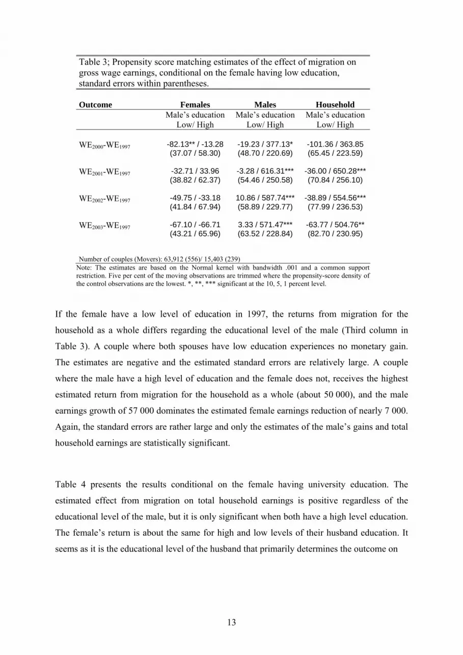
Table 3; Propensity score matching estimates of the effect of migration on gross wage earnings, conditional on the female having low education, standard errors within parentheses. Outcome Females Males Household Male’s education

Low/ High Male’s education

Low/ High Male’s education

Low/ High WE2000-WE1997 -82.13** / -13.28

(37.07 / 58.30)

-19.23 / 377.13* (48.70 / 220.69)

-101.36 / 363.85 (65.45 / 223.59)

WE2001-WE1997 -32.71 / 33.96 (38.82 / 62.37)

-3.28 / 616.31*** (54.46 / 250.58)

-36.00 / 650.28*** (70.84 / 256.10)

WE2002-WE1997 -49.75 / -33.18 (41.84 / 67.94)

10.86 / 587.74*** (58.89 / 229.77)

-38.89 / 554.56*** (77.99 / 236.53)

WE2003-WE1997 -67.10 / -66.71 (43.21 / 65.96)

3.33 / 571.47*** (63.52 / 228.84)

-63.77 / 504.76** (82.70 / 230.95)

Number of couples (Movers): 63,912 (556)/ 15,403 (239)

Note: The estimates are based on the Normal kernel with bandwidth .001 and a common support restriction. Five per cent of the moving observations are trimmed where the propensity-score density of the control observations are the lowest. *, **, *** significant at the 10, 5, 1 percent level.

If the female have a low level of education in 1997, the returns from migration for the

household as a whole differs regarding the educational level of the male (Third column in

Table 3). A couple where both spouses have low education experiences no monetary gain.

The estimates are negative and the estimated standard errors are relatively large. A couple

where the male have a high level of education and the female does not, receives the highest

estimated return from migration for the household as a whole (about 50 000), and the male

earnings growth of 57 000 dominates the estimated female earnings reduction of nearly 7 000.

Again, the standard errors are rather large and only the estimates of the male’s gains and total

household earnings are statistically significant.

Table 4 presents the results conditional on the female having university education. The

estimated effect from migration on total household earnings is positive regardless of the

educational level of the male, but it is only significant when both have a high level education.

The female’s return is about the same for high and low levels of their husband education. It

seems as it is the educational level of the husband that primarily determines the outcome on

13

Table 4; Propensity score matching estimates of the effect of migration on gross wage earnings, conditional on the female having high education. Standard errors within parentheses.

Outcome Females Males Household

Male’s education Low/ High



WE2000-WE1997

65.88/ 41.31 (72.23/ 39.89)

-1.66/ 217.30*** (88.23/ 86.91)

64.23/ 258.61*** (109.39/ 96.12)

WE2001-WE1997

126.53/34.01 (77.79/ 42.32)

-84.27/ 79.28 (94.04/ 62.16)

42.26/ 113.28 (127.03/ 76.68)

WE2002-WE1997

73.78/ 35.87 (77.92/ 47.74)

-24.43/ 140.52** (120.94/ 63.50)

49.35/ 176.39** (140.36/ 80.64)

WE2003-WE1997

60.15/ 101.31** (83.23/ 50.66)

-39.47/ 274.07** (117.59/ 66.26)

20.68/ 375.37*** (141.52/ 84.84)

Number of couples (Movers): 19,200 (251)/ 27,376 (865)


total household earnings. A couple where both spouses have higher education the total

household gain from migration after four years is about 38 000, where of the major part

derives from the effect on the earnings of the male.

The monetary benefit for a male with higher education appears to be dependent on the

educational level of his spouse. A highly educated male living with a highly educated female

receives an increase in earnings that is substantially lower than for those living with low

educated females (27 000 compared to 57 000 four years after the move). For males and

females with a low level of education, the effect on individual earnings is slightly negative or

zero, and the educational level of the spouse does not seem to matter for the size of the return

from migration.

Does migration affect the female share of household income? Table 5 gives the matching

estimates of the effect on females share between 1997 and post-migration shares measured

14

each year from 2000 to 2003. When using the whole sample (first column in Table 5), the

estimated effect from migration is positive but insignificant in three cases out of four. When

the sample is separated by educational level, all estimates pertaining to females with a low

Table 5; Propensity score matching estimates of the effect of migration on the female’s share of total household gross wage earnings, standard errors within parentheses.

Outcome Entire sample

Female low and male low/high

education

Female high and male low/high

education

( ) ( )MF

F

MF

F

WEWEWE

WEWEWE

19971997

1997

20002000

2000

+−

+ .0008

(.0061)

-.0063/-.0061 (.0130/ .0170)

.0347*/ -.0050 (.0185/ .0079)

( ) ( )MF

F

MF

F

WEWEWE

WEWEWE

19971997

1997

20012001

2001

+−

+ .0126 **

(.0064)

.0196/-.0056 (.0134/ .0177)

.0432***/ -.0029 (.0180/ .0085)

( ) ( )MF

F

MF

F

WEWEWE

WEWEWE

19971997

1997

20022002

2002

+−

+ .0025

(.0064) .0019/-.0192

(.0129/ .0177)

.0345*/ -.0065 (.0192/ .0085)

( ) ( )MF

F

MF

F

WEWEWE

WEWEWE

19971997

1997

20032003

2003

+−

+ .0052

(.0066) .0087/-.0181

(.0139/ .0200)

.0347*/ -.0027 (.0195/ .0086)

Number of couples (movers) 125 891 (1 911)

63 912 (556)/ 15,392 (228)

19,188 (239) / 27,333 (822)


level of education are insignificant (second column in Table 5). However, for the sample of

highly educated females married/cohabiting with males having a lower level of education, the

estimates are positive and significant in all four cases (left entries in the third column). For

this sample, the migration seems to increase the female share of total household earnings

around four percentage points. Although most of the estimates in table 5 are not significant,

they are generally in accordance with the hypothesis that spouses education matters for the

effect of migration on the female/male relative share of total household income. There is,

however, no evidence of substantial effects of education on the impact of migration on

females/males relative earnings, except for the sample of highly educated females whose

partners have a low level of education.

To separate the hypothetical effects from education and income on bargaining power, we split

the sample according to whom of the spouses that had higher average earnings over the three

15

years prior to the move (table 6 and 7). For the sample of households with the male as the

principal earner (Table 6), his spouse was the relative winner. The estimated effects of the

change in female share are significant between years of 1997 and 2001, 2002 and 2003 (first

column table 6). The estimates of the change in the female share are positive for all but one

combination of educational levels. The estimates are, however, only significant if the male

has low education. Judging from these estimates, males with low levels of education

experience the largest loss in relative income. There is, nevertheless, no clear cut pattern

indicating that the relative level of education determines the changes in income shares. Given

that the male has a low level of education (left entries in columns 2 and 3 in table 6), the

relative gain for females with a low level of education is close to the estimated gain for

females with a higher education.

Table 6; Propensity score matching estimates of the effect of migration on the female’s share of total household gross wage earnings, conditional on the woman’s share being less than 0.5 in 1995-1997. Standard errors within parentheses.



education


education

( ) ( )MF

F

MF

F

WEWEWE

WEWEWE

19971997

1997

20002000

2000

+−

+

.0072 (.0059)

.0134/ -.0111 (.0132/.0157)

.0292/.0032 (.0190/.0075)

( ) ( )MF

F

MF

F

WEWEWE

WEWEWE

19971997

1997

20012001

2001

+−

+

.0185** (.0061)

.0380***/ -.0025 (.0135/.0157)

.0285/.0112 (.0192/.0080)

( ) ( )MF

F

MF

F

WEWEWE

WEWEWE

19971997

1997

20022002

2002

+−

+

.0112* (.0062)

.0174/ -.0160 (.0129/.0163)

.0419**/.0072 (.0211/.0082)

( ) ( )MF

F

MF

F

WEWEWE

WEWEWE

19971997

1997

20032003

2003

+−

+

.0147** (.0064)

.0197/ -.0045 (.0144/.0172)

.0389*/.0095 (.0202/.0083)

Number of couples (movers) 104 581 (1 522)

52,686 (413)/ 13,925 (203)

14,904 (187)/ 23,336 (719)


In couples where the male was the secondary earner the preceding years (table 7), reallocation

increases his relative share of total earnings. This result holds for all educational combinations

except one. In couples where the female has higher education than the male, she experiences a

larger effect on her earnings than her partner does.

16

In all, we find that the secondary earner receives an increase in the share of total household

earnings as a result of migration. This applies for both sexes, although this effect seems to be

smaller for females than males on average when comparing the first columns in tables 6 and

7. Moreover, in couples where the female has a high level of education and the male does not,

migration increases the female share of household income whether or not she is the principal

earner before migration. Without jumping to conclusions, the results seem to indicate that

initial income is not positively correlated with bargaining power affecting the relative

earnings outcomes from migration.

Table 7; Propensity score matching estimates of the effect of migration on the female’s share of total household gross wage earnings, conditional on the female’s share being equal to or more than 0.5 in 1995-1997. Standard errors within parentheses.



education


education

( ) ( )MF

F

MF

F

WEWEWE

WEWEWE

19971997

1997

20002000

2000

+−

+

-.0381** (.0170)

-.0494/.0148 (.0309/ .0655)

.0712/ -.0563*** (.0527/.0242)

( ) ( )MF

F

MF

F

WEWEWE

WEWEWE

19971997

1997

20012001

2001

+−

+

-.0341* (.0177)

-.0257/-.0180 (.0313/.0694)

.0943/ -.0753*** (.0485/.0266)

( ) ( )MF

F

MF

F

WEWEWE

WEWEWE

19971997

1997

20022002

2002

+−

+

-.0430*** (.0168)

-.0330/-.0322 (.0307/.0702)

.0506/ -.0667*** (.0449/.0258)

( ) ( )MF

F

MF

F

WEWEWE

WEWEWE

19971997

1997

20032003

2003

+−

+

-.0408** (.0177)

-.0254/-.0891 (.0318/.0753)

.0497/ -.0624*** (.0533/.0249)

Number of couples (movers) 21,040 (389) 11,226 (143)/ 1,478 (36)

3,765 (64)/ 4,040 (146)


Summing up the empirical results, our findings indicate that migration affects earnings

positively for the household. However, this applies only for households where the male has a

high level of education. Another finding is that the spouse with the highest level of education

seems to be the relative winner from migration, although this is only significant when the

female has a higher level of education. When the male and the female have unequal levels of

education, the spouse with the lower level of education experience no gain in earnings from

migration.

17

V Conclusion and discussion

Our findings indicate that migration has a positive effect on total household gross wage

earnings. The average effect derives primarily from the large earnings increases among highly

educated males. In general, we find little evidence of positive effects of migration on earnings

among females. However, the education level seems to be positively correlated with the

income gain also among the females, although the estimated effects are relatively small or

statistically insignificant even for the highly educated females.

When examining the change in the female/male share of total household earnings, we find

that the effect of migration is negligible on average. The relative educational level between

spouses does, however, matter for the effect of migration on relative earnings within the

household. Highly educated females coupled with low educated males, experience an increase

in the income share of around four percentage points compared to non-migrants. The largest

negative effect of migration on the female earnings share is found among females with a low

level of education whose male partners are highly educated.

Although not conclusive evidence, we interpret our empirical findings in relation to the

concept of tied migration as follows. The substantial gain in total income among migrating

two-earner households implies that migration ties are not important enough to fully offset

increases in household income as a result of migration. Moreover, tied migration does not

counteract potential income gains to an extent that incurs a decrease in income for the male or

the female. This applies on average for the whole sample.

Disaggregated analysis reveal that education levels affect the gains from migration in terms of

individual earnings, total household earnings and the female share of total earnings. The latter

finding is, however, statistically and economically important only for highly educated females

married/cohabitating with males having a lower level of education. A cautious interpretation

of the results is that they do not speak against the hypotheses that the relative education level

between spouses matters for bargaining power when household location decisions are made.

Being the principal income earner seems not to yield decisive intra-household bargaining

18

power in this context. Our findings indicate that the spouse with the lower income experience

the largest effect of migration on the relative share of total household income.

19

References

Angrist J, 1998. “Estimating the Labor Market Impact of Voluntary Military Service Using Social Security Data on Military Applicants”, Econometrica, 66:2, 249-288.

Axelsson R. and Westerlund O., 1998. “A Panel Study of Migration, Self-Selection and Household Real Income”, Journal of Population Economics, 11: 113–126.

Becker G. A., 1974. “A theory of Social Interactions”, Journal of Political Economy, 82:6, 1063-1094.

Becker G. A., 1981. A Treatise on the Family. Harvard University Press.

Cooke T. J., 2003. “Family Migration and the Relative Earnings of Husbands and Wives”, Annals of the Association of American Geographer, 93:2, 338-349.

Eichler, M. and Lechner, M. 2002. “An Evaluation of Public Employment Programmes in the East German State of Sachsen-Anhalt”, Labour Economics, 9: 2, 143-86.

Greenwood M. J., 1997. “Internal Migration in Developed Countries”, in Handbook of Population and Family Economics, M. R. Rosenweig and O. Stark, editors; Elsevier Science B. V., 1997: 647-711.

Jacobsen J. P. and Levin L. M., 2000. “The effects of internal migration on the relative economic status of women and men”, Journal of Socio-Economics, 29, 291-304.

Lundberg S and Pollak R. A., 1996. “Bargaining and Distribution in Marriage”, Journal of Economic Perspectives, 10:4, 139-158.

Lundberg S. and Pollak R. A., 2001. “Efficiency in Marriage”, NBER working paper 8642, National Bureau of Economic Research, Cambridge, MA, USA.

Mincer J., 1978. “Family Migration Decisions”, Journal of Political Economy, 86, 749-73.

Nakosteen, R. A. and Westerlund, O. 2004. “The Effects of Regional Migration on Gross Income of Labor in Sweden”, Papers in Regional Science, 83:3, 581-595.

20

Nilsson, K., 2000. “Dual University-Graduate Households in Sweden: The Effect of Regional Variations and Migration on Income Equality”, International Journal of Population Geography, 6, 287-301.

Nivalainen, S., 2004. “Determinants of family migration: Short moves vs. long moves”, Journal of Population Economics, 17: 1, 157-175.

Nivalainen, S., 2005. “Interregional Migration and Post Move Employment in Two-earner Families: Evidence from Finland”, Regional Studies, 39:7, 891-907.

Rosenbaum, P. and Rubin, D. 1983. “The Central role of the Propensity Score in Observational Studies for Causal Effects”, Biometrika, 70:1, 41-55.

Samuelson, P. A., 1956. “Social Indifference Curves”, Quarterly Journal of Economics, 70:1, 1-22.

Sandell, S. H., 1977. “Women and the Economics of Family Migration”, The Review of Economics and Statistics, 59:4, 406-414.

Smith, J. and Todd, P. 2005. “Does matching overcome LaLonde’s critique of nonexperimental estimators?” Journal of Econometrics, 125:1-2, 305-353.

Smits J., 2001. “Career Migration, Self-selection and the Earnings of Married Men and Women in the Netherlands”, 1981-93, Urban Studies, 38:3, 541-562.

21

Appendix 1 Individual attributes: Gross wage earnings 1997-2003; in hundreds of Swedish Kronor. Age; in 1997. Child(ren); couple has at least one child below the age of 18 living at home. Small children; couple only has children under the age of seven living at home. Student; individual received study aid for higher education or adult education. Educational level; highest level of education attained by 1997. Sector; sector of work in 1997 according to the Industry code (sni92) as defined by Statistics Sweden. Welfare benefit; family received benefit in 1997. Migration history at least one of the spouses has moved between 1994 and 1997. Regional attributes: Ln extacces; Stockholm; couple lived in Stockholm county in 1997. South of Sweden; couple lived in Skåne or Blekinge county in 1997. Population; total population aged 16-64 in labour market region in 1997.

22

Appendix 2 Variable Logit estimation of migration in

1998 or 1999 Regression on difference in total

household gross income 1997-2000

lnextacc -0,00472 (-1,49)

1,346856 (1,17)

*

befolk97 -4,35E-07 (-5,85)

*** 0,000475 (26,13)

***

reg4dm7 -0,32588 (-4,21)

*** -110,35 (-6,92)

***

lder7 -0,04721 (-8,71)

*** -4,12401 (-3,19)

***

barn97 -0,78396 (-9,7)

*** 564,6162 (25,64)

***

student 0,62409 (5,8)

*** 327,256 (7,35)

***

studentf 0,393793 (4,69)

*** 358,6813 (14,28)

***

social 1,161118 (9,63)

*** -9,87586 (-0,24)

smbarn 0,587022 (9,4)

*** 185,164 (13,1)

***

mig9497 1,736851 (29,14)

*** 35,82998 (1,15)

utbild_3 -0,05596 (-0,59)

1,463503 (0,09)

utbild_4 0,328472 (3,07)

** 130,4683 (6,1)

***

utbild567 0,586044 (6,22)

*** 460,9587 (24,68)

***

utbildf_3 -0,27715 (-2,72)

** 37,43335 (1,89)

*

utbildf_4 -0,1938 (-1,69)

* 148,7138 (6,25)

***

utbild567f 0,184831 (1,83)

* 347,2571 (16,43)

***

sektor_2 -0,27947 (-1,68)

* -169,121 (-5,13)

***

sektor_3 -0,43196 (-6,66)

*** -28,0523 (-1,87)

*

sektor_4 -0,48265 (-4,58)

*** -77,538 (-3,85)

***

sektor_5 -0,2196 (-3,34)

*** 11,70188 (0,76)

_cons -2,1681 (-9,25)

*** -259,193 (-4,43)

***

Note: *** Indicates significant at the 1 percent level; ** indicates significant at the 5 percent level and * indicates significant at the 10 percent level.

23

Documents

Sex and migration: who is the tied mover?