Short-time dynamics of permeable particles in concentrated suspensions

Short-time dynamics of permeable particles in concentrated suspensionsGustavo C. Abade,1 Bogdan Cichocki,1 Maria L. Ekiel-Jeżewska,2,a� Gerhard Nägele,3

and Eligiusz Wajnryb2

1Institute of Theoretical Physics, University of Warsaw, Hoża 69, Warsaw 00-681, Poland2Institute of Fundamental Technological Research, Polish Academy of Sciences, Pawińskiego 5B,Warsaw 02-106, Poland3Institut für Festkörperforschung, Forschungszentrum Jülich, Jülich D-52425, Germany

�Received 14 October 2009; accepted 24 November 2009; published online 4 January 2010�

We study short-time diffusion properties of colloidal suspensions of neutral permeable particles. Anindividual particle is modeled as a solvent-permeable sphere of interaction radius a and uniformpermeability k, with the fluid flow inside the particle described by the Debye–Bueche–Brinkmanequation, and outside by the Stokes equation. Using a precise multipole method and thecorresponding numerical code HYDROMULTIPOLE that account for higher-order hydrodynamicmultipole moments, numerical results are presented for the hydrodynamic function, H�q�, theshort-time self-diffusion coefficient, Ds, the sedimentation coefficient K, the collective diffusioncoefficient, Dc, and the principal peak value H�qm�, associated with the short-time cage diffusioncoefficient, as functions of porosity and volume fraction. Our results cover the full fluid phaseregime. Generic features of the permeable sphere model are discussed. An approximate method byPusey to determine Ds is shown to agree well with our accurate results. It is found that for a givenvolume fraction, the wavenumber dependence of a reduced hydrodynamic function can be estimatedby a single master curve, independent of the particle permeability, given by the hard-sphere model.The reduced form is obtained by an appropriate shift and rescaling of H�q�, parametrized by theself-diffusion and sedimentation coefficients. To improve precision, another reduced hydrodynamicfunction, hm�q�, is also constructed, now with the self-diffusion coefficient and the peak value,H�qm�, of the hydrodynamic function as the parameters. For wavenumbers qa�2, this function ispermeability independent to an excellent accuracy. The hydrodynamic function of permeableparticles is thus well represented in its q-dependence by a permeability-independent master curve,and three coefficients, Ds, K, and H�qm�, that do depend on the permeability. The master curve andits coefficients are evaluated as functions of concentration and permeability. © 2010 AmericanInstitute of Physics. �doi:10.1063/1.3274663�

I. INTRODUCTION

Hydrodynamic properties of suspensions of permeablecolloidal particles moving under creeping flow conditions areof interest not only from a fundamental viewpoint, but alsoin terms of applications. To gain better control on the indus-trial processing of colloids in nondilute dispersions requiresto understand the hydrodynamic interactions �HIs� betweenthe particles, and their influence on transport properties suchas diffusion coefficients or the effective shear viscosity. Ex-amples of permeable colloid suspensions are the so-calledfuzzy-sphere systems consisting of permeable particleswhere the internal structure can change with concentration. Awell-studied system of this kind consists of highly perme-able, cross-linked polymer network particles �PNiPAM mi-crogel spheres� immersed in an organic solvent. The short-time dynamics of this system has been recently studied bydynamic light scattering.1 PNiPAM particles are thermosen-sitive, i.e., they exhibit large and reversible volume changesas a function of temperature.2–6 In fuzzy particle systems, thesuspending fluid can penetrate the particles to an extent de-pending on the radial distance from the particle center.

Another well-studied class of permeable colloids can bedescribed by a simple core-shell model of spherical particleswith a rigid, impermeable spherical core and an outer porousshell. The shell represents the coating of the dry core bysome soft material7–9 such as grafted polymers.10–16 Thecoating can stabilize the particles against irreversible aggre-gation, which otherwise may be induced by the van derWaals attraction in the absence of stabilizing mechanisms.The hydrodynamics in the permeable shell can be describedby the Debye–Bueche–Brinkman �DBB� equation for theflow in an isotropic medium of constant porosity k.17,18 Atthe outer particle boundary between the bulk fluid and per-meable shell, the fluid velocity and hydrodynamic stresschange continuously, whereas at the inner particle interfaceseparating the dry core from the permeable shell, stickboundary conditions are commonly used, unless the interfaceconsists mainly of air. In the latter case it is more appropriateto assume zero tangential stress at this interface and zerorelative radial velocity.19

Notwithstanding the fact that the hydrodynamics ofideal, nonpermeable hard spheres with stick boundary condi-tions at their surface is different from that of fuzzy and core-shell particles, measurements on permeable particles havea�Electronic mail: [email protected].

THE JOURNAL OF CHEMICAL PHYSICS 132, 014503 �2010�

0021-9606/2010/132�1�/014503/17/$30.00 © 2010 American Institute of Physics132, 014503-1

Downloaded 30 Nov 2010 to 148.81.55.51. Redistribution subject to AIP license or copyright; see http://jcp.aip.org/about/rights_and_permissions

http://dx.doi.org/10.1063/1.3274663

http://dx.doi.org/10.1063/1.3274663

been commonly interpreted in terms of an effective hard-sphere radius, and an associated effective volume fraction,with values determined to fit the experimental data either forthe intrinsic shear viscosity,20,21 the particle form factor,21

diffusion coefficients, the static structure factor S�q�, or thehydrodynamic function H�q�. However, there is no theoreti-cal justification of such a procedure. Moreover, depending onthe measured quantity, different values for the effective hard-sphere diameter may be obtained.

The reason why the effective hard-sphere analysis isused so often is that little is known about the HIs in nondi-lute systems of permeable spheres, in particular, regardingtheir influence on diffusion transport properties. In contrastwith this, colloidal suspensions of impermeable neutralspheres and, to a lesser extent, also impermeable chargedspheres have been extensively studied in the past by experi-ment, theory, and simulation. As a result, the short-time equi-librium transport properties in these systems are now wellunderstood even at high densities �see, e.g., Refs. 22–31�.

Note that nonphysical predictions may be made in usingan effective hard-sphere interpretation of permeable par-ticles. For instance, the drag force required to push two per-fectly smooth hard spheres together along their line of cen-ters at constant relative speed grows without bound nearcontact, inversely proportional to the gap distance.32 Differ-ent from this, the nonzero slip of fluid at the outer rim of apermeable particle leads to a nonsingular drag coefficient forzero gap width.33 Thus, two spheres can come in contactduring a finite time what has consequences in the aggrega-tion kinetics of unstable colloidal dispersions.34

Theory and simulation work on hydrodynamically inter-acting colloidal porous particles have been concerned so farmostly with the relative motion of two isolated spheres, andthe calculation of the associated hydrodynamic drag forcesunder creeping flow conditions. The two-sphere drag force atfinite Reynolds numbers, relevant to large noncolloidal par-ticles not considered here, was calculated by Wu et al. usingsimulations.35 The axisymmetric and perpendicular migra-tion of multiple core-shell spheres was studied by Chen33

using a boundary collocation method combined with a lubri-cation analysis. This study quantified the expected increasinginfluence of the HIs with decreasing permeability and thefinite value of the drag force at particle contact.

Little is known theoretically to date about suspension-averaged transport properties in porous-particle systems, inparticular, for nondilute systems. Chen and Cai36 calculatedthe mean sedimentation velocity in a homogeneous, mono-disperse suspension of uniformly porous spheres to first or-der in the volume fraction. They showed that the hydrody-namic hindrance effect on the sedimentation coefficient isweakened with increasing permeability, and that the sedi-mentation velocity is quite sensitive to the direct interactions.For example, addition of a surface charge to the particlesstrongly reduces the sedimentation coefficient, whereasattractive interactions enhance sedimentation. Mo andSangani37 used a multipole expansion method for hydrody-namically interacting porous spheres to obtain numerical re-sults for the average drag force per particle in random and inbcc fixed-bed arrays, and for the high-frequency limiting vis-

cosity of uniformly porous spheres with the equilibrium no-overlap direct interactions. The high-frequency limiting vis-cosity of a suspension of interacting core-shell particles wasalso calculated by Russel et al.,38,39 with an account of thedensity profile of surface-grafted polymers, but with the HIstreated in a lubrication approximation.

On the other hand, there exists an efficient theoreticalscheme to calculate HIs in suspensions, based on solving theStokes equations by the multipole expansion.40–42 Its advan-tage in comparison with other formulations of the Stokesiandynamics is that it can be easily modified to account forvarious hydrodynamic models of the particles. Actually, inthe full many-body theoretical algorithm, specific boundaryconditions at a particle surface enter only through the single-sphere friction coefficients. Those have been evaluated for alarge collection of hydrodynamic models of spherical par-ticles, such as hard spheres with stick boundary conditions,permeable particles, liquid droplets, gas bubbles, particleswith slip-stick boundary conditions, and even core-shellparticles.43–47 This theoretical scheme and the correspondingHYDROMULTIPOLE numerical code are therefore well suitedto describe the hydrodynamics of a variety of particulate sys-tems. An additional advantage is that, in this approach,higher-order multipole moments are taken into account, re-sulting in a strictly controlled precision.

The present paper reports on the first comprehensiveHYDROMULTIPOLE simulation study of short-time diffusionproperties for a suspension of uniformly porous spheres, as afunction of the reduced inverse hydrodynamic screeninglength, x=a /�k, and the volume fraction �. For simplicity,and to highlight the generic influence of porosity using aminimal number of system parameters, we assume thatspheres of radius a interact directly only via the no-overlapcondition. Suspensions at various concentrations are consid-ered, from high volume fractions where many-body HIs arestrong, down to dilute systems. Moreover, x is varied fromsmall values representing highly porous particles to verylarge values where the well-studied limit of nonpermeablehard spheres with stick boundary conditions �hard spheres,for short� is recovered. Using the HYDROMULTIPOLE simula-tion method, numerical results are derived for the hydrody-namic function H�q� as a function of the scattering wave-number q, and for the associated short-time diffusionfunction D�q�, probed in dynamic scattering experiments.These two functions reduce at small q to the short-time sedi-mentation and collective diffusion coefficients, respectively.At large q, both functions asymptote to the short-time �nor-malized� self-diffusion coefficient. Both sedimentation andself-diffusion coefficients are evaluated numerically by a di-rect simulation independent of q.

A key finding of the present study is that an appropri-ately defined reduced hydrodynamic function, h�q�, is to agood approximation equal to the corresponding reducedfunction of nonpermeable hard spheres, independent of thepermeability. Therefore H�q� can be estimated in terms of aporosity-independent hard-sphere master function, and thelimiting values H�q→0� and H�q→��, which do depend onthe porosity. For qa�2, another choice of reduced hydrody-namic function hm�q� is possible, which allows to express

014503-2 Abade et al. J. Chem. Phys. 132, 014503 �2010�


H�q� with a high precision by a porosity-independent hard-sphere master function and the values of H at the first maxi-mum, H�qm�, and in the limit of large q, H�q→��, which dodepend on porosity.

The paper is structured as follows. Section II includesthe theoretical background on the short-time dynamics ofinteracting colloidal spheres and describes our model of po-rous spheres. The essentials of our multipole method and thesimulation procedure are explained in Sec. III. The simula-tion results, their discussion, and comparison with earlierfindings are contained in Sec. IV. The conclusions are givenin Sec. V. In Appendix A, we present the single-particle op-erator of a homogeneously porous sphere used as input inour simulations. A correction used in the extrapolation froma finite-size system to the thermodynamic limit is describedin Appendix B. In Appendix C, we discuss the large-wavenumber behavior of the hydrodynamic function andstructure factor.

II. SHORT-TIME DYNAMICS

A. General definitions

We consider a macroscopically large system of N equalspherical colloidal particles immersed in a Newtonian, qui-escent fluid of shear viscosity �0. At a low Reynolds number,the fluid velocity field, v�r�, and pressure field, p�r�, outsidethe particles satisfy the stationary Stokes equation48

�0�2v − �p = 0, � · v = 0. �1�

For a given configuration X= �R1 , . . . ,RN� of centers offreely rotating spheres, the linearity of the hydrodynamicequations leads to a linear relation between the translationalparticle velocities U= �U1 , . . . ,UN�, and the external forcesF= �F1 , . . . ,FN� that drive the motion of the spheres:

Ui = �j=1

N

�ijtt�X� · F j, i = 1, . . . ,N . �2�

Here, �tt, with the tensor elements �ijtt, is the translational-

translational part of the mobility matrix. It depends on theconfiguration of all the particles in the system, and on thehydrodynamic model for the particles.

Short-time colloidal diffusion properties can be probedby a variety of scattering techniques. In photon correlationspectroscopy and neutron spin echo experiments on fluidlike,isotropic systems, the dynamic structure factor, S�q , t�, is de-termined as a function of scattering wavenumber q and cor-relation time t. On the colloidal short-time scale,49,50 S�q , t�decays exponentially with time according to

S�q,t�S�q�

exp�− q2D�q�t� , �3�

with the q-dependent short-time diffusion function, D�q�, de-fined by the relation,

limt→0

�

�tln S�q,t� = − q2D�q� . �4�

D�q� can be expressed as the ratio

D�q� = D0H�q�S�q�

�5�

of the hydrodynamic function H�q�, and the equilibriumstatic structure factor S�q�=S�q , t=0�.

The statistical-mechanical expression for H�q� in an in-finite isotropic system of mechanically identical colloidalspheres is given by51

H�q� = lim� kBT

ND0�i,j=1

N

exp�iq · Ri�q̂ · �ijtt�X�

· q̂ exp�− iq · R j�� , �6�

where q̂ is the unit vector in the direction of q, and thebrackets represent an equilibrium ensemble average. Here,lim� is a short-hand notation for the thermodynamic limitN→�, V→�, with n=N /V fixed, characterizing a macro-scopic system. To shorten the notation, we do not display thislimit any more. Whenever an ensemble average is consideredin the following, it is tacitly assumed that the thermodynamiclimit has been performed.

The positive valued function H�q� has been nondimen-sionalized by division through the single-particle transla-tional diffusion coefficient, D0, which is probed experimen-tally in ultradilute suspensions where detectable interparticlecorrelations are absent. This coefficient depends on the hy-drodynamic model for the particles. In the special case ofhard spheres with stick boundary conditions, it is given byD0

hs=kBT / �6��0a�.The hydrodynamic function is a measure of the influence

of the HIs on short-time diffusion. It consists of aq-independent self-part and a q-dependent distinct-part,

H�q� =Ds

D0+ Hd�q� . �7�

Here, Ds is the short-time translational self-diffusion coeffi-cient for an isotropic system, given on the colloidal short-time scale by the initial slope of the mean-squaredisplacement,51

Ds = limt→0

1

6

d

dt��R1�t� − R1�0��2 =

kBT

3tr 1

N�i=1

N

�iitt�X�� ,

�8�

with tr denoting the trace operation.In the large-q limit, the distinct part vanishes and H�q�

reduces to Ds /D0. Without HIs, H�q� would be identicallyequal to one, so that any q-dependence reflects the influenceof the HIs. The hydrodynamic function can be interpreted asthe �reduced� short-time generalized mean sedimentation ve-locity in a homogeneous suspension of monodisperse spheressubject to a weak force field collinear with q and oscillatingspatially as cos�q ·r�.23 Consequently, for q→0, the sedi-mentation problem in a uniform force field is recovered, sothat

014503-3 Short-time dynamics of permeable particles J. Chem. Phys. 132, 014503 �2010�


K =U

U0= lim

q→0H�q� =

kBT

3D0tr 1

N�i,j=1

N

�ijtt�X��

irr

, �9�

is the concentration-dependent short-time average sedimen-tation velocity, U, of particles under a uniform force field,normalized by the particle-model dependent sedimentationvelocity, U0, of an isolated particle in the same force field.Because of hydrodynamic long-distance contributions, thelimit q→0 of H�q� is required in the above equation. In therightmost expression, which does not depend on q, the aver-age is taken with respect to the irreducible part of the mobil-ity tensor, without long-distance contributions.52 Alterna-tively, the average can be taken over a periodic cubic cell ofsize L, in the limit of L→�.

The sedimentation coefficient K can be used for a directevaluation of the �short-time� collective diffusion coefficientvia the expression

Dc =D0

S�0�K = lim

q→0D�q� , �10�

where S�0�ª limq→0 S�q� denotes the small-q limit of thestatic structure factor. In contrast with Ds, which is smallerthan D0 for interacting particles, Dc can be substantiallylarger than D0.

Another quantity of interest related to H�q� is the so-called cage diffusion coefficient, defined as the value, D�qm�,of the short-time self-diffusion function D�q� taken at thelocation qm of the principal peak in H�q�. This peak locationcoincides practically with that of the principal peak in S�q�.It is found empirically that D�qm� is the minimal value ofD�q�. The wavelength 2� /qm characterizes the size of thenext neighbor cage around a particle. For hard spheres thiswavelength is roughly equal to the sphere diameter 2a, andwe will see in the following that qma3 �independently ofvolume fraction� also for porous particles.

B. Porous particle model

We assume that the N particles are spheres of the sameradius a, consisting of the same uniform material of constantDarcy porosity �permeability� k. For pore sizes sufficientlysmaller than a, the flow inside the particles can be describedby the Debye-Bueche-Brinkman �DBB� equation

�0�2v − �0�2�v − ui� − �p = 0, � · v = 0, �11�

where �−1=�k is the hydrodynamic screening length, and

ui�r� = Ui + �i � �r − Ri� �12�

is the rigid-body velocity field of a sphere i, with center atposition Ri, that is moving with translational and rotationalvelocities Ui and �i, respectively. The DBB equation de-scribes the pore-sized averaged flow inside a porous particle.To determine the colloid diffusion, the Stokes and DBBequations governing the flow outside and inside the spheres,respectively, must be solved under the conditions that thevelocity v and fluid hydrodynamic stress change continu-ously across the spheres surfaces, and that v goes to zero faraway from the particles. We assume that the particles do notdeform and do not overlap.

The mobility tensor in this porous-particle model de-pends on the reduced inverse hydrodynamic screeninglength, x=� a=a /�k, taken relative to the particle radius a.The single-particle diffusion coefficient, D0, in the poroussphere model is particularly sensitive to x. We will denote itin the following by D0�x� to emphasize its x dependence. Inthe zero permeability limit, x→�, the Stokes–Einstein diffu-sion coefficient, D0��=D0

hs=kBT / �6��0a�, of an isolated,nonpermeable hard sphere is recovered. The ratio of the hy-drodynamic drag on a homogeneously porous sphere relativeto that of a nonpermeable one with stick boundary conditionsis given by17,53

�x� =D0

hs

D0�x�=

2x2�x − tanh x�2x3 + 3�x − tanh x�

. �13�

The function �x� grows monotonically from zero to�x1�=1−x−1+O�x−2� for large x. In terms of �x�, onecan define an effective �hard-sphere� hydrodynamic radius ofa porous particle, aeff�x�=�x� a. For a highly permeablesphere characterized by a small value of x, D0�x� is substan-tially larger than D0, reflecting the low hydrodynamic fric-tion experienced by a strongly permeable sphere. The coef-ficient corresponding to �x� that describes the rotationalmotion of an isolated, homogeneously porous sphere hasbeen derived in Ref. 54 �see, also Ref. 55�. Moreover, thecorresponding first-order virial coefficient for the shear vis-cosity of an ultradilute suspension of uniformly porousspheres in simple shear flow is known since the early workof Debye and Bueche.17

While the single-sphere results are well established andhave been thoroughly tested experimentally, very little isknown about the transport properties of interacting porousspheres. Chen and Cai36 calculated the first virial coefficientof the sedimentation coefficient, �K�x��0, with

K�x;�� = 1 − �K�x�� + O��2� , �14�

for various values of x. Here, �= �4� /3�na3 is the volumefraction for the particle density n. They found that �K�x�becomes larger with increasing x, in accord with the moregeneral expectation, confirmed by our simulations, that Kbecomes smaller with increasing x for any value of �, notjust small ones. This reflects the growing strength of the HIsfor decreasing porosity. It should be born in mind that theenhancement of the mean sedimentation velocity, U�x ;��,with decreasing x, is due to two contributions: the first one isthe enhancement of the single particle sedimentation velocityU0�x��D0�x� and the second stems from the decreasingstrength of the HIs acting between the particles.

For later use in our discussion, we quote a few analyticresults known about the short-time properties of imperme-able monodisperse hard spheres. Truncated virial expansionexpressions have been derived by Cichocki et al.,56,57

Dshs/D0

hs = 1 − 1.832� − 0.219�2 + O��3� , �15�

Uhs/U0hs = 1 − 6.546� + 21.918�2 + O��3� , �16�



Dchs/D0

hs = 1 + 1.454� − 0.45�2 + O��3� . �17�

The quoted expressions include HIs up to the three-bodylevel and account for lubrication corrections.

For a suspension of nonpermeable hard spheres with ar-bitrary values of �, numerical results for the sedimentationand diffusion coefficients, and the hydrodynamic function,are known from hydrodynamic force multipole calculations22

and fluctuating lattice Boltzmann simulations23–25 pioneeredby Ladd, and from the accelerated Stokesian dynamics simu-lation schemes developed by Brady and co-workers.26–28

These simulation studies extend up to the freezing volumefraction of hard spheres, partially even up to random closedpacking. A comprehensive discussion of the short-time prop-erties of neutral and charge-stabilized hard spheres includingmany simulation, analytic, and empirical results is given inRef. 30. The following empirical result is worth mentioninghere: The peak height of Hhs�q�, attained at q=qm, is givenwith a good accuracy by the linear form,30

Hhs�qm� = 1 − 1.35� , �18�

valid for concentrations up to the freezing value.

III. MULTIPOLE METHOD

A. Theoretical scheme

In this work, a suspension is modeled by a system of Nparticles in a periodic cell, with periodic boundary conditionsimposed on the flow. For a multipolar description of the HIsbetween the suspended particles, the fluid flow problem isformulated in the induced force picture,58–60 where the pres-ence of the particles immersed in the fluid is accounted forby a density fi�r� of forces exerted by a particle i on the flow,introduced as a source term in the right hand side of theStokes Eq. �1� as follows:

��2v − �p = − �i=1

N

fi�r�, � · v = 0. �19�

In this picture, the equations describing the fluid motion areextended to the whole space including the interior of theparticles. For a suspension of hard spheres with no-slipboundary conditions, the force density is concentrated on theparticle surfaces and the rigid body motion of the particlesmay be interpreted as a fictitious fluid flow for �r−Ri� a,which satisfies the Stokes Eq. �1�. In case of permeable par-ticles the force density is spread throughout the interior ofthe spheres, in such a way that the DBB Eq. �11� is satisfied,and the fluid velocity and stress are continuous at the particlesurface.

If a single particle i, translating and rotating with thelocal velocity field ui�r�, specified in Eq. �12�, is immersedin an incident fluid flow vin, it resists the flow, exerting on itthe density of forces fi, which depends linearly on vin−ui as

fi = Z0�i��ui − vin� . �20�

Here, Z0�i� is an integral operator, referred to as the one-particle friction. Its kernel is nonzero only inside the particlevolume Vi, including its boundary. The resistance Z0�i� de-pends on the particle porosity and, more generally, on the

hydrodynamic model of the interior of the particle and itsboundary.

The one-particle friction operator Z0�i� and the Greenintegral operator related to Eq. �19� are the essential quanti-ties needed to evaluate HIs between many particles.40 In anunbounded system, the fluid flow incident to the particle i isa superposition of an ambient flow v0, created by externalsources in the absence of particles, and the fluid flows gen-erated by all the other particles j� i,

vin�r� = v0�r� + �j�i

N � T�r,r�� · f j�r��dr�,

for r � Vi and r� � Vj , �21�

where T is the Green integral kernel for an unbounded fluid,i.e., the Oseen tensor T0.48

The relation �20� for the incident flow �21� can be writ-ten in a compact form as

fi = Z0�i��ui − v0 − �j�i

N

G�ij�f j� , �22�

where G�ij� is an abbreviated notation for the Green opera-tors in Eq. �21�, describing the velocity field incidenton particle i and induced by a force density on anotherparticle j.

By applying Z0−1�i� to both sides of Eq. �22�, the follow-

ing system of integral equations is obtained, each one validinside a particle volume Vi,

ui − v0 = �j�i

N

G�ij�f j + Z0−1�i�fi, i = 1, . . . ,N . �23�

The first contribution on the right hand side of Eq. �23�,discussed above, does not depend on a hydrodynamic modelof the particles. The second term at the right hand side of Eq.�23� describes the contribution to the velocity of particle ifrom the induced forces located on the same particle i. Thiscontribution is described in terms of the inverse one-particlefriction operator Z0

−1�i� and it depends on the hydrodynamicmodel of the particle. For the porous particles investigated inthis work, the fluid does not stick to their surfaces and Z0�i�is different from the case of hard spheres.

To find the induced force densities, the system of inte-gral Eq. �23� is transformed into an algebraic one by the useof projection on �and expansion in� spherical multipole func-tions �see Refs. 61–63 for details�. The multipole indices l,m, and � take the values l=1,2 ,¯, m=−l , . . . ,+l, and�=0,1 ,2. This leads to an algebraic system of equations,written succinctly in the form

c = �Z0−1 + G�f , �24�

where the infinite dimensional vectors c and f of the velocityand force multipoles consist of the coefficients resultingfrom the projection of the velocity field ui−v0 and the forcedensity fi onto subsequent spherical multipole functions cen-tered at particle i=1, . . . ,N. After projecting onto the multi-pole functions, the operators Z0

−1 and G become infinite di-mensional matrices. Their application to the vector f involvessummation over the multipole indices and the particle labels.



The formal solution of Eq. �24� for f is given by

f = �Z0−1 + G�−1c . �25�

Therefore, for porous particles the relation �25� has the sameform as for hard spheres, with the same Green function Gbut a different single-particle friction Z0. The multipole ele-ments of Z0 for porous particles43,44 are shown explicitly inAppendix A as functions of the permeability.

In numerical computations, the infinite matrices Z0 andG are truncated at a multipole order L,41 such that only ele-ments with l L are taken into account. The truncated matrixZ0

−1+G is then inverted, and the force multipoles f are deter-mined. To speed up the convergence of the multipole expan-sion, the grand friction matrix �Z0

−1+G�−1 is corrected forlubrication effects, which are important if particles are closeto each other.56,64,65 The multipole moments with indicesl=1 and �=0 correspond to the spherical components offorces and translational velocities. Moments with indicesl=1 and �=1 correspond to torques and rotational velocities.The solution of Eq. �25� yields force multipoles of all ordersif translational and rotational velocities of the particles andthe external flow v0 are given. The mobility problem of find-ing translational and rotational velocities for known forcesand torques acting on the particles, in the absence of externalflow, requires the invertion of the matrix �Z0

−1+G�−1, butonly in the space spanned by the multipole functions withindices l=1 and �= �0,1�. According to this procedure,40 thetranslational-translational mobility matrices �ij

tt are evalu-ated, which are needed to determine the hydrodynamic func-tion.

We emphasize that the single-particle operator Z0 is theonly object that must be changed when different hydrody-namic models for the particle interior and boundary condi-tions at its surface are considered. The basic Eq. �25� remainsthe same, and so does the operator G which, as the propaga-tor of the HIs, depends only on the properties of the suspend-ing fluid and its boundaries. Further insight into the advan-tages of separating off the single-particle friction may beobtained by expressing the solution of the many-body HIs interms of the scattering series.40

For the periodic system considered in this work, themain structure remains the same as described above for anunbounded fluid. The difference is that for i� j, the Greenoperator G�ij� has now the Hasimoto tensor TH �Ref. 66� asits kernel. In addition, there appears a self-part G�ii�, withTH−T0 as its kernel, which accounts for propagation due toall the periodic images.42 In this approach, the fluid backflowis taken into account in such a way that we are in the frameof reference, in which the suspension velocity, averaged overthe periodic cell, is exactly equal to zero.67 The total forceexerted by all the particles on the fluid is compensated by thepressure gradient.

Finally, it is important to point out that, in the mutipolemethod, the grand friction matrix �Z0

−1+G�−1 is not pairwiseadditive. We fully take into account many-body HIs betweenthe particles in the periodic cell, without any approximations.Moreover, we apply the lubrication correction, which speedsup the convergence of the multipole expansion and results in

a very high accuracy of our computations in the whole rangeof volume fractions, including very concentrated systems.

B. Numerical computations

The essential steps in the evaluation of HIs, outlinedabove, have been implemented in the well-established nu-merical code called HYDROMULTIPOLE;56 the new elementadded in this work is the one-particle operator Z0 for porousparticles. Within this scheme, matrix inversions are carriedout by use of Cholesky factorization,68 so that the fullN-particle mobility matrix �ij

tt is evaluated. Then, Eq. �6� isused to determine the hydrodynamic function HN�q�, whichis the N-particle counterpart of H�q�.

In our computations, the averaging is performed overequilibrium configurations of N=256 particles in a periodi-cally replicated cubic simulation cell. This procedure is de-noted as �¯ pbc. Equilibrium means here that the N-particledistribution function is equal to one for nonoverlapping par-ticles and zero elsewhere �the standard hard-sphere distribu-tion�. A set of independent hard-sphere configurations usedin the equilibrium averages for H�q� and U was created usingBrownian dynamics simulations and a condensation tech-nique. The results were obtained by averaging over at least100 independent random configurations for each value of xand �.

The function HN�q� is calculated for wavenumbers qconsistent with the periodic boundary conditions imposed tothe simulation cell of length L and given by the magnitudeof the wavevectors q=2��nx ,ny ,nz� /L, with the integernx , ny , nz such that �nx

2+ny2+nz

2�45. The hydrodynamicfunction HN�q� is calculated by averaging over the vectors ofthe same magnitude q. It depends on the number of particlesin the periodic cell and needs to be extrapolated to N→�.

To allow for simulations of larger systems, with N ex-ceeding 1000, an accelerated version of the HYDROMULTI-

POLE code, called FAST HYDROMULTIPOLE, has beendeveloped.69 In the FAST HYDROMULTIPOLE code, the speedof calculation is improved by applying an iterative method tosolve the large system of Eq. �24� for the force multipolemoments. Further improvement is achieved by use of the fastmultipole algorithm70 to construct the matrix G of propaga-tors in sparse form, so that matrix-vector products involvingG require O�N� operations only.

In the fast multipole method, the full mobility matrix �tt

is not calculated. Instead, the fast method provides the solu-tion of the translational mobility problem in the form of aresponse velocity vector U= �U1 , . . . ,UN� to applied forcesF= �F1 , . . . ,FN�. Therefore, the N-particle hydrodynamicfunction HN�q� is evaluated according to

HN�q� =kBT

ND0��

i=1

N

q̂ · Ui�q�exp�iq · Ri� pbc, �26�

where Ui�q� is the ith particle response to spatially periodicexternal forces F= �F1�q� , . . . ,FN�q�� with

F j�q� = q̂ exp�− iq · R j� . �27�

As it has been already mentioned in Sec. II, here we have thepicture of H�q� being a short-time generalized sedimentation



coefficient for a homogeneous suspension of monodisperseparticles subject to a weak, spatially sinusoidal force collin-ear with q. In particular, the fast-multipole code is very ef-ficient in evaluating the hydrodynamic function at q=0, i.e.,for the sedimentation coefficient expressed by Eq. �9�.

In simulations of homogeneous bulk suspensions, peri-odic boundary conditions effectively minimize surface ef-fects, but, as the result of long-range HIs, HN�q� exhibits astrong system-size dependence and measurably deviatesfrom its infinite-system counterpart, H�q�, even if N is notsmall. Simulations are performed for a finite value of N,therefore a finite-size correction from HN�q� to H�q� has tobe evaluated. We extrapolate to the thermodynamic limit us-ing the following expression, valid for N→�,

H�q� = HN�q� + 1.76S�q��0

�eff�x,��/N�1/3, �28�

which, for q→0 and q→�, respectively, includes the finite-size corrections of U and Ds as limiting cases. In this equa-tion, HN�q� is corrected by a term proportional to �� /N�1/3.The correction formula was initially proposed by Ladd in theframework of lattice Boltzmann simulations of colloidal hardspheres,22–24 and subsequently applied successfully to non-permeable charge-stabilized spheres,29,30 and in the frame-work of sedimentation also to porous spheres and drops.37 Itrequires as input the static structure factor S�q�, and the sus-pension effective high-frequency shear viscosity �eff�x ,��.

In this work the structure factor S�q� has been calculatedby use of the Verlet–Weis correction to the Percus–Yevickexpression �VW-PY�.71,72 The VW-PY expression is spe-cially useful in predicting S�q� in the low-q region, which isinaccessible to simulations of finite systems. Apart from thelow-q limit, the structure factor extracted from the hardsphere configurations used in our simulations practically co-incides with the VW-PY predictions in the whole range ofvolume fractions explored.

The suspension effective high-frequency shear viscosity�eff�x ,�� is evaluated by direct fast-multipole simulations, if� and x are small. For larger � or x, the fast multipolemethod is used for N=256,512,1024 to estimate numeri-cally the slope of the linear dependence of H�q� on N−1/3,and to show that it practically does not depend on q. Thedetails of the extrapolation procedure are described inAppendix B. A rigorous theoretical derivation of Eq. �28� isstill an open problem, which will be addressed elsewhere.

Finally, we comment on the precision of our simulations.The accuracy of the standard HYDROMULTIPOLE is controlledby changing the multipole truncation order L. As remarked inRefs. 41 and 63, accurate calculations must be performed atleast at L=3 to account for all long range contributions.Therefore, generically we use L=3. The accuracy of the FAST

HYDROMULTIPOLE is controlled by L and by an additionaltruncation order L� ��L�, discussed in Ref. 69. To evaluatethe extrapolation N→�, we truncate the multipole expan-sions at L=3 and L�=3.

For small wavenumbers q, large x and large volume frac-tions �, precision of the Cholesky multipole method with thetruncation at L=3 deteriorates up to 10% and an extrapola-tion to larger values of L is needed. First, the hydrodynamic

function is evaluated by the fast-multipole method withL=3,5 for N=64,256 particles in the periodic cell and it isshown that the ratio of values corresponding to L=3 andL=5 very weakly depends on N. Next, computations are per-formed with the Cholesky method for L=3,4 ,5 ,6 at asmaller number of particles N=64. It is found thatL=6 is sufficient, because it gives practically the same re-sults as L=5. Then, we calculate the ratio of the H�q�-valuesat L=3 and L=6, and we use it to extrapolate from L=3 toL=6 all the data previously obtained for the hydrodynamicfunction H�q�. The resulting accuracy of the multipole trun-cation is better than 1% at low values of q, and better than0.5% for moderate and large values of q.

Summarizing, we proceed as follows:

�i� Compute the finite-system function HN�q� by theCholesky multipole method with periodic boundaryconditions; ensemble average over equilibrium con-figurations of nonoverlapping particles.

�ii� Calculate the infinite-system function H�q� by cor-recting HN�q� for implicit finite-size effects with thefast-multipole method, as described in Appendix B.

�iii� Correct for the multipole truncation to reach an accu-racy not worse than 1% at low q and not worse than0.5% at larger wavenumbers.

IV. RESULTS

We present simulation results for H�q�, and for the self-diffusion and sedimentation coefficients of porous spheresusing inverse permeabilities x=3, 5, 10, 30, 50, 100, and ��hard spheres�, and volume fractions in the fluid regime se-lected as �=0.05, 0.15, 0.25, 0.35, and 0.45. The resultshave been obtained using the method and procedures de-scribed in the previous section. Recall that the quantities in-troduced in Sec. II have been nondimensionalized by divi-sion through the infinite-dilution single-particle diffusioncoefficient D0. For the present model of uniformly permeablespheres, D0�x� is a function of the single parameter x thatquantifies the degree of permeability. In Table I, D0�x� iscompared with the hard-sphere analog, D0

hs, by listing thesingle-sphere reduced drag coefficient, �x�=D0

hs /D0�x�,evaluated according to Eq. �13�, for the permeabilities con-sidered in our simulations. This table illustrates the basichydrodynamic behavior of the porous particles with the spe-cific values of x used in our simulations. We recall that �x�is the effective hydrodynamic radius of the porous particle,measured relative to its geometric radius a. In typical experi-mental systems of core-shell particles with a thick permeableshell of grafted polymer chains, x�20–30.15

TABLE I. Single-sphere reduced drag coefficient, �x�=D0hs /D0�x�, quoted

in Eq. �13�.

x 3 5 10 30 50 100 �

�x� 0.6013 0.7634 0.8880 0.9651 0.9794 0.9899 1.0000



A. Hydrodynamic function

In Fig. 1, our simulation results for the hydrodynamicfunction, H�q�, are displayed for various values of the re-duced inverse hydrodynamic screening length x, for a diluteand an intermediately concentrated system. With increasingx, i.e., decreasing permeability, and a fixed value of �, H�q�becomes smaller for all values of q. This reflects the decreasein the generalized, q-dependent sedimentation coefficientH�q� when the strength of the HIs is increased by making theparticles less permeable. We further notice from this figurethat changing x does not affect the location, qm, of the prin-cipal peak in H�q�. The principal peak location, qm, coincidespractically with that of the static structure factor. The latterlocation is independent of the HIs since S�q� is a genuinestatic equilibrium property. Notice further that the oscilla-tions in H�q� become stronger with increasing concentration.

Whereas both H�q�qm�K and H�qqm�Ds /D0 de-crease with increasing �, for any value of x, documentingthus the expected decline of the sedimentation and self-diffusion coefficients with increasing concentration, the�-dependence of H�qm� changes qualitatively as a functionof x, as shown in Fig. 2 and Table II. For highly permeable

particles where x 3, H�qm� increases monotonically withincreasing �, akin to what is observed in dilute, low-salinitysuspensions of strongly charged, nonporous spheres.29 Forx5–10, there is even a small nonmonotonicity observablein the density dependence. At larger permeabilities x�20,H�qm� declines monotonically in �. The strongest declinetakes place for x→�. This decline agrees very well with thelinear density form quoted in Eq. �18� with the same coeffi-cient 1.35.

B. Reduced hydrodynamic functions

Consider the reduced hydrodynamic function

h�q� =H�q� − H��H�� − H�0�

, �29�

with H��=Ds /D0 and H�0�=K. It is defined such thath�q→��=0 and h�q→0�=−1, with its overall q dependenceresembling that of the original H�q�. Notice here also thath�q�=Hd�q� / �Hd�0��, where Hd�q� is the distinct part of thehydrodynamic function introduced in Eq. �7�. It should bekept in mind that h�q� is also a function of � and x. Ingeneral, Ds /D0�K for nonzero �, so that h�q� is positivewhenever H�q�−Ds /D0=Hd�q��0. Our numerical resultsfor h�q�, covering the range from highly porous to nonper-meable spheres with stick boundary conditions, and from

0 2 4 6 8 100.7

0.8

0.9

1

qa

H(q

)

φ=0.05

0 2 4 6 8 100

0.2

0.4

0.6

0.8

1

1.2

qa

H(q

)

φ=0.35

(b)

(a)

FIG. 1. Simulation results for the hydrodynamic function H�q� forx=3,5 ,10,30,50,100,� �from top to down�. Top figure: �=0.05. Bottomfigure: �=0.35.

0 0.1 0.2 0.3 0.40.3

0.4

0.5

0.6

0.7

0.8

0.9

1

1.1

1.2

1.3

H(q

m)

φ

x=3

x=5

x=10

x=30

x=50

x=100

x=∞

FIG. 2. Hydrodynamic function principal peak value, H�qm�, as a functionof volume fraction, for various permeabilities as indicated. The simulationpoints are linked by spline fits to guide the eye.

TABLE II. Principal peak value, H�qm�, of hydrodynamic function for dif-ferent values of x and �.

x

�

0.05 0.15 0.25 0.35 0.45

3 1.002 1.018 1.050 1.106 1.2085 0.990 0.982 0.989 1.015 1.08710 0.968 0.916 0.874 0.846 0.84830 0.946 0.843 0.751 0.658 0.58650 0.940 0.825 0.721 0.610 0.519100 0.936 0.812 0.697 0.572 0.462� 0.933 0.797 0.663 0.527 0.396



dilute to concentrated systems, are displayed in Fig. 3.The first key finding in our study, demonstrated by this

figure, is that h�q� remains nearly independent of the perme-ability for all values of q. There are some slight variations inh�q� when x is changed, and these are most visible in theamplitudes of the oscillations in h�q� that grow with increas-

ing x, and also in the small-q region located to the left of theprincipal peak in h�q�. The principal peak, h�qm�, of h�q�attains its largest value when x→�.

Since h�q� is only weakly dependent on x, it can beapproximated by the hard-sphere reduced hydrodynamicfunction,

0 2 4 6 8 10

−1

−0.5

0

0.5

qa

h(q)

φ=0.05

x=3

x=5

x=10

x=30

x=50

x=100

x=∞

0 2 4 6 8 10

−1

−0.5

0

0.5

qa

h(q)

φ=0.15

x=3

x=5

x=10

x=30

x=50

x=100

x=∞

0 2 4 6 8 10

−1

−0.5

0

0.5

qa

h(q)

φ=0.25

x=3

x=5

x=10

x=30

x=50

x=100

x=∞

0 2 4 6 8 10

−1

−0.5

0

0.5

qa

h(q)

φ=0.35

x=3

x=5

x=10

x=30

x=50

x=100

x=∞

0 2 4 6 8 10

−1

−0.5

0

0.5

qa

h(q)

φ=0.45

x=3

x=5

x=10

x=30

x=50

x=100

x=∞

(b)(a)

(c) (d)

(e)

FIG. 3. Reduced hydrodynamic function h�q�, for values of x and � as indicated.



h�q� hhs�q� . �30�

Accordingly, the hydrodynamic function is well approxi-mated by

H�q;x� �Ds�x�D0�x�

− K�x��hhs�q� +Ds�x�D0�x�

, �31�

where the additional �-dependence of the various quantitieshas not been displayed for brevity. While we confirmed thevery weak dependence on x explicitly for uniformly perme-able spheres only, we expect that the dependence of h�q� onpermeability remains very weak also for a more complexhydrodynamic structure of a particle, such as for the core-shell model.

Recall that the common principal-peak location, qm, ofH�q� and h�q� is practically that of the S�q� of hard spheres,so that it is independent of the permeability. Quite remark-able is the low x-sensitivity of the peak value, h�qm�, of thereduced hydrodynamic function h�q�, in particular, since thepeak, H�qm�, of the original H�q� varies strongly with x �seeagain Fig. 2�. The explicit dependence of h�qm� on � and x isshown in Fig. 4. In the wide range of considered porosities,3 x �, the value of h�qm� changes by less than 20%.

A careful analysis of our results for h�q� in Fig. 3 sug-gests that a more accurate description can be obtained if asecond reduced hydrodynamic function, hm�q�, is introduced,now with the use of H�qm� rather than H�0�,

hm�q� =H�q� − H��

H�qm� − H��=

Hd�q�Hd�qm�

. �32�

By definition, hm�qm�=1, independently of x and �. Figure 5demonstrates that for wavenumbers qa�2, including theprincipal peak region of the hydrodynamic function, hm�q� isinsensitive to x. A significant x-dependence is observed onlyat small-q values near to and in the hydrodynamic regime,where H�q�K. The coefficient K depends strongly on x, asit will be discussed in the next section.

We have here the remarkable finding that for qa�2, the

hydrodynamic function H�q� is determined with a high pre-cision by its principal peak value, H�qm�, and H��=Ds /D0,with the q-dependence characterized by hm

hs�q�. Explicitly,

H�q;x� �H�qm;x� −Ds�x�D0�x�

�hmhs�q� +

Ds�x�D0�x�

, for qa � 2.

�33�

We note finally that the oscillations in H�q�, and in the asso-ciated reduced functions h�q� and hm�q�, are growing withincreasing particle concentration.

C. Hydrodynamic function at low wavenumbers

After completing the analysis of the hydrodynamic func-tion for wavenumbers qa�2, we now focus on small wave-numbers, qa 2. We start with q=0, in evaluating the sedi-mentation and collective diffusion coefficients. Table IIIincludes our numerical results for the sedimentation coeffi-cient K�x ;��. The plots are given in Fig. 6�top�.

Since the major effect of permeability is to weaken theHIs, K decreases faster with increasing concentration whenthe permeability is decreased. Nonpermeable spheres sedi-ment most slowly, for the two reasons that the influence ofthe HIs is strongest, and that the single-particle diffusioncoefficient is smaller than for permeable ones. The�-dependence of K, for x=�, agrees well with earlier resultsfor the sedimentation coefficient of nonpermeable hardspheres obtained by Ladd using a force multipole method.22

From Eq. �16� for hard spheres, it follows that O��2� correc-tions are contributing significantly already for �=0.05. Forthis reason, the simulation points in the figure have beenconnected by solid lines using a spline fit. The slopes of thesolid lines for x=� and x=10 agree well with the dashedlines, corresponding to the first-order virial results for x=�and x=10 derived by Batchelor73 and Chen and Cai,36 re-spectively.

The normalized collective diffusion coefficient, Dc /D0,follows from Eq. �10�, if K is divided by S�0�, with the lattergiven with a high accuracy by the Carnahan–Starling ana-lytic expression, S�0�= �1−��4 / ��1+2��2+�3��−4��. Theresult is plotted in Fig. 6�bottom�. Notice the weak�-dependence of Dc for nonpermeable spheres.

Since S�0� in our model is independent of x, the mono-tonic rise of Dc /D0 with increasing � is more pronouncedfor more permeable particles. We point out that Dc depictedin Fig. 6�bottom� is a short-time quantity which at larger

TABLE III. Sedimentation coefficient K as a function of x and �.

x

�

0.05 0.15 0.25 0.35 0.45

3 0.850 0.641 0.511 0.430 0.3785 0.803 0.536 0.376 0.281 0.22110 0.762 0.452 0.275 0.173 0.11430 0.736 0.399 0.217 0.117 0.061850 0.731 0.389 0.206 0.108 0.0542100 0.727 0.382 0.199 0.101 0.0492� 0.724 0.377 0.192 0.0949 0.0448

0.1 0.2 0.3 0.40

0.2

0.4

0.6

0.8h(

q m)

φ

x=3

x=5

x=10

x=30

x=50

x=100

x=∞

FIG. 4. Reduced hydrodynamic function principal peak value, h�qm�, as afunction of volume fraction, for various permeabilities as indicated. Thesimulation points are linked by spline fits to guide the eye.



concentrations, where many-body HIs are active, should bedistinguished from the long-time collective diffusion coeffi-cient. The latter is affected by memory �dynamic caging�effects and is also referred to as gradient diffusion coefficientmeasurable in a macroscopic diffusion experiment. The val-

ues taken by the long-time coefficient in dense systems aresmaller than the ones for Dc, but the difference is commonlyquite small.74

For small wavenumbers, qa 2, the reduced hydrody-namic function hm�q� deviates by up to 20% from the hard-

0 2 4 6 8 10

−8

−6

−4

−2

0

2

qa

h m(q

)φ=0.05

x=3

x=5

x=10

x=30

x=50

x=100

x=∞

0 2 4 6 8 10−6

−4

−2

0

2

qa

h m(q

)

φ=0.15

x=3

x=5

x=10

x=30

x=50

x=100

x=∞

0 2 4 6 8 10−4

−2

0

2

qa

h m(q

)

φ=0.25

x=3

x=5

x=10

x=30

x=50

x=100

x=∞

0 2 4 6 8 10

−2

−1

0

1

qa

h m(q

)

φ=0.35

x=3

x=5

x=10

x=30

x=50

x=100

x=∞

0 2 4 6 8 10−2

−1

0

1

qa

h m(q

)

φ=0.45

x=3

x=5

x=10

x=30

x=50

x=100

x=∞

(b)(a)

(c) (d)

(e)

FIG. 5. Reduced hydrodynamic function, hm�q�, for values of x and � specified in the plots.



sphere master curve when x is decreased down to x=3, asshown in Fig. 5. The q-dependence of hm�q� in this rangewill now be discussed. For qa 1, it is well approximated byhm�q�=hm�0�+A�qa�2, with the coefficient A given inTable IV for different � and x. As illustrated in Fig. 7, for1 qa 2 the linear approximation in �qa�2 is not sufficient,but hm�q� is well approximated if also the �qa�4 term is takeninto account,

hm�q� hm�0� + A�qa�2 + B�qa�4. �34�

Values for the coefficient B are listed in Table IV. For alarger volume fraction, ��0.35, B is practically independentof x.

D. Self-diffusion coefficient

In our simulations, Ds /D0 is determined by calculatingthe trace of the translational-translational mobility matrix ac-TABLE IV. Coefficients A and B in Eq. �34�, as functions of x and �.

x

�

0.05 0.15 0.25 0.35 0.45

A3 2.74 1.07 0.43 0.178 0.0765 2.68 1.01 0.39 0.165 0.06910 2.45 0.89 0.34 0.139 0.05630 2.06 0.74 0.27 0.105 0.04350 1.97 0.70 0.24 0.093 0.039100 1.91 0.66 0.22 0.084 0.036� 1.79 0.61 0.20 0.076 0.029

B3 �0.184 0.000 0.031 0.021 0.0115 �0.178 0.007 0.033 0.022 0.01210 �0.144 0.022 0.038 0.023 0.01230 �0.084 0.037 0.042 0.023 0.01150 �0.072 0.043 0.043 0.024 0.011100 �0.062 0.046 0.044 0.023 0.011� �0.060 0.055 0.046 0.023 0.011

0 0.1 0.2 0.3 0.40.2

0.4

0.6

0.8

1

Ds/D

0

φ

x=3

x=5

x=10

x=30

x=50

x=100

x=∞

FIG. 8. Self-diffusion coefficient, Ds /D0, for permeabilities as indicated.The simulation points are connected by spline fits to guide the eye.

0 0.1 0.2 0.3 0.40

0.2

0.4

0.6

0.8

1K

φ

x=3

x=5

x=10

x=30

x=50

x=100

x=∞

0 0.1 0.2 0.3 0.41

3

5

7

9

11

13

Dc/D

0

φ

x=3

x=5

x=10

x=30

x=50

x=100

x=∞

(a)

(b)

FIG. 6. Sedimentation coefficient �top� and collective diffusion coefficient�bottom� as a function of volume fraction for different permeabilities asindicated. The simulation points are connected by spline fits. The dashed redand blue straight lines are, respectively, the first-order virial expansion re-sults for nonpermeable hard spheres, Khs=1–6.546� �Ref. 73�, and stronglypermeable particles where K=1–5.5�, for x=10 �Ref. 36�.

0 0.5 1 1.5 2 2.5 3 3.5

−1

0

1φ=0.45

qa

h m(q

)

FIG. 7. Low-wavenumber dependence of the reduced hydrodynamic func-tion hm�q� at �=0.45, for permeable particles with x=3 �black solid line�and hard spheres with x=� �red solid line�, in comparison with the polyno-mial approximation in Eq. �34�. The approximation hm�0�+A�qa�2 �dashedlines� is sufficient for qa 1. For qa 2, the term �qa�4 has to be taken intoaccount �dashed-dotted lines�.



cording to Eq. �8�. The results are documented in Fig. 8 andTable V. As one notices from Fig. 8, Ds /D0 decays mono-tonically in �, and its decay is faster for less permeablespheres. The �-dependence of Ds�x=�� agrees well with ear-lier data gained by other numerical methods.22,26,30

The precise values of Ds /D0 listed in Table V are usednow to discuss the accuracy of alternative ways of estimatingthe self-diffusion coefficient, which are of help to extractDs /D0 from experimental data. Suppose that, in a scatteringexperiment, H�q� is measured up to, say, qa 8, which isroughly the location of its third minimum. Then, Ds can beaccurately determined by a least-squares fit of the large-qasymptotic form of H�q�, to the data of H�q�, in the range,e.g., of 4 qa 8. Details of this method are given inAppendix C. With this procedure, Ds /D0 is determined withan absolute error of 0.001 or smaller.

Pusey75 suggested and underpinned experimentally thatself-diffusion can be probed in a dynamic light scatteringexperiment performed at wavenumbers, q��qm, whereS�q��=1, on assuming that DsD�q�� is valid approxi-mately. In a light scattering experiment, the smallest of theseq� �denoted as q1

�� is usually attainable. In Appendix C, it isexplained that this approximation works well, since H�q� andS�q� share a similar large-q asymptotic form, differing onlyin the expansion coefficients. Asymptotic considerations arealso used to estimate the accuracy of the approximation.

Using the HYDROMULTIPOLE code, we demonstrated thatPusey’s method to determine self-diffusion is efficient alsofor permeable particles, for any degree of permeability, whenq1

� or the next larger q� �denoted as q2�� are used. This can be

seen from Table VI which includes values for Ds /D0 ob-tained by direct simulation based on Eq. �8�, together withthe corresponding estimates for the self-diffusion coefficientby H�q1

�� and H�q2��, respectively. The estimate for Ds /D0

given by H�q1�� differs from the directly calculated values by

no more than 6%. The higher error is found for the larger �and x. The differences shrink to a mere 1% or less whenH�q2

�� is used as estimate. While both estimates are useful inmeasuring self-diffusion, sensitive light scattering measure-ments at q2

� are much harder to achieve than those for thesmaller wavenumber q1

�.The accuracy of Pusey’s approximation, DsD�q1

��, hasbeen recently also tested30 for nonpermeable hard spheresand charge-stabilized spheres, using Stokesian dynamicscomputer simulations both of Ds and H�q1

��. For all systems

explored in Ref. 30, the difference between Ds /D0 andH�q1

��=D�q1�� /D0 was found to be less than 10%.

V. CONCLUSIONS

Using the model of uniformly permeable spheres, a com-prehensive simulation study was made on short-time diffu-sion properties of suspensions of permeable hard spheres,where the fluid can permeate inside the particles and moverelative to their rigid skeleton. Our study covers the fluid-phase concentration range. Permeabilities were analyzed inthe full span from impermeable to strongly permeable par-ticles. The simulation data for the hydrodynamic functionextend over a wide range of wavenumbers including the thirdpeak. The results for H�q�, sedimentation coefficient K, andself-diffusion coefficient Ds have been obtained by a versa-tile hydrodynamic multipole method, encoded in the pro-gram package HYDROMULTIPOLE of a strictly controlled, highprecision. The most important result of the present study isthat the q-dependence of H�q� can be mapped to good accu-racy to that of impermeable hard spheres. In contrast withthis, the limiting large-q and small-q values of H�q�, i.e.,Ds /D0 and K, do strongly depend on the permeability. Bothquantities increase with increasing permeability, in particu-lar, at higher concentrations, since the flow of fluid inside theparticles relative to their skeletons leads to a reduction inboth of the HIs and the single-particle hydrodynamic fric-tion. Raising the permeability leads to an upward shift ofH�q� for all values of q. The principal peak height, H�qm�, ofthe hydrodynamic function which is related to the cage dif-fusion coefficient is also found to depend strongly on x. Thevolume concentration dependence of the peak value changeseven in a qualitative way from a monotonic decay for inter-mediately small permeabilities �x�10�, to a monotonic in-crease at high permeabilities x 3, and a slightly nonmono-tonic concentration dependence in between �for x�5–10�.

TABLE V. Self-diffusion coefficient Ds /D0 as a function of x and �.

x

�

0.05 0.15 0.25 0.35 0.45

3 0.987 0.961 0.934 0.906 0.8785 0.971 0.913 0.855 0.797 0.74110 0.947 0.842 0.739 0.641 0.55030 0.922 0.769 0.625 0.485 0.36750 0.917 0.752 0.597 0.447 0.322100 0.912 0.738 0.576 0.417 0.285� 0.908 0.724 0.546 0.383 0.243

TABLE VI. Comparison of the self-diffusion coefficient Ds /D0 and its ap-proximations H�q1

�� and H�q2��.

x

Method

Ds /D0 H�q1�� H�q2

��

�=0.153 0.961 0.961 0.9625 0.913 0.914 0.91410 0.842 0.843 0.84230 0.769 0.771 0.76850 0.752 0.754 0.751100 0.738 0.741 0.737� 0.724 0.727 0.722

�=0.453 0.878 0.899 0.8865 0.741 0.762 0.74910 0.550 0.568 0.55630 0.366 0.381 0.36850 0.322 0.336 0.323100 0.285 0.300 0.285� 0.243 0.257 0.242



Two forms of a reduced hydrodynamic function, namely,h�q� and hm�q�, have been discussed. The function h�q� isdefined as the distinct hydrodynamic function, Hd�q�, di-vided by its absolute value taken at zero wavenumber. It isonly very weakly x-dependent for all values of q, with theresidual x-dependence most visible close to the peak loca-tions. The reduced hydrodynamic function, hm�q�, is definedas Hd�q� divided by Hd�qm�. The function hm�q� is practicallypermeability independent for all wavenumbers q�2, includ-ing the principal peak region.

Therefore the shape of the hydrodynamic function forpermeable particles is determined by the H�q� for nonperme-able hard spheres. We therefore deduce the most importantconclusion of this work: the essential information about thehydrodynamic structure of particles is contained only in thesedimentation, self-diffusion, and also cage-diffusion coeffi-cients. Therefore, measurements of these quantities can beused to verify the internal structure of the suspension par-ticles and the behavior of the fluid velocity and stress at theirsurfaces.

Our findings on the behavior of the reduced hydrody-namic functions show that any attempt to understand �short-time� transport properties of permeable particles simply interms of an effective radius �a→aeff� will not lead to satis-factory results, since the expressions in Eqs. �31� and �33�relating H�q� to its reduced functions cannot be mapped ontoa single effective radius. The reduction procedure shifts andscales values of the hydrodynamic function, but does notchange its argument qa. The effective-radius concept for per-meable particles has thus no theoretical justification. Thisagrees with the general conclusions drawn from hydrody-namic function measurements on PNiPAM microgel spheresin dimethylformamide,1 and core-shell particles with a hardsilica core and a soft polymeric shell,7 that H�q� cannot bedescribed properly using the effective hard-sphere model ofnonpermeable spheres. Aside from that, we note that perme-ability cannot explain the astonishingly small hydrodynamicfunctions purportedly measured76 for low-salinity suspen-sions of smaller-sized charge-stabilized colloidal spheres,with values for H�q� substantially smaller than even those ofneutral, impermeable hard spheres. On the contrary, as dis-cussed above for neutral spheres, a nonzero permeabilityleads to an upward shift of H�q�. This should apply also tocharged spheres, as shown in Ref. 36 for the special case ofsedimentation. A critical discussion of the findings in Ref. 76is given in Ref. 29.

We discussed various ways to determine the �short-time�self-diffusion coefficient, Ds, of permeable particles. Themost convenient way is Pusey’s method where D�q� is mea-sured at the smallest wavenumber q�qm such that S�q�=1.According to our study, a decent estimate of Ds is obtained inthis way with at most a few percent of inaccuracy. A highprecision value for Ds with less than one percent deviationfollows from identifying it with D�q� at the next larger wave-number q�qm for which S�q�=1, of course provided that asufficiently accurate scattering measurement can be per-formed at such a large wavenumber.

The predictions of our study can be verified by dynamiclight or synchrotron radiation measurements of S�q , t� for a

concentration series of sterically stabilized particle systemsof varying �overall� permeability. In addition, our results canserve as a database for experimentalists working on the dy-namics of neutral porous colloidal particles and aggregates.The generic trends found for the short-time transport proper-ties of uniformly porous spheres, in particular the weakeningof the HIs with increasing permeability, can be expected toremain valid for more complex hydrodynamic particle struc-tures. An important example with a wide range of applica-tions is the core-shell model describing particles with one ormore porous layers around an impermeable core. Numericalwork on transport properties of core-shell particle suspen-sions is in progress and will be documented in a future pub-lication.

In this paper, we restricted ourselves to the short-timeregime. In this regime, HIs have no influence on distributionof particles which is the thermodynamic equilibrium one.The hard-sphere model of interaction between the suspendedparticles is the simplest. But our codes allow to treat morecomplicated, and in many cases more realistic, interparticledirect interactions. The short-time regime, analyzed in thiswork, is very interesting for experimentalists. However, theyalso perform measurements for long times. In this case HIsinfluence the structure of a suspension. With our FAST-

HYDROMULTIPOLE code we are able to perform appropriatesimulations to create an ensemble of particle trajectories andnext to calculate long-time suspension transport coefficients.This will be a subject of one of our future works.

Finally, the present work exemplifies the power and ef-ficiency of the HYDROMULTIPOLE simulation package in ob-taining high-precision simulation data, for a wide parameterrange, of �short-time� transport properties of particles withinternal hydrodynamic structure, including highly concen-trated suspensions with strong many-body HIs.

ACKNOWLEDGMENTS

G.N., M.L.E.J., and B.C. acknowledge support by theDeutsche Forschungsgemeinschaft �Grant No. SFB-TR6,projects B2 and C1�. M.L.E.J. and E.W. were supported inpart by the Polish Ministry of Science and Higher EducationGrant No. 45/N-COST/2007/0 and the COST P21 Action“Physics of droplets.” The work of G.C.A. was supported byCAPES Foundation/Ministry of Education of Brazil.Numerical calculations were carried out at the AcademicComputer Center in Gdansk and at the Centre of ExcellenceBioExploratorium in Warsaw, Poland. M.L.E.J. thanks Dirkvan den Ende for helpful discussions.

APPENDIX A: SINGLE-PARTICLE OPERATOR

For a spherical particle, the single-particle friction opera-tor Z0 is represented by the following matrix:



Z0�ilm�,il�m�� = �ll��mm��2l + 1��2l�2l − 1�

l + 1Al0 0 �2l − 1��2l + 1�Al2

0 l�l + 1�Al1 0

�2l − 1��2l + 1�Al2 0�l + 1��2l + 1�2�2l + 3�

2lBl2� . �A1�

The scattering coefficients for the two particle models con-sidered in this work are as follows:

�1� Hard sphere of radius a with no-slip boundaryconditions:77

Al0 =2l + 1

2a2l−1, Al1 = a2l+1,

�A2�

Al2 =2l + 3

2a2l+1, Bl2 =

2l + 1

2a2l+3.

�2� Uniformly permeable sphere with permeability 1 /�2:43

Al0 =2l + 1

2

gl�x�gl−2�x��1 +

l�2l − 1��2l + 1��l + 1�x2

�gl�x�

gl−2�x��−1

a2l−1,

Al1 =gl+1�x�gl−1�x�

a2l+1,

Al2 = �2l + 3

2l − 1+

2�2l + 1��2l + 3��l + 1�x2 �a2Al0 −

2l + 3

2l − 1a2l+1,

Bl2 = �1 +2�2l − 1��2l + 1�

�l + 1�x2 �a2Al2 − a2l+3, �A3�

where x=�a and gl�x�=�� /2xIl+1/2�x� is a modifiedspherical Bessel function of the first kind.

APPENDIX B: FINITE-SIZE CORRECTION

Our simulation data for HN�q� has been corrected forfinite-size effects according to the relation given in Eq. �28�.This formula requires as input the structure factor S�q� ofnonoverlapping spheres, which has been calculated by usingthe VW corrected PY expression.71,72 The functional form ofthe system size dependence of HN�q� in Eq. �28� is indepen-dent of the particle model, with the effects of the hydrody-namic internal structure of the spheres accounted for by thehigh-frequency effective viscosity �eff�x ,��.

In the case of nonpermeable hard spheres, an empiricalexpression for �eff is available,22,30

�eff��0

=1 + 1.5��1 + S��

1 − ��1 + S��, �B1�

with S��=�+�2−2.3�3. This expression applies to highconcentrations even up to random closed packing.

For permeable particles, the effective viscosity for a verydilute suspension is given by

�eff�x,�� = �0�1 + ��x�� + O��2�� , �B2�

with the expression

��x� =5

2v�x� =

5

2� G�x�

1 + 10G�x�/x2� , �B3�

for the intrinsic viscosity of homogeneously permeablespheres.17 Here, G�x�=1+3 /x2−3 coth�x� /x so that for largex where v�x→+��=1, Einstein’s result for the intrinsic vis-cosity of impermeable spheres is recovered, and v�x�1�x2 /25−2x4 /875. The function v is the ratio of the intrin-sic viscosities of hard and porous spheres.

For higher volume fractions, we can evaluate the effec-tive viscosity directly by numerical simulations,69 but onlyfor strongly permeable spheres �x 10�. Numerical calcula-tions of effective viscosity in the whole range of explored xand � values will be the subject of a future publication. Forx�10, the ratio �0 /�eff�x ,�� in Eq. �28�, which is indepen-dent of q, has been evaluated by inspecting the behavior ofHN�q� with the system size, in particular in the infinite-qlimit, where H�q�=Ds /D0 and S��=1. Figure 9 displays thesize dependence of HN�� for x=10, which agrees with thescaling in Eq. �28�. For each x and �, the value HN�� hasbeen calculated for N=256, 512, and 1024. The factor� /�eff�x ,�� was then estimated in terms of the slope of astraight line fitting to the data for HN��, as a function of

φ = 0.05

φ = 0.35

φ = 0.45

N−1/3

HN(∞)

0.20.150.10.050

1

0.9

0.8

0.7

0.6

0.5

0.4

0.3

N−1/3

HN(∞)

0.20.150.10.050

1

0.9

0.8

0.7

0.6

0.5

0.4

0.3

N−1/3

HN(∞)

0.20.150.10.050

1

0.9

0.8

0.7

0.6

0.5

0.4

0.3

FIG. 9. System-size dependence of the infinite-q limit of HN�q� for x=10and �=0.05, 0.35, and 0.45. The uncertainties in HN�� are smaller than thesize of the symbols.



N−1/3. This procedure indirectly produces estimates of theeffective viscosity, which are in agreement with the predic-tions of Eqs. �B1� and �B2�, and with directly simulated val-ues of �eff�x ,�� for x 10.

Using Eq. �28� with S�q� and �eff�x ,�� calculated asdescribed above, we obtain the infinite-system hydrodynamicfunction H�q�. As demonstrated in Fig. 10 for x=10 and �=0.35, the simulation data of HN�q� obtained for N=256,512, and 1024 collapse on a single master curve when Eq.�28� is used. The master curve is identified as the finite-sizecorrected form of H�q�.

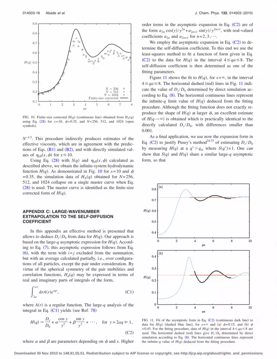
APPENDIX C: LARGE-WAVENUMBEREXTRAPOLATION TO THE SELF-DIFFUSIONCOEFFICIENT

In this appendix an effective method is presented thatallows to deduce Ds /D0 from data for H�q�. Our approach isbased on the large-q asymptotic expression for H�q�. Accord-ing to Eq. �7�, this asymptotic expression follows from Eq.�6�, with the term with i= j excluded from the summation,but with an average calculated partially, i.e., over configura-tions of all particles, except the pair under consideration. Byvirtue of the spherical symmetry of the pair mobilities andcorrelation functions, Hd�q� may be expressed in terms ofreal and imaginary parts of integrals of the form,

�2a

+�

drA�r�eiqr, �C1�

where A�r� is a regular function. The large-q analysis of theintegral in Eq. �C1� yields �see Ref. 78�

H�q� �Ds

D0+ �

cos y

y2 + �sin y

y3 + ¯ , for y = 2aq 1,

�C2�

where � and � are parameters depending on � and x. Higher

order terms in the asymptotic expansion in Eq. �C2� are ofthe form a2n cos�y� /y2n+a2n+1 sin�y� /y2n+1, with real-valuedcoefficients a2n and a2n+1 for n=2,3 ,¯.

We employ the asymptotic expansion in Eq. �C2� to de-termine the self-diffusion coefficient. To this end we use theleast-squares method to fit a function of form given in Eq.�C2� to the data for H�q� in the interval 4 qa 8. Theself-diffusion coefficient is then determined as one of thefitting parameters.

Figure 11 shows the fit to H�q�, for x=�, in the interval4 qa 8. The horizontal dashed �red� lines in Fig. 11 indi-cate the value of Ds /D0 determined by direct simulation ac-cording to Eq. �8�. The horizontal continuous lines representthe infinite-q limit value of H�q� deduced from the fittingprocedure. Although the fitting function does not exactly re-produce the shape of H�q� at larger �, an excellent estimateof H�q→�� is obtained which is practically identical to thedirectly calculated Ds /D0, with differences smaller than0.001.

As a final application, we use now the expansion form inEq. �C2� to justify Pusey’s method24,75 of estimating Ds /D0

by measuring H�q� at a q��qm where S�q��=1. One canshow that S�q� and H�q� share a similar large-q asymptoticform, so that

Finite-size correctedN = 1024N = 512N = 256

qa

H(q)

876543210

0.9

0.8

0.7

0.6

0.5

0.4

0.3

0.2

0.1

FIG. 10. Finite-size corrected H�q� �continuous line� obtained from HN�q�using Eq. �28� for x=10, �=0.35, and N=256, 512, and 1024 �opensymbols�.

(a)

qa

H(q)

1086420

0.8

0.7

0.6

0.5

0.4

(a)

qa

H(q)

1086420

0.8

0.7

0.6

0.5

0.4

(a)

qa

H(q)

1086420

0.8

0.7

0.6

0.5

0.4

(b)

qa

H(q)

1086420

0.4

0.3

0.2

0.1

0

(b)

qa

H(q)

1086420

0.4

0.3

0.2

0.1

0

(b)

qa

H(q)

1086420

0.4

0.3

0.2

0.1

0

FIG. 11. Fit of the asymptotic form in Eq. �C2� �continuous dark line� todata for H�q� �dashed blue line�, for x=� and �a� �=0.15, and �b� �=0.45. For the fitting procedure, data of H�q� in the interval 4 qa 8 areused. The horizontal dashed �red� lines give Ds /D0 determined by directsimulation according to Eq. �8�. The horizontal continuous lines representthe infinite-q value of H�q� deduced from the fitting procedure.



S�q� � 1 + ��cos y

y2 + ��sin y

y3 + ¯ , for y = 2aq 1.

�C3�

Equation �C3� differs from Eq. �C2� only in the expansioncoefficients, in particular in the infinite-q limit whereS�q→��=1. Thus, for a q��qm with S�q��=1, it followsfrom Eq. �C3� that H�q�� differs from Ds /D0 by terms oforder 1 / �aq��3 only.

1 T. Eckert and W. Richtering, J. Chem. Phys. 129, 124902 �2008�.2 E. Bartsch, V. Frentz, J. Baschnagel, W. Schärtl, and H. Sillescu, J.Chem. Phys. 106, 3743 �1997�.

3 S. Höfl, L. Zitzler, T. Hellweg, S. Herminghaus, and F. Mugele, Polymer48, 245 �2007�.

4 E. H. Purnomo, D. van den Ende, J. Mellema, and F. Mugele, Phys. Rev.E 76, 021404 �2007�.

5 E. H. Purnomo, D. van den Ende, S. A. Vanapalli, and F. Mugele, Phys.Rev. Lett. 101, 238301 �2008�.

6 C. A. Coutinho, R. K. Harrinauth, and V. K. Gupta, Colloids Surf., A318, 111 �2008�.

7 G. Petekidis, J. Gapinski, P. Seymour, J. S. van Duijneveldt, D. Vlasso-poulos, and G. Fytas, Phys. Rev. E 69, 042401 �2004�.

8 M. Zackrisson, A. Stradner, P. Schurtenberger, and J. Bergenholtz, Phys.Rev. E 73, 011408 �2006�.

9 M. Zackrisson, A. Stradner, P. Schurtenberger, and J. Bergenholtz, Lang-muir 21, 10835 �2005�.

10 P. A. Nommensen, M. H. G. Duits, J. S. Lopulissa, D. van den Ende, andJ. Mellema, Prog. Colloid Polym. Sci. 110, 144 �1998�.

11 P. A. Nommensen, M. H. G. Duits, D. van den Ende, and J. Mellema,Phys. Rev. E 59, 3147 �1999�.

12 P. A. Nommensen, M. H. G. Duits, D. van den Ende, and J. Mellema,Langmuir 16, 1902 �2000�.

13 H. M. Schaink, P. A. Nommensen, R. J. J. Jongschaap, and J. Mellema, J.Chem. Phys. 113, 2484 �2000�.

14 P. A. Nommensen, D. van den Ende, M. H. G. Duits, and J. Mellema,Langmuir 17, 5757 �2001�.

15 M. H. G. Duits, P. A. Nommensen, D. van den Ende, and J. Mellema,Colloids Surf., A 183–185, 335 �2001�.

16 P. Voudouris, J. Choi, H. Dong, M. R. Bockstaller, K. Matyjaszewski, andG. Fytas, Macromolecules 42, 2721 �2009�.

17 P. Debye and A. M. Bueche, J. Chem. Phys. 16, 573 �1948�.18 H.C. Brinkman, Appl. Sci. Res., Sect. A 1, 27 �1947�.19 P. Levresse, I. Manas-Zloczower, and D. L. Feke, Chem. Eng. Sci. 56,

3211 �2001�.20 L. Raynaud, B. Ernst, C. Verge, and J. Mewis, J. Colloid Interface Sci.

181, 11 �1996�.21 A. Weiss, N. Dingenouts, M. Ballauff, H. Senff, and W. Richtering, Lang-

muir 14, 5083 �1998�.22 A. J. C. Ladd, J. Chem. Phys. 93, 3484 �1990�.23 A. J. C. Ladd, H. Gang, J. X. Zhu, and D. A. Weitz, Phys. Rev. E 52,

6550 �1995�.24 P. N. Segrè, O. P. Behrend, and P. N. Pusey, Phys. Rev. E 52, 5070

�1995�.25 O. P. Behrend, Ph.D. thesis, University of Edinburgh, 1995.26 A. Sierou and J. F. Brady, J. Fluid Mech. 448, 115 �2001�.27 A. J. Banchio and J. F. Brady, J. Chem. Phys. 118, 10323 �2003�.28 J. F. Brady, Curr. Opin. Colloid Interface Sci. 1, 472 �1996�.29 A. J. Banchio, J. Gapinski, A. Patkowski, W. Häussler, A. Fluerasu, S.

Saccana, P. Holmqvist, G. Meier, M. P. Lettinga, and G. Nägele, Phys.Rev. Lett. 96, 138303 �2006�.

30 A. J. Banchio and G. Nägele, J. Chem. Phys. 128, 104903 �2008�.31 J. Gapinski, A. Patkowski, A. J. Banchio, J. Buitenhuis, P. Holmqvist, M.

P. Lettinga, G. Meier, and G. Nägele, J. Chem. Phys. 130, 084503�2009�.

32 W. B. Russel, D. A. Saville, and W. R. Schowalter, Colloidal Dispersions�Cambridge University Press, Cambridge, 1989�.

33 S. B. Chen, Phys. Fluids 10, 1550 �1998�.34 P. G. Wolynes and J. A. McCammon, Macromolecules 10, 86 �1977�.35 R. M. Wu, H. Y. Chung, and D. J. Lee, Chem. Eng. Sci. 59, 943 �2004�.36 S. B. Chen and A. Cai, J. Colloid Interface Sci. 217, 328 �1999�.37 G. Mo and A. S. Sangani, Phys. Fluids 6, 1637 �1994�.38 A. A. Potanin and W. B. Russel, Phys. Rev. E 52, 730 �1995�.39 S. L. Elliott and W. B. Russel, J. Rheol. 42, 361 �1998�.40 B. U. Felderhof, Physica A 151, 1 �1988�.41 B. Cichocki, B. U. Felderhof, K. Hinsen, E. Wajnryb, and J. Bławzdz-

iewicz, J. Chem. Phys. 100, 3780 �1994�.42 M. L. Ekiel-Jeżewska and E. Wajnryb, in Theoretical Methods for Micro

Scale Viscous Flows, edited by F. Feuillebois and A. Sellier �TransworldResearch Network, Kerala, 2009�.

43 R. Reuland, B. U. Felderhof, and R. B. Jones, Physica A 93, 465 �1978�.44 R. B. Jones and R. Schmitz, Physica A 149A, 373 �1988�.45 B. Cichocki, B. U. Felderhof, and R. Schmitz, PCH, PhysicoChem. Hy-

drodyn. 10, 383 �1988�.46 J. Bławzdziewicz, E. Wajnryb, and M. Loewenberg, J. Fluid Mech. 395,

29 �1999�.47 B. Cichocki and B. U. Felderhof, J. Chem. Phys. 130, 164712 �2009�.48 S. Kim and S. J. Karrila, Microhydrodynamics, �Dover, Mineola, 2005�.49 P. N. Pusey, in Liquids, Freezing and the Glass Transition, edited by J.-P.

Hansen, D. Levesque, and J. Zinn-Justin �Elsevier, Amsterdam, 1991�,pp. 763–942.

50 G. Nägele, Phys. Rep. 272, 215 �1996�.51 R. B. Jones and P. N. Pusey, Annu. Rev. Phys. Chem. 42, 137 �1991�.52 P. Szymczak and B. Cichocki, J. Stat. Mech.: Theory Exp. 2008, P0125

�2008�.53 G. Neale, N. Epstein, and W. Nader, Chem. Eng. Sci. 28, 1865 �1973�.54 B. U. Felderhof and R. B. Jones, Physica A 93, 457 �1978�.55 S. B. Chen and X. Ye, J. Colloid Interface Sci. 221, 50 �2000�.56 B. Cichocki, M. L. Ekiel-Jeżewska, and E. Wajnryb, J. Chem. Phys. 111,

3265 �1999�.57 B. Cichocki, M. L. Ekiel-Jeżewska, P. Szymczak, and E. Wajnryb, J.

Chem. Phys. 117, 1231 �2002�.58 R. G. Cox and H. Brenner, J. Fluid Mech. 28, 391 �1967�.59 P. Mazur and D. Bedeaux, Physica �Amsterdam� 76, 235 �1974�.60 B. U. Felderhof, Physica A 84, 569 �1976�.61 R. Schmitz and B. U. Felderhof, Physica A 113, 90 �1982�.62 R. Schmitz and B. U. Felderhof, Physica A 113, 103 �1982�.63 B. Cichocki, R. B. Jones, R. Kutteh, and E. Wajnryb, J. Chem. Phys. 112,

2548 �2000�.64 L. Durlofsky, J. F. Brady, and G. Bossis, J. Fluid Mech. 180, 21 �1987�.65 J. F. Brady and G. Bossis, Annu. Rev. Fluid Mech. 20, 111 �1988�.66 H. Hasimoto, J. Fluid Mech. 5, 317 �1959�.67 B. U. Felderhof, in Fundamental Problems in Statistical Mechanics VII,

edited by H. van Beijeren �North-Holland, Amsterdam, 1990�.68 G. H. Golub and C. F. Van Loan, Matrix Computations �The Johns Hop-

kins University Press, Baltimore, 1996�.69 G. C. Abade, Ph. D. thesis, University of Warsaw, Poland, 2009.70 L. Greengard and V. Rokhlin, J. Comput. Phys. 73, 325 �1987�.71 L. Verlet and J. J. Weis, Phys. Rev. A 5, 939 �1972�.72 W. R. Smith, D. J. Henderson, P. J. Leonard, J. A. Barker, and E. W.

Grundke, Mol. Phys. 106, 3 �2007�.73 G. K. Batchelor, J. Fluid Mech. 52, 245 �1972�.74 P. Szymczak and B. Cichocki, J. Chem. Phys. 121, 3329 �2004�.75 P. N. Pusey, J. Phys. A 11, 119 �1978�.76 D. O. Riese, G. H. Wegdam, W. L. Vos, R. Sprik, D. Fenistein, J. H. H.

Bongaerts, and G. Grübel, Phys. Rev. Lett. 85, 5460 �2000�.77 R. Schmitz and B. U. Felderhof, Physica A 92, 423 �1978�.78 A. Erdélyi, Asymptotic Expansions �Dover, New York, 1987�.



http://dx.doi.org/10.1063/1.2978383

http://dx.doi.org/10.1063/1.473464

http://dx.doi.org/10.1063/1.473464

http://dx.doi.org/10.1016/j.polymer.2006.10.026

http://dx.doi.org/10.1103/PhysRevE.76.021404


http://dx.doi.org/10.1103/PhysRevLett.101.238301


http://dx.doi.org/10.1016/j.colsurfa.2007.12.024




http://dx.doi.org/10.1021/la051664v

http://dx.doi.org/10.1021/la051664v

http://dx.doi.org/10.1007/BFb0118067


http://dx.doi.org/10.1021/la9906828

http://dx.doi.org/10.1063/1.482066

http://dx.doi.org/10.1063/1.482066

http://dx.doi.org/10.1021/la000972k

http://dx.doi.org/10.1016/S0927-7757(01)00527-1

http://dx.doi.org/10.1021/ma802878r

http://dx.doi.org/10.1063/1.1746948

http://dx.doi.org/10.1007/BF02120318

http://dx.doi.org/10.1016/S0009-2509(00)00542-X

http://dx.doi.org/10.1006/jcis.1996.0351

http://dx.doi.org/10.1021/la980356c

http://dx.doi.org/10.1021/la980356c

http://dx.doi.org/10.1063/1.458830



http://dx.doi.org/10.1017/S0022112001005912

http://dx.doi.org/10.1063/1.1571819



http://dx.doi.org/10.1063/1.2868773

http://dx.doi.org/10.1063/1.3078408

http://dx.doi.org/10.1063/1.869676

http://dx.doi.org/10.1021/ma60055a017

http://dx.doi.org/10.1016/j.ces.2003.12.014


http://dx.doi.org/10.1063/1.868227


http://dx.doi.org/10.1122/1.550940

http://dx.doi.org/10.1016/0378-4371(88)90036-2

http://dx.doi.org/10.1063/1.466366

http://dx.doi.org/10.1016/0378-4371(78)90167-X

http://dx.doi.org/10.1016/0378-4371(88)90111-2

http://dx.doi.org/10.1017/S002211209900590X

http://dx.doi.org/10.1063/1.3125382

http://dx.doi.org/10.1016/0370-1573(95)00078-X

http://dx.doi.org/10.1146/annurev.pc.42.100191.001033

http://dx.doi.org/10.1088/1742-5468/2008/01/P01025

http://dx.doi.org/10.1016/0009-2509(73)85070-5


http://dx.doi.org/10.1063/1.479605

http://dx.doi.org/10.1063/1.1484380

http://dx.doi.org/10.1063/1.1484380

http://dx.doi.org/10.1017/S0022112067002150

http://dx.doi.org/10.1016/0031-8914(74)90197-9

http://dx.doi.org/10.1016/0378-4371(76)90105-9

http://dx.doi.org/10.1016/0378-4371(82)90007-3

http://dx.doi.org/10.1016/0378-4371(82)90008-5

http://dx.doi.org/10.1063/1.480894

http://dx.doi.org/10.1017/S002211208700171X

http://dx.doi.org/10.1146/annurev.fl.20.010188.000551

http://dx.doi.org/10.1017/S0022112059000222

http://dx.doi.org/10.1016/0021-9991(87)90140-9

http://dx.doi.org/10.1103/PhysRevA.5.939

http://dx.doi.org/10.1080/00268970701628423

http://dx.doi.org/10.1017/S0022112072001399

http://dx.doi.org/10.1063/1.1767994

http://dx.doi.org/10.1088/0305-4470/11/1/014


http://dx.doi.org/10.1016/0378-4371(78)90141-3

Documents

Short-time dynamics of permeable particles in concentrated suspensions