Pattern Recognition 39 (2006) 921–934www.elsevier.com/locate/patcog

Signatures versus histograms: Definitions, distances and algorithms

Francesc Serratosaa,∗, Alberto Sanfeliub

aUniversitat Rovira I Virgili, Dept. d’Enginyeria Informàtica i Matemàtiques, SpainbUniversitat Politècnica de Catalunya, Institut de Robòtica i Informàtica Industrial, Spain

Received 14 June 2005; received in revised form 1 December 2005; accepted 5 December 2005

Abstract

The aim of this paper is to present a new method to compare histograms. The main advantage is that there is an important time-complexityreduction with respect to the methods presented before. This reduction is statistically and analytically demonstrated in the paper.

The distances between histograms that we presented are defined on a structure called signature, which is a lossless representation ofhistograms. Moreover, the type of the elements of the sets that the histograms represent are ordinal, nominal and modulo.

We show that the computational cost of these distances is O(z′) for the ordinal and nominal types and O(z′2) for the modulo one, z′being the number of non-empty bins of the histograms. The computational cost of the algorithms presented in the literature depends on thenumber of bins of the histograms. In most of the applications, the obtained histograms are sparse; then considering only the non-emptybins drastically decreases the time consumption of the comparison.

The distances and algorithms presented in this paper are experimentally validated on the comparison of images obtained from publicdatabases and positioning of mobile robots through the recognition of indoor scenes (captured in a learning stage).� 2006 Pattern Recognition Society. Published by Elsevier Ltd. All rights reserved.

Keywords: Distance between histograms; Signature; Earth mover distance; Second-order random graphs

1. Introduction

A histogram of a set with respect to a measurement repre-sents the frequency of quantified values of that measurementamong the samples. Finding the distance or similarity be-tween histograms is an important issue in pattern classifica-tion or clustering and image retrieval. For this reason, a num-ber of measures of similarity between histograms have beenproposed and used in computer vision and pattern recogni-tion. Protein classification is one of the common histogramapplications [1]. Moreover, if the ordering of the elements inthe sample is unimportant, the histogram obtained from thisset is a lossless representation of it and can be reconstructedfrom its histogram. Then, we can compute the distance be-tween sets in an efficient way by computing the distancebetween their histograms.

∗ Corresponding author. Tel.: +34 977558507.E-mail addresses: francesc.serratosa@urv.net (F. Serratosa),

sanfeliu@iri.upc.es (A. Sanfeliu).

0031-3203/$30.00 � 2006 Pattern Recognition Society. Published by Elsevier Ltd. All rights reserved.doi:10.1016/j.patcog.2005.12.005

The probabilistic approaches use histograms based on thefact that the histogram of a measurement provides the basisfor an empirical estimate of the probability density func-tion [2]. Computing the distance between probability den-sity functions can be regarded the same as computing theBayes probability. This is equivalent to measuring the over-lap between probability density functions as the distance.The B-distance [3], proposed by Kailath, measures the dis-tance between populations. It is a value between 0 and 1 andprovides bounds on the Bayes misclassification probability.An approach closely related to the B-distance was proposedby Matusita [4]. Finally, Kullback generalised the conceptof probabilistic uncertainty or “entropy” and introduced theK-L-distance measure [2,5] that is, the minimum cross en-tropy.

Most of the distance measures presented in the literature(there is an interesting compilation in Ref. [6]) considerthe overlap or intersection between two histograms as afunction of the distance value but they do not take into ac-count the similarity on the non-overlapping parts of the two

922 F. Serratosa, A. Sanfeliu / Pattern Recognition 39 (2006) 921–934

histograms. For this reason, Rubner presented in Ref. [7] anew definition of the distance measure between histogramsthat overcomes this non-overlapping parts problem. It wascalled Earth Mover’s Distance and it is defined as the mini-mum amount of work that must be performed to transformone histogram into the other by moving distribution mass.They used the simplex algorithm [8] to compute the distancemeasure and the method presented in Ref. [9] to search agood initialisation. Latter, Cha presented in Ref. [6] threealgorithms to obtain the distance between one-dimensionalhistograms that use the Earth Mover’s Distance. These algo-rithms computed the distance between histograms when thetype of measurements where nominal, ordinal and moduloin O(z), O(z) and O(z2), respectively, z being the numberof levels or bins.

Often, for specific set measurements, only a small fractionof the bins in a histogram contain significant information,that is, most of the bins are empty. This is more frequentwhen the dimensions of the element domain increase. Inthat case, the methods that use histograms as fixed-sizedstructures obtain poor efficiency. For this reason, Rubner [7]presented the variable-size descriptions called signatures.In that representation, the empty bins were not explicitlyconsidered.

If the statistical properties of the data are known a priori,the similarity measures can be improved by the smoothingprojections as it was shown in Ref. [10]. Moreover, this pro-jection can be applicable for reduction of the dimensionalityof the data and also to represent sparse data in a more tightform in the projection subspace.

Given two histograms, it is often useful to define a quan-titative measure of their dissimilarity with the intent of ap-proximating perceptual dissimilarity as well as possible. Tothat aim, we consider that a good definition of a distancebetween histograms needs to take into consideration a dis-tance between the basic features of the elements of the set.That is, similar pairs of histograms defined from differentbasic features may obtain different distance value betweenhistograms. We call the distance between set elements theground distance.

In Ref. [11], they performed image retrieval based oncolour histograms. Because the distance measure betweencolours is computationally expensive, they presented a lowdimensional and easy to compute distance measure. Theyshow that this measure is a lower bound on the colour-histogram distance measure.

An exact histogram-matching algorithm was presented inRef. [12]. The aim of this algorithm was to study the influ-ence of various image characteristics on colour reproduc-tion by perturbing them in a known way. Furthermore, thisperturbation would be done in a way whereby a set of het-erogeneous images would be the starting point and this setwould be transformed so as to make their histogram thesame for all the images. The aim of the algorithm was notthe comparison of histograms but to arrive to a transforma-tion look up table and transform the target image according

to it. An algorithm was presented in Ref. [13] to computethe distance between histograms that used the intersectionfunction, L1 norm, L2 norm and X2 test. The main featureof this algorithm was that the input was a built histogram(obtained from the target image) and another image. Then,it was not necessary to build the histogram of the image ofthe database to compute the distance between histograms.

Finally, the applications of the references commented be-fore use the histograms as global information of images.Histograms can also be used in structural pattern recogni-tion. For instance, Serratosa defined the function-describedgraphs [14], which is a structure that represents a clusterof attributed graphs in which there is a probability den-sity function in each node of the structure described by ahistogram.

Thus, to compare clusters (that is, to compare function-described graphs), a distance between histograms is neededto compare each of their nodes. Later, the same authorsdefined the second-order random graphs [15]. This struc-ture represents also a cluster of Attributed Graphs butthere is much amount of information since there is a jointprobability in each node described by a two-dimensionalhistogram. The computational cost of comparing graphsis exponential with respect to the number of nodes in theworst case. There are some efficient algorithms that ob-tain sub-optimal distances in polynomial cost with respectto the number of nodes [16]. For this reason, it is impor-tant to reduce the time consumption in comparing theirnodes.

In this paper, we present the algorithms to compute thedistances between histograms that the computational costdepends only on the non-empty bins instead of the num-ber of bins as it is in the algorithms presented in Refs.[6,7]. The type of measurements were nominal, ordinal andmodulo and the computational costs were O(z′), O(z′) andO(z′2), respectively, z′ being the number of non-empty binsof the histograms. We show that these distances obtain thesame value as the distances between histograms presentedin Ref. [6] although the computational time for each com-parison decreases when the histograms have a large size orthey are sparse. Furthermore, we suppose that we do nothave a priori probabilistic information of the histograms.For this reason, the methods presented in Ref. [10] are notuseful.

The subsequent sections are constructed as follows. First,we define the histograms and signatures. Then in Section 3we present three possible types of measurements and theirrelated distances. These distances will be used in the nextsection to define the distances between signatures. In Section5, we depict the basic algorithms to compute the distancesbetween signatures. In Section 6 we validate our algorithmson two different scenarios. The histograms to be comparedare obtained from images obtained from databases and in-door scenes, respectively. Finally, we conclude with empha-sis of the advantage of using the distance between signaturesand using the proposed algorithms.

F. Serratosa, A. Sanfeliu / Pattern Recognition 39 (2006) 921–934 923

2. Histograms and signatures

In this section, we formally give a definition of histogramsand signatures. The section finishes with a simple exampleto show the representations of the histograms and signaturesgiven a set of measurements.

2.1. Histogram definition

Let x be a measurement which can have one of T valuescontained in the set X = {x1, . . . , xT }. Consider a set of n

elements whose measurements of the value of x are A ={a1, . . . , an} where at ∈ X.

The histogram of the set A along the measurement x isH(x, A) which is an ordered list consisting of the numberof occurrences of the discrete values of x among the at .As we are interested only in comparing the histograms andsets of the same measurement x, H(A) will be used insteadof H(x, A) without loss of generality. If Hi(A), 1� i�T ,denotes the number of elements of A that have value xi , thenH(A) = [H1(A), . . . , HT (A)] where

Hi(A) =n∑

t=1

CAi,t (1)

H(A)

012345678

1 2 3 4 5 6 7 8 1 2 3 4 5 6 7 8

H(B)

012345678

Fig. 1. Sets A and B and their histograms.

mA

012345678

1 2 3 4012345678

1 2 3

W1A = 1

W2A = 4

W3A = 5

W4A = 6

mB

W1B = 1

W2B = 5

W3B = 8

Fig. 2. Signature representation of the sets A and B.

mA′

012345678

1 2 3 4 5

W1A′ = W1

B′ = 1W2

A′= W2B′= 4

W3A′= W3

B′= 5 W4

A′= W4B′= 6

W5A′= W5

B′= 8

mB′

012345678

1 2 3 4 5

Fig. 3. Extended signatures A′ and B ′. The number of elements mi are represented graphically and the value of its elements is represented by wi .

and the individual costs are defined as

CAi,t =

{1 if at = xi,

0 otherwise.(2)

The elements Hi(A) are usually called bins of the histogram.

2.2. Signature definition

Let H(A)=[H1(A), . . . , HT (A)] and S(A)=[S1(A), . . . ,

Sz(A)] be the histogram and the signature of the set A,respectively. Each Sk(A), 1�k�z�T , is composed of apair of terms, Sk(A) = {wk, mk}. The first term, wk , showsthe relation between the signature S(A) and the histogramH(A). Thus, if wk=i then the second term, mk , is the numberof elements of A that have value xi , that is, mk = Hi(A)

where wk < wt ⇔ k < t and mk > 0.The signature of a set is a lossless representation of its

histogram in which the bins of the histogram that have value0 are not expressed implicitly. From the signature definition,we obtain the following expression:

Hwk(A) = mk where 1�k�z. (3)

924 F. Serratosa, A. Sanfeliu / Pattern Recognition 39 (2006) 921–934

2.3. Extended signature

The extended signature is a signature in which the mini-mum number of empty bins has been added to assure that,given a pair of signatures to be compared, the number ofbins is the same. Moreover, each bin in both signatures rep-resents the same bin in the histograms.

2.4. Example

In this section we show a pair of sets with their histogramand signature representations. This example is used to ex-plain the distance measures in the next sections. Fig. 1 showsthe sets A and B and their histogram representations. Bothsets have 10 elements and values are contained from 1 to 8.The horizontal axis in the histograms represents the valuesof the elements and the vertical axis represents the numberof elements that have this value, that is, mi . Empty bins arethe ones that have mi = 0.

Fig. 2 shows the signature representation of the sets A andB. The length of the signatures is 4 and 3, respectively. Thevertical axis represents the number of elements of each binand the horizontal axis represents the bins of the signature.The set A has two elements with value 6 since this valueis represented by the bin 4 (WA

4 = 6) and the value of thevertical axis is 2 at bin 4. In the signature representationthere is no empty bin.

Fig. 3 shows the extended signatures of the sets A and B

with five bins. Note that the value that the extended signa-tures represents for each bin, wi , is the same for both signa-tures. Moreover, in A′ and B ′, one and two empty bins havebeen added, respectively.

3. Type of measurements and distance between them

We consider three types of measurements called nomi-nal, ordinal and modulo. In a nominal measurement, eachvalue of the measurement is a name and there is no relationbetween them such as greater than or lesser than (e.g. thenames of the students). In an ordinal measurement, the val-ues are ordered (e.g. the age of the students). Finally, in themodulo measurement, measurement values are ordered butform a ring due to the arithmetic modulo operation (e.g. theangle in a circumference). Corresponding to the three typesof measurements mentioned before, we define three mea-sures of difference between two measurement levels a ∈ X

and b ∈ X as follows:(a) Nominal distance:

dnom(a, b) ={

0 if a = b,

1 otherwise.(4)

The distance value between two nominal measurement val-ues is either match or mismatch, which is mathematicallyrepresented by 0 or 1.

(b) Ordinal distance:

dord(a, b) = |a − b|. (5)

The distance value between two ordinal measurement valuesis computed by the absolute difference of each element.

(c) Modulo distance:

dmod(a, b) ={ |a − b| if |a − b|�T/2,

T − |a − b| otherwise.(6)

The distance value between two modulo measurement valuesis the interior difference of each element.

Metric property: The three measures in Eqs. (4)–(6)satisfy the following necessary properties of a metric:

(a) Reflexivity: d(a, b) = 0.(b) Non-negativity: d(a, b)�0.(c) Commutativity: d(a, b) = d(b, a).(d) Triangle inequality: d(a, c)�d(a, b) + d(b, c).

Proof. Since they are straightforward facts, we omit theproofs. Moreover, the proof of the triangle inequality for themodulo distance is depicted in Ref. [6]. �

4. Distance between signatures

The aim of this section is to present the new distancesbetween signatures. To do so and for each type of element(nominal, ordinal and modulo), we first show the definitionof the distance between histograms and then we move on tothe new definitions of the distance between signatures. Thealgorithms used to obtain the extended signatures and thethree distances are described in Section 5.

For the following definitions of the distances and alsofor Section 5, we assume that the extended signatures ofS(A) and S(B) are S(A′) and S(B ′), respectively, whereSi(A

′) = {wA′i , mA′

i } and Si(B′) = {wB ′

i , mB ′i }. The number

of bins of S(A) and S(B) is zA and zB and the number ofbins of both extended signatures is z′.

4.1. Nominal distance

The nominal distance between histograms presented inRef. [6] is the number of elements that do not overlap orintersect. It is defined as follows:

Dnom(H(A), H(B)) =z∑

i=1

|Hi(A) − Hi(B)|. (7)

We define this distance through their extended signatures asfollows:

Dnom(S(A), S(B)) =z′∑

i=1

|mA′i − mB ′

i |. (8)

F. Serratosa, A. Sanfeliu / Pattern Recognition 39 (2006) 921–934 925

Theorem 1. The nominal-distance value between signa-tures is the same as the nominal-distance value between his-tograms.

Proof of Theorem 1. The bins in the histograms that arenot represented explicitly in the signatures are the ones thatin both histograms are empty, Hi(A)=Hi(B)=0. Then, theaddition of this bins does not affect the distance value. �

Example. We consider the extended signatures A′ and B ′shown in Fig. 3. The nominal distance is defined as theaddition of the difference between the number of elements.In this case it is 2 + 2 + 4 + 2 + 2 = 12.

4.2. Ordinal distance

The ordinal distance between two histograms was pre-sented in Ref. [7] as the minimum of work needed to trans-form one histogram to the other. Histogram H(A) can betransformed into histogram H(B) by moving the elementsto left or right and the total of all necessary minimum move-ments is the distance between them. There are two opera-tions. Suppose an element a belongs to the bin i. One oper-ation is move left (a). The result of this operation is that theelement a belongs to the bin i −1 and the cost to do so is 1.This operation is impossible for the elements that belong tothe bin 1. Another operation is move right (a). Similarly, af-ter the operation, a belongs to the bin i +1 and the cost is 1.The same restriction applies to the right most bin. These op-erations are graphically represented by right-to-left arrowsand left-to-right arrows. Fig. 4 shows the arrows needed totransform (a) histogram H(A) to histogram H(B) and (b)the extended signature S(A′) to S(B ′). The total number ofarrows is the distance value. It is the shortest movement andthere is no other way to move elements in shorter steps andtransform one histogram to the other. The distance betweenhistograms was defined in Ref. [6] as follows:

Dord(H(A), H(B)) =T −1∑i=1

∣∣∣∣∣∣i∑

j=1

(Hj (A) − Hj(B))

∣∣∣∣∣∣ . (9)

1 2 3 4 5 6 7 8

Dord(H(A),H(B)) Dord(S(A′),S(B′))

1 2 3 4 5

X3 X1 X1 X2

(a) (b)

Fig. 4. Arrow representation of the ordinal distance using (a) histogramsand (b) signatures.

There is a slight difference between Eq. (9) and the equationof the distance presented in Ref. [6]. They calculated thecase i = T , which we have not considered in Eq. (9) sincethe addition of all the arrows is always 0 when the sets havethe same number of elements.

We have defined our new distance between signaturessimilarly to the distance between histograms as follows:

Dord(S(A), S(B))

=z′−1∑i=1

⎡⎣(wA′

i+1 − wA′i )

∣∣∣∣∣∣i∑

j=1

(mA′j − mB ′

j )

∣∣∣∣∣∣⎤⎦ . (10)

The main difference is that we have to take into considerationthat the difference between bins is not constant. In Eq. (9),the number of arrows that goes from bin i to bin i + 1 is

described by∣∣∣∑i

j=1(Hj (A) − Hj(B))

∣∣∣ and the cost of one

arrow (or the operation move right or move left) is 1 asdescribed before. Our arrows do not have a constant size (orconstant cost) but they depend on the distance between bins.If element a belongs to the bin i, the operation move left (a)results in the element a belonging to bin i − 1 and the costfor doing so being wi − wi−1. Similarly, after the operationmove right (a), the element a belongs to the bin i+1 and thecost is wi+1−wi . In Eq. (10), the number of arrows that goes

from bin i to bin i + 1 is described by∣∣∣∑i

j=1(mA′j − mB ′

j )

∣∣∣and the cost of these arrows is wi+1 − wi .

In the extreme case in which the signature and the his-togram have equal number of bins, all the arrows have length1 due to wi − wi−1 = 1 and we obtain similar expressionsin both distances.

Example. Fig. 4 shows the graphic representation of thearrows in the histogram distance (a) and in the signaturedistance (b). They represent the minimum necessary move-ments. In the case of the distance between histograms, thedistance is the number of arrows. But in the signature case,the distance is the number of arrows multiplied by the lengthof the arrows (shown under the arrows). For instance, in thefirst arrows, the length is 3 since wA′

1 − wA2 = 4 − 1 = 3.

The distance value between signatures is 3 × 2 + 1 × 4 +2 × 2 = 14, which is the number of arrows in the histogramdistance.

Theorem 2. The ordinal-distance value between signa-tures is the same as the ordinal-distance value betweenhistograms.

The following lemma makes easier the demonstration ofthe theorem. First, suppose that the relation between the binsof the extended signatures and histograms is wk = i andwk+1 = p, p > i.

Lemma 1. The accumulative addition of the difference be-tween histograms is the same as the accumulative addition

926 F. Serratosa, A. Sanfeliu / Pattern Recognition 39 (2006) 921–934

of the difference between extended signatures when wk = i.

i∑j=1

(Hj (A) − Hj(B)) =k∑

j=1

(mA′j − mB ′

j ). (11)

Proof of Lemma 1. This is a straightforward fact since theterms that Hj(A) = Hj(B) = 0 are not considered in theextended signatures and also Hj(A) − Hj(B) = 0. �

Proof of Theorem 2. By definition of the extended signa-tures we have

Hi(A) �= 0 or Hi(B) �= 0Hi+1(A) = 0 and Hi+1(B) = 0...

Hp−1(A) = 0 and Hp−1(B) = 0

⎫⎬⎭

Hp(A) �= 0 or Hp(B) �= 0

(p − i − 1)

≡ (wk+1 − wk − 1) files. (12)

Then, it is easy to see that∑i

j=1(Hj (A) − Hj(B)) =∑pj=1(Hj (A)−Hj(B)). So, if we add the absolute value of

these terms as∑p

t=i |∑t

j=1(Hj (A) − Hj(B))|, we get that

this expression is similar to (p−i)|∑ij=1(Hj (A)−Hj(B))|.

If we substitute (p − i) by (wk+1 − wk) and we useEq. (11) we arrive at the following expression:

p∑t=i

∣∣∣∣∣∣t∑

j=1

(Hj (A) − Hj(B))

∣∣∣∣∣∣= (wA′

k+1 − wA′k )

∣∣∣∣∣∣k∑

j=1

(mA′j − mB ′

j )

∣∣∣∣∣∣ .

This expression is true for all the bins, so we obtain Eq. (10)by adding all the terms. �

4.3. Modulo distance

One major difference in a modulo type histogram or sig-nature is that the first bin and the last bin are consideredto be adjacent to each other, and hence, it forms a closedcircle, due to the nature of the data type. Transforming amodulo type histogram or signature to another while com-puting their distance should allow cells to move from thefirst bin to the last one or vice versa at a cost of a singlemovement. Now, cells or blocks of earth can move from thefirst bin to the last bin with the operation move left (1) inthe histogram case or move left (w1) in the signature case.Similarly, blocks can move from the last bin to the first onewith the operations move right (T ) in the histogram case ormove right (wz′ ) in the signature case.

The cost of these operations is calculated similarly as thecost of the operations in the ordinal distance except for themovements of blocks from the first bin to the last one orvice versa. In the case of the distance between histograms,the cost is one, as in all the movements. In the case of the

0

1

2

3

4

5

6

7

8

1 2 3 4 5 6 7 8

(a) (b)(b) (c)

Wz′ T1 W1

Fig. 5. The three terms that have to be considered to compute the costof moving blocks from the last bin to the first one or vice versa in themodulo distance between signatures.

Dmod(H(A),H(B))

1 2 3 4 5 6 7 8

Dmod(S(A′),S(B′))

1 2 3 4 5

X1 X1 X1

(a) (b)

Fig. 6. Arrow representation of the modulo distance using (a) histogramsand (b) signatures.

distance between signatures, it has to be considered as thereal distance between bins or the length of the arrows. Thus,the cost of these movements is the addition of three terms(see Fig. 5): (a) the cost from the last bin of the signature,wz′ , to the last bin of the histogram, T ; (b) the cost from thelast bin of the histogram, T , to the first bin of the histogram,1; (c) the cost from the first bin of the histogram, 1, to thefirst bin of the signature, w1. Then, the costs are calculatedas the length of these terms. The cost of (a) is T − wz′ , thecost of (b) is 1 (similarly to the cost between histograms)and the cost of (c) is w1 − 1. Therefore, the final cost fromthe last bin to the first one or vice versa between signaturesis w1−wz′ + T .

Example. Fig. 6 shows graphically the minimum arrowsnecessary to get the modulo distance in (a) the histogramcase and (b) the signature case. The distance is obtained sim-ilarly as in the ordinal example except that arrows from thefirst bin to the last one are allowed or vice versa. The valueof the distance between signatures is 2×1+2×1+2×1=6.In this signature representation, the cost of the two arrowsthat go from the first bin to the last bin is 1. This is due tothe fact that w1 = 1 (first bin in the histogram representa-tion) and w5 = 8 (last bin in the histogram representation,T = 8). Then this cost is 1 − 8 − 8 = 1.

Due to the modulo properties explained before, we cantransform one signature or histogram into another in several

F. Serratosa, A. Sanfeliu / Pattern Recognition 39 (2006) 921–934 927

X3 X1 X1 X2

1 2 3 4 5 1 2 3 4 5 1 2 3 4 5

X1 X3 X1 X1 X2 X1 X3 X1 X1 X2

(a) (b) (c)

Fig. 7. (a) Arrow representation of the modulo distance between signatures.(b) Addition of a chain of left arrows. (c) The final arrow representation.

ways. Among these ways, there exists a minimum distancewhose number of movements (or the cost of the arrows andthe number of arrows) is the lowest. If there is a borderline between bins that have both directional arrows, theyare cancelled out. These movements are redundant and sothe distance cannot be obtained through this configurationof arrows. To find the minimum configuration of arrows,we can add a complete chain in the histogram or signatureof same directional arrows, then the opposite arrows on thesame border between bins are cancelled out. Fig. 7 showsthe operation of adding a chain of left arrows to an arrowrepresentation. The cost of the first representation is 3 ×2 + 1 × 4 + 1 × 0 + 2 × 2 = 14 and the cost of the lastrepresentation is 1 × 1 + 3 × 1 + 1 × 3 + 1 × 1 + 2 × 1 = 10.

An algorithm to compute the modulo distance betweenhistograms was presented in Ref. [6] although the mathe-matical expression of the distance was not described. Wepropose here a new expression for the modulo distance thattheir algorithm calculates

Dmod(H(A), H(B)) = minc

⎧⎨⎩

T −1∑i=1

⎡⎣

∣∣∣∣∣∣c +i∑

j=1

(Hj (A)

−Hj(B))

∣∣∣∣∣∣⎤⎦ + |c|

⎫⎬⎭ , (13)

where c represents the chains of left arrows or right arrowsadded to the current arrow representation. The absolute valueof c at the end of the expression is the number of chains

1 2 3 4 5

X1 X3 X1 X1 X2

1 2 3 4 5

X3 X1 X1 X2

1 2 3 4 5

X1 X3 X1 X1 X2

1 2 3 4 5

X1 X3 X1 X1 X2

1 2 3 4 5

X1 X3 X1 X1 X2

c=1 c=0 c=-1 c=-2 c=-3 cost=22 cost=14 cost=10 cost=6 cost=12

Fig. 8. Five different transformations of signature S(A) to signature S(B) with their related c and the obtained cost.

added to the current representation. It comes from the costof the arrows from the last bin to the first one or vice versa.

The modulo distance between signatures is defined simi-larly as follows:

Dmod(S(A), S(B))

= minc

⎧⎨⎩

z′−1∑i=1

⎡⎣(wA′

i+1 − wA′i )

∣∣∣∣∣∣c +i∑

j=1

(mA′j − mB ′

j )

∣∣∣∣∣∣⎤⎦

+ (wA′1 − wA′

z′ + T )|c|⎫⎬⎭ . (14)

This expression is similar to the one for the histograms. Themain difference is that the cost of moving a block of earthfrom one bin to another one is not 1 but it is the length of thearrows or the distance between the bins (as it was explainedin the ordinal distance between signatures). The cost of themovement of blocks from the first bin to the last one or viceversa is w1 −wz′ + T and the costs of the other movementsare wA′

i+1 − wA′i .

Example. Fig. 8 shows five different transformations of sig-nature S(A) to signature S(B) and their related costs. Inthe first transformation, one chain of right arrows are added(c = 1). In the second one, no chains are added (c = 0),thus the cost is the same as the ordinal distance. In the thirdto the last ones, 1, 2 and 3 chains of left arrows are added,respectively. We can see that the minimum cost is 6 and itis the case that c = −2; then the distance value is 6 for themodulo distance and 14 for the ordinal distance.

Theorem 3. The ordinal-distance value between signa-tures is the same as the ordinal-distance value betweenhistograms.

Proof of Theorem 3. The proof that both distances are thesame is very similar to the one for the ordinal distance.We assume the situation of Eq. (12); then, we have thatc +∑i

j=1(Hj (A)−Hj(B))= c +∑pj=1(Hj (A)−Hj(B)).

So, if we add the absolute value of these terms as∑p

t=i |c +∑tj=1(Hj (A) − Hj(B))|, we get that this expression is

928 F. Serratosa, A. Sanfeliu / Pattern Recognition 39 (2006) 921–934

similar to (p− i)|c+∑ij=1(Hj (A)−Hj(B))|. If we substi-

tute (p − i) by (wk+1 − wk) and we use Eq. (11) we arriveat the following expression:

p∑t=i

∣∣∣∣∣∣c +t∑

j=1

(Hj (A) − Hj(B))

∣∣∣∣∣∣= (wA′

k+1 − wA′k )

∣∣∣∣∣∣c +k∑

j=1

(mA′j − mB ′

j )

∣∣∣∣∣∣ .

This expression is true for all the bins, so we obtain Eq. (14)by adding all the terms. �

5. Algorithms

We present the pseudo-code of four algorithms. The firstone extends two signatures, which is the first step to com-pute the distances between signatures. The other algorithmscompute the distance between signatures.

5.1. Extended signatures

Given two signatures, the process Extended_Signature ob-tains two minimum extended signatures and the number ofbins of both extended signatures. The two extended signa-tures have the same number of bins but each one has thesame information as the original signature. To do so, somebins with null value have to be added.

{S(A′),S(B ′), z′}=Extended_Signature {S(A),S(B)}1. i = 0 j = 0 z′ = 02. while(i < zA or j < zB)

3. if(wAi < wB

j or j = zB)

4. wA′z′ = wB ′

z′ = wAi

5. mA′z′ = mA

i mB ′z′ = 0

6. i++ z′++7. else if(wA

i > wBj or i = zA)

8. wA′z′ = wB ′

z′ = wBj

9. mA′z′ = 0 mB ′

z′ = mBj

10. j++ z′++11. else //wA

i = wBj and i < zA and j < zB

12. wA′z′ = wB ′

z′ = wAi

13. mA′z′ = mA

i mB ′z′ = mB

j

14. i++ j++ z′++

Correctness of the procedure:The aim of the algorithm is to fill the extended signatures

with the values of both signatures taking into considerationthe order of the positions of the bins. We can discern threedifferent cases. In the first one (lines 3–6), the extendedsignature A′ is filled with information and B ′ with an emptybin. This is because the order of the bin in the signatureA is smaller than the one in B or because there are no

more bins in B. In the second one (lines 7–10), we havethe inverse situation. And in the last case (lines 11–14),both bins in the signatures are non-empty and so their ex-tended signatures are filled with the same value. The worst-case time complexity of this procedure is O(z), z being thelength of both histograms. This is the case when the inter-section of the signatures is null and the union of them has nonon-empty bins. Then, the execution of the procedure nevergoes through lines 11–14 and the extended signatures havez bins. The best-case time complexity appears when bothsignatures and also the union of them have the same numberof bins.

5.2. Nominal distance

The process Nominal_Distance obtains the value of thenominal distance of two signatures.

Dnom= Nominal_Distance {S(A), S(B)}{S(A′),S(B ′),z′}=Extended_Signature {S(A), S(B)}1.Dnom = 02. for (i = 1 to z′)3. Dnom + =abs(mA′

i − mB ′i )

Correctness of the procedure:Since it is a straightforward fact, we omit the proof. The

time complexity of this procedure is O(z′), z′ being thenumber of bins of the extended signatures. The worst caseappears when the length of the extended signatures is thelength of the histograms, z′ = z.

5.3. Ordinal distance

The process Ordinal_Distance obtains the value of theordinal distance of two signatures.

Dord= Ordinal_Distance {S(A),S(B)}{S(A′),S(B ′),z′}=Extended_Signature {S(A),S(B)}1.Dord = 0 p = 02. for (i = 1 to z′ − 1)

3. p + =mA′i − mB ′

i

4. Dnom + =(wA′i+1 − wA′

i ) ∗ abs(p)

The algorithm computes, for each bin, the sum of theproduct of two terms. The first one is the length of each arrow(distance between the ith bin and the i + 1th), representedby (wA′

i+1 −wA′i ) and the second one is the number of arrows

between the bins, represented by the absolute value of p.Correctness of the procedure: The following lemma is

crucial for the demonstration of the correctness of the algo-rithm. First, suppose that we have successfully constructedthe arrow representation of the histograms such that the dis-tance is the minimum.

Lemma 2. Let the variable of the algorithm p at step i de-note the number of arrows from the bin i to the bin i + 1

F. Serratosa, A. Sanfeliu / Pattern Recognition 39 (2006) 921–934 929

of the extended signatures. It is positive if arrows are head-ing to right or negative otherwise. The algorithm computesp as follows:

p =i∑

j=1

(mA′i − mB ′

i ). (15)

Proof of Lemma 2. Consider two extended sub-signatures,S1,...,i (A

′) and S1,...,i (B′), where bins are 1 to i. After trans-

forming, population of S1,...,i (A′) + p must be equal to that

of S1,...,i (B′). If p �= ∑i

j=1mA′i − ∑i

j=1mB ′i then there is

no way to transform S1,...,i (A′) to S1,...,i (B

′) + p. By con-tradiction, Eq. (15) holds. �

Theorem 4. The procedure Ordinal_Distance correctlyfinds the minimum distance between two signatures.

Proof of Theorem 4. Note that, given a pair of signatures,the distribution of the arrows is the only variable of thedistance since the length of the arrows is a constant. As Eq.(15) is true for all levels and it is the only way to trans-form one sub-signature to another one, the distance has tobe obtained as this distribution of arrows. Therefore, the dis-tance is obtained by

∑ij=1[(mA′

i − mB ′i )|p|]. This is equiv-

alent to the equation of distance (14) if p is substitutedusing Eq. (15).

The time complexity of this procedure is O(z′) as in thenominal case. �

5.4. Modulo distance

The process Modulo_Distance obtains the modulo dis-tance of two signatures.

Dmod= Modulo_Distance {S(A), S(B)}{S(A′), S(B ′), z′}= Extended_Signature {S(A), S(B)}1. Dmod = 0 p[0] = mA′

0 − mB ′0

2. for (i = 2 to z′) p[i] = mA′i − mB ′

i + p[i − 1]3. for (i = 1 to z − 1′) Dmod + =(wA′

i+1 − wA′i ) ∗ abs(p[i])

4. do5. D2 = 06. c= min positive {p[i] for 1� i�z′}7. T emp[i] = p[i] − c for 1� i�z′8. for (i = 1 to z′ − 1) D2 + =(wA′

i+1 − wA′i ) ∗ abs(T emp[i])

9. if (Dmod > D2) Dmod = D210. p[i] = T emp[i] for 1� i�z′11. while(Dmod > D2)

12. do13. D2 = 014. c= maxnegative {p[i] for 1� i�z′}15. T emp[i] = p[i] − c for 1� i�z′16. for (i = 1 to z′ − 1) D2 + =(wA′

i+1 − wA′i ) ∗ abs(T emp[i])

17. if (Dmod > D2) Dmod = D218. p[i] = T emp[i] for 1� i�z′19. while(Dmod > D2)

Correctness of the procedure:The arrow representation of minimum distance can be

achieved from any arbitrary valid arrow representation bycombination of two basic operations: increasing the chainsof right arrows (when the value of c is positive) or increasingthe chains of left arrows (when the value of c is negative).The distance value can increase infinitely but there existsonly one minima among valid representations. In order toreach to the minima, first the algorithms test for increasingpositively c whether it gives higher or lower distance value.If the distance reduces, keep applying the operations until nomore reduction occurs. Then, the algorithms does the sameoperation but increasing negatively c. With these two actions,the algorithm guarantees that all possible combinations ofcorrect representations of arrows are tested.

The procedure runs in O(z′2) time. Lines 1–3 obtainthe ordinal distance. In lines 4–11 chains of right arrowsare added to the current arrow representation until there isno more reduction to the total number of arrows. This in-crement is considered in the algorithm by the variable c.Next, chains of left arrows are added in a similar manner(lines 12–19).

6. Validation of the method and algorithms

The method and algorithms presented in this paper areapplied on histograms, independently on the kind of theoriginal set from which they have been obtained, i.e. images[20], discretized probability-density functions [14]. The onlycondition to use our method is to know the type of elementsof the original set: ordinal, nominal or modulo.

In this paper, we validate our method on the comparisonof images. We use the distance between histograms as a

930 F. Serratosa, A. Sanfeliu / Pattern Recognition 39 (2006) 921–934

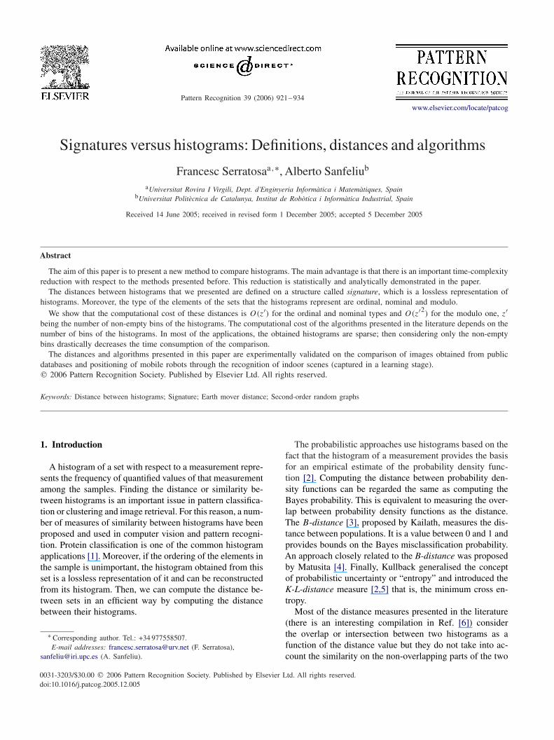
Table 1Illumination 28 bins

Length Increase Correct. Decreasespeed (%) correct.

Histo. 265 1 78 1Signa. 235 1.12 78 1Signa. 157 1.68 78 1100Signa. 106 2.50 69 0.88200Signa. 57 4.64 57 0.73300

Ordinal histogram.

metric to compare images. It is important to note that weare not interested in the sophisticated techniques of imageretrieval, i.e. Refs. [17–19]. We show that, using our algo-rithms, the classification of images through their histogramsis really fast and keeps a high ratio of correctness. Someimage retrieval techniques could be applied using our tech-nique as the distance between images.

In the next two sections, we first experiment on imagesobtained from databases and second on indoor scenes. Inboth experiments, we show that there is an important re-duction of the run time when the signature distance is usedwith respect to the histogram distance, although the ratio ofrecognition does not decrease.

6.1. Experiment with colour images

To show the validity of our new method, we have firsttested the ordinal and modulo distances between histogramsand between signatures. We used 1000 images (640 × 480pixels) obtained from public databases. To validate the or-dinal distance, we calculate the histograms from the illu-mination coordinate with 28 levels (Table 1) and with 216

levels (Table 3). And also, to test the modulo distance,the histograms represent the hue coordinate with 28 levels(Table 2) and with 216 levels (Table 4). Each of the tablesbelow shows the results of five different tests. In the first andsecond files of the tables, the distance were computed be-tween histograms and signatures, respectively. In the otherthree, the distance was computed between signatures but,with the aim of reducing the length of the signature (and soto increase the speed), the bins that had elements less than100, 200 or 300 in Tables 1 and 2 and elements less than1, 2 or 3 in Tables 3 and 4 were removed. The first columnis the number of bins of the histogram (first cell) or signa-tures (the other four cells). The second column representsthe increase of speed if we use signatures with respect tohistograms. It is calculated as the ratio between the run timeof the histogram method and the signature method. The thirdcolumn is the average correctness. The last column repre-sents the decrease of correctness due to the use of signa-tures with filtered histograms. It is obtained as the ratio of

Table 2Hue 28 bins

Length Increase Correct. Decreasespeed (%) correct.

Histo. 265 1 86 1Signa. 215 1.23 86 1Signa. 131 2.02 85 0.98100Signa. 95 2.78 73 0.84200Signa. 45 5.88 65 0.75300

Modulo histogram.

Table 3Illumination 216 bins

Length Increase Correct. Decreasespeed (%) correct.

Histo. 6,536 1 81 1Signa. 245 267.49 81 1Signa. 115 569.87 81 11Signa. 87 753.28 67 0.822Signa. 32 2048.00 55 0.673

Ordinal histogram.

Table 4Hue 216 bins

Length Increase Correct. Decreasespeed (%) correct.

Histo. 65,536 1 89 1Signa. 205 319.68 89 1Signa. 127 516.03 89 11Signa. 99 661.97 78 0.872Signa. 51 1285.01 69 0.773

Modulo histogram.

the correctness of the histogram to the correctness of eachfilter.

Tables 1–4 show us that our method is much useful whenthe number of levels increases since the number of emptybins tends to increase. Moreover, while comparing the his-togram of the hues, the increase is much important becausethe algorithm has a quadratic computational cost. Note thatin the case of the first filter (third experiment in the tables),there is no decrease in the correctness although there is muchincrease in the speed with respect to the signature method(second experiment).

F. Serratosa, A. Sanfeliu / Pattern Recognition 39 (2006) 921–934 931

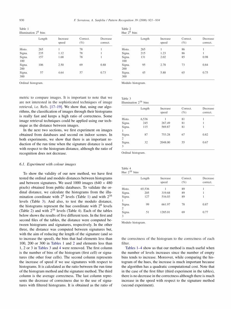
Fig. 9. Images from indoor scenes. Below each image, its luminance and hue histogram.

932 F. Serratosa, A. Sanfeliu / Pattern Recognition 39 (2006) 921–934

Fig. 9. (continued).

F. Serratosa, A. Sanfeliu / Pattern Recognition 39 (2006) 921–934 933

Table 5Mismatched images and ratio of recognition using luminance and huehistograms and the three distances: cardinal, ordinal and modulo

Histogram Distance Mismatched images Recognition (%)

Luminance Cardinal 1,3,8,12,16,17,18 70.8Luminance Ordinal 3,16,19 87.5Hue Modulo 15,17 91.6

6.2. Experiment on indoor scenes

Signatures have also been compared with histograms us-ing indoor scenes. These scenes were used for robot posi-tioning. In the learning stage, the robot is guided through theoffices and corridors while the exact position is introducedand the robot captures the scenes. In the recognition stage,the robot assumes to be in the position that captures the mostsimilar scene obtained in the learning stage. The main ad-vantage of this technique (also reported in Refs. [21,22]) isthat any mechanical method is not needed. Moreover, im-age retrieval techniques are not used, since the new sceneis not compared to all the scenes of the database, but onlyto the ones that are known to be near to the supposed po-sition of the robot. Finally, if the scene is not recognised,the last position of the robot is assumed to be the presentone and another image is captured. In Ref. [22], a samerobot-positioning method was used. The main difference isthat they used structural information of the image and theyneeded to segment the image. For this reason, the ratio ofrecognition was supposed to be higher, but also the com-putational time. The main advantage of our method is thatthe image is not to be processed, only the histogram of it isneeded.

Fig. 9 shows eight different scenes. From each scene, wehave taken three images with a slight difference of position.Furthermore, we show the histogram of the luminance andthe hue of these images. We have used the histograms ofthe luminance to test the cardinal and ordinal distance andthe other histograms to test the modulo distance. Note thatthere is a similarity between the three histograms of the samescene and also that the hue histograms are much sparse thanthe luminance ones.

Table 6Run time and ratio of recognition obtained from three experiments on the luminance histograms (a) and (b) and on the hue histograms (c)

Card. dist. Ord. dist. Mod. dist.

Histo. Sign. Histo. Sign. Histo. Sign.

No Filter Filter No Filter Filter No Filter Filterfilter a b filter a b filter a b

Run time 100 85 51 24 105 87 45 21 526 233 78 69% Recog. 70.8 70.8 70.5 55.3 87.5 87.5 87.3 75.2 91.6 91.6 91.4 87.2

Table 5 shows the mismatched images and the ratio ofrecognition using the cardinal and ordinal distances forthe luminance histogram and the modulo distance for thehue histogram. We consider a mismatched image if thethree images that obtained smaller distance are not from itsscene. As it is expected, the hue histograms obtain betterresults. Nevertheless, there is not a big difference, theseimages are not much saturated and so there is few informa-tion on the hue. This is the reason the hue histograms aresparse.

Table 6 shows the run time and ratio of recognitionobtained from three experiments. In the first one (a), theresults were computed using the cardinal distance on theluminance histograms. In the second one (b), the cardinaldistance was changed by the ordinal distance. And in thethird experiment (c), the modulo distance was computed onthe hue histograms. From each experiment, we obtained therun time and the ratio of recognition in four cases: (1) com-paring histograms, (2) comparing signatures, (3) comparingfiltered signatures. The threshold of the filter was situated asmuch higher as possible, when that the ratio of recognitionbegan to decrease. (4) The same as the third case but witha higher threshold of the filter. In all the cases, the run timewas normalised such that the run time of the histogram inthe first case was 100.

It is interesting to realise the decrease on the run timein the case of the modulo distance when a filter is applied.There is a decrease from 526 to 78.

7. Conclusions and future work

We have presented the nominal, ordinal and modulo dis-tance between signatures and the algorithms used to com-pute them. We have shown that signatures are a lossless rep-resentation of histograms and that computing the distancebetween signatures is the same as between histograms butwith a lower computational time. We have validated thesenew algorithms with a huge amount of real images andwe have realised that there is an important time saving be-cause most of the histograms are sparse. Moreover, if weapply filtering techniques on the histograms, the number ofbins of the signatures reduces and so the run time of theircomparison.

934 F. Serratosa, A. Sanfeliu / Pattern Recognition 39 (2006) 921–934

Although the signatures and histograms that we dealt within this paper are one-dimensional, it can be useful in manyapplications in the comparison between multi-dimensionalhistograms. The only difference in our equations of the dis-tances would be the definition of the ground distance (nom-inal, ordinal or modulo). Nevertheless, defining the algo-rithms to compute the distance between multi-dimensionalsignatures is non-trivial because of the increase of possibleassignments. We leave the design of fast algorithms to com-pute these distances as open problems.

References

[1] Y.-P. Nieh, K.Y.J. Zhang, A two-dimensional histogram-matchingmethod for protein phase refinement and extension, Biol. Crystallogr.55 (1999) 1893–1900.

[2] R.O. Duda, P.E. Hart, D.G. Stork, Pattern Classification, second ed.,Wiley, New York, 2000.

[3] T. Kailath, The divergence and Bhattacharyya distance measures insignal selection, IEEE Trans. Community Technol. COM-15 1 (1967)52–60.

[4] K. Matusita, Decision rules, based on the distance, for problems offit, two samples and estimation, Ann. Math. Stat. 26 (1955) 631–640.

[5] J.E. Shore, R.M. Gray, Minimum cross-entropy pattern classificationand cluster analysis, Trans. Pattern Anal. Mach. Intell. 4 (1) (1982)11–17.

[6] S.-H. Cha, S.N. Srihari, On measuring the distance betweenhistograms, Pattern Recognition 35 (2002) 1355–1370.

[7] Y. Rubner, C. Tomasi, L.J. Guibas, A metric for distributions withapplications to image databases, Int. J. Comput. Vision 40 (2) (2000)99–121.

[8] Numerical recipes in C: the art of scientific computing, ISBN 0-521-43108-5.

[9] E.J. Russell, Extension of Dantzig’s algorithm to finding an initialnear-optimal basis for the transportation problem, Oper. Res. 17(1969) 187–191.

[10] J.-K. Kamarainen, V. Kyrki, J. Llonen, H. Kälviäinen, Improvingsimilarity measures of histograms using smoothing projections,Pattern Recognition Lett. 24 (2003) 2009–2019.

[11] J. Hafner, J.S. Sawhney, W. Equitz, M. Flicker, W. Niblack, Efficientcolour histogram indexing for quadratic form distance functions,Trans. Pattern Anal. Mach. Intell. 17 (7) (1995) 729–735.

[12] J. Morovic, J. Shaw, P.-L. Sun, A fast, non-iterative and exacthistogram matching algorithm, Pattern Recognition Lett. 23 (2002)127–135.

[13] F.-D. Jou, K.-Ch. Fan, Y.-L. Chang, Efficient matching of large-sizehistograms, Pattern Recognition Lett. 25 (2004) 277–286.

[14] F. Serratosa, R. Alquézar, A. Sanfeliu, Function-described graphsfor modeling objects represented by attributed graphs, PatternRecognition 36 (3) (2003) 781–798.

[15] A. Sanfeliu, F. Serratosa, R. Alquézar, Second-order random graphsfor modeling sets of attributed graphs and their application to objectlearning and recognition, Int. J. Pattern Recognition Artif. Intell. 18(3) (2004) 375–396.

[16] F. Serratosa, R. Alquézar, A. Sanfeliu, Efficient algorithms formatching attributed graphs and function-described graphs, in:Proceedings of the 15th International Conference on PatternRecognition, ICPR’2000, Barcelona, Spain, 2000.

[17] W. Jiang, G. Er, Q. Dai, J. Gu, Hidden annotation for image retrievalwith long-term relevance feedback learning, Pattern Recognition 38(11) (2005) 2007–2021.

[18] K. Lu, X. He, Image retrieval based on incremental subspace learning,Pattern Recognition 38 (11) (2005) 2047–2054.

[19] Y. Peng-Yeng, B. Bhanu, Ch. Kuang-Cheng, A. Dong, Integratingrelevance feedback techniques for image retrieval using reinforcementlearning, Pattern Anal. Mach. Intell. 27 (10) (2005) 1536–1551.

[20] M. Pi, M.K. Mandal, A. Basu, Image retrieval based on histogramof fractal parameters, Multimedia, IEEE Trans. 7 (4) (2005)597–605.

[21] G. Wells, Ch. Venaille, C. Torras, Vision-based robot positioningusing neural networks, Image Vision Comput. 14 (10) (1996)715–732.

[22] E. Staffeti, A. Grau, F. Serratosa, A. Sanfeliu, Object and imageindexing based on region connection calculus and oriented matroidstheory, Discrete Appl. Math. 147 (2–3) (2005) 345–361.